Embed Size (px)
Citation preview

Page 1 of 24
Searching Large Image Databases using Color Information
ABSTRACT
The goal of this project is to implement an exploration system for large image databases in order to help the user find
similar images to a query image in a very efficient method. The methods proposed in this system should be scalable to
the largest databases currently in use; for example, www.google.com has an image search database via keywords search
of about 1,000,000,000 images. While the proposed system works with any type of low-level feature representation of
images, we implement our system using color information. The system is built in three stages: 1) the feature extraction
stage in which images are represented in a way that allows efficient storage and retrieval results closer to the human
perception; 2) the second stage consists of clustering the image database via k-means clustering in which the clustroid
would allow quick human comprehension of the type of images within the corresponding cluster; 3) the third stage is
the visualization stage in which the results are displayed to the user. We evaluated the performance of our system based
on the retrieval accuracy and on the perceptual similarity order among retrieved images. Experiments using a general
purpose database of 2100 image were used to show the practicality of the proposed system in both accuracy and time
complexity. Two features could be added to the current system as future work: 1) build a hierarchy of clusters which
would allow even faster retrieval results; 2) implement multi-dimensional scaling (MDS) technique to provide a tool for
the visualization of the database at different levels of details.
Keywords: image database, image retrieval, k-means clustering, color information, HSV
1.0 INTRODUCTION
The ideas of this project, building an image retrieval system, was inspired from the fact that very few, if any commercial
systems exist that allow users to query an image database via images rather than keywords. One commercial image
retrieval system implemented by Google.com is shown in Figure 1. Google.com “crawls” the Internet and collects
images which it then stores in a database. For each picture collected, the “crawler” also collect textual information
which surrounds the picture and which might even be encoded in the picture itself (i.e. the file name, directory name,
Ioan Raicu
CMSC350: Artificial Intelligence – Winter Quarter 2004 Department of Computer Science
University of Chicago [email protected]
Page 2 of 24
etc…), and then creates a dictionary that associates keywords with images. From this point, once the images have a set
of keywords that represent it, the problem gets reduced to a text retrieval system which Google.com has already
implemented and was successful in doing so.
Figure 1: Existing image retrieval system via keyword queries implemented by Google.com; left figure: “sunset”
Note in Figure 1 the query of the keyword “sunset” resulted in many results from which most of them really look like
sunsets; it is interesting to see that the word “sunset” appears in each and everyone of the pictures names, so unless a
picture was mistakenly labeled by the owner of the picture, the retrieval of the system based on such keywords would
yield very good results!
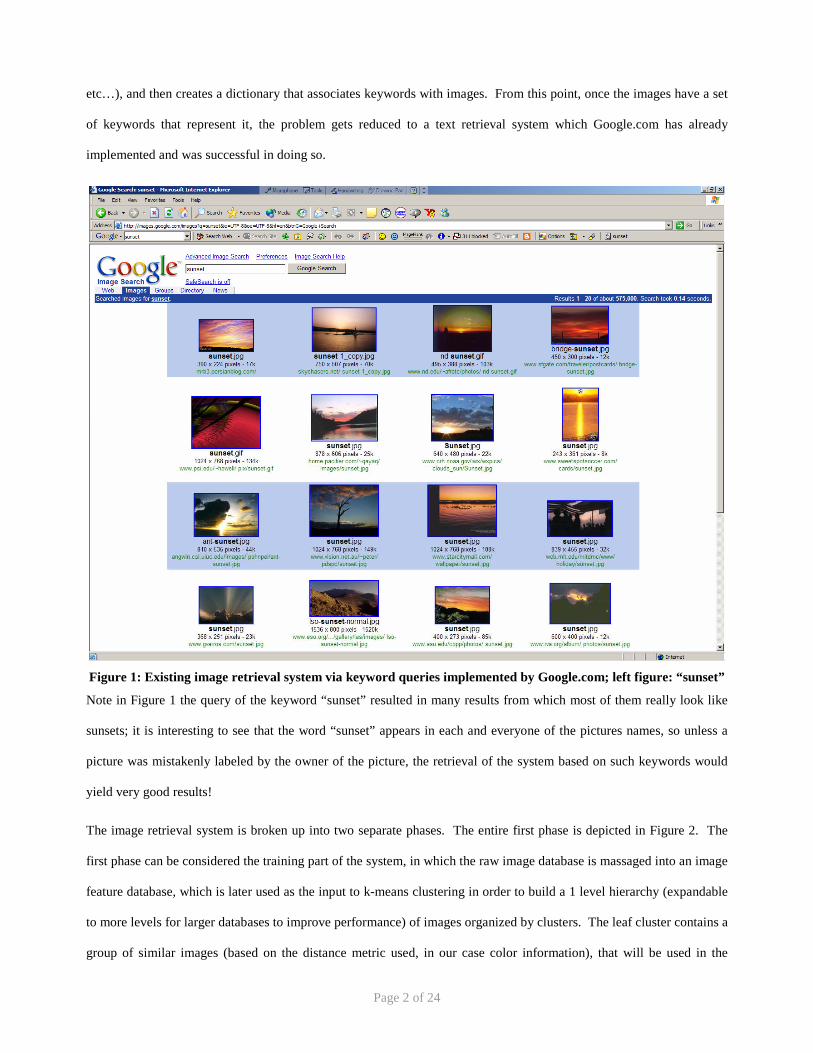
The image retrieval system is broken up into two separate phases. The entire first phase is depicted in Figure 2. The
first phase can be considered the training part of the system, in which the raw image database is massaged into an image
feature database, which is later used as the input to k-means clustering in order to build a 1 level hierarchy (expandable
to more levels for larger databases to improve performance) of images organized by clusters. The leaf cluster contains a
group of similar images (based on the distance metric used, in our case color information), that will be used in the
Page 3 of 24
retrieval phase as the set of images most similar to the query image. The final part of the training phase is visualizing
the image database by displaying the clustroids of the database.
Stage 1
Image Database:Raw Images
Image Database:Image Features
ClusteringClustroid i:
Level 1
Clustroid 1:Level 1
Clustroid sqrt(n):Level 1
Leaf: ImagesLevel 2 Visualization
Stage 2 Stage 3
Figure 2: Image retrieval system overview: training phase
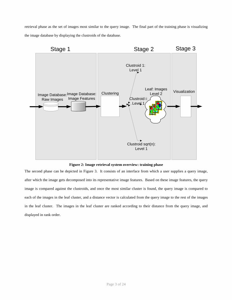
The second phase can be depicted in Figure 3. It consists of an interface from which a user supplies a query image,
after which the image gets decomposed into its representative image features. Based on these image features, the query
image is compared against the clustroids, and once the most similar cluster is found, the query image is compared to
each of the images in the leaf cluster, and a distance vector is calculated from the query image to the rest of the images
in the leaf cluster. The images in the leaf cluster are ranked according to their distance from the query image, and
displayed in rank order.
Page 4 of 24
Stage 1
......
Clustroid i:Level 1
Clustroid 1:Level 1
Clustroid sqrt(n):Level 1
Leaf: ImagesLevel 2
Visualization
Stage 2 Stage 3
Query Image:Raw Image
Query Image:Image Features
Figure 3: Image retrieval system overview: retrieval phase
2.0 RELATED WORK
This section will cover related work regarding image retrieval systems, other implementations, and the state of the art of
today’s image retrieval systems.
The book “Algorithms for Clustering Data” [3] is an excellent source for clustering techniques. There are a few earlier
research efforts on image databases’ exploration. The system described in “Photobook” [4] described a content based
manipulation approach for image databases. The “QBIC” [5] system was developed at IBM and allows queries by
image and video content. The system in “MARS” [6] addresses supporting similarity queries. The system described in
[7] is based on a new data structure built on the multi-linearization of image attributes for efficient organization and fast
visual browsing of the images. The systems proposed in [8]-[9] are based on Hierarchical Self-Organizing Map and are
used to organize a complete image database into a 2-D grid. In [10]-[11] Multi-Dimensional Scaling is used to organize
images returned in response to a query and for direct organization of a complete database. Active browsing is proposed
in [12] by integrating relevance feedback into the browsing environment and thus, users can modify the database
organization to suit a desired task.
Page 5 of 24
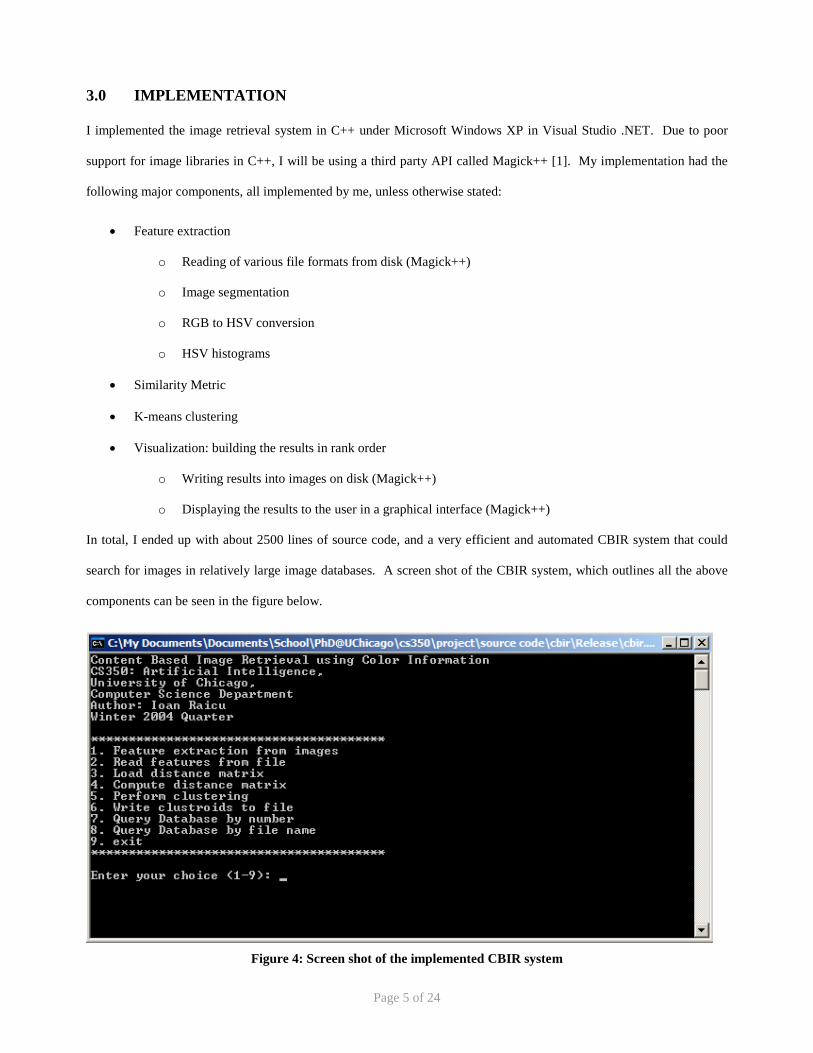
3.0 IMPLEMENTATION
I implemented the image retrieval system in C++ under Microsoft Windows XP in Visual Studio .NET. Due to poor
support for image libraries in C++, I will be using a third party API called Magick++ [1]. My implementation had the
following major components, all implemented by me, unless otherwise stated:
• Feature extraction
o Reading of various file formats from disk (Magick++)
o Image segmentation
o RGB to HSV conversion
o HSV histograms
• Similarity Metric
• K-means clustering
• Visualization: building the results in rank order
o Writing results into images on disk (Magick++)
o Displaying the results to the user in a graphical interface (Magick++)
In total, I ended up with about 2500 lines of source code, and a very efficient and automated CBIR system that could
search for images in relatively large image databases. A screen shot of the CBIR system, which outlines all the above
components can be seen in the figure below.
Figure 4: Screen shot of the implemented CBIR system
Page 6 of 24
3.1 Feature Extraction
We used color as the low-level feature representation in the images of the database. Because the HSV color model is
closely related to the human visual perception, we decided to convert all images from the RGB to the HSV color space.
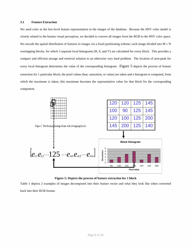
We encode the spatial distribution of features in images via a fixed partitioning scheme; each image divided into M × N
overlapping blocks, for which 3 separate local histograms (H, S, and V) are calculated for every block. This provides a
compact and efficient storage and retrieval solution to an otherwise very hard problem. The location of area-peak for
every local histogram determines the value of the corresponding histogram. Figure 5 depicts the process of feature
extraction for 1 particular block; the pixel values (hue, saturation, or value) are taken and a histogram is computed, from
which the maximum is taken; this maximum becomes the representative value for that block for the corresponding
component.
Block Histogram
012345
90 100 120 125 140 145 200
Pixel value
Occ
uren
ce[ ]eeeee mnmmKKK
211211 125
14012520014520012510012014512590100145125120120
14012520014520012510012014512590100145125120120
Figure 5: Depicts the process of feature extraction for 1 block
Table 1 depicts 2 examples of images decomposed into their feature vector and what they look like when converted
back into their RGB format.

Page 7 of 24
Table 1: Examples of images decomposed into their feature vector and what they look like when converted back into their RGB format
3.1.1 HSV Color Space
It has been verified experimentally that color is perceived through three independent color receptors which have peak
responses at approximately, red, green and blue wavelengths and thus, it can be represented by a linear combination of
the three primary colors (R, G, B) (Figure 6).
Figure 6: Mixture of light (Additive primaries)
Page 8 of 24
The characteristics used to distinguish one color from another are:
• Hue is an attribute associate with the dominant wavelength in a mixture of light waves. It represents the
dominant color as perceived by observer (for example, orange, red, pink, etc)
• Saturation refers to the relative purity or the amount of white light mixed with a hue. Pure colors are fully
saturated. Colors such as pink (red and white) are less saturated with the saturation being inversely
proportioned to the amount of white light added.
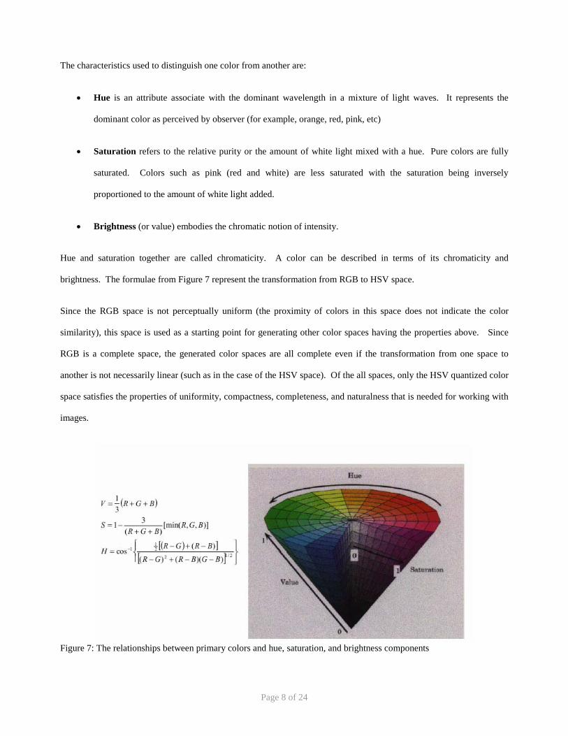
• Brightness (or value) embodies the chromatic notion of intensity.
Hue and saturation together are called chromaticity. A color can be described in terms of its chromaticity and
brightness. The formulae from Figure 7 represent the transformation from RGB to HSV space.
Since the RGB space is not perceptually uniform (the proximity of colors in this space does not indicate the color
similarity), this space is used as a starting point for generating other color spaces having the properties above. Since
RGB is a complete space, the generated color spaces are all complete even if the transformation from one space to
another is not necessarily linear (such as in the case of the HSV space). Of the all spaces, only the HSV quantized color
space satisfies the properties of uniformity, compactness, completeness, and naturalness that is needed for working with
images.
Figure 7: The relationships between primary colors and hue, saturation, and brightness components

Page 9 of 24
3.2 Similarity metric
Clustering methods require that an index of proximity or associations be established between pairs of patterns; a
proximity index is either a similarity or dissimilarity. Since our retrieval system is designed to retrieve the most similar
images with a query image, the proximity index will be defined with respect to similarity. Different similarity measures
have been suggested in the literature to compare images [14, 13].
Let qi and ti represent the block number i in two images Q and T, respectively. Let ( )iii qqq v,s,h and ( )
iii ttt v,s,h
represent the dominant hue-saturation pair of the selected block in the two images Q and T . The block similarity is
defined by the following relationship [15]:
( ) ( ) ( ) ( )iiiiii tqvtqstqh
ii v,vDcs,sD*bh,hDa11t,qS
∗++∗+=
Here hD , sD and vD represent the functions that measure similarity in hue, saturation and value. The constants a ,
b and c define the relative importance of hue, saturation and value in similarity components. Since human perception
is more sensitive to hue, a higher value is assigned to a than to b .
The following function [15] was used to calculate hD :
The function hD explicitly takes into account the fact that hue is measured as an angle. Through empirical evaluations,
when k=2 provides a good non-linearity in the similarity measure to approximate the subjective judgment of the hue
similarity.
The saturation similarity [15] is calculated by:
( )256
sss,sD ii
ii
tqtqs
−=
( ) ⎟⎟⎠
⎞⎜⎜⎝
⎛∗−∗⎟
⎠⎞
⎜⎝⎛−=
2hh
2561cos1h,hD
iiii tqk
tqhπ
Page 10 of 24
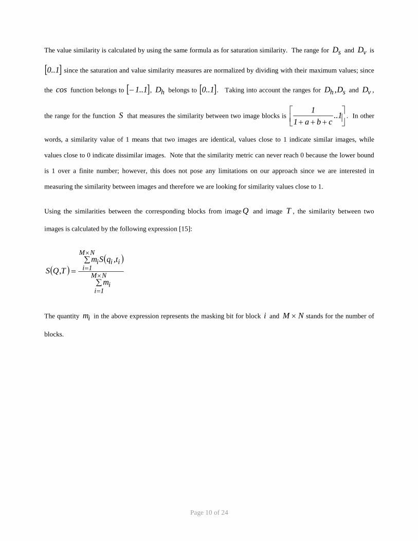
The value similarity is calculated by using the same formula as for saturation similarity. The range for sD and vD is
[ ]1..0 since the saturation and value similarity measures are normalized by dividing with their maximum values; since
the cos function belongs to [ ]1..1− , hD belongs to [ ]1..0 . Taking into account the ranges for sh D,D and vD ,
the range for the function S that measures the similarity between two image blocks is ⎥⎦⎤
⎢⎣⎡
+++1..
cba11
. In other
words, a similarity value of 1 means that two images are identical, values close to 1 indicate similar images, while
values close to 0 indicate dissimilar images. Note that the similarity metric can never reach 0 because the lower bound
is 1 over a finite number; however, this does not pose any limitations on our approach since we are interested in
measuring the similarity between images and therefore we are looking for similarity values close to 1.
Using the similarities between the corresponding blocks from image Q and image T , the similarity between two
images is calculated by the following expression [15]:
( )( )
∑
∑=
×
=
×
=NM
1ii
NM
1iiii
m
t,qSmT,QS
The quantity im in the above expression represents the masking bit for block i and NM × stands for the number of
blocks.

Page 11 of 24
4.0 EMPIRICAL PERFORMANCE RESULTS
I used an image database of 2100 images to test my proof of concept, but a larger database would prove the scalability
of the system empirically. A real nice database that I found is the Corel Stock Photos [2]; it consists of over 39,000
general purpose images; the biggest disadvantage to this image database is that it is prohibitively expensive, and hence I
cannot use it.
4.1 Performance Results
From the performance results given in the next few tables and figures, it can be seen that clustering is a very good
optimization from the performance point of view, and that the implemented system is very scalable. It should be noted
that the entire search time in the entire database is about 3 milliseconds with the 1 level of clustering, while it is about
80 milliseconds with no clustering. The reason it can search so fast through the entire database even without any
clustering is because of the efficient representation of the images by the feature vectors with only 192 components for
each image! The pre-processing stage takes a little over 1 second per image, but when searching through the database,
there is normally only 1 image that is the query, and thus this does not hinder the scalability of the system.
Clusters 1 37 Query Space 1382 74 Feature Space 265344 14208 Time to Cluster (seconds) 0.296838 1.19904 Time to search (seconds) 0.080869 0.003182 Time to extract features in 1 image (seconds) 1.1879 1.09525 Compare images per second 17089.37 23255.81
Table 2: System timing data comparing the clustering approach with no clustering at all
The next table shows the amount of off-line time the system needs to prep itself before queries can be made to the
system. To compute the feature vectors and computing the distance matrix from scratch, it would take about 30 minutes
for about 1400 images, but since this is an off-line process, this is OK. Once these are computed, the data can be loaded
in memory in less than 10 seconds for the entire image database.
Time Reading Features Vectors (seconds) 0.822919Computing Features Vectors (seconds) 1513.636Reading Distance Matrix (seconds) 9.87374Computing Distance Matrix (seconds) 64.12314

Page 12 of 24
Table 3: System Performance timing data for loading/computing the off-line information
The next two figures show how scalable our system is in comparison to a system that would search through the entire
database. For example, www.google.com has about 1,000,000,000 images in their database. Even with this large of a
database, the search (query) space would be less than 100,000 images which can be done on the order of a few seconds.
If we improve the system by having the hierarchy of clusters, we can reduce the search space to only a few hundred
images, and hence retrieve results in a matter of milliseconds!
Query Space
1
10
100
1000
10000
100000
1000000
10000000
100000000
1000000000
1 10 100 1000 10000 100000 1000000 1E+07 1E+08 1E+09
Database Size (Number of Images)
Que
ry S
pace
(Num
ber o
f Im
ages
)
QS - NO C QS - 1 C QS - H sq C QS - H log C
Figure 8: Query Space
In Figure 8 and Figure 9, QS/QT - NO C represents no clustering, QS/QT – 1 C represents 1 level of clustering, QS/QT
– H sq C represents hierarchical clustering with square root of n clusters, where n is the number of images in the level
above, and QS/QT – H log C represents hierarchical clustering with logarithmic number of clusters in relation to the
level above. The notable feature is that even with very large databases (hundreds of millions of images), the CBIR
system could still retrieve the most relevant images in less than a second, which is actually quite amazing when thinking
of the size of the databases we are trying to search.

Page 13 of 24
Query Time
0.00001
0.0001
0.001
0.01
0.1
1
10
100
1000
10000
1 10 100 1000 10000 100000 1000000 10000000 1E+08
Database Size (Number of Images)
Que
ry T
ime
(Sec
onds
)
QT - NO C QT - 1 C QT - H sq C QT - H log C
Figure 9: Query Time
Database Size Mem Req (MB) QS - NO C QS - 1 C QS - H sq C QS - H log C1 0.000732422 0.000732422 0.001465 0.000732 0.000732 10 0.007324219 0.007324219 0.005127 0.005127 0.007324 100 0.073242188 0.073242188 0.014648 0.011719 0.073242 1000 0.732421875 0.732421875 0.046143 0.030762 0.080566
10000 7.32421875 7.32421875 0.146484 0.087891 0.087891 100000 73.2421875 73.2421875 0.462891 0.25708 0.095215 1000000 732.421875 732.421875 1.464844 0.778564 0.102539 10000000 7324.21875 7324.21875 4.631836 2.36792 0.109863 100000000 73242.1875 73242.1875 14.64844 7.324219 0.117188
1000000000 732421.875 732421.875 46.32202 23.31079 0.124512
Table 4: Memory requirements (in megabytes) for the query space
In the above table, we see that all three clustering implementations would have a very small memory requirement,
needing only on the order of dozens of MB which can easily be done even on commodity workstations.
Lastly, we calculated the performance of the system by measuring some statistics regarding the accuracy of the results.
Table 5 depicts these findings. We used 1383 images for the image database, and we used the remaining 718 images to
test the system with. These 718 image were chosen randomly from the entire 2100 images which makes up the
database. For each query, we retrieved the 4 most similar images, and rank them by similarity. The first result indicates

Page 14 of 24
that all retrieved images were color similar to the query image. The second result shows that the semantic meaning
implied by the query image was preserved across 78% of the retrieved images. The third results shows that the most
similar image to the query image retrieved was 91% of the times semantically similar to the query image. The last
result shows that in all query tests done, at least 1 of the 4 images retrieved was semantically similar to the query image.
Description Percentage% all retrieved color similar 100% % all retrieved semantic similar 78% % highest rank semantic similar 91% % at least 1 semantic similar 100%
Table 5: Query retrieval performance results
4.2 Sample Query Results
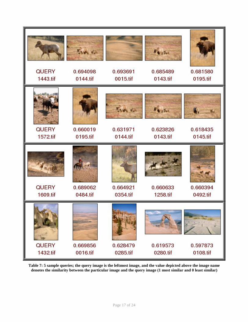
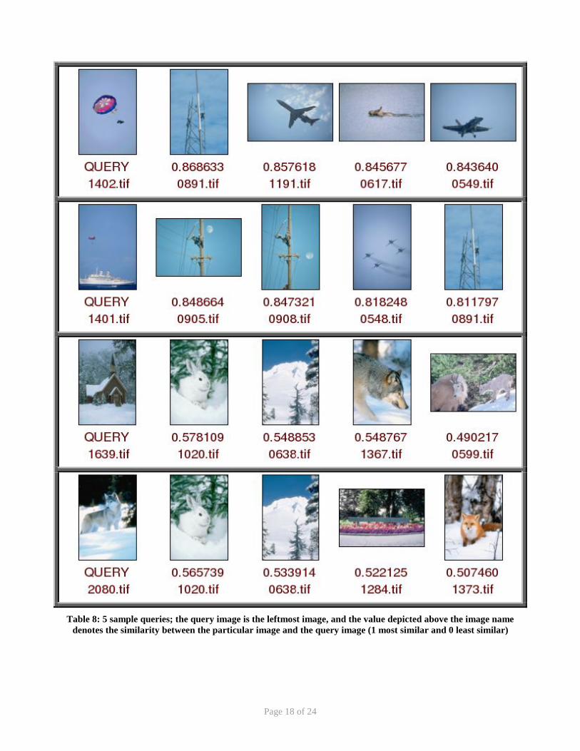
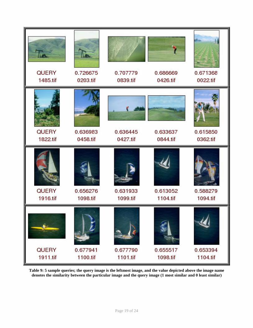
Table 6 through Table 10 show some sample queries performed on the image database. All the rest of the queries
(almost 700 more queries) can be found online at my web site at
http://www.cs.uchicago.edu/~iraicu//research/documents/uchicago/cs350/index.htm.
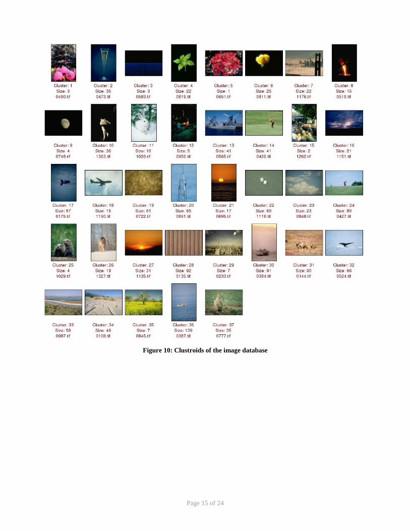
The clustroids of the database can be depicted in Figure 10. Note the varying colors of the clustroids, ranging from
black to various shades of blue, green, orange, red, brown, yellow, and white; it virtually covers the entire color space.
This is the result of a very good similarity metric and the success of the clustering technique used!
The retrieval accuracy is very good, given that the amount of information present in the feature vectors is very small in
comparison to the original images themselves.
Page 15 of 24
Figure 10: Clustroids of the image database

Page 16 of 24
Table 6: 5 sample queries; the query image is the leftmost image, and the value depicted above the image name denotes the similarity between the particular image and the query image (1 most similar and 0 least similar)
Page 17 of 24
Table 7: 5 sample queries; the query image is the leftmost image, and the value depicted above the image name denotes the similarity between the particular image and the query image (1 most similar and 0 least similar)
Page 18 of 24
Table 8: 5 sample queries; the query image is the leftmost image, and the value depicted above the image name denotes the similarity between the particular image and the query image (1 most similar and 0 least similar)
Page 19 of 24
Table 9: 5 sample queries; the query image is the leftmost image, and the value depicted above the image name denotes the similarity between the particular image and the query image (1 most similar and 0 least similar)
Page 20 of 24
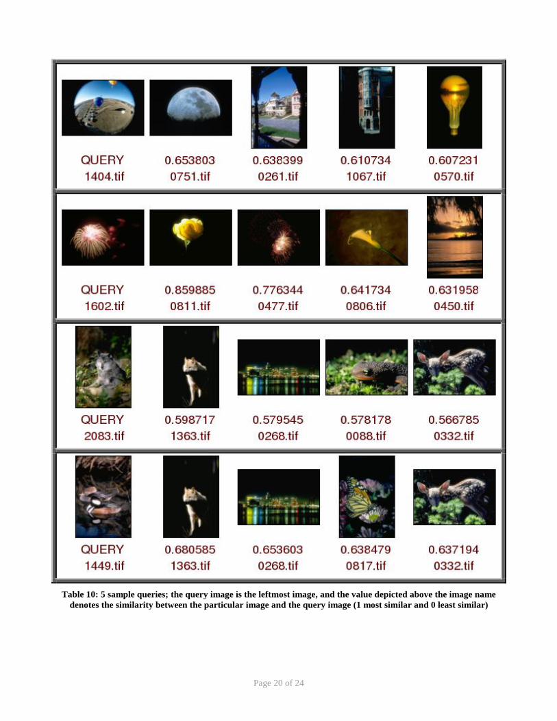
Table 10: 5 sample queries; the query image is the leftmost image, and the value depicted above the image name denotes the similarity between the particular image and the query image (1 most similar and 0 least similar)
Page 21 of 24
5.0 CONCLUSION AND FUTURE WORK
In conclusion, we demonstrated that a CBIR system can be built efficiently that works on real world general images
very well. As the number of digital images increases in our daily lives, the need for some systems will grow and
eventually, these systems will become as common as text search engines have become in the past 10 years! Good CBIR
systems can eventually be used in many domains that currently rely on hand annotating and hand analyzing large
number of images.
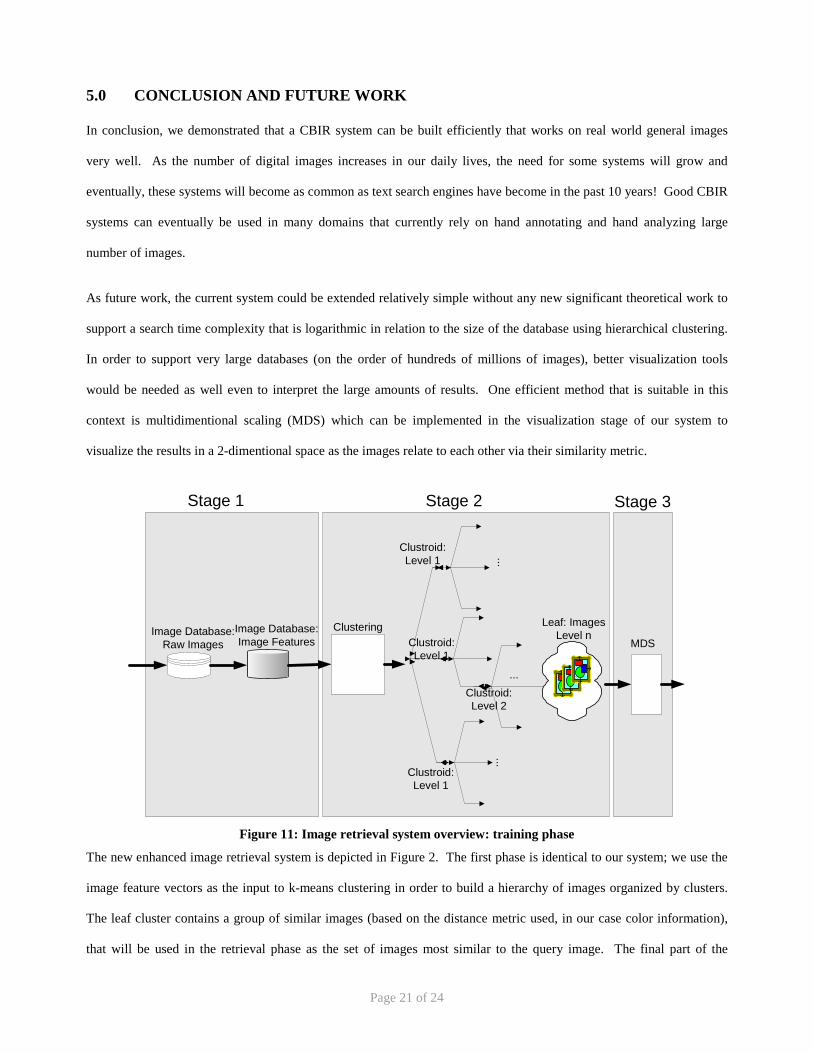
As future work, the current system could be extended relatively simple without any new significant theoretical work to
support a search time complexity that is logarithmic in relation to the size of the database using hierarchical clustering.
In order to support very large databases (on the order of hundreds of millions of images), better visualization tools
would be needed as well even to interpret the large amounts of results. One efficient method that is suitable in this
context is multidimentional scaling (MDS) which can be implemented in the visualization stage of our system to
visualize the results in a 2-dimentional space as the images relate to each other via their similarity metric.
Stage 1
Image Database:Raw Images
Image Database:Image Features
Clustering
......
Clustroid:Level 1
Clustroid:Level 1
Clustroid:Level 1
Clustroid:Level 2
Leaf: ImagesLevel n
...
MDS
Stage 2 Stage 3
Figure 11: Image retrieval system overview: training phase
The new enhanced image retrieval system is depicted in Figure 2. The first phase is identical to our system; we use the
image feature vectors as the input to k-means clustering in order to build a hierarchy of images organized by clusters.
The leaf cluster contains a group of similar images (based on the distance metric used, in our case color information),
that will be used in the retrieval phase as the set of images most similar to the query image. The final part of the
Page 22 of 24
training phase is the multi-dimensional scaling (MDS) technique that will be used to visualize the image database at
varying levels of detail.
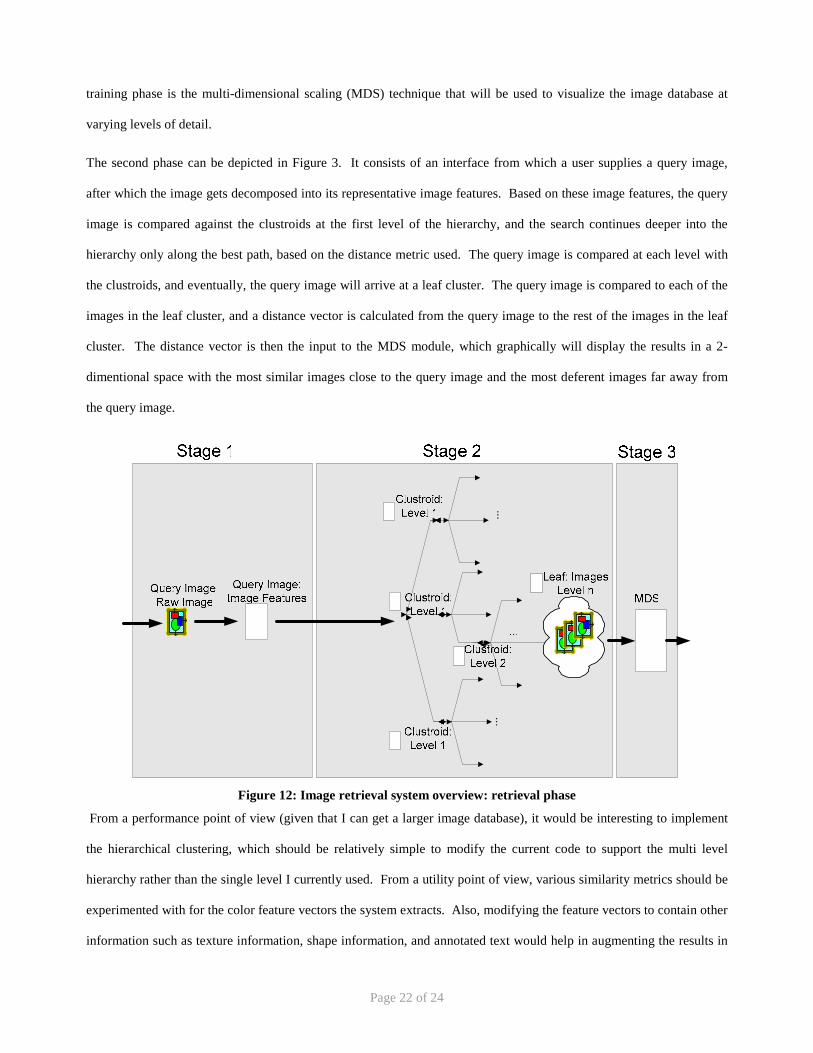
The second phase can be depicted in Figure 3. It consists of an interface from which a user supplies a query image,
after which the image gets decomposed into its representative image features. Based on these image features, the query
image is compared against the clustroids at the first level of the hierarchy, and the search continues deeper into the
hierarchy only along the best path, based on the distance metric used. The query image is compared at each level with
the clustroids, and eventually, the query image will arrive at a leaf cluster. The query image is compared to each of the
images in the leaf cluster, and a distance vector is calculated from the query image to the rest of the images in the leaf
cluster. The distance vector is then the input to the MDS module, which graphically will display the results in a 2-
dimentional space with the most similar images close to the query image and the most deferent images far away from
the query image.
......
Figure 12: Image retrieval system overview: retrieval phase
From a performance point of view (given that I can get a larger image database), it would be interesting to implement
the hierarchical clustering, which should be relatively simple to modify the current code to support the multi level
hierarchy rather than the single level I currently used. From a utility point of view, various similarity metrics should be
experimented with for the color feature vectors the system extracts. Also, modifying the feature vectors to contain other
information such as texture information, shape information, and annotated text would help in augmenting the results in
Page 23 of 24
the system and create a complete end-to-end solution for a CBIR system that would work excellent and efficient at the
same time!
More query results, electronic version of this document, the presentation on this project, and source code can be found
at my web site at http://www.cs.uchicago.edu/~iraicu//research/documents/uchicago/cs350/index.htm. For more
information, comments, or suggestions, I can be reached at [email protected].
6.0 REFERENCES
[1] http://www.simplesystems.org/Magick++/
[2] http://elib.cs.berkeley.edu/photos/corel/
[3] A. K. Jain and R. C. Dubes, Algorithms for Clustering Data, Prentice Hall Advanced Reference Series 1998.
[4] A. Pentland, R. W. Picard, S. Sclaroff, “Photobook: Content Based Manipulation of image databases,” in Multimedia
Tools and Applications, editor Burko Furht, Kluwer Academic Publisher, Boston, pp. 43-80, 1996.
[5] Flickner, M., and et al., Query by Image and Video Content: The QBIC System, IEEE Computer, 1995.
[6] M. Ortega, Y. Rui, K. Chakrabarti, S. Mehrotra, and T. S. Huang, Supporting similarity queries in MARS," ACM
Conf. on Multimedia, 1997.
[7] S. Craver, B.-L. Yeo, and M.M. Yeung. Image browsing using data structure based on multiple space-filling curves.
Proceedings of the Thirty-six Asilomar Conference on Signals, Systems, and Computers, Nov. 1-4, 1998
[8] I.K. Sethi and I. Coman. Image retrieval using hierarchical self-organizing feature maps. Pattern Recognition Letters
20, pp. 1337-1345, 1999
[9] H. Zhang and D. Zhong. A scheme for visual feature based image indexing. Proceedings of SPIE/IS&T Conf. on
Storage and Retrieval for Image and Video Databases III, vol. 2420, pp. 36-46, 1995
[10] J. MacCuish, A. McPherson, J. Barros, and P. Kelly. Interactive layout mechanisms for image database retrieval.
Proceedings of SPIE/IS&T Conf. on Visual Data Exploration and Analysis, III, vol.2656, pp. 104-115, 1996
[11] Y. Rubner, L. Guibas, and C. Tomasi. The earth’s mover distance, multi-dimensional scaling, and color-based image
retrieval. Proceedings of the ARPA Image Understanding Workshop, May 1997
Page 24 of 24
[12] J.-Y. Chen, C.A. Bouman, and J.C. Dalton. Similarity pyramids for browsing and organization of large image
databases. Human Vision and Electronic Imaging III, pp. 563-575, 1998
[13] Faloutsos C. et al. (1993). “Efficient and effective querying by image content”, Technical Report, IBM.
[14] Swain M.J. and Ballard D.H. (1991). “Color Indexing”, International Journal of Computer Vision, 7(1), pp. 11-32.
[15] Sethi I. K., Coman I., Day B. et al. (1998). “Color-WISE: A system for image similarity retrieval using color”,
Proceedings SPIE: Storage and Retrieval for Image and Video Databases, 3132, pp. 140-149.