Searching for the largest bound atoms in space

Downloaded from: https://research.chalmers.se, 2021-11-30 17:51 UTC

Citation for the original published paper (version of record):Emig, K., Salas, P., de Gasperin, F. et al (2020)Searching for the largest bound atoms in spaceAstronomy and Astrophysics, 634http://dx.doi.org/10.1051/0004-6361/201936562

N.B. When citing this work, cite the original published paper.

research.chalmers.se offers the possibility of retrieving research publications produced at Chalmers University of Technology.It covers all kind of research output: articles, dissertations, conference papers, reports etc. since 2004.research.chalmers.se is administrated and maintained by Chalmers Library

(article starts on next page)

A&A 634, A138 (2020)https://doi.org/10.1051/0004-6361/201936562c© ESO 2020

Astronomy&Astrophysics

Searching for the largest bound atoms in spaceK. L. Emig1, P. Salas1,2, F. de Gasperin1,3, J. B. R. Oonk1,4,5, M. C. Toribio1,6, A. P. Mechev1,

H. J. A. Röttgering1, and A. G. G. M. Tielens1

1 Leiden Observatory, Leiden University, PO Box 9513, 2300 RA Leiden, The Netherlandse-mail: emig@strw.leidenuniv.nl

2 Green Bank Observatory, Green Bank, WV 24944, USA3 Hamburger Sternwarte, Universität Hamburg, Gojenbergsweg 112, 21029 Hamburg, Germany4 The Netherlands Institute for Radio Astronomy (ASTRON), PO Box 2, 7990 AA Dwingeloo, The Netherlands5 SURFsara, PO Box 94613, 1090 GP Amsterdam, The Netherlands6 Department of Space, Earth and Environment, Chalmers University of Technology Onsala Space Observatory,

439 92 Onsala, Sweden

Received 23 August 2019 / Accepted 11 October 2019

ABSTRACT

Context. Radio recombination lines (RRLs) at frequencies ν < 250 MHz trace the cold, diffuse phase of the interstellar medium,and yet, RRLs have been largely unexplored outside of our Galaxy. Next-generation low-frequency interferometers such as LOFAR,MWA, and the future SKA will, with unprecedented sensitivity, resolution, and large fractional bandwidths, enable the exploration ofthe extragalactic RRL universe.Aims. We describe methods used to (1) process LOFAR high band antenna (HBA) observations for RRL analysis, and (2) searchspectra for RRLs blindly in redshift space.Methods. We observed the radio quasar 3C 190 (z ≈ 1.2) with the LOFAR HBA. In reducing these data for spectroscopic analysis, weplaced special emphasis on bandpass calibration. We devised cross-correlation techniques that utilize the unique frequency spacingbetween RRLs to significantly identify RRLs in a low-frequency spectrum. We demonstrate the utility of this method by applying itto existing low-frequency spectra of Cassiopeia A and M 82, and to the new observations of 3C 190.Results. Radio recombination lines have been detected in the foreground of 3C 190 at z = 1.12355 (assuming a carbon origin) owingto the first detection of RRLs outside of the local universe (first reported in A&A, 622, A7). Toward the Galactic supernova remnantCassiopeia A, we uncover three new detections: (1) stimulated Cε transitions (∆n = 5) for the first time at low radio frequencies,(2) Hα transitions at 64 MHz with a full width at half-maximum of 3.1 km s−1 the most narrow and one of the lowest frequencydetections of hydrogen to date, and (3) Cα at vLSR ≈ 0 km s−1 in the frequency range 55–78 MHz for the first time. Additionally, werecover Cα, Cβ, Cγ, and Cδ from the −47 km s−1 and −38 km s−1 components. In the nearby starburst galaxy M 82, we do not find asignificant feature. With previously used techniques, we reproduce the previously reported line properties.Conclusions. RRLs have been blindly searched and successfully identified in Galactic (to high-order transitions) and extragalactic (tohigh redshift) observations with our spectral searching method. Our current searches for RRLs in LOFAR observations are limited tonarrow (<100 km s−1) features, owing to the relatively small number of channels available for continuum estimation. Future strategiesmaking use of a wider band (covering multiple LOFAR subbands) or designs with larger contiguous frequency chunks would aidcalibration to deeper sensitivities and broader features.

Key words. galaxies: ISM – radio lines: galaxies – methods: data analysis

1. Introduction

Recombination lines that are observable at low radio frequencies(.1 GHz) involve transitions with principal quantum numbersn & 200. They trace diffuse gas (ne ≈ 0.01−1 cm−3) that can beconsidered cool in temperature (Te ≈ 10−104 K).

Observations in our Galaxy suggest that the most prominentradio recombination lines (RRLs) at ν . 250 MHz arise fromcold (Te ≈ 10−100 K), diffuse (ne ≈ 0.01−0.1 cm−3) gas withindiffuse HI clouds and in clouds surrounding CO-traced molecu-lar gas (Roshi & Kantharia 2011; Salas et al. 2018). This reser-voir of cold gas, referred to as “CO-dark” or “dark-neutral” gas,is missed by CO and HI emission observations. It is estimated tohave a comparable mass to the former two tracers (Grenier et al.2005), however, and is the very site where the formation andde-struction of molecular hydrogen transpires.

In addition, RRLs are compelling tools for studying thephysics of the interstellar medium (ISM) because they can beused to determine physical properties of the gas, specificallythe temperature, density, path length, and radiation field (Shaver1975; Salgado et al. 2017a). Pinning down these properties iskey to describing the physical state of a galaxy and understand-ing the processes of stellar feedback. Radio recombination linemodeling depends not on chemical-dependent or star-formationmodeling, but on (redshift-independent) atomic physics. Becauselow-frequency RRLs are stimulated transitions, they can beobserved to high redshift against bright continuum sources(Shaver 1978). With evidence of stimulated emission being dom-inant in local extragalactic sources at ∼1 GHz (Shaver et al.1978), it is plausible that RRLs can be observed out to z∼ 4.Low-frequency RRLs therefore have a unique potential for prob-ing the ISM in extragalactic sources out to high redshift.

Article published by EDP Sciences A138, page 1 of 19

A&A 634, A138 (2020)

The physical properties of gas can be determined whenRRLs are observed over a range of principal quantum numbers.However, they are extremely faint, with a fractional absorptionof ∼10−3 or lower. At frequencies of ∼150 MHz, RRLs have a∼1 MHz spacing in frequency. By ∼50 MHz, their spacing is∼0.3 MHz. Large fractional bandwidths enable many lines tobe observed simultaneously. On one hand, this helps to con-strain gas properties (e.g., Oonk et al. 2017, hereafter O17). Onthe other, it enables deeper searches through line stacking (e.g.,Balser 2006).

The technical requirements for stimulated RRL observationscan be summarized as follows: (1) large fractional band-widths that span frequency ranges 10−500 MHz for cold, carbongas and 100−800 MHz for (partially) ionized, hydrogen gas;(2) spectral resolutions of ∼0.1 kHz for Galactic observationsand ∼1 kHz for extragalactic; (3) high sensitivity per channel;and (4) spatial resolutions that ideally resolve the .1−100 pcemitting regions. These requirements have inhibited wide-spreadin-depth studies of low-frequency RRLs in the past, largelybecause of the low spatial resolutions and the narrow band-widths of traditional low-frequency instruments, which arisefrom the difficulty of calibrating low-frequency observations thatare affected by the ionosphere.

However, with next-generation low-frequency interferome-ters suchas theLowFrequencyArray(LOFAR;van Haarlem et al.2013), the Murchison Widefield Array (MWA; Tingay et al.2013), and the future Square Kilometer Array (SKA), new pos-sibilities abound for the exploration of the ISM through RRLs.LOFAR has currently been leading the way thanks to its raw sen-sitivity and the flexibility of offering high spectral and spatialresolutions.

LOFAR operates between 10 MHz and 90 MHz via low-bandantennas (LBA) and 110 MHz−250 MHz via high-band antennas(HBA). The array consists of simple inexpensive dipole antennasgrouped into stations. LOFAR is an extremely flexible telescope,offering multiple observing modes (beam-formed, interferomet-ric) and vast ranges of spectral, timing, and spatial resolutions. Itis the first telescope of its kind in the Northern Hemisphere andwill uniquely remain so for the foreseeable future.

The first Galactic RRL analyses with LOFAR have beendirected toward Cassiopeia A (Cas A), a bright supernova rem-nant whose line of sight intersects gas within the Perseus Arm ofthe Galaxy. These studies have highlighted the capability of RRLobservations, and through updated modeling of atomic physics(Salgado et al. 2017b,a), have laid important ground work for thefield in a prototypical source. It was shown that with recombina-tion lines spanning principal quantum numbers of n = 257−584,the electron temperature, density, and path length of cold, diffusegas can be determined to within 15% (O17). Wide bandwidthobservations, especially at the lowest observable frequencies(11 MHz), can be used to constrain the physical properties ofgas together with the α, β, and γ transitions of carbon in a singleobservation (Salas et al. 2017, hereafter S17). Through parsec-resolution and comparisons with other cold-gas tracers, it wasshown that low-frequency RRLs indeed trace CO-dark molec-ular gas on the surfaces of molecular clouds (Salas et al. 2018,hereafter S18). Finally, observations toward Cygnus A demon-strated that bright extragalactic sources can also be used to con-duct Galactic pinhole studies (Oonk et al. 2014).

The first extragalactic observations with LOFAR show thatlow-frequency RRLs provide the means for tracing cold, dif-fuse gas in other galaxies and out to high redshift. These studiesfocused on M 82 (Morabito et al. 2014, hereafter M14), a nearbyprototypical starburst galaxy, and the powerful radio quasar

3C 190 at z ∼ 1.2 (Emig et al. 2019). While these searches areimportant first steps that show RRL detections are possible, theyalso indicate that detailed analyses of stacking are necessary(Emig et al. 2019).

In this article, we cover this much-needed detailed look. Wedescribe the methods behind the detection of RRLs in 3C 190(Emig et al. 2019). We explain processing of LOFAR 110–165 MHz observations for spectroscopic analysis (Sect. 2). Wethen focus on the methods we used to search across redshiftspace for RRLs in a low-frequency spectrum (Sect. 3). We applythis technique to existing 55–78 MHz LOFAR observations ofCas A (Sect. 4) and demonstrate that it can be used to recoverknown RRLs in the spectrum, in addition to previously unknownfeatures. We then focus on the LOFAR observations of M 82 inSect. 5. Section 6 covers the application of our spectral searchto 3C 190. We discuss the utility of the method and implica-tions for future observations in Sect. 7. Conclusions are given inSect. 8.

2. Spectroscopic data reduction

In this section, we cover the implementation of direction-independent spectroscopic calibration for LOFAR HBA(-low)interferometric observations. Special attention is placed on thebandpass because it is one of the most crucial steps and under-lies the main motivations for our strategy.

2.1. HBA bandpass

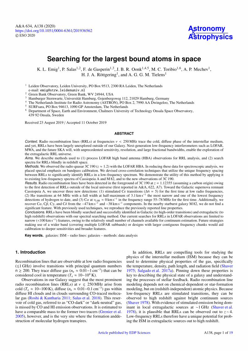
The observed bandpass of LOFAR’s HBA-low (110−190 MHzfilter) is a result of the system response across frequency. It isdependent upon both hardware- and software-related effects. Thephysical structure and orientation of the dual-polarization dipoleantennas influence the global shape of the bandpass. Once thesky signal enters through the antennas, an analog beamformerforms a single station beam. This beam (and the model of it) isfrequency dependent (except at the phase center). The signal istransferred from the station through coaxial cables to a process-ing cabinet. As a result of an impedance mismatch between thecables and receiver units, standing waves are imprinted on thesignal in proportion to the length of the cable. Standing wavescausing the ∼1 MHz ripple are apparent in Fig. 1. An analog fil-ter is then applied; this is responsible for the roll-off at eitherend of the bandpass. Next, after analog-to-digital conversion,a polyphase filter (PPF) is applied to split the data into sub-bands 195.3 kHz wide, which each have fixed central frequen-cies (for a given filter and digital-converter sampling frequency).The data are transported to the off-site correlator through opti-cal fibers. A second PPF is applied, now to each subband, tore-sample the data into channels. This PPF imprints sinusoidalripples within a subband. This can be and is corrected for by theobservatory. However, after the switch to the COBALT correla-tor in 2014, residuals of the PPF are present at the ∼1% level.This PPF is also responsible for in-subband bandpass roll-offthat renders edge channels unusable. In-subband roll-off togetherwith fixed subband central frequencies results in spectralobservations that are processed with non-contiguous frequencycoverage.

Radio frequency interference (RFI) is another major con-tributor to frequency-dependent sensitivity. Of particular hin-drance that has increased over the past years (for comparison, seeOffringa et al. 2013) is digital audio broadcasting (DAB). DABsare broadcast in 1.792 MHz wide channels in the frequency

A138, page 2 of 19

K. L. Emig et al.: Searching for the largest bound atoms in space

120 125 130 135 140 145 150 155 160 165Frequency (MHz)

120

140

160

180

200

Am

plit

ude

Fig. 1. Bandpass solutions of the XX polarization toward the primarycalibrator 3C 196, in which stations are represented with different col-ors. These solutions demonstrate the global shape of the bandpass, aswell a ∼1 MHz ripple that results from a standing wave. Unflagged RFIis still present between 137 and 138 MHz. All core stations have thesame cable length and thus a standing wave of the same periodicity.The fit to the solutions of each station, which is transferred to the target,is shown in black.

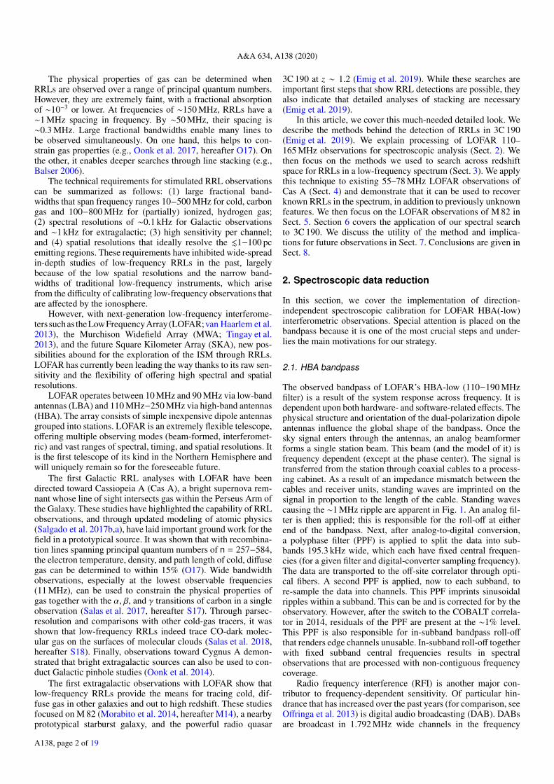
ranges 174−195 MHz. However, with the output power reachingnonlinear proportions (∝P3), intermodulation products of theDABs appear at frequencies of 135, 151, 157, and 162 MHz, aswe show in Fig. 2. The sensitivity and the stability of the band-pass are affected in these regions, rendering data unusable forRRL studies at the most central frequencies.

2.2. Procedure

In this section we describe the reduction of 3C 190 observations.An overview of the steps we take in our data reduction strategyincludes flagging and RFI removal of calibrator data, gain andbandpass solutions toward the primary calibrator, flagging andRFI removal of target data, transfer of bandpass solutions to thetarget, self-calibrated phase and amplitude corrections towardthe target, and imaging. These steps are described in detailbelow.

Processing was performed with the SURFSara Grid pro-cessing facilities1 making use of LOFAR Grid Reduction Tools(Mechev et al. 2017, 2018). It relies on the LOFAR softwareDPPP (van Diepen & Dijkema 2018), LoSoTo (de Gasperin et al.2019), WSCLEAN (Offringa et al. 2014), and AOFlagger(Offringa et al. 2012) to implement the necessary functions.

The observations of 3C 190 were taken with the LOFARHBA-low on 14 January 2017 (Project ID: LC7_027). The setupwas as follows: four hours were spent on 3C 190, with ten min-utes on the primary calibrator 3C 196 before and after. The34 stations of the Dutch array took part in the observations. Fre-quencies between 109.77 MHz and 189.84 MHz were recordedand divided into subbands of 195.3125 kHz. Each subband wasfurther split into 64 channels and recorded at a frequency res-olution of 3.0517 kHz. While taken at 1 s time intervals, RFIremoval and averaging to 2 s were performed by the observatorybefore storing the data.

1 https://www.surf.nl

2.2.1. Preprocessing and flagging

Before calibration, we first implemented a number of flag-ging steps. Using DPPP, we flagged the calibrator measure-ment sets for the remote station baselines, keeping only the24 core stations (CS). Because similar ionospheric conditionsare found above stations this close in proximity (Intema et al.2009; de Gasperin et al. 2018), this heavily reduces direction-dependent effects, and it also avoids the added complicationof solving for the submicrosecond drifting time-stamp of theremote stations (e.g., van Weeren et al. 2016).

As the CS of the HBA are split into two ears, we filtered outthe ear-to-ear cross-correlations. Four channels (at 64-channelresolution) at both edges of each subband are flagged to removebandpass roll-off. With AOFlagger, we used an HBA-specificflagging strategy to further remove RFI. We flagged all datain the frequency ranges 170 MHz–190 MHz due to the DABs(see Sect. 2.1). Additionally, we flagged stations CS006HBA0,CS006HBA1, CS401HBA0, and CS501HBA1 due to bandpassdiscontinuity. The data were then averaged in time and in fre-quency to 6 s and 32 channels per subband (or 6.1034 kHz).

2.2.2. Calibration solutions toward the primary calibrator

With the scan of 3C 196 (ObsID: L565337) taken at the start ofthe observation, we first smoothed the visibilities and weightswith a Gaussian weighting scheme that is proportional with oneover the square of the baseline length (e.g., see de Gasperin et al.2019). With DPPP, we obtained diagonal (XX and YY) gainsolutions toward 3C 196 at full time resolution and with a fre-quency resolution of one subband, while filtering out base-lines shorter than 500 m to avoid large-scale sky emission. Aneight-component sky-model of 3C 196 was used (courtesy of A.Offringa).

Next, we collected the solution tables from each subbandand imported them into LoSoTo. For each channel, we found itsmedian solution across time, the results of which are shown inFig. 1. After 5σ clipping, we fit the amplitude versus frequencysolutions with a rolling window (ten subbands wide) polynomial(sixth order). With a window of ten subbands, we attempted tofit over subband normalization issues, to interpolate over chan-nels that were flagged or contained unflagged RFI, for instance,RFI-contaminated channels between 137 and 138 MHz in Fig. 1,and to avoid transferring per channel scatter to the target. The fitto these solutions is also shown in Fig. 1.

2.2.3. Calibration and imaging of the target field

Flagging and averaging of the target data were performed asdescribed in Sect. 2.2.1. We then applied the bandpass solutionsthat were found with the primary calibrator 3C 196. We nextsmoothed the visibilities with the baseline-dependent smoother.Considering that ionospheric effects were minimal, the CS areall time-stamped by the same clock, and our target 3C 190 is abright and dominant source, we solved explicitly for the diago-nal phases with DPPP with a frequency resolution of one sub-band and at full time resolution while filtering out baselinesshorter than 500 m. We performed this self-calibration using theGlobal Sky Model (van Haarlem et al. 2013), which included128 sources down to 0.1 Jy within a 5◦ radius. We then appliedthese solutions to full-resolution data (32 channels, 6 s).

To correct for beam errors and amplitude scintillation, weperformed a slow amplitude correction. We first averaged the

A138, page 3 of 19

A&A 634, A138 (2020)

110 120 130 140 150 160 170

Frequency (MHz)

100

20

30

40

5060708090

Perc

ent

Fla

gged

Fig. 2. Percentage of flagged visibilities per channel in the calibrated target data. The total percentage here includes ten remote stations and fourcore stations that have been flagged. Broad bumps centered at frequencies of about 135, 151, 157, and 162 MHz show broadband RFI that resultsfrom intermodulation products of DAB amplifiers.

data down to a 30 s time resolution, then smoothed the visibilitieswith the baseline-based weighting scheme. While again filter-ing out baselines shorter than 500 m, we used DPPP to solve theamplitude only every 30 s and twice per subband. Before apply-ing this amplitude correction, we imported the solution tablesfrom each subband into LoSoTo. Using LoSoTo, we clipped out-liers and smoothed the solutions in frequency space with a Gaus-sian with a full width at half-maximum (FWHM) covering foursubbands. These solutions were then applied to full-resolutiondata (32 channels per subband, 6 s).

Our last step was to create an image for each channel.With WSCLEAN, a multi-frequency synthesis image was cre-ated for each subband, from which the clean components wereextracted and used to create channel images of greater depth.Channel images were created with Briggs 0.0 weighting out toan 11× 11 square degrees field of view. We convolved everychannel image to the same resolution of 236′′, which is a fewpercent higher than the lowest resolution image, using CASA(McMullin et al. 2007). The flux density was then extracted froma fixed circular aperture with a diameter of 236′′ using CRRLpy(Salas et al. 2016), and a spectrum was created for each subband.

3. Searching for RRLs in redshift space

The second main focus of this paper covers our method forblindly searching for RRLs across redshift space. Radio recom-bination lines may not be detected individually, but wide-bandwidth observations enable detections as a result of stacking.Because the frequency spacing between each recombination lineis unique (ν ∝ n−2), a unique redshift can be blindly deter-mined with the detection of two or more lines. In stacking acrossredshift space, there are two main issues that require caution.The first is the low N statistics involved in the number of lines(10–30 spectral lines in HBA, 20–50 in LBA) that is used todetermine the stack averaged profile. The second is the relativelysmall number of channels that are available to estimate the con-tinuum in standard (64 channels or fewer per subband) LOFARobservations. The method we employed does not depend on theunique setup of LOFAR and can be applied to observations withother telescopes. The main steps of the method are listed below.1. We assume a redshift and stack the spectra at the location of

available RRLs. This is repeated for a range of redshifts (seeSect. 3.1).

2. We cross-correlate the observed spectrum in optical depthunits with a template spectrum that is populated with Gaussianprofiles at the location of the spectral lines for a given redshift.This is repeated over a range of redshifts (see Sect. 3.2).

3. We cross-correlate the integrated optical depth of the stackedspectrum across redshift with the integrated optical depth ofa template spectrum across redshift in order to corroboratemirror signals (see Sect. 3.3).We compare the values of the normalized cross-correlations,

and identify outliers assuming a normal distribution. Here wenote that a single cross-correlation value is not necessarily mean-ingful in itself, but it is the relative comparison of the cross-correlation values across redshifts which identifies outliers. Werequire both cross-correlations result in a 5σ outlier at each red-shift, as deemed necessary from simulated spectra (Sect. 3.4).When a significant feature is identified by these means, we sub-tract the best fit of the RRL stack. We then repeat the procedureto search for additional transitions or components. In the sectionsbelow, we describe each step in further detail.

3.1. Stacking RRLs

We began processing the spectra by flagging. We manuallyflagged subbands with clearly poor bandpasses. We Doppler cor-rected the observed frequencies because Doppler tracking is notsupported by LOFAR. We flagged additional edge channels thatare affected by bandpass roll-off. Before removing the contin-uum, we flagged and interpolated over channels for which >50%of the visibility data were flagged, as well as channels with a fluxdensity greater than five times the standard deviation.

For a given redshift, we blanked the channels (assuming acertain line width) at the expected frequency of the line whenwe estimated the continuum. For stimulated transitions at lowfrequencies, we have that Iline ≈ Icontτline, where the intensityextracted from the observations is Iobs ≈ Iline + Icont. Therefore,subtracting a continuum fit and dividing by it resulted in the opti-cal depth, (Iobs − Icont)/Icont = τline. The continuum was fit with afirst- or second-order polynomial, chosen based on the χ2 of thefit. Considering the χ2 of the fit and the rms of the subband, weflagged subbands with outlying values.

Taking the central frequency of each subband, we found theRRL closest in frequency and used it to convert frequency unitsinto velocity units. We then linearly interpolated the velocities toa fixed velocity grid, which has a frequency resolution equal to orgreater than the coarsest resolution of all subbands. We weightedsubbands by their rms (w = σ−2). We then stack-averaged allof the N subbands available, where the optical depth of eachchannel is given by

〈τchan〉 =ΣN

i=0(wiτi)

ΣNi=0wi

, (1)

A138, page 4 of 19

K. L. Emig et al.: Searching for the largest bound atoms in space

−0.02 −0.01 0.00 0.01 0.02redshift

−10

−8

−6

−4

−2

0

∫τ

dν

(Hz)

0.0 0.1 0.2 0.3 0.4 0.5 0.6normalized count

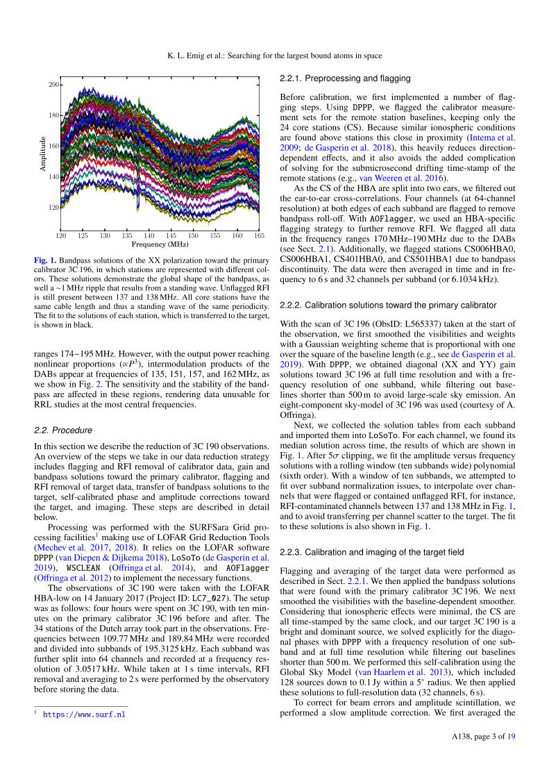
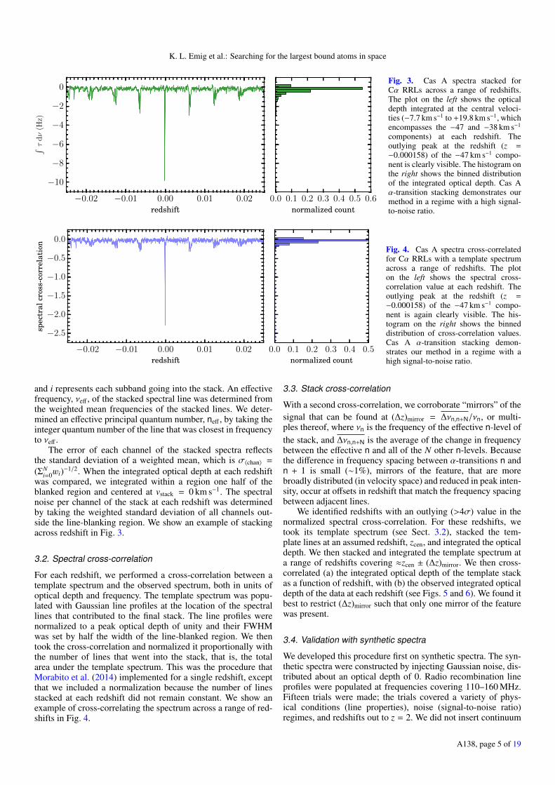
Fig. 3. Cas A spectra stacked forCα RRLs across a range of redshifts.The plot on the left shows the opticaldepth integrated at the central veloci-ties (−7.7 km s−1 to +19.8 km s−1, whichencompasses the −47 and −38 km s−1

components) at each redshift. Theoutlying peak at the redshift (z =−0.000158) of the −47 km s−1 compo-nent is clearly visible. The histogram onthe right shows the binned distributionof the integrated optical depth. Cas Aα-transition stacking demonstrates ourmethod in a regime with a high signal-to-noise ratio.

−0.02 −0.01 0.00 0.01 0.02redshift

−2.5

−2.0

−1.5

−1.0

−0.5

0.0

spec

tral

cros

s-co

rrel

atio

n

0.0 0.1 0.2 0.3 0.4 0.5normalized count

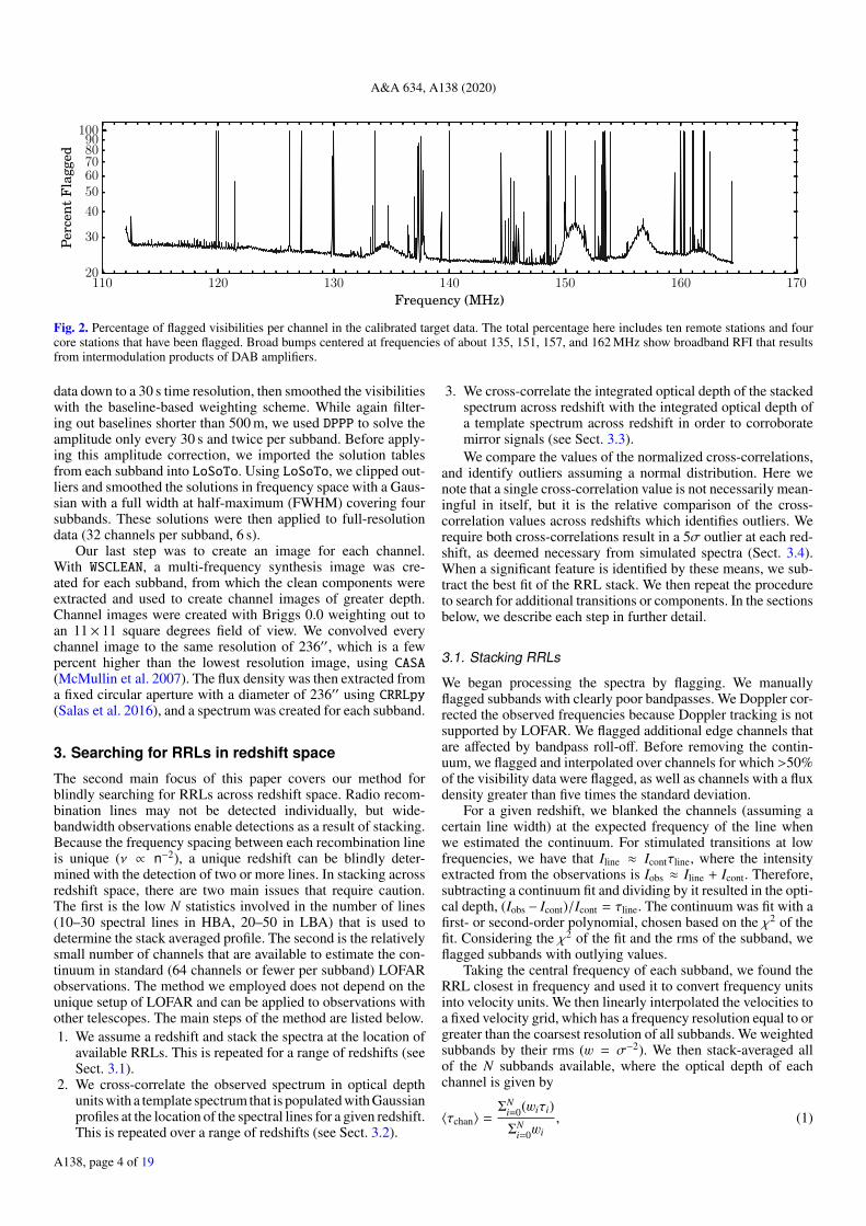
Fig. 4. Cas A spectra cross-correlatedfor Cα RRLs with a template spectrumacross a range of redshifts. The ploton the left shows the spectral cross-correlation value at each redshift. Theoutlying peak at the redshift (z =−0.000158) of the −47 km s−1 compo-nent is again clearly visible. The his-togram on the right shows the binneddistribution of cross-correlation values.Cas A α-transition stacking demon-strates our method in a regime with ahigh signal-to-noise ratio.

and i represents each subband going into the stack. An effectivefrequency, νeff , of the stacked spectral line was determined fromthe weighted mean frequencies of the stacked lines. We deter-mined an effective principal quantum number, neff , by taking theinteger quantum number of the line that was closest in frequencyto νeff .

The error of each channel of the stacked spectra reflectsthe standard deviation of a weighted mean, which is σ〈chan〉 =

(ΣNi=0wi)−1/2. When the integrated optical depth at each redshift

was compared, we integrated within a region one half of theblanked region and centered at vstack = 0 km s−1. The spectralnoise per channel of the stack at each redshift was determinedby taking the weighted standard deviation of all channels out-side the line-blanking region. We show an example of stackingacross redshift in Fig. 3.

3.2. Spectral cross-correlation

For each redshift, we performed a cross-correlation between atemplate spectrum and the observed spectrum, both in units ofoptical depth and frequency. The template spectrum was popu-lated with Gaussian line profiles at the location of the spectrallines that contributed to the final stack. The line profiles werenormalized to a peak optical depth of unity and their FWHMwas set by half the width of the line-blanked region. We thentook the cross-correlation and normalized it proportionally withthe number of lines that went into the stack, that is, the totalarea under the template spectrum. This was the procedure thatMorabito et al. (2014) implemented for a single redshift, exceptthat we included a normalization because the number of linesstacked at each redshift did not remain constant. We show anexample of cross-correlating the spectrum across a range of red-shifts in Fig. 4.

3.3. Stack cross-correlation

With a second cross-correlation, we corroborate “mirrors” of thesignal that can be found at (∆z)mirror = ∆νn,n+N/νn, or multi-ples thereof, where νn is the frequency of the effective n-level ofthe stack, and ∆νn,n+N is the average of the change in frequencybetween the effective n and all of the N other n-levels. Becausethe difference in frequency spacing between α-transitions n andn + 1 is small (∼1%), mirrors of the feature, that are morebroadly distributed (in velocity space) and reduced in peak inten-sity, occur at offsets in redshift that match the frequency spacingbetween adjacent lines.

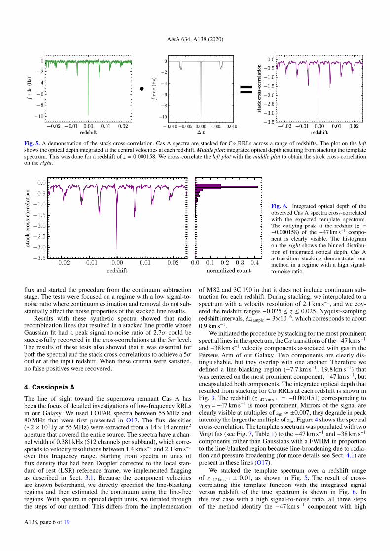
We identified redshifts with an outlying (>4σ) value in thenormalized spectral cross-correlation. For these redshifts, wetook its template spectrum (see Sect. 3.2), stacked the tem-plate lines at an assumed redshift, zcen, and integrated the opticaldepth. We then stacked and integrated the template spectrum ata range of redshifts covering ≈zcen ± (∆z)mirror. We then cross-correlated (a) the integrated optical depth of the template stackas a function of redshift, with (b) the observed integrated opticaldepth of the data at each redshift (see Figs. 5 and 6). We found itbest to restrict (∆z)mirror such that only one mirror of the featurewas present.

3.4. Validation with synthetic spectra

We developed this procedure first on synthetic spectra. The syn-thetic spectra were constructed by injecting Gaussian noise, dis-tributed about an optical depth of 0. Radio recombination lineprofiles were populated at frequencies covering 110–160 MHz.Fifteen trials were made; the trials covered a variety of phys-ical conditions (line properties), noise (signal-to-noise ratio)regimes, and redshifts out to z = 2. We did not insert continuum

A138, page 5 of 19

A&A 634, A138 (2020)

Fig. 5. A demonstration of the stack cross-correlation. Cas A spectra are stacked for Cα RRLs across a range of redshifts. The plot on the leftshows the optical depth integrated at the central velocities at each redshift. Middle plot: integrated optical depth resulting from stacking the templatespectrum. This was done for a redshift of z = 0.000158. We cross-correlate the left plot with the middle plot to obtain the stack cross-correlationon the right.

−0.02 −0.01 0.00 0.01 0.02redshift

−3.5

−3.0

−2.5

−2.0

−1.5

−1.0

−0.5

0.0

stac

kcr

oss-

corr

elat

ion

0.0 0.1 0.2 0.3 0.4normalized count

Fig. 6. Integrated optical depth of theobserved Cas A spectra cross-correlatedwith the expected template spectrum.The outlying peak at the redshift (z =−0.000158) of the −47 km s−1 compo-nent is clearly visible. The histogramon the right shows the binned distribu-tion of integrated optical depth. Cas Aα-transition stacking demonstrates ourmethod in a regime with a high signal-to-noise ratio.

flux and started the procedure from the continuum subtractionstage. The tests were focused on a regime with a low signal-to-noise ratio where continuum estimation and removal do not sub-stantially affect the noise properties of the stacked line results.

Results with these synthetic spectra showed that radiorecombination lines that resulted in a stacked line profile whoseGaussian fit had a peak signal-to-noise ratio of 2.7σ could besuccessfully recovered in the cross-correlations at the 5σ level.The results of these tests also showed that it was essential forboth the spectral and the stack cross-correlations to achieve a 5σoutlier at the input redshift. When these criteria were satisfied,no false positives were recovered.

4. Cassiopeia A

The line of sight toward the supernova remnant Cas A hasbeen the focus of detailed investigations of low-frequency RRLsin our Galaxy. We used LOFAR spectra between 55 MHz and80 MHz that were first presented in O17. The flux densities(∼2 × 104 Jy at 55 MHz) were extracted from a 14× 14 arcmin2

aperture that covered the entire source. The spectra have a chan-nel width of 0.381 kHz (512 channels per subband), which corre-sponds to velocity resolutions between 1.4 km s−1 and 2.1 km s−1

over this frequency range. Starting from spectra in units offlux density that had been Doppler corrected to the local stan-dard of rest (LSR) reference frame, we implemented flaggingas described in Sect. 3.1. Because the component velocitiesare known beforehand, we directly specified the line-blankingregions and then estimated the continuum using the line-freeregions. With spectra in optical depth units, we iterated throughthe steps of our method. This differs from the implementation

of M 82 and 3C 190 in that it does not include continuum sub-traction for each redshift. During stacking, we interpolated to aspectrum with a velocity resolution of 2.1 km s−1, and we cov-ered the redshift ranges −0.025 ≤ z ≤ 0.025, Nyquist-samplingredshift intervals, δzsample = 3×10−6, which corresponds to about0.9 km s−1.

We initiated the procedure by stacking for the most prominentspectral lines in the spectrum, the Cα transitions of the−47 km s−1

and −38 km s−1 velocity components associated with gas in thePerseus Arm of our Galaxy. Two components are clearly dis-tinguishable, but they overlap with one another. Therefore wedefined a line-blanking region (−7.7 km s−1, 19.8 km s−1) thatwas centered on the most prominent component, −47 km s−1, butencapsulated both components. The integrated optical depth thatresulted from stacking for Cα RRLs at each redshift is shown inFig. 3. The redshift (z−47 km s−1 = −0.000151) corresponding tovLSR =−47 km s−1 is most prominent. Mirrors of the signal areclearly visible at multiples of zm ≈ ±0.007; they degrade in peakintensity the larger the multiple of zm. Figure 4 shows the spectralcross-correlation. The template spectrum was populated with twoVoigt fits (see Fig. 7, Table 1) to the −47 km s−1 and −38 km s−1

components rather than Gaussians with a FWHM in proportionto the line-blanked region because line-broadening due to radia-tion and pressure broadening (for more details see Sect. 4.1) arepresent in these lines (O17).

We stacked the template spectrum over a redshift rangeof z−47 km s−1 ± 0.01, as shown in Fig. 5. The result of cross-correlating this template function with the integrated signalversus redshift of the true spectrum is shown in Fig. 6. Inthis test case with a high signal-to-noise ratio, all three stepsof the method identify the −47 km s−1 component with high

A138, page 6 of 19

K. L. Emig et al.: Searching for the largest bound atoms in space

−4

−3

−2

−1

0

Cα(467)34 lines

−1.2−1.0−0.8−0.6−0.4−0.2

0.00.2

Cβ(590)48 lines

−0.5−0.4−0.3−0.2−0.1

0.00.10.2

opti

cal

dep

th(1

0−3)

Cγ(676)54 lines

−0.3

−0.2

−0.1

0.0

0.1

Cδ(743)56 lines

−100 −50 0 50velocityLSR (km s−1)

−0.20−0.15−0.10−0.05

0.000.050.100.15

Cε(801)65 lines

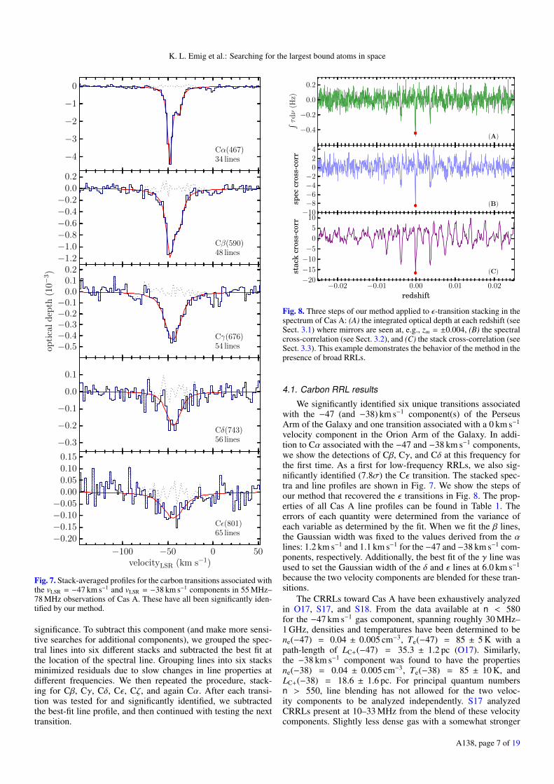
Fig. 7. Stack-averaged profiles for the carbon transitions associated withthe vLSR = −47 km s−1 and vLSR = −38 km s−1 components in 55 MHz–78 MHz observations of Cas A. These have all been significantly iden-tified by our method.

significance. To subtract this component (and make more sensi-tive searches for additional components), we grouped the spec-tral lines into six different stacks and subtracted the best fit atthe location of the spectral line. Grouping lines into six stacksminimized residuals due to slow changes in line properties atdifferent frequencies. We then repeated the procedure, stack-ing for Cβ, Cγ, Cδ, Cε, Cζ, and again Cα. After each transi-tion was tested for and significantly identified, we subtractedthe best-fit line profile, and then continued with testing the nexttransition.

−0.4

−0.2

0.0

0.2

∫τdν

(Hz)

(A)

−10−8−6−4−2

024

spec

cros

s-co

rr

(B)

−0.02 −0.01 0.00 0.01 0.02

redshift

−20

−15

−10

−5

0

5

10

stac

kcr

oss-

corr

(C)

Fig. 8. Three steps of our method applied to ε-transition stacking in thespectrum of Cas A: (A) the integrated optical depth at each redshift (seeSect. 3.1) where mirrors are seen at, e.g., zm = ±0.004, (B) the spectralcross-correlation (see Sect. 3.2), and (C) the stack cross-correlation (seeSect. 3.3). This example demonstrates the behavior of the method in thepresence of broad RRLs.

4.1. Carbon RRL results

We significantly identified six unique transitions associatedwith the −47 (and −38) km s−1 component(s) of the PerseusArm of the Galaxy and one transition associated with a 0 km s−1

velocity component in the Orion Arm of the Galaxy. In addi-tion to Cα associated with the −47 and −38 km s−1 components,we show the detections of Cβ, Cγ, and Cδ at this frequency forthe first time. As a first for low-frequency RRLs, we also sig-nificantly identified (7.8σ) the Cε transition. The stacked spec-tra and line profiles are shown in Fig. 7. We show the steps ofour method that recovered the ε transitions in Fig. 8. The prop-erties of all Cas A line profiles can be found in Table 1. Theerrors of each quantity were determined from the variance ofeach variable as determined by the fit. When we fit the β lines,the Gaussian width was fixed to the values derived from the αlines: 1.2 km s−1 and 1.1 km s−1 for the −47 and −38 km s−1 com-ponents, respectively. Additionally, the best fit of the γ line wasused to set the Gaussian width of the δ and ε lines at 6.0 km s−1

because the two velocity components are blended for these tran-sitions.

The CRRLs toward Cas A have been exhaustively analyzedin O17, S17, and S18. From the data available at n < 580for the −47 km s−1 gas component, spanning roughly 30 MHz–1 GHz, densities and temperatures have been determined to bene(−47) = 0.04 ± 0.005 cm−3, Te(−47) = 85 ± 5 K with apath-length of LC+(−47) = 35.3 ± 1.2 pc (O17). Similarly,the −38 km s−1 component was found to have the propertiesne(−38) = 0.04 ± 0.005 cm−3, Te(−38) = 85 ± 10 K, andLC+(−38) = 18.6 ± 1.6 pc. For principal quantum numbersn > 550, line blending has not allowed for the two veloc-ity components to be analyzed independently. S17 analyzedCRRLs present at 10–33 MHz from the blend of these velocitycomponents. Slightly less dense gas with a somewhat stronger

A138, page 7 of 19

A&A 634, A138 (2020)

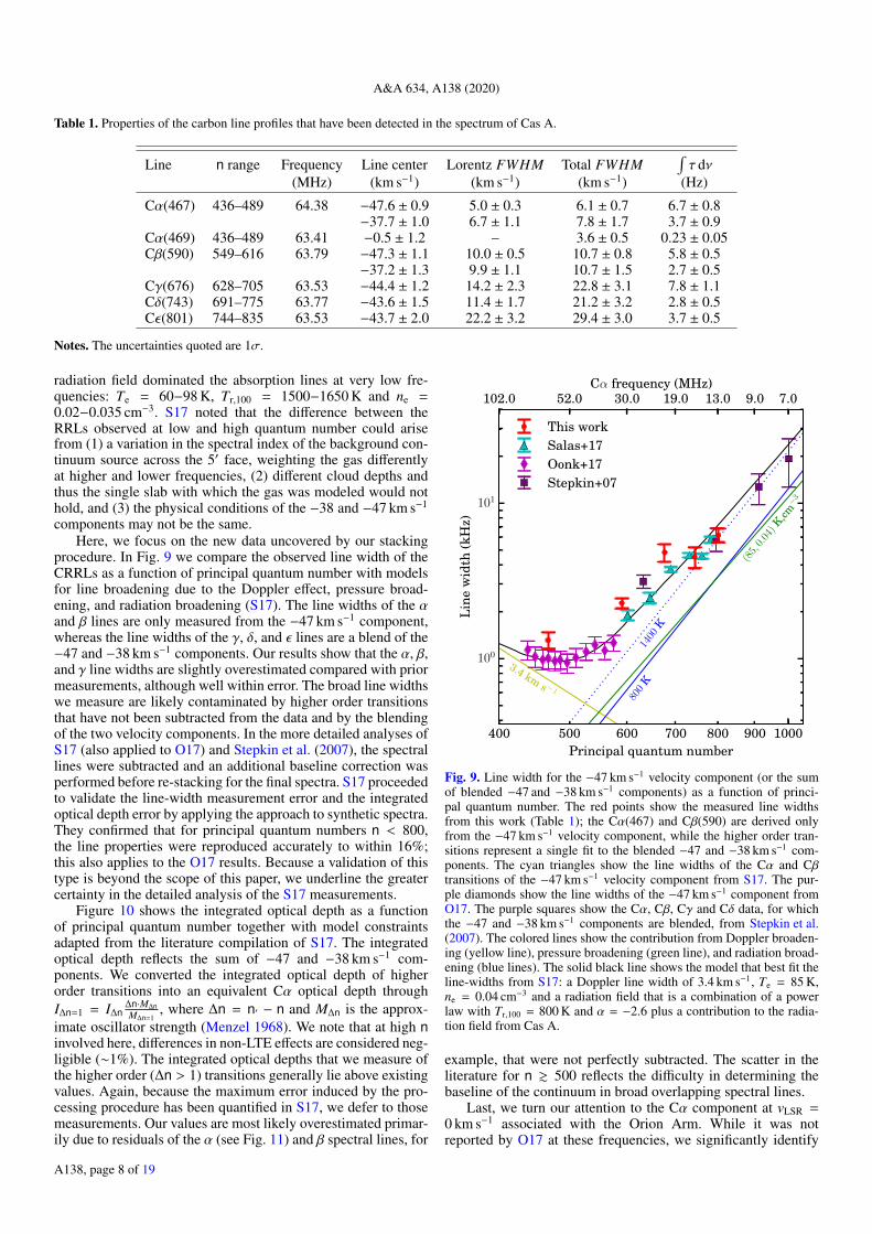
Table 1. Properties of the carbon line profiles that have been detected in the spectrum of Cas A.

Line n range Frequency Line center Lorentz FWHM Total FWHM∫τ dν

(MHz) (km s−1) (km s−1) (km s−1) (Hz)

Cα(467) 436–489 64.38 −47.6 ± 0.9 5.0 ± 0.3 6.1 ± 0.7 6.7 ± 0.8−37.7 ± 1.0 6.7 ± 1.1 7.8 ± 1.7 3.7 ± 0.9

Cα(469) 436–489 63.41 −0.5 ± 1.2 – 3.6 ± 0.5 0.23 ± 0.05Cβ(590) 549–616 63.79 −47.3 ± 1.1 10.0 ± 0.5 10.7 ± 0.8 5.8 ± 0.5

−37.2 ± 1.3 9.9 ± 1.1 10.7 ± 1.5 2.7 ± 0.5Cγ(676) 628–705 63.53 −44.4 ± 1.2 14.2 ± 2.3 22.8 ± 3.1 7.8 ± 1.1Cδ(743) 691–775 63.77 −43.6 ± 1.5 11.4 ± 1.7 21.2 ± 3.2 2.8 ± 0.5Cε(801) 744–835 63.53 −43.7 ± 2.0 22.2 ± 3.2 29.4 ± 3.0 3.7 ± 0.5

Notes. The uncertainties quoted are 1σ.

radiation field dominated the absorption lines at very low fre-quencies: Te = 60−98 K, Tr,100 = 1500−1650 K and ne =0.02−0.035 cm−3. S17 noted that the difference between theRRLs observed at low and high quantum number could arisefrom (1) a variation in the spectral index of the background con-tinuum source across the 5′ face, weighting the gas differentlyat higher and lower frequencies, (2) different cloud depths andthus the single slab with which the gas was modeled would nothold, and (3) the physical conditions of the −38 and −47 km s−1

components may not be the same.Here, we focus on the new data uncovered by our stacking

procedure. In Fig. 9 we compare the observed line width of theCRRLs as a function of principal quantum number with modelsfor line broadening due to the Doppler effect, pressure broad-ening, and radiation broadening (S17). The line widths of the αand β lines are only measured from the −47 km s−1 component,whereas the line widths of the γ, δ, and ε lines are a blend of the−47 and −38 km s−1 components. Our results show that the α, β,and γ line widths are slightly overestimated compared with priormeasurements, although well within error. The broad line widthswe measure are likely contaminated by higher order transitionsthat have not been subtracted from the data and by the blendingof the two velocity components. In the more detailed analyses ofS17 (also applied to O17) and Stepkin et al. (2007), the spectrallines were subtracted and an additional baseline correction wasperformed before re-stacking for the final spectra. S17 proceededto validate the line-width measurement error and the integratedoptical depth error by applying the approach to synthetic spectra.They confirmed that for principal quantum numbers n < 800,the line properties were reproduced accurately to within 16%;this also applies to the O17 results. Because a validation of thistype is beyond the scope of this paper, we underline the greatercertainty in the detailed analysis of the S17 measurements.

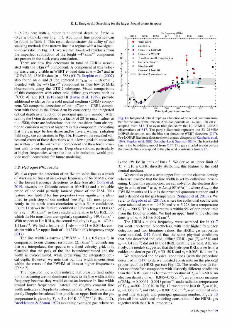
Figure 10 shows the integrated optical depth as a functionof principal quantum number together with model constraintsadapted from the literature compilation of S17. The integratedoptical depth reflects the sum of −47 and −38 km s−1 com-ponents. We converted the integrated optical depth of higherorder transitions into an equivalent Cα optical depth throughI∆n=1 = I∆n

∆n·M∆nM∆n=1

, where ∆n = n′ − n and M∆n is the approx-imate oscillator strength (Menzel 1968). We note that at high ninvolved here, differences in non-LTE effects are considered neg-ligible (∼1%). The integrated optical depths that we measure ofthe higher order (∆n > 1) transitions generally lie above existingvalues. Again, because the maximum error induced by the pro-cessing procedure has been quantified in S17, we defer to thosemeasurements. Our values are most likely overestimated primar-ily due to residuals of the α (see Fig. 11) and β spectral lines, for

1000400 500 600 700 800 900Principal quantum number

100

101

Lin

ew

idth

(kH

z)

3.4 km s −1

1400

K

800

K

(85,

0.04

)K,cm

−3

This workSalas+17Oonk+17Stepkin+07

102.0 52.0 30.0 19.0 13.0 9.0 7.0Cα frequency (MHz)

Fig. 9. Line width for the −47 km s−1 velocity component (or the sumof blended −47 and −38 km s−1 components) as a function of princi-pal quantum number. The red points show the measured line widthsfrom this work (Table 1); the Cα(467) and Cβ(590) are derived onlyfrom the −47 km s−1 velocity component, while the higher order tran-sitions represent a single fit to the blended −47 and −38 km s−1 com-ponents. The cyan triangles show the line widths of the Cα and Cβtransitions of the −47 km s−1 velocity component from S17. The pur-ple diamonds show the line widths of the −47 km s−1 component fromO17. The purple squares show the Cα, Cβ, Cγ and Cδ data, for whichthe −47 and −38 km s−1 components are blended, from Stepkin et al.(2007). The colored lines show the contribution from Doppler broaden-ing (yellow line), pressure broadening (green line), and radiation broad-ening (blue lines). The solid black line shows the model that best fit theline-widths from S17: a Doppler line width of 3.4 km s−1, Te = 85 K,ne = 0.04 cm−3 and a radiation field that is a combination of a powerlaw with Tr,100 = 800 K and α = −2.6 plus a contribution to the radia-tion field from Cas A.

example, that were not perfectly subtracted. The scatter in theliterature for n & 500 reflects the difficulty in determining thebaseline of the continuum in broad overlapping spectral lines.

Last, we turn our attention to the Cα component at vLSR =0 km s−1 associated with the Orion Arm. While it was notreported by O17 at these frequencies, we significantly identify

A138, page 8 of 19

K. L. Emig et al.: Searching for the largest bound atoms in space

it (5.2σ) here with a rather faint optical depth of∫τdν =

(0.23 ± 0.05) Hz (see Fig. 11). Additional line properties canbe found in Table 1. This result demonstrates the utility of ourstacking methods for a narrow line in a regime with a low signal-to-noise ratio. In Fig. 11C we see that low-level residuals fromthe imperfect subtraction of the bright −47 km s−1 componentare present in the stack cross-correlation.

There are now five detections in total of CRRLs associ-ated with the 0 km s−1 component. A component at this veloc-ity was clearly visible in WSRT P-band data at n = 267 and inLOFAR 33–45 MHz data (n ∼ 588) (O17). Stepkin et al. (2007)also found an α and β line centered at vLSR = −1.6 km s−1,blended with the −47 km s−1 component in their low 26 MHzobservations using the UTR-2 telescope. Visual comparisonsof this component with other cold diffuse gas tracers, such as13CO(1-0) and [CI] (S18) and HI (Payne et al. 1989), provideadditional evidence for a cold neutral medium (CNM) compo-nent. We compared detections of the −47 km s−1 CRRL compo-nent with those in the Orion Arm by considering the integratedoptical depth as a function of principal quantum number. Afterscaling the Orion detections by a factor of 20 (to match values atn ∼ 500), there are indications that the transition from absorp-tion to emission occurs at higher n in this component, indicatingthat the gas may be less dense and/or have a warmer radiationfield (e.g., see constraints in Fig. 10). However, the rescaled val-ues and errors of these detections with a low signal-to-noise raioare within 3σ of the −47 km s−1 component and therefore consis-tent with its derived properties. Deep observations, particularlyat higher frequencies where the line is in emission, would pro-vide useful constraints for future modeling.

4.2. Hydrogen RRL results

We also report the detection of an Hα emission line as a resultof stacking 43 lines at an average frequency of 64.08 MHz, oneof the lowest frequency detections to date (see also Oonk et al.2019, towards the Galactic center at 63 MHz) and a valuableprobe of the cold partially ionized phase of the ISM. Thisfeature (see Table 2 for line properties) was significantly iden-tified in each step of our method (see Fig. 11), most promi-nently in the stack cross-correlation with a 5.4σ confidence.Figure 11 shows the feature identified at a redshift z = 0.000337or vLSR = 101 km s−1 as these stacks are relative to Cα RRL, forwhich the Hα transitions are regularly separated by 149.4 km s−1.With respect to Hα RRLs, the central velocity is vLSR = −47.9±1.1 km s−1. We find a feature of

∫τdν = −0.21 ± 0.04 Hz, con-

sistent with a 3σ upper limit of −0.42 Hz in this frequency range(O17).

The line width is narrow (FWHM = 3.1 ± 0.5 km s−1) incomparison to our channel resolution (2.1 km s−1); consideringthat we interpolated the spectra to a fixed velocity grid, it isplausible that the peak of the line is underestimated and thewidth is overestimated, while preserving the integrated opti-cal depth. However, we note that our line width is consistentwithin the errors of the FWHM of lines at higher frequencies(Table 2).

The measured line widths indicate that pressure (and radia-tion) broadening are not dominant effects to the line width at thisfrequency because they would cause an increase in line widthtoward lower frequencies. Instead, the roughly constant linewidth indicates a Doppler-broadened profile. When we assume apurely Doppler-broadened line-profile, an upper limit on the gastemperature is given by Te < 2 × 104 K ( 30.25 km s−1

∆v )2 (Eq. (4.7),Brocklehurst & Seaton 1972) assuming hydrogen gas, where ∆v

200 300 400 500 600 700 800 900−20

0

20

40

60

80

100

This workSalas+17Oonk+17 LOFAROonk+17 WSRTKantharia+98 compilationSorochenko+10Stepkin+07Oonk+17 best fitSalas+17 constraints

816.0 242.0 102.0 52.0 30.0 19.0 13.0 9.0Cα frequency (MHz)

Inte

grat

edop

tica

ldep

th(H

z)

Principal quantum number

Fig. 10. Integrated optical depth as a function of principal quantum num-ber for the sum of the Perseus Arm components at −47 and −38 km s−1

adapted from S17. The cyan triangles show the 10–33 MHz LOFARobservations of S17. The purple diamonds represent the 33–78 MHzLOFAR detections, and the blue star shows the WSRT detection (O17).Pre-LOFAR literature data are shown as gray data points (Kantharia et al.1998; Stepkin et al. 2007; Sorochenko & Smirnov 2010). The black solidline is the best-fitting model from O17. The gray shaded region coversthe models that correspond to the physical constraints from S17.

is the FWHM in units of km s−1. We derive an upper limit ofTe < 210 ± 0.5 K, directly attributing this feature to the coldneutral medium.

We can also place a strict upper limit on the electron densitywhen we assume that the line width is set by collisional broad-ening. Under this assumption, we can solve for the electron den-sity in units of cm−3 as ne = ∆νcol(10anγ/π)−1, where ∆νcol is theFWHM in units of Hz, n is the principal quantum number, and aand γ depend on the gas temperature (Salgado et al. 2017a). Werefer to Salgado et al. (2017a), where the collisional coefficientswere tabulated as a = −9.620 and γ = 5.228 for a temperatureof Te = 200 K. This temperature is within 5% of our upper limitfrom the Doppler profile. We find an upper limit to the electrondensity of ne < 0.10 ± 0.02 cm−3.

The HRRLs at this frequency were searched for in O17but went undetected. Nonetheless, with their higher frequencydetection and two literature values, the HRRL gas propertieswere modeled. O17 found that the same physical conditionsthat best described the cold, diffuse CRRL gas (Te = 85 K andne = 0.04 cm−3) did not fit the HRRL emitting gas best. Alterna-tively, the models suggested that the hydrogen RRLs arise from acolder and denser gas (Te = 30−50 K and ne = 0.065−0.11 cm−3).

We remodeled the physical conditions (with the proceduredescribed in O17) to derive updated constraints on the physicalproperties of the HRRL gas (see Fig. 12). The results provide fur-ther evidence for a component with distinctly different conditionsthan the CRRL gas: an electron temperature of Te = 30−50 K, anelectron density of ne = 0.045−0.75 cm−3, an emission measureof EMH+ = 0.00064−0.0018 pc cm−6, and a radiation temperatureof Tr,100 = 800−2000 K. In Fig. 12, we plot the best fit, Te = 40 K,ne = 0.06 cm−3, and EMH+ = 0.0012 pc cm−6, as a function of inte-grated line strength and principal quantum number. Figure 13plots all line-width and modeling constraints of the HRRL gastogether with the CRRL properties.

A138, page 9 of 19

A&A 634, A138 (2020)

−0.15

−0.10

−0.05

0.00

0.05

0.10

0.15

∫τ

dν

(Hz)

(A)

−3

−2

−1

0

1

2

3

spec

cros

s-co

rr

(B)

−0.02 −0.01 0.00 0.01 0.02redshift

−2

−1

0

1

2

3

stac

kcr

oss-

corr

(C)

−100 −50 0

velocityLSR (km s−1)

−0.2

−0.1

0.0

0.1

0.2

0.3

opti

cal

dep

th(1

0−3) Hα(468)

43 lines

−50 0 50

velocityLSR (km s−1)

−0.4

−0.3

−0.2

−0.1

0.0

0.1

opti

cal

dep

th(1

0−3)

Cα(469)

36 lines

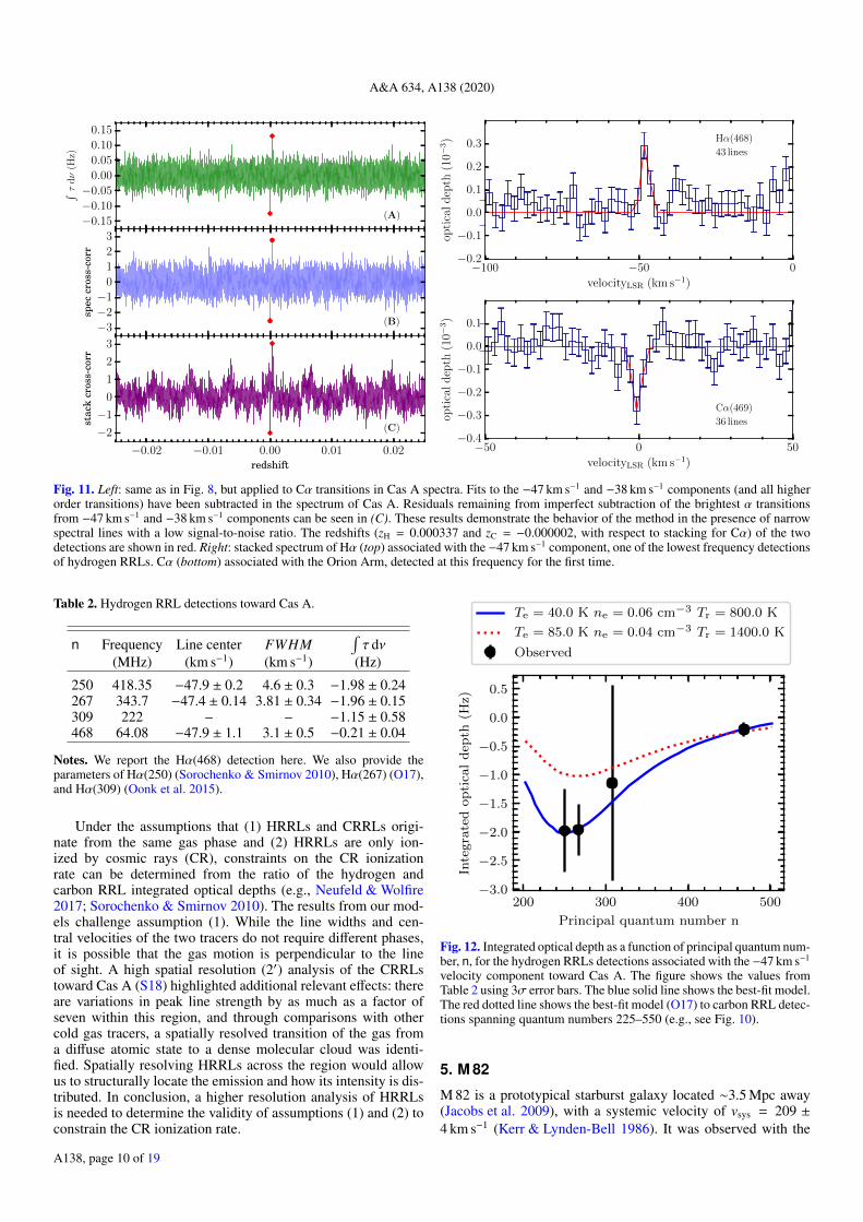
Fig. 11. Left: same as in Fig. 8, but applied to Cα transitions in Cas A spectra. Fits to the −47 km s−1 and −38 km s−1 components (and all higherorder transitions) have been subtracted in the spectrum of Cas A. Residuals remaining from imperfect subtraction of the brightest α transitionsfrom −47 km s−1 and −38 km s−1 components can be seen in (C). These results demonstrate the behavior of the method in the presence of narrowspectral lines with a low signal-to-noise ratio. The redshifts (zH = 0.000337 and zC = −0.000002, with respect to stacking for Cα) of the twodetections are shown in red. Right: stacked spectrum of Hα (top) associated with the −47 km s−1 component, one of the lowest frequency detectionsof hydrogen RRLs. Cα (bottom) associated with the Orion Arm, detected at this frequency for the first time.

Table 2. Hydrogen RRL detections toward Cas A.

n Frequency Line center FWHM∫τ dν

(MHz) (km s−1) (km s−1) (Hz)

250 418.35 −47.9 ± 0.2 4.6 ± 0.3 −1.98 ± 0.24267 343.7 −47.4 ± 0.14 3.81 ± 0.34 −1.96 ± 0.15309 222 – – −1.15 ± 0.58468 64.08 −47.9 ± 1.1 3.1 ± 0.5 −0.21 ± 0.04

Notes. We report the Hα(468) detection here. We also provide theparameters of Hα(250) (Sorochenko & Smirnov 2010), Hα(267) (O17),and Hα(309) (Oonk et al. 2015).

Under the assumptions that (1) HRRLs and CRRLs origi-nate from the same gas phase and (2) HRRLs are only ion-ized by cosmic rays (CR), constraints on the CR ionizationrate can be determined from the ratio of the hydrogen andcarbon RRL integrated optical depths (e.g., Neufeld & Wolfire2017; Sorochenko & Smirnov 2010). The results from our mod-els challenge assumption (1). While the line widths and cen-tral velocities of the two tracers do not require different phases,it is possible that the gas motion is perpendicular to the lineof sight. A high spatial resolution (2′) analysis of the CRRLstoward Cas A (S18) highlighted additional relevant effects: thereare variations in peak line strength by as much as a factor ofseven within this region, and through comparisons with othercold gas tracers, a spatially resolved transition of the gas froma diffuse atomic state to a dense molecular cloud was identi-fied. Spatially resolving HRRLs across the region would allowus to structurally locate the emission and how its intensity is dis-tributed. In conclusion, a higher resolution analysis of HRRLsis needed to determine the validity of assumptions (1) and (2) toconstrain the CR ionization rate.

200 300 400 500

Principal quantum number n

−3.0

−2.5

−2.0

−1.5

−1.0

−0.5

0.0

0.5

Inte

gra

ted

opti

cal

dep

th(H

z)

Te = 40.0 K ne = 0.06 cm−3 Tr = 800.0 K

Te = 85.0 K ne = 0.04 cm−3 Tr = 1400.0 K

Observed

Fig. 12. Integrated optical depth as a function of principal quantum num-ber, n, for the hydrogen RRLs detections associated with the −47 km s−1

velocity component toward Cas A. The figure shows the values fromTable 2 using 3σ error bars. The blue solid line shows the best-fit model.The red dotted line shows the best-fit model (O17) to carbon RRL detec-tions spanning quantum numbers 225–550 (e.g., see Fig. 10).

5. M 82

M 82 is a prototypical starburst galaxy located ∼3.5 Mpc away(Jacobs et al. 2009), with a systemic velocity of vsys = 209 ±4 km s−1 (Kerr & Lynden-Bell 1986). It was observed with the

A138, page 10 of 19

K. L. Emig et al.: Searching for the largest bound atoms in space

102

Electron temperature (K)

100

101

Ele

ctro

npr

essu

re(K

cm−

3)

ne= 0.1

cm−3

linewidthHRRLCRRL

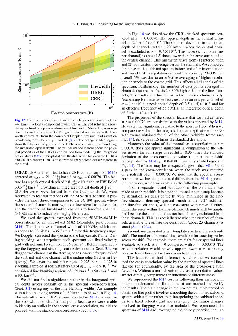
Fig. 13. Electron pressure as a function of electron temperature of the−47 km s−1 velocity component toward Cas A. The red solid line showsthe upper limit of a pressure-broadened line width. Shaded regions rep-resent 1σ and 3σ uncertainty. The green shaded regions show the line-width constraints from the combined Doppler, pressure, and radiationbroadening terms for Tr,100 = 1400 K (S17). The orange shaded regionsshow the physical properties of the HRRLs constrained from modelingthe integrated optical depth. The yellow shaded regions show the phys-ical properties of the CRRLs constrained from modeling the integratedoptical depth (O17). This plot shows the distinction between the HRRLsand CRRLs, where HRRLs arise from slightly colder, denser regions inthe cloud.

LOFAR LBA and reported to have CRRLs in absorption (M14)centered at vLSR = 211.3+0.7

−0.5 km s−1 or zcen = 0.00070. The fea-ture has a peak optical depth of 2.8+0.12

−0.10 ×10−3 and an FWHM of30.6+2.3

−1.0 km s−1, providing an integrated optical depth of∫τdν =

21.3 Hz; errors were derived from the Gaussian fit. We weremotivated to test our methods on the M 82 data because it pro-vides the most direct comparison to the 3C 190 spectra, wherethe spectral feature is narrow, has a low signal-to-noise ratio,and the fraction of line-blanked channels to line-free channels(&10%) starts to induce non-negligible effects.

We used the spectra extracted from the 50 MHz–64 MHzobservations of an unresolved M 82 (Morabito, priv. comm.;M14). The data have a channel width of 6.10 kHz, which cor-responds to 28.6 km s−1–36.7 km s−1 over this frequency range.We Doppler corrected the spectra to the barycentric frame. Dur-ing stacking, we interpolated each spectrum to a fixed velocitygrid with a channel resolution of 36.7 km s−1. Before implement-ing the flagging and stacking routine described in Sect. 3.1, weflagged two channels at the starting edge (lower in frequency) ofthe subband and one channel at the ending edge (higher in fre-quency). We cover the redshift ranges −0.025 ≤ z ≤ 0.025 instacking, sampled at redshift intervals of δzsample = 6× 10−5. Weconsidered line-blanking regions of ±25 km s−1, ±50 km s−1, and±100 km s−1.

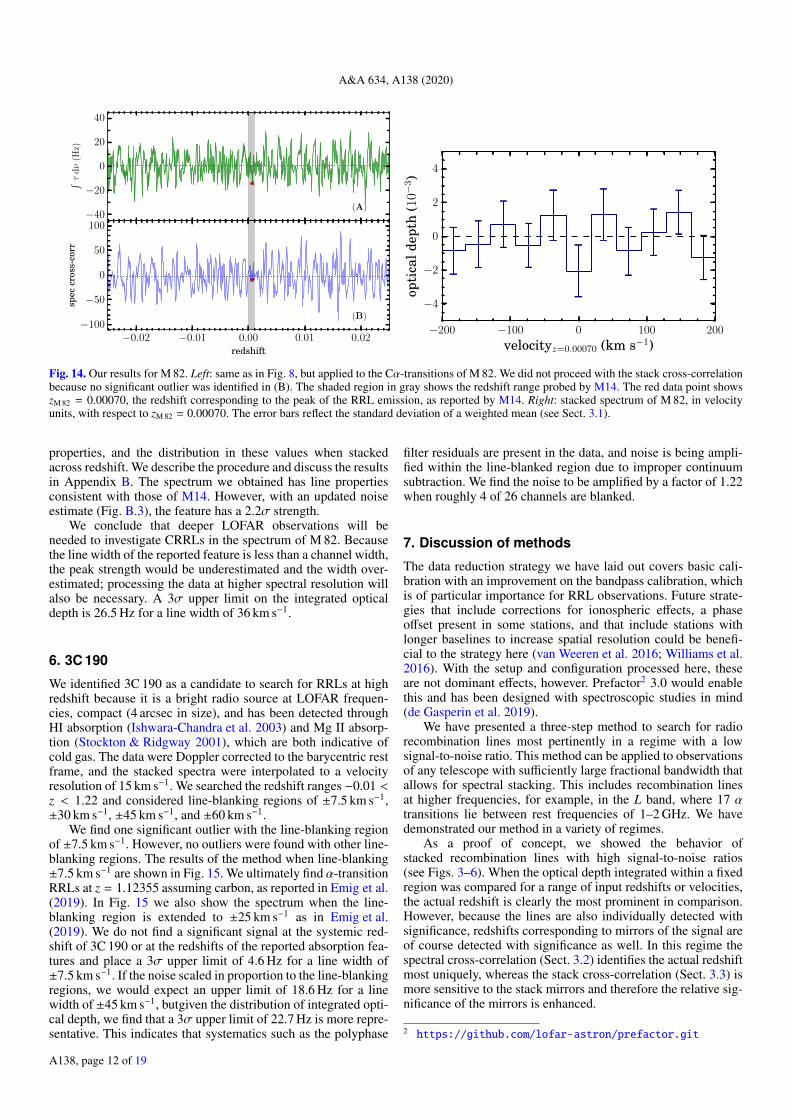
We did not find a significant outlier in the integrated opti-cal depth across redshift or in the spectral cross-correlation(Sect. 3.2) using any of the line-blanking widths. An examplewith a line-blanking region of ±50 km s−1 is shown in Fig. 14.The redshift at which RRLs were reported in M14 is shown inthe plots with a red circular data point. Because we were unableto identify an outlier in the spectral cross-correlation, we did notproceed with the stack cross-correlation (Sect. 3.3).

In Fig. 14 we also show the CRRL stacked spectrum cen-tered at z = 0.00070. The optical depth in the central chan-nel is (2.1 ± 1.5) × 10−3. The standard deviation in the opticaldepth of channels within ±200 km s−1 when the central chan-nel is excluded is σ = 9.7 × 10−4. This noise (which is an rmsper channel) is about 1.5 times lower than the error attributed tothe central channel. This mismatch arises from (1) interpolationand (2) non-uniform coverage across the channels. We comparedthe noise in the subband spectra before and after interpolation,and found that interpolation reduced the noise by 20–30%; anoverall 6% was due to an effective averaging of higher resolu-tion channels to the coarse grid. This affects all channels of thespectrum. Furthermore, the number of data points averaged inchannels that are line free is 20–30% higher than in the line chan-nels; this results in a lower rms in the line-free channels only.Accounting for these two effects results in an rms per channel ofσ = 1.4×10−3, a peak optical depth of (2.5±1.4)×10−3, and foran effective frequency of 55.5 MHz, an integrated optical depthof∫τdν = 18 ± 10 Hz.

The properties of the spectral feature that we find centeredat z = 0.00070 are consistent with the values reported by M14.However, the significance relative to the noise is 1.8σ. When wecompare the value of the integrated optical depth at z = 0.00070with values obtained for all of the other redshifts tested (seeFig. 14), its value is 1.5 times the standard deviation.

Moreover, the value of the spectral cross-correlation at z =0.00070 does not appear significant in comparison to the val-ues across the full range of redshifts (0.35 times the standarddeviation of the cross-correlation values), nor in the redshiftrange probed by M14 (z = 0.0–0.001; see gray shaded region inFig. 14). The latter may be unexpected, given that M14 founda peak in the cross-correlation when the stack was centeredon a redshift of z = 0.00073. We note that the spectral cross-correlation we have implemented differs from the M14 approachin three ways, which we explain in the following paragraphs.

First, a separate fit and subtraction of the continuum wasmade at each redshift. It is essential to include this step becauseby definition, residuals of the fit were minimized in the line-free channels; thus any spectral search in the “off” redshifts,the line-free channels, will be consistent with noise. Further-more, the error within the line-blanked channels will be ampli-fied because the continuum has not been directly estimated fromthese channels. This is especially true when the number of chan-nels available to estimate the continuum (about 25 channels) issmall (Sault 1994).

Second, we generated a new template spectrum for each red-shift. The number of spectral lines available for stacking variesacross redshift. For example, there are eight fewer spectral linesavailable to stack at z = 0 compared with z = 0.00070. Thecross-correlation would naively appear lower at z = 0 onlybecause fewer lines fall within a searchable region.

This leads to the third difference, which is that we normal-ized the cross-correlation value by the number of spectral linesstacked (or equivalently, by the area of the cross-correlationfunction). Without a normalization, the cross-correlation valuesare not directly comparable for functions of different areas.

We reproduced the M14 results following their methods, inorder to understand the limitations of our method and verifythe results. The main change in the procedures implemented toobtain the line profile involves smoothing the combined subbandspectra with a filter rather than interpolating the subband spec-tra to a fixed velocity grid and averaging. The minor changesinvolved in flagging were also included. We reproduced thespectrum of M14 and investigated the noise properties, the line

A138, page 11 of 19

A&A 634, A138 (2020)

−40

−20

0

20

40

∫τ

dν

(Hz)

(A)

−0.02 −0.01 0.00 0.01 0.02redshift

−100

−50

0

50

100

spec

cros

s-co

rr

(B)

−200 −100 0 100 200

velocityz=0.00070 (km s−1)

−4

−2

0

2

4

opti

cald

epth

(10−

3)

Fig. 14. Our results for M 82. Left: same as in Fig. 8, but applied to the Cα-transitions of M 82. We did not proceed with the stack cross-correlationbecause no significant outlier was identified in (B). The shaded region in gray shows the redshift range probed by M14. The red data point showszM 82 = 0.00070, the redshift corresponding to the peak of the RRL emission, as reported by M14. Right: stacked spectrum of M 82, in velocityunits, with respect to zM 82 = 0.00070. The error bars reflect the standard deviation of a weighted mean (see Sect. 3.1).

properties, and the distribution in these values when stackedacross redshift. We describe the procedure and discuss the resultsin Appendix B. The spectrum we obtained has line propertiesconsistent with those of M14. However, with an updated noiseestimate (Fig. B.3), the feature has a 2.2σ strength.

We conclude that deeper LOFAR observations will beneeded to investigate CRRLs in the spectrum of M 82. Becausethe line width of the reported feature is less than a channel width,the peak strength would be underestimated and the width over-estimated; processing the data at higher spectral resolution willalso be necessary. A 3σ upper limit on the integrated opticaldepth is 26.5 Hz for a line width of 36 km s−1.

6. 3C 190

We identified 3C 190 as a candidate to search for RRLs at highredshift because it is a bright radio source at LOFAR frequen-cies, compact (4 arcsec in size), and has been detected throughHI absorption (Ishwara-Chandra et al. 2003) and Mg II absorp-tion (Stockton & Ridgway 2001), which are both indicative ofcold gas. The data were Doppler corrected to the barycentric restframe, and the stacked spectra were interpolated to a velocityresolution of 15 km s−1. We searched the redshift ranges −0.01 <z < 1.22 and considered line-blanking regions of ±7.5 km s−1,±30 km s−1, ±45 km s−1, and ±60 km s−1.

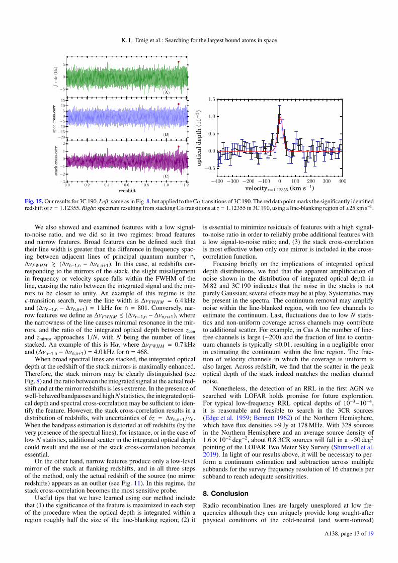
We find one significant outlier with the line-blanking regionof ±7.5 km s−1. However, no outliers were found with other line-blanking regions. The results of the method when line-blanking±7.5 km s−1 are shown in Fig. 15. We ultimately find α-transitionRRLs at z = 1.12355 assuming carbon, as reported in Emig et al.(2019). In Fig. 15 we also show the spectrum when the line-blanking region is extended to ±25 km s−1 as in Emig et al.(2019). We do not find a significant signal at the systemic red-shift of 3C 190 or at the redshifts of the reported absorption fea-tures and place a 3σ upper limit of 4.6 Hz for a line width of±7.5 km s−1. If the noise scaled in proportion to the line-blankingregions, we would expect an upper limit of 18.6 Hz for a linewidth of ±45 km s−1, butgiven the distribution of integrated opti-cal depth, we find that a 3σ upper limit of 22.7 Hz is more repre-sentative. This indicates that systematics such as the polyphase

filter residuals are present in the data, and noise is being ampli-fied within the line-blanked region due to improper continuumsubtraction. We find the noise to be amplified by a factor of 1.22when roughly 4 of 26 channels are blanked.

7. Discussion of methods

The data reduction strategy we have laid out covers basic cali-bration with an improvement on the bandpass calibration, whichis of particular importance for RRL observations. Future strate-gies that include corrections for ionospheric effects, a phaseoffset present in some stations, and that include stations withlonger baselines to increase spatial resolution could be benefi-cial to the strategy here (van Weeren et al. 2016; Williams et al.2016). With the setup and configuration processed here, theseare not dominant effects, however. Prefactor2 3.0 would enablethis and has been designed with spectroscopic studies in mind(de Gasperin et al. 2019).

We have presented a three-step method to search for radiorecombination lines most pertinently in a regime with a lowsignal-to-noise ratio. This method can be applied to observationsof any telescope with sufficiently large fractional bandwidth thatallows for spectral stacking. This includes recombination linesat higher frequencies, for example, in the L band, where 17 αtransitions lie between rest frequencies of 1–2 GHz. We havedemonstrated our method in a variety of regimes.

As a proof of concept, we showed the behavior ofstacked recombination lines with high signal-to-noise ratios(see Figs. 3–6). When the optical depth integrated within a fixedregion was compared for a range of input redshifts or velocities,the actual redshift is clearly the most prominent in comparison.However, because the lines are also individually detected withsignificance, redshifts corresponding to mirrors of the signal areof course detected with significance as well. In this regime thespectral cross-correlation (Sect. 3.2) identifies the actual redshiftmost uniquely, whereas the stack cross-correlation (Sect. 3.3) ismore sensitive to the stack mirrors and therefore the relative sig-nificance of the mirrors is enhanced.

2 https://github.com/lofar-astron/prefactor.git

A138, page 12 of 19

K. L. Emig et al.: Searching for the largest bound atoms in space

−5

0

5

∫τ

dν

(Hz)

(A)

−20

−15

−10

−5

0

5

10

15

spec

cros

s-co

rr

(B)

0.0 0.2 0.4 0.6 0.8 1.0 1.2

redshift

−3

−2

−1

0

1

2

stac

kcr

oss-

corr

(C)

−400 −300 −200 −100 0 100 200 300 400

velocityz=1.12355 (km s−1)

−0.5

0.0

0.5

1.0

1.5

opti

cald

epth

(10−

3)

Fig. 15. Our results for 3C 190. Left: same as in Fig. 8, but applied to the Cα transitions of 3C 190. The red data point marks the significantly identifiedredshift of z = 1.12355. Right: spectrum resulting from stacking Cα transitions at z = 1.12355 in 3C 190, using a line-blanking region of±25 km s−1.

We also showed and examined features with a low signal-to-noise ratio, and we did so in two regimes: broad featuresand narrow features. Broad features can be defined such thattheir line width is greater than the difference in frequency spac-ing between adjacent lines of principal quantum number n,∆νFWHM & (∆νn−1,n − ∆νn,n+1). In this case, at redshifts cor-responding to the mirrors of the stack, the slight misalignmentin frequency or velocity space falls within the FWHM of theline, causing the ratio between the integrated signal and the mir-rors to be closer to unity. An example of this regime is theε-transition search, were the line width is ∆νFWHM = 6.4 kHzand (∆νn−1,n − ∆νn,n+1) = 1 kHz for n = 801. Conversely, nar-row features we define as ∆νFWHM . (∆νn−1,n − ∆νn,n+1), wherethe narrowness of the line causes minimal resonance in the mir-rors, and the ratio of the integrated optical depth between zcenand zmirror approaches 1/N, with N being the number of linesstacked. An example of this is Hα, where ∆νFWHM = 0.7 kHzand (∆νn−1,n − ∆νn,n+1) = 4.0 kHz for n = 468.

When broad spectral lines are stacked, the integrated opticaldepth at the redshift of the stack mirrors is maximally enhanced.Therefore, the stack mirrors may be clearly distinguished (seeFig. 8) and the ratio between the integrated signal at the actual red-shift and at the mirror redshifts is less extreme. In the presence ofwell-behavedbandpassesandhigh N statistics, the integratedopti-cal depth and spectral cross-correlation may be sufficient to iden-tify the feature. However, the stack cross-correlation results in adistribution of redshifts, with uncertainties of δz = ∆νn,n+1/νn.When the bandpass estimation is distorted at off redshifts (by thevery presence of the spectral lines), for instance, or in the case oflow N statistics, additional scatter in the integrated optical depthcould result and the use of the stack cross-correlation becomesessential.

On the other hand, narrow features produce only a low-levelmirror of the stack at flanking redshifts, and in all three stepsof the method, only the actual redshift of the source (no mirrorredshifts) appears as an outlier (see Fig. 11). In this regime, thestack cross-correlation becomes the most sensitive probe.

Useful tips that we have learned using our method includethat (1) the significance of the feature is maximized in each stepof the procedure when the optical depth is integrated within aregion roughly half the size of the line-blanking region; (2) it

is essential to minimize residuals of features with a high signal-to-noise ratio in order to reliably probe additional features witha low signal-to-noise ratio; and, (3) the stack cross-correlationis most effective when only one mirror is included in the cross-correlation function.

Focusing briefly on the implications of integrated opticaldepth distributions, we find that the apparent amplification ofnoise shown in the distribution of integrated optical depth inM 82 and 3C 190 indicates that the noise in the stacks is notpurely Gaussian; several effects may be at play. Systematics maybe present in the spectra. The continuum removal may amplifynoise within the line-blanked region, with too few channels toestimate the continuum. Last, fluctuations due to low N statis-tics and non-uniform coverage across channels may contributeto additional scatter. For example, in Cas A the number of line-free channels is large (∼200) and the fraction of line to contin-uum channels is typically ≤0.01, resulting in a negligible errorin estimating the continuum within the line region. The frac-tion of velocity channels in which the coverage is uniform isalso larger. Across redshift, we find that the scatter in the peakoptical depth of the stack indeed matches the median channelnoise.

Nonetheless, the detection of an RRL in the first AGN wesearched with LOFAR holds promise for future exploration.For typical low-frequency RRL optical depths of 10−3−10−4,it is reasonable and feasible to search in the 3CR sources(Edge et al. 1959; Bennett 1962) of the Northern Hemisphere,which have flux densities >9 Jy at 178 MHz. With 328 sourcesin the Northern Hemisphere and an average source density of1.6 × 10−2 deg−2, about 0.8 3CR sources will fall in a ∼50 deg2

pointing of the LOFAR Two Meter Sky Survey (Shimwell et al.2019). In light of our results above, it will be necessary to per-form a continuum estimation and subtraction across multiplesubbands for the survey frequency resolution of 16 channels persubband to reach adequate sensitivities.

8. Conclusion

Radio recombination lines are largely unexplored at low fre-quencies although they can uniquely provide long sought-afterphysical conditions of the cold-neutral (and warm-ionized)

A138, page 13 of 19

A&A 634, A138 (2020)

phase(s) of the ISM. We have described methods for calibrat-ing and extracting RRLs in low-frequency (<170 MHz) spectra.Starting with LOFAR observations that are optimized for extra-galactic sources (where line widths may be 10–100 km s−1 andcan plausibly be probed to z ∼ 4), we discussed spectroscopicdata reduction. We then showed a procedure in which spectraare stacked and cross-correlated to identify features with a lowsignal-to-noise ratio. One cross-correlation was taken betweena template spectrum and the observed spectrum, both in opticaldepth units, where the location of each line was used. A secondcross-correlation incorporated the average spacing between lines(and their line width); the integrated optical depth over a rangeof redshifts was cross-correlated with the distribution of the tem-plate spectrum over a range of redshifts, corroborating what werefer to as “mirrors” of the stack at flanking redshifts.

Our method was developed to blindly search in redshift forRRLs in the LOFAR HBA spectrum of 3C 190, in which wehave identified an RRL in emission at z = 1.12355 ± 0.00005(assuming a carbon origin). This was the first detection of RRLsoutside of the local Universe (Emig et al. 2019). To demonstrateand test the limitations of the method, we also applied it to exist-ing LOFAR observations of the sources Cas A and M 82.

We reanalyzed the 55–78 MHz LOFAR spectra of Cas A.Usingourmethods,wediscovered threenewdetections in thedata,plus the original detections of Oonk et al. (2017). We significantlydetect Cα(n = 467), Cβ(590), Cγ(676), Cδ(743), and Cε(801)transitions associated with the line-of-sight −47 km s−1 and/or−38 km s−1 components.This is thefirstdetectionofanε transition(∆n = 5) at low radio frequencies. We also find Hα(468) in emis-sion at 64.08 MHz with

∫τdν= (−0.21 ± 0.04) Hz and a FWHM

of 3.1 km s−1, resulting in one of the lowest frequency and mostnarrow detections of hydrogen. The line width directly associatesthis hydrogen with the cold, ionized component of the ISM; thisis further supported by our updated modeling of the gas physicalproperties with best-fit conditions of Te = 40 K, ne = 0.06 cm−3,and EMH+ = 0.0012 pc cm−6. Additionally, we detect Cα associ-ated with the Orion Arm at 0 km s−1 at these frequencies for thefirst time.

For the 55–64 MHz spectra of the nearby starburst galaxyM 82, we recovered the line properties reported by Morabito et al.(2014) and found that the integrated optical depth is ∼2σ relativeto the noise. A 3σ upper limit on the integrated optical depth is26.5 Hz. Follow-up LOFAR observations reaching deeper sensi-tivities and higher spectral resolution will be worthwhile.

We find that LOFAR observations using 32 channels per sub-band are not optimal for RRL studies. Because few channelsare available to estimate the continuum, the noise in the line-blanking region is amplified. Currently, continuum subtractioncan only be estimated within a single subband. As the non-overlapping nature of the narrow (195.3 kHz) subbands makesa smooth bandpass calibration difficult, future observing bandswith larger contiguous frequency coverage would enable deepersearches of RRLs in extragalactic sources.

Acknowledgements. The authors would to thank Leah Morabito for provid-ing the LOFAR LBA spectra of M 82 and for the discussions, and Reinoutvan Weeren for guidance and careful review of the manuscript. KLE, PS, JBRO,HJAR and AGGMT acknowledge financial support from the Dutch ScienceOrganization (NWO) through TOP grant 614.001.351. AGGMT acknowledgessupport through the Spinoza premier of the NWO. MCT acknowledges finan-cial support from the NWO through funding of Allegro. FdG is supportedby the VENI research programme with project number 639.041.542, whichis financed by the NWO. Part of this work was carried out on the Dutchnational e-infrastructure with the support of the SURF Cooperative through grante-infra 160022 & 160152. This paper is based (in part) on results obtained

with International LOFAR Telescope (ILT) equipment under project codesLC7_027, DDT002. LOFAR (van Haarlem et al. 2013) is the Low FrequencyArray designed and constructed by ASTRON. It has observing, data processing,and data storage facilities in several countries, that are owned by various parties(each with their own funding sources), and that are collectively operated by theILT foundation under a joint scientific policy. The ILT resources have benefitedfrom the following recent major funding sources: CNRS-INSU, Observatoire deParis and Université d’Orléans, France; BMBF, MIWF-NRW, MPG, Germany;Science Foundation Ireland (SFI), Department of Business, Enterprise and Inno-vation (DBEI), Ireland; NWO, The Netherlands; The Science and TechnologyFacilities Council, UK; Ministry of Science and Higher Education, Poland.

ReferencesBalser, D. 2006, AJ, 132, 2326Bennett, A. S. 1962, Mem. R. Astron. Soc., 68, 163Brocklehurst, M., & Seaton, M. J. 1972, MNRAS, 157, 179Bromba, M. U. A., & Ziegler, H. 1981, Anal. Chem., 53, 1583de Gasperin, F., Mevius, M., Rafferty, D. A., Intema, H. T., & Fallows, R. A.

2018, A&A, 615, A179de Gasperin, F., Dijkema, T. J., Drabent, A., et al. 2019, A&A, 622, A5Edge, D. O., Shakeshaft, J. R., McAdam, W. B., Baldwin, J. E., & Archer, S.

1959, Mem. R. Astron. Soc., 68, 37Emig, K. L., Salas, P., de Gasperin, F., et al. 2019, A&A, 622, A7Grenier, I. A., Casandjian, J.-M., & Terrier, R. 2005, Science, 307, 1292Intema, H. T., van der Tol, S., Cotton, W. D., et al. 2009, A&A, 501, 1185Ishwara-Chandra, C. H., Dwarakanath, K. S., & Anantharamaiah, K. R. 2003, J.

Am. Psychoanal. Assoc., 24, 37Jacobs, B. A., Rizzi, L., Tully, R. B., et al. 2009, AJ, 138, 332Kantharia, N. G., Anantharamaiah, K. R., & Payne, H. E. 1998, ApJ, 506, 758Kerr, F. J., & Lynden-Bell, D. 1986, MNRAS, 221, 1023McMullin, J. P., Waters, B., Schiebel, D., Young, W., & Golap, K. 2007, in

Astronomical Data Analysis Software and Systems XVI (San Francisco:ASP), ASP Conf. Ser., 376, 127

Mechev, A. P., Oonk, J. B. R., Danezi, A., et al. 2017, Proc. Int. Symp. GridsClouds 2017, Taipei

Mechev, A. P., Plaat, A., Oonk, J. B. R., Intema, H. T., & Röttgering, H. J. A.2018, Astron. Comput., 2, 117

Menzel, D. H. 1968, Nature, 218, 756Morabito, L. K., Oonk, J. B. R., Salgado, F., et al. 2014, ApJ, 795, L33Neufeld, D. A., & Wolfire, M. G. 2017, ApJ, 845, 163Offringa, A. R., van de Gronde, J. J., & Roerdink, J. B. T. M. 2012, A&A, 539,

A95Offringa, A. R., de Bruyn, A. G., Zaroubi, S., et al. 2013, A&A, 549, A11Offringa, A. R., McKinley, B., Hurley-Walker, N., et al. 2014, MNRAS, 444, 606Oonk, J. B. R., van Weeren, R. J., Salgado, F., et al. 2014, MNRAS, 437, 3506Oonk, J. B. R., Morabito, L. K., Salgado, F., et al. 2015, Proc. Advancing

Astrophysics with the Square Kilometre Array 2014, 139Oonk, J. B. R., van Weeren, R. J., Salas, P., et al. 2017, MNRAS, 465, 1066Oonk, J. B. R., Alexander, E. L., Broderick, J. W., Sokolowski, M., & Wayth, R.

2019, MNRAS, 487, 4737Payne, H. E., Anantharamaiah, K. R., & Erickson, W. C. 1989, ApJ, 341, 890Press, W. H., & Teukolsky, S. A. 1990, Comput. Phys., 4, 669Roshi, D. A., & Kantharia, N. G. 2011, MNRAS, 414, 519Salas, P., Morabito, L., Salgado, F., Oonk, J. B. R., & Tielens, A. G. G. M. 2016,

CRRLpy: First Pre-releaseSalas, P., Oonk, J. B. R., van Weeren, R. J., et al. 2017, MNRAS, 467, 2274Salas, P., Oonk, J. B. R., van Weeren, R. J., et al. 2018, MNRAS, 2511, 2496Salgado, F., Morabito, L. K., Oonk, J. B. R., et al. 2017a, ApJ, 837, 142Salgado, F., Morabito, L. K., Oonk, J. B. R., et al. 2017b, ApJ, 837, 141Sault, R. J. 1994, A&AS, 107, 55Savitzky, A., & Golay, M. J. E. 1964, Anal. Chem., 36, 1627Shaver, P. A. 1975, Pramana, 5, 1Shaver, P. A. 1978, A&A, 68, 97Shaver, P. A., Churchwell, E., & Walmsley, C. M. 1978, A&A, 64, 1Shimwell, T. W., Tasse, C., Hardcastle, M. J., et al. 2019, A&A, 622, A1Sorochenko, R. L., & Smirnov, G. T. 2010, Astron. Rep., 54, 776Stepkin, S. V., Konovalenko, A. A., Kantharia, N. G., & Udaya Shankar, N. 2007,

MNRAS, 374, 852Stockton, A., & Ridgway, S. E. 2001, ApJ, 554, 1012Tingay, S. J., Goeke, R., Bowman, J. D., et al. 2013, PASA, 30, e007van Diepen, G., & Dijkema, T. J. 2018, Astrophysics Source Code Library

[record ascl:1804.003]van Haarlem, M. P., Wise, M. W., Gunst, A. W., et al. 2013, A&A, 556, A2van Weeren, R. J., Williams, W. L., Hardcastle, M. J., et al. 2016, ApJS, 223, 2Williams, W. L., Van Weeren, R. J., Rottgering, H. J., et al. 2016, MNRAS, 460,

2385

A138, page 14 of 19

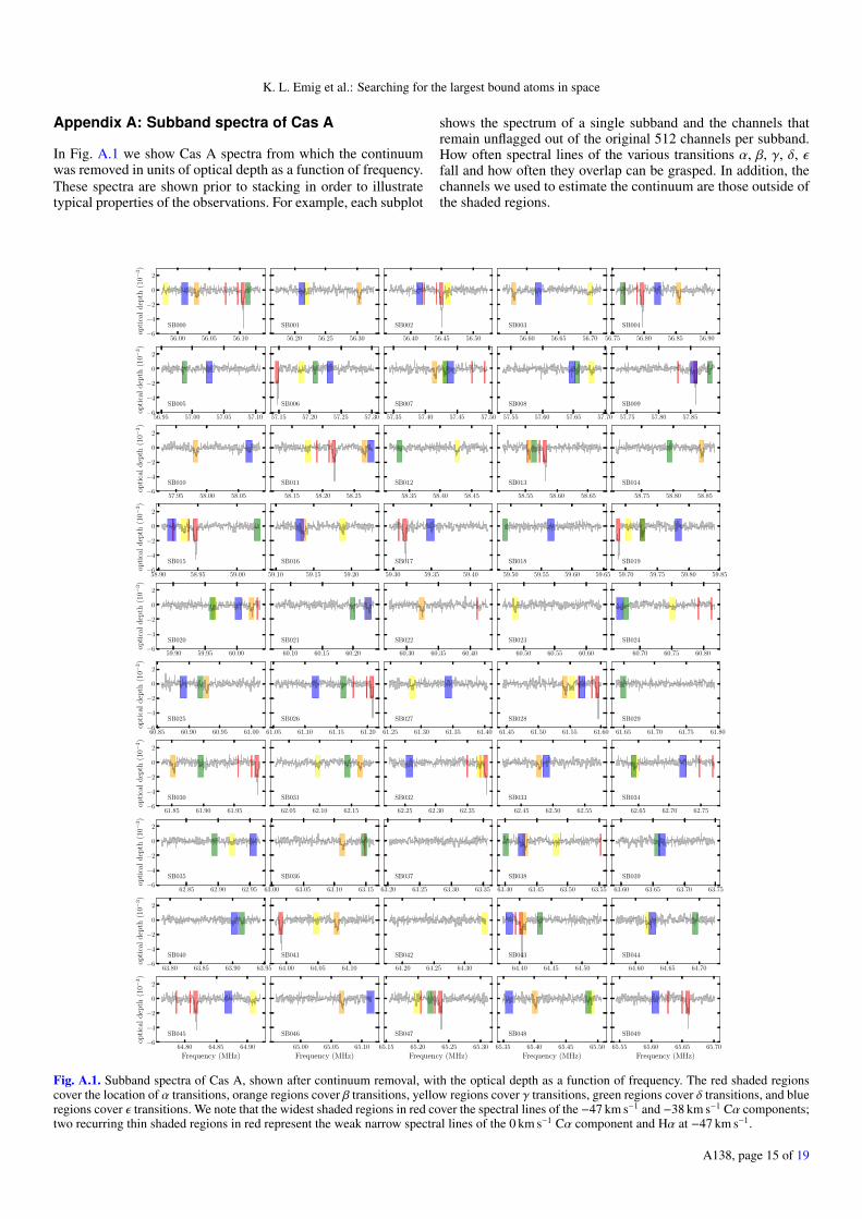
K. L. Emig et al.: Searching for the largest bound atoms in space

Appendix A: Subband spectra of Cas A

In Fig. A.1 we show Cas A spectra from which the continuumwas removed in units of optical depth as a function of frequency.These spectra are shown prior to stacking in order to illustratetypical properties of the observations. For example, each subplot

shows the spectrum of a single subband and the channels thatremain unflagged out of the original 512 channels per subband.How often spectral lines of the various transitions α, β, γ, δ, εfall and how often they overlap can be grasped. In addition, thechannels we used to estimate the continuum are those outside ofthe shaded regions.

56.00 56.05 56.10−6

−4

−2

0

2

opti

cal

dep

th(1

0−3)

SB000

56.20 56.25 56.30

SB001

56.40 56.45 56.50

SB002

56.60 56.65 56.70

SB003

56.75 56.80 56.85 56.90

SB004

56.95 57.00 57.05 57.10−6

−4

−2

0

2

opti

cal

dep

th(1

0−3)

SB005

57.15 57.20 57.25 57.30

SB006

57.35 57.40 57.45 57.50

SB007

57.55 57.60 57.65 57.70

SB008

57.75 57.80 57.85

SB009

57.95 58.00 58.05−6

−4

−2

0

2

opti

cal

dep

th(1

0−3)

SB010

58.15 58.20 58.25

SB011

58.35 58.40 58.45

SB012

58.55 58.60 58.65

SB013

58.75 58.80 58.85

SB014

58.90 58.95 59.00−6

−4

−2

0

2

opti

cal

dep

th(1

0−3)

SB015

59.10 59.15 59.20

SB016

59.30 59.35 59.40

SB017

59.50 59.55 59.60 59.65

SB018

59.70 59.75 59.80 59.85

SB019

59.90 59.95 60.00−6

−4

−2

0

2

opti

cal

dep

th(1

0−3)

SB020

60.10 60.15 60.20

SB021

60.30 60.35 60.40

SB022

60.50 60.55 60.60

SB023

60.70 60.75 60.80

SB024

60.85 60.90 60.95 61.00−6

−4

−2

0

2

opti

cal

dep

th(1

0−3)

SB025

61.05 61.10 61.15 61.20

SB026

61.25 61.30 61.35 61.40

SB027

61.45 61.50 61.55 61.60

SB028

61.65 61.70 61.75 61.80

SB029

61.85 61.90 61.95−6

−4

−2

0

2

opti

cal

dep

th(1

0−3)

SB030

62.05 62.10 62.15

SB031

62.25 62.30 62.35

SB032

62.45 62.50 62.55

SB033

62.65 62.70 62.75

SB034

62.85 62.90 62.95−6

−4

−2

0

2

opti

cal

dep

th(1

0−3)

SB035

63.00 63.05 63.10 63.15

SB036

63.20 63.25 63.30 63.35

SB037

63.40 63.45 63.50 63.55

SB038

63.60 63.65 63.70 63.75

SB039

63.80 63.85 63.90 63.95−6

−4

−2

0

2

opti

cal

dep

th(1

0−3)

SB040

64.00 64.05 64.10

SB041

64.20 64.25 64.30

SB042

64.40 64.45 64.50

SB043

64.60 64.65 64.70

SB044

64.80 64.85 64.90

Frequency (MHz)

−6

−4

−2

0

2

opti

cal

dep

th(1

0−3)

SB045

65.00 65.05 65.10

Frequency (MHz)

SB046

65.15 65.20 65.25 65.30

Frequency (MHz)

SB047

65.35 65.40 65.45 65.50

Frequency (MHz)

SB048

65.55 65.60 65.65 65.70

Frequency (MHz)

SB049

Fig. A.1. Subband spectra of Cas A, shown after continuum removal, with the optical depth as a function of frequency. The red shaded regionscover the location of α transitions, orange regions cover β transitions, yellow regions cover γ transitions, green regions cover δ transitions, and blueregions cover ε transitions. We note that the widest shaded regions in red cover the spectral lines of the −47 km s−1 and −38 km s−1 Cα components;two recurring thin shaded regions in red represent the weak narrow spectral lines of the 0 km s−1 Cα component and Hα at −47 km s−1.

A138, page 15 of 19

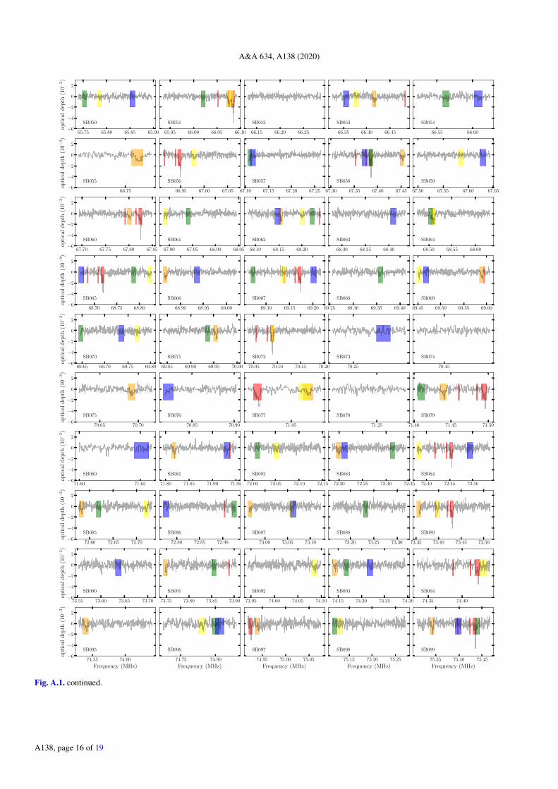
A&A 634, A138 (2020)

65.75 65.80 65.85 65.90−6

−4

−2

0

2

opti

cal

dep

th(1

0−3)

SB050

65.95 66.00 66.05 66.10

SB051

66.15 66.20 66.25

SB052

66.35 66.40 66.45

SB053

66.55 66.60

SB054

66.75−6

−4

−2

0

2

opti

cal

dep

th(1

0−3)

SB055

66.95 67.00 67.05

SB056

67.10 67.15 67.20 67.25

SB057

67.30 67.35 67.40 67.45

SB058

67.50 67.55 67.60 67.65

SB059

67.70 67.75 67.80 67.85−6

−4

−2

0

2

opti

cal

dep

th(1

0−3)

SB060

67.90 67.95 68.00 68.05

SB061

68.10 68.15 68.20

SB062

68.30 68.35 68.40

SB063

68.50 68.55 68.60

SB064

68.70 68.75 68.80−6

−4

−2

0

2

opti

cal

dep

th(1

0−3)

SB065

68.90 68.95 69.00

SB066

69.10 69.15 69.20

SB067

69.25 69.30 69.35 69.40

SB068

69.45 69.50 69.55 69.60

SB069

69.65 69.70 69.75 69.80−6

−4

−2

0

2

opti

cal

dep

th(1

0−3)

SB070

69.85 69.90 69.95 70.00

SB071

70.05 70.10 70.15 70.20

SB072

70.25

SB073

70.45

SB074

70.65 70.70−6

−4

−2

0

2

opti

cal

dep

th(1

0−3)

SB075

70.85 70.90

SB076

71.05

SB077

71.25

SB078

71.40 71.45 71.50

SB079

71.60 71.65−6

−4

−2

0

2

opti

cal

dep

th(1

0−3)

SB080

71.80 71.85 71.90 71.95

SB081

72.00 72.05 72.10 72.15

SB082

72.20 72.25 72.30 72.35

SB083

72.40 72.45 72.50

SB084

72.60 72.65 72.70−6

−4

−2

0

2

opti

cal

dep

th(1

0−3)

SB085

72.80 72.85 72.90

SB086

73.00 73.05 73.10

SB087

73.20 73.25 73.30

SB088

73.35 73.40 73.45 73.50

SB089

73.55 73.60 73.65 73.70−6

−4

−2

0

2

opti

cal

dep

th(1

0−3)

SB090

73.75 73.80 73.85 73.90

SB091

73.95 74.00 74.05 74.10

SB092

74.15 74.20 74.25 74.30

SB093

74.35 74.40

SB094

74.55 74.60

Frequency (MHz)

−6

−4

−2

0

2

opti

cal

dep

th(1

0−3)

SB095

74.75 74.80

Frequency (MHz)

SB096

74.95 75.00 75.05

Frequency (MHz)

SB097

75.15 75.20 75.25

Frequency (MHz)

SB098

75.35 75.40 75.45

Frequency (MHz)

SB099

Fig. A.1. continued.

A138, page 16 of 19

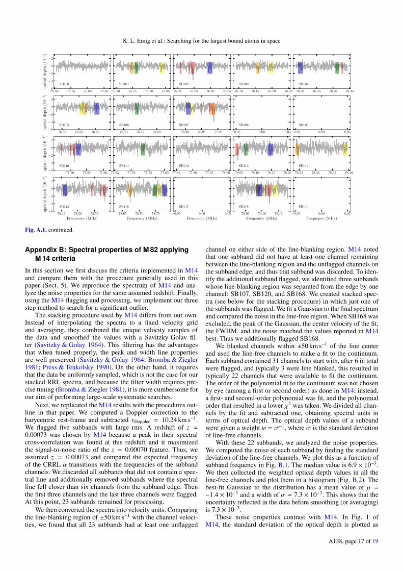
K. L. Emig et al.: Searching for the largest bound atoms in space

75.50 75.55 75.60 75.65−6

−4

−2

0

2

opti

cal

dep

th(1

0−3)

SB100

75.70 75.75 75.80 75.85

SB101

75.90 75.95 76.00 76.05

SB102

76.10 76.15 76.20 76.25

SB103

76.30 76.35 76.40 76.45

SB104

76.50 76.55 76.60−6

−4

−2

0

2

opti

cal

dep

th(1

0−3)

SB105

76.70 76.75 76.80

SB106

76.90 76.95 77.00

SB107

−0.05 0.00 0.05

SB108

−0.05 0.00 0.05

SB109

77.50 77.55 77.60−6

−4

−2

0

2

opti

cal

dep

th(1

0−3)

SB110

77.65 77.70 77.75 77.80

SB111

77.85 77.90 77.95 78.00

SB112

78.05 78.10 78.15 78.20

SB113

78.25 78.30 78.35 78.40

SB114

78.45 78.50 78.55

Frequency (MHz)

−6

−4

−2

0

2

opti

cal

dep

th(1

0−3)

SB115

78.65 78.70 78.75

Frequency (MHz)

SB116

−0.05 0.00 0.05

Frequency (MHz)

SB117

79.05 79.10 79.15

Frequency (MHz)

SB118

−0.05 0.00 0.05

Frequency (MHz)

SB119

Fig. A.1. continued.

Appendix B: Spectral properties of M 82 applyingM 14 criteria

In this section we first discuss the criteria implemented in M14and compare them with the procedure generally used in thispaper (Sect. 5). We reproduce the spectrum of M14 and ana-lyze the noise properties for the same assumed redshift. Finally,using the M14 flagging and processing, we implement our threestep method to search for a significant outlier.

The stacking procedure used by M14 differs from our own.Instead of interpolating the spectra to a fixed velocity gridand averaging, they combined the unique velocity samples ofthe data and smoothed the values with a Savitzky-Golav fil-ter (Savitzky & Golay 1964). This filtering has the advantagesthat when tuned properly, the peak and width line propertiesare well preserved (Savitzky & Golay 1964; Bromba & Ziegler1981; Press & Teukolsky 1990). On the other hand, it requiresthat the data be uniformly sampled, which is not the case for ourstacked RRL spectra, and because the filter width requires pre-cise tuning (Bromba & Ziegler 1981), it is more cumbersome forour aim of performing large-scale systematic searches.

Next, we replicated the M14 results with the procedures out-line in that paper. We computed a Doppler correction to thebarycentric rest-frame and subtracted vDoppler = 10.24 km s−1.We flagged five subbands with large rms. A redshift of z =0.00073 was chosen by M14 because a peak in their spectralcross-correlation was found at this redshift and it maximizedthe signal-to-noise ratio of the z = 0.00070 feature. Thus, weassumed z = 0.00073 and compared the expected frequencyof the CRRL α transitions with the frequencies of the subbandchannels. We discarded all subbands that did not contain a spec-tral line and additionally removed subbands where the spectralline fell closer than six channels from the subband edge. Thenthe first three channels and the last three channels were flagged.At this point, 23 subbands remained for processing.

We then converted the spectra into velocity units. Comparingthe line-blanking region of ±50 km s−1 with the channel veloci-ties, we found that all 23 subbands had at least one unflagged

channel on either side of the line-blanking region. M14 notedthat one subband did not have at least one channel remainingbetween the line-blanking region and the unflagged channels onthe subband edge, and thus that subband was discarded. To iden-tify the additional subband flagged, we identified three subbandswhose line-blanking region was separated from the edge by onechannel: SB107, SB120, and SB168. We created stacked spec-tra (see below for the stacking procedure) in which just one ofthe subbands was flagged. We fit a Gaussian to the final spectrumand compared the noise in the line-free region. When SB168 wasexcluded, the peak of the Gaussian, the center velocity of the fit,the FWHM, and the noise matched the values reported in M14best. Thus we additionally flagged SB168.

We blanked channels within ±50 km s−1 of the line centerand used the line-free channels to make a fit to the continuum.Each subband contained 31 channels to start with, after 6 in totalwere flagged, and typically 3 were line blanked, this resulted intypically 22 channels that were available to fit the continuum.The order of the polynomial fit to the continuum was not chosenby eye (among a first or second order) as done in M14; instead,a first- and second-order polynomial was fit, and the polynomialorder that resulted in a lower χ2 was taken. We divided all chan-nels by the fit and subtracted one, obtaining spectral units interms of optical depth. The optical depth values of a subbandwere given a weight w = σ−1, where σ is the standard deviationof line-free channels.

With these 22 subbands, we analyzed the noise properties.We computed the noise of each subband by finding the standarddeviation of the line-free channels. We plot this as a function ofsubband frequency in Fig. B.1. The median value is 6.9 × 10−3.We then collected the weighted optical depth values in all theline-free channels and plot them in a histogram (Fig. B.2). Thebest-fit Gaussian to the distribution has a mean value of µ =−1.4 × 10−3 and a width of σ = 7.3 × 10−3. This shows that theuncertainty reflected in the data before smoothing (or averaging)is 7.3 × 10−3.

These noise properties contrast with M14. In Fig. 1 ofM14, the standard deviation of the optical depth is plotted as

A138, page 17 of 19

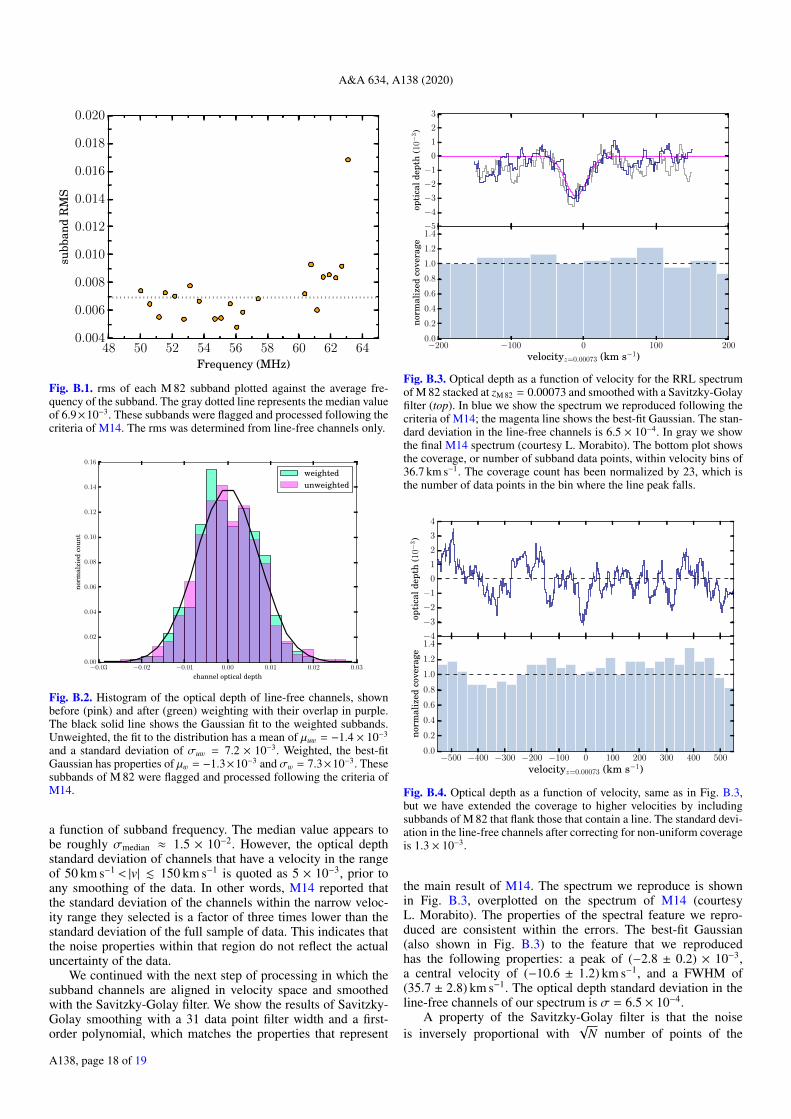
A&A 634, A138 (2020)

48 50 52 54 56 58 60 62 64Frequency (MHz)

0.004

0.006

0.008

0.010

0.012

0.014

0.016

0.018

0.020

subb

and

RM

S

Fig. B.1. rms of each M 82 subband plotted against the average fre-quency of the subband. The gray dotted line represents the median valueof 6.9×10−3. These subbands were flagged and processed following thecriteria of M14. The rms was determined from line-free channels only.

−0.03 −0.02 −0.01 0.00 0.01 0.02 0.03

channel optical depth

0.00

0.02

0.04

0.06

0.08

0.10

0.12

0.14

0.16

norm

alzi

edco

unt

weightedunweighted

Fig. B.2. Histogram of the optical depth of line-free channels, shownbefore (pink) and after (green) weighting with their overlap in purple.The black solid line shows the Gaussian fit to the weighted subbands.Unweighted, the fit to the distribution has a mean of µuw = −1.4 × 10−3

and a standard deviation of σuw = 7.2 × 10−3. Weighted, the best-fitGaussian has properties of µw = −1.3×10−3 and σw = 7.3×10−3. Thesesubbands of M 82 were flagged and processed following the criteria ofM14.

a function of subband frequency. The median value appears tobe roughly σmedian ≈ 1.5 × 10−2. However, the optical depthstandard deviation of channels that have a velocity in the rangeof 50 km s−1 < |v| . 150 km s−1 is quoted as 5 × 10−3, prior toany smoothing of the data. In other words, M14 reported thatthe standard deviation of the channels within the narrow veloc-ity range they selected is a factor of three times lower than thestandard deviation of the full sample of data. This indicates thatthe noise properties within that region do not reflect the actualuncertainty of the data.

We continued with the next step of processing in which thesubband channels are aligned in velocity space and smoothedwith the Savitzky-Golay filter. We show the results of Savitzky-Golay smoothing with a 31 data point filter width and a first-order polynomial, which matches the properties that represent

−5

−4

−3

−2

−1

0

1

2

3

opti

cald

epth

(10−

3)

−200 −100 0 100 200

velocityz=0.00073 (km s−1)

0.0

0.2

0.4

0.6

0.8

1.0

1.2

1.4

norm

aliz

edco

vera

ge

Fig. B.3. Optical depth as a function of velocity for the RRL spectrumof M 82 stacked at zM 82 = 0.00073 and smoothed with a Savitzky-Golayfilter (top). In blue we show the spectrum we reproduced following thecriteria of M14; the magenta line shows the best-fit Gaussian. The stan-dard deviation in the line-free channels is 6.5 × 10−4. In gray we showthe final M14 spectrum (courtesy L. Morabito). The bottom plot showsthe coverage, or number of subband data points, within velocity bins of36.7 km s−1. The coverage count has been normalized by 23, which isthe number of data points in the bin where the line peak falls.

−4

−3

−2

−1

0

1

2

3

4

opti

cald

epth

(10−

3)

−500 −400 −300 −200 −100 0 100 200 300 400 500

velocityz=0.00073 (km s−1)

0.0

0.2

0.4

0.6

0.8

1.0

1.2

1.4

norm

aliz

edco

vera

ge

Fig. B.4. Optical depth as a function of velocity, same as in Fig. B.3,but we have extended the coverage to higher velocities by includingsubbands of M 82 that flank those that contain a line. The standard devi-ation in the line-free channels after correcting for non-uniform coverageis 1.3 × 10−3.

the main result of M14. The spectrum we reproduce is shownin Fig. B.3, overplotted on the spectrum of M14 (courtesyL. Morabito). The properties of the spectral feature we repro-duced are consistent within the errors. The best-fit Gaussian(also shown in Fig. B.3) to the feature that we reproducedhas the following properties: a peak of (−2.8 ± 0.2) × 10−3,a central velocity of (−10.6 ± 1.2) km s−1, and a FWHM of(35.7 ± 2.8) km s−1. The optical depth standard deviation in theline-free channels of our spectrum is σ = 6.5 × 10−4.

A property of the Savitzky-Golay filter is that the noiseis inversely proportional with

√N number of points of the

A138, page 18 of 19

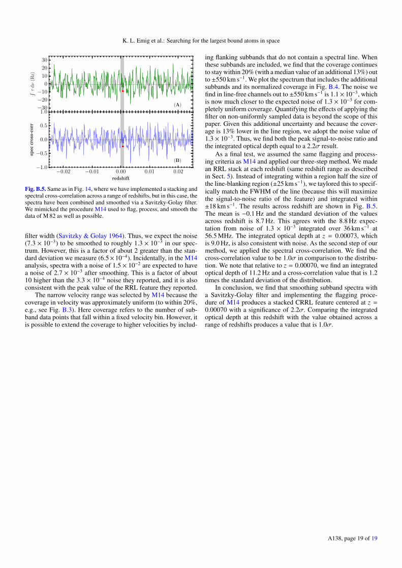
K. L. Emig et al.: Searching for the largest bound atoms in space

−30

−20

−10

0

10

20

30

∫τ

dν

(Hz)

(A)

−0.02 −0.01 0.00 0.01 0.02redshift

−1.0

−0.5

0.0

0.5

1.0

spec

cros

s-co

rr

(B)

Fig. B.5. Same as in Fig. 14, where we have implemented a stacking andspectral cross-correlation across a range of redshifts, but in this case, thespectra have been combined and smoothed via a Savitzky-Golay filter.We mimicked the procedure M14 used to flag, process, and smooth thedata of M 82 as well as possible.

filter width (Savitzky & Golay 1964). Thus, we expect the noise(7.3 × 10−3) to be smoothed to roughly 1.3 × 10−3 in our spec-trum. However, this is a factor of about 2 greater than the stan-dard deviation we measure (6.5×10−4). Incidentally, in the M14analysis, spectra with a noise of 1.5 × 10−2 are expected to havea noise of 2.7 × 10−3 after smoothing. This is a factor of about10 higher than the 3.3 × 10−4 noise they reported, and it is alsoconsistent with the peak value of the RRL feature they reported.

The narrow velocity range was selected by M14 because thecoverage in velocity was approximately uniform (to within 20%,e.g., see Fig. B.3). Here coverage refers to the number of sub-band data points that fall within a fixed velocity bin. However, itis possible to extend the coverage to higher velocities by includ-

ing flanking subbands that do not contain a spectral line. Whenthese subbands are included, we find that the coverage continuesto stay within 20% (with a median value of an additional 13%) outto ±550 km s−1. We plot the spectrum that includes the additionalsubbands and its normalized coverage in Fig. B.4. The noise wefind in line-free channels out to ±550 km s−1 is 1.1× 10−3, whichis now much closer to the expected noise of 1.3 × 10−3 for com-pletely uniform coverage. Quantifying the effects of applying thefilter on non-uniformly sampled data is beyond the scope of thispaper. Given this additional uncertainty and because the cover-age is 13% lower in the line region, we adopt the noise value of1.3 × 10−3. Thus, we find both the peak signal-to-noise ratio andthe integrated optical depth equal to a 2.2σ result.

As a final test, we assumed the same flagging and process-ing criteria as M14 and applied our three-step method. We madean RRL stack at each redshift (same redshift range as describedin Sect. 5). Instead of integrating within a region half the size ofthe line-blanking region (±25 km s−1), we taylored this to specif-ically match the FWHM of the line (because this will maximizethe signal-to-noise ratio of the feature) and integrated within±18 km s−1. The results across redshift are shown in Fig. B.5.The mean is −0.1 Hz and the standard deviation of the valuesacross redshift is 8.7 Hz. This agrees with the 8.8 Hz expec-tation from noise of 1.3 × 10−3 integrated over 36 km s−1 at56.5 MHz. The integrated optical depth at z = 0.00073, whichis 9.0 Hz, is also consistent with noise. As the second step of ourmethod, we applied the spectral cross-correlation. We find thecross-correlation value to be 1.0σ in comparison to the distribu-tion. We note that relative to z = 0.00070, we find an integratedoptical depth of 11.2 Hz and a cross-correlation value that is 1.2times the standard deviation of the distribution.

In conclusion, we find that smoothing subband spectra witha Savitzky-Golay filter and implementing the flagging proce-dure of M14 produces a stacked CRRL feature centered at z =0.00070 with a significance of 2.2σ. Comparing the integratedoptical depth at this redshift with the value obtained across arange of redshifts produces a value that is 1.0σ.

A138, page 19 of 19