Electronic copy available at: http://ssrn.com/abstract=2158703

Searching for a Common Factor

in Public and Private Real Estate Returns

Andrew Ang,* Neil Nabar,† and Samuel Wald‡

Abstract

We introduce a methodology to estimate common real estate returns and cycles across public and

private real estate markets. We first place REIT indices and direct real estate—NCREIF appraisal-based

and transaction-based indices (NPI and NTBI)—on a comparable basis by adjusting for leverage and

sector. We extract a common real estate factor, which is allowed to be persistent, from all these

markets. Individual real estate indices load on this common factor and they also are driven by

persistent, idiosyncratic shocks. The common real estate factor is procyclical and has low correlations

with standard systematic factors. Short-run idiosyncratic deviations from the common real estate factor

load on several capital market factors for REITs and on liquidity factors for direct real estate.

This Version: 10-11-2012

* Ann F. Kaplan Professor of Business, Columbia Business School, New York, NY † Research Analyst, Fidelity Investments, Boston, MA, Corresponding author, Neil.Nabar@fmr.com ‡ Portfolio Manager, Fidelity Investments, Boston MA

Electronic copy available at: http://ssrn.com/abstract=2158703

1. INTRODUCTION

Are real estate investment trusts (REITs) and direct real estate ownership similar or different? On the

one hand, both involve investing in physical buildings and land, which generate cash flows. Pagliari,

Scherer, and Monopoli [2003, 2005] suggest that after adjusting REITs and direct real estate indices for

leverage and sector composition, and also adjusting direct real estate returns for appraisal smoothing,

REITs and direct ownership have similar risk and return characteristics. Other authors have shown there

are important differences between REITs and direct real estate returns. For example, direct real estate

transactions lead direct real estate appraisals, and there are significant lead-lag patterns between REITs

and direct real estate returns.1 Some of these differences persist even after taking into account the

different sector and leverage composition of REITs and direct real estate returns.

We study the long-run commonality and short-run differences between REITs and direct real estate

returns. Although REITs are securitized, REITs and direct real estate returns should be driven by common

fundamentals in the long run since both involve ownership of real estate. Carlson, Titman, and Tiu

[2010] develop a model based on different costs of capital in which public and private real estate

markets move together in the long run, but in the short run, REITs and direct real estate price

movements can diverge.

In the short run, REITs and direct real estate returns diverge through vehicle-specific shocks. Since REITs

provide immediate liquidity and trade on centralized exchanges where other equities trade, they are

exposed to systematic equity market factors. Clayton and MacKinnon [2001], for example, argue that

REITs have significant exposure to value and small-cap factors. REITs are widely held and so may be

buffeted by investor sentiment and noise traders, which DeLong, Shleifer, Summers, and Waldmann

[1990], Hong, Scheinkman, and Xiong [2006], and others argue are significant influences on publicly

traded stock markets. By contrast, direct real estate investing involves less frequent transactions and

appraisal-based pricing tends to smooth returns over time. Direct real estate is then exposed to liquidity

smoothing effects which do not affect REITs. Over the long run, these effects could cancel out, so that

both REITs and direct real estate returns are exposed to the same common drivers and thus move

together.

Our analysis proceeds in three parts. First, we follow Pagliari, Scherer, and Monopoli [2005] and Li,

Mooradian, and Yang [2009], among others, and place REIT and direct real estate returns on a

comparable basis so that they have the same leverage and sector composition. We refer to the raw REIT

1 See, for example, Gyourko and Keim [1992], Barkham and Geltner [1995], and Oikarinen, Hoesli, and Serrano [2011].

2

and direct real estate returns adjusted this way as comparable returns. Unlike Pagliari, Scherer, and

Monopoli [2005], we do not adjust for autocorrelations or volatility induced by the appraisal process.

Rather, we preserve these idiosyncratic properties because they are specific to a particular index, and

we wish to characterize how each index differs from the components that are common across REIT and

direct real estate markets.

Second, we estimate a common factor across REIT and direct real estate returns using a latent

components model. We filter the common real estate factor from the observed comparable REIT and

direct real estate returns. The model attributes some portion of the movements of a particular real

estate index as shared across all indexes, but some portion is specific to that index. Both the common

and idiosyncratic components are allowed to be autocorrelated. Our estimation methodology handles

different starting dates of each index.

Finally, we characterize the dynamics of the common real estate factor and examine how the index-

specific components move relative to the common factor. This allows us to explicitly link the sources of

difference between the common real estate factor and the underlying characteristics of the various real

estate investment vehicles.

Our approach is related to a number of papers which investigate the lead-lag relationships between

REITs and direct real estate, especially within cointegrated systems.2 Our approach is different because

we work directly with returns, which are I(0), rather than with a total return index, which is I(1). This

makes our work comparable with the majority of finance studies which directly model returns. By

assuming a factor model, we also impose economic restrictions on the sources of the shocks to each real

estate market—that they must come from common sources or idiosyncratic sources. Thus, the main

advantage is that our model highlights the common real estate factor and treats each real estate market

as directly exposed to the common factor. Cointegration models, in contrast, employ an unconstrained

covariance matrix and estimate a common trend by finding a linear combination of the I(1) series that is

stationary rather than decomposing common and idiosyncratic shocks.

Working directly with returns rather than I(1) variables also makes our work similar to standard factor

models such as the CAPM or APT and makes our model comparable to the earlier literature by

Goetzmann and Ibbotson [1990], Giliberto [1990], and Ling and Naranjo [1999]. However, these authors

do not allow for any persistence. In our model both the systematic and idiosyncratic components can be

autocorrelated, and we empirically find that persistence is high for the common real estate factor and

2 See, among others, Meyer and Webb [1994]; Geltner and Kluger [1998]; Pagliari, Scherer, and Monopoli [2005]; Hoesli and Serrano [2007]; Fuss, Morawski, and Rehkugler [2008]); Li, Mooradian, and Yang [2009]; Oikarinen, Hoesli, and Serrano [2011]; and Stefek and Suryanarayanan [2011]

3

the direct real estate idiosyncratic components. Thus, our model also captures the smoothing effects of

Geltner [1991] and Ross and Zisler [1991], but allows the common and idiosyncratic smoothing effects

to be estimated rather than needing to be directly observed.

2. DATA

We adjust the REIT returns to be comparable to direct real estate on the basis of sector and leverage

adjustments following Pagliari, Scherer, and Monopoli [2003, 2005].

For publicly traded real estate, we take REITs from the CRSP/Ziman Real Estate Data Series. The

CRSP/Ziman stocks are linked with CRSP for returns and with Compustat for financial statement data. As

a starting point for publicly listed real estate returns, we construct a value-weighted index of REIT

returns from this combined dataset. For privately held real estate returns, we use two indices based on

data from the National Council of Real Estate Fiduciaries (NCREIF). The first is the appraisal-based

Property Index (NPI). Appraisals are calculated based on factors that are already in place and are not

instantaneous and are therefore lagging. The second is the NCREIF Transaction Based Index (NTBI),

which is based on properties in the NPI that were sold.3

As of December 1980, there were 54 REITs with an aggregate market capitalization of $1.8 billion in the

CRSP/Ziman equity-only series, compared to $1.9 billion in privately held properties in the NCREIF

database. In the early 1990s, the number and market value of REITs as well as the market value of

private market transactions increased dramatically. During the recovery from the savings and loan crisis

of the late 1980s and early 1990s, the real estate industry recapitalized and investment in both REITs

and direct real estate increased. The number of REITs peaked around 200 in 1998, and REIT

capitalization reached a maximum above $430 billion in 2007. The market value of the NPI posted a high

close to $340 billion in 2008. Since then, the number of REITs has fallen to 133 with a $370 billion

capitalization in December 2011, compared to $280 billion in privately held real estate in the NPI and

NTBI series.4

3 The NTBI is calculated in two stages. First, for all properties sold in the quarter, NCREIF calculates the average ratio of the sales price divided by the appraisal, lagged two quarters. Second, this ratio is multiplied by the NPI level, also lagged two quarters, to convert the result into the NTBI transaction-based price index. The lagged appraisal is used instead of the current appraisal because the appraisal price may be influenced by a subsequent sale within two quarters. 4 Source: Authors based on CRSP/Ziman and NCREIF data.

4

2.1 Leverage Adjustments

Although individual properties within the NPI and NTBI have leverage associated with them, NPI and

NTBI returns are reported on an unlevered basis. REIT returns, on the other hand, represent the equity

return of leveraged properties. During the past 30 years, REIT leverage—debt and preferred equity

divided by enterprise value—has averaged 43%, and annual interest expenses have ranged from just

under 6% to almost 9%.5

We delever the REIT returns to make them comparable to the NCREIF returns following Pagliari, Scherer,

and Monopoli [2003, 2005]. Using the most recent balance sheet data on a monthly basis, we compute a

leverage ratio for each REIT:

Debt + Preferred Equity

Leverage Ratio = ,Debt + Preferred Equity + Equity Market Capitalization

(1)

where the equity market capitalization is computed using common equity, and we take book values for

the preferred stock and debt. We compute an annualized interest cost per month for each REIT using

the formula:

1 1

1 12 2

Interest & Preferred Cost

LTM Interest Expense + LTM Preferred Dividends = ,

(Debt Preferred Equity ) (Debt Preferred Equity )t t t t− −+ + + (2)

which takes the interest and preferred dividends paid over the last 12 months divided by the average

amount of preferred equity and debt over the last 12 months. We use a one-year window to estimate

the interest rate of debt to control for the effects of refinancing.

Using the leverage ratio and interest cost in equations (1) and (2), respectively, we compute a monthly

delevered REIT return:

Delevered REIT Return = REIT Return (1- Leverage Ratio)

Interest Expense+ Leverage Ratio,

12

×

× (3)

The delevered monthly REIT returns are converted to the quarterly frequency to match the quarterly

frequency of the NPI and NTBI series.

5 Source: Authors based on CRSP/Ziman data.

5

Exhibit 1 shows that from January 1994 to December 2011, the raw REIT average return per quarter is

2.53%, with a standard deviation of 13.07%. Taking leverage into account lowers the average quarterly

return to 1.14%, with a standard deviation of 5.15%. Thus, adjusting for leverage has a substantial effect

on average returns and volatility—a crucial distinction between REITs and reported direct real estate

returns.

EXHIBIT 1

Quarterly Returns, Standard Deviations, and Serial Correlations of Public and Private Real Estate

Source: Authors based on CRSP/Ziman and NCREIF data.

2.2 Sector Adjustments

REIT and NCREIF returns have different sector compositions. REITs primarily fall into the four “core” real

estate sectors of apartment, retail, office, and industrial, although other sectors are gaining

representation.6 By contrast, given NCREIF’s institutional focus, NPI and NTBI include only the four core

real estate sectors plus hotels. To place REITs, NPI, and NTBI on the same sector basis, we consider the

four core real estate sectors without hotels.7 Retail REITs have the largest weight in the CRSP/Ziman REIT

series. Apartment, office, and industrial REITs have stayed in 5%–10% bands around their current

weights. Historically, office and retail have been the largest weights in the NCREIF indices. Retail

6 Historically at least 80% of the total REIT capitalization was in these sectors, but that weighting has fallen to about 60% in recent years as new sectors—including healthcare, data center, storage, timber, and others—have converted to REIT status and/or gained investor attention. 7 We also exclude hotels because of their small weight in the NPI—less than 5% at any time—and their relatively infrequent transactions.

Serial Correlation

5 year 10 year Since 1994Available

History Since 1994 Available

HistoryAvailable

HistoryREIT 2.53% 3.96% 3.40% 3.46% 13.07% 11.51% 0.14NPI 0.84% 2.01% 2.25% 2.06% 2.43% 2.22% 0.78NTBI 0.62% 2.34% 2.74% 2.74% 5.74% 5.74% -0.12

REIT (leverage adjusted only) 1.14% 2.37% 2.36% 2.71% 5.15% 4.79% 0.07

Comparable REIT 1.16% 2.38% 2.41% 2.78% 4.99% 4.51% 0.06Comparable NPI 0.98% 2.19% 2.31% 2.28% 2.24% 1.98% 0.77Comparable NTBI 0.47% 2.41% 2.64% 2.64% 5.49% 5.49% -0.15

Note: Available history starts in Q1 1994 for NTBI and Q2 1980 for other series. All series end in Q4 2011.

Average Quarterly ReturnsQuarterly Standard

Deviation

6

gradually moved from the 40% in 1994 to 22% today as the supply of other property types grew much

faster than retail, while some retail types—especially malls—moved into the REIT format.8

Exhibit 2 shows the sector composition of our core REIT and NPI/NTBI series as of December 2011. REITs

are much more heavily weighted towards retail, at 46%, while the NPI/NTBI property-type mix is more

balanced, with a 22% weight in retail. Offices, at 36%, account for a larger proportion of the direct

property index, compared to the REITs weight of 18%.

EXHIBIT 2

REIT and NPI/NTBI Core Property-Type Weights as of 12/31/2011

Source: Authors based on CRSP/Ziman and NCREIF data.

To construct a comparable REIT return series, we weight monthly returns of REITs in the four core

property types (apartment, retail, office, and industrial) by total capitalization (debt plus preferred stock

plus equity). To construct the comparable NPI and comparable NTBI returns, we weight the quarterly

NPI and NTBI returns for each property type and by the weights of each property type in the comparable

REIT index.

Exhibit 1 also reports summary statistics of the comparable REIT, NPI, and NTBI series. Taking sector

composition into account does not significantly change the returns from the delevered REIT series or the

raw NPI and NTBI series. For example, the mean and standard deviation per quarter of the delevered

REIT returns are 2.36% and 5.15%, respectively, from 1994 to 2011. Allocating the REIT series into the

core property types changes the mean and standard deviation per quarter to 2.41% and 4.99%,

respectively. Similarly, weighting the NPI and NTBI with the same sector weights as the core property

8 Source: Authors based on CRSP/Ziman and NCREIF data.

Apartment25%

Industrial11%

Office18%

Retail46%

REITs Core Property Type Sector Mix

Apartment27%

Industrial15%Office

36%

Retail22%

NPI/NTBI Core Property Type Mix

7

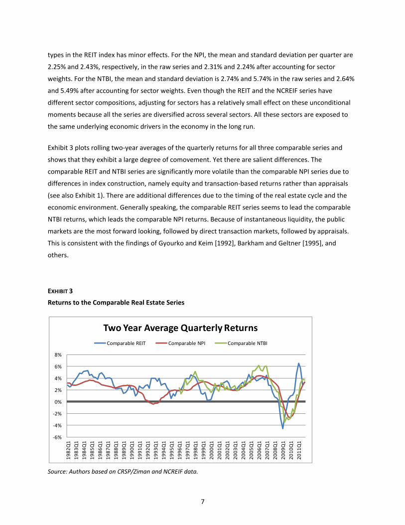
types in the REIT index has minor effects. For the NPI, the mean and standard deviation per quarter are

2.25% and 2.43%, respectively, in the raw series and 2.31% and 2.24% after accounting for sector

weights. For the NTBI, the mean and standard deviation is 2.74% and 5.74% in the raw series and 2.64%

and 5.49% after accounting for sector weights. Even though the REIT and the NCREIF series have

different sector compositions, adjusting for sectors has a relatively small effect on these unconditional

moments because all the series are diversified across several sectors. All these sectors are exposed to

the same underlying economic drivers in the economy in the long run.

Exhibit 3 plots rolling two-year averages of the quarterly returns for all three comparable series and

shows that they exhibit a large degree of comovement. Yet there are salient differences. The

comparable REIT and NTBI series are significantly more volatile than the comparable NPI series due to

differences in index construction, namely equity and transaction-based returns rather than appraisals

(see also Exhibit 1). There are additional differences due to the timing of the real estate cycle and the

economic environment. Generally speaking, the comparable REIT series seems to lead the comparable

NTBI returns, which leads the comparable NPI returns. Because of instantaneous liquidity, the public

markets are the most forward looking, followed by direct transaction markets, followed by appraisals.

This is consistent with the findings of Gyourko and Keim [1992], Barkham and Geltner [1995], and

others.

EXHIBIT 3

Returns to the Comparable Real Estate Series

Source: Authors based on CRSP/Ziman and NCREIF data.

-6%

-4%

-2%

0%

2%

4%

6%

8%

1982

Q1

1983

Q1

1984

Q1

1985

Q1

1986

Q1

1987

Q1

1988

Q1

1989

Q1

1990

Q1

1991

Q1

1992

Q1

1993

Q1

1994

Q1

1995

Q1

1996

Q1

1997

Q1

1998

Q1

1999

Q1

2000

Q1

2001

Q1

2002

Q1

2003

Q1

2004

Q1

2005

Q1

2006

Q1

2007

Q1

2008

Q1

2009

Q1

2010

Q1

2011

Q1

Two Year Average Quarterly ReturnsComparable REIT Comparable NPI Comparable NTBI

8

Exhibit 3 shows that during the early 1990s, real estate fundamentals were poor and recovering from an

oversupply of underlying properties. Very little capital was available to the real estate industry, and the

public markets provided capital for the industry to recapitalize. The ability to buy assets in the public

markets at favorable pricing helped REITs outperform the underlying property markets. During the late

1990s technology bubble, stock market investors were generally more focused on faster growing

companies, while steady industries like real estate were out of favor. Despite moderate fundamentals at

the underlying property level, the comparable REIT index underperformed the comparable NPI and NTBI

indices. In 2008–2009, the lack of liquidity impacted all forms of capital-intensive real estate as available

funding dried up. The overall message in Exhibit 3 is that the three series representing public and private

real estate markets have large underlying comovements reflecting common exposure to the underlying

economy. There are also important vehicle-specific idiosyncratic components. Estimating the

relationships between our three series to extract a common, underlying real estate factor is the focus of

the next section.

3. MODEL

We decompose a class of real estate, itr , into exposure to a common real estate factor, tf , and an

index-specific component, itg :

,it i t itr f gβ= + (4)

where iβ represents the loading of the real estate class, or investment vehicle, on the systematic real

estate factor, tf . We specify that the idiosyncratic component, itg , is orthogonal to the common real

estate factor, tf .

The common real estate factor, tf , follows:

1 ,t f f t f tf c fφ σ ε−= + + (5)

where ~tε N(0,1). The autocorrelation, fφ , allows for persistence in the common real estate factor.

The dynamics of the real estate index component, itg , follow:

, 1 ,it i i i t i itg c g uφ σ−= + + (6)

which also allows persistence through ϕi. We set ~itu IID N(0,1) to be independent of tε at all leads

9

and lags and also independent across series i.

Exhibit 4 illustrates the relation between the common real estate factor and the various real estate

series. Since we model returns in equations (4)–(6), the index level can be interpreted as the cumulated

return series. Movements in the real estate cycle correspond to the common real estate factor, tf . As

the model allows returns to be autocorrelated, it can capture the long swings in real estate markets

documented by many authors (see, for example, Wheaton [1999]). The individual real estate markets,

both public and private, follow the real estate cycle because they have exposure to the common real

estate factor through the factor loadings, iβ . The larger the factor loading, the more that real estate

market moves in sync with the real estate cycle, all other things being equal. The real estate indices do

not exactly follow the real estate cycle due to shocks that are specific to the market segment. These

shocks, itg , can themselves follow their own cycles, which are captured through the iφ terms. Since the

persistence of the idiosyncratic real estate market movements may not be the same as the common real

estate factor, the idiosyncratic cycles can partially offset, exacerbate, or sometimes completely cancel

the effect of the common real estate cycle.

EXHIBIT 4

Common Real Estate Factor and Real Estate Series

For illustrative purposes only.

10

The model allows for rich patterns in matching lead-lag patterns through implied cross- and auto-

correlations. For example, the cross-covariances of real estate market i and real estate market j are given

by

, ,cov( ) var( ),kit j t k i j f tr r fβ β φ− = (7)

where 2 2var( ) / (1 )t f ff σ φ= − . The cross-covariances of a given real estate class i are given by

2, ,cov( ) var( ) var( ),k k

it i t k i f t f itr r f gβ φ φ− = + (8)

where 2 2var( ) / (1 )it i ig σ φ= − .

The model can be interpreted as a factor model where tf is the common factor and itg are

idiosyncratic shocks specific to each real estate series. This makes our model similar to a CAPM or an

APT as well as the models estimated by Goetzmann and Ibbotson [1990], Giliberto [1990], and others.

However, there are two important differences: We allow for persistent common and idiosyncratic

factors, and our common factor is latent.

Geltner [1991], Ross and Zisler [1991], and many others develop methods to “unsmooth” direct real

estate returns. These methods implicitly involve modeling the private real estate return, which is the

illiquid asset, with loadings on contemporaneous and lagged asset returns that are assumed to be liquid

and have autocorrelations close to zero (see also Stefek and Suryanarayan [2011]). Standard smoothing

filters assume that the loadings decrease in absolute value as the lags increase. A similar formulation is

implied by our model. Since the common real estate factor, tf , is persistent, we have:

2 31 3 ...,it f i f t f i f t f i f tr k φ β σ ε φ β σ ε φ β σ ε− −= + + + + (9)

where the tε shocks are i.i.d. innovations to the common real estate factor in equation (5). Thus, the

exposure to a persistent real estate factor also induces smoothing in a particular real estate market. And

the model also allows the possibility of autocorrelated market-specific deviations away from the

common real estate factor.

We estimate the common real estate component, tf , by a Bayesian Gibbs sampling algorithm, which

we detail in the Appendix. The algorithm jointly estimates the common real estate factor and the

parameters of the model.

11

4. EMPIRICAL RESULTS

4.1 Parameter Estimates

Exhibit 5 reports parameter estimates of the model. The common real estate factor has an average

return of 1.89% per quarter. The common factor’s high quarterly autocorrelation (φf = 0.69) indicates

the strong influence of past observations and reflects the cyclical, trending nature of real estate. Factor-

loading betas above 1.0 for REIT and NTBI suggest that the market transaction-based vehicles have

greater exposure to the real estate factor, while the appraisal-based NPI has much lower exposure

(β = 0.37) to the real estate factor. Thus, market-based real estate transactions have greater exposure to

underlying real estate trends.

EXHIBIT 5

Parameter Estimates

Source: Authors based on CRSP/Ziman and NCREIF data.

The other model parameters reflect the series-specific idiosyncratic returns after subtracting the

common real estate factor from the three series. After this adjustment, REIT returns have no

autocorrelation (φ ≈ 0), which is expected for a public, forward-looking security, but the idiosyncratic

standard deviation is relatively high at 4.51% per quarter. In contrast, the NTBI returns are negatively

autocorrelated (φ = −0.34). This may reflect the noise and sampling bias inherent in the series, as only a

small fraction of properties trade during any given period (see comments by Goetzmann [1992]). We

find that the autocorrelation of the NPI is still high (φ = 0.59), even after adjusting for the common real

estate factor, which is also positively autocorrelated. Such predictable and persistent autocorrelation

reflects the smoothing inherent in returns that results from the appraisal process. This suggests a link to

Cannon and Cole [2011], who find that appraisals are off by 12% on average from transacted prices and

Mean Std Dev Mean Std Devcf 0.0189 0.0033 REIT c 0.0000 0.0002φf 0.6935 0.1212 REIT φ 0.0013 0.0615σf 0.0153 0.0029 REIT σ 0.0451 0.0039

NPI c -0.0026 0.0021NPI φ 0.5914 0.0862

Mean Std Dev NPI σ 0.0140 0.0009REIT β 1.2933 0.2734 NTBI c -0.0001 0.0013NPI β 0.3730 0.1025 NTBI φ -0.3386 0.0844

NTBI β 1.3337 0.2725 NTBI σ 0.0339 0.0030

Posterior

Factor Loadings

Idiosyncratic ReturnsCommon Real Estate Factor

Posterior

Posterior

12

lag prices in both rising and falling markets. According to Cannon and Cole, NPI appraisal error is

systematic and has a macro influence. Our results show that the persistence induced by this process is

even larger than the persistence from the general real estate cycle.

4.2 Common Real Estate Factor

Exhibit 6 plots the four-quarter moving average of the common real estate factor and the comparable

series. By construction, the real estate factor is a composite of the three underlying series, yet it is not

simply an equal-weighted combination of them. Rather, the algorithm allows each real estate market to

have different factor loadings and places more weight on the REIT and NTBI series (see Exhibit 5). Our

estimation is also able to extract the real estate factor in the early part of the sample even when the

NTBI series is not available. The common real estate factor captures the underlying trend of generally

positive quarterly returns in the real estate market during the past 30 years, with a slowdown in the late

1980s and early 1990s, extremely strong returns in the mid-2000s, and a steep decline in 2008–2009.

EXHIBIT 6

Returns to the Common Real Estate Factor and Comparable Real Estate Series

Source: Authors based on CRSP/Ziman and NCREIF data.

-8%

-6%

-4%

-2%

0%

2%

4%

6%

8%

10%

1981

Q1

1982

Q1

1983

Q1

1984

Q1

1985

Q1

1986

Q1

1987

Q1

1988

Q1

1989

Q1

1990

Q1

1991

Q1

1992

Q1

1993

Q1

1994

Q1

1995

Q1

1996

Q1

1997

Q1

1998

Q1

1999

Q1

2000

Q1

2001

Q1

2002

Q1

2003

Q1

2004

Q1

2005

Q1

2006

Q1

2007

Q1

2008

Q1

2009

Q1

2010

Q1

2011

Q1

1yr Quarterly Moving Average Returns of Real Estate Series

Common Real Estate Factor Comparable REIT

Comparable NPI Comparable NTBI

13

4.3 Common Real Estate Factor Innovations

We characterize how innovations to the common real estate factor move with macro, style, and liquidity

factors, all at the quarterly frequency. We start with the returns of the equity and bond markets,

proxied by the S&P 500 and Barclays Aggregate indices, to test for relations with the capital markets.

Since the demand for real estate is also related to aggregate activity in the real economy, we include

real GDP growth and the change in the Consumer Price Index (CPI). Finally, because real estate is a

capital-intensive business, we also include a credit spread variable, the difference between the yield on

BAA-rated corporate bonds and the yield on the 10-year Treasury. To characterize the real estate

market from an investment-style perspective, we look at several standard style factors: SMB, HML, and

MOM, respectively, which are the returns to small minus large cap stocks, value versus growth stocks,

and momentum constructed by Fama and French [1993] and Carhart [1997].

We also consider two liquidity variables. The first liquidity variable measures liquidity in stock markets.

Ibbotson, Chen, and Hu [2011] document that stocks sorted by turnover exhibit differences in returns.

Similarly, we rank stocks in the Russell 1000 Index monthly by turnover—defined as shares traded

divided by shares outstanding during the past 12 months—and then calculate the spread between the

one-month forward returns of the lowest quintile minus the returns of the highest quintile. This low

minus high turnover factor is the return to stock-level illiquidity. To measure the level of liquidity specific

to the real estate market more directly using NCREIF data, we calculate the percentage of properties in

the NPI that sold during a given quarter. These two factors have a cross-sectional correlation of only

0.02, suggesting that stock market liquidity and real estate liquidity are very different.

We regress innovations of the common real estate factor, which is defined as the innovation in equation

(5) above, and report the results in Exhibit 7.9 In the multivariate regression, the common real estate

factor loads positively and significantly on the S&P 500, indicating that it is procyclical. There is also a

large negative coefficient on the credit spread, which is not surprising given that real estate is a capital-

intensive asset class, and widening spreads are deleterious for the real estate industry. Real estate

return innovations are linked to stock market and real estate liquidity, but in different ways. Real estate

returns are negatively correlated with stock market liquidity. Consistent with Cannon and Cole [2011]

and others, there is a strong positive relation between real estate returns and real estate liquidity.

9 In the univariate regressions, the common real estate factor also loads significantly and positively on SMB, but negatively on stock market liquidity.

14

EXHIBIT 7

Regression Results: Common Real Estate Factor

Source: Authors based on Haver Analytics and Bloomberg data.

4.4 Specific Real Estate Market Innovations

We construct specific real estate market innovations taking the residuals in equation (6). Exhibit 8 plots

the two-year quarterly moving average of the innovations for each series. REIT innovations show the

greatest variability around the common real estate factor, and tend to lead the innovations in the NPI

and the NTBI. At turning points in the real estate cycle, REIT innovations move in opposite directions

from NPI innovations, trending significantly higher or lower during real estate booms and busts in 1990–

1994, 1998–2000, 2006–2008, and 2009–2011.

Exhibit 9 characterizes how real estate market innovations away from the common real estate market

cycle move. We run multivariate regressions on the innovations in the real estate series using the same

factors we used to analyze the common real estate factor.

We find that REIT innovations have several significant relationships with these exogenous factors,

loading positively on the S&P 500 and Barclays Aggregate indices as well as SMB and HML. Based on this

analysis, REITs provide investors with exposure to real estate through the common factor, as well as to

other macroeconomic and capital market—especially stock market—factors. Our results refine the

commonly held belief that REITs provide real estate exposure plus equity market exposure. These equity

P Value

S&P 500 Index 0.029 0.019

Barclays Aggregate 0.037 0.100

Change in Real GDP Growth 0.079 0.429

Change in CPI -0.065 0.631

Change in BAA – Treasury Spread -0.917 0.002

MOM 0.015 0.250

SMB 0.017 0.361

HML 0.019 0.238

Low Turnover – High Turnover -0.001 0.923

NPI Turnover 0.172 0.004

Note: Coefficients in bold are significant at 5% level.

BetaCommon Real Estate Factor Innovations

15

market exposures are a potential source of opportunity for active managers of REIT portfolios in the

short term.

EXHIBIT 8

Real Estate Series Innovations

Source: Authors.

EXHIBIT 9

Regression Results: REIT, NPI, and NTBI Innovations

Source: Authors based on Haver Analytics and Bloomberg data.

-4%

-3%

-2%

-1%

0%

1%

2%

3%

4%

5%

6%

1982

Q1

1983

Q1

1984

Q1

1985

Q1

1986

Q1

1987

Q1

1988

Q1

1989

Q1

1990

Q1

1991

Q1

1992

Q1

1993

Q1

1994

Q1

1995

Q1

1996

Q1

1997

Q1

1998

Q1

1999

Q1

2000

Q1

2001

Q1

2002

Q1

2003

Q1

2004

Q1

2005

Q1

2006

Q1

2007

Q1

2008

Q1

2009

Q1

2010

Q1

2011

Q1

2yr Quarterly Moving Average of Innovations

REIT Innovations NPI Innovations NTBI Innovations

Beta P Value Beta P Value Beta P Value

S&P 500 Index 0.234 0.000 0.007 0.630 -0.027 0.736

Barclays Aggregate 0.233 0.006 -0.019 0.520 -0.242 0.179

Change in Real GDP Growth -0.054 0.884 0.049 0.702 -0.733 0.368

Change in CPI 0.306 0.541 0.009 0.959 -0.510 0.579

Change in BAA – Treasury Spread -0.813 0.454 -0.883 0.019 -2.321 0.259

MOM 0.036 0.447 0.025 0.128 -0.130 0.165

SMB 0.289 0.000 -0.016 0.501 0.063 0.602

HML 0.155 0.011 0.024 0.253 -0.233 0.066

Low Turnover – High Turnover 0.038 0.316 -0.001 0.954 0.083 0.217

NPI Turnover -0.273 0.218 0.239 0.002 0.196 0.632

Note: Coefficients in bold are significant at 5% level.

REIT Innovations NPI Innovations NTBI InnovationsFactors

16

NPI innovations load on two factors, credit spreads and real estate market turnover. We believe this

offers several insights into the performance of the NPI: Increased activity in the physical real estate

market leads to higher returns in the NPI, which suggests that the appraisal process is revised higher by

transaction activity. And contrary to the standard belief that the NPI does not have strong correlations

with the capital market, NPI innovations are affected by credit spreads, a capital market liquidity factor.

However, NTBI innovations have no significant links with any of our factors, possibly because

superimposing a limited number of transactions in any given period over appraised values introduces

sampling noise that may be obscuring the results. Yet it is notable that NTBI has weak negative

correlations with all the factors except SMB and liquidity in both stock and real estate markets. The

positive association with real estate market liquidity contrasts with this factor’s negative—albeit

insignificant—relation to REITs. While the statistical relation is insignificant, the coefficient on the credit

spread is economically very large. This is intuitive. As financing becomes harder to obtain, appraisals

should be lowered, which affects NTBI valuations.

5. CONCLUSIONS

Investors can get exposure to real estate through publicly traded REITs or private equity funds. While

some assume that public and private real estate are separate asset classes and have different return and

risk properties, we estimate a common real estate cycle across public (REIT) and private (NPI and NTBI)

real estate markets. We find that this common real estate factor is highly persistent, reflecting the

cyclical nature of real estate, and broadly exposed to procyclical market factors. Our model is able to

capture idiosyncratic movements in vehicle-specific real estate markets away from the common factor.

These innovations can also be persistent. Innovations in publicly traded real estate returns away from

the common trend are correlated with equity and bond market returns, as well as capitalization and

valuation metrics, implying that investing in public securities further increases exposure to other market

factors. These capital market dislocations are a potential source of opportunity for managers of REIT

portfolios in the short term. Innovations in private real estate returns away from common trend are

positively correlated with capital and real estate market liquidity. Over the full real estate cycle,

however, the effects of these different exposures largely disappear.

17

it

{runobs

APPENDIX

The estimation is done by a Bayesian Gibbs sampling algorithm. The estimation allows for missing

observations, since the NTBI sample is shorter than the NPI and REIT samples. The algorithm involves

iteratively drawing the parameters and the latent factor from a series of conditional distributions, which

in steady state yields the distributions of the parameters, the systematic factor, and the latent series-

specific idiosyncratic factors. Missing observations are treated as latent factors and are also drawn in

each iteration. A textbook treatment of Gibbs sampling procedures is presented by Robert and Casella

[1999]. Similar estimations to equations (4)–(6) are done by Stock and Watson [2002] for a principal

components model and by Ang and Chen [2007] for a stochastic beta and volatility model, among

others.

We denote the parameter vector as ( , , , , , , )f f f i i i ic cθ φ σ β φ σ= . We use the notation θ− to denote

the full set of parameters, less the parameters of interest. We denote the set of missing returns as

{ }unobsitr , the latent common real estate factor as { }tf , and the full set of data by Y . We iterate over

the following conditional draws:

Systematic Factor

We draw ({ } | ,{ }, }unobstp f r Yθ using the forward-backward algorithm of Carter and Kohn [1994].

Equation (4) represents a state equation and the returns in equation (5) represent a series of

measurement equations in a Kalman filter system. We use the forward-backward algorithm of Carter

and Kohn [1994] to draw the systematic factor. Note that when the missing returns are known, the

measurement equations constitute a standard time-series panel.

Systematic Factor Parameters

Given the series of { }tf , the conditional draw ( , , | ,{ })f f f tp c fφ σ θ− is a standard regression and we

draw these parameters using a standard conjugate normal-inverse gamma distribution. We assume a

diffuse normal prior for fφ which yields a normal posterior and an uninformative inverse gamma prior

for fσ which yields an inverse gamma posterior.

The full set of constants fc and the real estate market-specific ic parameters are unidentified. For

identification, we assume that the latent factor mean is given by the weighted means of each real estate

market return, where the weights are the factor exposures, iβ . We take the weighted averages only for

the data which are observable at each point in time. Then, we use the AR(1) in equation (5) to infer out

the parameter fc from the unconditional mean of the latent factor.

18

β

β

− t it

− t it t

Systematic Factor Loadings

We draw ( | ,{ },{ }, )unobsi tp f r Yβ θ− . Equation (4) is a regression of index returns on the observable

systematic factor { }tf . This is a conjugate normal-inverse gamma draw. We require additional

assumptions for identification given the small number of real estate series. First, we take an empirical

Bayes approach using an initial estimate of the latent factor from an equally weighted average of the

three real estate series. Initial estimates of the systematic factor loadings are obtained by standard

regressions using equation (4). We set the prior mean, pβμ , to be the estimated coefficients and the

prior standard deviation, pβσ , to be the Newey–West [1987] standard error estimate using four lags.

The estimates are scaled so that the cross-sectional standard deviation across the betas is equal to 0.5,

and this is maintained in all draws. Second, to ensure that no one series dominates and that the Kalman

filter is well defined when the latent factor is extracted, we reject all draws falling outside a range given

by four times the prior standard deviation around the prior mean, [ 4 , 4 ]p p p pβ β β βμ σ μ σ− + . We use only

data that are observable in drawing the betas.

Idiosyncratic Parameters

To draw ( , , | ,{ },{ }, })unobsi i i i tp c f r Yφ σ θ , we note that given { }tf and returns, we can invert the

idiosyncratic return, { }itg , from equation (6). Then, equation (6) is a standard regression and we use a

conjugate normal-inverse gamma draw. We take an empirical Bayes approach to estimating iφ . Using

the initial estimate of the latent factor, we can form an initial estimate of{ }itg and estimate the

parameters in regression (6). We specify the estimated coefficient and Newey–West [1987] standard

error computed using four lags to be the prior mean and prior standard deviation, respectively.

Occasionally, there are very large values of iφ drawn for the REIT series—this is not a problem for the

other series—and we do not update these values when this occurs. Specifically, we reject all values

falling outside plus or minus four prior standard deviations away from the prior mean for the REIT series.

To identify the constants, ic , we report them as market-specific constants around the common factor

mean. This is done as follows. We draw the constant in the regression (5) and compute the real estate

market unconditional mean. We calculate the market-specific mean by subtracting the mean of the

latent factor. Using the AR(1) process in regression (5), we convert this back to a constant term, which is

reported as ic . Thus, all constant terms for the idiosyncratic real estate series parameters represent

conditional mean movements around the common real estate factor.

19

it{gunobs

Missing Returns

The missing return draw, ( | ,{ }, )unobstp r f Yθ involves simulating the idiosyncratic return,{ }unobs

itg ,

which follows an AR(1) process from equation (6). Note that { }tf in this step is observable, so the

simulated idiosyncratic returns can be added to the systematic factors in equation (5).

20

REFERENCES

Ang, A., and J . Chen, “CAPM over the Long Run: 1926–2001.” Journal of Empirical Finance, Vol. 14, No. 1 (2007), pp 1–40.

Barkham, R., and D. Geltner, “Price Discovery in American and British Property Markets.” Real Estate Economics, Vol. 23, No. 1 (1995), pp. 21–44

Cannon, S., and R. Cole. “How Accurate Are Commercial Real Estate Appraisals? Evidence from 25 Years of NCREIF Sales Data.” Journal of Portfolio Management, Vol. 37, No. 5 (2011), pp. 68–88.

Carhart, M. “On Persistence in Mutual Fund Performance.” Journal of Finance, Vol. 52, No. 1 (1997), pp. 57–82.

Carlson, M., S. Titman, and C. Tiu. “The Returns of Private and Public Real Estate.” Working paper, January 29, 2010.

Carter, C., and R . Kohn. “On Gibbs Sampling for State Space Models.” Biometrika, Vol. 81, No. 3 (1994), pp. 541–553.

Chiang, K., and M. Lee. “Spanning Tests on Public and Private Real Estate.” Journal of Real Estate Portfolio Management, Vol. 13, No. 1 (2007), pp. 7-15.

Clayton, J., and G. MacKinnon. “The Time-Varying Nature of the Link between REIT, Real Estate and Financial Asset Returns.” Journal of Real Estate Portfolio Management, Vol. 7, No. 1 (2001), pp. 43–54.

DeLong, J., A. Shleifer, L. Summers, and R. Waldmann. “Noise Trader Risk in Financial Markets.” Journal of Political Economy, Vol. 98, No. 4 (1990), pp. 703–738.

Fama, E., and K. French. “Common Risk Factors in the Returns on Stocks and Bonds,” Journal of Financial Economics, Vol. 33, No. 1 (1993), pp. 3–56.

Füss, R., J. Morawski, and H. Rehkugler. “The Nature of Listed Real Estate Companies: Property or Equity Markets?” Financial Markets and Portfolio Management, Vol. 22, No. 2 (2008), pp. 101–136.

Geltner, D. “Smoothing in Appraisal-Based Returns.” Journal of Real Estate Finance and Economics, Vol. 4, No. 3 (1991), pp. 327–345.

Geltner, D., and B. Kluger. “REIT-Based Pure-Play Portfolios: The Case of Property Types.” Real Estate Economics, Vol. 26, No. 4 (1998), pp. 581–612

Giliberto, S. (1990) “Equity Real Estate Investment Trusts and Real Estate Returns.” Journal of Real Estate Research, Vol. 5, No. 2 (1990), pp. 259–264.

Goetzmann, W., and R. Ibbotson. “The Performance of Real Estate as an Investment Class.” Journal of Applied Corporate Finance, Vol. 3, No. 1 (1990), pp. 65–76.

21

Goetzmann, W. “The Accuracy of Real Estate Indices: Repeat Sale Estimators.” Journal of Real Estate Finance and Economics, Vol. 5, No. 1 (1992), pp. 5–53.

Gyourko, J., and D. Keim, “What Does the Stock Market Tell Us about Real Estate Returns?” Real Estate Economics, Vol. 20, No. 3 (1992), pp. 457–485.

Hoesli, M., and C. Serrano. “Forecasting EREIT Returns.” Journal of Real Estate Portfolio Management, Vol. 13, No. 4 (2007), pp. 293–310.

Hong, H., J. Scheinkman, W. Xiong. “Asset Float and Speculative Bubbles.” Journal of Finance, Vol. 61, No. 3, (2006), pp. 1073–1117

Ibbotson, R., Z. Chen, and W. Hu. “Liquidity as an Investment Style.” Working paper, April 21, 2011.

Li, J., R. Mooradian, and S. Yang. “The Information Content of the NCREIF Index.” Journal of Real Estate Research, Vol. 31, No. 1 (2009), pp. 93–116.

Ling, D., and A. Naranjo. “The Integration of Commercial Real Estate Markets and Stock Markets.” Real Estate Economics, Vol. 27, No. 3 (1999), pp. 483–515.

Myer, F., and J. Webb. “Retail Stocks, Retail REITs, and Retail Real Estate.” Journal of Real Estate Research, Vol. 9, No. 1 (1994), pp. 65–84.

Newey, W. and K. West. “A Simple, Positive Semi-Definite, Heteroskedasticity and Autocorrelation Consistent Covariance Matrix.” Econometrica, Vol. 55, No. 3 (1987), pp. 703–708.

Oikarinen, E., M. Hoesli, and C. Serrano. “The Long-Run Dynamics between Direct and Securitized Real Estate.” Journal of Real Estate Research, Vol. 33, No. 1 (2011), pp. 73–103.

Pagliari, J., K. Scherer, and R. Monopoli. “Public versus Private Real Estate Equities” Journal of Portfolio Management, Vol. 29, No. 5 (2003), pp. 101–111.

Pagliari, J., K. Scherer, and R. Monopoli. “Public versus Private Real Estate Equities: A More Refined, Long-Term Comparison.” Real Estate Economics, Vol. 33, No. 1 (2005), pp. 147–187.

Robert, C., and G. Casella. Monte Carlo Statistical Methods, New York, NY: Springer Verlag, 1999.

Ross, S., and R. Zisler. “Risk and Return in Real Estate.” Journal of Real Estate Finance and Economics, Vol. 4, No. 2 (1991), pp. 175–190.

Seiler, M., J. Webb, and F. Myer. Journal of Real Estate Portfolio Management, Vol. 7, No. 1 (2001), pp. 25–41.

Stefek, D., and R. Suryanarayanan. “Private and Public Real Estate: What Is the Link?” Journal of Alternative Investments, Vol. 14, No. 3 (2012), pp. 66–75.

22

Stock, J., and M. Watson. “Has the Business Cycle Changed and Why?” in NBER Macroeconomics Annual 2002, Vol. 17, (2003), pp. 159–230.

Wheaton, W. “Real Estate ‘Cycles’: Some Fundamentals.” Real Estate Economics, Vol. 27, No. 2 (1999), pp. 209–230.

23

Views expressed are as of the date indicated, based on the information available at that time, and may change based on market and other conditions. Unless otherwise noted, the opinions provided are those of the authors and not necessarily those of Fidelity Investments. Fidelity does not assume any duty to update any of the information.

Past performance is no guarantee of future results.

614185.1.0

© 2012 FMR LLC & Andrew Ang. All rights reserved.