Searches for Diboson Resonances at CMS - indico.bnl.gov · high mass resonances for diboson resonances 3 are a staple of new physics searches Outline of the talk 2 11 Aug 2015 Andreas

Searches for Diboson Resonances at CMS

Nhan Tran Fermilab

on behalf of the CMS collaboration

Brookhaven Forum October 7, 2015

2

reconstruction techniques

background estimation

results and outlook

introduction and overview

This talk focuses on searches for resonances with mass > 1 TeV See talk by Brian Pollack for searches for heavy Higgs (with mass < 1 TeV)

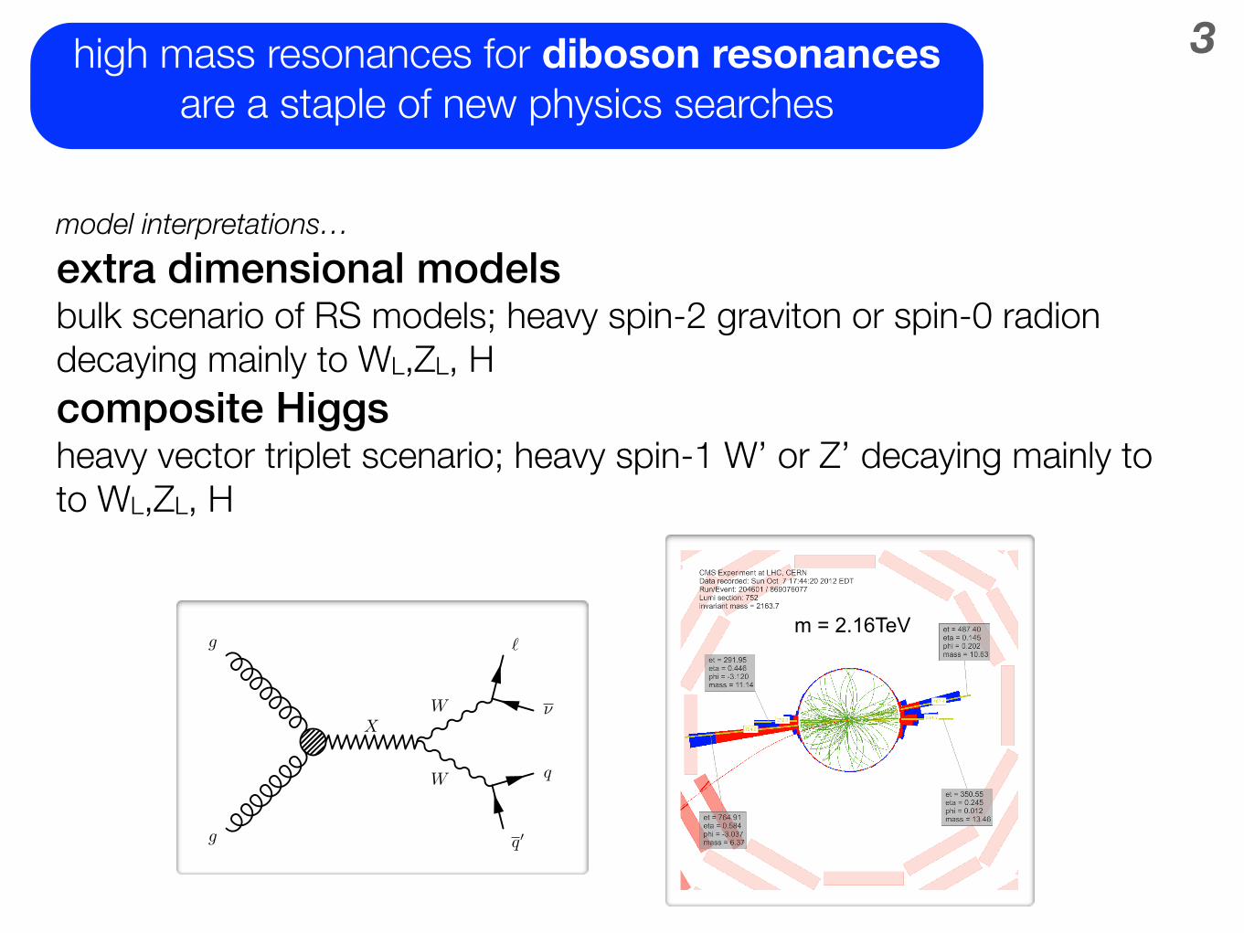
3high mass resonances for diboson resonances are a staple of new physics searches

Outline of the talk

2 11 Aug 2015 Andreas Hinzmann

•  Di-boson resonance models

•  Final state overview

•  WW/WZ/ZZ resonance searches

•  WH/ZH resonance searches

•  HH resonance searches

X

W

W

g

g

q0

q

⌫

`

g

gX

H

Hp

p

b

b

b

b

•model interpretations… •extra dimensional models •bulk scenario of RS models; heavy spin-2 graviton or spin-0 radion decaying mainly to WL,ZL, H

•composite Higgs •heavy vector triplet scenario; heavy spin-1 W’ or Z’ decaying mainly to to WL,ZL, H Final states with boosted W/Z/H


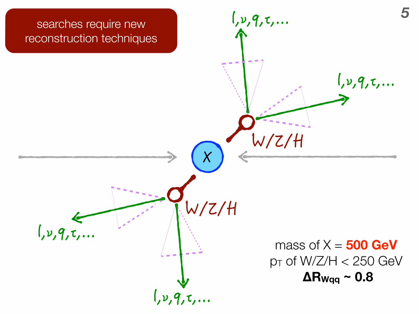
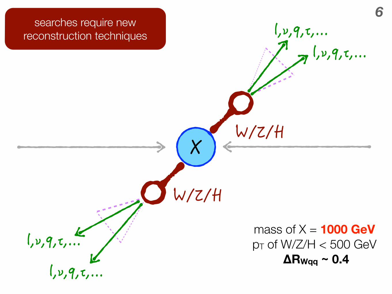
•  Above W,Z(H) pT>200(300) GeV quarks merge into R=0.8 jet •  Discrimination based on jet substructure in Run 1 di-boson analyses

•  Reconstruct W/Z/H with CA R=0.8 jet •  Pruned jet mass ! expected at W/Z/H mass •  N-subjettiness τ2/τ1 ! Should look like composed of two smaller jets •  Calibrated in semileptonic ttbar sample containing real boosted Ws

X

W

W

g

g

q0

q

⌫

`

quark

anti-quark m = 2.16TeV

ΔRqqmin ≈ Δθqq

min ≈ 2 MV

pT ,V

Details in backup

4

W Z H

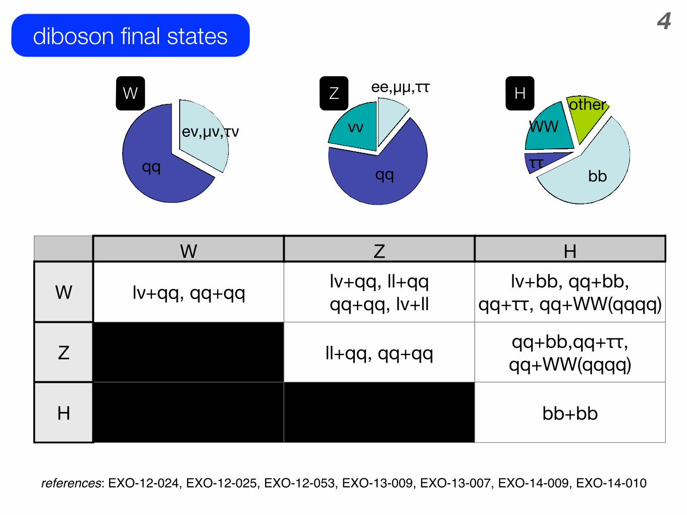
W lν+qq, qq+qq lv+qq, ll+qqqq+qq, lv+ll

lv+bb, qq+bb,qq+ττ, qq+WW(qqqq)

Z ll+qq, qq+qq qq+bb,qq+ττ, qq+WW(qqqq)

H bb+bb

diboson final states

qq

eν,μν,τν νν

qq

ee,μμ,ττother

WW

ττbb

ZW H

references: EXO-12-024, EXO-12-025, EXO-12-053, EXO-13-009, EXO-13-007, EXO-14-009, EXO-14-010

5

April

25, 2

014

�27

April 25, 2014�27

April 25, 2014�27

mass of X = 500 GeV pT of W/Z/H < 250 GeV

ΔRWqq ~ 0.8

searches require new reconstruction techniques

6

April

25, 2

014

�27

April 25, 2014

�27

mass of X = 1000 GeV pT of W/Z/H < 500 GeV

ΔRWqq ~ 0.4

searches require new reconstruction techniques

7merged W/Z qq

W or Z jet q/g jet

21τ-subjettiness ratio N

0 0.2 0.4 0.6 0.8 1

Even

ts / 0

.05

0

0.5

1

1.5

2

2.5

610×

Untagged data

MADGRAPH+PYTHIA

HERWIG++

2.94E+07) (JHUGEN+PYTHIA) × ZZ (→ (1.5TeV) bulkG

1.52E+07) (JHUGEN+PYTHIA) × WW (→ (1.5TeV) bulkG

8.51E+04) PYTHIA× WZ (→W’ (1.5 TeV)

1.34E+05) HERWIG++× ZZ (→ (1.5 TeV) RSG

7.15E+04) HERWIG++× WW (→ (1.5 TeV) RSG

= 8 TeVs, -1CMS, L = 19.7 fb

CA R=0.8

Pruned-jet mass (GeV)

0 50 100 150 200

Even

ts / 5

GeV

0

0.5

1

1.5

2

2.5

3

610×

Untagged data

MADGRAPH+PYTHIA

HERWIG++

2.94E+07) (JHUGEN+PYTHIA) × ZZ (→ (1.5TeV) bulkG

1.52E+07) (JHUGEN+PYTHIA) × WW (→ (1.5TeV) bulkG

8.51E+04) PYTHIA× WZ (→W’ (1.5 TeV)

1.34E+05) HERWIG++× ZZ (→ (1.5 TeV) RSG

7.15E+04) HERWIG++× WW (→ (1.5 TeV) RSG

= 8 TeVs, -1CMS, L = 19.7 fb

CA pruned R=0.8

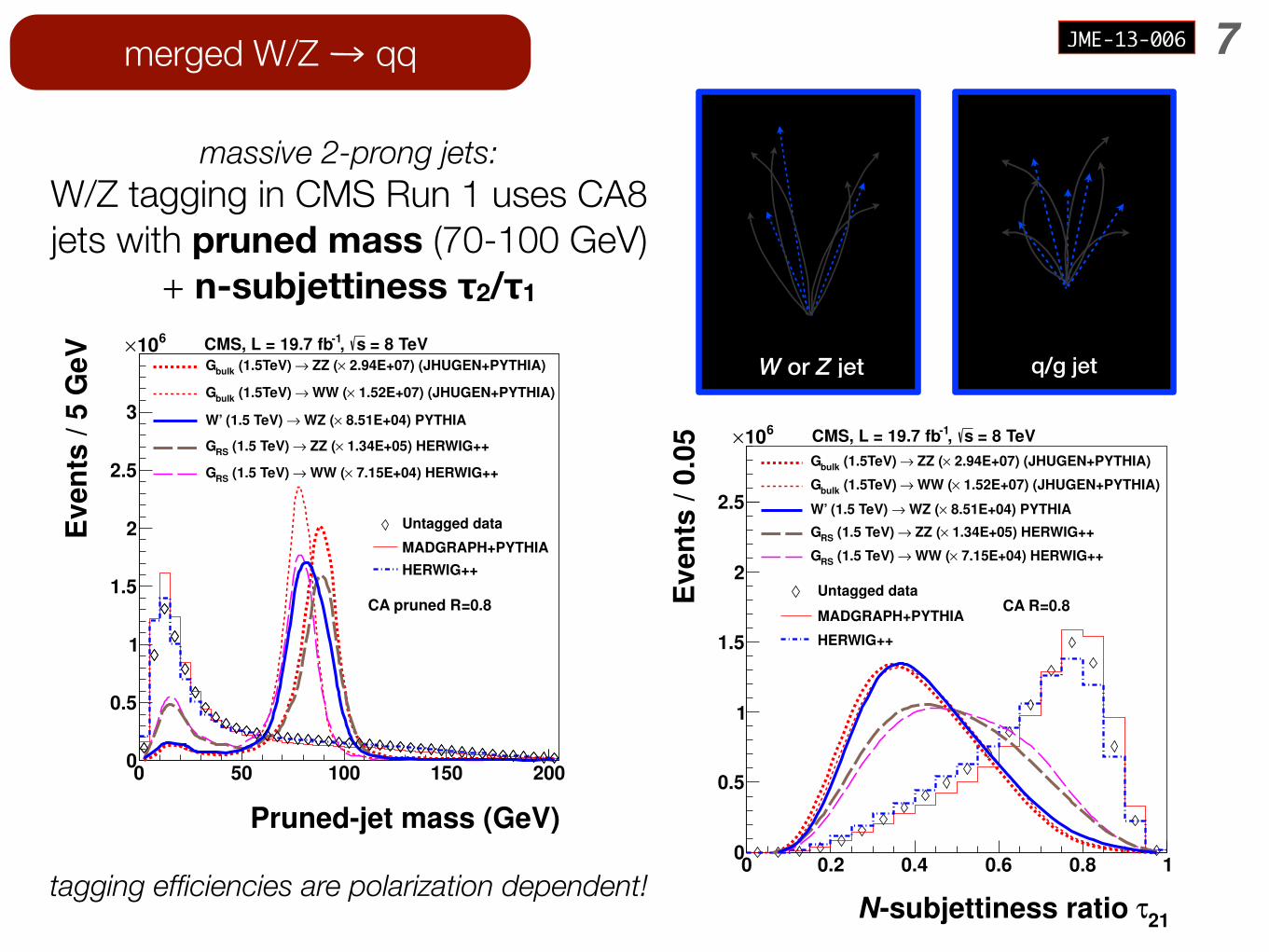
massive 2-prong jets: W/Z tagging in CMS Run 1 uses CA8 jets with pruned mass (70-100 GeV)

+ n-subjettiness τ2/τ1

JME-13-006

tagging efficiencies are polarization dependent!

8merged Z/H bb

Higgs jet

(GeV)jJet mass m0 50 100 150 200

Arbi

trary

sca

le

0

0.1

0.2

0.3

0.4q/g MADGRAPH+PYTHIA

q'bq → Wb →t b b→H

4q→ WW* →H q'q →W q q→Z

CA pruned R=0.8

CMSSimulation

8 TeV

[GeV/c]T

Fat jet p0 100 200 300 400 500 600 700 800 900 1000

Tagg

ing

effic

ienc

y

-210

-110

1

bb→H splittingbb→g

Hadronic ZHadronic topHadronic Wudsg jets

, Subjet IVFCSVL2<135 GeV/cpruned75<mAK R=0.8

(8 TeV)CMS Simulation Preliminary

8merged Z/H bb

15

Tagging Performance

Higgs channel

Top channel

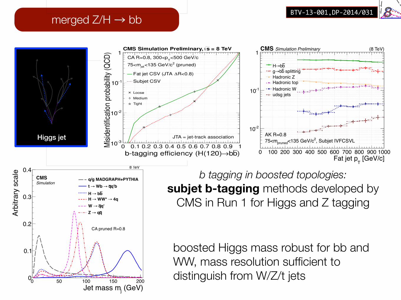
QCD mistag rate reduced up to a factor 10 with minor loss of efficiency

Higgs-tagging =double b-tagging +75 <m

jet< 135 GeV

double b-tagging Higgs tagging

tagging efficiency mistag rate

14

B-Tagging Performance

Higgs channel

Top channel

Overall subjet b-tagging performs better

medium boost regime large boost regime

Subjet b-tagging performs better

Fat-jet b-tagging suitable at very high p

T

Higgs jet

(GeV)jJet mass m0 50 100 150 200

Arbi

trary

sca

le

0

0.1

0.2

0.3

0.4q/g MADGRAPH+PYTHIA

q'bq → Wb →t b b→H

4q→ WW* →H q'q →W q q→Z

CA pruned R=0.8

CMSSimulation

8 TeV

b tagging in boosted topologies: subjet b-tagging methods developed by

CMS in Run 1 for Higgs and Z tagging

boosted Higgs mass robust for bb and WW, mass resolution sufficient to distinguish from W/Z/t jets

BTV-13-001,DP-2014/031

Even

ts

0

50

100

150

200

250 Data W - Data W +

MC W - MC W +

νµ → = 8 TeV, W s at -1CMS Preliminary, 19.3 fb

= 1.0)κjet charge (-0.8 -0.6 -0.4 -0.2 0 0.2 0.4 0.6 0.8

Dat

a / S

im

0.51

1.52

9merged H WW qqqqW/Z discrimination

42τ-subjettiness ratio N0 0.2 0.4 0.6 0.8 1

Acc

× X

X)

→(H

Β ×

42τddN

0

0.5

1

1.5

2

2.5

3

3.5

4-310×

b b→H 4q→ WW* →H

c c→H gg→H

ττ →H

< 135 GeVj110 < m

CMSSimulation

8 TeV

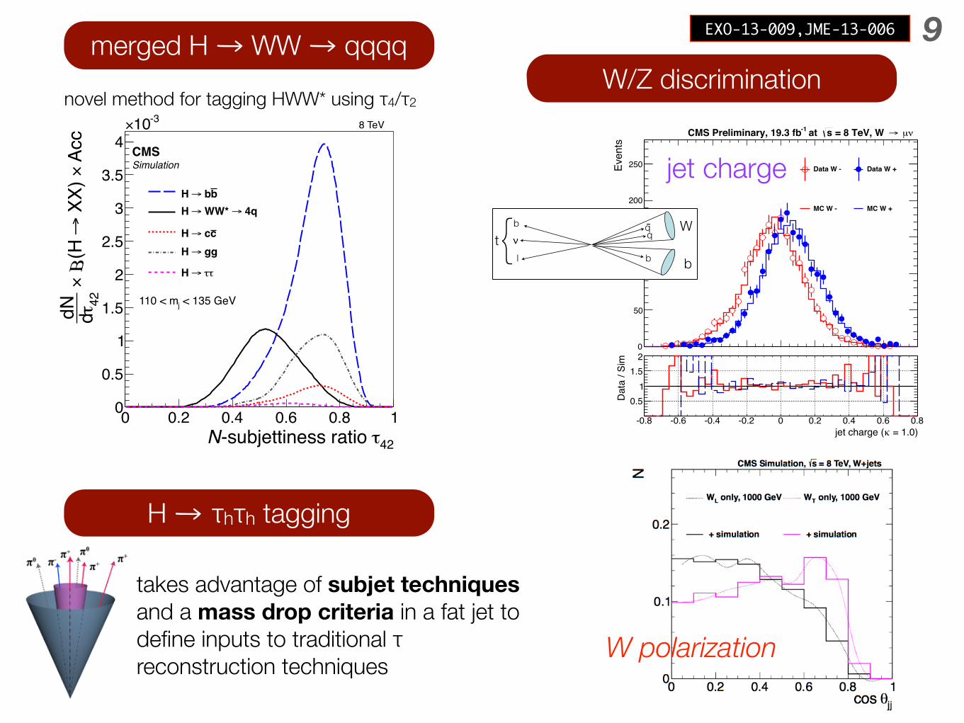
novel method for tagging HWW* using τ4/τ2

νb q

q-

blt

W

b{

W polarization

jet charge

EXO-13-009,JME-13-006

H τhτh tagging

takes advantage of subjet techniques and a mass drop criteria in a fat jet to define inputs to traditional τ reconstruction techniques

H!ττ-tagging


•  Main discriminator of taus against q/g-jets is isolation summing reconstructed particle energies in cone around tau decay products •  Decay products of one excluded from isolation

cone of other tau forming the H!ττ •  Higgs mass reconstructed from visible tau decay

products and missing transverse energy

[GeV]ττm0 50 100 150 200 250

[1/G

eV]

ττ1/

dm

0

0.02

0.04

0.06

0.08

0.1

0.12

0.14

0.16 = 125 GeVH mττ →H

ττ →Z

= 8 TeVsCMS Simulation hτµ

H

Z

10validation of QCD

νb q

q-

blt

W

b{

standard candles

Even

ts

0

1

2

3

4

5

6

310×

Data Z+Jets

Single Top WW/WZ/ZZ

W+jets Pythia W+jets Herwig

powhegtt MC Stat + Sys

= 8 TeV, W+jetss at -1CMS Preliminary, 19.3 fb

CA R = 0.8 < 350 GeV

T250 < p

|<2.4η|

1τ/2τ0.1 0.2 0.3 0.4 0.5 0.6 0.7 0.8 0.9 1

Dat

a / S

im

0.5

1

1.5

2

ν

lW{ q/gq/g q/g

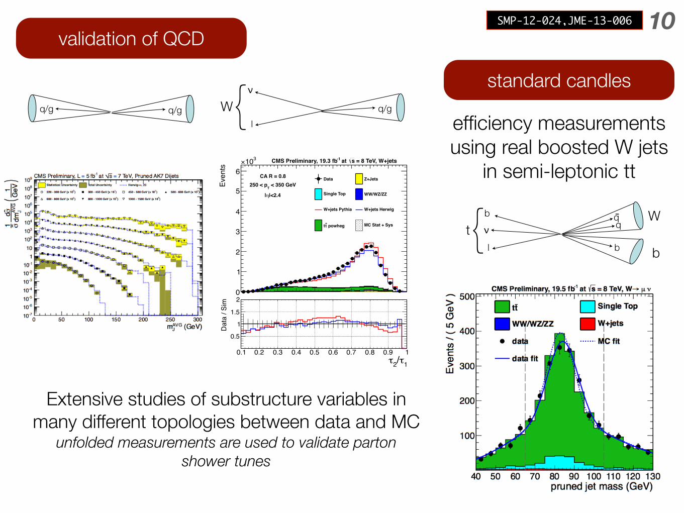
Extensive studies of substructure variables in many different topologies between data and MC

unfolded measurements are used to validate parton shower tunes

efficiency measurements using real boosted W jets

in semi-leptonic tt

SMP-12-024,JME-13-006

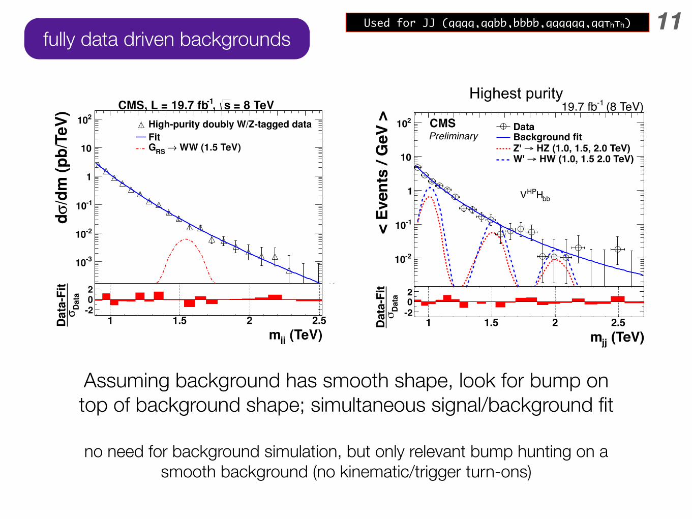
11fully data driven backgrounds

Background estimation – all-jets final states


•  Assumption: Background has a smooth distribution and can be described by a fit function

•  Simultaneously fit signal yield and background parameters

•  Advantages:

•  No need for background simulation •  Disadvantages:

•  Arbitrary choice of background functional form and a systematic uncertainty assigned to it

•  Not possible in regions of discontinuity due to trigger turn-ons or kinematic selections

•  Only works for bumps, not for enhancements in tails

•  Checks: •  Bias-test: How much is signal yield mis-fitted when fitting toy spectra of

default fit function with alternative functional form •  F-test: Increase number of parameters until fit shows no significant

improvement

310×

/dm

(p

b/T

eV

)σ

d

-310

-210

-110

1

10

210 High-purity doubly W/Z-tagged data

Fit WW (1.5 TeV)→ RSG

= 8 TeVs, -1CMS, L = 19.7 fb

(TeV)jjm1 1.5 2 2.5

Da

taσ

Da

ta-F

it

-202

V(qq)H(bb) resonances


•  Same search techniques as V(qq)V(qq) search •  Lower backgrounds due to better background rejection of H(bb)-tagger

compared to W(qq)/Z(qq)-tagger

Dijet Mass (GeV)1 1.2 1.4 1.6 1.8 2 2.2 2.4 2.6

< Ev

ents

/ G

eV >

-310

-210

-110

1

10

210 DataBackground fit

HZ (1.0, 1.5, 2.0 TeV)→Z' HW (1.0, 1.5 2.0 TeV)→W'

bbHHPV

(8 TeV)-119.7 fbCMSPreliminary

(TeV)jjm1 1.5 2 2.5

Dat

aσ

Dat

a-Fi

t

-202

arXiv:1506.01443

Dijet Mass (GeV)1 1.2 1.4 1.6 1.8 2 2.2 2.4 2.6

< Ev

ents

/ G

eV >

-310

-210

-110

1

10


HZ (1.0, 1.5, 2.0 TeV)→Z' HW (1.0, 1.5 2.0 TeV)→W'

bbHLPV


(TeV)jjm1 1.5 2 2.5

Dat

aσ

Dat

a-Fi

t

-202

Highest purity Lower purity

Assuming background has smooth shape, look for bump on top of background shape; simultaneous signal/background fit

no need for background simulation, but only relevant bump hunting on a smooth background (no kinematic/trigger turn-ons)

Used for JJ (qqqq,qqbb,bbbb,qqqqqq,qqτhτh)

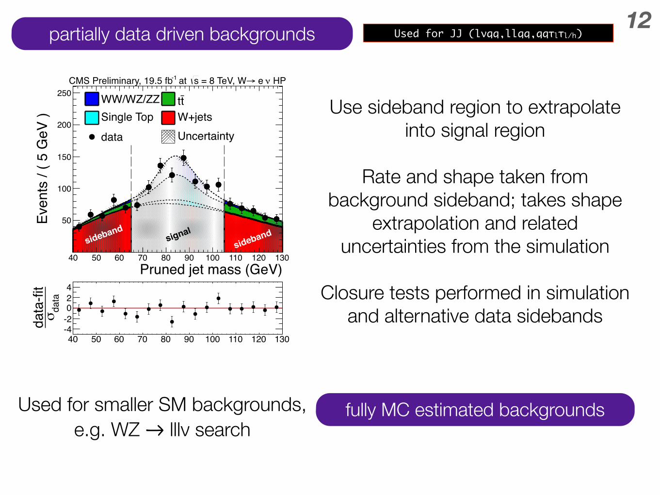
12partially data driven backgrounds

fully MC estimated backgrounds

Use sideband region to extrapolate into signal region

Rate and shape taken from background sideband; takes shape

extrapolation and related uncertainties from the simulation

Closure tests performed in simulation and alternative data sidebands

(GeV)WWm1000 1500 2000 2500 3000

arbi

trary

uni

t

0

0.05

0.1

0.15

0.2

0.25 SidebandSignal Regionα

: Alternate PSα: Alternate Functionα

σ 1± ασ 2± α α

0

1

2

3

4

5

6

7

HPν e → = 8 TeV, Ws at -1CMS Preliminary, 19.5 fb

Background – leptons+jets final states


•  Assumption: Observable in signal-depleted sideband closely related to signal region

•  Background rate+shape estimated from data in sideband extrapolated to signal region using simulation

•  Advantages: •  Limited use of background simulation •  Can search for enhancements in tails,

not only bumps

•  Disadvantages: •  Uncertainties associated to extrapolation

to signal region sometimes arbitrary

•  Checks: •  Closure test in simulation and/or other

data sideband

arXiv:1405.3447

40 50 60 70 80 90 100 110 120 130

data

σdata

-fit

-4-2024

Pruned jet mass (GeV)40 50 60 70 80 90 100 110 120 130

Even

ts /

( 5 G

eV )

50

100

150

200

250 WW/WZ/ZZ ttSingle Top W+jetsdata Uncertainty

HPν e → = 8 TeV, Ws at -1CMS Preliminary, 19.5 fb

Used for smaller SM backgrounds, e.g. WZ lllν search

Used for JJ (lνqq,llqq,qqτlτl/h)

sidebandsidebandsignal

13

results

V V V H H H

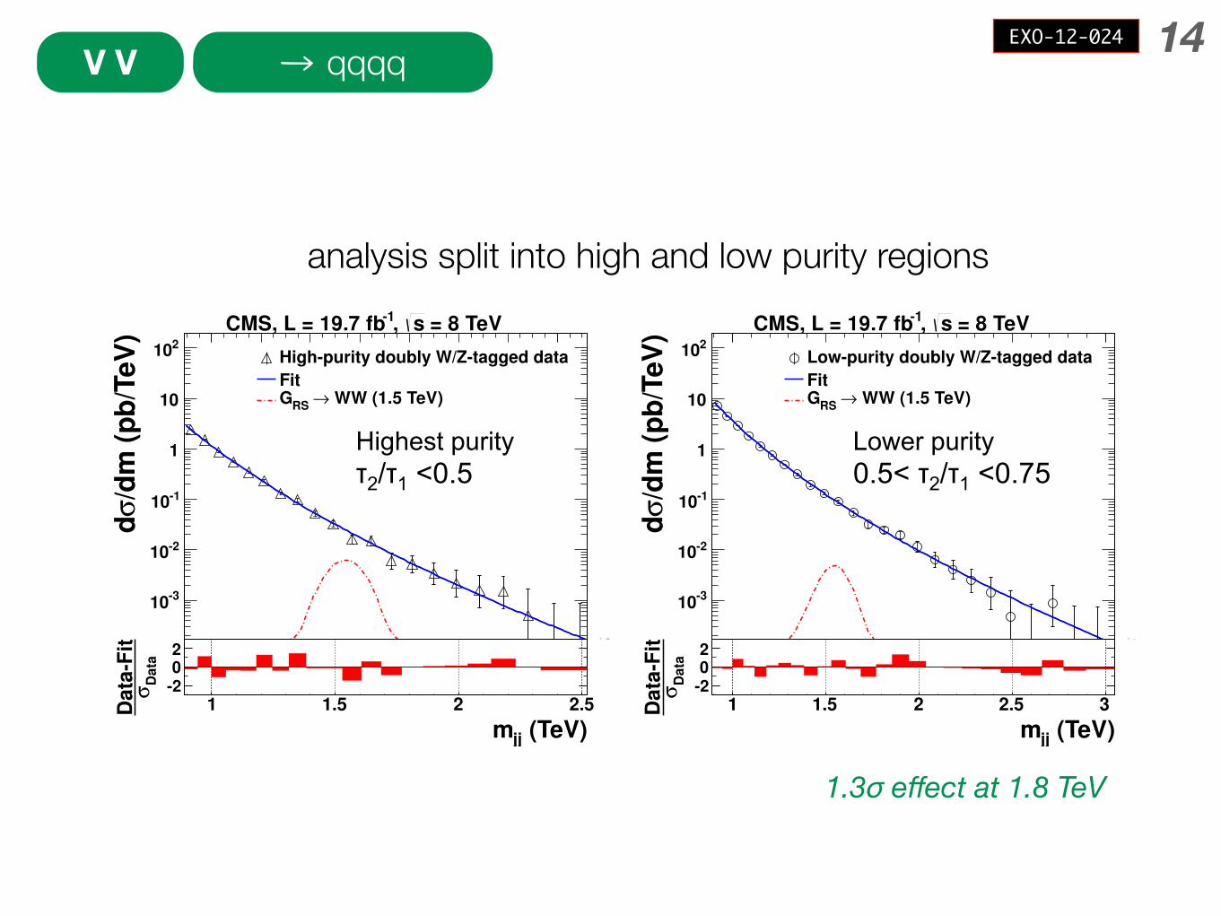
14qqqq

•  ATLAS sees excess at 2 TeV with 2.5 s.d. global signficance (arXiv:1506.00962)

•  CMS higher+lower purity combined signficance at 1.8 TeV is 1.3 s.d.

310×

/dm

(p

b/T

eV

)σ

d

-310

-210

-110

1

10

210 Low-purity doubly W/Z-tagged data


= 8 TeVs, -1CMS, L = 19.7 fb

(TeV)jjm1 1.5 2 2.5 3

Da

taσ

Data

-Fit

-202

310×

/dm

(p

b/T

eV

)σ

d

-310

-210

-110

1

10

210 High-purity doubly W/Z-tagged data


= 8 TeVs, -1CMS, L = 19.7 fb

(TeV)jjm1 1.5 2 2.5

Da

taσ

Data

-Fit

-202

V(qq)V(qq) resonances in dijets – 2


Highest purity τ2/τ1 <0.5

Lower purity 0.5< τ2/τ1 <0.75

arXiv:1405.1994 1.3σ effect at 1.8 TeV

V V

analysis split into high and low purity regions

EXO-12-024

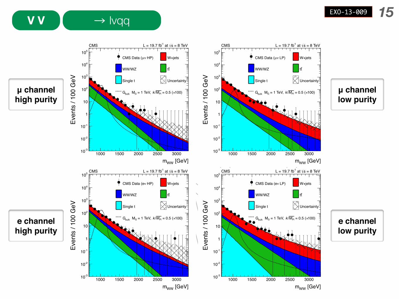
15lνqqV V

14 6 Modeling of background and signal

[GeV]WWm1000 1500 2000 2500 3000

Even

ts /

100

GeV

-310

-210

-110

1

10

210

310

410

510 HP)νµCMS Data ( W+jets

WW/WZ tt

Single t Uncertainty

100)× = 0.5 (PlM/k = 1 TeV, G MbulkG

= 8 TeVs at -1CMS L = 19.7 fb

[GeV]WWm1000 1500 2000 2500 3000

Even

ts /

100

GeV

-310

-210

-110

1

10

210

310

410

510 LP)νµCMS Data ( W+jets

WW/WZ tt


100)× = 0.5 (PlM/k = 1 TeV, G MbulkG


[GeV]WWm1000 1500 2000 2500 3000

Even

ts /

100

GeV

-310

-210

-110

1

10

210

310

410

510

HP)νCMS Data (e W+jets

WW/WZ tt


100)× = 0.5 (PlM/k = 1 TeV, G MbulkG


[GeV]WWm1000 1500 2000 2500 3000

Even

ts /

100

GeV

-310

-210

-110

1

10

210

310

410

510

LP)νCMS Data (e W+jets

WW/WZ tt


100)× = 0.5 (PlM/k = 1 TeV, G MbulkG


Figure 7: Final distributions in mWW for data and expected backgrounds for both the muon(top) and the electron (bottom) channels, high-purity (left) and low-purity (right) categories.The 68% error bars for Poisson event counts are obtained from the Neyman construction asdescribed in Ref. [75]. Also shown is a hypothetical bulk graviton signal with mass of 1000 GeVand k/MPl = 0.5. The normalization of the signal distribution is scaled up by a factor of 100for a better visualization.

e channelhigh purity

e channellow purity

μ channellow purity

μ channelhigh purity

EXO-13-009

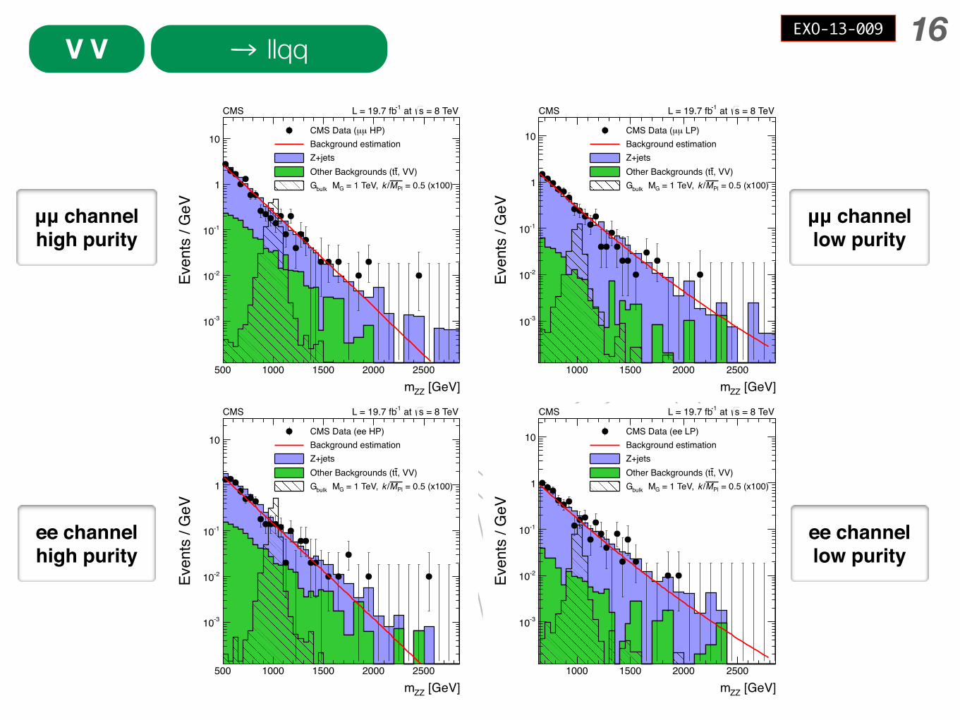
16llqqV V

6.1 Background estimation 15

[GeV]ZZm500 1000 1500 2000 2500

Even

ts /

GeV

-310

-210

-110

1

10 HP)µµCMS Data (

Background estimationZ+jets

, VV)tOther Backgrounds (t = 0.5 (x100)PlM/k = 1 TeV, G MbulkG


[GeV]ZZm1000 1500 2000 2500

Even

ts /

GeV

-310

-210

-110

1

10 LP)µµCMS Data (Background estimationZ+jets



[GeV]ZZm500 1000 1500 2000 2500

Even

ts /

GeV

-310

-210

-110

1

10CMS Data (ee HP)Background estimationZ+jets



[GeV]ZZm1000 1500 2000 2500

Even

ts /

GeV

-310

-210

-110

1

10 CMS Data (ee LP)Background estimationZ+jets



Figure 8: Final distributions in mZZ for data and expected backgrounds for both the muon (top)and the electron (bottom) channels, high-purity (left) and low-purity (right) categories. Pointswith error bars show distributions of data; solid histograms depict the different componentsof the background expectation from simulated events. The 68% error bars for Poisson eventcounts are obtained from the Neyman construction as described in Ref. [75]. Also shown is ahypothetical bulk graviton signal with mass of 1000 GeV and k/MPl = 0.5. The normalizationof the signal distribution is scaled up by a factor of 100 for a better visualization. The solid lineshows the central value of the background predicted from the sideband extrapolation proce-dure.

ee channelhigh purity

ee channellow purity

μμ channellow purity

μμ channelhigh purity

EXO-13-009

17

[GeV]GM1000 1500 2000 2500

) [pb

]bu

lk G

→ (p

p 95

%σ

-310

-210

-110

1 observedS

Frequentist CL

σ 1± expected S

Frequentist CL

σ 2± expected S

Frequentist CL

= 0.5PlM/k), bulk G→ (pp THσ

I II III

CMS = 8 TeVs at -1L = 19.7 fb

600

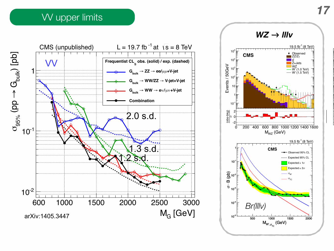
Limits on spin-2 WW/ZZ resonances


•  Run I searches start to be sensitive to gravitons in Bulk model •  Cross section and width related to coupling parameter k/Mpl

•  Narrow width for k/Mpl ≤ 0.5 •  Model independent limits provided allowing reinterpretation for wide width

resonance and as spin-1 WZ resonance (see later)

VV

k/Mpl=0.5

k/Mpl=1.0

[GeV]GM1000 1500 2000 2500 3000

) [pb

]bu

lk G

→ (p

p 95

%σ

-210

-110

1

CMS (unpublished) = 8 TeVs at -1L = 19.7 fb

600

obs. (solid) / exp. (dashed)S

Frequentist CL

+V-jetµµ ee/→ ZZ → bulkG

V-jet+V-jet→ WW/ZZ → bulkG

+V-jetνµ/ν e→ WW → bulkG

Combination

VV

arXiv:1405.3447

1.2 s.d.

2.0 s.d.

1.3 s.d.

VV upper limits

6 5 Systematic uncertainties

optimal values are then plotted as a function of the WZ mass and an analytic function is fit to229

the resulting distribution. For the mass-window requirement, two regimes of linear behavior230

are observed: for masses less than 1200 GeV, a narrow mass window is optimal in order to231

reject as much background as possible. Above 1200 GeV, the background ceases to contribute232

significantly and it is better to have a large mass window. The LT requirement exhibits a linear233

relationship: as the mass increases, it is optimal to require a larger LT, until around 1000 GeV,234

at which point having LT greater than 500 GeV is sufficient. These mass windows and LT re-235

quirements are summarized in Table 1.236

0 200 400 600 800 1000 1200 1400 1600

Even

ts /

50G

eV

-110

1

10

210

310

410

510CMS

(8 TeV)-119.5 fb

ObservedγZZ/Z

ttZ+JetsWZW' (1.0 TeV)W' (1.5 TeV)

(GeV)WZM0 200 400 600 800 1000 1200 1400 1600

σ(o

bs-b

kg)

-202 0 100 200 300 400 500 600 700 800

Even

ts /

100

GeV

-110

1

10

210

310

410

510CMS

(8 TeV)-119.5 fb

ObservedγZZ/Z

ttZ+JetsWZW' (1.0 TeV)W' (1.5 TeV)

(GeV)lT

pΣ ≡ TL0 100 200 300 400 500 600 700 800

σ(o

bs-b

kg)

-202

Figure 1: The WZ invariant mass (left) and LT (right) distributions for the background, signal,and observed events after the WZ candidate selection. The last bin includes overflow events.The (obs � bkg)/s in the lower panel is defined as the difference between the number of ob-served events and the number of expected background events divided by the total statisticaluncertainty.

5 Systematic uncertainties237

Systematic uncertainties affecting the analysis can be grouped into four categories. In the first238

group we include uncertainties that are determined from simulation. These include uncertain-239

ties in the lepton and EmissT energy scales and resolution, as well as uncertainties in the PDFs.240

Following the recommendations of the PDF4LHC group [53, 54], PDF and as variations of the241

MSTW2008 [55], CT10 [56], and NNPDF2.0 [57] PDF sets are taken into account and their im-242

pact on the WZ cross section estimated. Signal PDF uncertainties are taken into account only243

to derive uncertainty bands around the signal cross sections, as shown in Fig. 2, and do not244

impact the central limit. An uncertainty associated with the simulation of pileup is also taken245

into account.246

The second group includes the systematic uncertainties affecting the observed-to-simulated247

scale factors for the efficiencies of the trigger, reconstruction, and identification requirements.248

These efficiencies are derived from tag-and-probe studies, and the uncertainty in the ratio of249

the efficiencies is typically taken as the systematic uncertainty. For the Z ! ee channel, we250

assign a 2% uncertainty related to the trigger scale factors, another 2% to account for the dif-251

ference between the observed and simulated reconstruction efficiencies, and an additional 1%252

uncertainty related to the electron identification and isolation scale factors. For the Z ! µµ253

WZ lllν

10 7 Summary

(GeV)TCρW', M

500 1000 1500 2000

B (p

b)⋅

σ

-510

-410

-310

-210

-110

1

(GeV)TCρW', M

500 1000 1500 2000

B (p

b)⋅

σ

-510

-410

-310

-210

-110

1 CMS

(8 TeV)-119.5 fb

Observed 95% CL

Expected 95% CL

σ 1±Expected

σ 2±Expected

W'σ

TCσ

Figure 2: Limits at 95% CL on s ⇥B(W0 ! 3`n) as a function of the mass of the EGM W0 (blue)and rTC (red), along with the 1 s and 2 s combined statistical and systematic uncertainties in-dicated by the green (dark) and yellow (light) band, respectively. The theoretical cross sectionsinclude a mass-dependent NNLO K-factor. The thickness of the theory lines represents thePDF uncertainty associated with the signal cross sections. The predicted cross sections for rTCassume that MpTC = 3

4 MrTC � 25 GeV and that the LSTC parameter sin c = 1/3.

Acknowledgments316

We congratulate our colleagues in the CERN accelerator departments for the excellent perfor-317

mance of the LHC and thank the technical and administrative staffs at CERN and at other CMS318

institutes for their contributions to the success of the CMS effort. In addition, we gratefully319

acknowledge the computing centres and personnel of the Worldwide LHC Computing Grid320

for delivering so effectively the computing infrastructure essential to our analyses. Finally, we321

acknowledge the enduring support for the construction and operation of the LHC and the CMS322

detector provided by the following funding agencies: BMWFW and FWF (Austria); FNRS and323

FWO (Belgium); CNPq, CAPES, FAPERJ, and FAPESP (Brazil); MES (Bulgaria); CERN; CAS,324

MoST, and NSFC (China); COLCIENCIAS (Colombia); MSES and CSF (Croatia); RPF (Cyprus);325

MoER, ERC IUT and ERDF (Estonia); Academy of Finland, MEC, and HIP (Finland); CEA and326

CNRS/IN2P3 (France); BMBF, DFG, and HGF (Germany); GSRT (Greece); OTKA and NIH327

(Hungary); DAE and DST (India); IPM (Iran); SFI (Ireland); INFN (Italy); NRF and WCU (Re-328

public of Korea); LAS (Lithuania); MOE and UM (Malaysia); CINVESTAV, CONACYT, SEP,329

and UASLP-FAI (Mexico); MBIE (New Zealand); PAEC (Pakistan); MSHE and NSC (Poland);330

FCT (Portugal); JINR (Dubna); MON, RosAtom, RAS and RFBR (Russia); MESTD (Serbia);331

SEIDI and CPAN (Spain); Swiss Funding Agencies (Switzerland); MST (Taipei); ThEPCenter,332

IPST, STAR and NSTDA (Thailand); TUBITAK and TAEK (Turkey); NASU and SFFR (Ukraine);333

STFC (United Kingdom); DOE and NSF (USA).334

Individuals have received support from the Marie-Curie programme and the European Re-335

search Council and EPLANET (European Union); the Leventis Foundation; the A. P. Sloan336

Foundation; the Alexander von Humboldt Foundation; the Belgian Federal Science Policy Of-337

fice; the Fonds pour la Formation a la Recherche dans l’Industrie et dans l’Agriculture (FRIA-338

Br(lllν)

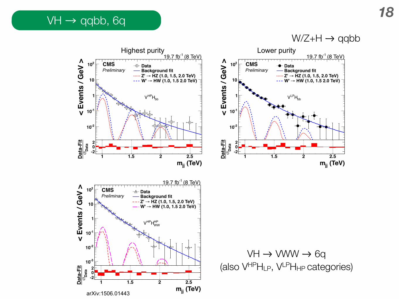
18VH qqbb, 6q

V(qq)H(bb) resonances


•  Same search techniques as V(qq)V(qq) search •  Lower backgrounds due to better background rejection of H(bb)-tagger

compared to W(qq)/Z(qq)-tagger

Dijet Mass (GeV)1 1.2 1.4 1.6 1.8 2 2.2 2.4 2.6

< Ev

ents

/ G

eV >

-310

-210

-110

1

10


HZ (1.0, 1.5, 2.0 TeV)→Z' HW (1.0, 1.5 2.0 TeV)→W'

bbHHPV


(TeV)jjm1 1.5 2 2.5

Dat

aσ

Dat

a-Fi

t

-202

arXiv:1506.01443

Dijet Mass (GeV)1 1.2 1.4 1.6 1.8 2 2.2 2.4 2.6

< Ev

ents

/ G

eV >

-310

-210

-110

1

10


HZ (1.0, 1.5, 2.0 TeV)→Z' HW (1.0, 1.5 2.0 TeV)→W'

bbHLPV


(TeV)jjm1 1.5 2 2.5

Dat

aσ

Dat

a-Fi

t

-202

Highest purity Lower purity

V(qq)H(WW!qqqq) resonances


•  Exclusive search channel: Only events that fail H(bb) tagger

•  Factor 4 less stringent limits on cross section than H(bb) channel •  Still adds 10% to combination with H(bb)

•  For Run II also consider H(WW!lvqq) jets

Dijet Mass (GeV)1 1.2 1.4 1.6 1.8 2 2.2 2.4 2.6

< Ev

ents

/ G

eV >

-310

-210

-110

1

10


HZ (1.0, 1.5, 2.0 TeV)→Z' HW (1.0, 1.5 2.0 TeV)→W'

HPWWHHPV


(TeV)jjm1 1.5 2 2.5

Dat

aσ

Dat

a-Fi

t

-202

arXiv:1506.01443

VH VWW 6q (also VHPHLP, VLPHHP categories)

W/Z+H qqbb

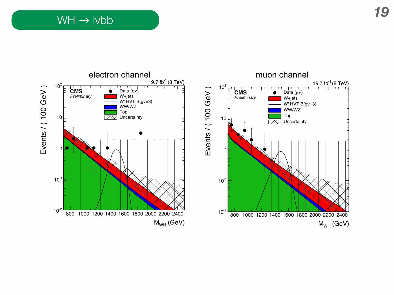
19WH lνbb

W(lv)H(bb) resonances


•  Same search techniques as W(lv)V(qq) search •  Lower backgrounds due to better background rejection of H(bb)-tagger

compared to W(qq)/Z(qq)-tagger •  Excess in W(lv)H(bb) at 1.8 TeV has a global significance of 2.2 s.d.

(GeV)WHM800 1000 1200 1400 1600 1800 2000 2200 2400

Even

ts /

( 100

GeV

)

-210

-110

1

10

210)νData (e

W+jetsW' HVT B(gv=3)WW/WZTopUncertainty

(8 TeV)-119.7 fb

CMSPreliminary

(GeV)WHM800 1000 1200 1400 1600 1800 2000 2200 2400

Even

ts /

( 100

GeV

)-210

-110

1

10

210)νµData (

W+jetsW' HVT B(gv=3)WW/WZTopUncertainty

(8 TeV)-119.7 fb

CMSPreliminary

CMS-PAS-EXO-14-010

muon channel electron channel

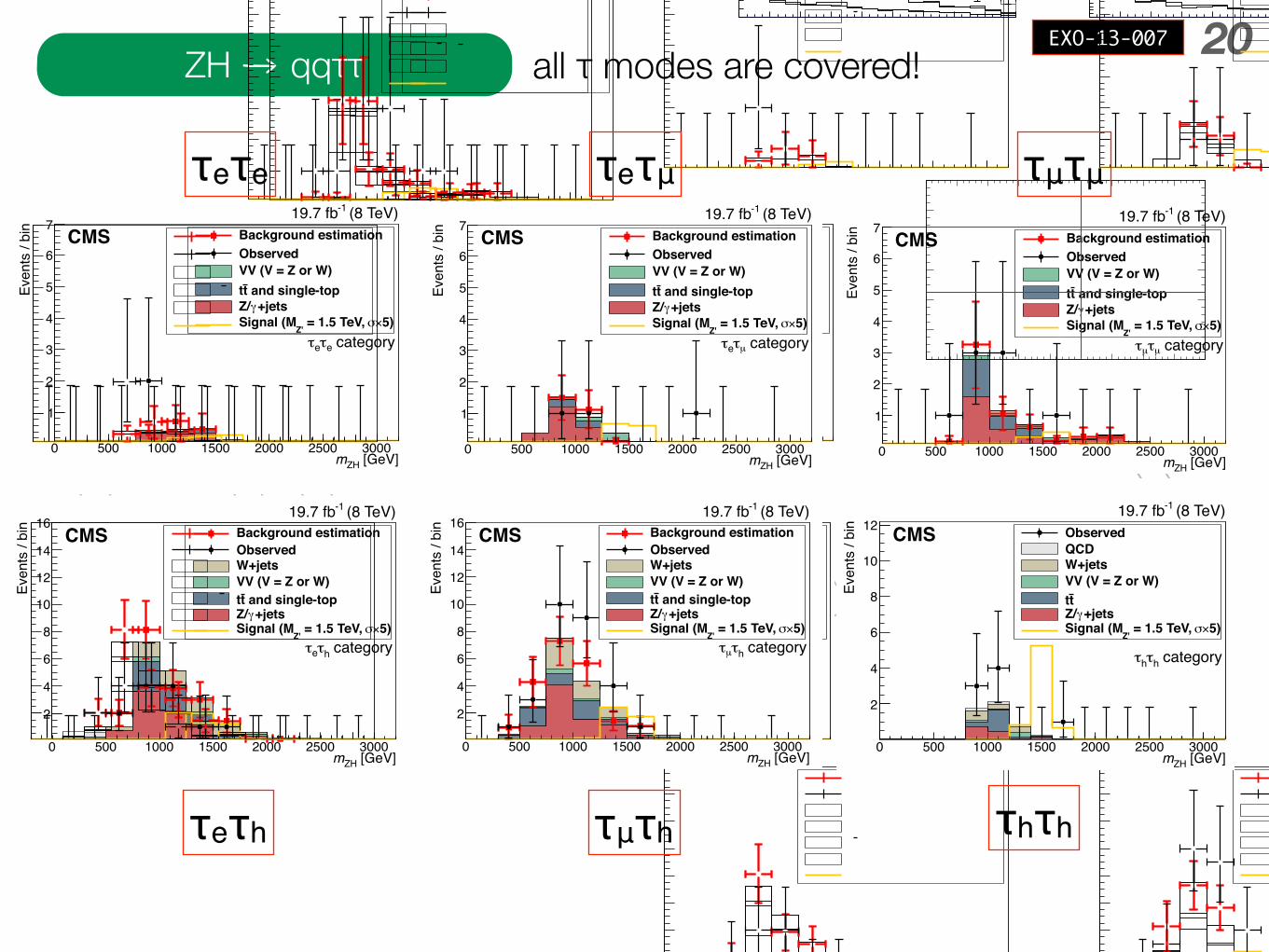
20ZH qqττ all τ modes are covered!EXO-13-007


[GeV]ZHm0 500 1000 1500 2000 2500 3000

Even

ts /

bin

1

2

3

4

5

6

7Background estimationObservedVV (V = Z or W)

and single-toptt+jetsγZ/

5)×σ = 1.5 TeV, Z'Signal (M

(8 TeV)-119.7 fbCMS

categoryeτeτ

[GeV]ZHm0 500 1000 1500 2000 2500 3000

Even

ts /

bin

1

2

3

4

5

6




(8 TeV)-119.7 fbCMS

categoryµτeτ

[GeV]ZHm0 500 1000 1500 2000 2500 3000

Even

ts /

bin

1

2

3

4

5

6




(8 TeV)-119.7 fbCMS

categoryµτµτ

Figure 1: Observed distributions of mZH for the all-leptonic channels along with the corre-sponding MC expectations for signal and background, as well as background estimation de-rived from data: (top left) tete category; (top right) tetµ category; (bottom) tµtµ category. Tenequal-size histogram bins cover the region from 0 to 2.5 TeV, while a single bin is used at highermZH because of the limited number of MC and data events. The signal cross section is scaledby a factor of 5.

[GeV]ZHm0 500 1000 1500 2000 2500 3000

Even

ts /

bin

2

4

6

8

10

12

14

16 Background estimationObservedW+jetsVV (V = Z or W)



(8 TeV)-119.7 fbCMS

categoryhτeτ

[GeV]ZHm0 500 1000 1500 2000 2500 3000

Even

ts /

bin

2

4

6

8

10

12

14




(8 TeV)-119.7 fbCMS

categoryhτµτ

Figure 2: Observed distributions of mZH for the semileptonic channels along with the corre-sponding MC expectations for signal and background, as well as background estimation de-rived from data: (left) teth category; (right) tµth category. Ten equal-size histogram bins coverthe region from 0 to 2.5 TeV, while a single bin is used at higher mZH because of the limitednumber of MC and data events. The signal cross section is scaled by a factor of 5.


[GeV]ZHm0 500 1000 1500 2000 2500 3000

Even

ts /

bin

1

2

3

4

5

6




(8 TeV)-119.7 fbCMS

categoryeτeτ

[GeV]ZHm0 500 1000 1500 2000 2500 3000

Even

ts /

bin

1

2

3

4

5

6




(8 TeV)-119.7 fbCMS

categoryµτeτ

[GeV]ZHm0 500 1000 1500 2000 2500 3000

Even

ts /

bin

1

2

3

4

5

6




(8 TeV)-119.7 fbCMS

categoryµτµτ


[GeV]ZHm0 500 1000 1500 2000 2500 3000

Even

ts /

bin

2

4

6

8

10

12

14




(8 TeV)-119.7 fbCMS

categoryhτeτ

[GeV]ZHm0 500 1000 1500 2000 2500 3000

Even

ts /

bin

2

4

6

8

10

12

14




(8 TeV)-119.7 fbCMS

categoryhτµτ



[GeV]ZHm0 500 1000 1500 2000 2500 3000

Even

ts /

bin

1

2

3

4

5

6




(8 TeV)-119.7 fbCMS

categoryeτeτ

[GeV]ZHm0 500 1000 1500 2000 2500 3000

Even

ts /

bin

1

2

3

4

5

6




(8 TeV)-119.7 fbCMS

categoryµτeτ

[GeV]ZHm0 500 1000 1500 2000 2500 3000

Even

ts /

bin

1

2

3

4

5

6




(8 TeV)-119.7 fbCMS

categoryµτµτ


[GeV]ZHm0 500 1000 1500 2000 2500 3000

Even

ts /

bin

2

4

6

8

10

12

14




(8 TeV)-119.7 fbCMS

categoryhτeτ

[GeV]ZHm0 500 1000 1500 2000 2500 3000

Even

ts /

bin

2

4

6

8

10

12

14




(8 TeV)-119.7 fbCMS

categoryhτµτ



[GeV]ZHm0 500 1000 1500 2000 2500 3000

Even

ts /

bin

1

2

3

4

5

6




(8 TeV)-119.7 fbCMS

categoryeτeτ

[GeV]ZHm0 500 1000 1500 2000 2500 3000

Even

ts /

bin

1

2

3

4

5

6




(8 TeV)-119.7 fbCMS

categoryµτeτ

[GeV]ZHm0 500 1000 1500 2000 2500 3000

Even

ts /

bin

1

2

3

4

5

6




(8 TeV)-119.7 fbCMS

categoryµτµτ


[GeV]ZHm0 500 1000 1500 2000 2500 3000

Even

ts /

bin

2

4

6

8

10

12

14




(8 TeV)-119.7 fbCMS

categoryhτeτ

[GeV]ZHm0 500 1000 1500 2000 2500 3000

Even

ts /

bin

2

4

6

8

10

12

14




(8 TeV)-119.7 fbCMS

categoryhτµτ



[GeV]ZHm0 500 1000 1500 2000 2500 3000

Even

ts /

bin

1

2

3

4

5

6




(8 TeV)-119.7 fbCMS

categoryeτeτ

[GeV]ZHm0 500 1000 1500 2000 2500 3000

Even

ts /

bin

1

2

3

4

5

6




(8 TeV)-119.7 fbCMS

categoryµτeτ

[GeV]ZHm0 500 1000 1500 2000 2500 3000

Even

ts /

bin

1

2

3

4

5

6




(8 TeV)-119.7 fbCMS

categoryµτµτ


[GeV]ZHm0 500 1000 1500 2000 2500 3000

Even

ts /

bin

2

4

6

8

10

12

14




(8 TeV)-119.7 fbCMS

categoryhτeτ

[GeV]ZHm0 500 1000 1500 2000 2500 3000

Even

ts /

bin

2

4

6

8

10

12

14




(8 TeV)-119.7 fbCMS

categoryhτµτ


9

[GeV]Pjetm

20 40 60 80 100 120 140 160 180 200

Even

ts /

10 G

eV

0

20

40

60

80

100 ObservedFit to ObservationFit to Simulation

and single-topttQCDW+jetsVV (V = Z or W)

+jetsγZ/

(8 TeV)-119.7 fbCMS

categoryhτeτ

[GeV]Pjetm

20 40 60 80 100 120 140 160 180 200

Even

ts /

10 G

eV

0102030405060708090 Observed

Fit to ObservationFit to Simulation

and single-topttQCDW+jetsVV (V = Z or W)

+jetsγZ/

(8 TeV)-119.7 fbCMS

categoryhτµτ

Figure 3: Observed distributions of mPjet for the semileptonic channels along with the corre-

sponding MC expectations for signal and background: (left) teth category; (right) tµth category.Fits are performed for MC and data (as discussed in the text).

[GeV]Pjetm

20 30 40 50 60 70 80 90 100 110

[GeV

]ττ

m

60

80

100

120

140

160

180

Figure 4: Definitions of the A, B, C, and D regions in the mPjet / mtt plane used in the background

estimation for the all-hadronic channel.

[GeV]ZHm0 500 1000 1500 2000 2500 3000

Even

ts /

bin

2

4

6

8

10

12 (8 TeV)-119.7 fb

CMS

categoryhτhτ

ObservedQCDW+jetsVV (V = Z or W)tt

+jetsγZ/5)×σ = 1.5 TeV, Z'Signal (M

Figure 5: Observed distributions of mZH for the thth category along with the correspondingMC expectations for signal and background. Ten equal-size histogram bins cover the regionfrom 0 to 2.5 TeV, while a single bin is used at higher mZH because of the limited number of MCand data events. The signal cross section is scaled by a factor of 5.

τeτe τeτμ τμτμ

τμτhτeτh τhτh

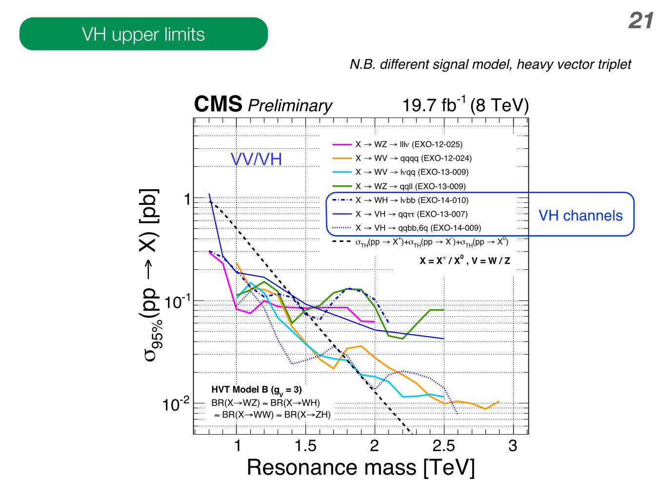
21•  Heavy Vector Triplet model B (composite Higgs-like model) m(W’)=m(Z’) excluded up to 1.8 TeV •  WV(lvqq), VV(qqqq) and VH(qqbb) have best sensitivity at high masses

Resonance mass [TeV]1 1.5 2 2.5 3

X) [

pb]

→(p

p 95

%σ

-210

-110

1

(EXO-12-025)ν lll→ WZ →X qqqq (EXO-12-024)→ WV →X

qq (EXO-13-009)ν l→ WV →X qqll (EXO-13-009)→ WZ →X

bb (EXO-14-010)ν l→ WH →X (EXO-13-007)ττ qq→ VH →X

qqbb,6q (EXO-14-009)→ VH →X )0 X→(pp THσ)+- X→(pp THσ)++ X→(pp THσ

= 3)V

HVT Model B (gWH)→ BR(X≈WZ) →BR(X

ZH)→ BR(X≈WW) → BR(X≈

, V = W / Z0 / X±X = X

(8 TeV)-119.7 fbCMS Preliminary

Limits on spin-1 WW/WZ/ZH/WH resonances


VV/VH

N.B. different signal model, heavy vector triplet

VH upper limits

VH channels

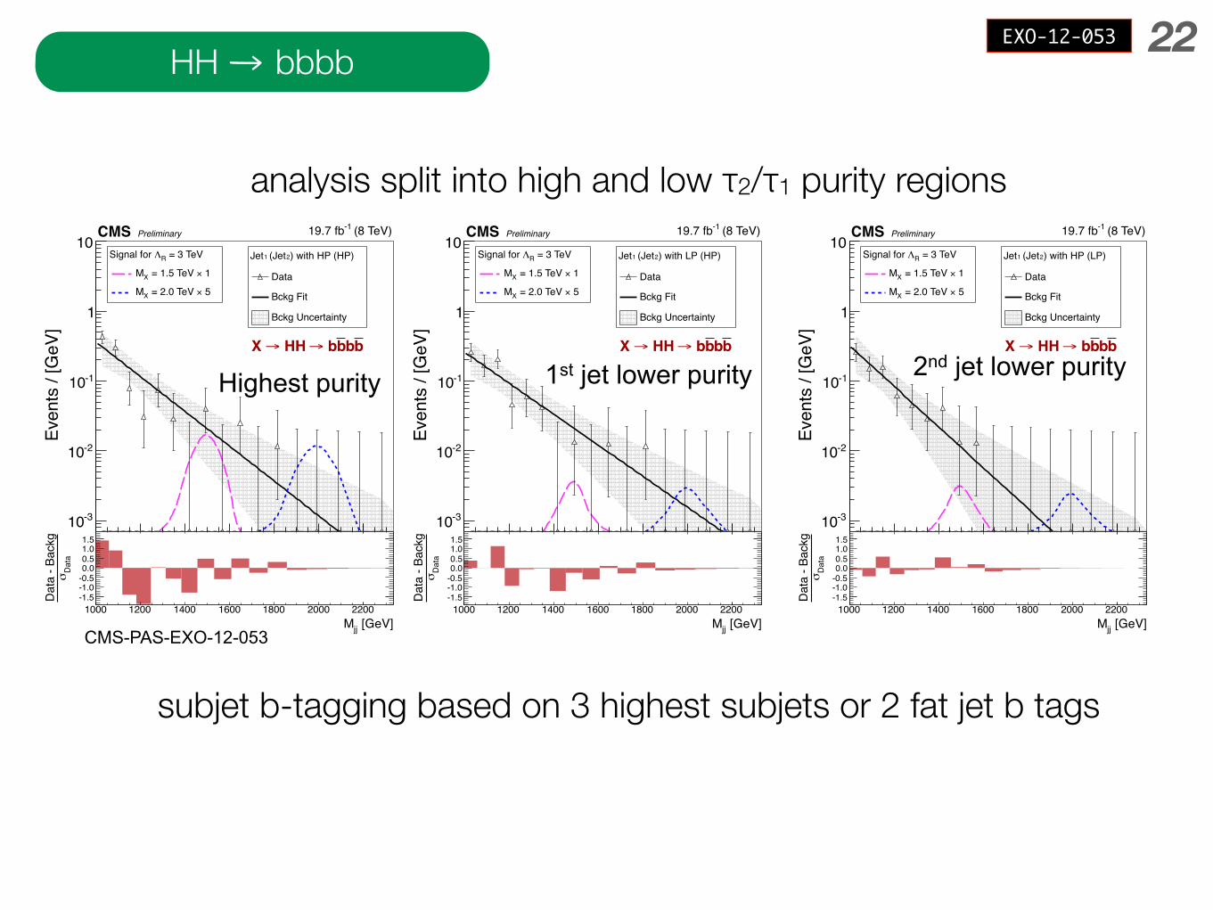
22HH bbbb

[GeV]jjM1000120014001600180020002200

Even

ts /

[GeV

]

-310

-210

-110

1

10) with HP (HP)2 (Jet1Jet

Data

Bckg Fit

Bckg Uncertainty

= 3 TeVRΛSignal for

1× = 1.5 TeV XM

5× = 2.0 TeV XM

bbb b→ HH →X

(8 TeV)-119.7 fbPreliminaryCMS

[GeV]jjM1000 1200 1400 1600 1800 2000 2200

D

ata

σD

ata

- Bac

kg

-1.5-1.0-0.50.00.51.01.5

H(bb)H(bb) resonances – 2


•  Require ≥3 b-tagged subjets in event •  If subjets closer than ΔR<0.3: Require b-tagged fatjet instead of 2 subjets

•  Categorize in purity via τ2/τ1 •  Background estimate is intermediate approach between fitting background

shape in signal region (limited by statistics) and estimation from sideband (limited by understanding of b-tagging fake rate) •  Background shape from pruned jet mass sideband 70<mJ<100 GeV •  Background yield fit together in signal region excluding resonance window

CMS-PAS-EXO-12-053

Highest purity

[GeV]jjM1000120014001600180020002200

Even

ts /

[GeV

]

-310

-210

-110

1

10) with HP (LP)2 (Jet1Jet

Data

Bckg Fit

Bckg Uncertainty


1× = 1.5 TeV XM

5× = 2.0 TeV XM

bbb b→ HH →X


[GeV]jjM1000 1200 1400 1600 1800 2000 2200

D

ata

σD

ata

- Bac

kg

-1.5-1.0-0.50.00.51.01.5

[GeV]jjM1000120014001600180020002200

Even

ts /

[GeV

]

-310

-210

-110

1

10) with LP (HP)2 (Jet1Jet

Data

Bckg Fit

Bckg Uncertainty


1× = 1.5 TeV XM

5× = 2.0 TeV XM

bbb b→ HH →X


[GeV]jjM1000 1200 1400 1600 1800 2000 2200

D

ata

σD

ata

- Bac

kg

-1.5-1.0-0.50.00.51.01.5

1st jet lower purity 2nd jet lower purity

analysis split into high and low τ2/τ1 purity regions

subjet b-tagging based on 3 highest subjets or 2 fat jet b tags

EXO-12-053

23

Findings for spin-0 HH resonances


•  Extra dimension spin-0 radion (ΛR=1 TeV) excluded around 1.2-1.5 TeV

(note: model at edge of validity of narrow width approximation)

HH

Resonance Mass (TeV)1 1.5 2 2.5 3

H(b

b)H(

bb))

(fb)

→ B

R (X

×

σ

-110

1

10

210

310

410 (8 TeV)-119.7 fb

CMSPreliminary Observed

Expectedσ 1 ±Expected σ 2 ±Expected

= 1 TeV)RΛRadion ( = 3 TeV)RΛRadion (

CMS-PAS-EXO-12-053

(GeV)spin-0Xm

500 1000 1500 2000 2500

HH)

(fb)

→ sp

in-0

X→

(pp

σ95

% C

L lim

it on

10

210

310

410

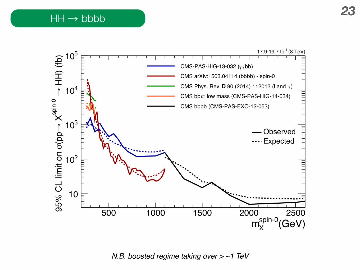
510)bbγγCMS-PAS-HIG-13-032 () - spin-0 bbbCMS arXiv:1503.04114 (b

)γ 90 (2014) 112013 (l and DCMS Phys. Rev. low mass (CMS-PAS-HIG-14-034)ττbCMS b

(CMS-PAS-EXO-12-053)bbbCMS b

ObservedExpected

(8 TeV)-117.9-19.7 fb

HH bbbb

N.B. boosted regime taking over > ~1 TeV

24conclusions and outlook

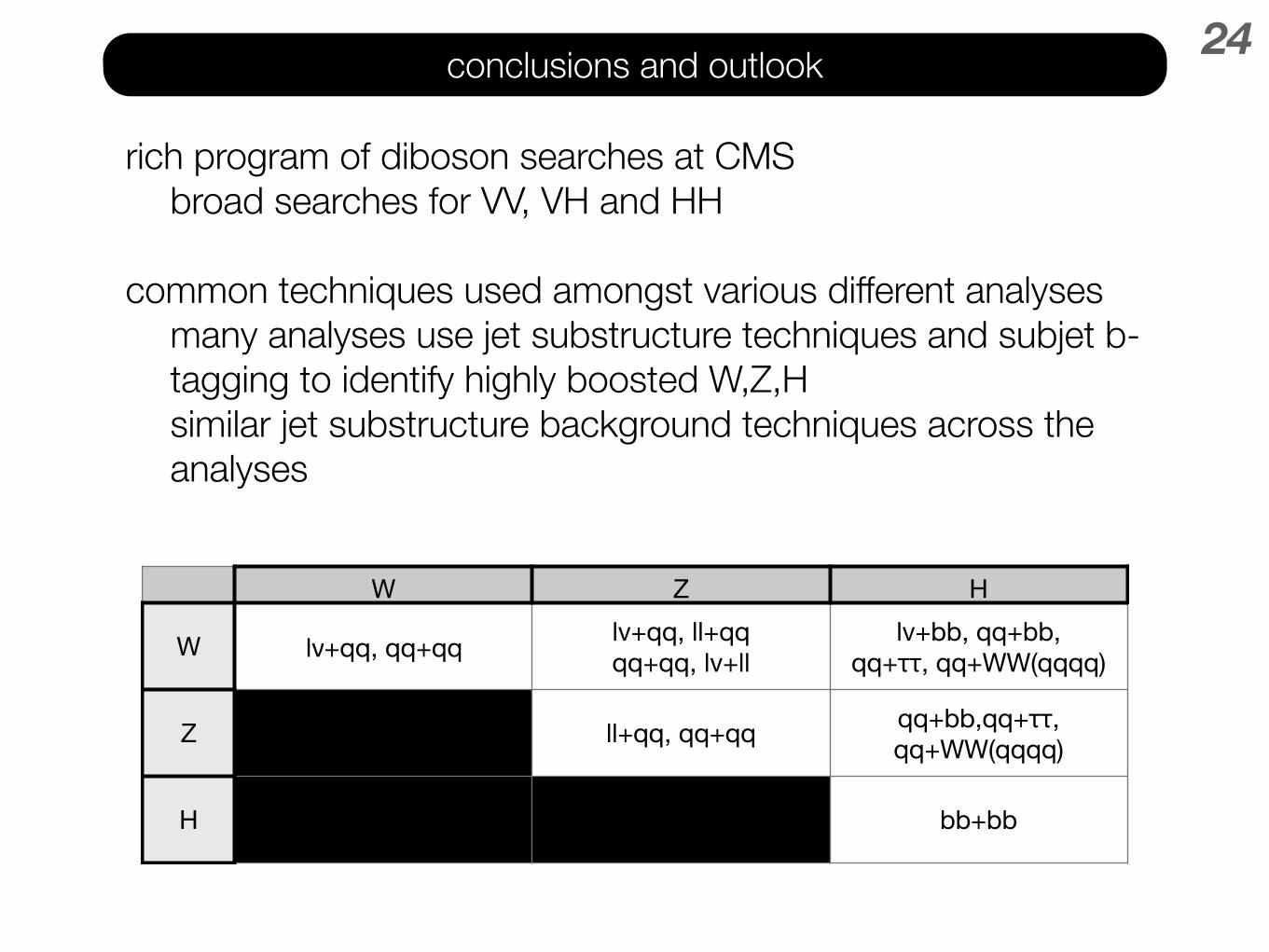
•rich program of diboson searches at CMS •broad searches for VV, VH and HH

•common techniques used amongst various different analyses •many analyses use jet substructure techniques and subjet b-tagging to identify highly boosted W,Z,H

•similar jet substructure background techniques across the analyses

•

W Z H

W lν+qq, qq+qq lv+qq, ll+qqqq+qq, lv+ll

lv+bb, qq+bb,qq+ττ, qq+WW(qqqq)

Z ll+qq, qq+qq qq+bb,qq+ττ, qq+WW(qqqq)

H bb+bb

25conclusions and outlook

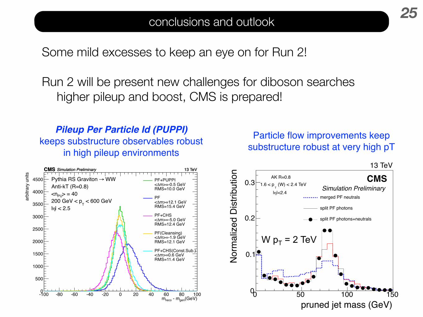
•Some mild excesses to keep an eye on for Run 2!

•Run 2 will be present new challenges for diboson searches •higher pileup and boost, CMS is prepared!

•  To reconstruct high pT jet substructure make full use of ECAL granularity •  Rather than assigning ΣEcalo-Σptrack excess to single photon or neutral

hadron (“merged PF neutrals”) with HCAL granularity •  Split photon excess according to ECAL clusters (“split PF photons”) •  Split hadron excess energy in ECAL+HCAL according to direction and

energy distribution of ECAL clusters (“split PF neutrals”)

jet constituent multiplicity0 50 100 150

Nor

mal

ized

Dis

tribu

tion

0

0.2

0.4

0.6merged PF neutrals

split PF photons

split PF photons+neutrals

AK R=0.8 (W) < 2.4 TeV

T1.6 < p

|<2.4η|

13 TeV

CMSSimulation Preliminary

pruned jet mass (GeV)0 50 100 150

Nor

mal

ized

Dis

tribu

tion

0

0.1

0.2

0.3

merged PF neutrals

split PF photons

split PF photons+neutrals

AK R=0.8 (W) < 2.4 TeV

T1.6 < p

|<2.4η|

13 TeV

CMSSimulation Preliminary

PF improvements for Run II


JME-14-002

W pT = 2 TeV

Particle flow improvements keep substructure robust at very high pT

Pileup Per Particle Id (PUPPI)keeps substructure observables robust

in high pileup environments

(GeV)gen - mrecom-100 -80 -60 -40 -20 0 20 40 60 80 100

arbi

trary

uni

ts

0

500

1000

1500

2000

2500

3000

3500

4000

4500 WW→Pythia RS Graviton Anti-kT (R=0.8)

> = 40PU<n < 600 GeV

T200 GeV < p

| < 2.5 η|

13 TeVCMS Simulation Preliminary

PF+PUPPIm>=-0.5 GeV∆<

RMS=10.0 GeV

PFm>=12.1 GeV∆<

RMS=15.4 GeV

PF+CHSm>=-5.0 GeV∆<

RMS=12.4 GeV

PF(Cleansing)m>=-1.9 GeV∆<

RMS=12.1 GeV

PF+CHS(Const.Sub.)m>=0.6 GeV∆<

RMS=11.4 GeV

13 TeVCMS Simulation Preliminary

26

backup

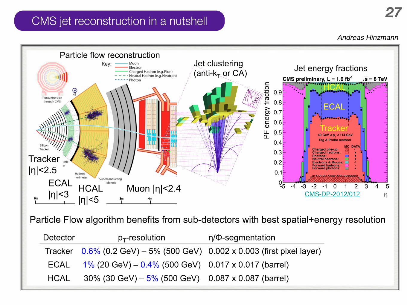
27CMS jet reconstruction in a nutshellJet reconstruction in CMS


HCAL |η|<5

Muon |η|<2.4 ECAL |η|<3

Tracker |η|<2.5

η-5 -4 -3 -2 -1 0 1 2 3 4 5

PF e

nerg

y fra

ctio

n

00.10.20.30.40.50.60.70.80.9

MC DATACharged pile-up: Charged hadrons: Photons: Neutral hadrons: Electrons & Muons: Forward hadrons: Forward photons:

= 8 TeVs-1CMS preliminary, L = 1.6 fb

< 114 GeVT 49 GeV < pTag & Probe method

Detector pT-resolution η/Φ-segmentation Tracker 0.6% (0.2 GeV) – 5% (500 GeV) 0.002 x 0.003 (first pixel layer) ECAL 1% (20 GeV) – 0.4% (500 GeV) 0.017 x 0.017 (barrel) HCAL 30% (30 GeV) – 5% (500 GeV) 0.087 x 0.087 (barrel)

ECAL

Tracker

HCAL

Jet energy fractions

CMS-DP-2012/012

Particle Flow algorithm benefits from sub-detectors with best spatial+energy resolution

Jet clustering (anti-kT or CA)

Particle flow reconstruction

Andreas Hinzmann

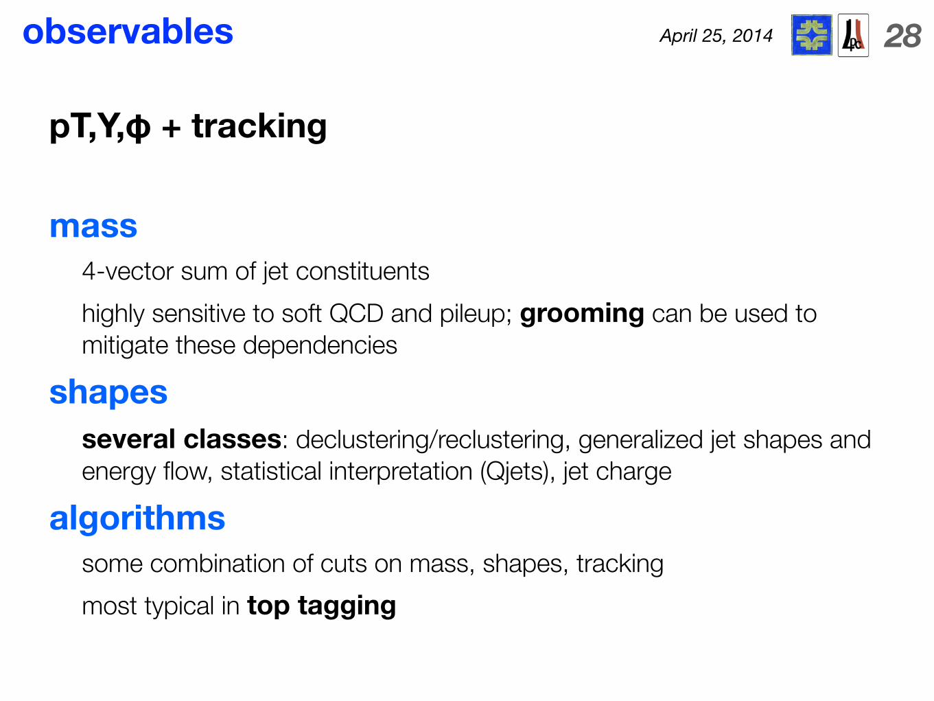
April 25, 2014 28observables

•pT,Y,φ + tracking

•mass •4-vector sum of jet constituents •highly sensitive to soft QCD and pileup; grooming can be used to mitigate these dependencies

•shapes •several classes: declustering/reclustering, generalized jet shapes and energy flow, statistical interpretation (Qjets), jet charge

•algorithms •some combination of cuts on mass, shapes, tracking •most typical in top tagging

1 2

34

1 2

3

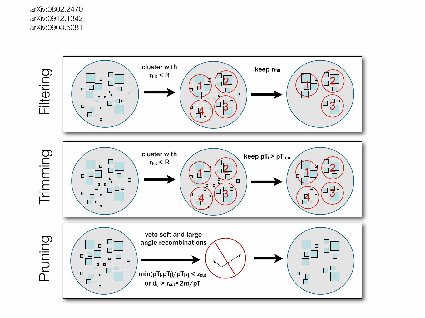
cluster with rfilt < R

keep nfilt

1 2

34

1 2

3


keep pTi > pTfrac

4

veto soft and large angle recombinations

min(pTi,pTj)/pTi+j < zcut or dij > rcut×2m/pT

filtering

trimming

pruning

1 2

34

1 2

3


keep nfilt

1 2

34

1 2

3


keep pTi > pTfrac

4



filtering

trimming

pruning

1 2

34

1 2

3


keep nfilt

1 2

34

1 2

3


keep pTi > pTfrac

4



filtering

trimming

pruning

Trim

ming

Filte

ring

Prun

ing

arXiv:0802.2470 arXiv:0912.1342 arXiv:0903.5081

April 25, 2014 30groomed mass

)PV

Reconstructed vertex multiplicity (N0 2 4 6 8 10 12 14

[GeV

]〉

jet

m〈

20

40

60

80

100

120

140

160 ATLAS = 7 TeVs, -1 Ldt = 1 fb∫Data 2011 LCW jets with R=1.0tanti-k

| < 0.8η < 300 GeV, |Tjet p≤200

No jet grooming =0.3sub=0.01, Rcutf=0.3sub=0.03, Rcutf =0.3sub=0.05, Rcutf=0.2sub=0.01, Rcutf =0.2sub=0.03, Rcutf=0.2sub=0.05, Rcutf

(a) Trimmed anti-kt

: 200 GeV p

jetT <

300 GeV

)PV


[GeV

]〉

1jet

m〈

100

150

200

250

300ATLAS = 7 TeVs, -1 Ldt = 1 fb∫Data 2011

LCW jets with R=1.0tanti-k| < 0.8η < 800 GeV, |

Tjet p≤600

No jet grooming =0.3sub=0.01, Rcutf=0.3sub=0.03, Rcutf =0.3sub=0.05, Rcutf=0.2sub=0.01, Rcutf =0.2sub=0.03, Rcutf=0.2sub=0.05, Rcutf

(b) Trimmed anti-kt

: 600 GeV p

jetT <

800 GeV

)PV


[GeV

]〉

jet

m〈

60

80

100

120

140ATLAS = 7 TeVs, -1 Ldt = 1 fb∫Data 2011

LCW jets with R=1.0tanti-k| < 0.8η < 300 GeV, |

Tjet p≤200

No jet grooming =0.05cut=0.10, zcutR=0.10cut=0.10, zcutR =0.05cut=0.20, zcutR=0.10cut=0.20, zcutR =0.05cut=0.30, zcutR=0.10cut=0.30, zcutR

(c) Pruned anti-kt

: 200 GeV p

jetT < 300 GeV

)PV


[GeV

]〉

1jet

m〈

100

120

140

160

180

200

220

240 ATLAS = 7 TeVs, -1 Ldt = 1 fb∫Data 2011 LCW jets with R=1.0tanti-k

| < 0.8η < 800 GeV, |Tjet p≤600

No jet grooming =0.05cut=0.10, zcutR=0.10cut=0.10, zcutR =0.05cut=0.20, zcutR=0.10cut=0.20, zcutR =0.05cut=0.30, zcutR=0.10cut=0.30, zcutR

(d) Pruned anti-kt

: 600 GeV p

jetT < 800 GeV

)PV


[GeV

]〉

jet

m〈

0

20

40

60

80

100

120

140

160 ATLAS = 7 TeVs, -1 Ldt = 1 fb∫Data 2011C/A LCW jets with R=1.2

| < 0.8η < 300 GeV, |Tjet p≤200

No jet grooming=0.67

fracµ

=0.33frac

µ=0.20

fracµ

(e) Filtered C/A: 200 GeV p

jetT < 300 GeV

)PV


[GeV

]〉

1jet

m〈

50

100

150

200

250

300 ATLAS = 7 TeVs, -1 Ldt = 1 fb∫Data 2011C/A LCW jets with R=1.2

| < 0.8η < 800 GeV, |Tjet p≤600

No jet grooming=0.67

fracµ

=0.33frac

µ=0.20

fracµ

(f) Filtered C/A: 600 GeV p

jetT < 800 GeV

Figure 18. Evolution of the mean uncalibrated jet mass, hmjeti, for jets in the central region|⌘| < 0.8 as a function of the reconstructed vertex multiplicity, N

PV

for jets in the range 200 GeV pjet

T

< 300 GeV (left) and for leading-pjet

T

jets (hmjet

1

i) in the range 600 GeV pjet

T

< 800 GeV(right). (a)-(b) show trimmed anti-kt jets with R = 1.0, (c)-(d) show pruned anti-kt jets withR = 1.0, and (e)-(f) show mass-drop filtered C/A jets with R = 1.2. The error bars indicate thestatistical uncertainty on the mean value in each bin.– 32 –

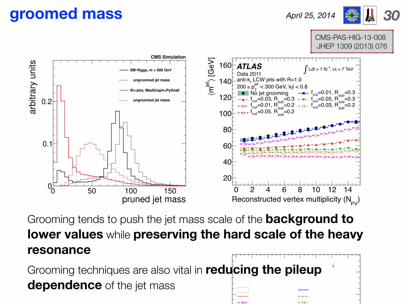
pruned jet mass0 50 100 150

arb

itrary

units

0

0.1

0.2

SM Higgs, m = 600 GeV

ungroomed jet mass

W+Jets, MadGraph+Pythia6

ungroomed jet mass

CMS Simulation

•Grooming tends to push the jet mass scale of the background to lower values while preserving the hard scale of the heavy resonance

•Grooming techniques are also vital in reducing the pileup dependence of the jet mass

CMS-PAS-HIG-13-008 JHEP 1309 (2013) 076

April 25, 2014 31shapes

•Declustering and reclustering •For modern sequential recombination jet algorithms, the jet has a history — a series of 2-to-1 combinations

•examples: mass drop - (msj1/m) , √d12 - first splitting scale of kT algorithm

•Generalized jet shapes •some simple questions: How wide is a jet? How prong-y is a jet? How asymmetric is a jet? How stable is a jet?

•N-subjettiness (τN) [1], how consistent a jet is with having N subjets, ratios are typically used, e.g. τ2/τ1 for W-jets, τ3/τ2 for top jets

•energy correlation functions [2], axis-less version of N-subjettiness •Qjets [3], Exploiting the “quantum” nature of jets •jet charge [4], an oldy but a goody •jet width; pTD; r-cores; planar flow...

[1] Thaler, Van Tilburg, JHEP 1103:015,2011[2] Larkoski, Salam, Thaler, arXiv:1305.0007[3] Ellis et al., PRL 108, 182003 (2012)[4] Krohn et al., Phys. Rev. Lett. 110 (2013) 21200

April 25, 2014 32example: N-subjettiness�58N-subjettiness

N-subjettiness

10

calculations and resummation techniques (see, e.g. recent work in Ref. [29, 30]) compared

to algorithmic methods for studying substructure. Finally, N -subjettiness gives favorable

efficiency/rejection curves compared to other jet substructure methods. While a detailed

comparison to other methods is beyond the scope of this work, we are encouraged by these

preliminary results.

The remainder of this paper is organized as follows. In Sec. 2, we define N -subjettiness

and discuss some of its properties. We present tagging efficiency studies in Sec. 3, where we

use N -subjettiness to identify individual hadronic W bosons and top quarks, and compare

our method against the YSplitter technique [2, 3, 4] and the Johns Hopkins Top Tagger [6].

We then apply N -subjettiness in Sec. 4 to reconstruct hypothetical heavy resonances de-

caying to pairs of boosted objects. Our conclusions follow in Sec. 5, and further information

appears in the appendices.

2. Boosted Objects and N-subjettiness

Boosted hadronic objects have a fundamentally different energy pattern than QCD jets

of comparable invariant mass. For concreteness, we will consider the case of a boosted

W boson as shown in Fig. 1, though a similar discussion holds for boosted top quarks or

new physics objects. Since the W decays to two quarks, a single jet containing a boosted

W boson should be composed of two distinct—but not necessarily easily resolved—hard

subjets with a combined invariant mass of around 80 GeV. A boosted QCD jet with an

invariant mass of 80 GeV usually originates from a single hard parton and acquires mass

through large angle soft splittings. We want to exploit this difference in expected energy

flow to differentiate between these two types of jets by “counting” the number of hard lobes

of energy within a jet.

2.1 Introducing N-subjettiness

We start by defining an inclusive jet shape called “N -subjettiness” and denoted by τN .

First, one reconstructs a candidate W jet using some jet algorithm. Then, one identifies

N candidate subjets using a procedure to be specified in Sec. 2.2. With these candidate

subjets in hand, τN is calculated via

τN =1

d0

!

k

pT,k min {∆R1,k,∆R2,k, · · · ,∆RN,k} . (2.1)

Here, k runs over the constituent particles in a given jet, pT,k are their transverse momenta,

and ∆RJ,k ="

(∆η)2 + (∆φ)2 is the distance in the rapidity-azimuth plane between a

candidate subjet J and a constituent particle k. The normalization factor d0 is taken as

d0 =!

k

pT,kR0, (2.2)

where R0 is the characteristic jet radius used in the original jet clustering algorithm.

It is straightforward to see that τN quantifies how N -subjetty a particular jet is, or

in other words, to what degree it can be regarded as a jet composed of N subjets. Jets

– 3 –(a)

0 0.5 1 1.5

4.5

5

5.5

6

Boosted Top Jet, R = 0.8

η

φ

(b)

(c)

−1.5 −1 −0.5 0−0.15

0.35

0.85

1.35

1.75Boosted QCD Jet, R = 0.8

η

φ

(d)

Figure 4: Left: Decay sequences in (a) tt and (c) dijet QCD events. Right: Event displays for(b) top jets and (d) QCD jets with invariant mass near mtop. The labeling is similar to Fig. 1,though here we take R = 0.8, and the cells are colored according to how the jet is divided intothree candidate subjets. The open square indicates the total jet direction, the open circles indicatethe two subjet directions, and the crosses indicate the three subjet directions. The discriminatingvariable τ3/τ2 measures the relative alignment of the jet energy along the crosses compared to theopen circles.

a b jet and a W boson, and if the W boson decays hadronically into two quarks, the top jet

will have three lobes of energy. Thus, instead of τ2/τ1, one expects τ3/τ2 to be an effective

discriminating variable for top jets. This is indeed the case, as sketched in Figs. 4, 5, 6,

and 7.

– 7 –

☐ = τ1

◯ = τ2

× = τ3

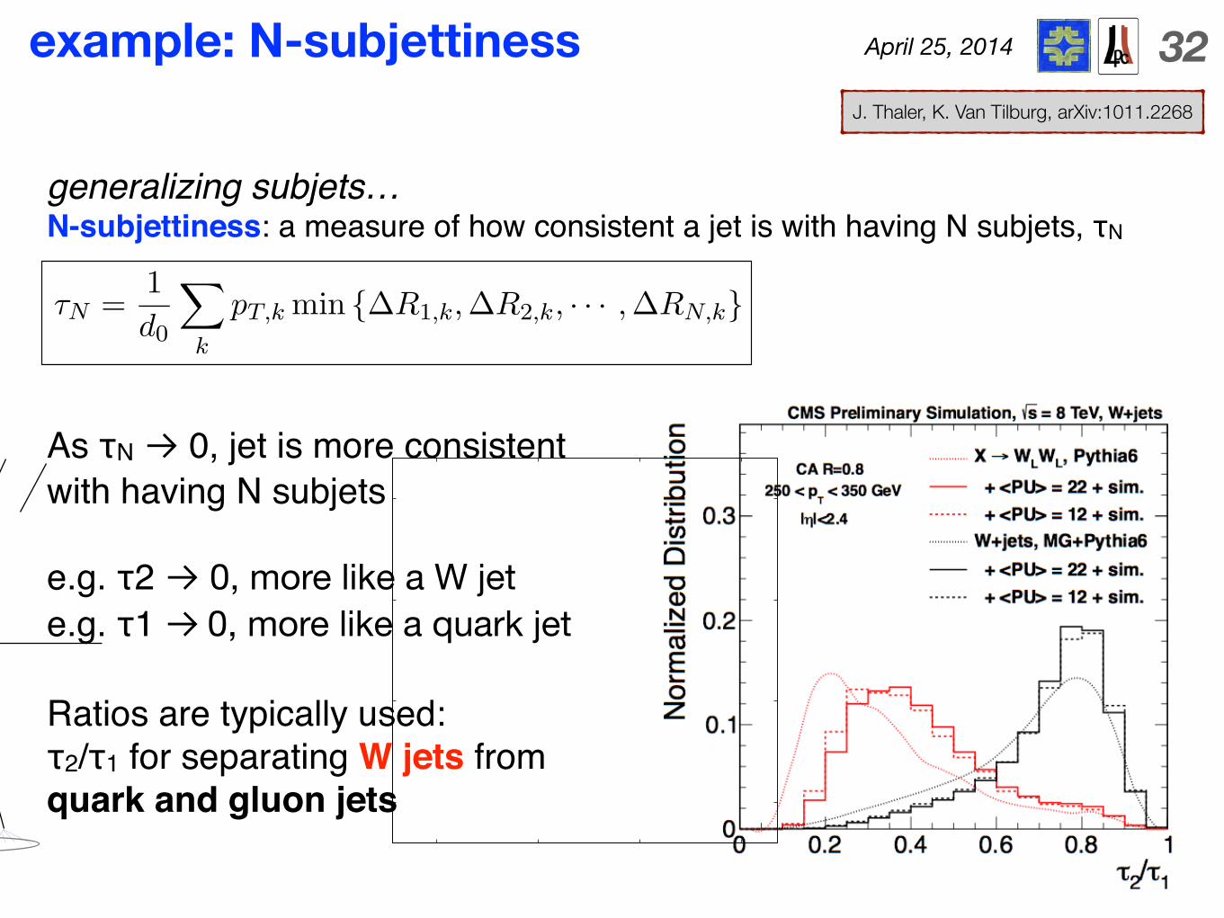
generalizing subjets...N-subjettiness: a measure of how consistent a jet is with having N subjets, τN

k, sum over particles in the jetN subjet axes for computing τN

calculations and resummation techniques (see, e.g. recent work in Ref. [29, 30]) compared

to algorithmic methods for studying substructure. Finally, N -subjettiness gives favorable

efficiency/rejection curves compared to other jet substructure methods. While a detailed

comparison to other methods is beyond the scope of this work, we are encouraged by these

preliminary results.

The remainder of this paper is organized as follows. In Sec. 2, we define N -subjettiness

and discuss some of its properties. We present tagging efficiency studies in Sec. 3, where we

use N -subjettiness to identify individual hadronic W bosons and top quarks, and compare

our method against the YSplitter technique [2, 3, 4] and the Johns Hopkins Top Tagger [6].

We then apply N -subjettiness in Sec. 4 to reconstruct hypothetical heavy resonances de-

caying to pairs of boosted objects. Our conclusions follow in Sec. 5, and further information

appears in the appendices.

2. Boosted Objects and N-subjettiness

Boosted hadronic objects have a fundamentally different energy pattern than QCD jets

of comparable invariant mass. For concreteness, we will consider the case of a boosted

W boson as shown in Fig. 1, though a similar discussion holds for boosted top quarks or

new physics objects. Since the W decays to two quarks, a single jet containing a boosted

W boson should be composed of two distinct—but not necessarily easily resolved—hard

subjets with a combined invariant mass of around 80 GeV. A boosted QCD jet with an

invariant mass of 80 GeV usually originates from a single hard parton and acquires mass

through large angle soft splittings. We want to exploit this difference in expected energy

flow to differentiate between these two types of jets by “counting” the number of hard lobes

of energy within a jet.

2.1 Introducing N-subjettiness

We start by defining an inclusive jet shape called “N -subjettiness” and denoted by τN .

First, one reconstructs a candidate W jet using some jet algorithm. Then, one identifies

N candidate subjets using a procedure to be specified in Sec. 2.2. With these candidate

subjets in hand, τN is calculated via

τN =1

d0

!

k

pT,k min {∆R1,k,∆R2,k, · · · ,∆RN,k} . (2.1)

Here, k runs over the constituent particles in a given jet, pT,k are their transverse momenta,

and ∆RJ,k ="

(∆η)2 + (∆φ)2 is the distance in the rapidity-azimuth plane between a

candidate subjet J and a constituent particle k. The normalization factor d0 is taken as

d0 =!

k

pT,kR0, (2.2)

where R0 is the characteristic jet radius used in the original jet clustering algorithm.

It is straightforward to see that τN quantifies how N -subjetty a particular jet is, or

in other words, to what degree it can be regarded as a jet composed of N subjets. Jets

– 3 –

Ratios of τN are traditionally used for discriminating signal

from background

J. Thaler, K. Van Tilburg, arXiv:1011.2268

generalizing subjets…N-subjettiness: a measure of how consistent a jet is with having N subjets, τN

As τN → 0, jet is more consistent with having N subjets

e.g. τ2 → 0, more like a W jet e.g. τ1 → 0, more like a quark jet

Ratios are typically used:τ2/τ1 for separating W jets from quark and gluon jets

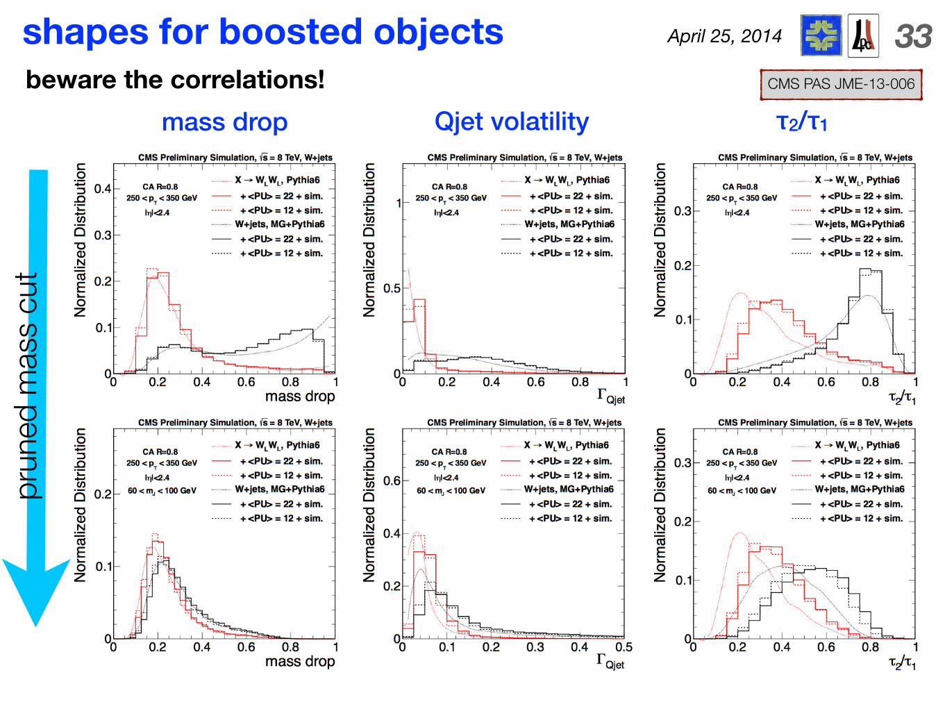
April 25, 2014 33shapes for boosted objects

mass drop Qjet volatility τ2/τ1

prun

ed m

ass

cut

beware the correlations! CMS PAS JME-13-006

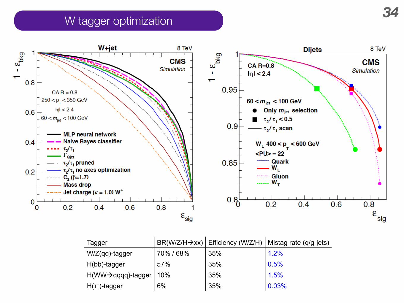
34W tagger optimization

W-tagger optimization


arXiv:1410.4227

W/Z/H tagging comparison


•  Compare Run I W/Z/H taggers at 35% efficiency working point

•  H(bb) can be discriminated from background by a factor >2 better than W(qq)/Z(qq)

Tagger BR(W/Z/H!xx) Efficiency (W/Z/H) Mistag rate (q/g-jets) W/Z(qq)-tagger 70% / 68% 35% 1.2% H(bb)-tagger 57% 35% 0.5% H(WW!qqqq)-tagger 10% 35% 1.5% H(ττ)-tagger 6% 35% 0.03%

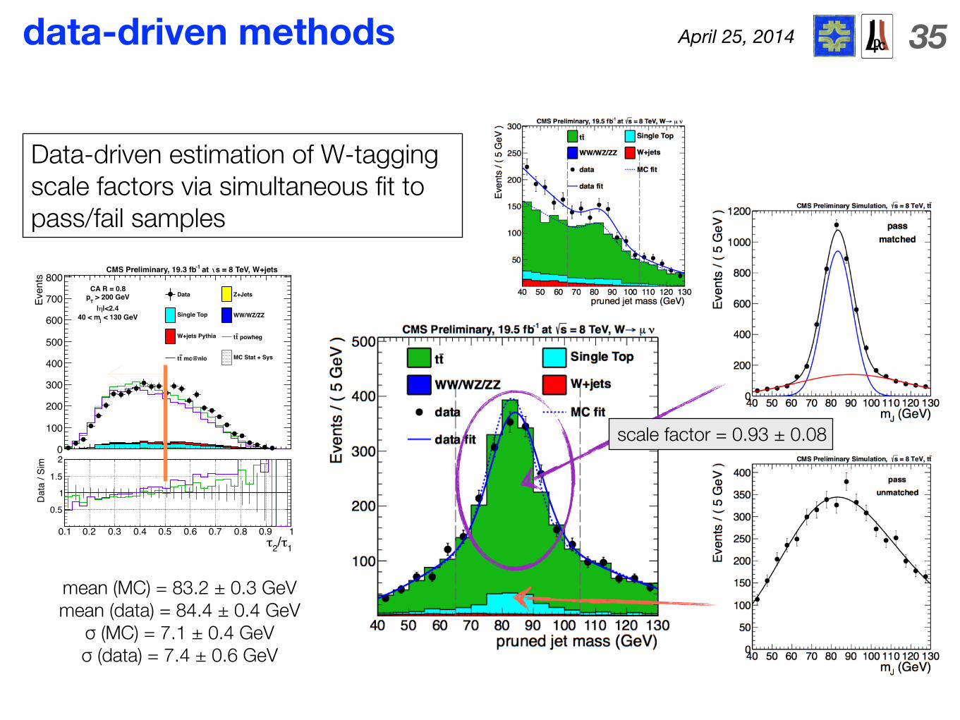
April 25, 2014 35data-driven methodsEv

ents

0

100

200

300

400

500

600

700

800Data Z+Jets

Single Top WW/WZ/ZZ

W+jets Pythia powhegtt

mc@nlott MC Stat + Sys

= 8 TeV, W+jetss at -1CMS Preliminary, 19.3 fb

CA R = 0.8 > 200 GeV

Tp

|<2.4η| < 130 GeVj40 < m

1τ/2τ0.1 0.2 0.3 0.4 0.5 0.6 0.7 0.8 0.9 1

Dat

a / S

im

0.5

1

1.5

2

Data-driven estimation of W-tagging scale factors via simultaneous fit to pass/fail samples

mean (MC) = 83.2 ± 0.3 GeV mean (data) = 84.4 ± 0.4 GeV

σ (MC) = 7.1 ± 0.4 GeV σ (data) = 7.4 ± 0.6 GeV

scale factor = 0.93 ± 0.08

Documents

Searches for Diboson Resonances at CMS - indico.bnl.gov · high mass resonances for diboson resonances 3 are a staple of new physics searches Outline of the talk 2 11 Aug 2015 Andreas