Search With Adverse Selection

http://www.econometricsociety.org/

Econometrica, Vol. 84, No. 1 (January, 2016), 243–315

SEARCH WITH ADVERSE SELECTION

STEPHAN LAUERMANNUniversity of Bonn, 53115 Bonn, Germany

ASHER WOLINSKYNorthwestern University, Evanston, IL 60208-2600, U.S.A.

The copyright to this Article is held by the Econometric Society. It may be downloaded,printed and reproduced only for educational or research purposes, including use in coursepacks. No downloading or copying may be done for any commercial purpose without theexplicit permission of the Econometric Society. For such commercial purposes contactthe Office of the Econometric Society (contact information may be found at the websitehttp://www.econometricsociety.org or in the back cover of Econometrica). This statement mustbe included on all copies of this Article that are made available electronically or in any otherformat.


Econometrica, Vol. 84, No. 1 (January, 2016), 243–315

SEARCH WITH ADVERSE SELECTION

BY STEPHAN LAUERMANN AND ASHER WOLINSKY1

This paper analyzes a sequential search model with adverse selection. We study in-formation aggregation by the price—how close the equilibrium prices are to the full-information prices—when search frictions are small. We identify circumstances underwhich prices fail to aggregate information well even when search frictions are small. Wetrace this to a strong form of the winner’s curse that is present in the sequential searchmodel. The failure of information aggregation may result in inefficient allocations.

KEYWORDS: Adverse selection, winner’s curse, search theory, auctions, informationaggregation.

1. INTRODUCTION

THIS PAPER analyzes a sequential search model with asymmetric information ofthe common-value variety. The main objective is to understand how the com-bination of search activity and information asymmetry affects prices and wel-fare. We specifically study the extent of information aggregation by the price—that is, how close the equilibrium transaction prices are to the full-informationprices—when search frictions are small. Roughly speaking, we conclude thatinformation is aggregated less well in the sequential search model than it isin a standard common-value auction. In fact, when search frictions are small,the equilibrium prices may be entirely independent of the common value ofthe transaction, even when there are exceedingly informative signals. We tracethis failure of information aggregation to a stronger form of the winner’s cursethat arises with sequential search. This is a central insight of this paper. Wealso look at the efficiency perspective and relate the extent of potential ineffi-ciencies to the informativeness of the signal technology available to the unin-formed. In the analysis leading to these results, we develop a simple measurefor the relative informativeness of signals.

The searching agent (the buyer) samples sequentially, at a cost, trading part-ners (sellers) for a transaction that involves information asymmetry. The buyerhas private information (type) w ∈ {1�2� � � � �m} that determines the cost of thetransaction cw for any seller, where c1 < · · ·< cm. Upon being sampled, a sellerobserves a noisy signal of the cost but not the buyer’s search history. Then thebuyer and that seller bargain over the price. The outcome of the bargaining isaffected by the seller’s belief resulting from updating the common prior over

1We are grateful to the co-editor, the anonymous referees, Larry Samuelson, Lones Smith, andGábor Virág for their comments and to Qinggong Wu, Daniel Fershtman, and Teddy Mekonnenfor excellent research assistance. The authors gratefully acknowledge support from the NationalScience Foundation under Grants SES-1123595 and SES-1061831. The authors also thank theHausdorff Research Institute (HIM) in Bonn, where parts of this paper were written, for hospi-tality.

© 2016 The Econometric Society DOI: 10.3982/ECTA9969



http://dx.doi.org/10.3982/ECTA9969

244 S. LAUERMANN AND A. WOLINSKY

the buyer’s type with the information contained in being sampled and in theobserved signal. Different sellers observe different, conditionally independentsignals. This induces the buyer to search for sellers who would receive a favor-able signal so as to trade at a lower price. The strength of this incentive and,hence, the resulting search intensity generally vary across the different types ofthe buyer and this feeds back into the sellers’ beliefs. The equilibrium conceptis perfect Bayesian equilibrium. Each agent’s behavior is optimal given the be-havior of others, and sellers’ beliefs are Bayesian updates of the common priorgiven the signals and the understanding of the buyer’s equilibrium behavior.The effect of the buyer’s equilibrium search behavior on sellers’ beliefs and,hence, on the price is the main element that distinguishes the nature of priceformation and information aggregation in this search environment from thatin a related auction environment.

Although our model is not formulated with a specific application in mind, itprovides a general model for a number of important scenarios. One concretescenario is that of the procurement of a repair service by an individual (thebuyer), who searches among potential providers (the sellers). Another scenariois that of a loan market. Here, the buyer is a potential borrower who seeksfunding for an investment of uncertain quality and the sellers are potentiallenders.2 Finally, our model also captures the standard examples of marketsfor “lemons,” that is, sales of objects of uncertain quality by an informed seller.For this interpretation, we only have to reverse the roles of those we call buyerand sellers.

Information aggregation by prices is a central topic of the economic theoryof markets.3 In the context of the present model, the information dispersedamong the sellers is aggregated (nearly) perfectly if the price at which thetransaction takes place is (nearly) equal to the true cost; the price does notaggregate any information if it is independent of the true cost. It is reasonableto expect that a large sampling cost would impede the search and prevent sig-nificant information aggregation. We therefore focus on a nearly frictionlessenvironment in which the sampling cost is small. The extent of information ag-gregation by the equilibrium price is related of course to the informativeness ofthe signal technology. A more detailed account of this relationship is discussednext.

Let Fw be the distribution of the signal x observed by a seller upon encoun-tering the buyer of type w ∈ {1� � � � �m}. Let fw be its density and let [x�x] be

2Of course, any such specific application would require further thought about the details. Forexample, for certain kinds of individual loans, lenders have access to a credit score that mayreflect past loan applications by the borrower.

3The term information aggregation is used here to describe the collection of information thatis dispersed among the sellers and the reflection of this information in prices. This is of courserelated to the question of whether the equilibrium prices are pooling or separating, and occasion-ally we use these terms as well. However, the term aggregation emphasizes the coalescence ofdispersed information, which is the focus of our paper.

SEARCH WITH ADVERSE SELECTION 245

its common support. For w< w, the likelihood ratio fw(x)/fw(x) is decreasingso that low realizations of x indicate a higher likelihood of low-cost types. Thelikelihood ratio is already a measure of informativeness: if fw(x)/fw(x) attainslarge values, then the signal is informative in the sense that such realizationssharply distinguish w from w. Our results on information aggregation cannotbe explained in terms of the magnitude of the likelihood ratio alone. They alsorely on another measure,

λw�w = limx→x

fw(x)

fw(x)

− lnFw(x)� w < w�

The measure λw�w may take any value in [0�∞]. Larger values of λw�w meangreater power of distinguishing w from w. Since − lnFw(x) → ∞ as x → x,it follows that λw�w = 0 if fw(x)

fw(x)is bounded or if fw(x)

fw(x)→ ∞ more slowly than

− lnFw(x) as x → x. A value λw�w > 0 means that fw(x)

fw(x)→ ∞ sufficiently fast as

x→ x.It is shown that if λw�w+1 = ∞ for all w <m, then equilibrium prices aggre-

gate the information perfectly: pw = cw, where pw is type w’s expected equi-librium price in the limit as the sampling cost becomes negligible. If λ1�m = 0,then no information is aggregated at all: the buyer trades at the same priceindependently of the type and pw equals ex ante expected cost for all w. Thus,information aggregation requires not only that signals are unboundedly infor-mative, but that such signals are sufficiently likely to occur. Generically, in asense that we make precise later, the measures λw�w are either 0 or ∞. There-fore, these two extremes of perfect separation and complete pooling are notknife-edge cases.

A range of intermediate situations that exhibit imperfect information aggre-gation lies between the two extremes described above. We illustrate the generalform of the expected equilibrium prices (in the limit, as the search cost be-comes negligible) in Figure 1. The two extreme cases of complete pooling andcomplete separation mentioned above are illustrated by panel A and panel C.In panel A, the limit prices are flat at the level of the ex ante expected cost. Inpanel C, the limit prices coincide with the graph of cw. Panel B illustrates anintermediate case with partial pooling.

In general, the set of types is shown to be partitioned into “pools” of adjacenttypes. All types in each pool, except perhaps the highest type in the pool, paythe same expected price, which is a certain weighted average of the costs of thetypes in the pool.4 The pools are separated from each other in the sense thatif w < w and they are in different pools, then in the limit, type w trades withprobability 1 at a price above pw and type w trades with probability 1 at a price

4The highest type in the pool pays the same price with some probability (possibly 1) and paysa price near its own cost with the complementary probability.


FIGURE 1.—Example showing limit equilibrium prices. In panel A, all types are pooled at theex ante expected costs. In panel B, types {1�2} are pooled on a common price. Types {3�4�5�6}are also pooled, with type 6 paying a mixture of the common price and c6. Types 7 and 8 areseparated. Panel C shows complete separation.

below pw. If type w is in a pool by itself, then pw = cw, that is, the equilibriumprice aggregates buyer type w’s information perfectly. If a pool contains severaltypes, their information is not aggregated perfectly by the price. The two ex-treme cases of complete pooling (panel A) and complete separation (panel C)are the special cases in which there is only one pool or all pools are singletons.In panel B, the pools are [{1�2}� {3�4�5�6}� {7}� {8}].

The relationship between the measure λw�w and the shape of the pools is thatλw�w = ∞ implies that w and w are in separate pools, while in the generic case,λw�w = 0 if w and w are in the same pool. The failure of prices to aggregate theinformation perfectly is caused by the incentives for higher cost buyer types tomimic the search behavior of lower cost types, which diminishes the informa-tive value of signals. In a sense, λw�w captures how hard it is for type w to mimictype w.

The basic features of the present model resemble those of a standardcommon-value (procurement) auction. Just imagine that instead of samplingsellers sequentially, the buyer assembles a group of sellers for an auction. Al-though a number of differences exist between the models, the crucial differ-ence is between the endogenous sampling of sellers in the search model andthe exogenously fixed set of bidders in the auction model. We compare our re-sults to their counterparts in such a procurement auction with n sellers/biddersand the same signal structure.

Results by Milgrom (1979) and Wilson (1977) imply that the equilibriumwinning bid in this auction aggregates the information perfectly in the limit asn → ∞ if and only if limx→x fw(x)/fw+1(x) = ∞ for all w < m. In our searchmodel, the number of sellers encountered by the buyer is endogenous, so insome sense the counterpart of the large n in the auction is a small sampling cost


(that would induce the sampling of many sellers). As mentioned above, perfectinformation aggregation in the search model (in the limit as the sampling costbecomes negligible) requires a stronger condition, λw�w+1 = ∞ for all w <m,on the rate at which the informativeness of signals increases as x→ x. Indeed,the equilibrium of the search model may exhibit complete pooling in the limit,even when limx→x fw(x)/fw+1(x)= ∞ for all w<m.

In contrast, the auction equilibrium never involves complete pooling in thelimit, even when limx→x fw(x)/fw+1(x) < ∞ for all w. In other words, in thecounterpart of Figure 1 for the large auction, the schedule is always strictly in-creasing, even when prices do not converge to costs. In this sense, the searchmodel aggregates information more poorly than the corresponding auctionmodel. The reason for this difference is that, in the standard auction model, thenumber of sellers/bidders is fixed and independent of the true cost, whereas inthe search model, this number is endogenous and dependent on the true cost.This exacerbates the winner’s curse in the search model relative to its coun-terpart in the corresponding auction model and impedes the aggregation ofinformation by prices.

We also consider the welfare implications. In our base model, trade is alwaysbeneficial and always takes place. Hence, welfare coincides with the negativeof the accumulated search costs because the price is just a transfer. We evalu-ate welfare in the limit as the sampling cost goes to zero. In the generic case,when there is either complete separation or complete pooling, then the accu-mulated search costs are zero. We demonstrate that this is not always the caseand accumulated search cost can be nonzero when there is partial separation.In a variation on the basic model introduced in Section 5, the volume of tradeis also determined endogenously. Here, imperfect aggregation of informationmight result in an inefficient volume of trade, so that even though the totalsearch cost is zero in the limit, the allocation might be inefficient.

A key feature of the model and the environments it represents is the sellers’inability to observe the buyer’s history. This is a natural assumption in someimportant settings. For example, while venture capitalists are aware that aninventor may have applied for funding elsewhere, they do not generally ob-serve how many other venture capitalists an inventor has already contacted orwhat may have happened in those prior meetings. Obviously, this leaves outinteresting environments in which significant parts of the searcher’s history areobservable.

1.1. Related Literature

This paper is related to three bodies of work. One deals with the questionof information aggregation in the interaction of a large group of players. Wehave already mentioned Milgrom (1979) and Wilson (1977), who address thisquestion in the context of a single-unit auction. Feddersen and Pesendorfer(1997) and Duggan and Martinelli (2001) consider information aggregation in


the context of a voting model, Smith and Sørenson (2000) consider it in thecontext of social learning, and Pesendorfer and Swinkels (1997) consider it inthe context of a multi-unit auction.

Another related body of work focuses on search with adverse selection, forexample, Inderst (2005), Moreno and Wooders (2010), and Guerrieri, Shimer,and Wright (2010). While these papers use different models and investigatedifferent questions, nevertheless they do share with our paper the idea thatin a search model, the distribution of types is determined endogenously. Forexample, in Inderst (2005), the distribution of types adjusts to sustain theRothschild–Stiglitz best separating outcome as an equilibrium, which wouldnot necessarily be the case for an arbitrary exogenous distribution of types.

A few papers fall within the intersection of these two bodies of literature.Wolinsky (1990) and Blouin and Serrano (2001) show that in a two-sidedsearch model with binary signals and actions, information is not aggregatedperfectly even as frictions become negligible. Duffie and Manso (2007) andDuffie, Malamud, and Manso (2009) characterize information percolation inmarkets in which agents truthfully exchange their information with each otherwhenever they are matched. However, while those papers study private infor-mation about a marketwide state of nature, in our model, the private informa-tion is idiosyncratic to each buyer.

A third body of related literature concerns dynamic trade with adverse se-lection. One strand studies the separation of quality types through differencesin preferences over the timing and probability of trade. Owing to a single-crossing condition, high-quality types trade more slowly. This strand includesEvans (1989), Vincent (1989), Deneckere and Liang (2006), and Hörner andVieille (2009). Another strand studies the effect of the gradual resolution ofuncertainty through public signals; for this, see Bar-Isaac (2003), Kremer andSkrzypacz (2007), and Daley and Green (2012), all three of which expand onSwinkels (1999). In contrast, in our model, the preferences of different typesover the timing of trade are identical and we document the limited separa-bility of types through private signals. Zhu (2012) models opaque financialover-the-counter markets using a variation of our model with a finite num-ber of sellers and no search costs. These differences (and some other featuresof the trading process) set these models apart—Zhu’s model resembles morea sort of an auction with two prices than a search model of the sort we areconsidering. Accordingly, the analysis and the results are significantly differ-ent across these models. In particular, Zhu’s model generates a weaker win-ner’s curse than a standard auction and, hence, aggregates information better,whereas a central insight of our analysis concerns the stronger winner’s cursearising in the search model and its inhibiting effect on information aggrega-tion.


2. THE MODEL AND PRELIMINARY ANALYSIS

2.1. The Setup

A single buyer samples sequentially among a large number of sellers insearch of a single transaction. The gross value for the buyer of transacting witha seller is u. The buyer incurs a sampling cost s > 0 for each seller sampled.The set of sellers is the interval [0�1]. The buyer’s draws from this set are in-dependent and uniformly distributed.

All sellers incur the same cost for the transaction. This cost depends onthe buyer’s type w ∈ W = {1�2� � � � �m} and is denoted by cw, with c1 < c2 <· · ·< cm. The prior probability of type w is ρw. The buyer knows w but the sell-ers do not. It is assumed that u > cm, so that trade is efficient for all types ofthe buyer.5 The ex ante expected cost is Eρ[c] =∑m

i=1 ρici.Upon meeting the buyer, the seller obtains a signal x ∈ X = [x�x] from a

distribution with a cumulative distribution function (c.d.f.) Fw that depends onthe buyer’s type w and has a continuously differentiable density fw, which isstrictly positive on (x�x).6 The likelihood ratio fw(x)

fv(x)is strictly decreasing in x

on (x�x) for all w < v (monotone likelihood ratio property (MLRP)), so thata lower signal indicates a strictly higher likelihood of lower types. The implieddistribution of the likelihood ratios satisfies two further assumptions. First, theexpected likelihood ratio is finite,

E

[f1

fm

∣∣∣w = 1]

=∫ x

x

f1(x)

fm(x)f1(x)dx <∞�(1)

Second, for all types i� j, with i < j,

limx→x

− d

dx

(fi(x)

fj(x)

)fi(x)

Fi(x)

(2)

exists, allowing for it to be ∞ as well.7 By L’Hôpital’s rule, (2) is equal to theλij measure defined in the Introduction and discussed later.8

After a seller is sampled and has observed the realization of the signal, bar-gaining unfolds: Nature draws a price p ∈ [0�u] from a c.d.f. G that has a

5We relax this assumption in Section 5.6We allow x = −∞ and x= +∞.7The finiteness of the expected likelihood ratio precludes a positive probability of perfectly

informative signals, as considered in particular by Wilson (1977). Expression (2) will be discussedextensively; see especially Section 6.

8We are thankful to a referee for suggesting the expression in the Introduction for the λij

measure.


continuous density g strictly positive on [0�u]. Given the price, first the sellerand then the buyer decide whether to accept it.9 Acceptance by both partiesends the game. Rejection by either party terminates this match and the buyercontinues sampling.

The “random proposals” bargaining model has been used in the related lit-erature by Wilson (2001) and Compte and Jehiel (2010). It provides a robustmodel of bargaining with asymmetric information that avoids the complica-tions of dealing with off-path beliefs. We discuss this modeling choice and al-ternative bargaining models in Section 8.

Before making the acceptance decision, the sampled seller observes boththe signal and the price, but does not observe anything else about the historyof the game. In particular, the seller does not observe how many other sellersthe buyer has already sampled. The buyer observes the price, and she knowsher private history. It does not matter whether or not the buyer observes theseller’s signal.

A history of the process records the sequence of all encountered sellers, sig-nal realizations, prices, and acceptance decisions up to a certain point. A ter-minal history is a history that either ends with a trade or an infinite history withno trade.

A finite terminal history determines a terminal outcome (nt�pt�xt� jt),where nt is the total number of sellers sampled by the buyer, and pt , xt , andjt are the price, the signal, and the identity, respectively, of the seller in theterminal trade.

The payoff for the buyer of type w after a finite terminal history is

u−pt − nts;the payoff after an infinite history is −∞.

The payoff for seller jt from transacting with the buyer with type w is

pt − cw;the payoffs are zero for all other sellers.

A pure strategy for seller j is an acceptance set of prices Aj(x) ⊂ [0�u] foreach signal value, since the current signal is all the seller observes. A purestrategy for a buyer with type w is an acceptance set for any history ϕ, denotedBw(ϕ) ⊂ [0�u].

The strategy profile (B�A) = ((Bw)w∈W � (Aj)j∈[0�1]), together with the priorover the set of types W , induces a distribution on the set of terminal historiesand, hence, over terminal outcomes. The expected payoff of the buyer is

Vw(B�A)= u−E[pt |w;B�A]− sE

[nt|w;B�A]�

9This order of decisions avoids signaling problems that arise if the buyer decides first.


where the expectation is taken with respect to the said distribution. We abbre-viate Vw = Vw(B�A).10

We assume that the sampling costs are small enough such that

u≥∫ u

cm

pg(p)

1 −G(cm)dp+ s

1 −G(cm)�(3)

With this assumption, the buyer’s payoff is positive even if the sellers acceptonly prices that are above cm.

Given a strategy profile (B�A), let Π(w|x) =Π(w|x;B�A) denote a seller’sbelief11 that the buyer’s type is w, conditional on that seller being sampled andobserving signal x.

Equilibrium

A (perfect-Bayesian) equilibrium consists of a strategy profile (B�A) and abelief Π such that:

(i) After any history ϕ, Bw maximizes the expected payoff of the buyer oftype w given A.

(ii) For any signal realization x, Aj(x) maximizes seller j’s expected profitgiven B and Π(w|x).

(iii) The belief Π(w|x) is consistent with Bayesian updating for all x.

2.2. Equilibrium Strategies and Beliefs

Buyer’s Equilibrium Strategy

Recall that Vw is buyer w’s expected payoff. Since the distributions of priceoffers and the sellers’ behavior are independent of the history, Vw is also thebuyer’s expected continuation payoff from any point on forward. It follows bya standard argument that, for any history, the buyer’s optimal decision is toaccept a price if and only if p ≤ u − Vw. Thus, for all ϕ, Bw(ϕ) = [0�u − Vw].That is, the buyer’s equilibrium strategy is stationary and described by a cutoff,u−Vw. Therefore, we omit the argument ϕ and henceforth write Bw(ϕ) as Bw.

10Here and henceforth, whenever we introduce a magnitude that depends on the profile(B�A)—such as Vw(B�A) and E[·|w;B�A]—we will indicate it once and then drop the (B�A)argument. There is no danger of confusion, since the whole analysis is conducted with one profile(the equilibrium profile) in the background.

11The assumptions about sampling guarantee that this belief is independent of the seller’sidentity.


Given the strategy profile (B�A), let E[c|x�W ′] = E[c|x�W ′;B�A] denotethe expected cost of a seller conditional on that seller (i) being sampled, (ii) ob-serving signal x, and (iii) knowing that w ∈ W ′ ⊂ W . If W ′ = ∅, then

E[c|x�W ′]=

∑w∈W ′

Π(w|x)cw∑w∈W ′

Π(w|x)�(4)

Let E[c|x] =E[c|x�W ], that is, we omit the argument W ′ when W ′ = W .

A Seller’s Equilibrium Strategy

In equilibrium, a seller has a real decision to make only for prices p ∈⋃Bw

that are acceptable to some type of buyer. Let W (p) = {w|p ∈ Bw} be the setof types who accept price p. For p ∈⋃Bw, the optimality of Aj(x) requiresthat p ∈ Aj(x) if and only if p ≥E[c|x�W (p)].12

Because E[c|x�W (p)] is independent of the seller’s identity, we will dropthe subscript from Aj and the equilibrium strategy profile A will be identifiedwith the individual strategy A.

Outcomes

A meeting ends up with trade whenever (p�x) is such that p ∈ A(x) andp ∈ Bw. The set of all signal–price pairs that result in trade given type w isdenoted by Ωw =Ωw(B�A), with

Ωw = {(x�p) : p ∈ Bw ∩A(x)

}�

Given a set Q of signal–price pairs, Γw(Q) = (Fw ×G)(Q) is the probabilitythat an individual meeting between a seller and the buyer with type w yields arealization (x�p) ∈Q. Thus, a meeting ends in trade with probability

Γw(Ωw)=∫(x�p)∈Ωw

g(p)fw(x)dpdx�(5)

The expected number of sampled sellers is denoted by nw = nw(B�A),

nw = E[nt |w;B�A]= 1

Γw(Ωw)�(6)

since nt is geometrically distributed with success probability Γw(Ωw).

12For p /∈⋃Bw , any acceptance decision is optimal and equilibrium behavior is unaffected bythe specification of Aj in this case. To simplify exposition, we assume for p /∈⋃Bw that accep-tance decisions are symmetric, Aj(x) ≡ A(x), and if p< c1, then p /∈ Aj(x), and if p> cm, thenp ∈Aj(x).


Equilibrium Beliefs

LEMMA 1: For all w ∈ W and x ∈ [x�x],

Π(w|x) = ρwfw(x)nw

m∑i=1

ρifi(x)ni

�(7)

The proof and discussion in Appendix A address the subtleties of this deriva-tion.13 From here on, proofs are given in the Appendices unless otherwise spec-ified.

To understand intuitively how nw appears in (7), suppose there is a finitenumber N of sellers but that the buyer’s and the sellers’ behavior is describedby stationary and symmetric acceptance strategies, B and A. If the buyer sam-ples uniformly without replacement from N sellers with success probabilityΓw = Γw(Ωw) and Γw > 0, then seller j is sampled with probability

Pr[j sampled|w;N]

= 1N

+ N − 1N

1 − Γw

N − 1+ · · · + N − 1

N

N − 2N − 1

· · · 12(1 − Γw)

N−1

= 1 − (1 − Γw)N

NΓw

= nw

N

(1 − (1 − Γw)

N)�

using nw = 1/Γw. Therefore, the posterior probability of type w, conditional onseller j being sampled when there are N sellers, is

Pr[w|j sampled�x;N] =ρwfw(x)

nw

N

(1 − (1 − Γw)

N)

m∑i=1

ρifi(x)ni

N

(1 − (1 − Γw)

N)(8)

−→N→∞

ρwfw(x)nw

m∑i=1

ρifi(x)ni

�

This posterior probability for large N coincides with (7).

13It is a zero-probability event that a particular signal is realized or a particular seller is sam-pled.


The Compound Likelihood Ratio

Expression (7) can be written as

Π(w|x) =ρw

ρm

fw(x)

fm(x)

nw

nm

m−1∑i=1

ρi

ρm

fi(x)

fm(x)

ni

nm

+ 1

�

The compound likelihood ratio ρiρj

fi(x)

fj(x)

ninj

is a product of the prior likelihood

ratio ρiρj

, the signal likelihood ratio fi(x)

fj(x), and the sampling likelihood ratio ni

nj.

Since the compound likelihood ratio will appear repeatedly in the derivationsthat will follow, we dedicate to it a special symbol, ηij , defined as

ηij(x)= ηij(x;B�A)= ρi

ρj

fi(x)

fj(x)

ni

nj

�(9)

Thus, Π(w|x) = ηwm(x)

1+∑m−1i=1 ηim(x)

, and the interim expected cost defined in (4) is

E[c|x] =cm +

m−1∑i=1

ηim(x)ci

1 +m−1∑i=1

ηim(x)

�(10)

Notice that ηij(x) and, hence, Π(w|x) and E[c|x], depend on the strategy pro-file (B�A) only through the ratios ni

nj.

2.3. Equilibrium Payoffs and Existence

Type w’s expected search cost is

Sw = nws = s

Γw(Ωw)�(11)

The expected price conditional on trading is

pw = E[p|(x�p) ∈Ωw�w

]�(12)

The expected payoff of the buyer is, therefore,

Vw = u−pw − Sw�(13)


LEMMA 2: In every equilibrium:(i) Vw is strictly decreasing in w.

(ii) Acceptance strategies are given by14

Bw = [0�u− Vw]�

A(x) =m⋃i=1

[E[c|x�w ≥ i]�u− Vi

]�

A lower buyer’s type generates better signals and qualifies for lower prices,hence the monotonicity of Vw. Given the monotonicity of Vw, the characteri-zation of the acceptance strategies follows from the previous discussion. Notethat only the buyer uses a cutoff strategy. The sellers’ acceptance strategies forgiven signal x are not necessarily cutoff strategies.

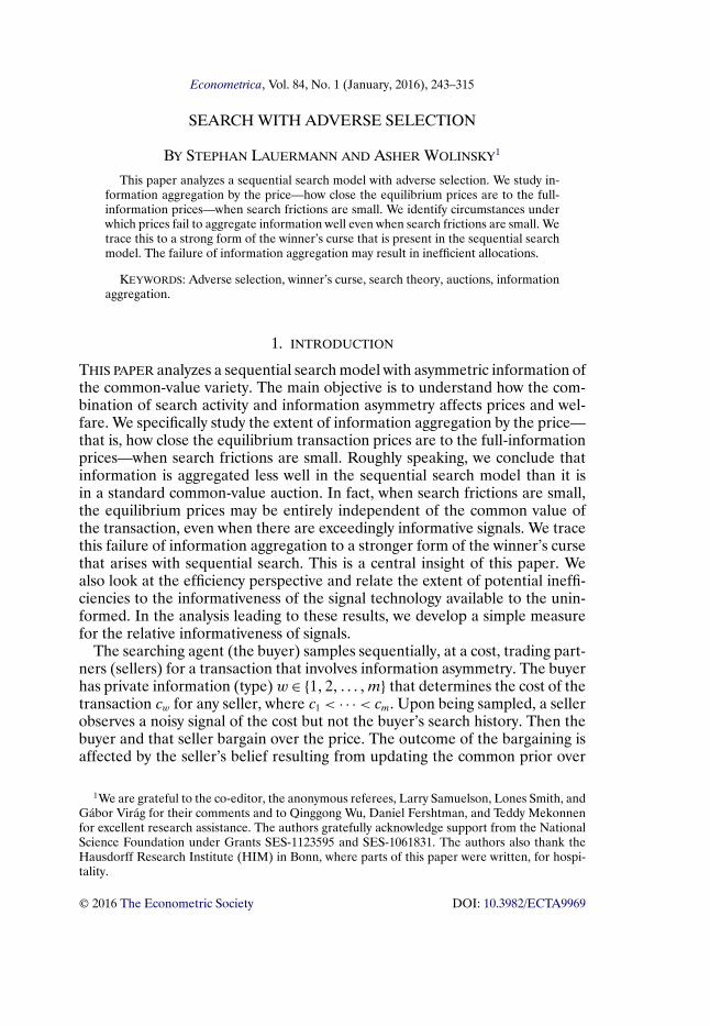
Figure 2 illustrates the acceptance strategies and the regions of mutuallyacceptable prices for an example with m = 4. In the figure, Ω1 is the set ofall signal–price pairs (x�p) such that the signal satisfies E[c|x] ≤ u − V1 andthe price p ∈ [E[c|x]�u − V1]. Since prices from this region are acceptable toall buyer types, the buyer’s acceptance decision does not contain any infor-mation. The set Ω2 = Ω1, although buyer type 2 accepts in addition all pricesp ∈ (u − V1�u − V2]. However, p ∈ (u − V1�u − V2] is only acceptable to buy-ers w ≥ 2 and, hence, the acceptance of such a price reveals w ≥ 2. But since

FIGURE 2.—Acceptance strategies and the sets (Ωi)4i=1.

14This is up to irrelevant differences concerning zero-probability events and the description ofsellers’ acceptance decisions for prices that all types of the buyer will reject.


E[c|x�w ≥ 2] > u − V2 for all x ≥ x, sellers reject all such prices. Thus, thereare no signal–price combinations that are mutually agreeable to a seller andbuyer type 2 that are not already in Ω1, that is, Ω2 \ Ω1 = ∅. The set Ω3 is theunion of the two lower shaded areas: It includes Ω1 and, in addition, all (x�p)such that E[c|x�w ≥ 3] ≤ u − V3 and p ∈ [E[c|x�w ≥ 3]�u − V3], where theconditioning reflects that these prices are only accepted by types w ≥ 3. Theset Ω3 \ Ω2 is not empty since u − V3 > E[c|x�w ≥ 3]. The set Ω4 is the unionof all three shaded areas. The set Ω4 \Ω3 consists of all (x�p) pairs such thatp ∈ [c4�u− V4]. Since acceptance of a p> u− V3 reveals that w = 4, the sellerhas nothing to learn from the signal and there is no restriction on x in Ω4 \Ω3.

The recursive structure of the sets Ωi that is evident from Figure 2 is a gen-eral implication of Lemma 2, that is,

Ω1 = {(x�p) : p ∈ [E[c|x�w ≥ 1]�u− V1

]}�(14)

Ωi+1 =Ωi ∪{(x�p) : p ∈ [E[c|x�w ≥ i+ 1]�u− Vi+1

]}�(15)

In particular, Ω1 = · · · = Ωm if Vm ≥ u−E[c|x�w ≥ 2].The system (6), (7), (11), (12), (13), (14), and (15) fully determines the

equilibrium. The sets Ωw determine the Vw’s and nw’s. The nw’s determineE[c|x�w ≥ i], which, together with the Vw’s, determine the Ωw’s. A standardfixed-point argument proves that this system has a solution and, hence, provesthe existence of an equilibrium.

PROPOSITION 1: An equilibrium exists.

The proof of this proposition in Appendix B and our later analysis utilize thatthe sets Ωw of equilibrium trades define cutoff signals ξi ∈ [x�x] as follows. IfE[c|x�w ≥ i] ≤ u−Vi ≤ E[c|x�w ≥ i], the cutoff ξi is defined to be the solutionof

u− Vi = E[c|ξi�w ≥ i]�(16)

Otherwise,

ξi ={x if u− Vi > E[c|x�w ≥ i],x if u− Vi < E[c|x�w ≥ i].

Thus, if Ωi = Ωi−1 (of course, always Ωi−1 ⊆ Ωi), the cutoff ξi is the largestsignal such that (x�p) ∈ Ωi \Ωi−1 and, if Ωi = Ωi−1, then ξi = x. Therefore,

Ωi =Ωi−1 ∪ {(x�p) : x ∈ [x�ξi]�p ∈ [E[c|x�w ≥ i]�u− Vi

]}�

with Ω0 = ∅. Figure 2 illustrates the cutoffs ξi.


3. INFORMATION AGGREGATION: FIRST STEPS

We study the extent to which information is aggregated into the equilib-rium prices when sampling costs are small. Aggregation is maximal if the pricethat each buyer type pays is equal to its cost. Aggregation is minimal whenall buyer types pay the same price. Formally, consider a sequence of samplingcosts {sk}∞

k=1 with

limk→∞

sk = 0�

and a sequence of equilibria {(Bk�Ak)}∞k=1 associated with it. The superscript

k indicates magnitudes arising in the equilibrium (Bk�Ak). Thus, we use V kw ,

Skw, nk

w, Ek, Ωkw, and so forth. Recall that Sk

w is the expected total search costincurred by type w and pk

w is the expected price. Let

pw = limk→∞

pkw and Sw = lim

k→∞Skw�

The following analysis investigates pw and Sw.To simplify the exposition, we restrict attention to sequences of equilibria

such that the prices pkw, search costs Sk

w, and the ratioΓw(Ω

kw′ )

Γw(Ωkw)

converge for alltypes w and w′ < w. Such a converging sequence can be extracted from anygiven sequence of equilibria by a compactness argument. This restriction al-lows us to avoid the introduction of multiple layers of subsequences. We donot restate it every time that limits are taken. We discuss this restriction later.We also omit the subscript k→ ∞ whenever the limit is with respect to k.

3.1. Information Aggregation With Boundedly Informative Signals

In the case of boundedly informative signals, namely,

limx→x

fi(x)

fi+1(x)<∞ for all i < m�(17)

even the most favorable signal carries only limited information. In this case,the limit equilibrium outcome as sk → 0 is shown to be complete pooling: alltypes pay the same price, which is in turn equal to the ex ante expected cost.

PROPOSITION 2: Suppose that limx→xfi(x)

fi+1(x)< ∞ for all i <m.

(i) pw = Eρ[c] for all w ∈W .(ii) Sw = 0 for all w ∈W .

The intuition behind the proof is most transparent when the set of possiblesignal values is finite, with x the lowest signal value and fw(x) > 0 its prob-ability. Suppose to the contrary that S1 > 0. Then, as we will argue, type 1


would trade with a strictly positive, nonvanishing probability every period sothat the expected search costs would vanish as sk → 0, contradicting S1 > 0.To see why type 1 would trade with a strictly positive probability, consider theset of prices Pk = [Ek[c|x]�Ek[c|x] + 1

2S1]. Since Ek[c|x] is the lowest priceany seller ever accepts, V k

1 ≤ u − Ek[c|x] − Sk1 . Hence, V k

1 < u − p′, for allp′ ∈ Pk and large k. Therefore, sequential rationality implies that type 1 ac-cepts such p′. Since p′ ≥ Ek[c|x], sellers also accept p′ after observing thesignal x. Therefore, Ωk

1 ⊇ {x} × Pk for large k. Type 1’s probability of realiz-ing signal x and a price p′ ∈ Pk is bounded away from zero. That is, for someγ > 0, Γ1({x} × Pk) ≥ γ > 0. Therefore, the probability Γ1(Ω

k1) ≥ γ > 0, as

claimed and, hence, S1 = lim sk

Γ1(Ωk1 )

≤ lim sk

γ= 0.

A similar argument establishes that p1 = limEk[c|x]. If p1 > limEk[c|x], itwould be profitable for type 1 to wait for a combination (x�p) such that pis between Ek[c|x] and p1. This is because such a combination occurs with astrictly positive, nonvanishing probability and, hence, waiting for it involves anegligible search cost as sk → 0.

It follows now from f1(x)

fw(x)< ∞ that every other type w can mimic type 1 at

no cost. This is because the MLRP implies that

sk

Γw

(Ωk

1

) = Γ1

(Ωk

1

)Γw

(Ωk

1

) sk

Γ1

(Ωk

1

) ≤ f1(x)

fw(x)

sk

Γ1

(Ωk

1

) �and together with S1 = 0 we get lim sk

Γw(Ωk1 )

≤ f1(x)

fw(x)S1 = 0.

Since every type can costlessly mimic type 1, it follows that pw = p1 =limEk[c|x]. Since all types trade after realizing signal x, it follows from thelaw of iterated expectations that limEk[c|x] =Eρ[c].

The proof presents the corresponding argument for a continuum of signals.

3.2. Proof of Proposition 2

STEP 1: For any δ > 0, there exists x(δ) > x such that for all k,

Ek[c|x(δ)]−Ek[c|x]< δ�

PROOF: Since Ek[c|x] is bounded, monotonic, and continuous, this claimfollows immediately from (10) and limx→x

fi(x)

fm(x)<∞ for all i. Q.E.D.

STEP 2:

S1 = limsk

Γ k1

(Ωk

1

) = 0�


PROOF: Suppose S1 > 0. By Step 1, there is a signal x′ = x(S1/3) > x suchthat

Ek[c|x′]−Ek[c|x]< S1/3

for all k. Since V k1 ≤ u−Ek[c|x] − 2S1/3 for all k large enough, it follows that

V k1 ≤ u−Ek[c|x′] − S1/3. Hence,

Ωk1 ⊇ [

x�x′]× [Ek[c|x′]�Ek

[c|x′]+ S1/3

]�

Therefore,

Γ k1

(Ωk

1

)≥ F(x′)(G(Ek

[c|x′]+ S1/3

)−G(Ek[c|x′]))�

Since the right-hand side stays strictly positive, lim sk

Γ k1 (Ωk

1 )= 0. Q.E.D.

STEP 3:

p1 = limEk[c|x]�PROOF: Since Ek[c|x] is increasing in x, it follows that p1 ≥ limEk[c|x].

Suppose to the contrary that p1 − limEk[c|x] = δ > 0 (for some subsequence).By Step 1, there is x′′ = x(δ

3 ) > x such that

Ek[c|x′′]−Ek[c|x]< δ

3

for all k. Define

Ωk = [x�x′′]× [

Ek[c|x′′]�Ek

[c|x′′]+ δ

3

]�

and observe that for k large enough, Ωk ⊂ Ωk1 and limΓ k

1 (Ωk) > 0. Therefore,

by the optimality of type 1’s equilibrium strategy,

V k1 ≥ u−Ek

[c|x′′]− δ

3− sk

Γ k1

(Ωk) > u−Ek[c|x] − 2δ

3− sk

Γ k1

(Ωk) �

This and Step 2 together imply

u−p1 = limV k1 ≥ u− limEk[c|x] − 2δ

3− lim

sk

Γ k1

(Ωk)

= u− limEk[c|x] − 2δ3�


where the last equality is due to lim sk

Γ k1 (Ωk)

= 0. It follows that p1 <

limEk[c|x] + δ, which contradicts the definition of δ. Q.E.D.

STEP 4:

limsk

Γw

(Ωk

1

) = 0 ∀w ∈ W

and

limE[p|(p�x) ∈Ωk

1 �w]= limEk[c|x] ∀w ∈W �

PROOF: Observe that

limsk

Γw

(Ωk

1

) = limΓ1

(Ωk

1

)Γw

(Ωk

1

) sk

Γ1

(Ωk

1

)≤ lim

f1(x)

fw(x)

sk

Γ1

(Ωk

1

) = f1(x)

fw(x)S1 = 0�

where the inequality stems from the MLRP, the next equality stems fromf1(x)

fw(x)<∞, and the final equality stems from Step 2.

Consider p such that (p�x) ∈ Ωk1 for some x. From the sellers’ optimality,

p ≥ Ek[c|x]; from the MLRP, Ek[c|x] ≥ Ek[c|x]. Finally, from the buyer’s op-timality, p ≤ u− V k

1 . Hence,

Ek[c|x] ≤ E[p|(p�x) ∈Ωk

1 �w]≤ u− V k

1 for w ∈ W �

From Steps 2 and 3, limEk[c|x] = u − limV k1 , which establishes the

claim. Q.E.D.

STEP 5:

pw = limEk[c|x] ∀w ∈W �

PROOF: Lemma 2 and Steps 2 and 3 imply that limV kw ≤ limV k

1 = u −limEk[c|x] for all w. The optimality of type w’s equilibrium strategy and Step 4imply

limV kw ≥ u− limE

[p|(p�x) ∈ Ωk

1 �w]− lim

sk

Γw

(Ωk

1

)= u− limEk[c|x]�


Thus, limV kw = u − limEk[c|x]. Now, Ωk

w ⊇ Ωk1 and Step 4 imply that Sw = 0

and, hence, limV kw = u − pw. Therefore, u − pw = u − limEk[c|x], which im-

plies the result. Q.E.D.

STEP 6:

limEk[c|x] =Eρ[c]�PROOF: Note that W k(p) = {w|(p�x) ∈ Ωk

w for some x}. From the law ofiterated expectations,

Eρ[c] =m∑i=1

ρiE[Ek[c|x�w ∈ W k(p)

]|(p�x) ∈Ωki �w = i

]�(18)

Since by Lemma 2 and the definition of Ωki , W k(p) is of the form {j� � � � �m},

for some j, the MLRP implies Ek[c|x�W k(p)] ≥ Ek[c|x�W k(p)] ≥ Ek[c|x].This and the definition of Ωk

i imply that if (p�x) ∈ Ωki , then u − V k

i ≥Ek[c|x�W k(p)] ≥ Ek[c|x]. By Steps 4 and 5, u− limV k

i = limEk[c|x]. Hence,for all i

limE[Ek[c|x�w ∈W k(p)

]|(p�x) ∈ Ωki �w = i

]= limEk[c|x]�Therefore, taking limits on (18) with respect to k → ∞ gives theresult. Q.E.D.

This concludes the proof of Proposition 2; Steps 5 and 6 establish part (i),and Step 4 and Ωk

w ⊇Ωk1 establish part (ii). Q.E.D.

An alternative argument to the law of iterated expectations from Step 6 usestwo facts about equilibrium behavior. First, when k is large enough, all typesmimic w = 1 in the sense that Ωk

1 = · · · = Ωkm. Therefore, for all w,

Ωkw = {

(x�p) : x ∈ [x�ξk1

]�p ∈ [Ek[c|x]�u− V k

1

]}�

Second, the cutoff ξk1 converges to x. These two observations together imply

that

limnk

1

nkw

= limΓw

(Ωk

1

)Γ1

(Ωk

1

) = fw(x)

f1(x)�

So the relative probability of being sampled is inversely related to the rela-tive probability of the signals: with more informative signals, the higher typessearch longer. Formally, the signal and the sampling likelihood ratio cancel,and we obtain

limηk1w

(ξk

1

)= limρ1

ρw

f1

(ξk

1

)fw(ξk

1

) nk1

nkw

= ρ1

ρw

�


In words, the posterior likelihood ratio conditional on a signal ξk1 and condi-

tional on being sampled is equal to the prior likelihood ratio. Since ξk1 con-

verges to x, it follows that when sk is small, Ek[c|x] ∼=Eρ[c] for all x ∈ [x�ξk1 ].

4. INFORMATION AGGREGATION: UNBOUNDEDLY INFORMATIVE SIGNALS

In the case of unboundedly informative signals, namely, when

limx→x

fi(x)

fi+1(x)= ∞ for all i < m�(19)

signals x→ x separate any two types.

4.1. The Informativeness Measure λij

The equilibrium behavior of type i is to search until it finds a signal–pricepair in Ωk

i . It follows from the subsequent analysis that as the sampling cost skvanishes to 0, the set of signals after which “most” trade takes place shrinks tothe bottom of the support.15 The extent to which equilibrium prices aggregateinformation will, therefore, depend on the capability of signals near x to distin-guish between the different types. Indeed, in the related auction literature (seeSection 7), the extent to which the equilibrium aggregates information is char-acterized in terms of limx→x

fi(x)

fj(x)alone. Our characterization results require a

finer measure for the case with unboundedly informative signals.For any pair of types (i� j) with i < j, let

λij = limx→x

fi(x)

fj(x)

− ln(Fi(x)

) �(20)

which may take any value in [0�∞]. This limit exists by assumption (2) andL’Hôpital’s rule. The value λij is a measure of informativeness—it is related tothe rate at which the signal’s power to distinguish type i from j improves asx → x. A larger λij means that this power increases more sharply as x → x. Iflimx→x

fi(x)

fj(x)< ∞, then λij = 0. For λij > 0, it is necessary that limx→x

fi(x)

fj(x)= ∞

but not sufficient.The measure λij plays an important role in the characterization of equilib-

rium and is an innovation of this paper. It is discussed in more detail in Sec-tion 6. We show there that for every signal distribution that is “generic,”

λij ∈ {0�∞} if i < j�(21)

15For any signal x′ > x, the probability that the buyer ends up trading with a seller observing

signal x ∈ [x′�x] goes to zero, that is, for any Ω′ = [x′�x] × [0�u], we have lim Γi(Ω′∩Ωk

i )

Γi(Ωki )

= 0. Thisis implied by Lemma 12 in Appendix C and by Propositions 4 and 5 below.


4.2. Complete Pooling and Perfect Separation

With unboundedly informative signals, it is possible to have complete pool-ing (like in the boundedly informative signals case) and it is possible to havecomplete separation. The circumstances under which either one of the possi-bilities arises are determined by the measure λij .

PROPOSITION 3:(i) If λ1�m = 0, then pw =Eρ[c] for all w.

(ii) If λw�w+1 = ∞ for all w<m, then pw = cw for all w.(iii) In both cases, Sw = 0 for all w.

The proof is at the end of Section 4.4 below. The critical role of λij owesto its relation to type j’s cost of “mimicking” type i: a larger λij means moreseparation of i from j and a larger cost of mimicking. These mimicking costsare characterized formally in Lemma 3 and an intuitive derivation is given inSection 6.

Given the results on information aggregation in large common-value auc-tions with unboundedly informative signals (which will be discussed in moredetail later), the perfect information aggregation of part (ii) is less surpris-ing than the possibility of complete pooling. Since, as mentioned above, λij isgenerically 0 or ∞, these are not necessarily knife-edge cases.

In the intermediate cases that lie between these two extremes (of λ1�m = 0and λw�w+1 = ∞ for all w < m), the picture is somewhat more complicated.This will be taken up by the next section.

4.3. The Partitional Structure of Equilibrium Outcomes

The first two results, Propositions 4 and 5, establish the partitional structureof the equilibrium in general, without using the λij measure. This structureis illustrated by Figure 1 in the Introduction. In the limit equilibrium, the setof the buyer types is partitioned into “pools” composed of adjacent types. Alltypes in each pool (except perhaps the highest type in the pool) mimic thelowest type in the pool and pay the same expected price. The highest type inthe pool does so only with some probability and may pay a higher expectedprice. The pools are separated from each other in the sense that if i < j andthey are in different pools, then in the limit, the probability that j trades at aprice near or below pi or that i trades at a price near or above pj is 0. The twoextreme cases of the previous subsection are the special cases in which there isonly one pool or all pools are singletons.

Formally, a partitional configuration is a partition (I(r))Rr=1 of W into adja-cent sets of consecutive types (“pools”), I(r) = {I(r)� I(r)+ 1� � � � � I(r)}.


Proposition 4 formalizes part of the verbal characterization of the previousparagraph. As before, Ωk

I(1)−1 = ∅.


fi+1(x)= ∞ for all i < m. Then there is a

partitional configuration (I(r))Rr=1 such that for any element I(r) = {I� � � � � I},

limΓi

(Ωk

I \ΩkI−1

)Γi

(Ωk

i

) = 1 for all i ∈ {I� � � � � I − 1}�

limΓI

(Ωk

I \ΩkI−1

)ΓI

(Ωk

I

) > 0 and

limΓI

(Ωk

I \ΩkI−1

)ΓI

(Ωk

I

) + limΓI

(Ωk

I\Ωk

I−1

)ΓI

(Ωk

I

) = 1�

The proof of this and of the following proposition are in Appendix D. Theseproofs rely on preliminary results, Lemmas 6–12 and Corollary 2, that arestated and proved in Appendix C. Roughly speaking, these preliminary resultsestablish that in the relevant cases, ξk

w → x. The main step of the proof ofthe proposition consists of showing that there are no three subsequent typesthat are “partially pooled,” in the sense that there is no i for which bothlim

Γi(Ωki−1)

Γi(Ωki )

∈ (0�1) and lim Γi+1(Ωki )

Γi+1(Ωki+1)

∈ (0�1). Intuitively, if i and i − 1 are par-

tially pooled, then it must be that Si > 0. However, if Si > 0, then ξki → x and

limx→xfi(x)

fi+1(x)= ∞ together imply that it is “infinitely” costly for type i + 1 to

mimic type i. Thus, no three types can be partially pooled, which is then shownto imply the partitional structure.

Given a partitional configuration (I(r))Rr=1 and any element I(r) = {I� � � � � I},let

α= limΓI

(Ωk

I

)ΓI

(Ωk

I

)be the probability with which the highest type in a pool, I, “mimics” the lowesttype, I, and ends up trading at some signal–price combination from Ωk

I . ByProposition 4, α > 0, and with probability (1 − α), type I ends up trading atsome signal–price combination from Ωk

I\Ωk

I−1.

Proposition 5 describes the relationship between the pools, prices, andsearch costs.



fi+1(x)= ∞ for all i < m and that

{I� � � � � I} is an element of the partition described in Proposition 4. Then

pI = · · · = pI−1 =

I−1∑i=I

ρici + αρIcI

I−1∑i=I

ρi + αρI

�

pI = αpI + (1 − α)cI

and

SI = · · · = SI−1 = 0�

SI

{= α[cI −pI] if 0 <α< 1,≤ cI −pI if α= 1.

Thus, if α= 1, then all types in the pool {I� � � � � I} pay (in the limit) the sameprice, which is equal to the expected cost conditional on the types in the pool.If 0 <α< 1, only types i ∈ {I� � � � � I−1} pay the same price (in the limit), whiletype I ends up paying the common price or a price close to its true cost cI withprobabilities α and 1 − α, respectively. This requires that near the limit, I isalmost indifferent between accepting a price p such that (x�p) ∈Ωk

I\Ωk

I (and,hence, is near cI) and incurring the expected search cost of finding (x�p) ∈ Ωk

I

to get a price near pI .Finally, a corollary of Proposition 4 gives the implication of the partitional

structure for the coefficients ηkjI(ξ

kI )= ρj

ρI

fj(ξkI )

fI (ξkI )

nkj

nkI.

COROLLARY 1: For any element {I� � � � � I} of the partition from Proposition 4,with α= limΓI(Ω

kI )/ΓI(Ω

kI),

limηkjI

(ξkI

)=

⎧⎪⎪⎪⎨⎪⎪⎪⎩

ρj

ρI

if I < j < I,

αρj

ρI

if j = I,

0 if j > I.

(22)

The proof is in Appendix D.2. Intuitively, this resembles the pooling be-havior we encountered in the case of boundedly informative signals. If j is“pooled” with I, both are trading after signal–price pairs from Ωk

I . Therefore,


nkj

nkI= ΓI (Ω

kI )

Γj(ΩkI )

≈ FI(ξkI )

Fj(ξkI )

. Hence, in the limit,nkj

nkIand

fj(ξkI )

fI (ξkI )

offset each other, implying

the result.

Multiplicity

Propositions 4 and 5 characterize the limit of sequences of equilibria forwhich pk

w, Skw, and

Γw(Ωkw′ )

Γw(Ωkw)

converge. They do not rule out the possibility thatdifferent sequences of equilibria might have different limits of this form. How-ever, since any sequence of equilibria has a subsequence along which theseobjects converge, it follows that far enough down such a sequence, each equi-librium will be near a limit configuration of the type described by Proposi-tions 4 and 5. Nevertheless, while in general we do not know whether the limitis unique, in the cases of complete pooling and complete separation consideredby Propositions 2 and 3, the limits are unique.

4.4. Using λ to Characterize the Pools

The following proposition relates the structure of the partitional configura-tion exposed by Propositions 4 and 5 to the informativeness measure λij . Itdeals with all possible values of the λij ’s without the genericity qualification.

PROPOSITION 6: Suppose {I� � � � � I} is an element of the partition described inProposition 4.

(i) λI�I < ∞.(ii) If I < i < I, then λI�i = 0.

Thus, λij = ∞ implies that i and j are in separate pools and, in thegeneric case, λII = 0. To understand the proposition better and for the sub-sequent analysis, recall that λij = lim− d

dx( fi(x)

fj(x))/ fi(x)

Fi(x)by (2) and observe that

for i < j < �,

− d

dx

(fi(x)

fj(x)

fj(x)

f�(x)

)fi(x)

Fi(x)︸︷︷︸→λi�

=− d

dx

(fi(x)

fj(x)

)fi(x)

Fi(x)︸︷︷︸→λij

fj(x)

f�(x)+

− d

dx

(fj(x)

f�(x)

)fj(x)

Fj(x)︸︷︷︸→λj�

Fi(x)

Fj(x)�(23)

It follows from (23) that if λij > 0 or λj� > 0, then λi� = ∞, since both fj(x)

f�(x)and

Fi(x)

Fj(x)diverge to ∞ as x → x. For λi� < ∞, it is necessary that λij = λj� = 0.

The proof of the proposition uses the following lemma concerning the costfor type q > I = I(r) of mimicking I by searching for (x�p) ∈ Ωk

I . The main


finding is that this mimicking cost is proportional to λIq. Recall that ηkji(x) =

ρj

ρi

fj(x)

fi(x)

nkj

nkiand that its limit is described by Corollary 1.

LEMMA 3:(i) If λ1m <∞, then

lim supsk

Γm

(Ωk

1

) ≤ λ1m(cm − c1) limm∑j=2

ηkj1

(ξk

1

)1 +

m∑i=2

ηki1

(ξk

1

) �

(ii) Suppose that {I� � � � � I} is an element of the partition described in Proposi-tion 4. If I < q ≤ I, then

lim infsk

Γq

(Ωk

I

) ≥ λIqρI(cI+1 − cI) limηk

qI

(ξkI

)1 +

I∑i=I+1

ηkiI

(ξkI

) �

(iii) If m= 2, I(1)= 2, and λ12 <∞, then

limsk

Γ2

(Ωk

1

) = λ12(c2 − c1) limηk

21

(ξk

1

)(1 +ηk

21

(ξk

1

))2 �

The proof of Lemma 3 uses V kI = u − E[p|(p�x) ∈ Ωk

I �w = I] − sk/ΓI(ΩkI )

to get

sk

Γq

(Ωk

I

) = ΓI

(Ωk

I

)Γq

(Ωk

I

)(u− V kI −E

[p|(p�x) ∈Ωk

I �w = I])�

It then evaluates the limit of the right-hand side. This is somewhat complicatedby the fact that the first term behaves roughly like

FI(ξkI )

Fq(ξkI )

and goes to infinity,while the second term goes to zero. A discussion of how and why λ enters thecharacterization in Lemma 3 is in Section 6.

PROOF OF PROPOSITION 6: Let {I� � � � � I} be an element of a limit partitionalconfiguration described by Proposition 4.

Part (i). The statement is trivial if I = I. Suppose I < I. Because V kI

≥ 0, itmust be that lim sk

ΓI (ΩkI)<∞. From Proposition 4, α= lim

ΓI (ΩkI )

ΓI (ΩkI)> 0. Therefore,

lim sk

ΓI (ΩkI)< ∞ requires lim inf sk

ΓI (ΩkI )< ∞. From Corollary 1, limηk

jI(ξkI ) exists

and limηkjI(ξ

kI ) > 0 for all I < j ≤ I. Hence, Lemma 3(ii) requires λII < ∞.


Part (ii). From part (i), λII < ∞. From (23), λII < ∞ requires that λIq = 0for all I < q < I. Q.E.D.

PROOF OF PROPOSITION 3: Part (i). If λ1m = 0, then part (i) of Lemma 3 im-plies lim sk

Γm(Ωk1 )

= 0. Since m can costlessly mimic type 1, it is intuitively obviousthat these types must be in the same pool. Formally, the payoff from mimicking1 gives a lower bound on m’s payoff

V km ≥ u−Ek

[p|(p�x) ∈ Ωk

1 �m]− sk

Γm

(Ωk

1

) �Since (p�x) ∈ Ωk

1 implies p≤ u− V k1 and limV k

1 = u−p1 by Proposition 5,

limEk[p|(p�x) ∈ Ωk

1 �m]≤ p1�

Therefore, the previous inequalities and lim sk

Γm(Ωk1 )

= 0 imply

limV km ≥ u−p1�

But by Proposition 5, this can only be true if m = I(1) and α = 1 (that is, mis pooled with 1). So, {I(1)� � � � � I(1)} = W (all types are in a single pool) andpw =Eρ[c] follows from Proposition 5.

Part (ii). Let {I� � � � � I} be any element of a limit equilibrium partition. SinceλI�I+1 = ∞ by the hypothesis, Proposition 6(i) requires that I = I. Therefore,all elements of the partition are singletons and so Proposition 5 implies pw = cwfor all w.

Part (iii). If λ1m = 0, then Sw = 0 for all w<m follows from I(1)=m (shownin the proof of part (i)) and Proposition 5, and Sm = 0 follows from α = 1 andlim sk

Γm(Ωk1 )

= 0 (also shown in the proof of part (i)).

If λw�w+1 = ∞, then Sw = 0 for all w ∈ W follows from the fact that all el-ements of the partition are singletons (shown in part (ii)) and from Proposi-tion 5. Q.E.D.

4.5. The Intermediate Case With 0 < λij <∞This section considers cases in which λij takes values in (0�∞). For interme-

diate values of λij , the outcome may involve partial pooling. We consider thecase with m= 2, for which we can provide a sharp characterization.

PROPOSITION 7: Suppose m= 2. Let λ12 = λ ∈ [0�∞].• For all 0 ≤ λ≤ ∞, S1 = 0.


• If 0 ≤ λ ≤ 1ρ2

, then

p1 = ρ1c1 + ρ2c2 and p2 = ρ1c1 + ρ2c2;S2 = λρ1ρ2(c2 − c1)�

• If 1ρ2

≤ λ ≤ ∞, then

p1 =(

1 − 1λ

)c1 + 1

λc2� and p2 = 1

λ

ρ1

ρ2c1 +

(1 − 1

λ

ρ1

ρ2

)c2;

S2 = 1λ

ρ1

ρ2(c2 − c1)�

The proposition shows that the outcome may involve complete pooling—inthe sense that both types trade at prices equal to the ex ante expected costs—even if λ > 0 and not just when λ = 0, provided that λ is not too large. Contraryto the generic case of Proposition 3, however, the expected search cost may bepositive. The ex ante expected search cost is ρ2S2. The proposition implies thatρ2S2 is small when λ is either small or large, but not for intermediate valuesof λ. It follows that welfare is not monotone in the informativeness of the signaltechnology as measured by λ: less informative signals may be associated withgreater efficiency.

5. INFORMATIVENESS AND THE EFFICIENCY OF TRADE

Because trade is always beneficial and always takes place in this model, theexpected surplus is fully determined by the expected search cost incurred bythe buyer. However, we do not have a result that ties the magnitude of suchcosts to the data of the model in all cases. For generic values of λ, we knowfrom Propositions 3 and 5 that in the two extremes of complete pooling andcomplete separation, Sw = 0 for all w and the limit equilibrium is efficient. Forthe case of m = 2, Proposition 7 completely identifies the range of λ12 underwhich positive search costs arise, but in this case the search costs are positivein the limit only for nongeneric values of λ12. More generally, we know fromProposition 5 that only the highest type in a pool might incur positive costs, butnot much more.

We now modify the basic model in a minimal way to introduce efficiencyconsiderations regarding the allocation itself. For the points made by this sub-section, it is sufficient to consider a case with two types, m = 2. Suppose thatthe model is as before, except that the buyer’s value of the transaction u nowsatisfies c1 < u< c2. Therefore, efficiency requires that type 1 trades, but type 2does not. To accommodate the possibility of no trade, there is an entry stage:the buyer decides once and for all in the beginning whether to start the search.If the search is initiated, the process continues until a transaction takes place.


The analysis of this scenario is similar to the previous analysis, except forthe buyer’s entry decision. Let e = (e1� e2) denote the probabilities with whichtypes 1 and 2 enter. A strategy profile (B�A�e) consists of the acceptancedecision of the buyer and the sellers, and the entry probabilities. A strategyprofile is an equilibrium if the standard optimality conditions hold—the onesposed above and a new one regarding the entry decision. We consider nontriv-ial equilibria in which either e1 > 0 or e2 > 0 (or both). Trivial equilibria withno entry always exist.

If entry is profitable for type 2, entry must be strictly profitable for type 1.So, in any nontrivial equilibrium, it must be that e1 = 1 when s is sufficientlysmall. Thus, the probability of type w after the decision to start the search butbefore any signals are observed is

ρ1(e2)= ρ1

ρ1 + e2ρ2and ρ2(e2) = e2ρ2

ρ1 + e2ρ2�(24)

Again, we consider a sequence sk → 0 and a corresponding sequence of non-trivial equilibria, (Bk�Ak� ek). The outcome becomes efficient if type 1 entersfor sure, its expected search cost vanishes to zero, and the entry probability oftype 2 becomes zero.

In equilibrium, trade takes place only at prices that do not exceed u and,hence, strictly below c2. Therefore, there can be no revealing transaction in-volving type 2. Consequently, if type 2 enters in equilibrium, it must be pool-ing with type 1, that is, Ωk

2 = Ωk1 for all sk. Thus, in the limit as sk → 0, the

equilibrium price must be equal to the expected cost evaluated at probabil-ities lim ρw(e

k2). That is, given these probabilities, the analysis is identical to

Proposition 7, with ρw taking the place of the original prior ρw. In particular, ifλ12 = 0, the outcome is complete pooling on the expected costs conditional onentry, ρ1c1 + ρ2c2, and ek2 stays strictly positive in the limit.16 If λ12 = ∞, thenthere is complete separation. Thus, if type 2 were to enter with strictly positiveprobability in equilibrium in the limit, its price would be close to c2. There-fore, if λ12 = ∞, it must be that ek2 → 0. The next proposition follows from theprevious arguments and its proof is therefore omitted.

PROPOSITION 8: Suppose that m = 2, c1 < u < c2, and that there is an entrystage. Consider a sequence sk → 0 and a corresponding sequence of nontrivialequilibria, {Bk�Ak� ek}. The limit equilibrium outcome is efficient if and only ifλ12 = ∞.

In the efficient outcome of this environment, only type 1 trades. This out-come is only achieved when the types are fully separated in the limit. In othercases, inefficient trade involving type 2 takes place in equilibrium.

16If ρ1c1 +ρ2c2 ≤ u, then limek2 = 1. If ρ1c1 +ρ2c2 > u, then limek2 ∈ (0�1) and ρ1c1 + ρ2c2 = uin the limit.


If λ12 = 0, the only inefficiency is excessive trade. If, however, λ12 ∈ (0�∞),then the equilibrium also involves another inefficiency: if type 2 enters, it incurssearch costs, as described in Proposition 7.

In conclusion, when trade is not always desirable, efficiency requires thatprices aggregate the information well. Complete or nearly complete poolingthat yields efficiency when all trade is desirable involves inefficient excessivetrade when not all trade is desirable.

6. MORE ABOUT λ

This section discusses further the measure λij , derives it explicitly for a spe-cific example of a family of distributions, and illustrates why it shapes the equi-librium.

Alternative Expressions

The measure λij can be expressed in a few alternative ways. Since by assump-tion the limit of (2) exists, L’Hôpital’s rule implies

λij = limx→x

− d

dx

(fi(x)

fj(x)

)fi(x)

Fi(x)

�

First, using the above equality and integration by parts,

λij = limx→x

∫ x

x

(fi(x)

fj(x)− fi(x)

fj(x)

)fi(x)

Fi(x)dx�(25)

The integral on the right-hand side captures the expected increase in fi(x)

fj(x)over

fi(x)

fj (x)resulting from a signal x ≤ x drawn from Fi.

Second, given any i and j > i, let Φij denote the c.d.f. of the ratio fifj

con-ditional on type i. It follows that Φij satisfies Φij(

fi(x)

fj(x)) = 1 − Fi(x). Hence, its

inverse hazard rate satisfies

1 −Φij

(fi(x)

fj(x)

)

φij

(fi(x)

fj(x)

) =− d

dx

(fi(x)

fj(x)

)fi(x)

Fi(x)

for all x ∈ (x�x)�

Thus,

λij = liml→∞

1 −Φij(l)

φij(l)�(26)


The equality of the right sides of (25) and (26) is an instance of a known re-sult.17 Thus, λij is the inverse hazard rate in the right tail of the distribution ofthe likelihood ratios fi

fjconditional on type i.

The expression (26) also helps one to understand why the critical bound-ary on the growth of fi

fjis − lnFi. Note that for any random variable y with

c.d.f. G, the expression y

− ln(1−G(y))behaves like the inverse hazard rate 1−G

gfor

y → ∞ (by L’Hôpital’s rule). Thus, the relative speed of growth of − ln(1 −G)determines whether the tail of the distribution of y is heavier than the tail ofan exponential distribution. Thus, the fact that the critical boundary on thegrowth of fi

fjis − lnFi is due to the fact that λij is equal to the inverse hazard

rate of the distribution of the likelihood ratios.

The Genericity Claim

Let (Fz)z∈(0�1) be a family of signal distributions. It is assumed that, for z < z′,fzfz′

is differentiable in x, limx→xfz(x)

fz′ (x)= ∞, and λzz′ exists. A finite sample of m

values of z from (0�1), 0 < z1 < · · · < zm < 1, determines an m-tuple of signaldistributions (Fz1� � � � �Fzm). Consider now an atomless distribution whose sup-port is (0�1). A sample of m independent draws from this distribution deter-mines a distribution over m-tuples of signal distributions. We say that a prop-erty is generic if the set of such samples for which it holds has probability 1.Thus, our claim about the genericity of λij ∈ {0�∞} means that for any choice ofthe family (Fz)z∈(0�1) that satisfies the above assumptions and for any atomlessdistribution on its parameter, the probability that a randomly selected finitesample of signal distributions contains a pair of signal distributions (Fzi �Fzj )for which 0 < λij <∞ is 0.

LEMMA 4: For a generic family of signal distributions,

λij ∈ {0�∞} for i < j�(27)

PROOF: From (23) and the subsequent discussion, for i < j < �,

λi� <∞ ⇒ λi�j = λj�� = 0�(28)

It follows immediately from (28) that if λzz′ ∈ (0�∞), then λzz′′ = 0 forall z′′ ∈ (z� z′), and λzz′′ = ∞ for all z′′ > z′. Therefore, for any parameterz ∈ (0�1), there is at most one parameter z+ > z such that λzz+ ∈ (0�∞) andat most one parameter z− < z such that λz−z ∈ (0�∞). This implies the re-sult. Q.E.D.

17For any random variable y with unbounded support and c.d.f. G, if limy→∞1−G(y)

g(y)= λ, then

limx→∞ E[y−x|y ≥ x] = λ. For the exponential distribution this holds away from the limit as well.


Example

Consider a family of signal distributions indexed by z ∈ (0�1] with commonsupport (−∞�−1]. Their densities are

fz(x) = (−x)−2z ex

μz

for z ∈ (0�1]�

with μz = ∫ −1−∞(−t)−2zet dt. The likelihood ratios are

fz(x)

fz′(x)= (−x)2(z′−z) μz′

μz

�

For z′ > z, limx→−∞fz(x)

fz′ (x)= ∞. These distributions also satisfy assumption (1).

Moreover, from

λz�z′ = limx→−∞

(−x)2(z′−z)−12(z′ − z

)(−x)−2zex∫ x

−∞(−t)−2zet dt

μz′

μz

�

it follows that

λz�z′ =

⎧⎪⎨⎪⎩

∞ if z′ − z > 0�5,μz′

μz

if z′ − z = 0�5,

0 if z′ − z < 0�5.

Consider now a random sample, z1 < z2 < · · · < zm, generated by an atom-less distribution on (0�1), and let (Fi)

mi=1 be the associated distributions. With

probability 1, there are no i and j in that sample such that zi − zj = 0�5, that is,λij ∈ {0�∞} for all pairs i < j. Next, let ı be the lowest i such that zi − z1 > 0�5(if such exists). Then λ1j = 0 for all j < ı, λ1ı = ∞, and λıj = 0 for all j > ı.

The Role of λ in the Characterization

Suppose m = 2. As noted after the statement of Lemma 3, type 2’s searchcosts when mimicking type 1 is

sk

Γ2

(Ωk

1

) = Γ1

(Ωk

1

)Γ2

(Ωk

1

)(Ek[c|ξk

1

]−E[p|(p�x) ∈ Ωk

1 �w = 1])�(29)


Lemma 3(iii) shows that the limit of the right-hand side of (29) is18

λ12(c2 − c1) limηk

12

(ξk

1

)(1 +ηk

12

(ξk

1

))2 �

The derivation of this expression in the proof of the lemma is quite involved. Togive some insight as to why λ appears in this characterization, let us considera similar but simpler expression. For this, note that the ratio Γ1(Ω

k1 )

Γ2(Ωk1 )

behaves

roughly like F1(ξk1 )

F2(ξk1 )

and that the expected prices closely resemble the expectedcosts of the sellers. Let us then consider

F1

(ξk

1

)F2

(ξk

1

)(Ek[c|ξk

1

]−Ek[Ek[c|x]|x≤ ξk

1 �w = 1])�(30)

Using Ek[c|x] = c2+ηk12(x)c1

1+ηk12(x)

, (30) can be written as

(c2 − c1)ρ1

ρ2

nk1

nk2

F1

(ξk

1

)F2

(ξk

1

) ∫ ξk1

x

f1(x)

f2(x)− f1

(ξk

1

)f2

(ξk

1

)(1 +ηk

12

(ξk

1

))(1 +ηk

12(x)) f1(x)

F1

(ξk

1

) dx�(31)

Using the alternative expression (25) for λ12 to rewrite the numerator, the limitof this expression over ξk

1 → x and (nk1 � n

k2)→ (∞�∞) is

(c2 − c1) limηk12

(ξk

1

) λ12(1 +ηk

12

(ξk

1

))2 �

Thus, the limits of (29) and (30) are indeed the same.Expression (31) captures the expected reduction in cost (price) that type 1

achieves by continued search after realizing signal ξk1 . Inspection of that ex-

pression reveals that this magnitude is closely related to the expected increaseof the likelihood ratio realized in such continued search. As evident from (25),λ12 exactly captures this magnitude in the limit. Intuitively, the larger is λ12, thelarger is type 1’s expected gain from continuing the search for x ≤ ξk

1 ratherthan stopping at ξk

1 . Thus, when λ12 is large, type 1 searches more (in the sensethat ξk

1 is lower), which makes it harder for type 2 to mimic type 1 and enablesseparation.

18Lemma 3 uses η21 and here we use the inverse η12. But, η12(1+η12)

2 =1

η12( 1η12

+1)2 = η21(1+η21)

2 .


7. COMPARISON TO AUCTIONS: SAMPLING CURSE VERSUS WINNER’S CURSE

The literature on auctions addresses a closely related question concerningthe extent to which the equilibrium price in a common-value auction reflectsthe information contained in the bidders’ signals when the number of biddersis made arbitrarily large (Wilson (1977) and Milgrom (1979)). In the auctionversion of our model, the buyer/auctioneer faces n sellers in a procurementauction. In state i = 1� � � � �m, each seller gets an independent signal from Fi.They submit bids simultaneously and the lowest bidder wins.

The search model of the present paper differs from the auction environmentin a number of ways: the number of “bidders” is determined endogenouslythrough the sampling, the buyer/auctioneer has private information, and thebids are generated randomly. However, the latter two are not responsible forthe differences between the results. First, as argued in Section 8 below, the bar-gaining component of the present model can be changed to let sellers submitbids without affecting the limit results. Second, since the number of biddersin the auction is not determined by the auctioneer, behavior is unaffected bythe auctioneer’s private information, and we may just as well assume that theauctioneer’s information is the same in both models.19 The important differ-ence between these two environments is that the number of sellers/bidders isexogenous in the auction environment, but is determined endogenously by theinformed buyer/auctioneer in the search environment.

The comparison is between the extent of information aggregation in the auc-tion when n→ ∞ and in the search model when s → 0. As we have seen, whensignals are boundedly informative, fi(x)

fi+1(x)< ∞, the search model exhibits com-

plete pooling. In contrast, Lauermann and Wolinsky (2013) show (for the caseof m = 2 and f1(x)

f2(x)< ∞) that the equilibrium of this auction never exhibits

complete pooling and, furthermore, that the winning bid is near the true costsif f1(x)

f2(x)and n are both large. Thus, information aggregation is more difficult in

the nearly frictionless search environment than in the large auction environ-ment. This difference between the two scenarios is explained below from theperspective of the winner’s curse.

For simplicity, the discussion will focus on m = 2 and f1(x)

f2(x)< ∞. We show

that if f1(x)

f2(x)and n are large, then the winning bid will be close to c1 with a

strictly positive probability that is bounded away from 0. That is, if ε > 0, thenfor any sufficiently large f1(x)

f2(x), it holds that

limn→∞

Pr[winning bid ≤ c1 + ε|n�w = 1] > 0�(32)

19Conversely, we may assume that the buyer has no information in our model; see the discus-sion in Section 9.


Thus, there cannot be complete pooling on some common bid b in the limit:If the winning bid were near some b with probability close to 1 in both states,then individual rationality of the bidders would require that b is above Eρ[c] =ρ1c1 + ρ2c2, contrary to (32).

To establish (32), suppose to the contrary that, for some ε > 0 and anyf1(x)

f2(x)< ∞, limn→∞ Pr[winning bid ≤ c1 + ε|n�w = 1] = 0. Now consider a bid-

der with signal x who bids just under c1 +ε. Her posterior probability of type 1conditional on winning in an auction with n bidders is

Pr[w = 1|x�win with c1 + ε]

=ρ1

ρ2

f1(x)

f2(x)

Pr[lowest bid among others ≥ c1 + ε|n�w = 1]Pr[lowest bid among others ≥ c1 + ε|n�w = 2]

1 + ρ1

ρ2

f1(x)

f2(x)

Pr[lowest bid among others ≥ c1 + ε|n�w = 1]Pr[lowest bid among others ≥ c1 + ε|n�w = 2]

�

where the ratio of the winning probabilities on the right-hand side reflectsthe winner’s curse. For large n, Pr[lowest bid among others ≥ c1 + ε|n�w] isapproximately Pr[winning bid ≥ c1 + ε|n�w]. Further, given any η > 0 andf1(x)

f2(x), select n = n(η� f1(x)

f2(x)) such that for all n > n, Pr[winning bid ≥ c1 + ε|n�

w = 1]> 1 −η, which is possible by (32). Hence, for n > n,

Pr[w = 1|x�win with c1 + ε]

≈ρ1

ρ2

f1(x)

f2(x)

Pr[winning bid ≥ c1 + ε|n�w = 1]Pr[winning bid ≥ c1 + ε|n�w = 2]

1 + ρ1

ρ2

f1(x)

f2(x)

Pr[winning bid ≥ c1 + ε|n�w = 1]Pr[winning bid ≥ c1 + ε|n�w = 2]

≥ρ1

ρ2

f1(x)

f2(x)(1 −η)

1 + ρ1

ρ2

f1(x)

f2(x)(1 −η)

�

If f1(x)

f2(x)is large enough, η is small enough, and x > x is close enough to x, then

for all n > n(η� f1(x)

f2(x)) and x≤ x,

ρ1

ρ2

f1(x)

f2(x)(1 −η)

1 + ρ1

ρ2

f1(x)

f2(x)(1 −η)

> 1 − min{ε

3�

ε

3(c2 − c1)

}�


Therefore, the expected profit of a bidder with a signal x≤ x who bids c1 +εis at least

Pr[w = 1|x�win with c1 + ε]ε+ (

1 − Pr[w = 1|x�win with c1 + ε])(c1 − c2)≥ ε

3�

When n is large, many bidders have signals in [x� x]. Hence, for some x in thisrange, the expected equilibrium profit must be smaller than ε/3, rendering theabove deviation profitable. It follows that the desired claim (32) holds.

The winner’s curse effect for a bidder who wins with c1 + ε is bounded frombelow by 1 − η. A small η means an unimportant winner’s curse effect. Theidea is that even in the worst case scenario in which this bid wins for sure whenw = 2, still very little is learned from winning and the bidder suffers almost nowinner’s curse. So the expected profit is mostly determined by x, and when xis informative, the bidder can afford to undercut.

In the search environment, the mere fact of being sampled already impliesa form of a winner’s curse. Thus, in contrast to the auction environment, anagent cannot “avoid” this curse. Formally, the posterior probability that a sellerassigns to type 1 conditional on being sampled and observing signal x is

Pr[w = 1|sampled, x] =ρ1

ρ2

f1(x)

f2(x)

n1

n2

1 + ρ1

ρ2

f1(x)

f2(x)

n1

n2

�

which reflects a “signal effect,” f1(x)

f2(x), and a “sampling effect,” n1

n2. The latter

is in some sense the counterpart of the winner’s curse effect in the auctionenvironment. However, while the signal effect may prevail over the winner’scurse effect in the auction environment, here the sampling effect n1

n2offsets the

signal effect f1(x)

f2(x). As noted, with boundedly informative signals, both types 1

and 2 search until they generate a signal–price pair (x�p) ∈ Ω1. Therefore, asargued right after the proof of Proposition 2, lim ρ1

ρ2

f1(x)

f2(x)

n1n2

= ρ1ρ2

f1(x)

f2(x)

f2(x)

f1(x)= ρ1

ρ2.

Thus, even for the lowest signal x, the sampling effect fully cancels the sig-nal effect in the search environment, whereas we have seen that in the auc-tion environment, there is no winner’s curse at x at all and the winner’scurse is bounded for signals that are sufficiently close to x. Finally, even ifsignals are unboundedly informative, the sampling effect can be overwhelm-ing: If λ12 = 0, then it follows from our main results and Corollary 1 thatlimξk1 →x

ρ1ρ2

f1(ξk1 )

f2(ξk1 )

n1n2

= ρ1ρ2

. Hence, Prk[w = 1|sampled, ξk1 ] → ρ1.

In both the search and the auction models, revelation of information re-quires signal values for which the likelihood of type 1 is high enough to offsetthe negative effect of the sampling or the winner’s curse. However, the more


substantial negative effect in the search model requires that there are signalsthat separate type 1 from type 2 even in a more pronounced way than in thelarge auction model.

In the auction model, the number of bidders is exogenous and, hence, inde-pendent of the buyer’s type. In a companion paper (Lauermann and Wolinsky(2013)), we consider an alternative auction environment in which the buyerdecides on the number of bidders at a cost and the bidders do not observe howmany others they compete against. This auction model is closer to the searchmodel in the sense that the number of bidders depends on the buyer’s type,and bidders learn some information from the mere fact of being selected. Inthe case of boundedly informative signals, when the sampling cost is negligible,that model has a partially revealing equilibrium like the auction with a largecommonly known n considered above. In addition, under some conditions, italso has a complete pooling equilibrium like the search model of the presentpaper.

8. MODELING BARGAINING

The “random proposals” bargaining protocol of this paper has been used inthe related literature, for example, Wilson (2001), Compte and Jehiel (2010),and Albrecht, Anderson, and Vroman (2010). Its main drawback is the artifi-cial character of the exogenously generated random proposals, implying thatplayers sometimes fail to realize commonly known gains from trade. The mainreason for choosing this model is that it avoids the complications of dealingwith off-path beliefs that are tangential to the main issues. In our model, thedriving forces are search frictions and adverse selection. When the search fric-tions are small, these forces determine quite tightly the range of possible agree-ments and the exact specification of the bargaining is of lesser importance. Thisis evident from the independence of our results of the exact form of the distri-bution G that generates the random proposals.

The robustness of the results is further confirmed by the fact that two alter-native bargaining protocols yield the same results.

First, in an earlier version of this paper, we modeled the bargaining com-ponent as a take-it-or-leave-it offer by the buyer. Since the buyer has privateinformation, this gives rise to multiplicity through the freedom of selecting off-path beliefs in perfect Bayesian equilibria. The equilibria that survive a certainrefinement that seems most convincing for the modeled situation20 give rise toexactly the same results as in the present version of the paper. A variation onthat model, wherein the buyer offers a direct mechanism instead of a price,which the seller accepts or rejects, also gives rise to the same results, upon

20We use the undefeated equilibrium refinement by Mailath, Okuno-Fujiwara, and Postlewaite(1993).


using the same refinement. The random proposals bargaining eliminates theneed to grapple with off-path beliefs and their refinement.

Second, we also studied a variation in which the sellers make the offers.Here, to circumvent Diamond’s paradox,21 in each period the buyer samplestwo or more sellers who observe the same signal and simultaneously offerprices. The buyer then either trades with the seller who offered the lowestprice or continues to search. Apart from the modified bargaining component,all other details of the model remain the same. Since the uninformed sellersmake the offers, out-of-equilibrium beliefs play no role and do not generatethe multiplicity noted above. Because multiple sellers sampled in each roundobserve the same signal, they play a one-shot Bertrand game, which drives theprices to the expected costs conditional on the buyer’s acceptance decision.The equilibria of this version give rise to the same results as in the presentversion. While the Bertrand version of the model shares with the random pro-posals version the advantage of not needing a refinement, the assumption con-cerning the sampling of multiple sellers in each round is perhaps less attractive.

9. DISCUSSION—VARIATIONS OF THE MODEL

This section collects remarks about possible variations and extensions of themodel.

Two-Sided Search and Matching Model

For simplicity of the exposition we chose to present the model in the lan-guage of a single searcher. However, it is straightforward to embed this modelin a two-sided search and matching model. In that version, instead of onebuyer, there is a population of buyers each of whom behaves like the buyerin our model. Upon completing their transactions, buyers exit the market. Themarket is kept in a steady state by constant flows of new buyers whose typesare distributed independently according to the prior distribution. The interimprobabilities in our model, Π(w|x), would coincide with the actual populationdistribution in the steady-state equilibrium of the matching model. The anal-ogy is complete. The matching model would not require a different analysisbut just translation of the description to the language of those models.

The assumption that the types of the entering buyers are distributed inde-pendently is important. It would make this model a two-sided search versionof Akerlof’s (1970) market in which the uncertainty pertains to each individualtransaction as opposed to uncertainty concerning a marketwide state.

21Diamond (1971) shows that the combination of sequential search and positive sampling costmay preclude equilibrium dispersion and search. In our model, if the buyer has no bargainingpower and if there is no competition between sellers, then the equilibrium price is monopolistic(equal to u), regardless of the search cost.


Observable History

The sellers’ inability to observe the buyer’s history plays a role in generat-ing the search-induced winner’s curse. Our central insight concerning com-plete pooling when signals are not informative enough would not survive inits sharp form if parts of the buyer’s search history were observable to sell-ers. Consider a scenario in which the limit equilibrium of our model involvescomplete pooling. Suppose that sellers can observe the buyer’s time on themarket but not past signals or prices. This is a natural assumption for somesituations like labor markets where the duration of unemployment might beobservable. It is straightforward to see that a complete pooling outcome can-not be an equilibrium in this case, since it would necessarily involve a longersearch for higher cost buyer types. This would imply that prices increase withtime on the market and, hence, higher cost types would end up paying higherexpected prices—even when sampling costs are small. Since a pooling outcomeis ruled out and since lower cost types always do better for the same reason theydo in our model, it must be that in any equilibrium, lower cost types pay lowerexpected prices. The actual characterization of the equilibria of this model re-quires more work and is not carried out in this paper. Nevertheless, the aboveargument establishes that, independently of the exact form of the equilibrium,it necessarily involves some separation of types, even with boundedly informa-tive signals. The fact that greater observability results in more separation is notsurprising. Intuitively, one expects that more information mitigates the adverseselection.

Obviously there are interesting environments in which the searcher’s historyis largely unobservable, as we assume, and there are other interesting environ-ments in which some of the searcher’s history is observable. The present modeldoes not cover the latter situations, whose analysis is a worthwhile direction forcontinued research.22

Buyer Does not Know Own Type

The assumption that the buyer is informed about the cost is not critical forour results. The critical assumptions are that the costs are correlated acrosssellers and that sellers observe different signals. First, in the case of boundedlyinformative signals, for sufficiently small sampling costs, we noted that the be-havior of the buyer is independent of her type, in the sense that Ωk

w is the samefor all w. In this case, for sufficiently small sk, any equilibrium in which thebuyer knows her type is also an equilibrium if the buyer does not know hertype. Second, in other cases, if the buyer observes the signals, then after a cer-tain number of encounters, the buyer could have fairly good information abouther own type. In this case, the speed of the learning is exogenous and depends

22For example, Kim (2014) and Kaya and Kim (2015) study such environments.


only on the signal technology. Therefore, when the sampling cost is small, sucha learning phase would be negligible and should not affect the results signifi-cantly. If the buyer does not observe the signals, the situation is more involved.The buyer will still be able to learn from the acceptance decision of sellersin past encounters. However, unlike the case in which the buyer directly ob-serves the signals, the effectiveness of learning is endogenously determined bythe equilibrium behavior of sellers. It is, therefore, harder to speculate on theform of the equilibrium in this case without going through the actual analysis.Nevertheless, the natural conjecture is that the sampling behavior of differenttypes would be more similar to each other if the buyer does not know her owntype, and this would make separation even more difficult

Heterogenous Valuations

This model assumes that the buyer’s valuation u is known and independentof the cost type. The introduction of heterogeneity of valuations would be aninteresting extension that may facilitate further insights into the welfare impli-cations of the failure of information aggregation. In particular, the failure ofinformation aggregation may lead to the unraveling of trade, since some typesof buyers with low costs who should trade may not find acceptable prices. Asexplained in Section 5, efficiency considerations with respect to the volume oftrade can, however, already be generated in the present model by consideringthe case of u falling inside the range of possible costs. We, therefore, did notinclude heterogeneity of the buyer’s value in addition to the buyer’s privateinformation about the sellers’ cost.

10. CONCLUSION

In a model of trade with adverse selection in a sequential search environ-ment, we studied the extent to which equilibrium prices aggregate the dis-persed information when sampling costs are small. First, with boundedly in-formative signals, prices aggregate no information. Second, with unboundedlyinformative signals, the extent of information aggregation by prices depends onthe rate at which the informativeness of signals increases in the tail of the sig-nal distribution. This rate is summarized by a simple measure λij that is definedfor every pair of types. If λ1m = 0, prices aggregate no information, even withunboundedly informative signals. If λi�i+1 = ∞ for all i < m, prices aggregatethe information perfectly.

In the corresponding auction environment with a large number of bidders,prices always aggregate some of the dispersed information, even if signals areboundedly informative. If signals are unboundedly informative, prices aggre-gate the information perfectly without additional conditions. The source ofthe difference is a stronger winner’s curse in the search model that owes to the


longer search duration of the high cost types. When the search history is unob-servable, being sampled is bad news, potentially overwhelming the informativecontent of signals entirely.

The potential failure of information aggregation may have welfare conse-quences. In a modified version of the main model in which trade is not alwaysdesirable, a failure of information aggregation translates into an inefficient al-location.

APPENDIX A: DERIVATION OF INTERIM BELIEFS

Conditioning on the realization of a signal from an atomless distribution witha continuous density is entirely standard. Therefore, if it were just the signal x,we would use Bayes formula with densities fw in the role of probabilities (asin (7)), without further comment. Updating conditional on a particular sellerbeing sampled is less standard. This is analogous to the inference problemof players in games with population uncertainty, which have been studied byMyerson (2000) and Milchtaich (2004).23 While different from each other, bothof their approaches imply (7). Myerson (2000) derives the posterior heuristi-cally by considering the limit of sampling from a large but finite number ofpotential players, in the spirit of the argument summarized by (8) in the bodyof the paper. The proof below employs Milchtaich’s (2004) approach for an al-ternative derivation that treats the uncertainty about the number of contactedsellers as a point process24 on the continuum set of sellers. Here, the condi-tional probabilities are defined through a standard consistency requirementon the expected conditional probabilities conditional on positive probabilityevents; see (33). This requirement implies, in particular, that the expected pos-terior is equal to the prior. Besides applying directly to the model (as opposedto finite approximations of the model), this approach also facilitates derivationof the conditional probabilities for the case of asymmetric sellers’ strategies.

PROOF OF LEMMA 1: Let Φ be the set of terminal histories in our model. Ev-ery terminal history ϕ ∈Φ is a sequence of the form ((w� (ji� xi�pi�α

Si �α

Bi )

ni=1);

see Section 2.1. Let Φw be the set of terminal histories with state w; F is theBorel σ-algebra of Φ.

The set J = [0�1] is the set of sellers and X = J ∪ {1� � � � �m}, with Borelσ-algebra BX . Each realization ϕ induces a simple counting measure ζ on BX

23In these games, the number of players is uncertain and the uncertainty may depend on a stateof the world. Players infer about the state of the world from being called to play. The probabilitythat any particular player is drawn is zero because the potential number of players in these gamesis unbounded.

24For an introduction to point processes and the associated definition of conditional probabil-ities, see Daley and Vere-Jones (2008, especially Sections 9.1 and 13.1) and Milchtaich (2004).


as follows. Let 1j(ϕ) = 1 if seller j is sampled in history ϕ and let 1w(ϕ) = 1 ifthe state is w. The induced counting measure of a set A ∈ BX is

ζ(A)=∑j∈A

1j(ϕ)+∑w∈A

1w(ϕ)�

Let N be the set of all simple counting measures on BX and let BN be theBorel σ-algebra on N .

Fix any strategy profile (B�A). This strategy profile and the chance moves(buyer’s type, signal realizations, and price proposals) induce a probabilitymeasure μ on Φ�F . The probability space (Φ�F�μ), in turn, defines a proba-bility measure—a point process—P on BN . Let Uw = {ζ ∈ N |ζ(w) = 1} ∈ BN ,the event that the state is w. We are interested in

Πj(w) = Pr[Uw|ζ(j)= 1

]�

the probability of w conditional on j being sampled. In the theory of pointprocesses, Π(·)(w) is referred to as a Palm probability; see Daley and Vere-Jones(2008, Chapter 13). The conditional probability Π(·)(w) is almost everywhereuniquely defined by the requirement∫

Φ

( ∑j∈J|1j (ϕ)=1

Πj(w)

)μ(dϕ)=

∫Φ

( ∑j∈J|1j (ϕ)=1

1w(ϕ)

)μ(dϕ) ∀J ∈ BX ;(33)

see Proposition 13.1.IV in Daley and Vere-Jones (2008). Q.E.D.

LEMMA 5: If Π(·)(w) satisfies (33), then

Πj(w) = ρwnw∑i∈W

ρini

a.e. j ∈ [0�1]�

PROOF: First, suppose the seller’s acceptance strategies are symmetric tosimplify exposition. The (Lebesgue) measure of a set J ∈ BX is λ(J) = ∫

Jdj.

Rewriting the right-hand side of (33) gives∫Φ

( ∑j∈J|1j (ϕ)=1

1w(ϕ)

)μ(dϕ) =

∫Φw

∣∣{j ∈ J : 1j(ϕ)= 1}∣∣μ(dϕ)

= ρwE[n(ϕ)|ϕ ∈Φw

]λ(J)

= ρwnwλ(J)�

Thus, the right-hand side of (33) depends on J only through its measure λ(J).Therefore, Πj(w) must be constant for almost all j. Denote this constant


by Π(w). Suppose λ(J) > 0 and rewrite (33) further:

Π(w)

∫Φ

∣∣{j ∈ J : 1j(ϕ) = 1}∣∣μ(dϕ)= ρwnwλ(J) ⇔

Π(w)∑i∈W

ρiniλ(J) = ρwnwλ(J) ⇔

Π(w) = ρwnw∑i∈{1��m}

ρini

�

Asymmetric Acceptance Strategies. For any nonzero set of sellers, we define

qw(J) = 1λ(J)

∫ ∫ ∫{(j�x�p):j∈J�p∈Aj(x)�p∈Bw

}g(p)fw(x)dpdxdj�

the probability to trade conditional on sampling a seller j ∈ J and state w.For ε > 0, let Jε be any set with Lebesgue measure λ(Jε) = ε. Abbrevi-ate qε

w = qw(Jε) and q¬εw = qw([0�1] \ Jε), and define qw = limε→0 q

εw, q¬

w =limε→0 q

¬εw .

Condition (33) holds for all Jε. We multiply both sides by 1/λ(Jε) and takethe limit as ε → 0. The limit of the right-hand side of (33)

λ(Jε)is

limε→0

1λ(Jε)

∫Φ

( ∑j∈Jε|1j (ϕ)=1

1w(ϕ)

)μ(dϕ)

= limε→0

(ρwq

εw + ρw

λ(Jε)

∞∑n=2

n∑k=1

k

(n− 1k− 1

)λ(Jε)q

εw

[λ(Jε)

(1 − qε

w

)]k−1

× [(1 − λ(Jε)

)(1 − q¬ε

w

)]n−k

+ ρw

λ(Jε)

∞∑n=2

n∑k=1

k

(n− 1k

)q¬εw

(1 − λ(Jε)

)[λ(Jε)

(1 − qε

w

)]k

× [(1 − λ(Jε)

)(1 − q¬ε

w

)]n−k−1

)

= ρw

( ∞∑n=0

qw

(1 − q¬

w

)n −∞∑n=1

qwq¬w

(1 − q¬

w

)n−1n+ nw

)

= ρw

(qw

q¬w

− qw

q¬w

+ nw

)= ρwnw�


Following the first equality, n counts the total number of contacted sellers andk counts those from Jε. The first two terms correspond to histories that endwith the buyer trading with a seller from Jε and the third term correspondsto those that do not. The second equality follows from the fact that all termsinvolving k≥ 2 converge to zero.

Take any number Π such that there is a sequence {Jεk}∞k=1 such that λ(Jεk)=

εk > 0, limk→∞ εk = 0, and |Πj(w) − Π| ≤ 1k

for all j ∈ Jεk (there is a positivemeasure of sellers with posteriors close to Π). Using the previous evaluationof the limit of the right-hand side of (33), limε→0

(33)λ(Jε)

becomes

Π limk→∞

1λ(Jεk)

∫Φ

∣∣{j ∈ Jεk |1j(ϕ)= 1}∣∣μ(dϕ)= ρwnw�

Rewriting the left-hand side of (33) analogous to the previous rewriting gives

limk→∞

Π1

λ(Jεk)

∫Φ

∣∣{j ∈ Jεk |1j(ϕ) = 1}∣∣μ(dϕ)= Π

∑i∈W

ρini�

Together,

Π = ρwnw∑i∈W

ρini

�

Thus, Πj is uniquely determined as claimed for almost every j. Q.E.D.

A similar argument establishes

Πj(w|x)= ρwfw(x)nw∑i∈W

ρifi(x)ni

for almost all j and x. The derivation of the posterior conditional on a sig-nal realization x ∈ [x�x] is entirely conventional, however, and so we omit itsdetailed derivation.

APPENDIX B: EQUILIBRIUM STRATEGIES, PAYOFFS AND EXISTENCE

RESTATEMENT OF LEMMA 2: In every equilibrium:(i) Vw is strictly decreasing in w.

(ii) Acceptance strategies are given by

Bw = [0�u− Vw]�

A(x) =m⋃i=1

[E[c|x�w ≥ i]�u− Vi

]�


PROOF OF LEMMA 2: We have already established that the equilibriumstrategies are for the buyer Bw = [0�u− Vw] and for the seller A(x) = {p|p ≥E[c|x�W (p)]}, where W (p)= {w|p ∈ Bw}. So

A(x) =m⋃i=1

[E[c|x� {w|Vw ≤ Vi}

]�u− Vi

]�(34)

To verify part (i), suppose that Vw is strictly decreasing for w ≤ j− 1 and thatVj−1 > Vw for all w > j − 1. (This includes the case of j = 1 by letting V0 = u.)Let i = arg maxw>j−1 Vw, which may or may not be equal to j. It follows from(34) and Bw = [0�u− Vw] that

Ωi ={(x�p)

∣∣∣p ∈j−1⋃�=1

[E[c|x�w ≥ �]�u− V�

]

∪ [E[c|x�w ≥ j]�u− Vi

]}�

Since E[c|x�w ≥ �] and fi(x)

fj(x)are increasing in x, we have E(x�p)[p|(x�p) ∈

Ωi�w = j] ≤ E(x�p)[p|(x�p) ∈ Ωi�w = i] and Γj(Ωi) ≥ Γi(Ωi), where the in-equalities are strict if i = j. Using (13), it follows that

Vi = u−E(x�p)

[p|(x�p) ∈Ωi�w = i

]− s

Γi(Ωi)

≤ u−E(x�p)

[p|(x�p) ∈Ωi�w = j

]− s

Γj(Ωi)≤ Vj�

where the first inequality follows from the previous inequalities in the text andthe second inequality follows from the possible suboptimality for buyer type jof mimicking type i. The first inequality is strict if i = j. Thus, i = j and Vj > Vw

for all w> j.Part (ii) follows from (34) and the monotonicity of Vw. Q.E.D.

Two Useful Observations for Use in Subsequent Proofs

Using the cutoffs {ξj}mj=1 and (14), the trading probability of type i whenfollowing type �’s acceptance strategy is

Γi(Ω�) =�∑

j=1

∫ ξj

x

(G(u− Vj)(35)

−G(max

{E[c|x�w ≥ j]�u− Vj−1

}))fi(x)dx�


with V0 = u and noting that the definition of ξj implies that u − Vj ≥E[c|x�w ≥ j] for x < ξj . Using the definition of the ξj ’s and (35) to rewriteSi = s

Γi(Ωi), the expected payoff equation, Vi = u−pi − Si, can be written as

s =i∑

j=1

∫ ξj

x

(∫ u−Vj

max{E[c|x�w≥j]�u−Vj−1}(u− Vi −p)g(p)dp

)fi(x)dx�(36)

PROOF OF PROPOSITION 1 (AN EQUILIBRIUM EXISTS): Let N =[1� us]m. We

define a mapping from N to itself whose fixed point is the equilibrium numberof expected searches for each type. Given n ∈N , let

E[c|x�n�w ≥ j] =cm +

m−1∑i=j

ρi

ρm

fi(x)

fm(x)

ni

nm

ci

1 +m−1∑i=j

ρi

ρm

fi(x)

fm(x)

ni

nm

�

Given n, payoffs {Vi(n)}mi=1 are defined iteratively as solutions to (36). Thatis, letting ξi(n�Vi) = inf{x ∈ [x�x]|E[c|x�n�w ≥ i] ≥ u − Vi}, where inf∅ = xand V0 = u, the {Vi(n)}mi=1 are the Vi’s that satisfy

s =i∑

j=1

∫ ξj(n�Vj)

x

(∫ u−Vj

max{E[c|x�n�w≥j]�u−Vj−1}(u− Vi −p)g(p)dp

)fi(x)dx�

Inspection reveals that a unique solution {Vi(n)}mi=1 exists and is continuousin n. For example, for i = 1,

s =∫ ξ1(n�V1)

x

(∫ u−V1

E[c|x�n�w≥1](u− V1 −p)g(p)dp

)f1(x)dx�

Existence, uniqueness, and continuity of V1(n) in n follow because the right-hand side is continuous and strictly decreasing in V1, and because it is strictlysmaller than the left-hand side when V1 = u (it is zero, since then ξi = x) and isstrictly larger than the left-hand side if V1 = 0 (by Assumption (3)). Analogousarguments establish the claim for i > 1.

The payoffs {Vi(n)}mi=1 and costs E[c|x�n�w ≥ i] define {Ωi(n)}mi=1 iteratively,via (14) and (15), that is,

Ωi(n) = Ωi−1(n)

∪ {(x�p) : x ∈ [x�ξi]�p ∈ [E[c|x�n�w ≥ i]�u− Vi(n)]}�


with Ω0 = ∅. Again, {Ωi(n)}mi=1 are uniquely defined and Γi(Ωi(n)) is continu-ous in n. Finally, let

ni(n)= 1Γi

(Ωi(n)

) �The function n(n) maps N into itself. In particular, ni(n) ≤ u

sfor all i. To

see why, suppose that ni(n) > us. This implies Vi(n) < 0 by (36). Then [x�x] ×

[cm�u] ⊂ Ωi(n). Hence, ni(n) ≤ 11−G(cm)

. Assumption (3) implies, in particular,that s

1−G(cm)≤ u. Hence, ni(n)≤ u

s, in contradiction to ni(n) > u

s.

Since the set N is convex and compact, and n is a continuous function map-ping N into itself, n has a fixed point. The values of Vw and Ωw that corre-spond to this fixed points through the above construction constitute an equi-librium. Q.E.D.

APPENDIX C: INTERMEDIATE RESULTS FOR THE CHARACTERIZATION

This appendix contains intermediate developments and results that do notappear in the body of the paper, but that are needed for the proofs of the mainresults in Appendix D below. We assume limx→x

fi(x)

fi+1(x)= ∞ throughout this

appendix.Recall that we consider a sequence of equilibria along which pk

w, Skw, and

Γw(Ωkw′ )

Γw(Ωkw)

converge for all w and w′ < w. Of course, the expected payoffs thenalso converge, with limV k

w = u− limpkw − limSk

w.

LEMMA 6: Preliminaries.(i) If Ωk

q =Ωkq−1 for all k large, then limV k

q ≥ u− lim infEk[c|ξkq�w ≥ q].

(ii) If Ωkq =Ωk

q−1 for all k large, then limV kq = u− limEk[c|ξk

q�w ≥ q].(iii) If Ωk

q = Ωkq−1 for all k large, then Sq > 0 if and only if limEk[p|(p�x) ∈

Ωkq�q] < limEk[c|ξk

q�w ≥ q].

PROOF: Parts (i) and (ii). If ξkq < x for all k large for some (sub)sequence,

then these statements follow from the definition of ξkq .

Suppose ξkq = x for all k large. This implies V k

q ≤ u − Ek[c|x�w ≥ q]. But,for any ε > 0, for sk small enough, type q incurs less than ε search costs bywaiting for a price p ∈ [Ek[c|x�w ≥ q]�Ek[c|x�w ≥ q] + ε] (accompanied byany x). Therefore, V k

q ≥ u− (Ek[c|x�w ≥ q] + ε)− ε, implying the results.Part (iii) follows from

u− limEk[c|ξk

q�w ≥ q]= limV k

q

= u− limEk[p|(p�x) ∈Ωk

q�q]− Sq�


where the first equality is from part (ii) of the lemma and the second equalityis from the definition of V k

q . Q.E.D.

LEMMA 7: If Ωkq =Ωk

q−1 for all k large, then for all j ≥ q,

lim(E[p|(p�x) ∈ Ωk

q \Ωkq−1� j

]−Ek[c|ξk

q�w ≥ q])= 0�(37)

PROOF: It is sufficient to prove the lemma for (sub)sequences for which thetwo terms in (37) converge. Suppose that (37) fails for some q and j ≥ q.By the definition of Ωk

q and Lemma 6, we have E[p|(p�x) ∈ Ωkq \ Ωk

q−1� j] ≤Ek[c|ξk

q�w ≥ q]. Therefore, (37) failing to hold means that, for some j ≥ q,

limE[p|(p�x) ∈Ωk

q \Ωkq−1� j

]< limEk

[c|ξk

q�w ≥ q]�(38)

STEP 1: lim sup nkinkq

<∞ for all i > q.

PROOF: By MLRP, (38) must hold for j = q as well. Hence, from Lemma 6,Sq > 0. If, in contrast to the claim, lim nki

nkq= ∞ for some i > q, then

limSki = lim sknk

q

nki

nkq

= Sq limnki

nkq

= ∞�

This contradicts the optimality of i’s behavior. Q.E.D.

STEP 2:

limEk[c|ξk

q�w ≥ q]= cq�(39)

PROOF: Recall that

Ek[c|x�w ≥ q] =cq +

m∑i=q+1

ηkiq(x)ci

1 +m∑

i=q+1

ηkiq(x)

� where ηkiq(x) = ρi

ρq

nki

nkq

fi(x)

fq(x)�

Therefore, limx→xfi(x)

fq(x)= 0 and lim sup nki

nkq< ∞ (from Step 1) for all i > q imply

that for any ε > 0, there exists xε > x such that for all k,

cq ≤Ek[c|x�w ≥ q] ≤ cq + ε for x ∈ [x�xε]�(40)


Thus, if limξkq = x for any (sub)sequence, then (39) follows immediately. If

limξkq = x > x for any (sub)sequence, then u− V k

q ≥Ek[c|ξkq�w ≥ q] and from

(36),

sk ≥∫ ξkq

x

(∫ u−V kq

Ek[c|x�w≥q]

(u− V k

q −p)g(p)dp

)fq(x)dx

≥∫ ξkq

x

(∫ Ek[c|ξkq �w≥q])

Ek[c|x�w≥q]

(Ek[c|ξk

q�w ≥ q]−p

)g(p)dp

)fq(x)dx�

Hence, for every x ∈ (x� x), sk → 0 implies

limEk[c|x�w ≥ q] = limEk[c|ξk

q�w ≥ q]�(41)

and, in particular, for x = xε for any ε > 0. It therefore follows from (40) that(39) holds in this case as well.

Thus, (39) holds, since there exists a subsequence for which limξkq exists

and for this subsequence either limξkq > x or limξk

q = x. We have shown thatin either case, limEk[c|ξk

q�w ≥ q] = cq holds. This suffices given our startingassumption that limEk[c|ξk

q�w ≥ q] exists. Q.E.D.

Now,

lim infE[p|(p�x) ∈Ωk

q \Ωkq−1�w = q

]≥ cq = limEk[c|ξk

q�w ≥ q]�(42)

where the inequality follows from the fact that (p�x) ∈ Ωkq \Ωk

q−1 implies p ≥ cqand the equality follows from Step 2. But, (42) contradicts (38). Therefore, (37)must hold for all q and j ≥ q. This proves Lemma 7. Q.E.D.

LEMMA 8: If Ωkq =Ωk

q−1 for all k large, then

lim

⎛⎜⎜⎜⎜⎜⎝Ek

[c|ξk

q�w ≥ q]−

m∑i=q

ρi

Γi

(Ωk

q \Ωkq−1

)Γi

(Ωk

i

) ci

m∑i=q

ρi

Γi

(Ωk

q \Ωkq−1

)Γi

(Ωk

i

)

⎞⎟⎟⎟⎟⎟⎠= 0�


PROOF: It is sufficient to prove the lemma for (sub)sequences for whichlimEk[c|ξk

q�w ≥ q] exists. From the law of iterated expectations,

m∑i=q

ρi

Γi

(Ωk

q \Ωkq−1

)Γi

(Ωk

i

) E[E[c|x�w ≥ q]|(p�x) ∈ Ωk

q \Ωkq−1� i

]m∑i=q

ρi

Γi

(Ωk

q \Ωkq−1

)Γi

(Ωk

i

)(43)

=

m∑i=q

ρi

Γi

(Ωk

q \Ωkq−1

)Γi

(Ωk

i

) ci

m∑i=q

ρi

Γi

(Ωk

q \Ωkq−1

)Γi

(Ωk

i

) �

For all x ≤ ξkq , the MLRP implies that Ek[c|x�w ≥ q] ≤ Ek[c|ξk

q�w ≥ q].Hence, for any i ≥ q,

E[Ek[c|x�w ≥ q]|(p�x) ∈ Ωk

q \Ωkq−1� i

]≤Ek[c|ξk

q�w ≥ q]�(44)

This inequality must not be strict in the limit. If the limit were strict, itwould imply limE[p|(p�x) ∈ Ωk

q \ Ωkq−1� i] < limEk[c|ξk

q�w ≥ q], contradict-ing Lemma 7. So, for all i ≥ q,

limE[Ek[c|x�w ≥ q]|(p�x) ∈Ωk

q \Ωkq−1� i

]= limEk[c|ξk

q�w ≥ q]�

Thus, taking limits on (43) implies the claim. Q.E.D.

Lemma 9 below uses Lemmas 7 and 8 to provide an alternative expressionfor limηk

jq(ξkq). Its proof (and some subsequent proofs) use the following claim.

CLAIM 1: For any (αi�βi� ci)ni=1 ≥ 0 such that

∑n

i=1 αi > 0, 0 <β1 < · · · <βn,and 0 < c1 < · · ·< cn,

n∑i=1

αiβici

n∑i=1

αiβi

≥

n∑i=1

αici

n∑i=1

αi

�

and the inequality is strict if there are two or more positive αi’s.

PROOF: The terms αiβi/(∑n

i=1 αiβi) and αi/(∑n

i=1 αi) define measures on ithat are ordered by first-order stochastic dominance. The claim follows frommonotonicity of ci in i. Q.E.D.


LEMMA 9: If limΓq(Ω

kq\Ωk

q−1)

Γq(Ωkq)

> 0, then for all j > q,

lim

⎛⎜⎜⎜⎜⎝ηk

jq

(ξkq

)− ρj

ρq

Γj

(Ωk

q \Ωkq−1

)Γj

(Ωk

j

)Γq

(Ωk

q \Ωkq−1

)Γq

(Ωk

q

)

⎞⎟⎟⎟⎟⎠= 0�(45)

PROOF: It is sufficient to prove the lemma for (sub)sequences for which thetwo terms in (45) and Ek[c|ξk

q�w ≥ q] converge. From Lemma 8,

lim

cq +m∑

i=q+1

ρi

ρq

nki

nkq

fi(ξkq

)fq(ξkq

)ci1 +

m∑i=q+1

ρi

ρq

nki

nkq

fi(ξkq

)fq(ξkq

)(46)

= lim

cq +m∑

i=q+1

ρi

ρq

Γi

(Ωk

q \Ωkq−1

)/Γi

(Ωk

i

)Γq

(Ωk

q \Ωkq−1

)/Γq

(Ωk

q

)ci1 +

m∑i=q+1

ρi

ρq

Γi

(Ωk

q \Ωkq−1

)/Γi

(Ωk

i

)Γq

(Ωk

q \Ωkq−1

)/Γq

(Ωk

q

) �

where the left-hand side is limEk[c|ξkq�w ≥ q] and the right-hand side is ob-

tained by dividing through byΓq(Ω

kq\Ωk

q−1)

Γq(Ωkq)

the second term in the statement ofLemma 8.

For j > � > q, we obtain that

Γ�

(Ωk

q \Ωkq−1

)Γq

(Ωk

q \Ωkq−1

)Γj

(Ωk

q \Ωkq−1

)Γq

(Ωk

q \Ωkq−1

) = Γ�

(Ωk

q \Ωkq−1

)Γj

(Ωk

q \Ωkq−1

) ≥ F�

(ξkq

)Fj

(ξkq

) ≥ f�(ξkq

)fj(ξkq

) =

f�(ξkq

)fq(ξkq

)fj(ξkq

)fq(ξkq

) �

Hence, we conclude that

fj(ξkq

)fq(ξkq

)Γj

(Ωk

q \Ωkq−1

)Γq

(Ωk

q \Ωkq−1

) ≥

f�(ξkq

)fq(ξkq

)Γ�

(Ωk

q \Ωkq−1

)Γq

(Ωk

q \Ωkq−1

) �(47)


From nki = 1/Γi(Ω

ki ), it follows that

ρi

ρq

nki

nkq

fi(ξkq

)fq(ξkq

) = ρi

ρq

Γi

(Ωk

q \Ωkq−1

)Γi

(Ωk

i

)Γq

(Ωk

q \Ωkq−1

)Γq

(Ωk

q

)fi(ξkq

)fq(ξkq

)Γi

(Ωk

q \Ωkq−1

)Γq

(Ωk

q \Ωkq−1

) �

Thus, Claim 1 implies that (46) holds only if equality holds coefficient by coef-ficient. Q.E.D.

LEMMA 10: Suppose for some i, lim Γj(Ωki )

Γj(Ωkj )

= 0 for all j > i. Then limV ki ≥

u− ci.

PROOF: Let i′ be the highest type such that i′ ≤ i and limΓi(Ω

ki′ \Ωk

i′−1)

Γi(Ωki )

> 0.

Since lim Γj(Ωki )

Γj(Ωkj )

= 0 for all j > i, we also have limΓj(Ω

ki′ )

Γj(Ωkj )

= 0 for all j > i.

This observation, together with limΓi(Ω

ki′ \Ωk

i′−1)

Γi(Ωki )

> 0 and Lemma 9 implies that

limEk[c|ξki′�w ≥ i] = ci.

From the choice of i′, it follows that ξki′ > x. If limEk[c|ξk

i′�w ≥ i] <limu− V k

i , then i′ < i and

limΓi

(Ωk

i \Ωki′)

Γi

(Ωk

i′ \Ωki′−1

) ≥ limΓi

([x�ξk

i′]× [

Ek[c|ξk

i′�w ≥ i]�u− V k

i

])Γi

([x�ξk

i′]× [

0�Ek[c|ξk

i′�w ≥ i]]) > 0�

where the first inequality owes to Ωki′ \ Ωk

i′−1 ⊂ [x�ξki′ ] × [0�Ek[c|ξk

i′�w ≥ i]]and [x�ξk

i′ ] × [Ek[c|ξki′�w ≥ i]�u − V k

i ] ⊂ Ωki \ Ωk

i′ , and the second is ob-vious from the arguments of Γi on the numerator and denominator be-ing rectangles with common base. But this is a contradiction, since fromthe choice of i′, it follows that lim

Γi(Ωki \Ωk

i′ )Γi(Ω

ki )

= 0 andΓi(Ω

ki′ \Ωk

i′−1)

Γi(Ωki )

> 0, and, hence,

limΓi(Ω

ki \Ωk

i′ )Γi(Ω

ki′ \Ωk

i′−1)= 0. Q.E.D.

LEMMA 11:(i) If lim

Γi(Ωki−1)

Γi(Ωki )

= 0, then for all j,

Γj

(Ωk

i

)= Δk

i +∫ ξki

x

g(pk(x)

)(Ek[c|ξk

i �w ≥ i]−Ek[c|x�w ≥ i])fj(x)dx

+ Γj

(Ωk

i−1

)


for all sufficiently large k, where

pk(x) ∈ [Ek[c|x�w ≥ i]�Ek[c|ξk

i �w ≥ i]]�

Δki = max

{G(u− V k

i

)−G(Ek[c|x�w ≥ i])�0

}�

(ii) ∫ ξki

x

(Ek[c|ξk

i �w ≥ i]−Ek[c|x�w ≥ i])fq(x)dx

=∫ ξki

x

(d

dxEk[c|x�w ≥ i]

)Fq(x)dx

=∫ ξki

x

m∑j=i+1

ηkji(x)

m∑z=i+1

ηkzi(x)+ 1

bki (x)

(−

d

dx

(fi(x)

fj(x)

)fi(x)

Fi(x)

)Fq(x)

Fi(x)fj(x)dx�

where bkm(x) = 0 and for i <m,

bki (x) =

m∑j=i+1

dηkji(x)

dxcj

m∑j=i+1

dηkji(x)

dx

−ci +

m∑j=i+1

ηkji(x)cj

1 +m∑

j=i+1

ηkji(x)

�(48)

(iii) For i < m, the function bki satisfies

cm − ci > bki (x)≥ ci+1 − ci

1 +m∑

j=i+1

ηkji(x)

> 0�(49)

PROOF: Part (i). It follows from (35) that

Γj

(Ωk

i

)=∫ ξki

x

(G(u− V k

i

)−G

(max

{Ek[c|x�w ≥ i]�u− V k

i−1

}))dFj(x)+ Γj

(Ωk

i−1

)= Δk

i +∫ ξki

x

(G(Ek[c|ξk

i �w ≥ i])

−G(max

{Ek[c|x�w ≥ i]�u− V k

i−1

}))dFj(x)+ Γj

(Ωk

i−1

)�


From Lemma 10 and limΓj′ (Ωk

i−1)

Γj′ (Ωkj′ )

= 0 for all j′ ≥ i, limu − V ki−1 ≤ ci−1 implies

that max{Ek[c|x�w ≥ i]�u − V ki−1} = Ek[c|x�w ≥ i] for large k. Now, part (i)

follows from the mean value theorem.Part (ii). Using integration by parts,∫ ξki

x

(Ek[c|ξk

i �w ≥ i]−Ek[c|x�w ≥ i])fq(x)dx(50)

= [(Ek[c|ξk

i �w ≥ i]−Ek[c|x�w ≥ i])Fq(x)

]ξkix

−∫ ξki

x

(− d

dxEk[c|x�w ≥ i]

)Fq(x)dx

=∫ ξki

x

(d

dxEk[c|x�w ≥ i]

)Fq(x)dx�

Recalling that Ek[c|x�w ≥ i] = ci+∑m

j=2 ηkji(x)cj

1+∑mj=2 η

kji(x)

and ηkji(x)= ρj

ρi

nkj

nki

fj(x)

fi(x),

dEk[c|x�w ≥ i]dx

(51)

=

m∑j=i+1

dηkji(x)

dx

m∑j=i+1

ηkji(x)+ 1

⎛⎜⎜⎜⎜⎜⎝

m∑j=i+1

dηkji(x)

dxcj

m∑j=i+1

dηkji(x)

dx

−ci +

m∑j=i+1

ηkji(x)cj

1 +m∑

j=i+1

ηkji(x)

⎞⎟⎟⎟⎟⎟⎠

=m∑

j=i+1

ηkji(x)

m∑j=i+1

ηkji(x)+ 1

⎛⎜⎜⎝−

d

dx

(fi(x)

fj(x)

)fi(x)

Fi(x)

⎞⎟⎟⎠ fj(x)

Fi(x)bki (x)�

where the second equality uses the definition of bki (x) and where d

dxηk

ji(x) isrewritten as

ρj

ρi

nkj

nki

d

dx

(fj(x)

fi(x)

)= ρj

ρi

nkj

nki

(−1)d

dx

(fi(x)

fj(x)

)(fi(x)

fj(x)

)−2

= ηkji(x)(−1)

d

dx

(fi(x)

fj(x)

)fj(x)

fi(x)�

Plugging (51) into (50) yields the claim in part (ii).


Part (iii). Differentiating fj(x)

fi(x)= fj(x)

f�(x)

f�(x)

fi(x)and dividing both sides by fj(x)

fi(x)yields

d

dx

(fj(x)

fi(x)

)fj(x)

fi(x)

=d

dx

(fj(x)

f�(x)

)fj(x)

f�(x)

+d

dx

(f�(x)

fi(x)

)f�(x)

fi(x)

�

Therefore, for j > � > i,

d

dx

(fj(x)

fi(x)

)fj(x)

fi(x)

>

d

dx

(f�(x)

fi(x)

)f�(x)

fi(x)

�(52)

Since

dηkji(x)

dx= ρj

ρi

nkj

nki

d

dx

(fj(x)

fi(x)

)

= ρj

ρi

nkj

nki

fj(x)

fi(x)

d

dx

(fj(x)

fi(x)

)(fj(x)

fi(x)

) = ηkji

d

dx

(fj(x)

fi(x)

)(fj(x)

fi(x)

) �

it follows from Claim 1 and (52) that, for any k,m∑

j=i+1

dηkji(x)

dxcj

m∑j=i+1

dηkji(x)

dx

≥

m∑j=i+1

ηkji(x)cj

m∑j=i+1

ηkji(x)

�

Therefore,

bki (x) ≥

m∑j=i+1

ηkji(x)cj

m∑j=i+1

ηkji(x)

−ci +

m∑j=i+1

ηkji(x)cj

1 +m∑

j=i+1

ηkji(x)

= 1

1 +m∑

j=i+1

ηkji(x)

⎛⎜⎜⎜⎜⎜⎝

m∑j=i+1

ηkji(x)cj

m∑j=i+1

ηkji(x)

− ci

⎞⎟⎟⎟⎟⎟⎠ �


which implies (49) immediately. Q.E.D.

LEMMA 12: For all i < m, if lim Γi+1(Ωki )

Γi+1(Ωki+1)

> 0 or limΓi(Ω

ki−1)

Γi(Ωki )

= 0, then

limξki = x�

PROOF:

STEP 1: Suppose limξki = x > x. Then

limEk[c|x�w ≥ i] = limEk[c|ξk

i �w ≥ i] ∀x ∈ (x� x)�(53)

PROOF: From (36) and u− V ki ≥Ek[c|ξk

i �w ≥ i],

sk ≥∫ ξki

x

(∫ u−V ki

Ek[c|x�w≥i]

(u− V k

i −p)g(p)dp

)fi(x)dx

≥∫ ξki

x

(∫ Ek[c|ξki �w≥i]

Ek[c|x�w≥i]

(Ek[c|ξk

i �w ≥ i]−p

)g(p)dp

)fi(x)dx�

Hence, for every x ∈ (x� x), sk → 0 implies (53). Q.E.D.

STEP 2: Suppose limξki = x > x. Then there is some j ≥ i such that

lim nk�nkj

= 0 and S� = 0 for all �≥ i, � = j, and limEk[c|ξki �w ≥ i] = cj .

PROOF: For any x < ξki ,

Ek[c|ξk

i �w ≥ i]=

ci +m∑

j=i+1

ηkji

(ξki

)cj

1 +m∑

j=i+1

ηkji

(ξki

) >

ci +m∑

j=i+1

ηkji(x)cj

1 +m∑

j=i+1

ηkji(x)

= Ek[c|x�w ≥ i]�This is obvious from the MLRP. Formally, it follow from Claim 1, upon ob-

serving that

ηkji

(ξki

)= ρj

ρi

nkj

nki

fj(ξki

)fi(ξki

) = ρj

ρi

nkj

nki

fj(x)

fi(x)

fj(ξki

)fi(ξki

)fj(x)

fi(x)

= ηkji(x)

fj(ξki

)fi(ξki

)fj(x)

fi(x)


and that, for j > � > i,

fj(ξki

)fi(ξki

)fj(x)

fi(x)

>

f�(ξki

)fi(ξki

)f�(x)

fi(x)

�

These observations together with Claim 1 also imply that limEk[c|ξki �w ≥ i] =

limEk[c|x�w ≥ i] only if there is some j ≥ i such that limηk�i(ξ

ki )

limηkji(ξ

ki )

= 0 for any �≥ i

and � = j, which implies lim nk�nkj

= 0.

If S� > 0, for some �≥ i, � = j, then

Sj = limΓ�

(Ωk

�

)Γ�

(Ωk

�

) sk

Γj

(Ωk

j

) = limΓ�

(Ωk

�

)Γj

(Ωk

j

) sk

Γ�

(Ωk

�

) = S� limnkj

nk�

= ∞�

contradicting the optimality of j’s behavior.Finally, lim nk�

nkj= 0 for all �≥ i implies limEk[c|ξk

i �w ≥ i] = cj . Q.E.D.

STEP 3: Suppose limξki = x > x. Then lim nk�

nki= 0 for all � > i.

PROOF: We show that the j ≥ i found in Step 2 is i itself. Suppose to thecontrary that j > i. Using Lemma 8,

limEk[c|ξk

i �w ≥ i]= lim

m∑q=i

ρq

Γq

(Ωk

i \Ωki−1

)Γq

(Ωk

q

) cq

m∑q=i

ρq

Γq

(Ωk

i \Ωki−1

)Γq

(Ωk

q

)(54)

= lim

j∑q=i

ρq

Γq

(Ωk

i \Ωki−1

)Γq

(Ωk

q

) cq

j∑q=i

ρq

Γq

(Ωk

i \Ωki−1

)Γq

(Ωk

q

)�

where the second equality holds because, for any q > j ≥ i ≥ �, it follows fromΩk

� \Ωk�−1 ⊂ Ωk

j that

limΓq

(Ωk

� \Ωk�−1

)Γq

(Ωk

q

) ≤ limΓj

(Ωk

j

)Γq

(Ωk

q

) = limnkq

nkj

= 0�


Therefore, limEk[c|ξki �w ≥ i] = cj requires lim

Γq(Ωki \Ωk

i−1)

Γq(Ωkq)

= 0 for i ≤ q < j.

In particular, limΓi(Ω

ki−1)

Γi(Ωki )

= 1. Let � ≤ i − 1 be the minimal index such thatlim Γi(Ω

k� )

Γi(Ωki )

= 1. This implies limΓi(Ω

k� \Ωk

�−1)

Γi(Ωki )

> 0 and together with Step 2,

limsk

Γi

(Ωk

�

) = limΓi

(Ωk

i

)Γi

(Ωk

�

) sk

Γi

(Ωk

i

) = Si limΓi

(Ωk

i

)Γi

(Ωk

�

) = 0�(55)

Next observe that


� \Ωk�−1� i

]= limEk[c|ξk

� �w ≥ �]

(56)

= lim

j∑q=�

ρq

Γq

(Ωk

i \Ωki−1

)Γq

(Ωk

q

) cq

j∑q=�

ρq

Γq

(Ωk

i \Ωki−1

)Γq

(Ωk

q

)

≤ lim

j∑q=i

ρq

Γq

(Ωk

� \Ωk�−1

)Γq

(Ωk

q

) cq

j∑q=i

ρq

Γq

(Ωk

� \Ωk�−1

)Γq

(Ωk

q

)< cj�

where the first two equalities are from Lemmas 7 and 8 with the summationgoing only to j by (54); the first inequality owes to omitting the lower cost termsindexed by q < i from the weighted average; the last inequality is because thecoefficient of ci in the weighted average on the far right is positive owing to

limΓi(Ω

k� \Ωk

�−1)

Γi(Ωki )

> 0.Now

limV ki ≥ u− limEk

[p|(p�x) ∈ Ωk

� � i]− lim

sk

Γi

(Ωk

�

)≥ u− limEk

[p|(p�x) ∈ Ωk

� \Ωk�−1� i

]> u− cj�

where the first inequality is because i’s expected payoff is larger than i’spayoff from searching for (x�p) ∈ Ωk

� ; the second inequality follows fromlimEk[p|(p�x) ∈ Ωk

� � i] ≤ limEk[p|(p�x) ∈ Ωk� \ Ωk

�−1� i] and (55); the last in-equality is from (56). But this contradicts limV k

i ≤ u − limEk[c|ξki �w ≥ i] =

u − cj , which holds by Lemma 6 and Step 2. Therefore, the supposition thatj > i is false and j = i. Q.E.D.


STEP 4: If lim Γ�(Ωki )

Γ�(Ωk� )> 0 for some � > i, then lim nk�

nki> 0.

PROOF: From the MLRP, lim nk�nki

= lim Γi(Ωki )

Γ�(Ωk� )

≥ lim Γ�(Ωki )

Γ�(Ωk� )> 0. Q.E.D.

Steps 3 and 4 establish that lim Γi+1(Ωki )

Γi+1(Ωki+1)

> 0 implies limξki = x.

STEP 5: If lim Γj(Ωki )

Γj(Ωkj )

= 0 for all j > i and limΓi(Ω

ki−1)

Γi(Ωki )

= 0, then Si = 0 and

limsk

Γi+1

(Ωk

i

) > 0�(57)

PROOF: Substituting lim Γj(Ωki )

Γj(Ωkj )

= 0 for all j > i and limΓi(Ω

ki−1)

Γi(Ωki )

= 0 into theresult of Lemma 8 yields

limEk[c|ξk

i �w ≥ i]= ci�(58)

Hence, from Lemma 7 and limΓi(Ω

ki−1)

Γi(Ωki )

= 0, it follows that for all j ≥ i,


i � j]= ci�(59)

Part (iii) of Lemma 6 together with (58) and (59) imply Si = 0.Moreover, from the optimality for type i+ 1,

limV ki+1 ≥ u− limEk

[p|(p�x) ∈ Ωk

i � i+ 1]− lim

sk

Γi+1

(Ωk

i

)(60)

= u− ci − limsk

Γi+1

(Ωk

i

) �Since lim Γi+1(Ω

ki )

Γi+1(Ωki+1)

= 0 implies limΓi+1(Ω

ki+1\Ωk

i )

Γi+1(Ωki+1)

> 0 and since (p�x) ∈ Ωki+1 \ Ωk

i

implies p ≥ ci+1, we have

limV ki+1 ≤ u− ci+1�(61)

Inequalities (60) and (61) together imply the second part of the claim. Q.E.D.

STEP 6: Suppose limξki = x > x, lim Γj(Ω

ki )

Γj(Ωkj )

= 0 for all j > i, and

limΓi(Ω

ki−1)

Γi(Ωki )

= 0. Then lim sk

Γi+1(Ωki )

= 0.


PROOF:

limsk

Γi+1

(Ωk

i

) = limΓi

(Ωk

i

)Γi

(Ωk

i

) sk

Γi+1

(Ωk

i

) = limΓi

(Ωk

i

)Γi+1

(Ωk

i

) sk

Γi

(Ωk

i

) �Since by Step 5, lim sk

Γi(Ωki )

= Si = 0, it is sufficient to show that lim Γi(Ωki )

Γi+1(Ωki )<∞.

From Lemma 11 and limΓj(Ω

ki−1)

Γj(Ωkj )

= 0 for all j ≥ i, Γi(Ωki )

Γi+1(Ωki )

=

Δki +

∫ ξki

xg(pk(x)

)(Ek[c|ξki �w ≥ i

]−Ek[c|x�w ≥ i])fi(x)dx+ Γi(Ωk

i−1)

Δki +

∫ ξki

xg(pk(x)

)(Ek[c|ξki �w ≥ i

]−Ek[c|x�w ≥ i])fi+1(x)dx+ Γi+1(Ωk

i−1) �

By the hypothesis, limΓi(Ω

ki−1)

Γi(Ωki )

= 0; hence, limΓi+1(Ω

ki−1)

Γi+1(Ωki )

= 0 as well. Thus, we haveto show

lim

∫ ξki

x

g(pk(x)

)(Ek[c|ξk

i �w ≥ i]−Ek[c|x�w ≥ i])fi(x)dx∫ ξki

x

g(pk(x)

)(Ek[c|ξk

i �w ≥ i]−Ek[c|x�w ≥ i])fi+1(x)dx

< ∞�

Using (50), the middle term from (51) from the proof of part (ii) of Lemma 11,and the definition of bk

i from (48), this is equivalent to

lim

∫ ξki

x

g(pk(x)

) m∑j=i+1

ρj

ρi

nkj

nki

d

(fj(x)

fi(x)

)dx

m∑j=i+1

ηkji(x)+ 1

bki (x)Fi(x)dx

∫ ξki

x

g(pk(x)

) m∑j=i+1

ρj

ρi

nkj

nki

d

(fj(x)

fi(x)

)dx

m∑j=i+1

ηkji(x)+ 1

bki (x)Fi+1(x)dx

< ∞�(62)

Now, lim nk�nki

= 0 (from Step 3) implies limηk�i(x) = 0 for all � > i and

x ∈ (x� x). This and the bounds from part (iii) of Lemma 11 imply that

cm − ci ≥ limbki (x) ≥ ci+1 − ci�


Also, g(p(x)) is bounded away from 0 and ∞. Therefore, (62) is equivalent to

lim

m∑j=i+1

∫ ξki

x

ρj

ρi

nkj

nki

d

dx

(fj(x)

fi(x)

)Fi(x)dx

m∑j=i+1

∫ ξki

x

ρj

ρi

nkj

nki

d

dx

(fj(x)

fi(x)

)Fi+1(x)dx

< ∞�

To show this, it is sufficient to show that, for all j > i,

lim

∫ ξki

x

ρj

ρi

nkj

nki

d

dx

(fj(x)

fi(x)

)Fi(x)dx∫ ξki

x

ρj

ρi

nkj

nki

d

dx

(fj(x)

fi(x)

)Fi+1(x)dx

(63)

=

∫ x

x

d

dx

(fj(x)

fi(x)

)Fi(x)dx∫ x

x

d

dx

(fj(x)

fi(x)

)Fi+1(x)dx

<∞�

Assumption (1) implies

0 <

∫ x

x

− d

dx

(fi(x)

fj(x)

)Fw(x)dx <∞�

Hence, (63) holds and the claim follows. Q.E.D.

Steps 5 and 6 establish that limΓi(Ω

ki−1)

Γi(Ωki )

= 0 and lim Γi+1(Ωki )

Γi+1(Ωki+1)

= 0 imply

limξki = x. Lemma 12 now follows from this together with the conclusion from

Steps 3 and 4 that lim Γi+1(Ωki )

Γi+1(Ωki+1)

> 0 implies limξki = x. Q.E.D.

Lemmas 7 and 12 imply a number of observations that are used in the proofsof the main characterization results.

COROLLARY 2:(i) pj = limE[p|(p�x) ∈ Ωk

j � j] = lim∑j

i=1Γj(Ω

ki \Ωk

i−1)

Γj(Ωkj )

Ek[c|ξki �w ≥ i].

(ii) If limΓj(Ω

kj−1)

Γj(Ωkj )

= 0, then Sj = 0. In particular, S1 = 0.

(iii) If Sj > 0, then limΓj+1(Ω

kj )

Γj+1(Ωkj+1)

= 0.


(iv) If Sj+1 = 0 and limΓj+1(Ω

kj )

Γj+1(Ωkj+1)

> 0, then pj+1 = pj and Sj = 0.

PROOF: Part (i). This claim is immediate from Lemma 7 and

E[p|(p�x) ∈Ωk

j �w = j]

=j∑

i=1

Γj

(Ωk

i \Ωki−1

)Γj

(Ωk

j

) E[p|(p�x) ∈ (Ωk

i \Ωki−1

)�w = j

]�

Part (ii). The equality limΓj(Ω

kj−1)

Γj(Ωkj )

= 0 and part (i) together imply pj =limEk[c|ξk

j �w ≥ j]. Lemma 6 implies Sj = 0.Part (iii). From the definition,

Sj+1 = limsk

Γj+1

(Ωk

j+1

)= lim

Γj

(Ωk

j

)Γj+1

(Ωk

j+1

) sk

Γj

(Ωk

j

)≥ lim

fj(ξkj

)fj+1

(ξkj

) Γj+1

(Ωk

j

)Γj+1

(Ωk

j+1

) sk

Γj

(Ωk

j

) �where the inequality follows from Γj(Ω

kj ) ≥ fj(ξ

kj )

fj+1(ξkj )Γj+1(Ω

kj ), which is implied by

the MLRP and the structure of the Ωkw’s. If lim

Γj+1(Ωkj )

Γj+1(Ωkj+1)

> 0, then by Lemma 12,

ξkj → x and so lim

fj(ξkj )

fj+1(ξkj )

= ∞. Thus, if Sj > 0, then the displayed equationimplies Sj+1 = ∞, in contradiction to the optimality of type (j + 1)’s behavior.

Therefore, limΓj+1(Ω

kj )

Γj+1(Ωkj+1)

= 0.

Part (iv). From part (iii), the hypothesis limΓj+1(Ω

kj )

Γj+1(Ωkj+1)

> 0 implies Sj = 0. Now

V kj+1 ≥ u−E(p�x)

[p|(p�x) ∈ Ωk

j �w = j + 1]− sk

Γj+1

(Ωk

j

)(64)

≥ V kj − sk

Γj+1

(Ωk

j

) �where the first inequality follows from the optimality of type j + 1’s strat-egy and the second inequality follows from u − p ≥ V k

j for all p such that


(p�x) ∈ Ωkj . Now (64) and lim sk

Γj+1(Ωkj )

= Sj+1/ limΓj+1(Ω

kj )

Γj+1(Ωkj+1)

= 0 together imply

limV kj+1 ≥ limV k

j . Since Lemma 2 implies limV kj+1 ≤ limV k

j , we have u−pj+1 =limV k

j+1 = limV kj = u−pj . Therefore, limpj = limpj+1. Q.E.D.

APPENDIX D: PROOFS OF MAIN RESULTS

The following proofs use Lemmas 6–12 and Corollary 2 from Appendix Cabove. Recall that we consider a (sub)sequence of equilibria along which pk

w,

Skw, and

Γw(Ωkw′ )

Γw(Ωkw)

converge for all w and w′ <w.

D.1. Proof of Propositions 4 and 5

RESTATEMENT OF PROPOSITION 4: Suppose that limx→xfi(x)

fi+1(x)= ∞ for all

i <m. Then there is a partitional configuration (I(r))Rr=1 such that for any ele-ment I(r) = {I� � � � � I},

limΓi

(Ωk

I \ΩkI−1

)Γi

(Ωk

i

) = 1 for all i ∈ {I� � � � � I − 1}�

limΓI

(Ωk

I \ΩkI−1

)ΓI

(Ωk

I

) > 0 and

limΓI

(Ωk

I \ΩkI−1

)ΓI

(Ωk

I

) + limΓI

(Ωk

I\Ωk

I−1

)ΓI

(Ωk

I

) = 1�

RESTATEMENT OF PROPOSITION 5: Suppose that limx→xfi(x)

fi+1(x)= ∞ for all

i <m and that {I� � � � � I} is an element of the partition described in Proposition 4.Then

pI = · · · = pI−1 =

I−1∑i=I

ρici + αρIcI

I−1∑i=I

ρi + αρI

�

pI = αpI + (1 − α)cI

and

SI = · · · = SI−1 = 0�

SI

{= α[cI −pI] if 0 <α< 1,≤ cI −pI if α= 1.


PROOF: Let I(1) = 1 and let I = I(1) be the smallest i ≥ 1 such thatlim Γi+1(Ω

ki )

Γi+1(Ωki+1)

= 0.

STEP 1: pj = limEk[c|ξk1 �w ≥ 1] and Sj = 0 for j < I(1).

PROOF: For j = 1, the claim follows from parts (i) and (ii) of Corollary 2.For 1 < j < I(1), the claim follows from parts (iii) and (iv) of Corollary 2 andΓj+1(Ω

kj )

Γj+1(Ωkj+1)

> 0, which holds by the definition of I(1). Q.E.D.

STEP 2: limk→∞Γj(Ω

k1 )

Γj(Ωkj )

= 1 for all j < I.

PROOF: Suppose to the contrary that lim Γj(Ωk1 )

Γj(Ωkj )< 1 for some j < I. Let

Ωk = {(x�p) ∈ (Ωk

j \Ωk1

)|x > ξk1

}�

Ωk = {(x�p) ∈ (Ωk

j \Ωk1

)|x≤ ξk1

}�

Obviously, Ωkj \Ωk

1 = Ωk ∪ Ωk and, therefore,

p≥ limEk[c|x�w ≥ 2] for all (x�p) ∈ Ωk ∪ Ωk�(65)

If Ωk is not empty, then (x�p) ∈ Ωk implies p ≥ limEk[c|ξk1 �w ≥ 2]. By in-

spection of Lemma 8, for any � > 1, it follows that limEk[c|ξk1 �w ≥ �] >

limEk[c|ξk1 �w ≥ 1]. Therefore, there is ε > 0 such that for large k and all

(x�p) ∈ Ωk, we have p > limEk[c|ξk1 �w ≥ 1] + ε = p1 + ε. Lemma 7 and

pj = p1 imply limEk[p|(p�x) ∈ Ωkj \ Ωk

1 � j] = p1. This, the above observationabout (nonempty) Ωk, and the definition of Ωk imply limE[p|(x�p) ∈ Ωk� j] =p1 and also lim Γj(Ω

k)

Γj(Ωkj \Ωk

1 )= 1. Hence, lim Γj(Ω

k)

Γj(Ωkj )

> 0. This and lim sk

Γj(Ωkj )

= 0

(from Step 1) imply lim sk

Γj(Ωk)

= 0. It follows that lim sk

Γ1(Ωk)

= 0. Let xk =sup{x|(x�p) ∈ Ωk} and define

Ωk = {

(x�p)|x ∈ [x�xk]�p ∈ [Ek[c|x�w ≥ 1]�u− V k

j

]}�

Using (65),

Ωk ⊂ {(x�p)|x ∈ [x�xk

]�p ∈ [Ek[c|x�w ≥ 2]�u− V k

j

]}⊂Ωk�


Obviously,

limE[p|(x�p) ∈Ω

k�1] ≤ limE

[p|(x�p) ∈ Ω

k� j]

< limE[p|(x�p) ∈ Ωk� j

]= p1�

This and lim sk

Γ1(Ωk)≤ lim sk

Γ1(Ωk)

= 0 contradict the optimality for type 1’s equi-

librium behavior. Q.E.D.

STEP 3: lim ΓI (Ωk1 )

ΓI (ΩkI)> 0 and lim ΓI (Ω

k1 )

ΓI (ΩkI)+ ΓI (Ω

kI\Ωk

I−1)

ΓI (ΩkI)

= 1.

PROOF: First, observe that, for any j ∈ {2� � � � � I − 1}, limΓI (Ω

kj \Ωk

j−1)

ΓI (ΩkI)

= 0.

This is obviously so if Ωkj = Ωk

j−1 for all large k. If not, then by Step 1,u − limV k

j = p1 < cI and, hence, by Lemma 6, limEk[c|ξkj �w ≥ j] = p1 < cI .

But if limΓI(Ω

kj \Ωk

j−1)

ΓI (ΩkI)

> 0, then by Lemma 8 and Step 2, limEk[c|ξkj �w ≥ j] =

cI—a contradiction. Therefore, limΓI(Ω

kj \Ωk

j−1)

ΓI (ΩkI)

= 0 for all j ∈ {2� � � � � I − 1} to-

gether with lim ΓI (Ωk1 )

ΓI (ΩkI)+ · · · + lim

ΓI (Ωkj \Ωk

j−1)

ΓI (ΩkI)

+ · · · + limΓI(Ω

kI\Ωk

I−1)

ΓI (ΩkI)

= 1 implies

lim ΓI (Ωk1 )

ΓI (ΩkI)

+ limΓI (Ω

kI\Ωk

I−1)

ΓI (ΩkI)

= 1. Finally, from the definition of I,

limΓI (Ω

kI\Ωk

I−1)

ΓI (ΩkI)

< 1. Q.E.D.

STEP 4: We have that p1� � � � �pI and S1� � � � � SI−1 are as claimed in Proposi-tion 5.

PROOF: This is immediate from Steps 1–3, Lemmas 7 and 8, and Corol-lary 2. Q.E.D.

STEP 5: We have SI ≤ α(1)[cI −pI], where α(1)= lim ΓI(Ωk1 )

ΓI (ΩkI). If α(1) < 1, then

SI = α(1)[cI −pI].

PROOF: From Lemma 10 and the construction of I, we have limVI = u −pI − SI ≥ u − cI . By Lemma 6, this holds with equality if α(1) < 1, since thenΩk

I= Ωk

I−1by Step 3. Substituting pI = αpI +(1−α)cI into u−pI −SI ≥ u−cI ,

it follows that SI ≤ α(1)[cI −pI]. If α(1) < 1, then u− cI = limVI implies thatSI = α(1)[cI −pI]. Q.E.D.


If I(1) <m, let I(2)= I(1)+1. By Corollary 2(ii), SI(2) = 0. The constructionof the set {I(2)� � � � � I(2)} is identical to the construction above and so on forany r > 1.

Steps 2 and 3 (and their analogues for pools r > 1) establish Proposi-tion 4; Steps 4 and 5 (and their analogues for pools r > 1) establish Propo-sition 5. Q.E.D.

D.2. Proof of Corollary 1

RESTATEMENT OF COROLLARY 1: For any element {I� � � � � I} of the partitionfrom Proposition 4, with α= limΓI(Ω

kI )/ΓI(Ω

kI),

limηkjI

(ξkI

)=

⎧⎪⎪⎪⎨⎪⎪⎪⎩

ρj

ρI

if I < j < I,

αρj

ρI

if j = I,

0 if j > I.

(66)

PROOF: The result follows from substituting the results of Proposition 4 intoLemma 9. Q.E.D.

D.3. Proof of Lemma 3

RESTATEMENT OF LEMMA 3:(i) If λ1m <∞, then

lim supsk

Γm

(Ωk

1

) ≤ λ1m(cm − c1) limm∑j=2

ηkj1

(ξk

1

)1 +

m∑i=2

ηki1

(ξk

1

) �

(ii) Suppose that {I� � � � � I} is an element of the partition described in Proposi-tion 4. If I < q ≤ I, then

lim infsk

Γq

(Ωk

I

) ≥ λIqρI(cI+1 − cI) limηk

qI

(ξkI

)1 +

I∑i=I+1

ηkiI

(ξkI

) �

(iii) If m= 2, I(1)= 2, and λ12 <∞, then

limsk

Γ2

(Ωk

1

) = λ12(c2 − c1) limηk

21

(ξk

1

)(1 +ηk

21

(ξk

1

))2 �


PROOF: Suppose {I� � � � � I} is some element of the partition described in

Proposition 4 and q > I. From Proposition 4, limΓI(Ω

kI−1)

ΓI (ΩkI )

= 0. Hence, by

Lemma 12, ξkI → x, and by the definition of ξk

I , it follows that u − V kI =

Ek[c|ξkI �w ≥ I] for k large enough. Substituting this into the definition of V k

I

yields

sk

ΓI

(Ωk

I

) =Ek[c|ξk

I �w ≥ I]−Ek

[p|(p�x) ∈Ωk

I �w = I]�

Multiplying both sides byΓI(Ω

kI )

Γq(ΩkI )

FI (ξkI )

FI (ξkI )

gives

sk

Γq

(Ωk

I

) =

ΓI

(Ωk

I

)FI

(ξkI

) (Ek[c|ξk

I �w ≥ I]−E

[p|(p�x) ∈ Ωk

I �w = I])

Γq

(Ωk

I

)FI

(ξkI

) �(67)

It follows from Lemma 11 that for all j ≥ I and all large k,

Γq

(Ωk

I

)= ΔkI +

∫ ξkI

x

g(pk(x)

)(Ek[c|ξk

I �w ≥ I]

−Ek[c|x�w ≥ I])fq(x)dx+ Γq

(Ωk

I−1

)�

But ΔkI = 0, since ξk

I → x as observed above. Therefore, the denominator of(67) is

Γq

(Ωk

I

)FI

(ξkI

) =∫ ξkI

x

g(pk(x)

)(Ek[c|ξk

I �w ≥ I]

(68)

−Ek[c|x�w ≥ I]) fq(x)FI

(ξkI

) dx+ Γq

(Ωk

I−1

)FI

(ξkI

) �

For large k, Lemma 10 implies that u− V kI−1 < cI ≤ Ek[c|x�w ≥ I] for all x.

Hence,25

Ek[p|(p�x) ∈Ωk

I �w = I]=

∫ ξkI

x

∫ Ek[c|ξkI �w≥I]

Ek[c|x�w≥I]p

g(p)

ΓI

(Ωk

I

)fI(x)dpdx

+ ΓI

(Ωk

I−1

)ΓI

(Ωk

I

) Ek[p|(p�x) ∈ Ωk

I−1�w = I]�

25With the understanding that ΓI(ΩkI−1)E

k[p|(p�x) ∈ΩkI−1�w = I] = 0 for I = 1.


Therefore, the numerator of (67) can be rewritten as

ΓI

(Ωk

I

)FI

(ξkI

) (Ek[c|ξk

I �w ≥ I]−E

[p|(p�x) ∈ Ωk

I �w = I])

(69)

=∫ ξkI

x

∫ Ek[c|ξkI �w≥I]

Ek[c|x�w≥I]

[Ek[c|ξk

I �w ≥ I]−p

]g(p)

fI(x)

FI

(ξkI

) dpdx+ δkI

= 12

∫ ξkI

x

g(pk(x)

)(Ek[c|ξk

I �w ≥ I]−Ek[c|x�w ≥ I])2 fI(x)

FI

(ξkI

) dx+ δk

I �

using the mean value theorem for integration for the second equality andwhere δk

I is defined as

δkI = ΓI

(Ωk

I−1

)FI

(ξkI

) (Ek[c|ξk

I �w ≥ I]−Ek

[p|(p�x) ∈ Ωk

I−1�w = I])�

with δkI = 0 when I = 1.

To keep the expressions more compact, let us adopt the shorthand

ΔEk(ξkI �x

)= Ek[c|ξk

I �w ≥ I]−Ek[c|x�w ≥ I]�

Now observe that

12

∫ ξkI

x

(ΔEk

(ξkI �x

))2 fI(x)

FI

(ξkI

) dx= 1

2

[(ΔEk

(ξkI �x

))2 FI(x)

FI

(ξkI

)]ξkIx︸︷︷︸

=0

−∫ ξkI

x

ΔEk(ξkI �x

)(−dEk[c|x�w ≥ I]dx

)FI(x)

FI

(ξkI

) dx

=m∑

j=I+1

∫ ξkI

x

ΔEk(ξkI �x

)ηkjI(x)

(− d

dx

(fI(x)

fj(x)

)/ fI(x)

FI(x)

)bkI (x)

m∑z=I+1

ηkzI(x)+ 1

× fj(x)

FI

(ξkI

) dx�


where the first equality follows from integration by parts and the second equal-ity follows from Lemma 11. Substituting the expression above into (69), andthen the resulting expression and (68) into (67), it follows that

limsk

Γq

(Ωk

I

)(70)

= lim

⎛⎜⎜⎜⎜⎜⎝

⎛⎜⎜⎜⎜⎜⎝

m∑j=I+1

∫ ξkI

x

g(pk(x)

)ΔEk

(ξkI �x

)

×ηk

jI(x)

(− d

dx

(fI(x)

fj(x)

)/ fI(x)

FI(x)

)bkI (x)

m∑z=I+1

ηkzI(x)+ 1

fj(x)

FI

(ξkI

) dx+ δkI

⎞⎟⎟⎟⎟⎟⎠

/(∫ ξkI

x

g(pk(x)

)ΔEk

(ξkI �x

) fq(x)FI

(ξkI

) dx+ Γq

(Ωk

I−1

)FI

(ξkI

))⎞⎟⎟⎟⎟⎟⎠

= lim

⎛⎜⎜⎜⎜⎜⎝

⎛⎜⎜⎜⎜⎜⎝

m∑j=I+1

∫ ξkI

x

ΔEk(ξkI �x

)

×ηk

jI(x)

(− d

dx

(fI(x)

fj(x)

)/ fI(x)

FI(x)

)bkI (x)

m∑z=I+1

ηkzI(x)+ 1

fj(x)

fq(x)

fq(x)

FI

(ξkI

) dx+ δkI

⎞⎟⎟⎟⎟⎟⎠

/(∫ ξkI

x

ΔEk(ξkI �x

) fq(x)FI

(ξkI

) dx)⎞⎟⎟⎟⎟⎟⎠ �


The last expression is obtained by multiplication by fq(x)

fq(x), by omitting

Γq(ΩkI−1)

FI (ξkI )

from the denominator since it is negligible relative to the first term in thedenominator owing to lim

Γq(ΩkI−1)

Γq(ΩkI )

= 0 (from Proposition 4), and by cancel-

lation of the terms g(pk(x)) and g(pk(x)), since pk(x) − pk(x) → 0 whenΔEk(ξk

I �x)→ 0 and g is continuous and bounded away from 0.Part (i) of Lemma 3. First, by its definition for I = 1, δk

1 = 0 for all k. Second,for j ≤m, (23) implies

limx→x

−d

dx

(f1(x)

fj(x)

)f1(x)

F1(x)

fj(x)

fm(x)

≤ limx→x

−d

dx

(f1(x)

fm(x)

)f1(x)

F1(x)

= λ1m�

Third, from Lemma 11, (49), and Corollary 1, 0 < ρ1(c2 −c1)≤ lim supbk1(x) <

cm − c1 <∞ for all x. Upon incorporating these three facts and the assumptionλ1m <∞ into (70),

limsk

Γm

(Ωk

1

)≤ λ1m(cm − c1)

× limk→∞

m∑j=2

ηkj1

(ξk

1

)m∑i=2

ηki1

(ξk

1

)+ 1

∫ ξk1

x

ΔEk(ξk

1 �x) fm(x)F1

(ξk

1

) dx∫ ξk1

x

ΔEk(ξk

1 �x) fm(x)F1

(ξk

1

) dx= λ1m(cm − c1) lim

k→∞

m∑j=2

ηkj1

(ξk

1

)m∑i=2

ηki1

(ξk

1

)+ 1

�

It is legitimate to pull limηkj1(x)/(

∑m

i=2 ηki1(x) + 1) out of the integral and re-

place ηki1(x) by ηk

i1(ξk1 ), since by Corollary 1 this limit exists and is positive

and finite, while the fraction ηkj1(x)/(

∑m

i=2 ηki1(x) + 1) is continuous in x and

bounded as well.


Part (ii) of Lemma 3. Using the expression (70) for sk

Γq(ΩkI )

, we obtain

limsk

Γq

(Ωk

I

)

≥ limk→∞

sup

∫ ξkI

x

ΔEk(ξkI �x

) ηkqI(x)b

kI (x)

m∑j=I+1

ηkjI(x)+ 1

− d

dx

(fI(x)

fq(x)

)fI(x)

FI(x)

fq(x)

FI

(ξkI

) dx∫ ξkI

x

ΔEk(ξkI �x

) fq(x)FI

(ξkI

) dx= λIq lim

ηkqI

(ξkI

)ρI(cI+1 − cI)

I∑j=I+1

ηkjI

(ξkI

)+ 1

�

The first inequality is because the right-hand side is just the qth elementout of the sum

∑m

j=I+1 on the right-hand side of the third line of (70). Thesecond inequality follows from − d

dx(fI (x)

fq(x))/(

fI (x)

FI (x)) → λIq, from lim infbk

I (x) ≥ρI(cI+1 − cI) (by Lemma 11), that limηk

qI(ξkI ) exists by Corollary 1, and that

ηkqI(x) is continuous and bounded on (x�ξk

I ).This inequality holds for λIq = ∞ (and holds trivially for λIq = 0) as well,

since the limit of the remaining expression on the right-hand side is finite andbounded away from zero by q ≤ I and Corollary 1.

Part (iii) of Lemma 3. In the derivation of the bounds of parts (i) and (ii),bkI (x) was replaced by an upper and lower bound, respectively. But for the

case of I(1)= 2, it follows from the definition of bkI (x) in Lemma 11 that

bk1(x) = c2 − c1

1 +ηk21

(ξk

1

) �Therefore, for this case, the right sides of both parts (i) and (ii) can be replaced

by a tighter bound λ12 lim(bk1(x)

ηk21(ξ

kI )

1+ηk21(ξ

k1 )) = λ12(c2 − c1) lim ηk

21(ξk1 )

(1+ηk21(ξ

k1 ))

2 , yieldingthe desired equality. Q.E.D.

PROOF OF PROPOSITION 7: If λ = ∞ or λ= 0, then Proposition 7 is a specialcase of Proposition 3. So, suppose 0 < λ< ∞. By Proposition 5, S1 = 0. Let

η= limηk21

(ξk

1

)= limρ2

ρ1

f2

(ξk

1

)f1

(ξk

1

) nk2

nk1

�


It may not be that I(1) = 1, since then p1 = c1 and p2 = c2 by Proposition 5,and limηk

21(ξk1 ) = 0 by Corollary 1. But then by Lemma 3(i), lim sk

Γ2(Ωk1 )

= 0,implying that type 1 could profitably mimic type 2. Therefore, I(1)= 2.

Given I(1)= 2, Lemma 3(iii) implies

limsk

Γ2

(Ωk

1

) = λ(c2 − c1)η

(η+ 1)2 �(71)

Therefore, with α= lim Γ2(Ωk1 )

Γ2(Ωk2 )

,

S2 = limsk

Γ2

(Ωk

2

) = limΓ2

(Ωk

1

)Γ2

(Ωk

2

) sk

Γ2

(Ωk

1

) = αλ(c2 − c1)η

(η+ 1)2 �(72)

Recall from Corollary 1 that

η= αρ2

ρ1�(73)

which together with Proposition 5 yields

p1 = ρ1c1 + αρ2c2

ρ1 + αρ2=

c1 + αρ2

ρ1c2

1 + αρ2

ρ1

= c1 +ηc2

1 +η�(74)

From Proposition 5, it follows that S2 ≤ α(c2 −p1), with equality if α< 1. Sub-stitution from (72) and (74) implies

S2 � α(c2 −p1) ⇔ αλ(c2 − c1)η

(η+ 1)2 � αc2 − c1

1 +η�

Rearranging and substituting out η using (73) yields

λ≤ αρ2 + ρ1

αρ2�

with equality if a < 1. Recall from Proposition 4 that α > 0. Thus, if λ ≤ρ2+ρ1ρ2

= 1ρ2

, then α = 1; if λ > 1ρ2

, then α = ρ1(λ−1)ρ2

. Substituting first for α in(73) and then for α and η in (72) and (74) yields the desired expressions for p1

and S1. Q.E.D.

REFERENCES

AKERLOF, G. A. (1970): “The Market for ‘Lemons’: Quality Uncertainty and the Market Mech-anism,” The Quarterly Journal of Economics, 84, 488–500. [279]

http://www.e-publications.org/srv/ecta/linkserver/setprefs?rfe_id=urn:sici%2F0012-9682%28201601%2984%3A1%3C243%3ASWAS%3E2.0.CO%3B2-8

http://www.e-publications.org/srv/ecta/linkserver/openurl?rft_dat=bib:1/1&rfe_id=urn:sici%2F0012-9682%28201601%2984%3A1%3C243%3ASWAS%3E2.0.CO%3B2-8



ALBRECHT, J., A. ANDERSON, AND S. VROMAN (2010): “Search by Committee,” Journal of Eco-nomic Theory, 145, 1386–1407. [278]

BAR-ISAAC, H. (2003): “Reputation and Survival: Learning in a Dynamic Signalling Model,” Re-view of Economic Studies, 70, 231–251. [248]

BLOUIN, M. R., AND R. SERRANO (2001): “A Decentralized Market With Common Values Un-certainty: Non-Steady States,” Review of Economic Studies, 68, 323–346. [248]

COMPTE, O., AND P. JEHIEL (2010): “Bargaining and Majority Rules: A Collective Search Per-spective,” Journal of Political Economy, 118, 189–221. [250,278]

DALEY, B., AND B. GREEN (2012): “Waiting for News in the Market for Lemons,” Econometrica,80, 1433–1504. [248]

DALEY, D. J., AND D. VERE-JONES (2008): An Introduction to the Theory of Point Processes: Vol-ume II. General Theory and Structure. New York: Springer. [282,283]

DENECKERE, R., AND M.-Y. LIANG (2006): “Bargaining With Interdependent Values,” Econo-metrica, 74 (5), 1309–1364. [248]

DIAMOND, P. A. (1971): “A Model of Price Adjustment,” Journal of Economic Theory, 3, 156–168.[279]

DUFFIE, D., AND G. MANSO (2007): “Information Percolation in Large Markets,” American Eco-nomic Review, 97, 203–209. [248]

DUFFIE, D., S. MALAMUD, AND G. MANSO (2009): “Information Percolation With EquilibriumSearch Dynamics,” Econometrica, 77, 1513–1574. [248]

DUGGAN, J., AND C. MARTINELLI (2001): “A Bayesian Model of Voting in Juries,” Games andEconomic Behavior, 37, 259–294. [247]

EVANS, R. (1989): “Sequential Bargaining With Correlated Values,” Review of Economic Studies,56, 499–510. [248]

FEDDERSEN, T., AND W. PESENDORFER (1997): “Voting Behavior and Information Aggregationin Elections With Private Information,” Econometrica, 65, 1029–1058. [247]

GUERRIERI, V., R. SHIMER, AND R. WRIGHT (2010): “Adverse Selection in Competitive SearchEquilibrium,” Econometrica, 78, 1823–1862. [248]

HÖRNER, J., AND N. VIEILLE (2009): “Public vs. Private Offers in the Market for Lemons,”Econometrica, 77, 29–69. [248]

INDERST, R. (2005): “Matching Markets With Adverse Selection,” Journal of Economic Theory,145–166. [248]

KAYA, A., AND K. KIM (2015): “Trading Dynamics With Private Buyer Signals in the Market forLemons,” Manuscript. [280]

KIM, K. (2014): “Information About Sellers’ Past Behavior in the Market for Lemons,”Manuscript. [280]

KREMER, I., AND A. SKRZYPACZ (2007): “Dynamic Signaling and Market Breakdown,” Journalof Economic Theory, 133 (1), 58–82. [248]

LAUERMANN, S., AND A. WOLINSKY (2013): “Common Values Auctions With Bid Solicitation,”Manuscript. [275,278]

MAILATH, G. J., M. OKUNO-FUJIWARA, AND A. POSTLEWAITE (1993): “Belief Based Refinementsin Signaling Games,” Journal of Economic Theory, 60, 241–276. [278]

MILCHTAICH, I. (2004): “Random-Player Games,” Games and Economic Behavior, 47, 353–388.[282]

MILGROM, P. R. (1979): “A Convergence Theorem for Competitive Bidding With DifferentialInformation,” Econometrica, 47, 679–688. [246,247,275]

MORENO, D., AND J. WOODERS (2010): “Decentralized Trade Mitigates the Lemons Problem,”International Economic Review, 51, 383–399. [248]

MYERSON, R. B. (2000): “Large Poisson Games,” Journal of Economic Theory, 94, 7–45. [282]PESENDORFER, W., AND J. M. SWINKELS (1997): “The Loser’s Curse and Information Aggrega-

tion in Common Value Auctions,” Econometrica, 65, 1247–1281. [248]SMITH, L., AND P. SØRENSON (2000): “Pathological Outcomes of Observational Learning,”

Econometrica, 68, 371–398. [248]















































SWINKELS, J. M. (1999): “Education Signalling With Preemptive Offers,” Review of EconomicStudies, 66 (4), 949–970. [248]

VINCENT, D. R. (1989): “Bargaining With Common Values,” Journal of Economic Theory, 48 (1),47–62. [248]

WILSON, C. (2001): “Mediation and the Nash Bargaining Solution,” Review of Economic Design,6, 353–370. [250,278]

WILSON, R. (1977): “A Bidding Model of Perfect Competition,” Review of Economic Studies, 44,511–518. [246,247,249,275]

WOLINSKY, A. (1990): “Information Revelation in a Market With Pairwise Meetings,” Econo-metrica, 58, 1–23. [248]

ZHU, H. (2012): “Finding a Good Price in Opaque Over-the-Counter Markets,” Review of Finan-cial Studies, 25, 1255–1285. [248]

Dept. of Economics, University of Bonn, Adenauerallee 24-42, 53115 Bonn,Germany; [email protected]

andDept. of Economics, Northwestern University, 2003 Sheridan Road, Evanston,

IL 60208-2600, U.S.A.; [email protected].

Manuscript received April, 2011; final revision received August, 2015.







mailto:[email protected]

mailto:[email protected]







Documents

Search With Adverse Selection