Search Costs and Revealed Preferences for Idiosyncratic Volatility*

Christopher P. Clifford

University of Kentucky

Jon A. Fulkerson

Loyola University

Russell Jame

University of Kentucky

Bradford D. Jordan

University of Kentucky

November 2016

Abstract

We use capital flows into and out of mutual funds to infer investors' preferences towards

idiosyncratic volatility (IV). We find investors are more likely to both purchase and redeem funds

with high IV. This pattern is concentrated among funds in the top quintile of IV, and it is stronger

among retail investors, non-incumbent investors, and funds with lower visibility. Our results

suggest that limited attention and search costs contribute to investors' preference for IV when

trading. Our findings that IV results in increased visibility and liquidity may also help explain the

puzzling negative relationship between IV and equity returns.

JEL classification: G10, G23

Keywords: Idiosyncratic Volatility, Limited Attention, Mutual Funds, Search Costs

* This paper uses some results from an older working paper entitled: “Risk and Fund Flows”. We thank Sam Ault, Xin

Hong, Di Kang, Tim Kerdloff, Jacob Prewitt, and Steve Waldman for research assistance. We thank conference and

seminar participants at the Oklahoma Risk Management Conference, the Mid-Atlantic Research Conference, Dayton

University, Ohio University, and the University of Kentucky. Send correspondence to Russell Jame, Gatton School

of Business, University of Kentucky, russell.jame@uky.edu

Search Costs and Revealed Preferences for IdiosyncraticVolatility

Abstract

We use capital flows into and out of mutual funds to infer investors’ preferences towardsidiosyncratic volatility (IV ). We find investors are more likely to both purchase andredeem funds with high IV. This pattern is concentrated among funds in the top quintileof IV, and it is stronger among retail investors, non-incumbent investors, and funds withlower visibility. Our results suggest that limited attention and search costs contributeto investors’ preference for IV when trading. Our findings that IV results in increasedvisibility and liquidity may also help explain the puzzling negative relationship betweenIV and equity returns.

JEL classification: G10, G23

Keywords : Idiosyncratic Volatility, Limited Attention, Mutual Funds, Search Costs

1. Introduction

In an influential study, Ang, Hodrick, Xing, and Zhang (2006) document a negative relation

between idiosyncratic volatility (hereafter IV ) and subsequent stock returns.1 This finding is

puzzling since it is in stark contrast to asset pricing theory, which predicts either no relation-

ship or a positive relationship between IV and expected returns. In particular, if markets

are complete and frictionless, idiosyncratic risk should not be priced in a correctly specified

factor model (Sharpe, 1964 and Lintner, 1965). In contrast, if markets are incomplete and

investors must incur costs to diversify, one would expect a positive relation between IV and

returns (Merton, 1987).

The existing literature has proposed several possible explanations for the IV puzzle

in equities. Consistent with investors preferring risk, several studies suggest that investors’

preference for high IV stems from lottery-like preferences (Bali, Cakici, and Whitelaw, 2011;

and Boyer, Mitton, and Vorkink, 2010). Other work argues that investors are rational and

shun risk; and instead suggest that low IV stocks are actually riskier than high IV stocks

(Chen and Petkova, 2012; Fama and French, 2016). A third possible explanation is that the

IV puzzle is largely driven by microstructure effects, such as short-term reversals (Fu, 2009;

Huang et al., 2009; and Han and Lesmond, 2011) and does not truly capture the preferences

of investors.

Motivated by these competing explanations, our study offers a new approach to investi-

gate investors’ preferences for IV. Specifically, in contrast to the existing literature, which

largely relies on equity returns to infer investors’ preferences, we directly examine investors’

allocation of capital across mutual funds with differing levels of IV. Examining mutual fund

flows offers several advantages relative to studying equity returns. First, we can separately

study investors’ inflows and outflows. This is potentially interesting since most existing

1This result also extends to international markets (Ang, Hordick, Xing, and Zhang, 2009) and has gener-ally been confirmed in other studies (see, e.g., Boyer, Mitton, and Vorkink, 2010; George and Hwang, 2011;and Jiang, Xu, and Yao, 2009). However, a few studies argue that the results of Ang et al. (2006) are fragiledue to methodological choices (e.g., Bali and Cakici, 2008) or may be driven by microstructure effects (Fu,2009 and Huang et al., 2009).

1

studies implicitly assume that investors’ preferences for IV should be symmetric for both

purchases and sales. Second, analyzing mutual funds allows for clean tests of risk-based

explanations since we can infer the risk model that investors use by the fund choices they

make (Barber, Huang, and Odean, 2016; and Berk and van Binsbergen, 2016). Finally,

by studying quantities rather than prices, we are able to offer an out-of-sample test that

abstracts from microstructure effects that can bias tests of equity returns.

We begin by examining the relationship between mutual fund gross flows and IV. We doc-

ument a strong asymmetric pattern: Investors gravitate towards IV when making purchasing

decisions, but shun IV when making redemption decisions. Specifically, after including a

host of fund controls including past performance and fund fixed effects, we find that a one-

standard deviation increase in IV is associated with a 0.21% increase in inflows and a 0.11%

increase in outflows. The result is not simply a manifestation of investors buying last year’s

extreme winners and selling last year’s extreme losers. After dropping funds in the best and

worst performing terciles, we continue to find a similar relation between fund flows and past

IV.

The asymmetric pattern could be consistent with a rational, risk-based explanation.

Specifically, if high IV is associated with lower risk, funds experiencing an increase in IV

may attract inflows from more risk-averse investors and experience outflows from less risk-

averse investors. To test this possibility, we follow Barber, Huang, and Odean (2016) and

decompose the annual return earned by each fund into alpha and returns related to factor

risks, and examine how flows respond to each of these return components. We augment

the Carhart (1997) four factor model with an IV factor, LIVH (low IV minus high IV ),

which represents the returns on a portfolio that goes long stocks in the bottom decile of IV

and short stocks in the top decile of IV. Given recent evidence that the IV anomaly can be

partially explained by the investment (CMA) and profitability (RWA) risk factors (Fama and

French, 2016), we also consider the Fama and French (2015) five-factor model. Using either

factor model, we find that fund returns traced to IV -related risk factors attract significant

2

flows, with sensitivities ranging from 55%-75% of that observed for alpha. This finding

suggests that the majority of capital treats returns attributable to IV as alpha rather than

risk. Further, the inclusion of an IV risk factor has virtually no impact on the relationship

between gross flows and fund IV.

We conjecture that investors’ asymmetric preference for IV can be better explained as

a consequence of search costs and limited investor attention. In particular, there is growing

evidence that increases in visibility (or saliency) generate trading (Barber and Odean, 2008;

Hartzmark, 2015; Yuan, 2015) and influence mutual fund choice (Barber, Odean, and Zheng,

2005; Huang, Wei, and Yan, 2007; and Kaniel and Parham, 2015). Funds with higher levels

of IV are likely to be more salient for at least some investors since high IV funds are more

likely to obtain media attention (Sirri and Tufano, 1998; and Kaniel, Starks, and Vasudevan,

2007) and are also more likely to have extreme returns across a wide range of holding periods

that investors may consider. For example, we find that relative to the average fund, funds in

the top decile of past one-year IV are 240% more likely to be in the top decile of past 5-year

returns and 180% more likely to be in the top decile of past 3-month returns. If high IV

improves the visibility of the fund among attention constrained investors, who often evaluate

fund performance over very different horizons, then high IV funds will tend to experience

both more buying and selling pressure.

We conduct several tests to evaluate the search cost explanation for investors’ tendency

to both purchase and sell funds with high IV with greater intensity. First, we expect that

the impact of IV on reducing search costs is non-linear and is largely concentrated amongst

the subset of funds with very high IV.2 To test this prediction, we estimate piecewise linear

regressions of flows on IV. We find no evidence that IV is related to inflows or outflows

among funds in the bottom 20% of IV or among funds in the middle 60% of IV. However,

we document a highly significant relationship between IV and both inflows and outflows

2We find that the likelihood of being in the top 10% of past 5-year returns increases by roughly 10percentage points for funds that move from the first decile to the 8th decile (from 2% to 12%), while thesame likelihood increase by 22 percentage points for funds that move from the 8th decile to the 10th decile(12% to 34%).

3

among funds in the top 20% of IV. This suggests that the average patterns we document are

largely driven by the subset of funds with very high IV. This finding is consistent with the

equity literature, which finds that the IV puzzle is largely driven by the low average returns

of stocks in the highest IV quintile (Ang et al., 2006).

Next, following Huang, Wei, and Yan (2007), we examine whether the documented ef-

fects are significantly stronger for less visible funds, where search costs are more pronounced.

Consistent with this notion, we find that the impact of IV on both inflows and outflows is sig-

nificantly stronger among smaller funds, younger funds, funds that engage in less marketing,

and funds without a 5-star rating by Morningstar. The fact that we find similar patterns

for inflows and outflows is consistent with a clientele effect, where attention-constrained

investors tend to be more likely to both buy and subsequently sell funds with high IV.

We also find that the relationship between IV and inflows and outflows is not present

for mutual funds that close to new investors. Thus, the asymmetric pattern we document is

driven by new investors who presumably face greater search costs than incumbent investors.

Similarly, the impact of IV on flows is significantly weaker among institutional funds. In-

stitutional funds cater mostly to defined contribution (DC) plans, where plan participants

generally have far fewer investment options3 and frequently do not deviate from the default

allocation (see, e.g., Madrian and Shea, 2001). This finding also suggests plan sponsors, who

are likely more sophisticated than the typical mutual fund investor (see, e.g., Sialm, Starks,

and Zheng, 2015), are less influenced by IV when making decisions on plan offerings. Our

results are consistent with the equity literature, which finds that the IV puzzle is stronger

among stocks with a less-sophisticated investor base (Jiang, Xu, and Yao, 2009).

Our final set of tests use Google’s search volume index (Search), a common proxy for

investor attention (Da, Engelberg, and Gao, 2011), to offer more direct evidence that at-

tention is one channel through which IV increases capital inflows and outflows. We show

that funds with greater IV have significantly higher Search. We also document that funds

3For example, a 2011 Deloitte survey of DC plan sponsors finds that the median DC plan includes 16investment options.

4

with greater Search experience significantly greater inflows and outflows, particularly among

funds where search costs are more severe, (e.g., smaller funds, younger funds, and funds open

to new investors). These results provide further support for the joint hypothesis that 1) IV

generates increased investor attention and 2) increased investor attention results in greater

capital inflows and outflows.

Our study adds to the literature that seeks to understand investors’ preferences for IV.

Our findings suggest that many existing explanations for the IV puzzle in equities are un-

likely to fully explain investors’ preferences for IV among mutual funds. First, we document

systematic patterns between IV and gross flows in a setting that abstracts from microstruc-

ture biases. In addition, the finding that IV preferences are significantly stronger in mutual

funds with low visibility, coupled with the fact that the IV of mutual funds is substantially

less than that of individual stocks, suggests that lottery-like preferences cannot fully explain

our findings. Finally, fund flows strongly chase returns attributable to IV tilts, indicating

that the majority of the capital does not view IV as a risk factor. Instead, our findings sug-

gest that limited attention and search costs help explain investors’ tendency to trade funds

with high IV. In particular, funds with high IV are more likely to catch investors’ attention,

resulting in increased trading and improved investor recognition. Although our analysis of

mutual fund flows cannot be directly linked to equity returns, a growing literature finds

that improvements in liquidity and investor recognition can lead to lower required rates of

return.4 Thus, our findings may also help explain the puzzling negative relationship between

IV and equity returns.

Our findings also contribute to the literature that explores the determinants of mutual

fund flows. Several studies have used net flows to conclude that search costs may influence

the behavior of mutual funds investors (see, e.g., Sirri and Tufano, 1998; Barber and Odean,

2005; and Huang, Wei, and Yan, 2007). However, none of these studies emphasize the role

4Studies relating liquidity and investor recognition to firm value and stock returns include Amihud andMendelson (1986), Merton (1987), Kadlec and McConnell (1994), Chen, Noronha, and Singal (2004), Bod-naruk and Ostberg (2009), and Green and Jame (2013).

5

of IV on the investment decisions of mutual fund investors, presumably because the impact

of IV on net flows is relatively small. In contrast, we show that IV is an economically

important determinant of both inflows and outflows. This finding highlights the importance

of separately examining purchase and redemption decisions when assessing the behavior of

mutual fund investors.

Finally, our results also have implications for understanding managerial incentives. For

example, it is commonly argued that the convex net flow-performance relationship encourages

managers to take on additional IV (see, e.g., Chevalier and Ellison, 1997). Our analysis

uncovers a potential cost of increasing IV. In particular, our finding that IV increases both

inflows and outflows highlights that increases in IV are associated with increases in the

volatility of net flows.5 This may act as a deterrent to increasing IV since high flow volatility

is costly to mutual fund operations (see, e.g., Chordia, 1996; Edelen, 1999; and Rakowski,

2010) and imposes additional externalities (e.g., greater tax liabilities) that may dissuade

longer-term investors from holding the fund.

2. A Review of Existing Explanations of the IV Puzzle

A number of competing explanations have been developed to explain the puzzling finding

that IV is negatively related to future returns. While hardly exhaustive, three common

explanations include: risk, lottery-like preferences, and microstructure effects.6

Studies that offer evidence consistent with a risk-based explanation include Ang et al.

(2009), Chen and Petkova (2012), and Fama French (2016). Ang et al. (2009) find that

the return spread between stocks with high and low IV strongly co-moves across different

countries suggesting a broad, not easily diversifiable factor, may be responsible for the IV

5We confirm that high IV funds have more than 75% higher volatility in monthly net flows than low IVfunds. Such effects are more dramatic over shorter horizons where inflows and outflows are less likely tooffset each other.

6Other explanations that do not cleanly fit into these three groups include: Johnson (2004), Jiang, Xu,and Yao (2009), Barberis and Xiong (2012), Rachwalski and Wen (2016), and Stambaugh, Yu, and Yuan(2015).

6

puzzle. Building off this finding, Chen and Petkova (2012) show that portfolios with high IV

have significantly greater exposure to innovations in average stock variance. The difference

in loadings, combined with the negative premium for average stock variance, completely

explains the average return spread between high and low IV stocks. Fama and French

(2016) show that the high returns associated with low IV stocks are largely explained by

their positive exposures to the profitability (RMW ) and investment (CMA) risk factors.

Other studies suggest that the IV puzzle can be explained by investors’ preference for

lottery-like stocks. Barberis and Huang (2008) show that under cumulative prospect theory,

investors overweight small chances of large gains, resulting in excess demand, and corre-

spondingly lower expected returns, for stocks with positive skewness. Consistent with this

view, controlling for different measures of lottery-like payouts such as maximum daily return

over the prior month (Bali, Cakici, and Whitelaw, 2011) or expected idiosyncratic skewness

(Boyer, Mitton, and Vorkink, 2010), eliminates or significantly reduces the IV puzzle. It is

worth noting, however, that the IV of mutual funds is significantly less than that of individ-

ual stocks. Thus, investors seeking lottery-like returns would be poorly served by investing

in a diversified mutual fund.

Finally, other work argues the IV puzzle is driven by microstructure effects. For example,

Fu (2009) and Huang et al. (2009) show that the IV puzzle is no longer significant after

controlling for the one-month return reversal effect. Similarly, Han and Lesmond (2011)

show that controlling for the impact of liquidity costs on the estimation of IV eliminates the

significant negative relationship between IV and returns. Importantly, our analysis relies

on capital flows rather than equity prices and thus abstracts away from trading frictions,

allowing for a more direct examination of investors’ preferences.

7

3. Data and Summary Statistics

3.1. Data and Variable Construction

Our mutual fund sample comes from Morningstar Direct and CRSP. Using both sources

allows us to check data accuracy by comparing the two databases. In addition, each source

has advantages and limitations. A critical advantage of Morningstar is that it provides

information on gross flows (i.e., both inflows and outflows), while CRSP only allows one

to infer net flows. Morningstar also reports fund objectives based on the fund’s holdings,

while CRSP relies on self-reported objectives that are often chosen for more strategic reasons

(Sensoy, 2009). Advantages of the CRSP data include more regularly updated data on assets

under management (AUM ) (Berk and van Binsbergen, 2015), greater clarity on the timing

of expense ratios (Pastor, Stambaugh, and Taylor, 2015), and greater comparability to the

existing literature, which largely relies on CRSP data.

We limit our sample to actively managed domestic equity mutual funds from December

1999 to December 2012. We begin in December 1999 because this is the first month in which

the retail, institutional, and closed fund data are well populated in CRSP. We include a fund

in our sample if, based on CRSP, the fund holds at least 80% of its assets in equity and has

at least $20 million in total net assets (TNA).7 We screen out foreign funds, sector funds,

index funds, variable annuities, ETFs, tax-managed products, REITs, and lifecycle funds.

We merge the Morningstar and the CRSP mutual fund database using share class tickers,

CUSIPs, and names broadly following the process described in the Data Appendix of Pas-

tor, Stambaugh, and Taylor (2015). Specifically, we examine data accuracy by comparing

the returns reported in Morningstar and CRSP. As in Berk and van Binsbergen (2015), if

reported monthly returns differ by more than 0.10%, we use dividend and net asset value

7To avoid selection/survivorship bias for funds that attempt to market time or whose assets fall below$20 million due to poor performance, we include a fund once it crosses the 80% equity and $20 million TNAthreshold for the first time. Once a fund enters our sample, it remains in the sample even if it drops beloweither cut-off. In unreported analyses, we also considered alternative size and equity thresholds and findsimilar results.

8

(NAV) information reported in CRSP to compute the return. In cases in which the re-

ported return from one database is inconsistent with the computed return, but in which the

other database is consistent, we use the consistent database. If neither is consistent, the

observation is dropped from the sample.8

We also check consistency for the reported TNA. Similar to Pastor, Stambaugh, and

Taylor (2015), we set assets to missing if CRSP and Morningstar disagree by at least $100,000

and the relative disagreement is at least 5%. If TNA data is missing from one database, we

use the data from the other database. In all other cases, we use the TNA as reported in

CRSP.

Using the merged sample, we combine share classes of a single fund using the Morningstar

Fund ID variable.9 The assets of the combined fund are the sum of the assets held across

all share classes. We weight all other fund attributes by the assets held in each share

class. We collect net flows, inflows, outflows, investment objective, and star rankings from

Morningstar. We drop flows of more than 200% of assets or less than -50% as in Coval

and Stafford (2007). Fund age (age) is calculated as the number of months from the oldest

first offer date for any share class in Morningstar. We collect turnover ratio, expense ratio,

12b-1 fees, and dummy variables for whether the fund has a load (load fund), is offering a

new share class (new share class), is closed to new investors (closed), and is an institutional

fund (institutional) from CRSP. Additional details on variable construction are provided in

the Appendix. We measure total volatility as the standard deviation of the fund’s returns

over the past 12 months (t-1 to t-12). We define the fund’s idiosyncratic volatility (IV )

as the standard deviation of the fund’s residuals from the Carhart (1997) four-factor model

over the previous 12 months and define systematic volatility (SV ) as the difference between

8We also repeat the analysis after including these fund-months and use the CRSP-reported returns. Allof our main conclusions remain unchanged.

9The gross flow data provided by Morningstar, which is sourced from the SEC Form N-SAR filings, isreported at the fund level rather than the share-class level. Thus, all of our analysis is conducted at the fundlevel.

9

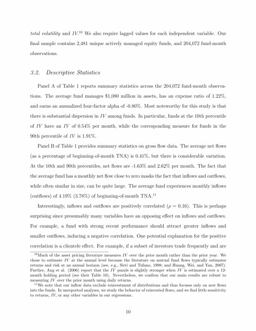
total volatility and IV.10 We also require lagged values for each independent variable. Our

final sample contains 2,481 unique actively managed equity funds, and 204,072 fund-month

observations.

3.2. Descriptive Statistics

Panel A of Table 1 reports summary statistics across the 204,072 fund-month observa-

tions. The average fund manages $1,080 million in assets, has an expense ratio of 1.22%,

and earns an annualized four-factor alpha of -0.80%. Most noteworthy for this study is that

there is substantial dispersion in IV among funds. In particular, funds at the 10th percentile

of IV have an IV of 0.54% per month, while the corresponding measure for funds in the

90th percentile of IV is 1.91%.

Panel B of Table 1 provides summary statistics on gross flow data. The average net flows

(as a percentage of beginning-of-month TNA) is 0.41%, but there is considerable variation.

At the 10th and 90th percentiles, net flows are -1.63% and 2.62% per month. The fact that

the average fund has a monthly net flow close to zero masks the fact that inflows and outflows,

while often similar in size, can be quite large. The average fund experiences monthly inflows

(outflows) of 4.19% (3.78%) of beginning-of-month TNA.11

Interestingly, inflows and outflows are positively correlated (ρ = 0.16). This is perhaps

surprising since presumably many variables have an opposing effect on inflows and outflows.

For example, a fund with strong recent performance should attract greater inflows and

smaller outflows, inducing a negative correlation. One potential explanation for the positive

correlation is a clientele effect. For example, if a subset of investors trade frequently and are

10Much of the asset pricing literature measures IV over the prior month rather than the prior year. Wechose to estimate IV at the annual level because the literature on mutual fund flows typically estimatesreturns and risk at an annual horizon (see, e.g., Sirri and Tufano, 1998; and Huang, Wei, and Yan, 2007).Further, Ang et al. (2006) report that the IV puzzle is slightly stronger when IV is estimated over a 12-month holding period (see their Table 10). Nevertheless, we confirm that our main results are robust tomeasuring IV over the prior month using daily returns.

11We note that our inflow data exclude reinvestment of distributions and thus focuses only on new flowsinto the funds. In unreported analyses, we study the behavior of reinvested flows, and we find little sensitivityto returns, IV, or any other variables in our regressions.

10

attracted to funds with certain characteristics, funds with these characteristics will likely

experience both greater inflows and outflows. Thus, examining net flows may conceal many

interesting patterns in the data.

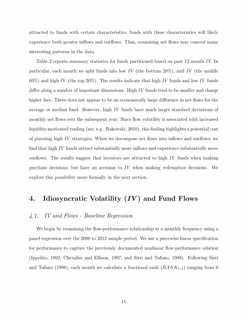
Table 2 reports summary statistics for funds partitioned based on past 12 month IV. In

particular, each month we split funds into low IV (the bottom 20%), mid IV (the middle

60%) and high IV (the top 20%). The results indicate that high IV funds and low IV funds

differ along a number of important dimensions. High IV funds tend to be smaller and charge

higher fees. There does not appear to be an economically large difference in net flows for the

average or median fund. However, high IV funds have much larger standard deviations of

monthly net flows over the subsequent year. Since flow volatility is associated with increased

liquidity-motivated trading (see, e.g., Rakowski, 2010), this finding highlights a potential cost

of pursuing high IV strategies. When we decompose net flows into inflows and outflows, we

find that high IV funds attract substantially more inflows and experience substantially more

outflows. The results suggest that investors are attracted to high IV funds when making

purchase decisions, but have an aversion to IV when making redemption decisions. We

explore this possibility more formally in the next section.

4. Idiosyncratic Volatility (IV ) and Fund Flows

4.1. IV and Flows - Baseline Regression

We begin by examining the flow-performance relationship at a monthly frequency using a

panel regression over the 2000 to 2012 sample period. We use a piecewise linear specification

for performance to capture the previously documented nonlinear flow-performance relation

(Ippolito, 1992; Chevalier and Ellison, 1997; and Sirri and Tufano, 1998). Following Sirri

and Tufano (1998), each month we calculate a fractional rank (RANKt−1) ranging from 0

11

to 1 for each fund based on the fund’s return over the prior 12 months.12 The variable Ret

Low is defined as Min(0.2, RANKt−1), while Ret Mid is defined as Min(0.6, RANKt−1 -

Ret Low). Finally, Ret High is defined as (RANKi,t−1 - .8) for funds in the top quintile of

performance and zero for all other funds. Our model takes on the following general form:

Flowi,t = α + β1RetLowi,t−1 + β2RetMidi,t−1 + β3RetHighi,t−1

+ β4SV i,t−1 + β5IV i,t−1 + γXi,t−1 + FE + εi,t (1)

In equation (1), the dependent variable, Flowi,t, is either the inflow, outflow, or net flow

expressed as a percentage of beginning-of-month TNA for each fund i and month t. Our

variable of primary interest is IV i,t−1, which measures the standard deviation of the fund’s

residuals from the Carhart (1997) four-factor model over the previous 12 months. We also

include SV i,t−1 which is the standard deviation of the fund’s returns over the previous 12

month less IV i,t−1.

Xi,t−1 is a vector of controls that consist of variables widely used in previous research. In

particular, we include Log age, Log size (fund TNA from the previous month), Log family size

(family TNA from the previous month), turnover ratio, expense ratio, and dummy variables

that indicate whether the fund charges loads (load fund), is closed to new investors during the

month (closed), or introduces a new share class in the period (new share class). In addition,

following Huang, Wei, and Yan (2007), we include the aggregate flow as a percentage of

aggregate assets for each Morningstar investment category in month t, to help control for

other unobserved factors, such as sentiment shifts towards certain styles that may influence

flows. All specifications include time fixed effects, and in Models 4-6 we also include fund

fixed effects. To ease interpretation of the results, we convert all continuous independent

variables (but not the dependent variable or the performance rank variables) to z -scores (the

12In unreported results, we estimate past performance using alternative horizons (e.g., returns over theprior 24 or 36 months) and alternative risk-adjustments (e.g., CAPM alphas or Carhart (1997) four-factoralphas) and find similar results.

12

values are de-meaned and then divided by their standard deviations). We cluster standard

errors by fund.13

Table 3 presents the results. Specifications 1, 2, and 3 report the results for net flows,

inflows, and outflows, respectively, prior to including fund fixed effects. Consistent with

existing studies, in Specification 1 we find that there is a strong relationship between net

flows and past performance.14 More relevant for our study, we find that a one standard

deviation increase in IV is associated with a modest 0.08 percentage point increase in net

flows.

Specifications 2 and 3, however, reveal that the patterns in net flows conceal a strong

relationship between IV and gross flows. Specifically, a one standard deviation increase in

IV is associated with a 0.84 percentage point increase in inflows (roughly a 20% increase

for the average fund) and a 0.84 percentage increase in outflows.15 Our results suggest that

current shareholders flee from IV when making redemption decisions (a seemingly rational

response), but new shareholders are attracted to funds with high IV (a seemingly irrational

response) when making purchase decisions.

Specifications 4 through 6 repeat the results after including fund fixed effects. We note

that IV is highly persistent at the fund-level, indicating that most of the variation in IV

occurs across funds rather than within funds. Despite the potentially lower power of this

test, we continue to find that investors are significantly more likely to both buy and sell a

given fund when it experiences an increase in IV.

In Table 4, we examine the robustness of the relation between IV and fund inflows and

outflows. In the interest of brevity, in each row we only report the coefficient on IV. For

reference, the first row of Table 4 reports the coefficient and t-statistic on IV from the

baseline results reported in Specifications 1 through 3 of Table 3.

13Clustering standard errors by both fund and time yields very similar results.14Unlike many prior studies, we find only modest evidence of a convex flow-performance relationship. This

finding is consistent with Kim (2013) who finds that the convex flow-performance relationship weakens after2000.

15We note that the coefficient on net flows does not equal the coefficient on inflows minus the coefficienton outflows because the controls for style-level flows differ across the three specifications.

13

One concern is that the relationship between IV and inflows is simply a manifestation

of investors buying last year’s extreme winners, which naturally tend to have higher IV.

Similarly, the positive relation between IV and outflows may reflect investors fleeing from

funds with extremely poor performance. To explore this possibility, we re-estimate the

baseline results separately for funds in the bottom, middle, and top tercile of past one-year

returns. The results, reported in Rows 2 through 4 of Table 4, are inconsistent with extreme

return chasing driving our main findings. For example, Row 3 documents a strong positive

relation between IV and inflows and outflows even for funds with average performance (i.e.,

funds in the middle tercile of performance).

Since net flows tend to be persistent (see, e.g., Coval and Stafford, 2007), it is also possible

that the ability of IV to predict flows is a consequence of IV proxying for past buying or

selling pressure. For example, a fund with extreme inflows may have very high returns (and

thus high IV ) due to price pressure as the fund purchases many of its existing positions.

An analogous but opposite pattern could arise for funds with extreme outflows. To explore

this possibility, we develop a measure of buying and selling pressure. Specifically, for each

fund i and month t, we compute Buying Pressure as: Max (0, NetF lowi,t). Similarly, we

define Selling Pressure as: Max (0, NetF lowi,t ×−1). Since IV is measured over the prior

12 months, we also sum Buying Pressure and Selling Pressure over the prior 12 months. In

Specification 5 of Table 4 we repeat our baseline specification after including Buying Pressure

and Selling Pressure. We find that the ability of IV to predict both inflows and outflows

is reduced, however the estimates remain highly significant.16 Thus, the ability of IV to

predict flows cannot be fully explained by past buying or selling pressure.

Rows 6 through 9 consider several additional robustness checks. First, in Row 6, following

Ang et al. (2006, 2009) we redefine IV as the standard deviation of the fund’s residuals from

the Fama-French (1993) three-factor model using daily returns over the previous calendar

16The reduced coefficient is a consequence of the significant contemporaneous correlation between IV andBuying Pressure (ρ = 0.12) and Selling Pressure (ρ = 0.11). Controlling for Buying Pressure and SellingPressure is appropriate if the contemporaneous correlation is driven by high inflows and outflows causingIV, but conservative if the correlation is driven by higher IV causing greater inflows and outflows.

14

month and find very similar results. Second, since many investors may not distinguish

between IV and SV (systematic volatility), in Row 7 we replace IV and SV with total

volatility.17 We continue to find that inflows and outflows are both significantly related to

total volatility. In Row 8, we repeat our analysis after excluding the month of December

and January and continue to find very similar results. This suggests that tax-loss selling

and other end-of-year adjustments are unlikely to drive our results. Finally, in Row 9, we

document very similar coefficients if we estimate Fama-Macbeth regressions, with Newey-

West standard errors, rather than panel regressions.

4.2. Are IV-Induced Capital Flows Informed?

Our results suggests that investors like IV when making purchase decisions, but dislike

IV when making redemption decisions. Purchases of high IV funds may be a consequence

of investors naturally gravitating towards funds with superior expected performance. Con-

sistent with this view, several recent measures of fund skill including industry concentration

(Kacperczyk, Sialm, Zheng, 2005), Active Share (Cremers and Petajisto, 2009), and R2

(Titman and Tiu, 2011; Amihud and Goyenko, 2013) are all correlated with IV. At the

same time, redemptions of high IV funds may reflect investors fleeing from a subset of high

IV funds with lower expected performance. In other words, if investors have the ability

to identify differential skill among mutual funds, and if this ability is amplified for funds

with higher IV, then we would expect high IV funds to experience both greater inflows and

greater outflows.

To explore this conjecture, in Table 5 we estimate the following panel regression:

Performancei,t = αi,t + β1IV i,t−1 + β2NetF lowi,t−1 + β3IV i,t−1 ×NetF lowi,t−1+

β4SV i,t−1 + γXi,t−1 + FE + εi,t (2)

17While much of the asset pricing literature has focused on the IV puzzle, other work highlights thepuzzling negative relationship between total volatility and returns including Haugen and Heins (1975) andBlitz and Van Vilet (2007).

15

where Performancei,t is either the return of fund i in month t in excess of the risk-free rate or

the alpha of fund i estimated from the Carhart (1997) four-factor model estimated using all

daily data in month t. Our main variables of interest include IVi,t−1, which explores whether

IV predicts superior fund performance; NetF lowi,t−1, which explores whether investors have

the ability to identify superior performing funds (i.e., the smart money effect); and IVi,t−1×

NetF lowi,t−1, which examines whether the smart-money effect is particularly pronounced

among funds with high IV. Xi,t−1 is a vector of controls that may also predict performance

including past performance, Log age, Log size, Log family size, turnover ratio, and expense

ratio. All independent variables are converted to z -scores. All regressions also include time

and style fixed effects, and standard errors are clustered by time.

Specifications 1 and 2 report results where the performance metric is the excess return.

Specification 1 (2) excludes (includes) IV i,t−1 ×NetF lowi,t−1. In Specification 1, we find a

positive, but economically small and statistically insignificant coefficient on IV, suggesting

that IV is not a strong predictor of fund performance. Similarly, we find a positive but

insignificant coefficient on Net Flow suggesting that investors are not able to identify superior

performing funds. In addition, in Specification 2, we find that the coefficient on IV ×

NetF low, is insignificant (and negative), which suggests that capital flows towards funds

with high IV cannot be explained by investors correctly identifying the best and worst

performing high IV funds. The results using fund alpha, reported in Specifications 3 and 4,

yield similar conclusions. Collectively, the evidence indicates that on average, capital flows

into and out of high IV funds do not forecast future returns.

4.3. Is IV A Risk Factor That Matters To Investors?

Another explanation that is consistent with the asymmetric relationship between IV and

inflows and outflows is risk. In particular, if investors view funds with low IV as riskier than

funds with high IV, then increases in IV may generate inflows (outflows) from more (less)

risk-averse investors. To test this possibility, we follow Berk and van Binsbergen (2016) and

16

Barber, Huang, and Odean (2016), and infer the risk model investors use by the fund choices

they make. Specifically, we assume that investor flows chase perceived past alpha, but do

not chase returns that stem purely from taking on extra risk. Thus, if investors chase returns

that are driven by exposure to a particular factor, investors are revealing that they view this

return as alpha rather than risk.

We begin by constructing an IV factor, LIVH (low IV minus high IV ). The construction

of the LIVH factor is similar to the approach outlined in Jordan and Riley (2015), except

we sort stocks on IV rather than total volatility. Specifically, when constructing the LIVH

factor, we only use the types of US equities commonly held by mutual funds: ordinary shares

(CRSP share codes 10 and 11) that trade on the NYSE, NASDAQ, or AMEX. After imposing

these filters, we sort stocks into deciles based on the standard deviation of a fund’s residuals

from a Carhart (1997) four-factor model using daily returns over the prior 12-months. The

LIVH factor is equal to the return on a value-weighted portfolio of stocks in the lowest decile

of IV less the return on a value-weighted portfolio of stocks in the highest decile of IV. We

find that the LIVH factor earns a significant three-factor alpha of 0.50% per month over our

sample period.

Using the framework of Barber, Huang, and Odean (2016), we decompose a fund’s returns

into a five-factor alpha and the returns that stem from factors related to market, size, value,

momentum, and IV tilts. Specifically, for each fund i in month t we estimate the following

time-series regression using return data from months τ = t-1 to t-60:18

Ri,τ −Rf,τ = αi,t + γi,tY DUM τ + β1i,t(Rm,τ −Rf,τ ) + β2i,tSMBτ

+ β3i,tHMLτ + β4i,tUMDτ + β5i,tLIVHτ + εi,τ (3)

where Ri,τ is the return of fund i in month τ , Rf,τ is the risk-free rate of return, Rm,τ

is the return on the value-weighted market index, SMBτ is the return on the size factor,

18If 60 months of historical data are not available we estimate the regression over all available data. Weexclude funds with less than 24 months of historical data.

17

HMLτ is the return on the value factor, UMDτ is the return on the momentum factor, and

LIV Hτ is the return on the IV factor. The returns on the market, size, book-to-market,

and momentum factors are obtained from Ken French’s online data library. The parameters

β1 − β5 represent the betas of the funds with respect to the market, size, value, momentum,

and IV factors; αi,t is the mean return unrelated to the factor exposures; and εi,τ is a mean

zero error term. Y DUM τ is a dummy variable equal to 1 for fund returns in the most recent

12-month period (τ = t-1 to t-12) and 0 otherwise. Thus, the estimated annual five-factor

alpha for the most recent 12-month period is αi,t + γi,t.

We next decompose a fund’s annual excess return into its alpha plus the return that is

attributed to tilts towards each of the five factors as follows:

Ri,t −Rf,t = (α̂i,t + γ̂i,t) + β̂1i,t(Rm,t −Rf,t) + β̂2i,t(SMBt)+

β̂3i,t(HMLt) + β̂4i,t(UMDt) + β̂5i,t(LIV H t) (4)

Ri,t −Rf,t is the average excess return of fund i over the prior 12 months (t-1 to t-12).

Similarly, (Rm,t −Rf,t) is the average market risk premium over the prior 12 months and β̂1i,t

is the fund’s estimated sensitivity to the market factor. Thus, β̂1i,t(Rm,t −Rf,t) captures the

return due to the fund’s exposure to the market factor. The remaining four terms capture the

returns due to the fund’s exposure to size, value, momentum, and IV factors, respectively.

To examine how investors respond to returns that stem from exposure to the IV factor,

we estimate the following panel regression:

Flowi,t = ψ0 +ψ1(α̂i,t + γ̂i,t) +ψ2

[β̂1i,t(Rm,t −Rf,t)

]+ψ3

[β̂2i,tSMBt)

]+ψ4

[β̂3i,tHMLt)

]+ ψ5

[β̂4i,tUMDt)

]+ ψ6

[β̂5i,tLIV H t)

]+ ψ7SV i,t−1 + ψ8IV i,t−1 + γXi,t−1 + FE + εi,t (5)

As in equation (1), Flowi,t, is either net flows, inflows, or outflows, expressed as a per-

centage of beginning-of-month TNA for each fund i and month t. SV i,t−1, IV i,t−1, and Xi,t−1

18

are defined as in equation (1). FE includes time fixed effects (in all specifications) and fund

fixed effects (in Specifications 4 through 6). The parameter of greater interest is ψ6, which

measures how investors respond to returns due to exposure to the IV factor.

Panel A of Table 6 reports the results. Not surprisingly, net flows are strongly related to

alpha; a one percentage point increase in alpha is associated with a 1.45 percentage point

increase in net flows. We also find that net flows are strongly related to returns traced to

the IV factor. Specifically, a one percentage point increase in returns due to IV exposure is

associated with a 0.86 percentage point increase in net flows. Alternatively, the estimated

coefficient on returns traced to IV risk is 59% (0.86/1.45) of the estimated coefficient on the

five-factor alpha. Similarly, using fund fixed effects (Specification 4) the estimated coefficient

on returns traced to IV risk is 65% (0.82/1.26) of the estimated coefficient on the five-factor

alpha. Thus, while investors discount returns that stem from IV risk, the magnitude of the

discount is relatively small.

It is also worth noting that controlling for a fund’s return due to its IV exposure has

very little impact on the conclusion that inflows and outflows are strongly associated with

the fund’s IV (i.e., ψ8). In other words, investors’ tendency to buy (or sell) funds with high

IV is not driven by simply chasing funds that earned extreme returns due to their exposure

to the IV factor.

One concern is that funds with high IV may have significant differences in risk exposures

that are not fully captured by the LIVH factor. For example, Fama and French (2016) show

that stocks with high IV are associated with companies that are less profitable and invest

more aggressively compared to low IV stocks. Accordingly, they find that the Fama and

French (2015) five-factor model, which adds factors formed on firm profitability (RMW ) and

investment (CMA) to the Fama and French (1993) three-factor model, explains a significant

portion of the IV puzzle in stocks. This finding points to the possibility that more risk-

averse mutual fund investors may gravitate towards high IV funds because such funds have

low exposure to the RMW and CMA risk factors.

19

To explore this possibility, we repeat equations (2) through (4), but now replace the UMD

and LIVH factors with the RMW and CMA factors from Ken French’s online data library.

The results of this analysis, presented in Panel B of Table 6, are consistent with the findings

from Panel A. In particular, Specification 1 indicates that the estimated coefficient on returns

traced to the RMW and CMA risk factors are 56% (0.77/1.38) and 76% (1.05/1.38) of the

estimated coefficient on the five-factor alpha. Similarly, Specification 4 confirms the results

are similar after including fund fixed effects. In addition, investors continue to be more

likely to both buy and sell funds with high IV even after the inclusion of the additional

risk factors. Collectively, the evidence suggests that flows into (out of) high IV funds are

unlikely to be entirely driven by investors who simply want to reduce (increase) the risk-level

of their portfolio.

5. Search Costs and the IV Puzzle

The evidence in Tables 3 through 6 appears at odds with many of the existing expla-

nations for the IV puzzle in stocks. For example, if the puzzle is simply driven by mi-

crostructure effects, it is unclear why investors exhibit a strong preference for IV when

purchasing mutual funds. Similarly, if the IV puzzle is driven purely by investors having

lottery-like preferences among mutual funds, it is unclear why investors shun high IV funds

when making redemption decisions. Further, the diversified nature of mutual funds makes

them relatively unattractive to investors with strong lottery-like preferences. Finally, the

findings that investors appear to chase returns traced to IV suggests that most investors

do not view returns due to exposure to the IV factor as compensation for risk. This is not

to say the above explanations do not contribute to fund investor behavior; however it does

suggest that other forces are likely at play.

Another line of reasoning that is consistent with the existing evidence is based on search

costs and limited attention. When faced with different options, individuals typically do

20

not pay equal attention to each option, but instead spend more time examining the most

salient (i.e., attention-grabbing) option. Funds with higher levels of IV are likely to be more

salient for at least some investors since high IV funds are more likely to appear in the media

(Kaniel, Starks, and Vasudevan, 2007) and are more likely to have extreme returns. Even

among funds with average returns over the prior year, high IV funds are more likely to have

extreme returns over other horizons (e.g., 1 day, 3 months, 5 years, etc.) that may be more

attention grabbing to particular investors.

To get a better sense for the relationship between IV and extreme returns, we sort mutual

funds into deciles based on past 12 month IV. For each decile, we examine the fraction of

funds that are in the top 10% of returns over the past three months or past five years

(extreme winners). We choose the three-month and five-year horizons, as this corresponds

to the shortest and longest window reported on Yahoo! Finance when screening for mutual

funds. The results reported in Figure 1 indicate that funds in the top decile of IV are

extreme winners 34% of the time at the five-year horizon (which reflects a 240% increase

relative to the unconditional probability of 10%) and 28% of the time at the three-month

horizon.

This finding suggests that high IV funds are more likely to catch the attention of investors

who tend to sort funds on past returns over very different horizons. While not all investors

will trade funds that catch their attention, it seems likely that funds that catch investors’

attention are more likely to be traded. Consistent with this view, Barber and Odean (2008)

find that investors tend to be net buyers of stocks with larger one-day returns. They argue

that attention-based trading is likely to be more prevalent for purchases, since investors tend

to only sell a small subset of all stocks - those they already own.

While limited attention and search costs may have a more pronounced impact on pur-

chase decisions, there is still good reason to believe that funds that catch investors’ attention

21

will also experience significantly larger capital outflows.19 First, even for investors holding

only a few funds, investors generally need an impetus to sell an existing position. Attention-

grabbing extreme returns can be the shock that causes investors to reconsider their current

positions. Further, conditional on needing to sell a fund, the “rank effect” documented by

Hartzmark (2015) suggests that investors are more likely to sell their extreme winning or

losing positions. Finally, if a subset of investors tend to purchase funds with high IV, such in-

vestors may also be more likely to sell funds with high IV. In other words, high IV funds may

attract a specific clientele of investors who tend to make purchase and redemption decisions

based on extreme returns or other attention-grabbing events (e.g., advertising). Thus, the

findings that high IV funds experience more purchases and redemptions is consistent with

limited attention and search costs influencing investor behavior (hereafter: the search-cost

hypothesis). We next examine whether the empirical evidence is consistent with additional

implications of the search-cost hypothesis.

5.1. IV and Fund Flows – Piecewise Regressions

The search-cost explanation for the asymmetric relationship between IV and flows points

to a possible non-linear relationship between IV and flows. For example, moving from the

1st percentile of IV to the 19th percentile of IV is unlikely to have significant effects on the

fund’s saliency, since the fund is still unlikely to have extreme returns. In contrast, moving

from the 80th percentile of IV to the 99th percentile of IV is likely to have a more dramatic

effect, since such funds will be increasingly more likely to be extreme winners or losers over a

variety of different return horizons. This view is consistent with the Figure 1 results, which

show that the relationship between IV and the likelihood of being an extreme winner is

highly convex.

19We also note that the positive (albeit economically modest) relationship between IV and net flows inTable 3 is consistent with Barber and Odean’s (2008) conjecture that the impact of limited attention shouldbe stronger for purchase decisions.

22

To explore the non-linear relationship between IV and flows, we replace IV i,t−1 with

an IV rank variable. Specifically, each month we calculate a fractional rank (RANKi,t−1)

ranging from 0 to 1 for each fund based on the fund’s IV. The variable IV Low is defined as

Min(0.2, RANKi,t−1), while IV Mid is defined as Min(0.6, RANKi,t−1 - IV Low). Finally,

IV High is zero for funds outside the top quintile of performers and equal to (RANKi,t−1 -

.8) for funds in the top quintile. We conduct an analogous adjustment for SV i,t−1. We then

estimate the following panel regression:

Flowi,t = α + β1RetLowi,t−1 + β2RetMidi,t−1 + β3RetHighi,t−1

+ β4SV Lowi,t−1 + β5SVMidi,t−1 + β6SV Highi,t−1

+ β7IV Lowi,t−1 + β8IVMidi,t−1 + β9IV Highi,t−1

+ γXi,t−1 + FE + εi,t (6)

where all other variables are defined as in equation (1). The coefficients of interest are β7 -

β9, which measures the sensitivity of flows to IV for different levels of IV.

Table 7 presents the results. Across all specifications, there is very little evidence that IV

is related to fund flows for funds in the bottom 20% of IV or for funds in the middle 60% of

IV. However, we document a strong relationship between inflows (or outflows) and IV for

funds in the top 20% of IV. In particular, Specifications 2 and 3 indicate that a 10 percentile

increase in a fund’s IV rank (e.g., moving from the 85th percentile to the 95th percentile)

is associated with a 1.02 percentage point increase in inflows and a 1.05 percentage point

increase in outflows. Our findings suggest that the relationship between inflows and outflows

and IV is driven by funds with the most extreme IV. Since such funds are the most likely

to have extreme returns, this pattern is consistent with the search-cost explanation. This

result is also consistent with the finding in the equity literature that the IV puzzle is largely

driven by the extremely poor performance of stocks in the top quintile of IV (Ang et al.,

2006).

23

5.2. IV and Fund Flows – Interactions with Search Costs

If search costs contribute to the strong relationship between IV and fund inflows and

outflows, then the relationship between IV and inflows and outflows should be weaker when

search costs are less severe. In this section, we empirically test this prediction using several

proxies for search costs.

First, we conjecture that search costs are likely to be less severe for larger funds, older

funds, funds that engage in greater marketing (Sirri and Tufano, 1998; Huang, Wei and

Yan, 2007), or funds with a five-star rating by Morningstar (Del Guercio and Tkac, 2008).

Intuitively, a larger fraction of potential investors are already aware of larger funds, older

funds, funds that frequently appear in the media, or funds that have a top rating by Morn-

ingstar, and thus extreme returns or other attention-grabbing events are likely to have a less

significant impact on the visibility of these funds relative to other funds. We also expect

that search costs are less severe for incumbent investors, who already own the fund and thus

are already aware of the fund’s existence.

Finally, we expect search costs to be less severe for institutional funds, which largely

reflect defined contribution (DC) plans. In DC plans, a menu of funds is initially selected

by plan sponsors. Plan sponsors, due to their greater sophistication and fiduciary responsi-

bilities, are less likely to have search costs influence their decision to add or remove funds.

Within the menu of investment options, IV is likely to be less relevant, since plan partici-

pants rarely adjust their pension allocations and generally have far fewer investment options

to evaluate.20

To examine whether the impact of IV on flows is stronger when search costs are more

severe, we estimate equation (1) after including the search cost variable and also interacting

the search cost variable with every other independent variable in the model. More specifically,

20Studies finding that plan participants often select the default investment options or rarely adjust theirallocations include: Madrian and Shea, 2001; Choi et al., 2002; and Sialm, Starks, and Zhang, 2015.

24

we examine the following panel regression:

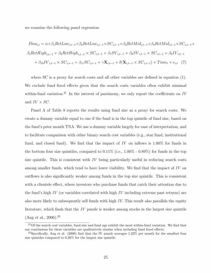
Flowi,t = α+β1RetLowi,t−1+β2RetLowi,t−1×SCi,t−1+β3RetMidi,t−1+β4RetMidi,t−1×SCi,t−1+

β5RetHighi,t−1 + β6RetHighi,t−1 × SCi,t−1 + β7SV i,t−1 + β8SV i,t−1 × SCi,t−1 + β9IV i,t−1

+ β10IV i,t−1 × SCi,t−1 + β11SCi,t−1 + γXi,t−1 + δ(Xi,t−1 × SCi,t−1) + Timet + εi,t (7)

where SC is a proxy for search costs and all other variables are defined in equation (1).

We exclude fund fixed effects given that the search costs variables often exhibit minimal

within-fund variation.21 In the interest of parsimony, we only report the coefficients on IV

and IV × SC.

Panel A of Table 8 reports the results using fund size as a proxy for search costs. We

create a dummy variable equal to one if the fund is in the top quintile of fund size, based on

the fund’s prior month TNA. We use a dummy variable largely for ease of interpretation, and

to facilitate comparison with other binary search cost variables (e.g., star fund, institutional

fund, and closed fund). We find that the impact of IV on inflows is 1.00% for funds in

the bottom four size quintiles, compared to 0.11% (i.e., 1.00% - 0.89%) for funds in the top

size quintile. This is consistent with IV being particularly useful in reducing search costs

among smaller funds, which tend to have lower visibility. We find that the impact of IV on

outflows is also significantly weaker among funds in the top size quintile. This is consistent

with a clientele effect, where investors who purchase funds that catch their attention due to

the fund’s high IV (or variables correlated with high IV including extreme past returns) are

also more likely to subsequently sell funds with high IV. This result also parallels the equity

literature, which finds that the IV puzzle is weaker among stocks in the largest size quintile

(Ang et al., 2006).22

21Of the search cost variables, fund size and fund age exhibit the most within-fund variation. We find thatour conclusions for these variables are qualitatively similar when including fund fixed effects.

22Specifically, Ang et al. (2006) find that the IV puzzle averages 1.23% per month for the smallest foursize quintiles compared to 0.26% for the largest size quintile.

25

In Panels B and C, the search cost proxy is a dummy variable equal to one if the fund

is in the top quintile of fund age and fund marketing expenditures, respectively. Following

Huang, Wei, and Yan (2007), we measure marketing expenses as the 12b-1 fees + 1/7th of

the front-end load. In Panel D, the search cost proxy is a dummy variable equal to one if

the fund is rated 5-stars by Morningstar. The results from Panels B, C, and D indicate that

the impact of IV on fund inflows (or outflows) is significantly weaker for older funds, funds

that engage in greater marketing, and star funds.

Panel E of Table 8 presents results where the search cost measure is a dummy variable

equal to one if the fund is closed to new investors. Note that flows in closed funds only

reflect the investment decisions of incumbent investors who are already aware of the fund.

We find that the relationship between IV and inflows is significantly weaker for closed funds.

Similarly, the relationship between IV and outflows is significantly weaker for closed funds.

This is perhaps surprising, since outflows for both open and closed funds reflect the invest-

ment decisions of incumbent investors. However, the composition of existing investors in

open versus closed funds is likely different. In particular, open funds with high IV attract

many investors who gravitate towards attention-grabbing funds. These same investors ap-

pear prone to quickly selling the fund. Thus, as the fund remains closed, the clientele shifts

towards investors who are less likely to be influenced by a fund’s past IV when making their

redemption decisions.

Finally, Panel F of Table 8 examines whether the results differ for retail versus insti-

tutional funds. Specifically, we include an institutional fund indicator which equals one if

all the share classes of the fund are classified as institutional by CRSP and zero if all the

share classes of the fund are classified as retail.23 Roughly 13% of the funds are classified

as institutional and 42% are classified as retail. The remaining funds either have a mix of

retail and institutional share classes or provide no indication of the intended investor. Only

23In untabulated analysis, we also define a fund as institutional based on its minimum investment size.Defining a fund as institutional if the minimum investment size is greater than or equal to $10,000 (or$100,000) generates very similar results.

26

funds with 100% institution or 100% retail are included in Panel F of Table 8. The results

confirm that the relationship between IV and flows is stronger among retail-oriented funds.

In particular, for retail funds, a one standard deviation increase in IV is associated with a

1.09 percentage point increase in inflows and a 1.14 percentage point increase in outflows.

The corresponding estimates for institutional funds are 0.09 and 0.26, neither of which is

significantly different from zero. Collectively, the results from Tables 8 support the notion

that the impact of IV on fund flows is stronger when search costs are more severe.

5.3. IV, Google Search, and Fund Flows

Our evidence is consistent with the views that 1) IV results in increased investor atten-

tion, 2) increased investor attention results in greater inflows and outflows, and 3) the impact

of increased investor attention on inflows and outflows is greater when search costs are more

severe. In this section, we offer more direct evidence for each of the above conjectures using

Google search volume as a proxy for investor attention (as in Da, Engelberg, and Gao, 2011).

5.3.1. Google Search Methodology

We collect the monthly normalized search volume index (NSVI ), as reported by Google

Trends, for each fund ticker from January 2004 (the begin date for Google Trends data)

through December 2012.24 To increase the likelihood that our search reflects demand for

information about mutual funds, we limit the search region to the “United States” and the

search category to “Business”.25

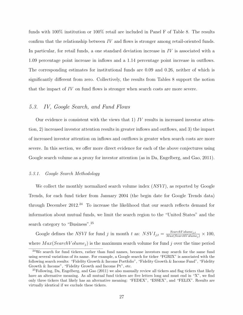
Google defines the NSVI for fund j in month t as: NSV Ij,t =SearchV olumej,t

Max(SearchV olumej)× 100,

where Max(SearchV olumej) is the maximum search volume for fund j over the time period

24We search for fund tickers, rather than fund names, because investors may search for the same fundusing several variations of its name. For example, a Google search for ticker “FGRIX” is associated with thefollowing search results: “Fidelity Growth & Income Portfolio”, “Fidelity Growth & Income Fund”, “FidelityGrowth & Income”, “Fidelity Growth and Income Pt”, etc.

25Following, Da, Engelberg, and Gao (2011) we also manually review all tickers and flag tickers that likelyhave an alternative meaning. As all mutual fund tickers are five letters long and must end in “X”, we findonly three tickers that likely has an alternative meaning: “FEDEX”, “ESSEX”, and “FELIX”. Results arevirtually identical if we exclude these tickers.

27

of the search. By scaling by Max(SearchV olumej), NSVI abstracts from cross-sectional

differences in search volume. For example, a large fund with a maximum monthly search

volume of 1,000 and a small fund with a maximum monthly search volume of 10 would both

report a maximum NSVI of 100. More generally, across all months the large funds’ NSVI

would be understated by a factor of 100 (1000/10) relative to the small funds’ NSVI.

To circumvent this limitation, we estimate a scaling factor that accurately portrays the

relative popularity of each fund.26 To create the scaling factor for fund j relative to fund

k (Scalingj,k) we first collect the monthly values of NSV Ij and NSV Ik from two inde-

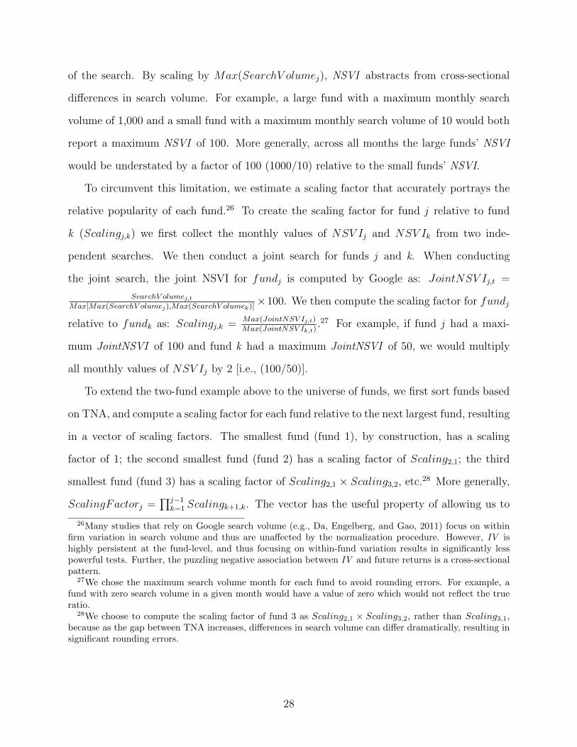
pendent searches. We then conduct a joint search for funds j and k. When conducting

the joint search, the joint NSVI for fundj is computed by Google as: JointNSV Ij,t =

SearchV olumej,tMax[Max(SearchV olumej),Max(SearchV olumek)]

×100. We then compute the scaling factor for fundj

relative to fundk as: Scalingj,k =Max(JointNSV Ij,t)

Max(JointNSV Ik,t).27 For example, if fund j had a maxi-

mum JointNSVI of 100 and fund k had a maximum JointNSVI of 50, we would multiply

all monthly values of NSV Ij by 2 [i.e., (100/50)].

To extend the two-fund example above to the universe of funds, we first sort funds based

on TNA, and compute a scaling factor for each fund relative to the next largest fund, resulting

in a vector of scaling factors. The smallest fund (fund 1), by construction, has a scaling

factor of 1; the second smallest fund (fund 2) has a scaling factor of Scaling2,1; the third

smallest fund (fund 3) has a scaling factor of Scaling2,1 × Scaling3,2, etc.28 More generally,

ScalingFactorj =∏j−1

k=1 Scalingk+1,k. The vector has the useful property of allowing us to

26Many studies that rely on Google search volume (e.g., Da, Engelberg, and Gao, 2011) focus on withinfirm variation in search volume and thus are unaffected by the normalization procedure. However, IV ishighly persistent at the fund-level, and thus focusing on within-fund variation results in significantly lesspowerful tests. Further, the puzzling negative association between IV and future returns is a cross-sectionalpattern.

27We chose the maximum search volume month for each fund to avoid rounding errors. For example, afund with zero search volume in a given month would have a value of zero which would not reflect the trueratio.

28We choose to compute the scaling factor of fund 3 as Scaling2,1 × Scaling3,2, rather than Scaling3,1,because as the gap between TNA increases, differences in search volume can differ dramatically, resulting insignificant rounding errors.

28

estimate the popularity of fundj relative to the smallest fund. To reduce the influence of

outliers, we winsorize the scaling factor at the 99th percentile.

Our primary measure of interest is Search defined as NSV Ij,t multiplied by the scaling

factor for fund j. We compute a fund-level measure of Search by summing the Search of

each ticker (i.e., share class) of the fund. Our final sample includes 164,378 fund-month

Search observations over the 2004-2012 period. We find that Search exhibits significant

cross-sectional variation; the mean (median) value of Search is 3,466 (0) and the standard

deviation is 13,209. To the extent that Search is a good measure of investor attention, our

findings suggest that while a few funds garner massive amounts of attention, the typical fund

attracts very little investor attention.

5.3.2. Google Search Results

We now turn to testing our three conjectures outlined in Section 5.3. We begin by

examining whether funds with greater IV also experience greater Search. We expect that

many of the same factors that drive purchase and redemption decisions will also drive search

volume. Accordingly, we re-estimate the baseline flow regression (i.e., equation (1)) after

replacing the dependent variable Flowi,t, with Log(1 + Searchi,t). In the interest of brevity,

we only report the coefficient on IV, past returns, and fund size.

The results are reported in Column 1 of Table 9. Intuitively, large funds have greater

Search. In addition, the positive coefficient on RetHigh and the negative coefficient on RetLow

indicate that Search tends to increase with either extremely good or extremely bad past one-

year performance. However, even after controlling for extreme past one-year returns, we find

a strong positive relation between IV and Search. In particular, a one-standard deviation

increase in IV is associated with a roughly 66% increase in Search. This finding suggests

that funds with greater IV garner greater investor attention.

We next examine whether Search forecasts greater inflows and outflows. We re-estimate

equation (1) after replacing IVi,t−1 with Log(1 + Searchi,t−1). Columns 2 through 4 report

29

the results for net flows, inflows, and outflows, respectively. We find that a one standard

deviation increase in average monthly Search over the prior 12 months is associated with a

0.41 percentage point increase in monthly inflows and a 0.21 percentage point increase in

outflows, both of which are highly significant. This finding supports the view that increased

investor attention leads to greater capital inflows and outflows.29 We also find that Search

is significantly positively associated with net flows, consistent with investor attention having

a larger effect on buying decisions than selling decisions.

We also re-estimate equation 1 after including both IVi,t−1 and Log(1+Searchi,t−1). This

test examines whether IV and Search contain independent information about future flows.

Examining inflows (Column 6), we find that both IV and Search are incrementally useful in

forecasting flows and the difference between the two estimates is not statistically significant.

This is consistent with both IV and Search containing distinct information about investor

attention.30 However, examining outflows (Column 7), we find that IV remains significantly

positive, while Search is no longer significantly different from zero. As noted earlier, the

positive coefficient on IV is consistent with extreme returns making it more likely that an

investor will reconsider his position in the fund. In addition, it increases the likelihood

that investors subject to the rank effect bias (Hartzmark, 2015) will sell the fund. The

insignificant coefficient on Search is consistent with the view that existing investors, who

are very familiar with the fund, generally do not need to conduct additional research before

selling the fund.

Finally, we examine whether the impact of increased investor attention on inflows and

outflows is greater when search costs are more severe. Our approach mirrors equation (7)

29In unreported results, we also estimate a model with fund fixed effects. We continue to find positivecoefficients, but the magnitudes decline, and the estimate for outflows loses statistical significance.

30For example, an investor who identifies a high IV fund by sorting on past three-month performance onYahooFinance, may simply learn more about the fund by searching within YahooFinance (i.e., high IV, butno Search). More generally, Search is an imperfect proxy for attention since it is limited to Google searchesfor the fund ticker. On the other hand, a prominent news story about a fund manager may not be causedby extreme returns, but can lead to significant search volume (i.e., high Search, but no IV ).

30

except we replace IVi,t−1 with Log(1+Searchi,t−1). Table 10 reports the results for the same

six measures of search costs analyzed in Table 8.

We generally find that increased investor attention has a larger effect on inflows and

outflows when search costs are more severe. For example, Panel A shows the impact of

Search on both inflows and outflows is significantly weaker for large funds (i.e., funds in

the top TNA quintile). More generally, in 11 out of 12 cases, we find that the impact of

Search on inflows and outflows is greater when search costs are more severe, and the effect is

statistically significant (at a 5% level) in 5 of the 12 cases. Collectively, the results from this

section provide more direct evidence that IV is associated with increased investor attention,

and confirm that increased investor attention is associated with greater capital inflows and

capital outflows, particularly among funds with greater search costs.

6. Conclusion

A growing literature finds that assets with high IV earn low returns, which points to

the puzzling possibility that investors prefer assets with high IV. We re-examine investors’

preferences toward IV by studying their capital flows into and out of mutual funds. We find

that both inflows and outflows are strongly related to IV, indicating that investors gravitate

towards IV when making purchasing decisions, but flee from IV when making redemption

decisions. We find no evidence that purchases or redemptions of funds with high IV are

associated with superior returns, which suggests that informed trading cannot explain our

findings. We also find that flows chase returns that stem from a fund’s exposure to IV risk

factors, suggesting that majority of capital does not view IV as a risk factor.

The above evidence suggests that many existing explanations for the IV puzzle, including

risk-based explanations (e.g., Chen and Petkova, 2012) or microstructure biases (e.g., Fu

2009) cannot fully explain investors’ preferences for IV among mutual funds. Instead, we

propose that limited attention and search costs can help explain fund investors’ asymmetric

31

preference for IV. Intuitively, assets with greater IV are more salient and therefore more likely

to catch the attention of investors. Thus, high IV assets are more likely to be purchased by

attention-based traders (Barber and Odean, 2008). Attention-based traders are also more

likely to sell assets with more extreme returns (Hartzmark, 2015), resulting in the asymmetric

pattern where investors gravitate towards IV when making purchasing decisions, but flee

from IV when making redemption decisions.

We offer several novel pieces of evidence consistent with limited attention and search costs

driving investors’ asymmetric preferences for IV. First the impact of IV on flows is greater

among funds where search costs are more severe including smaller funds, younger funds, funds

that engage is less marketing, non-star funds, funds that are not closed to new investors,

and retail funds. Second, we find that funds with higher IV garner more investor attention,

as measured by Google search volume. Finally, funds with greater investor attention (i.e.,

funds with larger Google search volume) experience greater inflows and outflows, particularly

when search costs are more severe.

Although investors’ preferences for mutual funds may be driven by different considera-

tions than their preferences for individual equities, our findings are consistent with many

of the findings from the equity literature. For example, we find that the impact of IV on

flows is concentrated in the top quintile of IV. This result is compatible with the equity

literature, which finds that the IV puzzle is driven by the extremely low returns of equities

in the top quintile of IV (Ang et al., 2006). Similarly, the finding that mutual fund investors’

preference for IV is concentrated among retail investors, who presumably face greater search

costs, is consistent with the finding that the IV puzzle tends to be stronger among stocks

with a less sophisticated investor base (Jiang, Xu, and Yao, 2009).

Given these similarities, the search cost explanation explored in this study may also help

explain the IV puzzle among equities. In particular, if IV increases the saliency of mutual

funds, it is plausible that IV also increases the saliency of equities, which can result in

improved investor recognition and liquidity, and ultimately a lower required rate of return

32

(see, e.g., Amihud and Mendelson, 1986; and Kadlec and McConnell, 1994). In short, while

we cannot draw broader conclusions about the role of IV and saliency for individual stocks

from this study, the consistencies we observe suggest that exploring this possibility may be

a promising area for future research.

33

Appendix: Variable Definitions

Note: Unless otherwise stated, we aggregate multiple share classes of a fund into one obser-

vation by computing a TNA-weighted average across all share classes.

• Inflow: the monthly new inflow of a fund scaled by the fund’s TNA at the begin-

ning of the month (Source: Morningstar). This measure excludes the reinvestment of

distributions.

• Outflow: the monthly new outflow of a fund scaled by the fund’s TNA at the beginning

of the month (Source: Morningstar).

• Net Flow: Inflow - Outflow.

• Standard Deviation Net Flow: The time-series standard deviation in monthly Net Flow

for a fund over a specified time period.

• Style Flow: the average monthly flow (i.e., Inflow, Outflow, or Net Flow) across all

funds in a given style. Style classifications are based on Morningstar investment cate-

gories (Source Morningstar).

• Total Volatility (TV): the standard deviation of a fund’s returns of the prior 12 months

(Source: CRSP/Morningstar).

• Idiosyncratic Volatility (IV): the standard deviation of the fund’s residual from the

Carhart (1997) four-factor model over the previous 12 months (Source: CRSP/Morningstar).

• Systematic Volatility (SV): Total Volatility - Idiosyncratic Volatility.

• Return: the average monthly returns over the prior 12 months (Source: CRSP/Morningstar).

• RANK: the percentile ranking of a fund based on its Return.

• Ret Low: Min (.2, RANK).

• Ret Mid: Min(.6, RANK - Ret Low).

• Ret High: Max (RANK - .8, 0).

• Carhart Alpha: the alpha from a regression of the fund’s return on the Carhart (1997)

four-factor model, estimated using monthly returns over the prior 12 months (Source:

CRSP/Morningstar).

34

• Total Net Assets (TNA): the total amount of money managed by the fund ($ millions)

(Source: CRSP/Morningstar).

• Family TNA: the total amount of money managed by the family across all funds that

appear in CRSP ($ millions) (Source: CRSP/Morningstar).

• Age: The number of months since the first offer date for the oldest share class of the

fund (Source: Morningstar).

• Expense Ratio: the annual expense ratio (Source: CRSP).

• Turnover Ratio: the annual turnover ratio (Source: CRSP).

• New Share Class: a dummy variable equal to one if the fund introduced a new share

class within the past year (Source: CRSP).

• Load Fund: a dummy variable equal to one if the fund charges either a front-end or

back-end load. (Source: CRSP).

• Marketing Expenditures: the sum of a fund’s 12b-1 fees and 1/7 of front-end loads

(Source: CRSP).

• Star Fund: a dummy variable equal to one if the fund is assigned a five-star rating

based on the past three-year performance (Source: Morningstar).

• Closed: a dummy variable equal to one if the fund is closed to new investors (Source:

CRSP).

• Institutional Fund: a dummy variable equal to one if the fund serves institutional

investors, and zero otherwise (Source: CRSP).

• Search: a ticker’s normalized search volume (NSVI) from Google Trends multiplied by

a scaling factor that estimates the relative popularity of a fund relative to the smallest

fund. Section 5.3.1 provides additional details on the NSVI data and the construction

of the scaling factor. (Source: Google Trends).

35

References

Amihud, Yakov, Ruslan Goyenko. 2013. Mutual fund’s r2 as predictor of performance.Review of Financial Studies , 26 667–694.

Amihud, Yakov, Haim Mendelson. 1986. Asset pricing and the bid-ask spread. Journal ofFinancial Economics , 17 223–249.

Ang, Andrew, Robert J. Hodrick, Yuhang Xing, Xiaoyan Zhang. 2006. The cross-section ofvolatility and expected returns. Journal of Finance, 61 259–299.

Ang, Andrew, Robert J. Hodrick, Yuhang Xing, Xiaoyan Zhang. 2009. High idiosyncraticvolaitility and low returns: Interantional and further US evidence. Journal of FinancialEconomics , 91 1–23.

Bali, Turan G., Nurset Cakici, Robert F. Whitelaw. 2011. Maxing out: Stocks as lotteriesand the cross-section of expected returns. Journal of Financial Economics , 99 427–446.

Bali, Turan G., Nusret Cakici. 2008. Idiosyncratic volatility and the cross section of expectedreturns. Journal of Financial and Quantitative Analysis , 43 29–58.

Barber, Brad, Xing Huang, Terrance Odean. 2016. Which risk factors matter to investors?evidence from mutual fund flows. The Review of Financial Studies, Forthcoming .

Barber, Brad, Terrance Odean. 2008. All that glitters: The effect of attention and newson the buying behavior of individual and institutional investors. The Review of FinancialStudies , 21 785–818.

Barber, Brad, Terrance Odean, Lu Zheng. 2005. Out of sight, out of mind: The effects ofexpenses on mutual fund flows. Journal of Business , 78 2095–2119.

Barberis, Nicholas, Ming Huang. 2008. Stocks as lotteries: The implications of probabilityweighting for security prices. American Economic Review , 98 2066–2100.

Barberis, Nicholas, Wei Xiong. 2012. Realization utility. Journal of Financial Economics ,104 251–271.

Berk, Jonathan, Jules van Binsbergen. 2015. Measuring skill in the mutual fund industry.Journal of Financial Economics , 118 1–20.

Berk, Jonathan, Jules van Binsbergen. 2016. Assessing asset pricing models using revealedpreferences. Journal of Financial Economics , 119 1–23.

Blitz, David, Plim van Vilet. 2007. The volatility effect: Lower risk without lower return.Journal of Portfolio Management , 34 102–113.

Bodnaruk, Andriy, Per Ostberg. 2009. Does investor recognition predict returns? Journalof Financial Economics , 91 208–226.

36

Boyer, Brian, Todd Mitton, Keith Vorkink. 2010. Expected idiosyncratic skewness. Reviewof Financial Studies , 23 169–202.

Carhart, Mark. 1997. On persistence in mutual fund performance. Journal of Finance, 5257–82.

Chen, Honghui, Gregory Noronha, Vijay Singal. 2004. The price response to S&P 500index additions and deletions: Evidence of asymmetry and a new explanation. Journal ofFinance, 59 1901–1929.

Chen, Zhanhui, Ralitsa Petkova. 2012. Does idiosyncratic volatility proxy for risk exposure?Review of Financial Studies , 25 2745–2787.

Chevalier, Judith, Glenn Ellison. 1997. Risk taking by mutual funds as a response to incen-tives. Journal of Political Economy , 105 1167–1200.

Choi, James, David Laibson, Brigitte Madrian, Andrew Mettrick. 2002. Defined contributionpensions: Plan rules, participant decisions, and the path of least resistance. Cambridge,MA: MIT Press.

Chordia, Tarun. 1996. The structure of mutual fund charges. Journal of Financial Eco-nomics , 41 3–39.

Coval, Joshua, Eric Stafford. 2007. Asset fire sales (and purchases) in equity markets. Journalof Financial Economics , 86 479–512.

Cremers, Martijn, Antti Petajisto. 2009. How active is your fund manager? a new measurethat predicts performance. Review of Financial Studies , 22 3329–3365.

Da, Zhi, Joseph Engelberg, Pengjie Gao. 2011. In search of attention. The Journal ofFinance, 66 1461–1499.

Del Guercio, Diane, Paula Tkac. 2008. Star power: The effect of morningstar ratings onmutual fund flow. Journal of Financial and Quantitative Analysis , 43 907–936.

Edelen, Roger. 1999. Investor flows and the assessed performance of open-end mutual funds.Journal of Financial Economics , 53 439–436.

Fama, Eugene, Kenneth French. 1993. Common risk factors in the returns on stocks andbonds. Journal of Financial Economics , 33 3–56.

Fama, Eugene, Kenneth French. 2015. A five-factor asset pricing model. Journal of FinancialEconomics , 116 1–22.

Fama, Eugene, Kenneth French. 2016. Dissecting anomalies with a five-factor model. Reviewof Financial Studies Forthcoming.

Fu, Fangjian. 2009. Idiosyncratic risk and the cross-section of expected stock returns. Journalof Financial Economics , 91 24–37.

37

George, Thomas, Chuan-Yang Hwang. 2011. Analyst coverage and the cross sectional relationbetween returns and volatility. Working Paper, University of Houston.

Green, T. Clifton, Russell Jame. 2013. Company name fluency, investor recognition, andfirm value. Journal of Financial Economics , 109 813–834.

Han, Yufeng, David Lesmond. 2011. Liquidity biases and the pricing of cross-sectionalidiosyncratic volatility. Review of Financial Studies , 24 1590–1629.

Hartzmark, Samuel. 2015. The worst, the best, ignoring all the rest: The rank effect oftrading behavior. Review of Financial Studies , 28 1024–1059.

Haugen, Robert, James Heins. 1975. Risk and the rate of return on financial assets: Someold wine in new bottles. Journal of Financial and Quantitative Analysis , 10 775–784.

Huang, Jennifer, Kelsey Wei, Hong Yan. 2007. Participation costs and the sensitivity of fundflows to past performance. Journal of Finance, 62 1273–1311.

Huang, Wei, Quianqiu Liu, Ghon Rhee, Liang Zhang. 2009. Return reversals, idiosyncraticrisk, and expected returns. Review of Financial Studies , 23 146–168.

Ippolito, Richard. 1992. Consumer reaction to measures of poor quality: evidence from themutual fund industry. Journal of Law and Economics , 35 45–70.

Jiang, George, Danielle Xu, Tong Yao. 2009. The information content of idiosyncratic volatil-ity. Journal of Financial and Quantitative Analysis , 44 147–168.

Johnson, Timothy. 2004. Forecast dispersion and the cross-section of stock returns. Journalof Finance, 59 1957–1978.

Jordan, Bradford, Timothy Riley. 2015. Volatility and mutual fund manager skill. Journalof Financial Economics , 118 289–298.

Kacperczyk, Marcin, Clemens Sialm, Lu Zheng. 2005. On the industry concentration ofactively managed equity mutual funds. The Journal of Finance, 60 19832011.

Kadlec, Gregory, John McConnell. 1994. The effect of market segmentation and liquidity onasset prices: Evidence from exchange listings. Journal of Finance, 49 611–636.

Kaniel, Ron, Robert Parham. 2015. WSJ category kings - The impact of media attentionon consumer and mutual fund investment decisions. Journal of Financial EconomicsForthcoming.

Kaniel, Ron, Laura Starks, Vasudha Vasudevan. 2007. Headlines and bottom lines: Attentionand learning effects from media coverage of mutual funds. Working Paper, University ofRochester .

Kim, Min. 2013. Changes in mutual fund flows and managerial incentives. Working Paper,University of New South Wales .

38

Lintner, John. 1965. The value of risk assets and the selection of risky investments in stockportfolios and capital budgets. Review of Economics and Statistics , 47 13–37.

Madrian, Brigitte, Dennis Shea. 2001. The power of suggestion: Inertia in 401(k) participa-tion and savings behavior. Quarterly Journal of Economics , 116 1149–1187.

Merton, Robert C. 1987. A simple model of capital market equilibrium with incompleteinformation. Journal of Finance, 42 483–510.

Pastor, Lubos, Robert Stambaugh, Lucian Taylor. 2015. Scale and skill in active manage-ment. Journal of Financial Economics , 116 23–45.

Rachwalski, Mark, Quan Wen. 2016. Idiosyncratic risk innovations and the idiosyncraticrisk-return relation. Review of Asset Pricing Studies Forthcoming.

Rakowski, David. 2010. Fund flow volatility and performance. Journal of Financial andQuantitative Analysis , 45 223–237.

Sensoy, Berk. 2009. Performance evaluation and self-designated benchmark indexes in themutual fund industry. Journal of Financial Economics , 92 25–39.

Sharpe, William. 1964. Capital asset prices: A theory of market equilibrium under conditionsof risk. Journal of Finance, 19 425–442.

Sialm, Clemens, Laura Starks, Hanjiang Zhang. 2015. Defined contribution pension plans:Stick or discerning money? Journal of Finance, 70 805–838.

Sirri, Erik, Peter Tufano. 1998. Costly search and mutual fund flows. Journal of Finance,53 1589–1622.

Stambaugh, Robert, Jiangfeng Yu, Yu Yuan. 2015. Arbitrage asymmetry and the idiosyn-cratic volatility puzzle. Journal of Finance Forthcoming.

Titman, Sheridan, Cristian Tiu. 2011. Do the best hedge funds hedge? Review of FinancialStudies 123–168.

Yuan, Yu. 2015. Market-wide attention, trading, and stock returns. Journal of FinancialEconomics , 116 548–564.

39

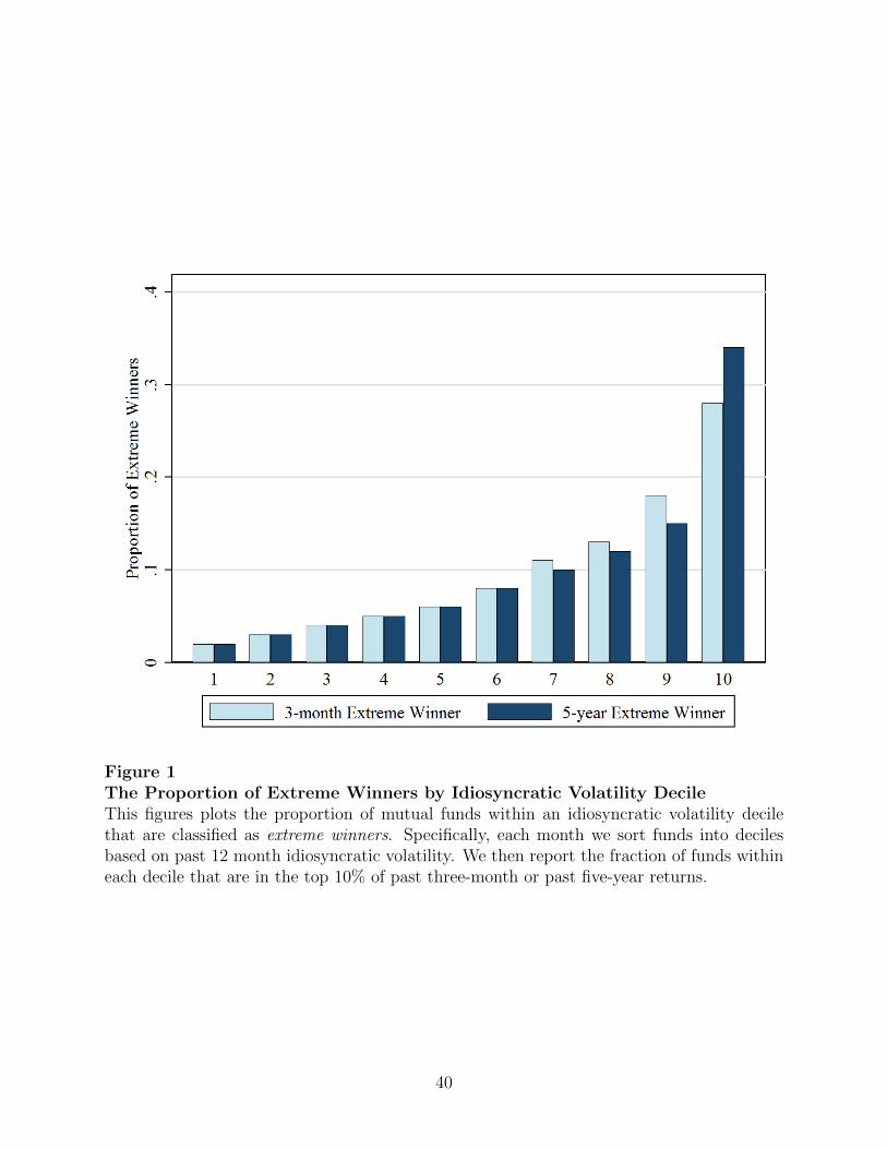
Figure 1The Proportion of Extreme Winners by Idiosyncratic Volatility DecileThis figures plots the proportion of mutual funds within an idiosyncratic volatility decilethat are classified as extreme winners. Specifically, each month we sort funds into decilesbased on past 12 month idiosyncratic volatility. We then report the fraction of funds withineach decile that are in the top 10% of past three-month or past five-year returns.

40

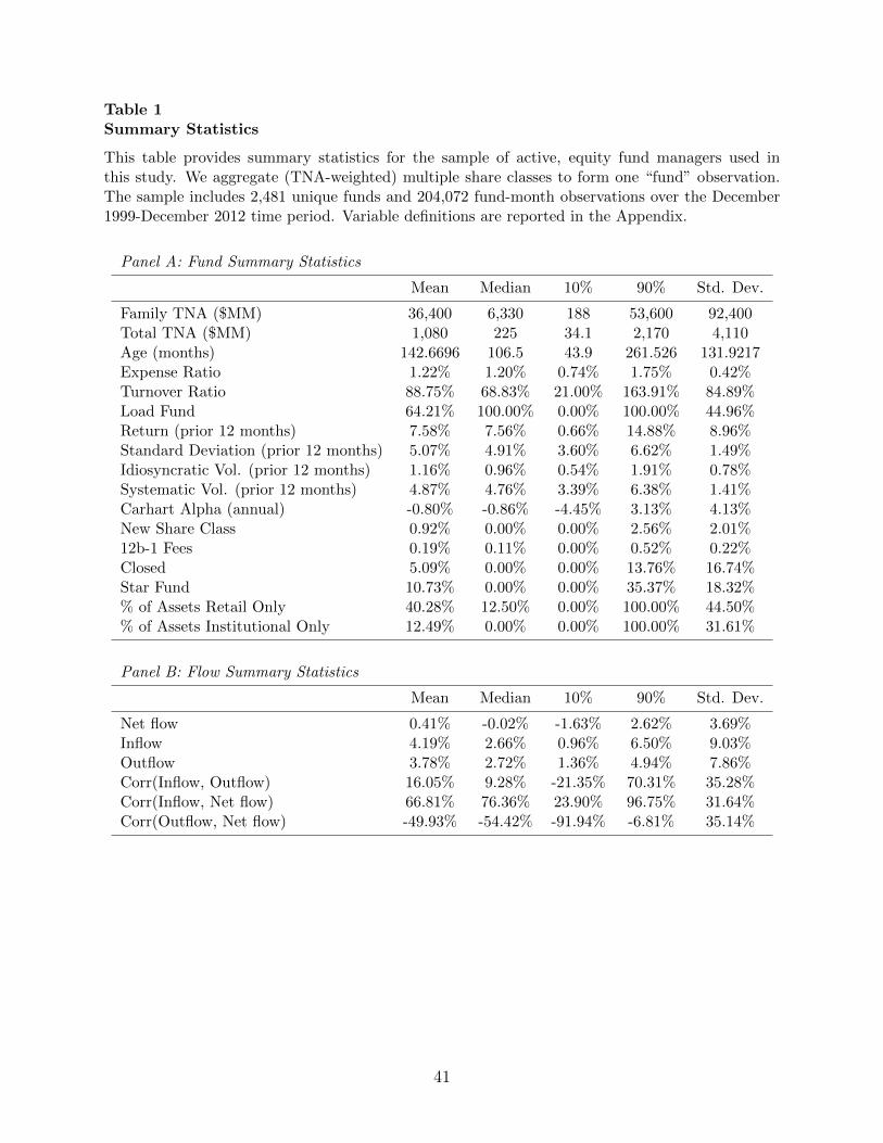
Table 1Summary Statistics

This table provides summary statistics for the sample of active, equity fund managers used inthis study. We aggregate (TNA-weighted) multiple share classes to form one “fund” observation.The sample includes 2,481 unique funds and 204,072 fund-month observations over the December1999-December 2012 time period. Variable definitions are reported in the Appendix.

Panel A: Fund Summary Statistics

Mean Median 10% 90% Std. Dev.

Family TNA ($MM) 36,400 6,330 188 53,600 92,400Total TNA ($MM) 1,080 225 34.1 2,170 4,110Age (months) 142.6696 106.5 43.9 261.526 131.9217Expense Ratio 1.22% 1.20% 0.74% 1.75% 0.42%Turnover Ratio 88.75% 68.83% 21.00% 163.91% 84.89%Load Fund 64.21% 100.00% 0.00% 100.00% 44.96%Return (prior 12 months) 7.58% 7.56% 0.66% 14.88% 8.96%Standard Deviation (prior 12 months) 5.07% 4.91% 3.60% 6.62% 1.49%Idiosyncratic Vol. (prior 12 months) 1.16% 0.96% 0.54% 1.91% 0.78%Systematic Vol. (prior 12 months) 4.87% 4.76% 3.39% 6.38% 1.41%Carhart Alpha (annual) -0.80% -0.86% -4.45% 3.13% 4.13%New Share Class 0.92% 0.00% 0.00% 2.56% 2.01%12b-1 Fees 0.19% 0.11% 0.00% 0.52% 0.22%Closed 5.09% 0.00% 0.00% 13.76% 16.74%Star Fund 10.73% 0.00% 0.00% 35.37% 18.32%% of Assets Retail Only 40.28% 12.50% 0.00% 100.00% 44.50%% of Assets Institutional Only 12.49% 0.00% 0.00% 100.00% 31.61%

Panel B: Flow Summary Statistics

Mean Median 10% 90% Std. Dev.

Net flow 0.41% -0.02% -1.63% 2.62% 3.69%Inflow 4.19% 2.66% 0.96% 6.50% 9.03%Outflow 3.78% 2.72% 1.36% 4.94% 7.86%Corr(Inflow, Outflow) 16.05% 9.28% -21.35% 70.31% 35.28%Corr(Inflow, Net flow) 66.81% 76.36% 23.90% 96.75% 31.64%Corr(Outflow, Net flow) -49.93% -54.42% -91.94% -6.81% 35.14%

41

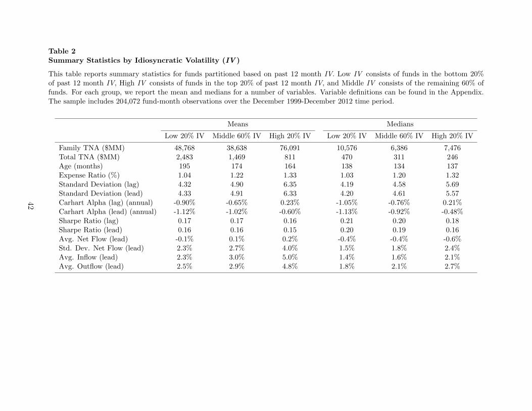
Table 2Summary Statistics by Idiosyncratic Volatility (IV )

This table reports summary statistics for funds partitioned based on past 12 month IV. Low IV consists of funds in the bottom 20%of past 12 month IV, High IV consists of funds in the top 20% of past 12 month IV, and Middle IV consists of the remaining 60% offunds. For each group, we report the mean and medians for a number of variables. Variable definitions can be found in the Appendix.The sample includes 204,072 fund-month observations over the December 1999-December 2012 time period.

Means Medians

Low 20% IV Middle 60% IV High 20% IV Low 20% IV Middle 60% IV High 20% IV

Family TNA ($MM) 48,768 38,638 76,091 10,576 6,386 7,476Total TNA ($MM) 2,483 1,469 811 470 311 246Age (months) 195 174 164 138 134 137Expense Ratio (%) 1.04 1.22 1.33 1.03 1.20 1.32Standard Deviation (lag) 4.32 4.90 6.35 4.19 4.58 5.69Standard Deviation (lead) 4.33 4.91 6.33 4.20 4.61 5.57Carhart Alpha (lag) (annual) -0.90% -0.65% 0.23% -1.05% -0.76% 0.21%Carhart Alpha (lead) (annual) -1.12% -1.02% -0.60% -1.13% -0.92% -0.48%Sharpe Ratio (lag) 0.17 0.17 0.16 0.21 0.20 0.18Sharpe Ratio (lead) 0.16 0.16 0.15 0.20 0.19 0.16Avg. Net Flow (lead) -0.1% 0.1% 0.2% -0.4% -0.4% -0.6%Std. Dev. Net Flow (lead) 2.3% 2.7% 4.0% 1.5% 1.8% 2.4%Avg. Inflow (lead) 2.3% 3.0% 5.0% 1.4% 1.6% 2.1%Avg. Outflow (lead) 2.5% 2.9% 4.8% 1.8% 2.1% 2.7%

42

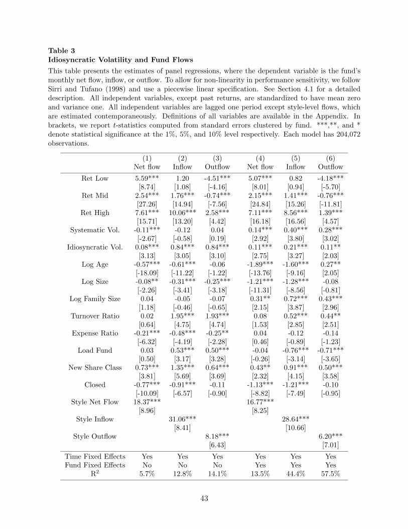
Table 3Idiosyncratic Volatility and Fund Flows

This table presents the estimates of panel regressions, where the dependent variable is the fund’smonthly net flow, inflow, or outflow. To allow for non-linearity in performance sensitivity, we followSirri and Tufano (1998) and use a piecewise linear specification. See Section 4.1 for a detaileddescription. All independent variables, except past returns, are standardized to have mean zeroand variance one. All independent variables are lagged one period except style-level flows, whichare estimated contemporaneously. Definitions of all variables are available in the Appendix. Inbrackets, we report t-statistics computed from standard errors clustered by fund. ***,**, and *denote statistical significance at the 1%, 5%, and 10% level respectively. Each model has 204,072observations.

(1) (2) (3) (4) (5) (6)Net flow Inflow Outflow Net flow Inflow Outflow

Ret Low 5.59*** 1.20 -4.51*** 5.07*** 0.82 -4.18***[8.74] [1.08] [-4.16] [8.01] [0.94] [-5.70]

Ret Mid 2.54*** 1.76*** -0.74*** 2.15*** 1.41*** -0.76***[27.26] [14.94] [-7.56] [24.84] [15.26] [-11.81]

Ret High 7.61*** 10.06*** 2.58*** 7.11*** 8.56*** 1.39***[15.71] [13.20] [4.42] [16.18] [16.56] [4.57]

Systematic Vol. -0.11*** -0.12 0.04 0.14*** 0.40*** 0.28***[-2.67] [-0.58] [0.19] [2.92] [3.80] [3.02]

Idiosyncratic Vol. 0.08*** 0.84*** 0.84*** 0.11*** 0.21*** 0.11**[3.13] [3.05] [3.10] [2.75] [3.27] [2.03]

Log Age -0.57*** -0.61*** -0.06 -1.89*** -1.60*** 0.27**[-18.09] [-11.22] [-1.22] [-13.76] [-9.16] [2.05]

Log Size -0.08** -0.31*** -0.25*** -1.21*** -1.28*** -0.08[-2.26] [-3.41] [-3.18] [-11.31] [-8.56] [-0.81]

Log Family Size 0.04 -0.05 -0.07 0.31** 0.72*** 0.43***[1.18] [-0.46] [-0.65] [2.15] [3.87] [2.96]

Turnover Ratio 0.02 1.95*** 1.93*** 0.08 0.52*** 0.44**[0.64] [4.75] [4.74] [1.53] [2.85] [2.51]

Expense Ratio -0.21*** -0.48*** -0.25** 0.04 -0.12 -0.14[-6.32] [-4.19] [-2.28] [0.46] [-0.89] [-1.23]

Load Fund 0.03 0.53*** 0.50*** -0.04 -0.76*** -0.71***[0.50] [3.17] [3.28] [-0.26] [-3.14] [-3.65]

New Share Class 0.73*** 1.35*** 0.64*** 0.43** 0.91*** 0.50***[3.81] [5.69] [3.69] [2.32] [4.15] [3.58]

Closed -0.77*** -0.91*** -0.11 -1.13*** -1.21*** -0.10[-10.09] [-6.57] [-0.90] [-8.82] [-7.49] [-0.95]

Style Net Flow 18.37*** 16.77***[8.96] [8.25]

Style Inflow 31.06*** 28.64***[8.41] [10.66]

Style Outflow 8.18*** 6.20***[6.43] [7.01]

Time Fixed Effects Yes Yes Yes Yes Yes YesFund Fixed Effects No No No Yes Yes Yes

R2 5.7% 12.8% 14.1% 13.5% 44.4% 57.5%

43

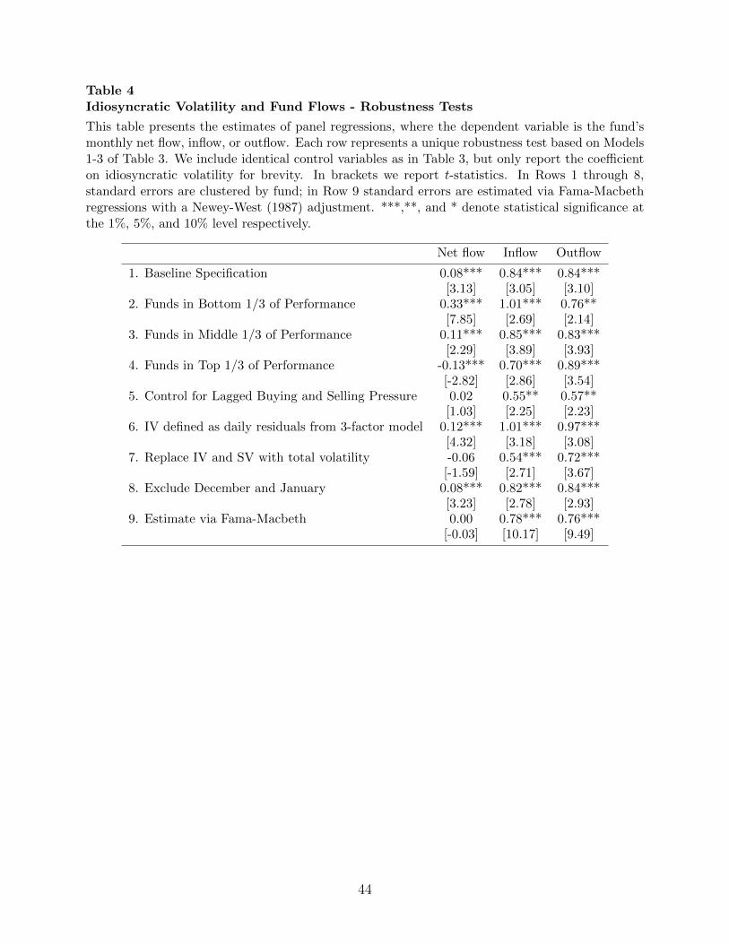
Table 4Idiosyncratic Volatility and Fund Flows - Robustness Tests

This table presents the estimates of panel regressions, where the dependent variable is the fund’smonthly net flow, inflow, or outflow. Each row represents a unique robustness test based on Models1-3 of Table 3. We include identical control variables as in Table 3, but only report the coefficienton idiosyncratic volatility for brevity. In brackets we report t-statistics. In Rows 1 through 8,standard errors are clustered by fund; in Row 9 standard errors are estimated via Fama-Macbethregressions with a Newey-West (1987) adjustment. ***,**, and * denote statistical significance atthe 1%, 5%, and 10% level respectively.

Net flow Inflow Outflow

1. Baseline Specification 0.08*** 0.84*** 0.84***[3.13] [3.05] [3.10]

2. Funds in Bottom 1/3 of Performance 0.33*** 1.01*** 0.76**[7.85] [2.69] [2.14]

3. Funds in Middle 1/3 of Performance 0.11*** 0.85*** 0.83***[2.29] [3.89] [3.93]

4. Funds in Top 1/3 of Performance -0.13*** 0.70*** 0.89***[-2.82] [2.86] [3.54]

5. Control for Lagged Buying and Selling Pressure 0.02 0.55** 0.57**[1.03] [2.25] [2.23]

6. IV defined as daily residuals from 3-factor model 0.12*** 1.01*** 0.97***[4.32] [3.18] [3.08]

7. Replace IV and SV with total volatility -0.06 0.54*** 0.72***[-1.59] [2.71] [3.67]

8. Exclude December and January 0.08*** 0.82*** 0.84***[3.23] [2.78] [2.93]

9. Estimate via Fama-Macbeth 0.00 0.78*** 0.76***[-0.03] [10.17] [9.49]

44

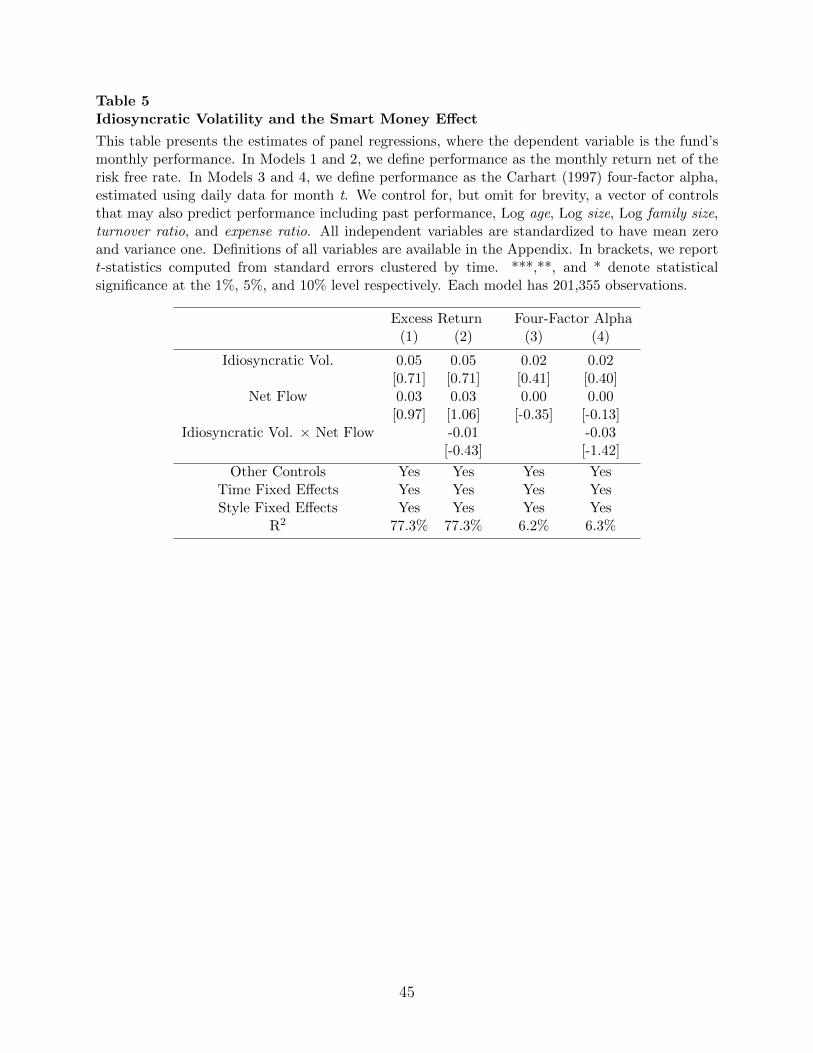
Table 5Idiosyncratic Volatility and the Smart Money Effect

This table presents the estimates of panel regressions, where the dependent variable is the fund’smonthly performance. In Models 1 and 2, we define performance as the monthly return net of therisk free rate. In Models 3 and 4, we define performance as the Carhart (1997) four-factor alpha,estimated using daily data for month t. We control for, but omit for brevity, a vector of controlsthat may also predict performance including past performance, Log age, Log size, Log family size,turnover ratio, and expense ratio. All independent variables are standardized to have mean zeroand variance one. Definitions of all variables are available in the Appendix. In brackets, we reportt-statistics computed from standard errors clustered by time. ***,**, and * denote statisticalsignificance at the 1%, 5%, and 10% level respectively. Each model has 201,355 observations.

Excess Return Four-Factor Alpha(1) (2) (3) (4)

Idiosyncratic Vol. 0.05 0.05 0.02 0.02[0.71] [0.71] [0.41] [0.40]

Net Flow 0.03 0.03 0.00 0.00[0.97] [1.06] [-0.35] [-0.13]

Idiosyncratic Vol. × Net Flow -0.01 -0.03[-0.43] [-1.42]

Other Controls Yes Yes Yes YesTime Fixed Effects Yes Yes Yes YesStyle Fixed Effects Yes Yes Yes Yes

R2 77.3% 77.3% 6.2% 6.3%

45

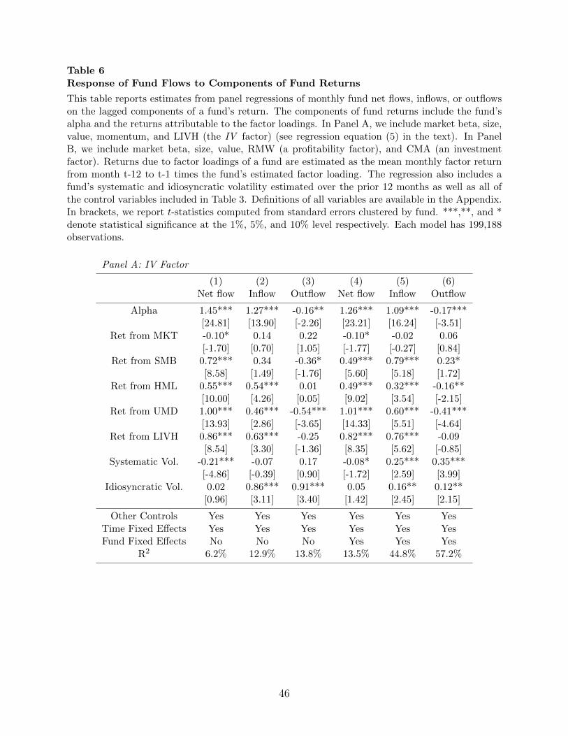
Table 6Response of Fund Flows to Components of Fund Returns

This table reports estimates from panel regressions of monthly fund net flows, inflows, or outflowson the lagged components of a fund’s return. The components of fund returns include the fund’salpha and the returns attributable to the factor loadings. In Panel A, we include market beta, size,value, momentum, and LIVH (the IV factor) (see regression equation (5) in the text). In PanelB, we include market beta, size, value, RMW (a profitability factor), and CMA (an investmentfactor). Returns due to factor loadings of a fund are estimated as the mean monthly factor returnfrom month t-12 to t-1 times the fund’s estimated factor loading. The regression also includes afund’s systematic and idiosyncratic volatility estimated over the prior 12 months as well as all ofthe control variables included in Table 3. Definitions of all variables are available in the Appendix.In brackets, we report t-statistics computed from standard errors clustered by fund. ***,**, and *denote statistical significance at the 1%, 5%, and 10% level respectively. Each model has 199,188observations.

Panel A: IV Factor

(1) (2) (3) (4) (5) (6)Net flow Inflow Outflow Net flow Inflow Outflow

Alpha 1.45*** 1.27*** -0.16** 1.26*** 1.09*** -0.17***[24.81] [13.90] [-2.26] [23.21] [16.24] [-3.51]

Ret from MKT -0.10* 0.14 0.22 -0.10* -0.02 0.06[-1.70] [0.70] [1.05] [-1.77] [-0.27] [0.84]

Ret from SMB 0.72*** 0.34 -0.36* 0.49*** 0.79*** 0.23*[8.58] [1.49] [-1.76] [5.60] [5.18] [1.72]

Ret from HML 0.55*** 0.54*** 0.01 0.49*** 0.32*** -0.16**[10.00] [4.26] [0.05] [9.02] [3.54] [-2.15]

Ret from UMD 1.00*** 0.46*** -0.54*** 1.01*** 0.60*** -0.41***[13.93] [2.86] [-3.65] [14.33] [5.51] [-4.64]

Ret from LIVH 0.86*** 0.63*** -0.25 0.82*** 0.76*** -0.09[8.54] [3.30] [-1.36] [8.35] [5.62] [-0.85]

Systematic Vol. -0.21*** -0.07 0.17 -0.08* 0.25*** 0.35***[-4.86] [-0.39] [0.90] [-1.72] [2.59] [3.99]

Idiosyncratic Vol. 0.02 0.86*** 0.91*** 0.05 0.16** 0.12**[0.96] [3.11] [3.40] [1.42] [2.45] [2.15]

Other Controls Yes Yes Yes Yes Yes YesTime Fixed Effects Yes Yes Yes Yes Yes YesFund Fixed Effects No No No Yes Yes Yes

R2 6.2% 12.9% 13.8% 13.5% 44.8% 57.2%

46

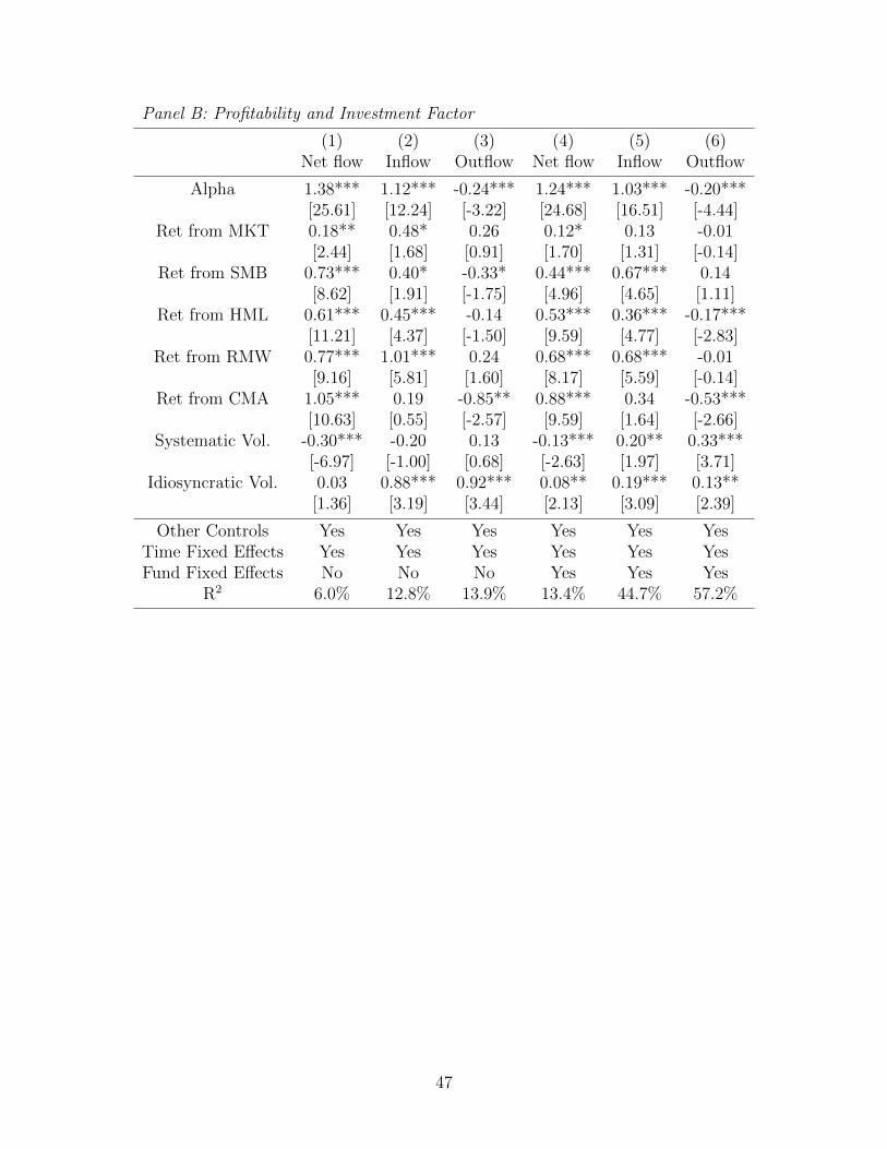
Panel B: Profitability and Investment Factor

(1) (2) (3) (4) (5) (6)Net flow Inflow Outflow Net flow Inflow Outflow

Alpha 1.38*** 1.12*** -0.24*** 1.24*** 1.03*** -0.20***[25.61] [12.24] [-3.22] [24.68] [16.51] [-4.44]

Ret from MKT 0.18** 0.48* 0.26 0.12* 0.13 -0.01[2.44] [1.68] [0.91] [1.70] [1.31] [-0.14]

Ret from SMB 0.73*** 0.40* -0.33* 0.44*** 0.67*** 0.14[8.62] [1.91] [-1.75] [4.96] [4.65] [1.11]

Ret from HML 0.61*** 0.45*** -0.14 0.53*** 0.36*** -0.17***[11.21] [4.37] [-1.50] [9.59] [4.77] [-2.83]

Ret from RMW 0.77*** 1.01*** 0.24 0.68*** 0.68*** -0.01[9.16] [5.81] [1.60] [8.17] [5.59] [-0.14]

Ret from CMA 1.05*** 0.19 -0.85** 0.88*** 0.34 -0.53***[10.63] [0.55] [-2.57] [9.59] [1.64] [-2.66]

Systematic Vol. -0.30*** -0.20 0.13 -0.13*** 0.20** 0.33***[-6.97] [-1.00] [0.68] [-2.63] [1.97] [3.71]

Idiosyncratic Vol. 0.03 0.88*** 0.92*** 0.08** 0.19*** 0.13**[1.36] [3.19] [3.44] [2.13] [3.09] [2.39]

Other Controls Yes Yes Yes Yes Yes YesTime Fixed Effects Yes Yes Yes Yes Yes YesFund Fixed Effects No No No Yes Yes Yes

R2 6.0% 12.8% 13.9% 13.4% 44.7% 57.2%

47

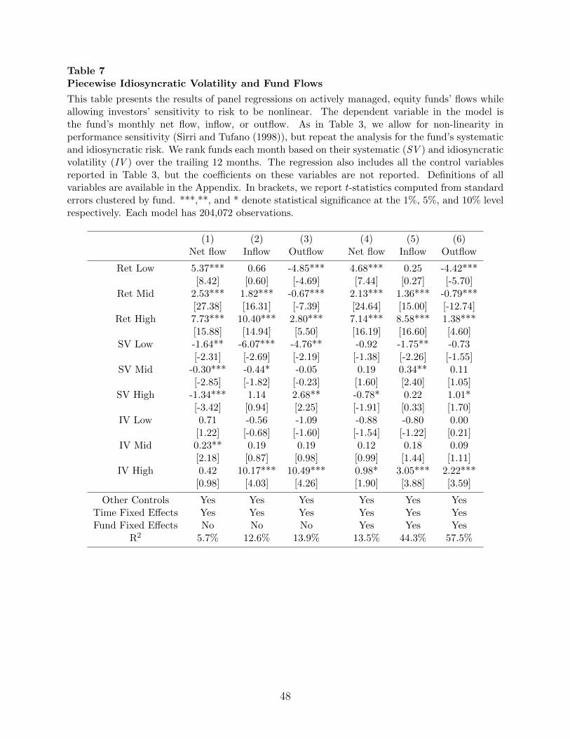
Table 7Piecewise Idiosyncratic Volatility and Fund Flows

This table presents the results of panel regressions on actively managed, equity funds’ flows whileallowing investors’ sensitivity to risk to be nonlinear. The dependent variable in the model isthe fund’s monthly net flow, inflow, or outflow. As in Table 3, we allow for non-linearity inperformance sensitivity (Sirri and Tufano (1998)), but repeat the analysis for the fund’s systematicand idiosyncratic risk. We rank funds each month based on their systematic (SV ) and idiosyncraticvolatility (IV ) over the trailing 12 months. The regression also includes all the control variablesreported in Table 3, but the coefficients on these variables are not reported. Definitions of allvariables are available in the Appendix. In brackets, we report t-statistics computed from standarderrors clustered by fund. ***,**, and * denote statistical significance at the 1%, 5%, and 10% levelrespectively. Each model has 204,072 observations.

(1) (2) (3) (4) (5) (6)Net flow Inflow Outflow Net flow Inflow Outflow

Ret Low 5.37*** 0.66 -4.85*** 4.68*** 0.25 -4.42***[8.42] [0.60] [-4.69] [7.44] [0.27] [-5.70]

Ret Mid 2.53*** 1.82*** -0.67*** 2.13*** 1.36*** -0.79***[27.38] [16.31] [-7.39] [24.64] [15.00] [-12.74]

Ret High 7.73*** 10.40*** 2.80*** 7.14*** 8.58*** 1.38***[15.88] [14.94] [5.50] [16.19] [16.60] [4.60]

SV Low -1.64** -6.07*** -4.76** -0.92 -1.75** -0.73[-2.31] [-2.69] [-2.19] [-1.38] [-2.26] [-1.55]

SV Mid -0.30*** -0.44* -0.05 0.19 0.34** 0.11[-2.85] [-1.82] [-0.23] [1.60] [2.40] [1.05]

SV High -1.34*** 1.14 2.68** -0.78* 0.22 1.01*[-3.42] [0.94] [2.25] [-1.91] [0.33] [1.70]

IV Low 0.71 -0.56 -1.09 -0.88 -0.80 0.00[1.22] [-0.68] [-1.60] [-1.54] [-1.22] [0.21]

IV Mid 0.23** 0.19 0.19 0.12 0.18 0.09[2.18] [0.87] [0.98] [0.99] [1.44] [1.11]

IV High 0.42 10.17*** 10.49*** 0.98* 3.05*** 2.22***[0.98] [4.03] [4.26] [1.90] [3.88] [3.59]

Other Controls Yes Yes Yes Yes Yes YesTime Fixed Effects Yes Yes Yes Yes Yes YesFund Fixed Effects No No No Yes Yes Yes

R2 5.7% 12.6% 13.9% 13.5% 44.3% 57.5%

48

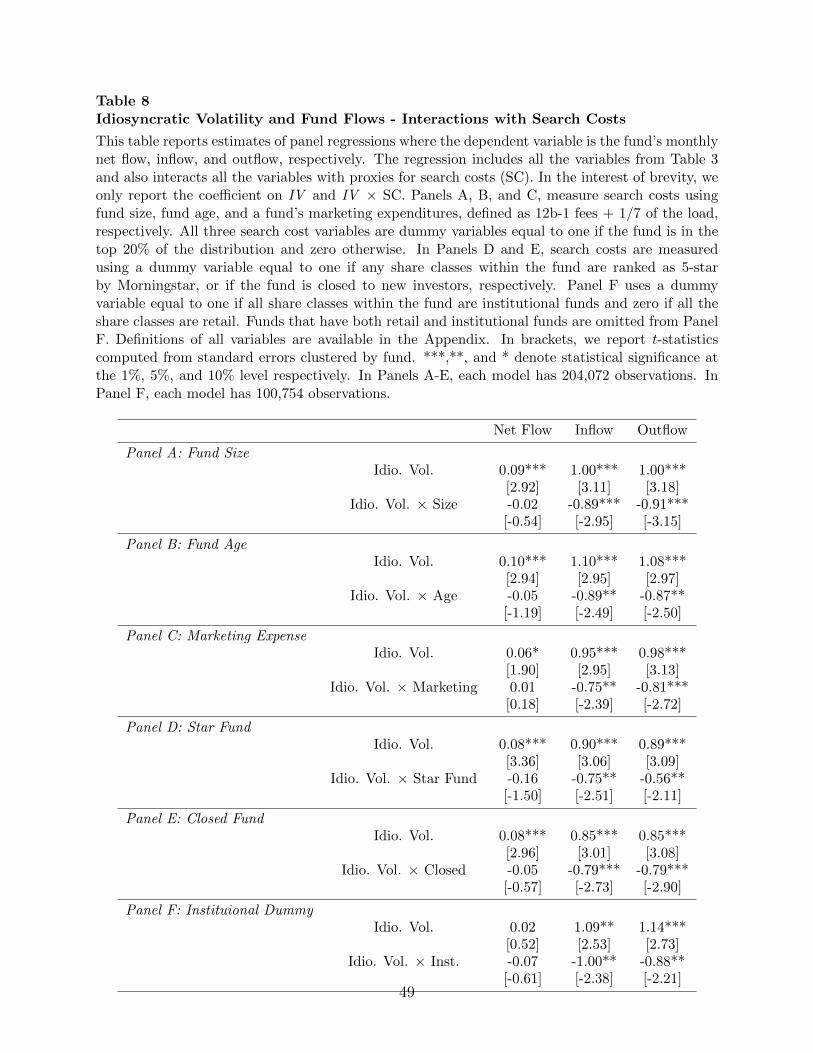
Table 8Idiosyncratic Volatility and Fund Flows - Interactions with Search Costs

This table reports estimates of panel regressions where the dependent variable is the fund’s monthlynet flow, inflow, and outflow, respectively. The regression includes all the variables from Table 3and also interacts all the variables with proxies for search costs (SC). In the interest of brevity, weonly report the coefficient on IV and IV × SC. Panels A, B, and C, measure search costs usingfund size, fund age, and a fund’s marketing expenditures, defined as 12b-1 fees + 1/7 of the load,respectively. All three search cost variables are dummy variables equal to one if the fund is in thetop 20% of the distribution and zero otherwise. In Panels D and E, search costs are measuredusing a dummy variable equal to one if any share classes within the fund are ranked as 5-starby Morningstar, or if the fund is closed to new investors, respectively. Panel F uses a dummyvariable equal to one if all share classes within the fund are institutional funds and zero if all theshare classes are retail. Funds that have both retail and institutional funds are omitted from PanelF. Definitions of all variables are available in the Appendix. In brackets, we report t-statisticscomputed from standard errors clustered by fund. ***,**, and * denote statistical significance atthe 1%, 5%, and 10% level respectively. In Panels A-E, each model has 204,072 observations. InPanel F, each model has 100,754 observations.

Net Flow Inflow Outflow

Panel A: Fund SizeIdio. Vol. 0.09*** 1.00*** 1.00***

[2.92] [3.11] [3.18]Idio. Vol. × Size -0.02 -0.89*** -0.91***

[-0.54] [-2.95] [-3.15]

Panel B: Fund AgeIdio. Vol. 0.10*** 1.10*** 1.08***

[2.94] [2.95] [2.97]Idio. Vol. × Age -0.05 -0.89** -0.87**

[-1.19] [-2.49] [-2.50]

Panel C: Marketing ExpenseIdio. Vol. 0.06* 0.95*** 0.98***

[1.90] [2.95] [3.13]Idio. Vol. × Marketing 0.01 -0.75** -0.81***

[0.18] [-2.39] [-2.72]

Panel D: Star FundIdio. Vol. 0.08*** 0.90*** 0.89***

[3.36] [3.06] [3.09]Idio. Vol. × Star Fund -0.16 -0.75** -0.56**

[-1.50] [-2.51] [-2.11]

Panel E: Closed FundIdio. Vol. 0.08*** 0.85*** 0.85***

[2.96] [3.01] [3.08]Idio. Vol. × Closed -0.05 -0.79*** -0.79***

[-0.57] [-2.73] [-2.90]

Panel F: Instituional DummyIdio. Vol. 0.02 1.09** 1.14***

[0.52] [2.53] [2.73]Idio. Vol. × Inst. -0.07 -1.00** -0.88**

[-0.61] [-2.38] [-2.21]49

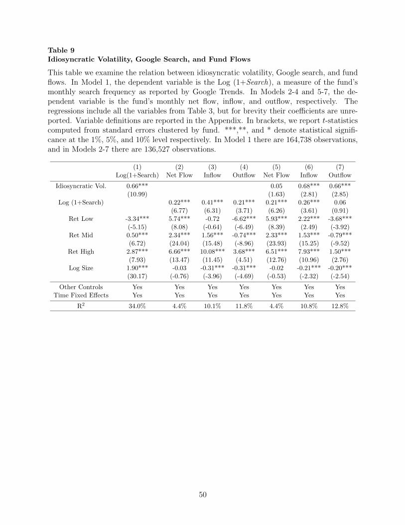
Table 9Idiosyncratic Volatility, Google Search, and Fund Flows

This table we examine the relation between idiosyncratic volatility, Google search, and fundflows. In Model 1, the dependent variable is the Log (1+Search), a measure of the fund’smonthly search frequency as reported by Google Trends. In Models 2-4 and 5-7, the de-pendent variable is the fund’s monthly net flow, inflow, and outflow, respectively. Theregressions include all the variables from Table 3, but for brevity their coefficients are unre-ported. Variable definitions are reported in the Appendix. In brackets, we report t-statisticscomputed from standard errors clustered by fund. ***,**, and * denote statistical signifi-cance at the 1%, 5%, and 10% level respectively. In Model 1 there are 164,738 observations,and in Models 2-7 there are 136,527 observations.

(1) (2) (3) (4) (5) (6) (7)Log(1+Search) Net Flow Inflow Outflow Net Flow Inflow Outflow

Idiosyncratic Vol. 0.66*** 0.05 0.68*** 0.66***(10.99) (1.63) (2.81) (2.85)

Log (1+Search) 0.22*** 0.41*** 0.21*** 0.21*** 0.26*** 0.06(6.77) (6.31) (3.71) (6.26) (3.61) (0.91)

Ret Low -3.34*** 5.74*** -0.72 -6.62*** 5.93*** 2.22*** -3.68***(-5.15) (8.08) (-0.64) (-6.49) (8.39) (2.49) (-3.92)

Ret Mid 0.50*** 2.34*** 1.56*** -0.74*** 2.33*** 1.53*** -0.79***(6.72) (24.04) (15.48) (-8.96) (23.93) (15.25) (-9.52)

Ret High 2.87*** 6.66*** 10.08*** 3.68*** 6.51*** 7.93*** 1.50***(7.93) (13.47) (11.45) (4.51) (12.76) (10.96) (2.76)

Log Size 1.90*** -0.03 -0.31*** -0.31*** -0.02 -0.21*** -0.20***(30.17) (-0.76) (-3.96) (-4.69) (-0.53) (-2.32) (-2.54)

Other Controls Yes Yes Yes Yes Yes Yes YesTime Fixed Effects Yes Yes Yes Yes Yes Yes Yes

R2 34.0% 4.4% 10.1% 11.8% 4.4% 10.8% 12.8%

50

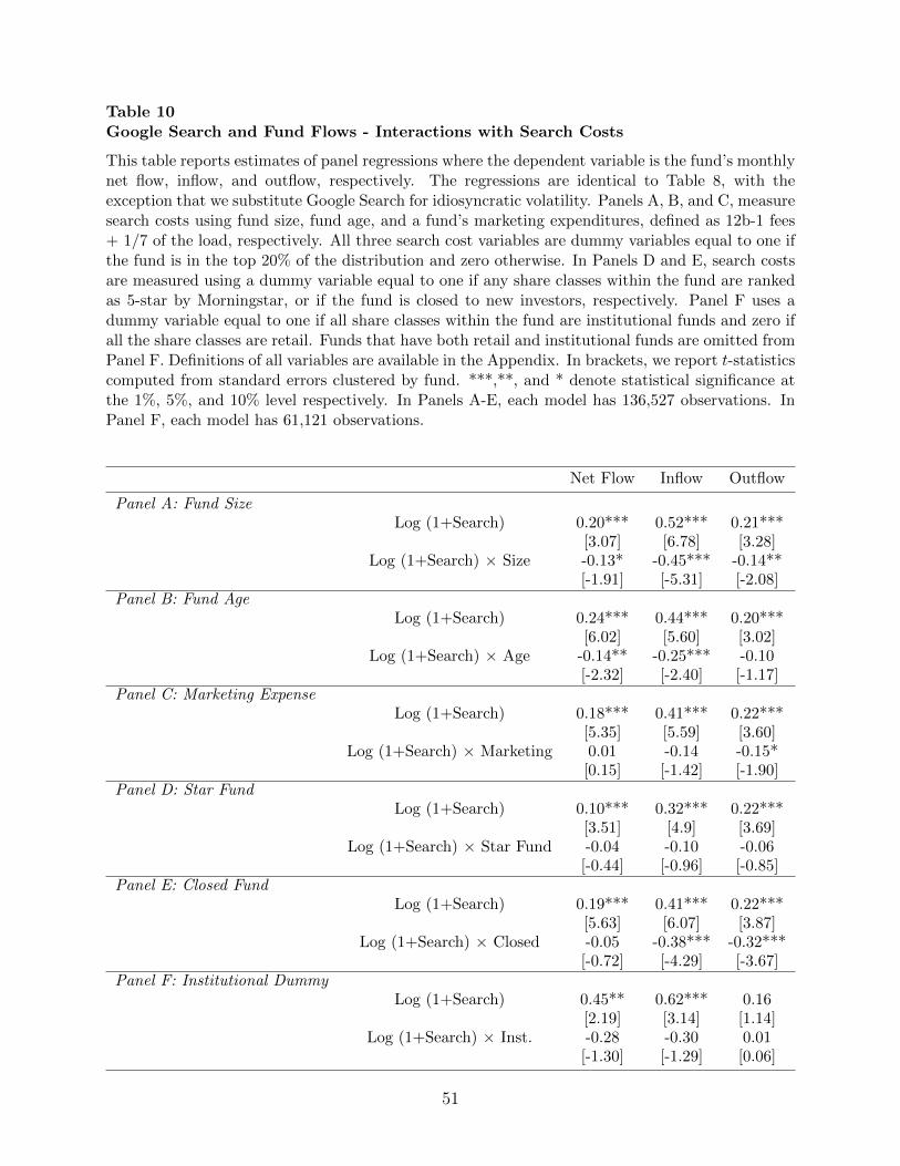
Table 10Google Search and Fund Flows - Interactions with Search Costs

This table reports estimates of panel regressions where the dependent variable is the fund’s monthlynet flow, inflow, and outflow, respectively. The regressions are identical to Table 8, with theexception that we substitute Google Search for idiosyncratic volatility. Panels A, B, and C, measuresearch costs using fund size, fund age, and a fund’s marketing expenditures, defined as 12b-1 fees+ 1/7 of the load, respectively. All three search cost variables are dummy variables equal to one ifthe fund is in the top 20% of the distribution and zero otherwise. In Panels D and E, search costsare measured using a dummy variable equal to one if any share classes within the fund are rankedas 5-star by Morningstar, or if the fund is closed to new investors, respectively. Panel F uses adummy variable equal to one if all share classes within the fund are institutional funds and zero ifall the share classes are retail. Funds that have both retail and institutional funds are omitted fromPanel F. Definitions of all variables are available in the Appendix. In brackets, we report t-statisticscomputed from standard errors clustered by fund. ***,**, and * denote statistical significance atthe 1%, 5%, and 10% level respectively. In Panels A-E, each model has 136,527 observations. InPanel F, each model has 61,121 observations.

Net Flow Inflow Outflow

Panel A: Fund SizeLog (1+Search) 0.20*** 0.52*** 0.21***

[3.07] [6.78] [3.28]Log (1+Search) × Size -0.13* -0.45*** -0.14**

[-1.91] [-5.31] [-2.08]Panel B: Fund Age

Log (1+Search) 0.24*** 0.44*** 0.20***[6.02] [5.60] [3.02]

Log (1+Search) × Age -0.14** -0.25*** -0.10[-2.32] [-2.40] [-1.17]

Panel C: Marketing ExpenseLog (1+Search) 0.18*** 0.41*** 0.22***

[5.35] [5.59] [3.60]Log (1+Search) × Marketing 0.01 -0.14 -0.15*

[0.15] [-1.42] [-1.90]Panel D: Star Fund

Log (1+Search) 0.10*** 0.32*** 0.22***[3.51] [4.9] [3.69]

Log (1+Search) × Star Fund -0.04 -0.10 -0.06[-0.44] [-0.96] [-0.85]

Panel E: Closed FundLog (1+Search) 0.19*** 0.41*** 0.22***

[5.63] [6.07] [3.87]Log (1+Search) × Closed -0.05 -0.38*** -0.32***

[-0.72] [-4.29] [-3.67]Panel F: Institutional Dummy

Log (1+Search) 0.45** 0.62*** 0.16[2.19] [3.14] [1.14]

Log (1+Search) × Inst. -0.28 -0.30 0.01[-1.30] [-1.29] [0.06]

51