Non-Parametric Estimation of SearchCosts for Differentiated Products:

Evidence from Medigap∗

Haizhen Lin†

Matthijs R. Wildenbeest‡

January 2019

Abstract

This paper develops a method to estimate search frictions as well as preferenceparameters in differentiated product markets. Search costs are non-parametricallyidentified, which means our method can be used to estimate search costs in differen-tiated product markets that lack a suitable search cost shifter. We apply our modelto the U.S. Medigap insurance market. We find that search costs are substantial:the estimated median cost of searching for an insurer is $30. Using the estimatedparameters we find that eliminating search costs could result in price decreases of asmuch as $71 (or 4.7 percent), along with increases in average consumer welfare of upto $374.

Keywords: price dispersion, consumer search, product differentiation, health insurance

JEL Classification: I13, D83, L15

∗We are grateful to the Editor, an Associate Editor, and two anonymous referees for their very usefulcomments and suggestions. In addition we thank Mike Baye, Kate Bundorf, Andrew Ching, Leemore Dafny,David Dranove, Hanming Fang, Marty Gaynor, Lorens Helmchen, Claudio Lucarelli, Nicole Maestas, JeffPrince, Jon Skinner, Kosali Simon, Alan Sorensen, and participants at various seminars and conferencesfor helpful comments and suggestions. This paper was previously circulated under the title “Search andPrices in the Medigap Insurance Market.”†Indiana University, Kelley School of Business and NBER, E-mail: hzlin@indiana.edu.‡Indiana University, Kelley School of Business, E-mail: mwildenb@indiana.edu (corresponding author).

1

1 Introduction

Since Stigler’s seminal article on the economics of information, economists have tried to

relate price dispersion to search frictions: if it is costly for consumers to obtain price

information, because, for instance, finding out prices means visiting sellers or making phone

calls, some will choose not to compare prices. As a result some firms might set high prices to

maximize profits from those who do not compare price offers, and others might set relatively

low prices to maximize surplus from price comparers, resulting in price dispersion.

An additional explanation for price variation is product differentiation. Even in settings

in which a specific product is essentially a homogeneous good, firms might differ in terms

of quality or service-related characteristics, such as branding and service quality, allowing

higher-quality firms to charge higher prices. Product differentiation and search can also go

together: as shown by Wolinsky (1986) and Anderson and Renault (1999), if consumers

search not only for low prices, but also for horizontal characteristics such as whether the

product is a good fit, equilibrium prices rise with search costs.

The objective of this paper is to develop a model of search and product differentiation

that allows us to non-parametrically identify the contributions of search frictions and prod-

uct differentiation in explaining price dispersion. In Section 2 of the paper we present a

model in which consumers search for products that are horizontally and vertically differ-

entiated. Consumers determine before they search which firms to contact for information

about products and prices; they do so by making a trade-off between the expected utility

of contacting a subset of firms and the corresponding search costs.

We show how to estimate the model using aggregate data on prices, market shares,

and product characteristics. An attractive feature of our model is that search costs are

non-parametrically identified, i.e., we do not have to make any specific assumptions about

the distribution of search costs. Under the assumption that consumers are homogeneous in

how they value observed characteristics (i.e., we cannot allow for random coefficients), we

separately identify search costs without using additional data on search behavior or search

cost shifters, which are often not available to researchers.

In Section 3 we use the model to study price dispersion in the U.S. Medigap insurance

market. Medigap is a form of private insurance designed to supplement Medicare by filling

2

in coverage gaps in Medicare payments. One important feature of the Medigap market is

plan standardization, meaning that within a given plan type, the same set of benefits and

coverage needs to be offered, regardless of which insurer sells the plan. Irrespective of plan

standardization, we observe substantial price variation across insurers within a market (with

an average coefficient of variation larger than 0.2 in most cases), which we define at the

state level. In explaining observed price variation, we first present reduced-form evidence

that suggests both product differentiation and search frictions play important roles. We

then estimate our search model using aggregate data on prices and market shares.

Our estimates indicate that search costs are substantial: the estimated median search

cost is $30 per search. There is also large variation in search costs across the population.

In our counterfactuals, we study the competitive effects of lowering search costs. Assuming

firms set prices to maximize profits, we determine to what extent prices would change if

quotes are obtained at no cost. According to our simulations, weighted average prices

decrease by $71, which is 4.7 percent of the average yearly policy premium. Consumer

welfare, which includes savings on search costs as well as the expansion of the market,

increases by up to $374 on average if search costs are zero.

Our main contribution is to develop a framework that allows for non-parametric identi-

fication of search costs in settings in which product differentiation is important. In Section

4 of the paper we use Monte Carlo experiments to show that our estimation method is

indeed capable of recovering preference parameters as well as the search cost distribution,

without having to make any parametric assumptions on the search cost distribution. We

also study the performance of our model when the data is generated using a richer frame-

work in which consumers have heterogenous preferences for observed characteristics (as in

Moraga-Gonzalez et al., 2015). An important difference is that search costs are consumer-

specific in our model, whereas Moraga-Gonzalez et al. (2015) add a consumer-choice-set

specific search cost shock to keep estimation of their model tractable. We find that our

model does reasonably well when the variance of the choice-set specific search cost shock

is small.

3

Related literature

Our paper is part of the consumer search literature. Within this literature, several papers

have studied search behavior in insurance markets. Brown and Goolsbee (2002) show that

reduced search costs, resulting from increased usage of Internet price comparison sites, lead

to lower prices for term life policies. Cebul et al. (2011) find that search frictions in private

health insurance markets lead to high prices and price dispersion, excessive marketing costs,

and high insurance turnover. They also suggest that government-financed public insurance

can reduce distortions created by search frictions. In other settings, Hortacsu and Syverson

(2004) build a model of product differentiation and search, and find that both are important

determinants of fee dispersion in the retail S&P 500 index funds sector. Wildenbeest (2011)

provides a framework for studying price dispersion in markets with product differentiation

and search frictions and shows how to estimate search costs using only price data. These

two papers allow for non-parametric identification of the search cost distribution, as in

our model. However, consumers search for vertically differentiated firms in Hortacsu and

Syverson (2004) and Wildenbeest (2011), whereas firms are both horizontally and vertically

differentiated in our model. Moreover, in these models consumers search randomly, whereas

search is directed in our model. Directed search, or ordered search, is typically thought of

as a natural way to search in markets in which certain firms are more prominent than others

(see Armstrong, 2017, for a discussion of the theoretical literature on ordered search).

Our paper most closely relates to a study by Moraga-Gonzalez et al. (2015), who add

search to the demand estimation framework of Berry et al. (1995). Moraga-Gonzalez et al.

(2015) study the Dutch automobile market. To be able to separately identify heterogene-

ity in search costs from heterogeneity in preference parameters, they link search costs to

distances between consumers and dealer locations. Our model builds on their findings;

however, by working in a conditional logit rather than a mixed logit framework, we allow

search costs to be non-parametrically identified, which is useful if the data lacks a suitable

search cost shifter. We discuss differences between our model and theirs in more detail in

Section 4.

Our paper also fits into the literature that studies Medigap prices and price dispersion.

Robst (2006) adopts a hedonic pricing model in order to examine the determinants of

4

Medigap premiums. Our paper is closely related to Maestas et al. (2009), who use the

search model of Carlson and McAfee (1983) to model price dispersion for Medigap plans.

They find that the average search cost in this market is $72. Unlike Maestas et al. (2009),

we model the joint decision of which plan type to obtain and which insurer to choose. To

allow for differences in plan-type preferences, our utility specification includes a stochastic

utility shock, which we model as ex-ante unobserved by the decision maker. As a result,

in our model consumers search for prices as well as a good fit in terms of insurer and plan

type. A second difference is that search is random in their model, while in our model

search is directed. In our model, consumers rank insurers according to the expected utility,

and depending on the decision-maker’s search costs, contact an optimal set of the highest-

ranked insurers to obtain information about prices and plan-type matches. In differentiated

product markets in which consumers have some prior information on the characteristics of

the firms, the optimal way to search is to start with the alternative that provides the highest

expected utility (see, for instance, Weitzman, 1979; Chade and Smith, 2006). In Maestas

et al. (2009) consumers have no prior information on the expected utility; therefore all

alternatives are ex-ante similar and consumers search randomly. In a random search model

lower ranked firms are as likely to be part of a consumer’s choice set as higher ranked firms,

whereas in our directed search model a consumer needs to have low search costs to sample

a lower ranked firm. To explain demand at lower ranked firms search costs therefore have

to be lower in our directed search model than in the random search model. Finally, whereas

Maestas et al. (2009) assume that search costs are uniformly distributed, our model does

not require any assumptions on the shape of the search cost distribution, which can be an

advantage if one does not know a priori what the search cost distribution looks like.

2 Model

In this section we develop a theoretical and empirical framework that takes search and

product differentiation as its main ingredients. As in Anderson and Renault (1999) and

Wolinsky (1986), our model also allows for horizontal product differentiation in order to

capture uncertainty concerning which products offered by a firm are best suited for an

individual. This means that in our model consumers search to find out price information

5

as well as which of the products offered by the competing firms is a good match.

2.1 Optimal Consumer Search

Consumer i derives utility from consumption of a product j ∈ {1, 2, . . . , J} sold by firm

f ∈ {1, 2, . . . , F} according to:

uijf = x′jfβ − αpjf + ξjf + εijf = δjf + εijf ,

where xjf are characteristics observed by both the researcher and the consumer, ξjf is a

vertical characteristic observed by the consumer only, and εijf is a matching term unob-

served by both the researcher and the consumer, which follows a standard Type I Extreme

Value distribution. The mean utility of product j sold by firm f is given by δjf . The utility

of not buying any of the products is ui0 = εi0.

We assume that consumers search nonsequentially. Consumers have information about

xjf and ξjf , but not about matching parameters εijf and prices pjf , and they have to visit

firms to discover these parameters. Search happens at the firm level, i.e., by visiting a firm

f the matching parameters and prices of all products sold by this firm are revealed. We

believe it is more natural to model search as first deciding on which firms to search for, and

then deciding which product to purchase. For instance, to get more information consumers

typically have to contact a firm, which means that search costs tend to occur at the firm

level and to a lesser extent at the product level (contacting a firm would allow consumers to

obtain information on all products sold by the firm). Search costs are consumer specific and

randomly distributed in [0,∞) according to the cumulative distribution function (CDF)

G(c).

Since consumers do not know the realization of εijf and pjf before they search, they

rank firms according to φf , where φf is the expected maximum utility of the set of products

Gf offered by firm f , i.e.,

φf = E

[maxj∈Gf{uijf}

]= log

∑j∈Gf

eδjf

.

Here we have left out the Euler constant, since it is common to all firms and therefore

does not affect choices. Note that we use the standard assumption in the theoretical litera-

6

ture on search for differentiated products that consumers form rational expectations about

prices (as in Wolinsky, 1986; Anderson and Renault, 1999). This means that even though

consumers do not observe realized prices before searching, they use expected (equilibrium)

prices to rank firms.

Since the ranking is ex-ante the same for all consumers, we can index firms by their

expected maximum utility φf , i.e, firm f = 1 is the most attractive firm, firm f = 2

the second-most attractive, and so on. We assume consumers do not observe εi0 before

searching so they will not condition their search behavior on the utility of the outside option.

Should the utility of the outside option be observed before searching, search decisions would

have to be conditional on the utility of the outside option, which would greatly complicate

the analysis. Furthermore, we assume that the first observation is free, so that all consumers

will search at least once. This assumption, which is standard in the literature, is made to

assure that everyone in the market participates.

An individual consumer with search cost c chooses the number of firms to sample,

denoted k∗(c), to maximize her expected utility. That is,

k∗(c) = arg maxk{E[max{uij1, uij2, . . . , uijk}]− (k − 1)c},

where (k − 1) reflects that the first observation is obtained for free. As shown by Moraga-

Gonzalez et al. (2015), the assumption that εijf follows a Type I Extreme Value distribution

allows us to write the optimal number of quotes to obtain as

k∗(c) = arg maxk

{log

(1 +

k∑f=1

eφf

)− (k − 1)c

}.

We define c1 as the search cost of the consumer who is indifferent to obtaining quotes

from one or two firms, i.e., log(1 + eφ1) = log(1 + eφ1 + eφ2) − c1. Solving for c1 gives

c1 = log(1 + eφ2/(1 + eφ1)

). More generally, we define ck as the search cost of the consumer

who is indifferent regarding whether to search k or k + 1 times, i.e., log(

1 +∑k

f=1 eφf

)−

(k − 1)ck = log(

1 +∑k+1

f=1 eφf

)− kck. Solving for ck gives

ck = log

(1 +

eφk+1

1 +∑k

f=1 eφf

). (1)

Note that by definition φk is decreasing in k, which means that ck is decreasing in k as well.

Moreover, the above equation shows that critical search cost values cannot be negative.

7

Using the critical search cost values ck and the search cost distribution G(c), we can

calculate the fraction of individuals searching k times:

µ1 = 1−G(c1); (2a)

µk = G(ck−1)−G(ck), k = 2, . . . , N − 1; (2b)

µN = G(cN−1). (2c)

2.2 Consumer Demand

We now move to the discussion of aggregate demand. First consider product j sold by the

highest-ranked firm (i.e., the firm with the highest mean utility φf ). Since all consumers

visit this firm, the market share of product j is given by

sj1 =eδj1

1 + eφ1· µ1 +

eδj1

1 +∑2

`=1 eφ`· µ2 + . . .+

eδj1

1 +∑N

`=1 eφ`· µN =

N∑k=1

eδj1

1 +∑k

`=1 eφ`· µk.

The second-highest-ranked firm will only attract consumers who search at least twice,

whereas the third-highest-ranked firm will only attract consumers who search at least three

times. More generally, the market share of product j sold by the fth-highest-ranked firm

is

sjf =N∑k=f

eδjf

1 +∑k

`=1 eφ`· µk.

Using the market share of the outside good, i.e.,

s0 =N∑k=1

1

1 +∑k

`=1 eφ`· µk,

we can rewrite sj1 as sj1 = s0 ·eδj1 , or, by taking logs and rearranging, log sj1− log s0 = δj1.

Notice that the relation between the market share of the outside option and the market

share for a product sold by the highest-ranked firm is the same as in a standard demand

model with no search frictions. This is because we assume the first search is free, so

by construction all consumers search the highest-ranked firm. However, market share

expressions for lower-ranked firms will be different since we need to take into account that

because of search frictions, these firms will not be searched by all consumers. For example,

8

using the definition of s0, we can rewrite the market share for a product sold by the second-

highest-ranked firm sj2 as sj2 =(s0 − µ1/(1 + eφ1)

)· eδj2 . Since the overall market share of

the highest-ranked firm is s1 = s0 ·eφ1 , we can rewrite sj2 as sj2 = s0 (1− µ1/(s0 + s1))·eδj2 .

Taking logs and rearranging gives log sj2 − log s0 = δj2 + log (1− µ1/(s0 + s1)). More

generally, the difference between the log market share of product j sold by the fth-highest-

ranked firm and the log market share of the outside good can be written as

log sjf − log s0 = δjf +

f−1∑k=1

log

(1− µk

s0 +∑k

`=1 s` −∑k

`=2 µ`−1

). (3)

2.3 Estimation

We use equation (3) to estimate the model in the following way:

log sjf − log s0 = βXjf − αpj + γ1Rf1 + γ2Rf2 + . . .+ γN−1RfN−1 + ξj, (4)

where Rfk is a firm ranking-related dummy that is given by

Rfk =

1 if rankf > k;

0 if rankf ≤ k,

and

γk = log

(1− µk

/(s0 +

k∑`=1

s` −k∑`=2

µ`−1

)).

The estimated γk’s can be used to back out the µk’s, which represent the shares of consumers

searching k times. Specifically, solving for µk gives

µk = [1− eγk ]

(s0 +

k∑`=1

s` −k∑`=2

µ`−1

).

The µk’s can be obtained iteratively by starting with µ1: to calculate µ1 only γ1, s0, and s1

are needed; to calculate µ2, we can use the estimate of µ1, as well as γ2, s0, s1, and s2. To

derive a non-parametric estimate of the search cost distribution, we combine the estimates

of the µk’s with estimates of the search cost cutoffs ck. For this we use equation (1) as

well as estimates of the firm-specific logit inclusive value φf . The µk’s can then be mapped

into the quantiles of the search cost distribution that correspond to the search cost cutoff

values by inverting equations (2a)–(2c).

9

Note that by construction φ2 cannot be larger than φ1, so the minimum value of γ1

is log s2 − log s1, while the maximum value is 0. Similarly, the minimum value of γ2 is

log s3 − log s2, while the maximum value is again 0. This means that we can estimate

equation (4) using the constraint γk ∈ [log sk+1 − log sk, 0]. Note that this is equivalent

to estimating log sjf − log s0 = βXjf − αpj +∑f−1

k=1 γ′k(log sk+1 − log sk) + ξj using the

constraint γ′k ∈ [0, 1], where γk ≡ γ′k(log sk+1− log sk). In order to correct for the potential

endogeneity of prices, we construct two instrumental variables in the spirit of Hausman

(1996) and Nevo (2000). The first instrument is the average price of the same product

offered by the firm in other markets. The second is the average price of all products offered

by the firm in other markets. The identifying assumption is that market-specific valuations

are independent across markets.

Note that the ranking-related dummies are market and firm specific. In carrying out

our estimation, we pool firms ranked below a certain threshold for the purpose of restricting

the total number of these dummies. For example, in our application, we estimate a model

in which consumers can either search any number from one to four, or they search five

or more times, which allows them to obtain information on all the firms in the market.

Our estimation imposes an implicit assumption that consumers either have relatively high

search costs, such that they explicitly decide how many firms to search (up to four), or

that they have relatively low search costs, such that they obtain information on all firms

in the market.

2.4 Identification

We discuss identification of the parameters of the utility function, which are given by α and

β, as well as the parameters that reflect the search part of the model, which are given by

the vector of ranking-related parameters γ. Variation in product and firm characteristics

together with variation in market share allows us to identify the α and β parameters of the

utility function. To better explain how search costs parameters γ are separately identified,

let us consider two similar products sold by two different firms, with one firm being more

desirable than the other. In a full information model, these two products would have very

similar market shares. However, in a search model, the more desirable firm will be ranked

10

higher and therefore visited by more consumers, which gives its product an additional boost

in market share. As a result, differences in market shares of similar products offered by

different firms would allow us to identify the search cost parameters γ. As search costs

increase, market shares of products offered by the more popular firm will increase relative

to products offered by the less popular firm.

The discussion above assumes we use observed firm characteristics to capture firm het-

erogeneity. If we allow for firm fixed effects instead, separately identifying the effects of

firm differentiation from the effects of search frictions is more challenging. This is because

our model allows search cost parameters γ to vary across markets. In this case, separately

identifying firm fixed effects from search cost parameters requires observing multiple firms

that share the “same” ranking in a given market. In principle, this can be achieved in two

ways. First, because of the way the model is set up, firm fixed effects can be identified using

variation in identities of the highest-ranked firms across markets (and time). Identification

works here by taking advantage of the fact that the highest-ranked firm is part of all choice

sets, so no ranking-related dummies are used for the highest-ranked firms. Second, identi-

fication can be achieved based on our assumption that consumers obtain information from

all firms if they search more than a certain cutoff number of firms. By pooling together

firms below a certain cutoff ranking, these firms share the same “ranking,” which allows

us to separately identify firm fixed effects from the effects of ranking-related dummies.

This identification strategy relies on whether it is reasonable to lump those firms together

that are ranked below a certain cutoff ranking. In our empirical analysis, we assume that

consumers search up to four firms or search all firms, but we find our results to be largely

similar to other thresholds such as five and six. In this particular case we therefore feel

comfortable to pool firms ranked five and below together, since this allows us to separately

identify firm fixed effects and search costs. More generally, we acknowledge that separately

identifying firm fixed effects from search costs imposes additional restrictions on the data,

which makes it largely an empirical question whether this is feasible.

11

3 Application

In this section we apply our model to the market for Medigap insurance plans in which

substantial price dispersion exists despite products being relatively homogenous. We first

describe some institutional details as well as the data we use for estimation. We next discuss

how we relate price variation to product differentiation and consumer search frictions, and

provide reduced form evidence that suggests search frictions are important in this market.

We then estimate the model developed in Section 2 and discuss the results. We also make

comparisons between our model and several alternative models in terms of estimates and

model fit. We finally use the model to calculate price elasticities and simulate equilibrium

prices when search costs go down to zero.

3.1 Industry Background

Medigap, or Medicare supplemental health insurance, is a form of private insurance de-

signed to supplement Medicare by filling in coverage gaps associated with Medicare pay-

ment. Basic Medicare has substantial cost-sharing and gaps in coverage, and does not

include an upper limit on beneficiaries’ out-of-pocket spending. As a result, in 2009 over

90 percent of beneficiaries had some kind of supplemental insurance to fill in the cover-

age gaps in basic Medicare. Of the different sources of supplemental insurance, Medigap

provided coverage for about 20 percent of the Medicare beneficiaries in 2009 (Ly et al.,

2011).

One important feature of the Medigap market is plan standardization that came with

the passage of the Omnibus Budget Reconciliation Act (OBRA) in 1990. All new policies

sold after July 1992 are required to conform to a set of standardized plans (Massachusetts,

Minnesota, and Wisconsin are not subject to the standardization). Each plan must offer

the standard set of benefits regardless of which company sells it. Plan standardization was

intended to promote competition among firms and to avoid misunderstanding and confusion

among seniors regarding coverage. As of 2009, a total of twelve standardized plans, labeled

by letters A through L, were offered. Of these twelve plans, Plan A is considered the basic

plan and all other plans include additional coverage options. Not all plans are available in

each state. Insurers that operate in a given state are required to offer at least the basic

12

plan (Plan A). If they choose to offer other plans, Plan C or F has to be provided too.

So far Plan F, which offers the second-most comprehensive coverage, has been the most

popular plan type, enrolling more than 40 percent of Medigap policy holders.

Another important feature of the Medigap market is that during open enrollment, insur-

ers cannot deny coverage to an eligible applicant because of health status (guaranteed issue).

The OBRA 1990 mandates a six-month open enrollment period for Medigap, starting from

the day an individual turns 65 and enrolls in Medicare Part B. Medical underwriting is

allowed after the open enrollment period, making it difficult to switch to a new plan. As

a result, most seniors subscribe to a Medigap plan during the open enrollment period in

which medical underwriting is prohibited.

In addition, Medigap premiums are subject to regulation. Premiums vary on the basis

of age, gender, and smoking status. Regarding age, three different rating methods can be

used: attained-age, issue-age, and community-rated. Attained-age means that premiums

are allowed to increase with the age of the policy holder. Issue-age premiums are charged

based on the age when the policy holder enrolls. Under issue-age rating, premiums are

only allowed to increase to compensate for rising healthcare costs over time, and premium

increases cannot be based on the age of the policy holder. Community-rating premiums

are uniform across all subscribed individuals in the community. Note that several states,

including Connecticut, New York, and Vermont, mandate community rating. At the entry

age of 65, premiums are higher for issue-age plans in comparison to attained-age plans in

order to incorporate increases in utilization as individuals age (Robst, 2006). Premium

differences based on gender are minimal, and premiums for smokers are on average higher

than for non-smokers.

3.2 Data and Basic Analysis

Data

Our data come from two sources. Data on premiums come from Weiss Ratings, which

provide detailed pricing information for Medigap plans offered in 2009. The data include

information on insurers, location, plan type, gender, age group, and some other character-

istics such as rating method (attained-age, issue-age, and community-rated) and smoking

13

status.

Data on market shares are derived from the National Association of Insurance Com-

missioners’ (NAIC) Medigap Experience Files. The NAIC dataset provides information on

the number of active policies as of December 31, 2009, as well as other variables such as

total premiums and claim volumes for 2009. This dataset allows us to differentiate between

individual plans and group plans that are sold through employers. Since we are interested

in how individual consumers make purchase decisions, our focus is on individual plans.

The number of policies issued before 2007 and from 2007 to 2009 combined are reported

separately. According to the data reporting instructions, the NAIC dataset provides a

snapshot of the number of individuals covered under each policy on December 31 of each

year reported. This means that we can only infer from the data the net gain in the number

of covered lives. Policies issued before 2007 represent policy holders who subscribed before

2007 and chose to renew their policies up to 2009. For the calculations of the market shares

used in our empirical analysis, we only use policies newly issued between 2007 and 2009.

Ideally, we would like to observe new policies sold only in 2009 to match our pricing data.

However, only three years of combined data are available through NAIC, which, to the best

of our knowledge, is the most comprehensive source of Medigap market share information.

One obvious advantage of this measure is that we can focus our analysis on new policies

sold to individuals who turned 65 and became eligible to purchase a Medigap plan. Market

shares are constructed in a similar way as in Starc (2014) and Fang et al. (2008).

The merged dataset contains information on prices and sales for each Medigap policy

offered by each insurer at the state level. It corresponds to a total of 4,704 observations (at

the state-insurer-plan level), accounting for more than 80 percent of the total policies sold

between 2007 and 2009. A total of 109 companies are observed in the data, of which 14

operate in more than 30 states. The median number of states in which an insurer operates

is 6. Note that the NAIC data only reports covered lives for all ages combined. Since most

new policies were sold to individuals duren the open enrollment period, and since most

premiums do not differ across gender, the prices we use for estimating the model are the

premiums for 65-year-old females (following Maestas et al., 2009). For those observations

that reveal a difference between male and female premiums, the mean difference is only

14

around 7 percent of the average price (with a 99th percentile of approximately 19 percent).

Price dispersion

There exists large price variation for Medigap plans across insurers within a state. Take

premiums for Medigap Plan F (the most popular plan) in Indiana as an example: a total

of 40 companies offered this plan in 2009, and premiums for 65-year-old females under

attained-age rating (the most popular rating method) range from $1,223 to $3,670, with a

median of $1,818.

To get a better picture of the extent of premium variation, Table 1 summarizes the

coefficient of variation by rating method, averaged over plan types and states. For all three

rating methods the coefficient of variation is substantial. Attained-age and issue-age show

slightly higher variation than a community-based rating. Moreover, there is large variation

in the coefficient of variation across plan types and states. Note that Table 1 is calculated

using prices for 65-year-old females only; as reported above, prices for different age groups

as well as for males follow similar patterns.

Table 1: Coefficient of Variation

PercentilesRating Mean S.D. Min 5% 25% 50% 75% 95% Max

Attained-Age 0.217 0.082 0.000 0.071 0.173 0.216 0.267 0.344 0.486Issue-Age 0.215 0.122 0.002 0.043 0.118 0.201 0.290 0.450 0.651Community 0.208 0.114 0.009 0.018 0.154 0.197 0.263 0.381 0.559

Notes: All reported values are averaged over plan types and states.

Table 2 reports average prices and coefficient of variation by plan type for the attained-

age rating plans. The average price varies greatly across states. For example, the average

premium for plan A is $1,128, with a standard deviation of 152. The average difference

between the minimum and maximum premium charged within a state is also substantial.

For instance, for Plan A the average difference is $869, which is close to 80 percent of Plan

A’s mean price. Table 2 also shows that most plan types have an average coefficient of

variation that exceeds 0.20. Plan F, the most popular and the second-most comprehensive

plan, has the highest average price variation as measured by the coefficient of variation.

15

Table 2: Coefficient of Variation by plan type (attained-age)

Price Max-Min Coefficient of VariationPlan Type Mean S.D. Mean S.D. Mean S.D. Min Max

A 1,128 152 869 488 0.241 0.087 0.000 0.415B 1,567 261 959 512 0.247 0.078 0.081 0.486C 1,804 190 1,490 594 0.255 0.052 0.160 0.370D 1,437 199 927 482 0.203 0.061 0.009 0.278E 1,509 284 535 446 0.225 0.111 0.014 0.478F 1,813 194 1,889 760 0.261 0.040 0.194 0.341G 1,422 197 868 437 0.205 0.046 0.085 0.323H 1,468 217 278 226 0.111 0.047 0.031 0.226I 1,515 210 319 359 0.187 0.104 0.044 0.483J 1,746 181 721 353 0.170 0.055 0.055 0.341K 1,030 161 215 204 0.223 0.078 0.041 0.377L 1,455 265 322 334 0.229 0.118 0.004 0.430

Notes: Prices are in US$. All reported values are averaged over states.

Part of the variation in premiums across insurers might be attributed to plans that

attract very few individuals due to high prices. To correct for differences in market share,

we also calculated the coefficient of variation weighted by market share for each plan and

find very similar pattern of results. For example, the weighted coefficient of variation

for Plan F under attained age rating averages 0.20 for 65-year-old females, indicating that

considerable price dispersion remains even after controlling for differences in market shares.

Cost heterogeneity

One plausible explanation for price variation involves what is known as “endogenous sort-

ing.” That is, insurers might have a different pool of risk types, with high-priced insurers

attracting consumers that are more costly to insure. Though a majority of beneficiaries

purchase Medigap during the open enrollment period when insurers cannot decline an appli-

cation, firms might still be able to target different types of consumers through marketing or

advertising. In this case, consumers with different risk types sort themselves into different

insurers, and the equilibrium might be such that high-risk consumers select an insurer that

charges a high premium while low-risk ones select an insurer that offers a low premium.

To investigate whether and to what extent price variation across insurers can be ex-

plained by cost differentials, we use the average claim, defined as the ratio of total claims to

the total number of covered lives, as a measure of the risk type for an average policyholder

16

of a given plan, assuming a larger average claim indicates a higher risk type. We then

run a regression of premiums on the average claim, after controlling for state-fixed effects,

dummies for plan types, and dummies for rating methods, and we compare the results to

a regression without controlling for the average claim. We find that a one-dollar increase

in average claim is associated with a 5-cent increase in premium. The R-squared increases

by about 3 percentage points (from 39% to 42%), indicating that adding controls for the

average claim does not contribute much to explaining the observed variation in premiums.

Although not reported, we also run regressions separately for each plan type and find simi-

lar results. These results indicate that cost differentials are related to Medigap plan pricing

but they do not play a major role in explaining the observed price variation across insurers.

3.3 Product Differentiation and Search

As documented above, there is substantial price variation in Medigap plans and cost het-

erogeneity does not seem to help much to explain the observed price variation. In this

subsection we provide reduced-form evidence for product differentiation and search fric-

tions, two ingredients that motivate our model.

Product differentiation

Although Medigap plans are standardized, premiums might still differ across insurers due

to differences in other dimensions than plan characteristics. For example, a consumer might

favor a more established firm or a firm with a better financial rating. Firms do differ in

these attributes: age of the insurers ranges from 3 to 159 years and according to financial

safety ratings provided by Weiss Ratings, 22 out of the 109 insurers in our dataset had a

financial rating of “A” (excellent financial security), 47 had a rating of “B” (good financial

security), and 12 were either unrated or rated below “C.” Firms also differ in how many

plans they offer and in how many states they are active.

Pricing patterns may provide indirect evidence of whether firm-level product differen-

tiation plays an important role in explaining price variation for Medigap plans. If price

variation is solely caused by firm-level product differentiation, one would expect insurers

to charge consistently high or low prices for all offered plans in a given state. To see if this

17

is indeed the case in our data, for each plan type we compare each insurer’s price to the

overall price distribution in a state and determine in which quartile each price falls. We

then calculate the fraction of plans that belong to each quartile for each insurer in a given

state. If price variation primarily reflects product differentiation at the firm level, insurers

are likely to consistently set premiums in the same quartile for all the plans that they offer

in a state. We find that this happens to on average 30 percent of insurers in a state. The

remaining insurers on average have an equal number of plans in each of the four quartiles.

If we compare each plan to the median of the price distribution, we find that on average

60 percent of insurers in a state charge prices for all offered plans consistently below or

above the median. The remaining insurers tend to switch prices back and forth between

below and above the median of the corresponding price distribution. These findings suggest

that product differentiation is important, but it alone cannot explain all the variation in

premiums observed in the data.

To further examine the role of firm heterogeneity in explaining observed price variation,

we follow an approach suggested by Sorensen (2000). We compare the R-squared of a

regression of premiums on plan dummies, rating methods, and state dummies to the R-

squared of a similar specification that also includes insurer-fixed effects. Adding the insurer-

fixed effects increases the R-squared from 0.39 to 0.68, accounting for about 48 percent of

the variation unexplained by the regression if we leave out the insurer-fixed effects. We find

similar results if we add the average claim as an explanatory variable. We also conducted

a regression with additional controls for state-insurer fixed effects; this increases the R-

squared from 0.68 to 0.83, accounting for about 45 percent of the variation unexplained by

the regression using only insurer-fixed effects. These results further confirm that although a

significant amount of variation in premiums can be absorbed by firm heterogeneity, product

differentiation alone does not fully explain price variation across insurers within a state.

Search

An additional explanation for the observed price differences relates to search frictions.

Given the large number of insurers in each market, it will be costly for consumers to

obtain information on the plans and corresponding rates offered by each insurer. Since

18

Medigap is supplemental insurance sold and administered by private insurers, no free and

detailed pricing information is available to consumers. The presence of several websites

that facilitate search further supports the notion that search frictions play an important

role in this market. For instance, Weiss Ratings has a comprehensive nationwide Medigap

pricing information database. The company sells this information to consumers; in 2015

the cost of acquiring information about all Medigap plans sold in a specific zip code was

$99.

-12 -10 -8 -6 -4Log(market share)7.0

7.2

7.4

7.6

7.8

8.0

8.2Log(price)

Figure 1: Log Price versus Log Market Share (Plan G, Indiana)

As shown by a large theoretical literature on consumer search, search frictions may lead

to price dispersion in homogenous product markets (Burdett and Judd, 1983; Stahl, 1989)

as well as markets for differentiated products (Anderson and Renault, 1999; Wolinsky,

1986). The results presented in the previous subsection suggest that firm differentiation is

important in the Medigap market, so search frictions are unlikely to be the only explanation

for the price variation we observe in the data, ruling out a search model in which consumers

search for homogenous products. Moreover, in a typical homogenous good search model,

the pricing equilibrium is in mixed strategies (see, for instance, Burdett and Judd, 1983;

Stahl, 1989). We do not find evidence that supports mixed strategies in prices in the data.

For instance, using three years of pricing data from 2007, 2008, and 2009, we find that more

than 60 percent of insurers consistently set Medigap Plan F prices in the same quartile of

the price distribution, and that more than 85 percent stuck to prices that were either

below or above the median price. Moreover, around 10 percent of insurers charged the

19

same prices between 2007 and 2009, and 30 percent had only one change in prices during

the three-year period. Additional evidence that rules out search as the sole determinant

of price dispersion derives from the relationship between market shares and prices. Were

search the only explanation for price differences across insurers (so products would be

homogenous), one would expect to see a negative and monotonic relationship between

price and market share (Hortacsu and Syverson, 2004). In general, this is not the case in

our data. For example, Figure 1 shows how market shares relate to prices for Medigap

Plan G in Indiana—although there seems to be a weak negative relationship between the

log price and log market share, this relationship is not monotonic. The insurer with the

largest market share has the twelfth highest price out of 26 firms that offer plan G, and

the insurer with the third largest market share has the fifth highest price. This lack of a

monotonic relationship between price and market share also exists if we look at the market

share of insurers, regardless of plan type. For example, in Indiana the insurer with the

largest market share charges the fourth highest price; and the top five insurers in terms of

market share all charge prices above the median of the overall price distribution.

3.4 Results

Search model estimates

Table 3 reports the estimation results. In our main specification, presented in column 1 of

the table, we estimate equation (4) by inequality constrained two-stage least-squares. We

use Hausman-type instruments: the average price of the same plan type offered by the firm

in other markets and the average price of all plans offered by the firm in other markets.

The Hausman-type instruments are valid if there are no common demand shocks that

are reflected in prices. To check robustness to alternative instruments, we adopted three

instruments from the Medicare Advantage (MA) market, which offers close substitutes to

Medigap plans. These instruments are the number of MA contracts, the number of MA

plans, and the benchmark payment (weighted by the MA enrollees in each county of a

state), and the results are largely similar.

Since we allow search cost parameters γ to vary across markets, we report these pa-

rameters by calculating their average across states. To reduce the number of search cost

20

parameters, we allow consumers to search any number from one to four or five and more.

If they search five or more times, we assume they have information on all the firms in a

market. Our results are robust to using a different cutoff, such as six or seven searches.

These estimated coefficients indicate that the lower the ranking of a given firm, the smaller

the market share of its products. Our main specification also controls for a set of insurer-

related characteristics, such as financial safety rating and age of a firm. The estimates for

the financial ratings indicate that firms with the best safety rating (rating “A,” the omitted

group) are the most preferred and that firms with no rating are the least preferred. The

coefficient on firms with a “D” rating is imprecisely estimated, due to the fact that only

3.5% of the firms fall into this category. All plan dummies have a positive coefficient and

are highly significant, suggesting that all plans have a higher marginal utility than the

omitted plan (Plan A, which is the basic plan and offers the least coverage of all plans).

Not surprisingly, Plan J, the most comprehensive plan, has the highest marginal utility;

and Plan F, the second-most comprehensive plan, has the second-highest marginal utility.

Plan K has the lowest coefficient estimate of all plans included in the table, due to a higher

out-of-pocket limit.

0 50 100 150 200c (in $)0.0

0.2

0.4

0.6

0.8

1.0G(c)

(a) No firm fixed effects

firm fixed effects (2009/2010)

no firm fixed effects (2009/10)

no firm fixed effects (2009)

0 50 100 150 200c (in $)0.0

0.2

0.4

0.6

0.8

1.0G(c)

(b) Firm fixed effects

Figure 2: Estimated Search Cost CDF

Figure 2(a) provides the estimated search cost cumulative distribution function (CDF),

averaged across states, for specification (1) of Table 3. For each state we get non-parametric

estimates of the search cost distribution. We obtain the curves in Figure 2 by fitting a log-

normal distribution through the estimated points on the search cost CDF of each state

21

Table 3: Estimation Results Search Model

(1) (2) (3)Variable Coeff. Std. Err. Coeff. Std. Err. Coeff. Std. Err.

Price -1.732 (0.145)∗∗∗ -1.558 (0.164)∗∗∗ -1.578 (0.108)∗∗∗

Ranking-related dummies (average)Ranked 2 or higher -0.732 (0.090)∗∗∗ -0.539 (0.069)∗∗∗ -0.614 (0.074)∗∗∗

Ranked 3 or higher -0.665 (0.079)∗∗∗ -0.520 (0.057)∗∗∗ -0.668 (0.050)∗∗∗

Ranked 4 or higher -0.476 (0.046)∗∗∗ -0.457 (0.031)∗∗∗ -0.547 (0.034)∗∗∗

Ranked 5 or higher -0.320 (0.033)∗∗∗

Insurer characteristicsFirm Weiss safety rating B -0.192 (0.085)∗∗ -0.257 (0.081)∗∗∗

Firm Weiss safety rating C -0.257 (0.112)∗∗ -0.294 (0.108)∗∗∗

Firm Weiss safety rating D 0.059 (0.190) -0.118 (0.107)No Weiss safety rating -0.491 (0.142)∗∗∗ -0.653 (0.119)∗∗∗

Age 0.002 (0.001)∗∗ 0.003 (0.001)∗∗∗

No. of states active 24− 36 -0.291 (0.075)∗∗∗ -0.110 (0.093)No. of states active > 36 -0.086 (0.106) 0.061 (0.111)No. of policies offered 4− 7 0.261 (0.073)∗∗∗ 0.373 (0.070)∗∗∗

No. of policies offered > 7 0.255 (0.091)∗∗∗ 0.379 (0.086)∗∗∗

Domicile state 0.531 (0.232)∗∗ 0.697 (0.191)∗∗∗

Rating methodIssued-age 0.397 (0.142)∗∗∗ 0.691 (0.123)∗∗∗ 0.259 (0.113)∗∗

Community-rated 1.692 (0.321)∗∗∗ 0.703 (0.187)∗∗∗ 2.050 (0.235)∗∗∗

Plan dummiesPlan B 0.862 (0.180)∗∗∗ 0.794 (0.146)∗∗∗ 0.728 (0.144)∗∗∗

Plan C 2.119 (0.230)∗∗∗ 1.985 (0.226)∗∗∗ 1.914 (0.209)∗∗∗

Plan D 1.853 (0.206)∗∗∗ 2.033 (0.196)∗∗∗ 1.570 (0.192)∗∗∗

Plan E 1.397 (0.201)∗∗∗ 1.751 (0.202)∗∗∗ 1.261 (0.191)∗∗∗

Plan F 4.073 (0.185)∗∗∗ 4.291 (0.157)∗∗∗ 3.974 (0.148)∗∗∗

Plan G 2.496 (0.141)∗∗∗ 2.581 (0.136)∗∗∗ 2.282 (0.129)∗∗∗

Plan H 2.102 (0.207)∗∗∗ 2.721 (0.208)∗∗∗ 1.861 (0.218)∗∗∗

Plan I 2.455 (0.138)∗∗∗ 2.661 (0.145)∗∗∗ 2.268 (0.135)∗∗∗

Plan J 4.531 (0.180)∗∗∗ 4.908 (0.153)∗∗∗ 4.333 (0.166)∗∗∗

Plan K 0.451 (0.173)∗∗∗ -0.263 (0.142)∗ 0.215 (0.097)∗∗

Plan L 0.689 (0.157)∗∗∗ 0.331 (0.103)∗∗∗ 0.566 (0.094)∗∗∗

Plan M -2.386 (0.187)∗∗∗ -1.925 (0.163)∗∗∗

Plan N 1.617 (0.137)∗∗∗ 1.366 (0.116)∗∗∗

Year dummies2010 0.182 (0.105)∗ 0.321 (0.140)∗∗

Number of Observations 4,704 8,601 8,601R2 0.529 0.614 0.516State Fixed Effects yes yes yesFirm Fixed Effects no yes noState-specific ranking dummies yes yes yes

All specifications include a constant. ∗∗∗ Significant at the 1 percent level. ∗∗ Significant at the 5 percentlevel. ∗ Significant at the 10 percent level. We use three ranking-related dummies in specifications (2) and(3) because in 2010 there is one state in which only four firms are active. Standard errors are bootstrappedby sampling states with replacement, so the ranking structure within states is preserved.

and then taking the average fitted CDF across states. We find the median search costs are

approximately $30. According to the average search cost distribution, the 25th, 75th, and

22

90th percentiles are $13, $54, and $151, respectively. On average, 39 percent of consumers

searches once, 22 percent searches twice, 14 percent searches three times, 6 percent searches

four times, and 19 percent of consumers searches five or more times.

3.5 Comparison to Alternative Models

Insurer fixed effects

It might be possible that part of the insurer-level heterogeneity that affects the decision

making of consumers is unobserved by the researcher. To see to what extent our estimates

would change if we control for unobserved heterogeneity at the firm level, in column 2 of

Table 3 we drop the insurer-specific covariates and include insurer fixed effects instead.

As discussed in Section 2.4, to be able to separately identify firm fixed effects from the

ranking-related parameters, we exploit variation in firm identities that share the “same”

ranking across markets. In conducting this analysis, we add an additional year of data

(2010) to our original data. To be able to make a fair comparison between this model and

the model that does not include firm fixed effects, we re-estimate the original model using

both 2009 and 2010 data and report the results in column 3 of the table.

As can be seen from comparing columns 2 and 3 of Table 3, parameter estimates are

largely similar. As a result there is not much difference in estimated search costs, as can

also be seen from Figure 2(b). In this graph the solid black curve represents the search cost

CDF when using firm fixed effects, while the search cost CDF for the model without fixed

effects is shown by the dashed black curve. Also plotted is the search cost CDF obtained

when using just the 2009 data and no firm fixed effects, as in the main specification.

Median search costs are smaller in the model with firm fixed effects, which is as expected,

since part of the variation in market shares that is attributed to search frictions in our

main specification is picked up by the insurer-fixed effects as unobserved heterogeneity.

Unfortunately there is no good way of knowing whether the observed variation in market

shares is due to unobserved insurer heterogeneity or such variation should be attributed to

the ranking-related effects caused by search frictions. However, because of the relatively rich

set of firm-level controls we use in our main specification and the fact that we find largely

similar results even if we control for firm fixed effects, we are confident that a significant

23

part of the variation in market shares that remains after controlling for observed firm

heterogeneity can be attributed to search frictions.

Alternative rankings

Specification (A) in Table 4 gives estimation results for a specification in which we do not

impose any constraints on ranking-related parameters in equation (4). These constraints

imposed in our search model make the ranking of firms endogenous: consumers form ratio-

nal expectations of the utility of each firm and search higher valued firms first. A model

without imposing these constraints can be interpreted as a model with an exogenous or-

dering of firms according to decreasing market share. However, without the constraints

there is no guarantee that the estimated ranking-related coefficients are consistent with the

assumed search behavior of consumers. As a result, we are unable to use these estimates

to derive a search cost distribution. Apart from this, the estimation results are very close

to the main specification, suggesting that those constraints cannot be rejected in the data.

Table 4: Estimation Results Alternative Specifications

Ranking-related dummies (average)Specification Price Ranked ≥ 2 Ranked ≥ 3 Ranked ≥ 4 Ranked ≥ 5 R2

(A) No constraints on -1.805 -0.774 -0.524 -0.495 -1.275 0.565ranking-related dummies (0.097)∗∗∗ (0.174)∗∗∗ (0.172)∗∗∗ (0.172)∗∗∗ (0.131)∗∗∗

(B) Ranking based on market -1.796 -0.927 -0.443 -0.399 -1.434 0.563share from previous years (0.094)∗∗∗ (0.183)∗∗∗ (0.176)∗∗ (0.176)∗∗ (0.133)∗∗∗

(C) Alphabetically ranking -2.079 0.827 -0.390 -0.097 0.345 0.487(0.101)∗∗∗ (0.231)∗∗∗ (0.241) (0.253) (0.191)∗

(D) Random ranking -2.157 -0.013 -0.020 0.037 0.184 0.490(0.146)∗∗∗ (0.379) (0.412) (0.413) (0.311)

(E) Full information -2.116 0.444(0.099)∗∗∗

Number of observations is 4,704 for all specifications. All specifications include the same controls as in our mainspecification. All ranking-related dummies are state-specific. ∗∗∗ Significant at the 1 percent level. ∗∗ Significant at the5 percent level. ∗ Significant at the 10 percent level. The standard errors for specification (D) are bootstrapped.

Regarding the ordering of firm, it is possible that due to word-of-mouth effect, firms with

a larger market share in previous years are more likely to become part of consumers’ choice

sets. Specification (B) gives estimation results for a specification that uses an exogenous

ordering based on market shares in previous years. More specifically, we use the ranking

of firms according to the number of current policies (active in 2009) that were sold before

24

2007, and use this as the order of search for our estimation. The estimated price coefficient

is similar to that of our main specification.

In specification (C) of Table 4 we estimate the model assuming consumers visit firms

alphabetically, by firm names. The ranking-related parameters (averaged across states) are

either positive, or no longer significantly different from zero, which suggests consumers are

not very likely to search firms alphabetically. The price coefficient is also very similar to

the full information case (see specification (E) of Table 4), which gives another indication

that this particular ranking of firms does not add much in comparison to the model that

assumes consumers have full information. As indicated by the lower R-squared, the model

also gives a worse fit than the search model.

Note that search is directed in our model. An important distinction between our ap-

proach and that of Maestas et al. (2009) is that search is random in Maestas et al. (2009).

Extending our model to allow for random search is not trivial—if search is random any

combination of insurers can be searched, which, given the large number of insurers in a

state, leads to a large number of choice sets. As a result, demand for plans sold by a specific

insurer can originate from many different choice sets, which creates a dimensionality prob-

lem when deriving the overall demand for this insurer. A similar dimensionality problem

does not arise in Maestas et al. (2009). Although consumers in their model know the dis-

tribution of realized utility values, they do not know the identity of the firms, which makes

consumers search random. Moreover, there is no random utility shock and consumers are

searching sequentially, and as a result the firm that offers the lowest mean utility will only

sell to consumers that search once. However, in our model such a firm might sell to con-

sumers with relatively low search costs since they would sample all the firms in a market.

To get around this issue, we assume all consumers have the same ranking, but allow this

ranking to be randomly generated. Specifically, the parameter estimates presented in Spec-

ification (D) of Table 4 represent the averages across 100 different estimations, where each

estimation is carried out using a different randomly generated ranking of insurers. The

estimates indicate that ranking-related dummies add very little to the model—all ranking-

related dummies are small in magnitude and not statistically different from zero. These

results suggest that a model with randomly generated rankings does a poor job in compar-

25

ison to our main specification. Note that these results are actually very similar to the case

assuming no search frictions, which we discuss next.

Full information

Most existing discrete choice models of demand assume that consumers have full informa-

tion. To examine to what extent our search model gives different estimates in comparison

to a model that assumes full information, we estimate a standard conditional logit model

of demand. Notice that the full information model is a special case of our search model;

by setting all ranking-related coefficients in equation (4) to zero, we get the standard con-

ditional logit model of demand. Specification (E) of Table 4 gives estimates for the full

information model, which we estimate by two-stage least squares. The estimated price

coefficient is higher in absolute sense in comparison to the estimates for the search model,

which indicates that assuming full information when individuals have limited information

due to search frictions leads to an upward bias in the absolute value of the estimated price

coefficient.

Although we allow consumers in our model to differ in terms of search costs, they are

assumed to be similar in terms of their utility parameters. Whether this is an important

limitation of the model is an empirical question. Unfortunately, our data lacks a suitable

search cost shifter, which is a necessary requirement for estimating a richer search model

(see Moraga-Gonzalez et al., 2015). Instead we have estimated a full information model

that allows for heterogeneity in some of the preference parameters, to see if preference het-

erogeneity makes a difference on the estimated parameters. Specifically, we have estimated

a random coefficient logit model in which we control for price endogeneity in a similar way

as in the search model (following Berry et al., 1995; Nevo, 2000). We assume that the price

coefficient follows a normal distribution and estimate its mean and standard deviation. The

parameter estimates are virtually identical to the estimates of specification (E) in Table 4.

Moreover, the estimated standard deviation parameter is close to zero and very imprecisely

estimated. These findings suggest that allowing for heterogeneity in the price coefficient is

not critical in our application.

26

Advertising and awareness

In our search model, the order of consumers search is driven by how firms are ranked in

terms of expected mean utility. Although we include a rich set of insurer characteristics

in our main specification, we do not explicitly control for advertising expenditures, nor

for factors that may be related to whether the consumer has a prior relationship with an

insurer. As shown by Honka et al. (2017) in the context of banking products, these factors

may matter not only for purchase decisions, but also for awareness. The first column

of Table 5 shows estimates for a model in which we use national advertising spending

in 2009 from Ad$pender for each insurer as a utility shifter. When adding advertising

spending to the utility function, we allow advertising to affect the probability of buying in

two ways: directly, since advertising affects utility, but also indirectly because, assuming

a positive marginal utility of advertising, firms that advertise more will appear higher in

consumers’ rankings of firms and are thus more likely to be searched. Our estimates show

that even though advertising spending is highly significant and has a positive marginal

utility, the estimated price coefficient is very close to our main specification. Note that our

model assumes that national advertising is exogenous to local market unobserved shocks.

This might seem a strong assumption since firms likely choose advertising in response to

local market differences. We have tried a specification using calculated firm-market level

advertising (de-trended using firm-market specific advertising data of 2012, the first year in

which firm-market level data is made available to us). This allows us to use Hausman-type

instrumental variables (i.e, the insurer’s average advertising spending in other markets)

for advertising. The results are similar, largely due to the lack of variation in advertising

across markets within a firm. We therefore choose to use the 2009 firm-level advertising

data, but acknowledge our advertising estimates may be affected by this.

In the second column of Table 5 we add a dummy for whether an insurer also offers

Medicare Advantage (MA) plans. We focus on the MA market because Medigap and MA

products both serve the Medicare population and are therefore closely related. As expected,

the estimated parameter is positive and significantly different from zero. A firm’s offering

of MA plans might serve as a proxy for whether consumers have a prior relationship with an

insurer, and therefore one would expect it to have a positive effect on utility. Nevertheless,

27

Table 5: Estimation Results with Advertising and MA Presence

(1) (2)Variable Coeff. Std. Err. Coeff. Std. Err.

Price -1.719 (0.140)∗∗∗ -1.820 (0.148)∗∗∗

Ranking-related dummies (average)Ranked 2 or higher -0.643 (0.087)∗∗∗ -0.651 (0.087)∗∗∗

Ranked 3 or higher -0.619 (0.074)∗∗∗ -0.623 (0.077)∗∗∗

Ranked 4 or higher -0.452 (0.046)∗∗∗ -0.444 (0.046)∗∗∗

Ranked 5 or higher -0.312 (0.034)∗∗∗ -0.309 (0.036)∗∗∗

Insurer characteristicsOffers MA plans 0.646 (0.142)∗∗∗

log(1 + advertising spending) 0.076 (0.006)∗∗∗ 0.060 (0.007)∗∗∗

Rating methodIssued-age 0.488 (0.132)∗∗∗ 0.419 (0.128)∗∗∗

Community-rated 0.815 (0.210)∗∗∗ 0.568 (0.194)∗∗∗

R2 0.552 0.555

Number of observations is 4,704 for both specifications. All specifications include aconstant as well as state and plan fixed effects. Parameter estimates for the otherinsurer characteristics are not reported. Ranking-related dummies are state-specific.∗∗∗ Significant at the 1 percent level. ∗∗ Significant at the 5 percent level. ∗ Significantat the 10 percent level. Standard errors are bootstrapped by sampling states withreplacement, so the ranking structure within states is preserved.

the results are largely similar to the main results shown in the first column of Table 3.

3.6 Price Elasticities

Table 6 reports the estimated demand elasticities for Medigap Plan F for the top-five

insurers in Indiana, ranked by decreasing market shares, for both the search model and

the full information model. The diagonal entries indicate that estimated demand is more

inelastic in the search model than in the full information model. In both panels Mutual

of Omaha, the insurer with the largest market share in Indiana, has the most inelastic

demand for Medigap Plan F. However, while the percentage change in market share after

a competitor’s price change is the same for all insurers in the full information model, in

the search model individuals are more likely to switch to insurers that are similarly ranked.

This is intuitive: an individual subscribing to Order of United Commercial Travelers must

have relatively low search costs, which means that she is likely to have the other insurers

in her choice set, making it more likely that she will find a good deal at an insurer that is

also relatively low ranked, such as Admiral Life Insurance Company of America. Similarly,

28

Mutual of Omaha gets a more than proportional share of the high-search-cost individuals,

which makes it less likely that many individuals will switch to one of the lower-ranked

insurers in case of a price increase of Mutual of Omaha plans.

Table 6: Demand Elasticities Plan F (Indiana)

Royal Admiral UnitedOmaha Anthem Neighbors Life Commercial

SearchMutual of Omaha -1.957 0.067 0.006 0.006 0.003Anthem Insurance 0.294 -2.685 0.028 0.028 0.015Royal Neighbors Of America 0.161 0.164 -3.037 0.097 0.053Admiral Life Insurance Company of America 0.133 0.136 0.081 -2.244 0.063Order of United Commercial Travelers 0.113 0.115 0.069 0.099 -2.724

Full informationMutual of Omaha -2.429 0.100 0.017 0.020 0.013Anthem Insurance 0.440 -3.546 0.017 0.020 0.013Royal Neighbors Of America 0.440 0.100 -3.812 0.020 0.013Admiral Life Insurance Company of America 0.440 0.100 0.017 -2.864 0.013Order of United Commercial Travelers 0.440 0.100 0.017 0.020 -3.404

Notes: Percentage change in market share of insurer i with a 1 percent change in the price of insurer j,where i indexes rows and j columns. Obtained using the estimates in Column 1 of Table 3 for the searchmodel and specification (E) of Table 4 for the full information model.

Table 7 looks in more detail at substitution patterns among the plans provided by

Anthem Insurance, the second-largest provider in Indiana. Note that although the cross-

price elasticities are uniformly higher in the search model, as in the full information model

a percentage increase in price leads to the same percentage increase in all plans’ market

shares. This is because visiting a firm would allow consumers to acquire information on all

the products sold by the firm, making search less of an issue when substituting within a

firm.

3.7 Counterfactuals

Our model can be used to study equilibrium prices and market shares as a result of changes

in search costs. Specifically, we study equilibrium prices and price dispersion when search

costs are eliminated. This scenario can be interpreted as consumers being offered both

pricing and quality information at no cost. Similar policies have been implemented in

the Medicare Advantage market where one can go to Medicare.gov and obtain information

regarding coverage, premium, and overall star ratings for all the available plans in a specific

29

Table 7: Demand Elasticities Anthem Insurance (Indiana)

Plan A Plan B Plan C Plan D Plan E Plan F Plan G

SearchPlan A -2.070 0.001 0.005 0.001 0.001 0.300 0.071Plan B 0.032 -2.803 0.005 0.001 0.001 0.300 0.071Plan C 0.032 0.001 -2.852 0.001 0.001 0.300 0.071Plan D 0.032 0.001 0.005 -3.086 0.001 0.300 0.071Plan E 0.032 0.001 0.005 0.001 -2.973 0.300 0.071Plan F 0.032 0.001 0.005 0.001 0.001 -2.685 0.071Plan G 0.032 0.001 0.005 0.001 0.001 0.300 -2.533

Full informationPlan A -2.557 0.000 0.002 0.000 0.000 0.100 0.024Plan B 0.011 -3.425 0.002 0.000 0.000 0.100 0.024Plan C 0.011 0.000 -3.488 0.000 0.000 0.100 0.024Plan D 0.011 0.000 0.002 -3.771 0.000 0.100 0.024Plan E 0.011 0.000 0.002 0.000 -3.632 0.100 0.024Plan F 0.011 0.000 0.002 0.000 0.000 -3.546 0.024Plan G 0.011 0.000 0.002 0.000 0.000 0.100 -3.157

Notes: Percentage change in market share of plan i with a 1 percent change in the priceof plan j, where i indexes rows and j columns. Obtained using the estimates in Column1 of Table 3 for the search model and specification (E) of Table 4 for the full informationmodel.

local market. Note that, as in most of the existing literature on consumer demand, we do

not allow firms to change the plans they offer.

To proceed, we first model the supply side to obtain marginal cost estimates. The

profits of an insurer f supplying a subset Gf of J plan types are given by Πf =∑

r∈Gf (pr−

mcr)Msr(p), where M is the number of consumers in the market. Assuming insurers

set prices to maximize profits, the first-order conditions are given by sj(p) +∑

r∈Gf (pr −

mcr)∂sr(p)/∂pj = 0, which should be satisfied at the optimal prices. To obtain the marginal

cost of each plan we solve this for mc, i.e.,

mc = p−∆(p)−1s(p), (5)

where ∆ is a J by J matrix with the element in row j and column r given by ∆jr = −∂sr/∂pjif r and j are supplied by the same insurer and 0 otherwise. For the derivation of the

derivatives of the market shares with respect to prices we assume that consumers choose

insurers from which they will obtain quotes before they observe prices. This means we use

the standard assumption that consumers form rational expectations about prices but do

not observe price deviations before searching (as in Wolinsky, 1986; Anderson and Renault,

1999). The derivative of the market share of firm f ’s product j with respect to prices is

30

then given by

∂sjf∂pgh

=

−α ·

∑Nk=f µk · eδjf

(1 +

∑k`=1 e

φ` − eδjf)/(

1 +∑k

`=1 eφ`

)2

, if g = j and f = h;

α ·∑N

k=max[f,h] µk · eδjf eδgh/(

1 +∑k

`=1 eφ`

)2

, if g 6= j.

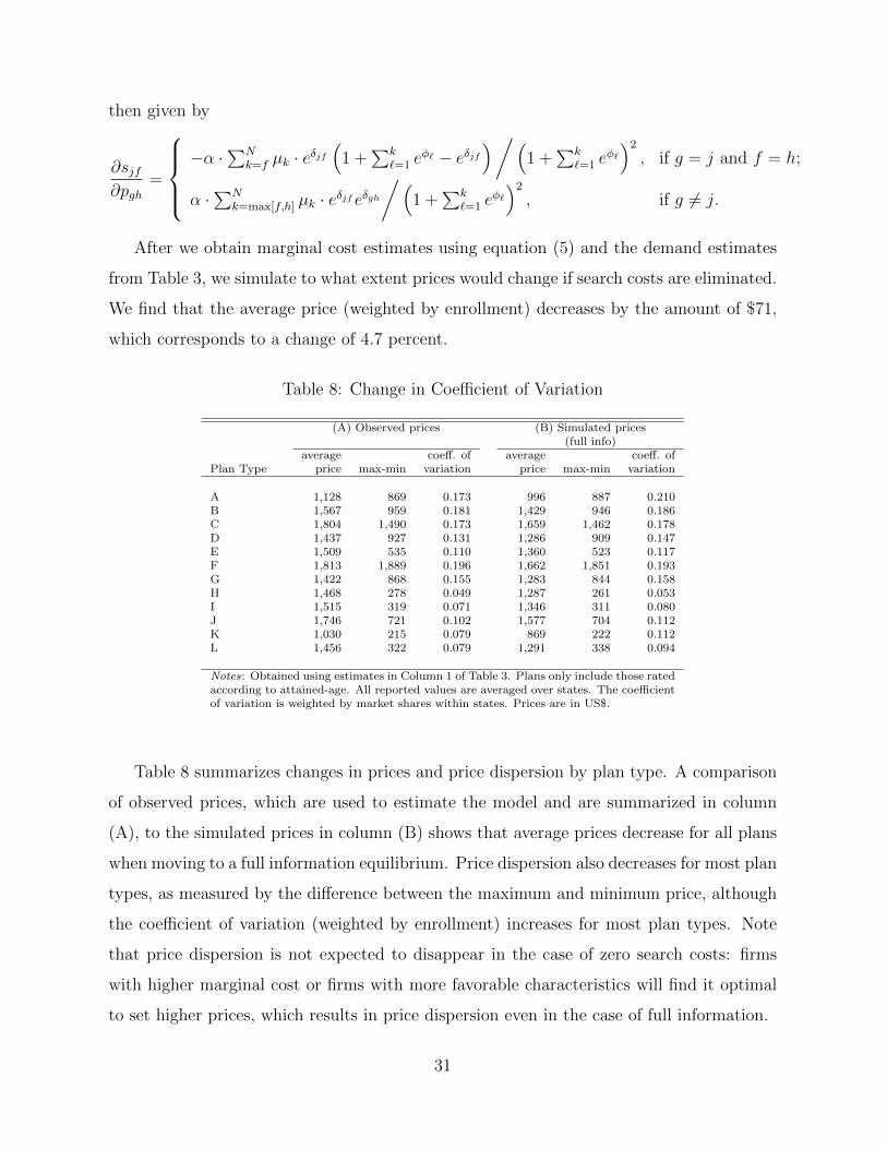
After we obtain marginal cost estimates using equation (5) and the demand estimates

from Table 3, we simulate to what extent prices would change if search costs are eliminated.

We find that the average price (weighted by enrollment) decreases by the amount of $71,

which corresponds to a change of 4.7 percent.

Table 8: Change in Coefficient of Variation

(A) Observed prices (B) Simulated prices(full info)

average coeff. of average coeff. ofPlan Type price max-min variation price max-min variation

A 1,128 869 0.173 996 887 0.210B 1,567 959 0.181 1,429 946 0.186C 1,804 1,490 0.173 1,659 1,462 0.178D 1,437 927 0.131 1,286 909 0.147E 1,509 535 0.110 1,360 523 0.117F 1,813 1,889 0.196 1,662 1,851 0.193G 1,422 868 0.155 1,283 844 0.158H 1,468 278 0.049 1,287 261 0.053I 1,515 319 0.071 1,346 311 0.080J 1,746 721 0.102 1,577 704 0.112K 1,030 215 0.079 869 222 0.112L 1,456 322 0.079 1,291 338 0.094

Notes: Obtained using estimates in Column 1 of Table 3. Plans only include those ratedaccording to attained-age. All reported values are averaged over states. The coefficientof variation is weighted by market shares within states. Prices are in US$.

Table 8 summarizes changes in prices and price dispersion by plan type. A comparison

of observed prices, which are used to estimate the model and are summarized in column

(A), to the simulated prices in column (B) shows that average prices decrease for all plans

when moving to a full information equilibrium. Price dispersion also decreases for most plan

types, as measured by the difference between the maximum and minimum price, although

the coefficient of variation (weighted by enrollment) increases for most plan types. Note

that price dispersion is not expected to disappear in the case of zero search costs: firms

with higher marginal cost or firms with more favorable characteristics will find it optimal

to set higher prices, which results in price dispersion even in the case of full information.

31

To analyze changes in consumer welfare when moving to full information, we use com-

pensating variation (see also Small and Rosen, 1981; Nevo, 2000), which in our search

model corresponds to

CV =

N∑k=1

µpostk

[ICpost − (k − 1)cpost

k

]−

N∑k=1

µprek [ICpre − (k − 1)cpre

k ]

α,

where IC = log

(1 +

k∑=1

eφ`)

is the logit inclusive value and ck is the average search cost

of consumers searching k times. This amounts to the expected maximum utility when

searching k times (measured in dollars by normalizing by the price coefficient), averaged

over all k groups of consumers, taking average search costs for individuals in each group

into account. For the case in which the new search costs are zero, we set µN = 1 while

all other µk’s are zero. The average change in consumer surplus (weighted by total state

enrollment) when moving to the simulated zero search cost equilibrium is $374, which is

more than five times the magnitude of the weighted average price decrease ($71). Such

changes in consumer welfare are driven by multiple factors such as savings on search costs,

reduction in premiums, and expansion of the total market.

Note that we assume the set of plans offered by each firm to be exogenous for tractability

of the model. An important extension for future research is to allow firms to optimally

decide on the plans they offer. It is also worthwhile to note that we do not specifically

model consumer selection into Medigap plans. The existing literature has found mixed

evidence of selection in Medigap plans (Fang et al., 2008). Due to regulations in Medigap

such as product standardization and guaranteed issue, we suspect that firms are limited in

their capability to engage in cream-skimming. Nevertheless, we do offer some discussion

on how our results would be affected if firms are able to take selection into account when

setting prices. One obvious complication is that marginal costs may be related to prices,

which leads to an additional channel through which prices affect profits. For example, an

increase in price may scare away price-sensitive consumers, who may be more likely to have

worse than average health conditions. In such a scenario marginal costs would be negatively

related to prices, which means our current model is likely to overestimate marginal costs

as well as the new equilibrium prices in the counterfactual in which we assume there are

no search frictions. Moreover, if this would be the case, our counterfactual results should

32

be considered as a lower bound on the predicted price decreases.

4 Monte Carlo Experiments

In this section we use several Monte Carlo experiments to study the performance of our

estimation procedure. Our first goal is to see whether our estimation procedure is able to

recover the search cost distribution as well as the parameters of the utility specification.

Next, we analyze the performance of our estimation procedure in situations where there

is heterogeneity in how consumers value observed characteristics. Our model is not able

to capture this, so we proceed by simulating data using a richer framework similar to

Moraga-Gonzalez et al. (2015), which allows us to assess to what extent search cost and

preference parameter estimates will be biased when using our model for estimation instead

of Moraga-Gonzalez et al.’s procedure.

The setup of the Monte Carlo experiments is as follows. We simulate data for 50 different

markets, where each market has three different firms, with each selling one product. Prices

are randomly drawn from a distribution that is uniform distribution between 3 and 4. We

allow for a constant as well as two product attributes that are randomly drawn from a

uniform distribution between 1 and 2, with parameter values as given by the first column

in Table 9. The unobserved characteristic is drawn from a normal distribution with mean

zero and standard deviation 0.1.

To see whether our estimation procedure is able to recover the parameters of the model

outlined in Section 2, we let consumers’ search costs be drawn from a lognormal distribution

with mean and standard deviation of the associated normal distribution set to zero and

three, respectively. Column (A) of Table 9 gives the mean and standard deviation of the

parameter estimates across 100 replications. All preference parameters are close to the

true coefficients and have low standard deviation. The reported search cost parameters are

obtained by fitting a lognormal distribution through the estimated points on the search

cost distribution and then averaged across the 100 replications. Both the mean and the

standard deviation parameters are close to the true coefficients. This is also shown in

Figure 3(a), which plots the estimated search cost CDF (solid curve), its 90% confidence

interval, and the actual CDF (black dashed curve).

33

Table 9: Results Monte Carlo Experiments

Main model Preference heterogeneityTrue (A) (B) σλ = 1.00 (C) σλ = 0.01

Variable Coeff. Coeff. Std.dev. Coeff. Std.dev. Coeff. Std.dev.

Preference parametersConstant -1.000 -1.086 (0.176) -2.109 (0.388) -2.063 (0.391)Attribute 1 4.000 4.011 (0.079) 3.368 (0.115) 4.127 (0.237)Attribute 2 2.000 2.012 (0.050) 1.651 (0.084) 1.992 (0.152)Price -3.000 -2.985 (0.050) -2.583 (0.104) -3.098 (0.182)

Search cost parametersMean 0.000 -0.026 (0.100) -6.449 (0.627) -4.209 (0.289)St.dev. 3.000 2.982 (0.110) 3.392 (0.499) 1.932 (0.256)

To get a better sense to what extent the estimates that are obtained using our procedure

are sensitive to preference heterogeneity in observed characteristics, Columns (B) and (C)

of Table 9 give results of Monte Carlo experiments in which we use a more general model

to generate the data, and use that data to estimate our model. The more general model

we use to generate the data is similar to the model in Moraga-Gonzalez et al. (2015). An

important difference between this model and our model is the way in which search costs

are modeled. Specifically, Moraga-Gonzalez et al. (2015) let search costs be consumer-

choice-set specific, i.e., consumer i’s search cost for choice set S is ciS = t′iSγ+σλλiS, where

t′iS contains a vector of search cost shifters, λiS is a consumer-choice-set specific search

cost error term with scale parameter σλ. According to Moraga-Gonzalez et al. (2015), by

assuming −λiS is IID Type I Extreme Value distributed, the probability that product j is

purchased is

sj =

∫sijdFτ (τi), (6)

where Fτ is the CDF of the vector of consumer-specific random variables τi and sij is the

probability that consumer i buys product j, i.e.,

sij =∑S∈Sj

emiS/σλ∑S′∈S e

miS′/σλ

eδij

1 +∑

r∈S eδir,

where miS = log(

1 +∑

j∈S eδij

)−t′iSγ and Sj is the set of choice sets that contains product

j.

We use the market share expression in equation (6) to generate data. We use the same

34

0.0 0.1 0.2 0.3 0.4 0.5 0.6c0.0

0.2

0.4

0.6

0.8

1.0CDF

(a) Search cost CDF main model

0.0 0.1 0.2 0.3 0.4 0.5 0.6c0.0

0.2

0.4

0.6

0.8

1.0CDF

(b) Search cost CDF preference heterogeneity

Figure 3: Search Cost Distribution Monte Carlo Experiments

preference parameters as we used to simulate the data for the main model, but in addition

we also allow for a random price coefficient. Specifically, we assume the distribution for the

price coefficient is normal with mean -3 and standard deviation 0.2. We assume one search

cost shifter, which, as in the main specification, is drawn from a log-normal distribution with

parameters zero and three. An important difference with our model is that consumers no

longer have a similar ranking of firms: because of the random price coefficient, a consumer’s

price sensitivity is going to affect her ordering of firms. Moreover, the choice-set specific

search cost shock creates additional randomness in consumers’ rankings of firms.

Moraga-Gonzalez et al. (2015) assume σλ = 1 when estimating their model, which is

also what we use to generate the data that is used in column (B) of Table 9. As shown

in the table, all the preference parameters as well as the mean search cost parameters are

more than two standard deviations away from the true coefficients. One reason for why

the estimates are very different is because of the relatively large variance of the choice-

set specific search cost error: the higher the scale parameter, the more likely it is that

lower ranked options are searched and the higher their market shares. To rationalize this

using our model, search cost estimates need to be lower than they really are. Column (C)

shows results when the data is generated using σλ = 0.01, which implies that the choice-

set specific search cost shock has a much smaller impact on the generated market shares,

making the model that is used to generate the data more similar to our model. Indeed,

all preference parameter estimates except for the constant are close to the true parameter

values. However, estimated search costs are still lower than the search costs that are used to

35

generate the model. This is also illustrated in Figure 3(b). The reason for this is that even

with a low variance of the search cost shock, lower ranked alternatives are still more likely

to be purchased than in our model, so if our model is used for estimation then relatively

low search costs are needed to explain the higher market shares for these products.

5 Conclusion and Discussion

In this paper we develop a model of consumer search to explain prices and price variation

for differentiated products. The model allows for both vertical and horizontal product

differentiation and can be estimated using constrained two-stage least squares. When

applying our model to the Medigap market, we find that our search model provides a better

fit than a model that assumes consumers have full information. Assuming full information

when consumers in fact have limited choice sets leads to a higher estimated price coefficient

in absolute sense. Search costs are large in this market: median search costs are estimated

to be $30. When moving to a zero-search-cost equilibrium, we find average prices fall by

$71 and average consumer welfare increases by $374.

One of our main contributions is to provide a methodology that allows us to non-

parametrically estimate search costs for differentiated goods when using only aggregate

data on consumer demand. Our model is general enough to be applied to markets in which

both search frictions and product differentiation coexist, and that lack suitable search cost

shifters. Monte Carlo simulations suggest estimation of utility parameters works reasonably

well even in situations where there is some heterogeneity in how consumer value observed

characteristics, although the results with respect to the estimated search costs should be

interpreted cautiously since search costs may be underestimated.

36

References

Anderson, S. and R. Renault (1999). Pricing, product diversity, and search costs: A

bertrand-chamberlin-diamond model. RAND Journal of Economics 30, 719–735.

Armstrong, M. (2017). Ordered consumer search. Journal of the European Economic

Association 15, 989–1024.

Berry, S., J. Levinsohn, and A. Pakes (1995). Automobile prices in market equilibrium.

Econometrica 63, 841–890.

Brown, J. R. and A. Goolsbee (2002). Does the internet make markets more competitive?

evidence from the life insurance industry. Journal of Political Economy 110, 481–507.

Burdett, K. and K. L. Judd (1983). Equilibrium price dispersion. Econometrica 51, 955–

969.

Carlson, J. A. and R. P. McAfee (1983). Discrete equilibrium price dispersion. Journal of

Political Economy 91, 480–493.

Cebul, R. D., J. B. Rebitzer, L. J. Taylor, and M. E. Votruba (2011). Unhealthy insur-

ance markets: Search frictions and the cost and quality of health insurance. American

Economic Review 101, 1842–1871.

Chade, H. and L. Smith (2006). Simultaneous search. Econometrica 74, 1294–1307.

Fang, H., M. P. Keane, and D. Silverman (2008). Sources of advantageous selection: Evi-

dence from the medigap insurance market. Journal of Political Economy 116, 303–350.

Hausman, J. A. (1996). Valuation of new goods under perfect and imperfect competition.

In T. F. Bresnahan and R. J. Gordon (Eds.), The Economics of New Goods, Volume 58.

National Bureau of Economic Research.

Honka, E., A. Hortacsu, and M. A. Vitorino (2017). Advertising, consumer awareness,

and choice: evidence from the U.S. banking industry. RAND Journal of Economics 48,

611–646.

37

Hortacsu, A. and C. Syverson (2004). Product differentiation, search costs, and competition

in the mutual fund industry: a case study of S&P 500 index funds. Quarterly Journal

of Economics 119, 403–456.

Ly, D. P., S. Sheingold, and A. Shartzer (2011). Variation and trends in medigap premiums.

Aspe report, U.S. Department of Health and Human Services.

Maestas, N., M. Schroeder, and D. Goldman (2009). Price variation in markets with

homogeneous goods: The case of medigap. NBER Working Paper No. 14679.

Moraga-Gonzalez, J. L., Z. Sandor, and M. R. Wildenbeest (2015). Consumer search and

prices in the automobile market. Working paper, Indiana University.

Nevo, A. (2000). Mergers with differentiated products: the case of the ready-to-eat cereal

industry. RAND Journal of Economics 31, 395–421.

Robst, J. (2006). Estimation of a hedonic pricing model for medigap insurance. Health

Services Research 41, 2097–2113.

Small, K. A. and H. S. Rosen (1981). Applied welfare economics with discrete choice

models. Econometrica 49, 105–130.

Sorensen, A. T. (2000). Equilibrium price dispersion in retail markets for prescription

drugs. Journal of Political Economy 108, 833–850.

Stahl, D. O. (1989). Oligopolistic pricing with sequential consumer search. American

Economic Review 79, 700–712.

Starc, A. (2014). Insurer pricing and consumer welfare: Evidence from medigap. RAND

Journal of Economics 45, 198–220.

Stigler, G. (1961). The economics of information. Journal of Political Economy 69, 213–

225.

Weitzman, M. L. (1979). Optimal search for the best alternative. Econometrica 47, 641–

654.

38

Wildenbeest, M. R. (2011). An empirical model of search with vertically differentiated

products. RAND Journal of Economics 42, 729–757.

Wolinsky, A. (1986). True monopolistic competition as a result of imperfect information.

Quarterly Journal of Economics 101, 493–511.

39