Search and Information Frictions on Global E-Commerce

Platforms: Evidence from AliExpress∗

Jie Bai Maggie X. Chen

Harvard Kennedy School George Washington University

& NBER

Jin Liu Xiaosheng Mu Daniel Yi Xu

New York University Princeton University Duke University

& NBER

September 14, 2021

Abstract

We study how search and information frictions shape market dynamics in globale-commerce. Observational data and self-collected quality measures from AliExpressestablish the existence of search and information frictions. A randomized experimentthat offers new exporters exogenous demand and information shocks demonstratesthe potential role of sales accumulation in enhancing seller visibility and overcomingthese demand frictions. However, we show theoretically and quantitatively that thisdemand-reinforcement mechanism is undermined by the large number of online ex-porters. Our structural model rationalizes the experimental findings and quantifiesefficiency gains from reducing the number of inactive sellers.

Keywords: global e-commerce, exporter dynamics, product quality, information frictions, search

frictions

JEL classification: F14, L11, O12

∗We thank Costas Akolakis, Treb Allen, David Atkin, Oriana Bandiera, Abhijit Banerjee, Heski Bar-Isaac,Lauren Bergquist, Davin Chor, Dave Donaldson, Esther Duflo, Ben Faber, Gordon Hanson, Chang-tai Hsieh,Panle Jia, Amit Khandelwal, Asim Khwaja, Pete Klenow, Danielle Li, Rocco Macchiavello, Isabela Manelici,Nicholas Ryan, Meredith Startz, Tianshu Sun, Christopher Snyder, Catherine Thomas, Eric Verhoogen, DavidWeinstein, and seminar and conference participants at Berkeley Economics, BREAD/CEPR/STICERD/TCDConference, University of Chicago, Harvard Kennedy School, Hong Kong Trade Workshop, IPA SME WorkingGroup Meeting, Michigan Economics, NBER Conferences (China Working Group, DEV, ITI, IT/Digitization),USC, Fudan, and IADB for helpful comments. We thank Zixu Chen, Chengdai Huang, Haoran Zhang, and QiangZheng for excellent research assistance. All errors are our own.

1 Introduction

E-commerce sales have grown tremendously in recent years, reaching $2.9 trillion in 2018 and

12% of total global retail sales (Lipsman, 2019). Within e-commerce, cross-border sales have

grown twice as fast as domestic sales, and nearly 40% of online buyers completed a cross-border

transaction in 2016 (Pitney Bowes, Inc, 2016). By extending market access beyond geographical

boundaries, global e-commerce platforms present a promising avenue for small and medium-

sized enterprises (SMEs) in developing countries to enter export markets. Furthermore, online

exporting lowers many of the traditional barriers of exporting, including the need to build export

relationships and set up distributional channels in destination countries.1 Given these promises

and the large market potential, numerous policy initiatives have been adopted worldwide to foster

e-commerce growth (e.g, UNCTAD, 2016), with a specific policy target to onboard developing-

country SMEs onto e-commerce platforms and allow them to tap into the global market.

Despite the rapid growth of global e-commerce, there is a lack of empirical evidence on

the impact of the increased export opportunities on firm growth and market dynamics. While

e-commerce potentially exposes prospective exporters to buyers around the world, the sheer

number of firms operating on these platforms can create substantial congestion in consumer

search.2 When firms’ intrinsic quality is not perfectly observed, search frictions can further slow

down resolution of the information problem and hinder market allocation toward better firms.

In this study, we experimentally, theoretically, and quantitatively investigate how these

demand-side frictions shape market dynamics in global e-commerce. We first document de-

scriptive evidence consistent with sizable search and information frictions in global online mar-

ketplaces. Next, we experimentally identify and demonstrate the role of demand accumulation

in helping firms overcome these frictions by improving firms’ visibility and generating future de-

mand. Motivated by the reduced-form evidence, we develop a theoretical model that formalizes

this demand-driven reinforcement channel under search and information frictions and character-

ize its efficiency implications. Building on the theoretical framework, we estimate a rich empirical

model of the online export market and use the model estimates to quantify the impacts of search

and information frictions on firm growth, market allocation, and consumer welfare. Finally, we

apply our model to shed light on policies that could facilitate the growth of promising export

1For example, AliExpress, a leading cross-border e-commerce platform that we study in this project, stateson its website (https://sell.aliexpress.com/), “Set up your e-commerce store in a flash, it’s easy and free!Millions of shoppers are waiting to visit your store!”

2The logic of this effect can be traced to Stigler (1961), in which consumers are not perfectly informed aboutall products available for purchase in a given market and can only consider a limited subset.

1

businesses beyond the initial onboarding stage and improve overall market efficiency.

Our study is grounded in the context of AliExpress, a world-leading B2C cross-border e-

commerce platform owned by Alibaba. We focus on the industry of children’s T-shirts and

collect comprehensive data about sellers operating in this industry, including detailed seller-

product-level characteristics and transaction-level sales records. We complement the platform

data with a novel set of objective, multidimensional measures of quality, ranging from detailed

product quality metrics to shipping and service quality indicators. These measures are collected

by the research team based on actual online purchases and direct interactions with the sellers as

well as third-party assessments.

We begin by documenting a set of new stylized facts about the online exporters. First, we

compare the sales distribution within identical-looking product varieties. Interestingly, even after

we control for horizontal taste differences, there remains meaningful dispersion in sales within

identical-looking variety groups, as opposed to “winner-takes-all.” This finding is indicative of

search frictions: buyers, upon arriving on the platform, face thousands of product offerings but

can consider only a finite subset of all seller listings.3 This raises the question of who gets to grow

in the presence of these search frictions. Next, we dive further into the potential determinants

of growth and find that quality only weakly predicts sales. The “superstars,” which we define

as the largest seller in each product variety, do not necessarily have the highest quality (or the

lowest price). Intuitively, search frictions introduce a random component in firm growth due to

the consumer sampling process. When firms’ intrinsic qualities are not perfectly observed (even

after they enter a consumer’s search set), such frictions can further slow down the revelation

of true quality, leading to potential market misallocation. Finally, we find robust evidence that

current sales predict the speed of arrival for future sales. This implies that firms with larger past

sales—and hence higher visibility—have an advantage in overcoming consumer search frictions

and generating future orders. However, if information frictions prevent a firm’s visibility from

being aligned with its fundamentals, it could take much longer for better firms to distinguish

themselves. Overall, market allocation and consumer welfare depend crucially on the interactions

of these demand-side forces.

Our interpretation of the stylized facts highlights a demand-reinforcement mechanism where

accumulating sales boosts a firm’s visibility and helps attracting future sales. Having said that,

unobserved supply-side actions (such as advertising and display) could also exist and lead to

3This is consistent with prior studies that find substantial price dispersion in online marketplaces even foridentical products, indicating the presence of significant search frictions (e.g., Clay et al., 2001; Clemons et al.,2002; Hortacsu and Syverson, 2004; Hong and Shum, 2006).

2

similar reduced-form relationships between current sales and future sales. To further establish

the empirical validity of the demand mechanism, we conduct an experiment in which we generate

exogenous demand shocks to a set of small exporters via randomly placed online purchase or-

ders. Since how effectively the additional demand conveys the firm’s true fundamentals depends

critically on the severity of information frictions, we further interact the order treatment with a

review treatment about firms’ product and shipping quality to examine the role of information

provision. We find that the order treatment leads to a small but significantly positive impact on

firms’ subsequent sales, establishing the demand mechanism. We document supporting evidence

that this effect is mediated by a short-term boost in a listing’s ranking and is unlikely to be driven

by endogenous supply-side responses. In the meantime, we do not find any significant treatment

effect from the reviews, suggesting that the online reputation mechanism may not function very

effectively in the presence of large search frictions. This outcome echoes the stylized fact that

quality does not strongly predict growth in this market due to the search and information prob-

lems, which, when combined together, make it particularly difficult for high-quality sellers to

stand out. Using cumulative sales measured at the endline, we estimate an average treatment

effect that is much smaller than the size of the initial treatment (0.1-0.25 versus 1), suggesting

that the frictions cannot be easily overcome by an individual seller’s private effort.

All together, the descriptive and experimental findings are consistent with the presence of

sizable search and information frictions and establish an important demand-reinforcement mech-

anism of online firm growth. Motivated by the reduced-form evidence, we develop a theoretical

model that formalizes the process of demand accumulation under consumer search and learning

and use the model to examine the efficiency properties of the market. The model extends the

classical Polya urn model by incorporating consumer choice and seller heterogeneity in quality.

In every period, consumers conduct a fixed sample search where the probability of a seller being

sampled is proportional to a power function of its cumulative sales. Consumers observe noisy

signals of seller quality based on past reviews and make purchase decisions based on expected

quality within the search sample. To examine the implications of search and information fric-

tions, we focus our theoretical analysis on a key comparative static with respect to the number

of sellers: while e-commerce lowers the entry barriers to exporting and brings many firms on-

line, the presence of a large number of sellers can exacerbate congestion in consumer search and

slow down the rise of high-quality sellers, given consumers’ limited search sample size. Tying this

analysis back to our policy motivation, we prove theoretically that indeed when there are already

many sellers in the market, further increasing the number of sellers strictly worsens allocation

3

and welfare along the path of market evolution.

Building on the theoretical framework, we estimate a rich empirical model of the online mar-

ket. We follow the setup of the theoretical model closely and extend the setup to incorporate

seller-side heterogeneity in both quality and cost and model sellers’ pricing decisions. Our esti-

mate implies that compared with sellers who have made zero sales, sellers who strike a first order

are 4.6 times more likely to end up in a subsequent consumer’s search sample. Nonetheless, due

to the information problem, uncertainty regarding the seller’s quality still remains even after the

seller successfully strikes the first sale. Our estimate of the review signal noise implies that the

posterior uncertainty is reduced by only 3.3% after the first order. This suggests that online

reviews are very noisy signals about sellers’ quality and that the informational uncertainty is re-

solved very slowly, i.e., only after a seller accumulates a substantial number of orders. Combined,

these findings highlight that search frictions, interacted with information frictions, can constitute

an important hurdle for the growth of small prospective exporters. Using the experiment as a

model validation benchmark, we find quantitatively comparable average treatment effects when

we simulate one-time demand shocks through the lens of the model.

We end with several counterfactual exercises to examine the distinctive roles of search and

information frictions in firm growth and market allocation and use the estimated model to evalu-

ate potential policy interventions. First, we investigate the impact of lowering search frictions by

reducing the number of sellers operating on the platform. The results show that doing so helps

mitigate congestion in consumer search, thereby improving allocative efficiency and consumer

welfare (as in our theoretical analysis). The improvement is especially strong when there exist

large information frictions. This result serves as a cautionary tale against blanket onboarding

initiatives that try to bring many firms online: simply giving firms easy access to foreign markets

may not be sufficient for generating sustained growth and can in fact exacerbate search and

information problems, resulting in market misallocation.

Next, to shed light on the role of information frictions, we remove the noise from the review

signals. We find that doing so significantly shifts market share to high-quality sellers and raises

consumer surplus. We further decompose this welfare gain into a static gain (better decision-

making conditioning on a search sample) and a dynamic gain (better sample quality over time)

and find that the latter plays an important role. This result further highlights the important

interaction between search and information frictions.

Last but not least, we evaluate a potential policy, common among existing successful plat-

forms, to reduce search congestion by establishing a premium market segment that eliminates

4

a large number of inactive product listings and sellers. The key question for emerging new e-

commerce export platforms in developing economies is when to introduce such segmentation.

The key tradeoffs are again highlighted by our theoretical channels based on search and infor-

mation frictions: on the one hand, segmenting the market in the early stage, such as during the

initial onboarding stage when the market is just created, effectively reduces search congestion

and facilitates faster allocation of market share toward higher-quality sellers. On the other hand,

segmenting the market too early results in loss of information that could be revealed through

sellers’ performance over time. We show that welfare is indeed nonmonotonic with respect to

the timing of implementation, reflecting the balance between the underlying economic forces.

While our setting is specific to e-commerce, the economic insights generalize to broader market

settings. It is well understood that there may be excessive entry when firms do not internalize

their “business-stealing” from competitors (Mankiw and Whinston, 1986). Our paper illustrates

that with the presence of search frictions, such business-stealing can happen when sellers compete

for customer attention, beyond simple price competition. We further show that the business-

stealing effect can be particularly costly when there exist information frictions, which prevent

the best firms from being discovered and reduce the allocative efficiency of the market. Several

features of the cross-border e-commerce setting make it a good exhibit of these economic forces:

specifically, the lack of market selection, which results in excessive entry, and differences in

cultural and business practices across borders, which aggravate the information problem.

Related Literature. Our work contributes to several strands of the existing literature. A large

literature in trade and development has documented the important role of quality in determining

exporter performance (see Verhoogen, 2020 for an excellent review). We build on a growing body

of research that collects detailed information on quality for specific industries (e.g., Atkin et al.,

2017; Macchiavello and Miquel-Florensa, 2019; Bai et al., 2019; Hansman et al., 2020). Similar

to these earlier works focused on offline settings, we document large variations in firm-product

quality in the online marketplace. However, we find that quality plays a less pronounced role in

explaining exporter growth and long-run market shares. Our paper highlights the role of search

and information frictions in explaining the disintegration of the customer accumulation process

and firms’ fundamental quality. Leveraging unique quality data, we further quantify the scope

of market misallocation through the lens of a rich empirical model.

Relatedly, our paper also speaks to the existing literature in trade and development on search

and information frictions (Allen, 2014; Macchiavello and Morjaria, 2015; Steinwender, 2018;

Startz, 2018). Theoretically, we formalize the process of consumer search and learning and derive

5

the efficiency implications for short- and long-run market outcomes, highlighting the important

interplay between the demand-side frictions and the number of market participants. Empirically,

we bring in new sources of variations to first experimentally identify a demand-reinforcement

mechanism that can potentially help firms overcome these frictions. We then formally model

these realistic market frictions and quantify their impacts on market dynamics and consumer

welfare. Methodologically, our paper is closely related to Atkin et al. (2017), which also studies

the impact of foreign demand shocks on exporters, showing that firms respond to these demand

shocks by improving quality through learning by doing. Rather than focusing on firms’ own

actions, we explore how foreign demand shocks improve firm visibility and help them overcome

market search and information frictions.

Third, our work relates to the extensive literature on new exporter dynamics, primarily in

the offline setting. A common empirical pattern that emerges from micro data is that young

exporting firms start small and have high turnover rates, and those that survive experience rapid

growth. Various theoretical mechanisms have been proposed to explain these facts. They include

firm learning (Arkolakis et al., 2018; Ruhl and Willis, 2017), demand accumulation (Foster et al.,

2016; Piveteau, forthcoming; Fitzgerald et al., 2020), and seller search (Eaton et al., 2016). In

contrast to these studies, our paper focuses on demand-side frictions as the key driving force of

firm and market dynamics in the online setting. In particular, unlike in the offline export market,

the fixed costs of operating are substantially lower in online marketplaces, significantly weakening

the role of market selection. Our work shows how the lack of selection reduces consumer search

efficiency and endogenously slows down the growth of high-quality exporters.

Lastly, our study also relates to the existing literature on consumer search and consumer

consideration sets (for example, Goeree, 2008; Kim et al., 2017; Honka et al., 2017; Dinerstein et

al., 2018).4 We extend existing search models, which have assumed that consumers can perfectly

learn a product’s utility after a single search, by incorporating information frictions and a process

of consumer learning enabled by the online review mechanism (Tadelis, 2016). This approach

allows us to examine the interaction between search and information frictions.5

The remainder of the paper is organized as follows. Section 2 describes the empirical setting

and data. Section 3 presents a set of stylized facts about online exporters and motivates the

4We refer interested readers to a recent article by Honka et al. (2019) for a review of the broader literature.5In a different setting, Pallais (2014) and Stanton and Thomas (2016) examine information frictions in online

labor markets and show that information generated from initial hires affects workers’ subsequent hiring outcomes.In a similar vein, we show that initial demand generated from past purchases affects subsequent growth of firms.We further introduce search frictions and show that doing so exacerbates the initial hurdle for high-quality newbusinesses to distinguish themselves.

6

experiment. Section 4 describes the experiment design and main findings. Section 5 develops

the theoretical model and derives market efficiency properties. Section 6 builds and estimates

an empirical model of the online market. Section 7 performs counterfactual analyses. Section 8

concludes.

2 Empirical Setting and Data

In this section, we introduce the study setting, the market for children’s T-shirts on AliExpress,

and describe the data collection.

2.1 The Market for Children’s T-shirts on AliExpress

AliExpress, a subsidiary of Alibaba, was founded in April 2010 to specialize in international

trade. As a global leading platform for cross-border B2C trade, AliExpress serves over 150

million consumers from 190 countries and regions, attracting over 200 million monthly visits.6

Over 100 million products, ranging from clothes and shoes to electronics and home appliances,

and 1.1 million active sellers, primarily retailers located in China, are listed on the platform.7

Most sellers on the platform are retailers, rather than manufacturers, and source products from

factories all over the country to export through the platform. Therefore, quality, in this context,

captures firms’ sourcing ability (i.e., ability to source high-quality products from manufacturers)

as well as the quality of their marketing and shipping services.8

For this study, we focus on the children’s T-shirt industry. As the largest textile and garment

exporting country in the world, China accounted for over a third of the world’s total textile

and garment exports in 2019 (WTO, 2020). In the world of e-commerce, textile and apparel

amount to 20 percent of China’s total online retail, including sales on Alibaba’s platforms.9 The

growth and efficiency of the online retail market therefore matters for upstream manufacturing:

in particular, growth of retailers that sell high-quality products in turn benefits their producers.

6Sources: https://sell.aliexpress.com/.7During our sample period, AliExpress hosted sellers from mainland China only; starting in 2018, the platform

also became available to sellers in Russia, Spain, Italy, Turkey, and France.8While most of the sellers on the e-commerce platform are retailers instead of manufacturers, quality may

still vary significantly depending on where the sellers choose to source from—whether high-quality or low-qualityfactories—and how much quality inspection effort they put in. We document this formally using detailed qualitymeasures that we collect from the study in Section 2.2.

9“E-Commerce of Textile and Apparel,” China Commercial Circulation Association of Textile and Apparel,2019.

7

The vibrant entry and growth dynamics in the online market also provide an ideal setting for

studying exporter dynamics. In addition, the T-shirt product category features well-specified

quality dimensions, making it possible to construct direct quality measures to study quality-size

distributions and allocative efficiency.

Two features of the platform are worth highlighting. First, AliExpress does not require a

sign-up fee to set up a store and list a product, thereby essentially eliminating entry and fixed

operation costs of exporting and allowing sellers large and small to tap into export markets.10

While this helps bring many SMEs onto the platform, the lack of market selection can create

important congestion in consumer search, resulting in an excessive number of firms and product

offerings competing for consumers’ attention in the online marketplace. The resulting welfare

implications of the increasing number of market participants for firms and consumers are far less

clear in the presence of search and information frictions. The nature of this tradeoff is the key

question that we seek to examine in this study.

Second, AliExpress allows us to group product listings into different varieties. A single variety

group (hereafter referred to as a group) may contain multiple listings that are sold by different

sellers but share an identical product design. This is illustrated in Figure 1. This unique feature

allows us to compare listings with the same observable product attributes, thereby controlling

for consumers’ horizontal taste differences. We leverage this feature in our empirical analysis as

described below.

2.2 Data

We collect comprehensive data from the platform, including detailed firm-product-level charac-

teristics and transaction-level sales records. We complement the platform data with objective

quality measures obtained from actual purchases, direct interactions with sellers, and third-party

assessment. Below, we describe the sample and the key variables used in the analyses.

(1) Store-Listing-Level Data. We scraped nearly the full universe of product listings in the

children’s T-shirt industry in May 2018.11 We collected all the information that a buyer can view

on the listings’ pages, including total cumulative orders (quantity sold), current prices, discounts

(if any), ratings, buyer protection schemes (if any), and detailed product attributes. We further

10AliExpress charges sellers 5-8% of their sales revenue as a commission fee for each successful transaction.Source: https://sell.aliexpress.com/.

11The scraping was done at the group level. The platform allowed users to view the first 99 pages of varietygroups with 48 groups per search page.

8

collected information about the stores that carry these products, including the year of opening

and other products that the stores carry.

Table 1 summarizes the product-listing-level (Panel A) and store-level (Panel B) character-

istics. There are 10,089 product listings in total. The average price is $6.1. Approximately

54% of the listings offer free shipping, and the average price of shipping to the US is $0.63. At

the store level, there are 1,291 stores carrying these products. Most exporters are young, with

an average age of 1.61 years. The average cumulative sales is 235 with a standard deviation

of 970, indicating large performance heterogeneity. We observe similar patterns of performance

heterogeneity at the listing level. At a given point in time, more than 35% of the listings have

zero sales, and the median has 2, whereas the largest listing has 10,517 orders accumulated.

(2) Transaction Records. We take advantage of a unique feature of AliExpress during our

sample period that allows us to keep track of a listing’s most recent six-month transaction history.

For each transaction, we observe information on sales quantities, ratings, and previous buyers’

countries of origin. In contrast, most existing e-commerce platforms (e.g., Amazon and eBay)

report only customer reviews and the total volume of transactions, not the full transaction

history. The availability of the real-time transaction records enables us to closely track each

product listing’s sales activities over time.

(3) Measures of Quality. Finally, we complement the platform data with a rich set of objective

quality measures collected through (i) actual purchases of the products, (ii) direct communica-

tions with the sellers, and (iii) third-party assessment. To collect the quality data, we focus on

variety groups with at least 100 cumulative sales (aggregated across all listings in the group) to

focus on products that are more relevant for consumer choice. This leaves us with 1,258 product

listings sold by 636 stores in 133 variety groups, with varying performance heterogeneity (mea-

sured in terms of cumulative sales) within each group. All together, the measures cover multiple

dimensions of quality, ranging from product to service to shipping quality.

To measure product quality, we placed actual orders for children’s T-shirts on AliExpress.12

After receiving and cataloging the orders, we worked with a large local consignment store of

12Measuring product and shipping quality involves actually purchasing the T-shirts. Therefore, we combinedthis data collection effort with the experiment in which we generated exogenous demand shocks to a randomlyselected subset of treated small listings (with fewer than 5 cumulative orders) in the 133 variety groups. Hence,the sample for product quality consists of all treated small listings (with fewer than 5 cumulative orders) in theexperiment described in Section 4 and their medium-size (with cumulative orders between 6 and 50) and superstar(with the largest number of cumulative orders) peers in the same variety groups. This sampling procedure aimedto achieve two goals: first, it allowed us to obtain product and shipping quality measures for listings with differentbaseline sales to examine quality-sales relationships; second, it ensured that we have a control group of identicalsmall listings not receiving any purchase order treatment.

9

children’s clothing in North Carolina to inspect and grade the quality of each T-shirt. The grading

was done on a rich set of metrics, following standard grading criteria used in the textile and

garment industry. Specifically, product quality was assessed along eight dimensions: durability,

fabric softness, wrinkle test, seams (straightness and neatness), outside stray threads, inside

loose stitches, pattern smoothness, and trendiness. Figure A.1 Panel A shows a picture of the

grading process and the criteria used. Quality along each dimension was scored on a 1-to-5 scale,

with higher numbers denoting higher quality. Most of the quality metrics (with the exception of

trendiness) capture vertical quality differentiation. For example, at equal prices, consumers prefer

T-shirts with more durable fabric, straighter seams and fewer stray loose threads. Exploiting

the grouping function, we can further compare quality across T-shirts of the exact same design

but sold by different sellers. As shown in Panel B of Figure A.1, there exist considerable quality

differences both across and within variety groups, depending on which factories the retailers

choose to source from and/or how much quality inspection effort they put in.

To measure shipping quality, we recorded the date of each purchase, date of shipment, date

of delivery, carrier name, and condition of the package upon arrival. The information is used

to construct three measures of shipping quality: (i) the time lag between order placement and

shipping, (ii) the time lag between shipping and delivery, and (iii) whether the package was

damaged.

To measure service quality, we visited the homepage of each store and sent a message to the

seller via the platform to inquire about a particular product.13 We rate service quality based on

the time it took to receive a reply, in particular, whether the message was replied to within two

days (which represents the 70th percentile in reply time). Appendix B.1 provides more details

of the quality measurement process.

Panels A and B in Table 2 present summary statistics of the various quality measures. For the

empirical analysis, we construct different quality indices by first standardizing the detailed quality

measures in each dimension and then averaging them within and across the three dimensions.

Panel C in Table 2 summarizes the distribution of the quality indices. Table A.1 decomposes the

variation of the overall quality index into that explained by each individual quality metric.

To cross-validate these objective quality measures, we first examine the relationships between

them and the online ratings and find all three quality indices—product, shipping and service—to

be positively correlated with the online star ratings and—in the case of shipping and service

13To measure service quality, we reached out to all 636 stores in the 133 variety groups. For those with multiplelistings included in the 133 groups, we randomly selected one listing to inquire and assign the same service qualityscore to all listings sold by the same seller.

10

quality—statistically significant, as shown in Table A.2. For product quality, we further asked

the owner of the consignment store to report a bid price (willingness to pay) and a resell price

for each T-shirt. Reassuringly, the objective product quality metrics are strongly correlated with

the price evaluations. Last but not least, to corroborate the measures of service quality, we sent

multiple rounds of messages to the same stores and tracked sellers’ replies. Table A.3 shows that

a seller’s reply speed is highly consistent over time.14

3 New Stylized Facts about Online Exporters

Using the newly assembled micro dataset, we begin by documenting a set of new stylized facts

about online exporters. These facts provide suggestive evidence of the presence of search and

information frictions and, at the same time, highlight a demand-reinforcement mechanism that

can potentially help sellers overcome these frictions and grow.

Fact 1. Sales performance varies within identical-looking variety groups.

First, we exploit the grouping feature described in Section 2.1 that allowed us to group

product listings into different identical-looking varieties to examine how sales performance varies

within a single variety group. As shown in Figure 2, we see that sales are concentrated at the

top within each group. The group’s superstar, defined as the listing with the highest number of

cumulative orders within the group, accounts for about 63.8% of the total sales of the group; the

top 25% capture nearly all sales (90.3%).

Nonetheless, the distribution of superstar sales across groups makes clear that this is not a

case of a winner-take-all market; some amount of dispersion still remains. Given that we are

comparing products with essentially identical designs, we are controlling for unobserved consumer

horizontal tastes. In a frictionless world, we may expect that the listing with the highest quality,

relative to price, would win the market.15 The fact that some dispersion remains indicates that

14We appreciate this suggestion made by various seminar and conference participants, which led us to revisitthe platform in June 2021 and collect 3 rounds of service quality data following the exact same procedure for anew sample of 132 stores with active listings in children’s T-shirts (in popular variety groups) at the time. Poolingdata across all the 132 stores over 3 rounds, we estimate intracluster correlations as high as 0.5, 0.51, and 0.48for the 3 quality measures examined in Table A.3, respectively. Regressing the reply behavior measured in thesecond and third rounds (stacked) on that in the first round yields positive coefficients of 0.614, 0.562, and 0.591,which are highly significant at the 1% level, as shown in Table A.3.

15Part of the dispersion could be due to heterogeneous preferences for quality and price among consumers.To examine this possibility, we leverage the six-month transaction data, in which we observe buyers’ country oforigin, to examine sales performance within identical-looking variety groups by country (where we restrict salesto a given country and define the top sellers for each country separately). Figure A.2 shows the patterns for the

11

frictions exist in this marketplace. This raises the question of who gets to grow in the presence

of these frictions. To delve deeper into this issue, we next ask who gets to become superstars.

Fact 2. Superstars do not necessarily have the highest quality, and quality only weakly predicts

sales.

We compare the quality of the superstar listings and small listings in each variety group using

the objective quality measures described in Section 2.2. A superstar is defined as the listing with

the highest sales in the group, and small listings are those with fewer than 5 cumulative orders.

Panel A of Figure 3 plots the distribution of the difference in the overall quality index between

the group superstar and the average of the small listings in each group. We observe a substantial

fraction below zero: superstars actually have lower quality than the small listings in 45% of the

variety groups sampled. In line with this, Panel B looks at how quality predicts sales. We see

that the average market share of a listing only weakly increases with quality. The difference is

not significant except at the top.

These observations indicate the difficulties that high-quality sellers face in gaining market

share due to search and information frictions. Intuitively, search frictions introduce a random

component in firm growth due to the consumer sampling process. When firms’ intrinsic qualities

are not perfectly observed, such frictions can further slow down resolution of the information

problem and hinder market allocation toward better firms. That said, this evidence is only

suggestive because we have to take into account price differences.16 To isolate the role of search

and information frictions and quantify the degree of misallocation, we rely on a structural model

in Section 6.

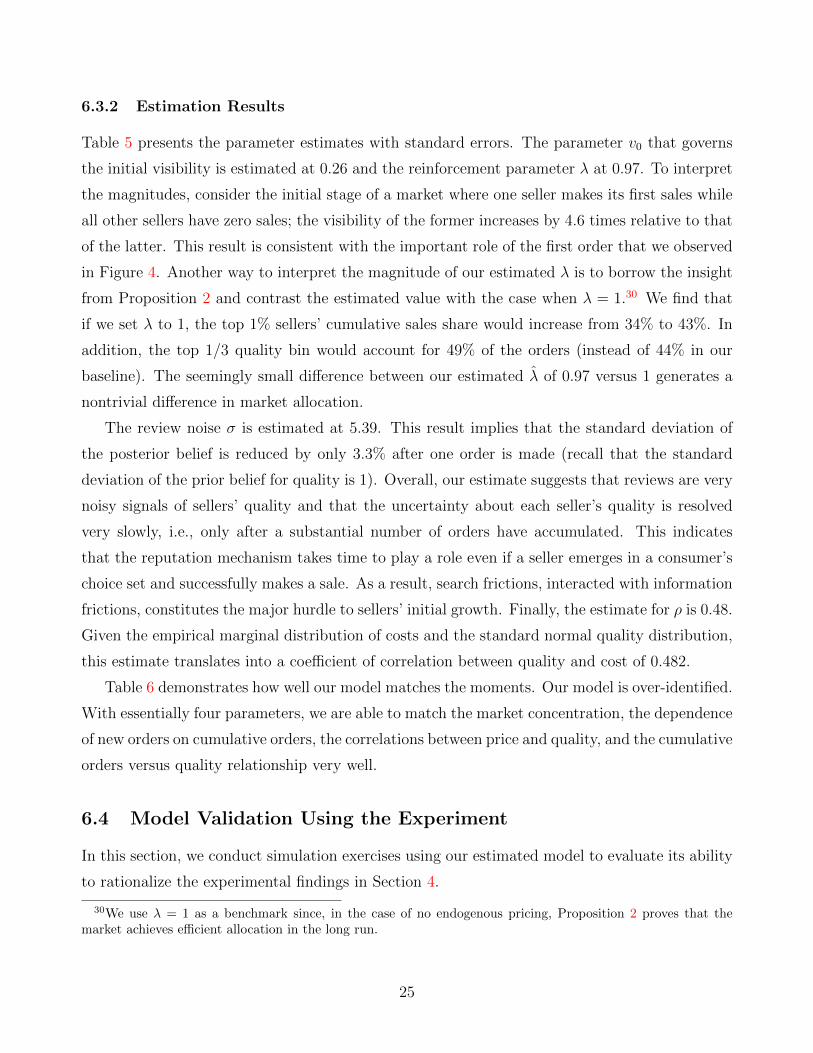
Fact 3. On average, it takes 79 days for the first order to arrive; after this period, subsequent

orders arrive much faster.

Finally, we delve further into the growth dynamics and examine how superstars emerge. Using

the transaction-level data from the six-month period from March to August 2018, we explore the

dynamics of order arrivals. Figure 4 plots the number of days that it takes to receive the n-th

order. Panel A shows the order arrival dynamics for the full unbalanced sample of all listings;

US and Russia. To the extent that consumers’ tastes are more similar within a country than across countries,the fact that we still observe a sizable amount of dispersion at the top suggests that not all of it is explained byheterogeneous preferences.

16Interestingly, we find that superstars do not always charge the lowest price, either: within an identical-lookingvariety group, the listing with the highest sales charges the lowest price only 14% of the time. On the other hand,we do observe a positive relationship between price and quality, which corroborates our quality measures butcould mean that this relatively flat relationship between quality and sales may be partly driven by price.

12

Panel B is restricted to listings that accumulated more than 10 orders during the six-month

period. A striking pattern emerges: on average, it takes 70-79 days for the first order to arrive;

however, conditional on receipt of one order, subsequent orders arrive much faster. For example,

on average, the second order arrives 7-15 days after the first order, and the third order arrives

4-6 days after the second. Table A.4 regresses the dummy of receiving an order in a given week

on the logged past cumulative orders of a product listing, with and without store fixed effects.

The results highlight a potential demand-reinforcement mechanism: that is, sellers with larger

past sales—and hence higher visibility—have an advantage in overcoming search and information

frictions and generating future sales.

However, a key empirical challenge in identifying the role of this demand-side effect is to

control for unobserved supply-side actions. For example, it could be that after some initial

period of preparation, sellers start to invest in some costly actions, such as paying for advertising

or participating in sales and promotion events organized by the platform, which then lead to the

first order and subsequent orders. From the observational data, it is difficult to tease apart the

demand- and supply-side channels. This motivates us to conduct an experiment to identify the

role of demand.

4 Experiment and Findings

To demonstrate the role of demand in helping firms overcome search and information frictions in

e-commerce, we conduct an experiment in which we generate exogenous demand and information

shocks to a set of small sellers via randomly placed online orders and reviews. We describe the

experiment design and present the main findings below.

4.1 Experiment Design

We start with the same 133 variety groups with at least 100 cumulative sales aggregated across all

listings within the group (see Section 2.2). Among the 1,258 product listings in the 133 groups,

we identify 784 small listings with fewer than 5 orders and randomly assign the 784 small listings

to three groups with different order and review treatments: control group C, which receives

neither the order nor the review treatment; T1, which receives one order randomly generated by

the research team and a star rating; and T2, which, in addition to receiving an order and a star

rating, receives a detailed review on product and shipping quality.

13

Given that ratings are highly inflated on AliExpress,17 for all the treatment groups, we leave

a five-star rating for the order unless there are obvious quality defects or shipping problems.

This is to mimic the behavior of actual buyers. To generate the contents of the shipping and

product reviews, we use a latent Dirichlet allocation topic model in natural language processing

to analyze past reviews and construct the review messages based on the identified keywords.

Appendix B.2 describes the reviews in detail.

The difference between T1 and C identifies the impact of demand. The difference between T1

and T2 identifies any additional impact of alleviating information frictions. To allow comparisons

across otherwise “identical” listings, we stratify the randomization by variety group. For varieties

sold by two small sellers (and other large sellers), we assign 1 to the control and 1 to the treatment.

We then pool the latter across variety groups and randomly split them into T1 and T2 with equal

probabilities. For varieties sold by more than two small sellers, we assign 1/3 of the small listings

to each of C, T1, and T2. This randomization procedure is powered to identify the impact of the

order treatment, followed by the impact of reviews. In the end, we have 300 listings in C, 258 in

T1, and 226 in T2. Table A.5 presents the balance checks and shows that the randomization is

balanced across baseline characteristics.

4.2 Results: Effects of Demand and Information Shocks

To examine the effects of demand and information shocks on firms’ subsequent growth, we track

all listings for 13 weeks after the initial order placement and estimate the following regression:

WeeklyOrdersit = β0 + β1Orderi + β2Reviewi × PostReviewt + λt + νg(i) + εit (1)

where the dependent variable is the total number of orders (excluding our own order) for listing

i in week t.18 Order is a dummy variable for receiving the order treatment (which equals 1

for T1 and T2). Review is an indicator for receiving additional shipping and product reviews

(T2). PostReview is a time dummy variable that equals 1 for the period after the reviews were

provided. The specification leverages the panel structure of our data since the reviews were given

only upon receipt of the orders. λt and νg(i) are week and group fixed effects. In addition, all

17Out of the 6,487 reviews that we observe over the six-month window from March to August 2018 in thetransaction data, 85.9% are five stars.

18We focus on the impact on orders instead of revenue since we observe very few price adjustments during thestudy period. In the 13 weeks following the initial treatment, only 6.5% of the listings experienced any priceadjustments.

14

regressions control for baseline sales at the store and the listing level. Results without these

baseline controls are shown in Table A.6. Standard errors are clustered at the listing level.

Table 3 shows the main experimental findings. Columns (1) and (2) examine sales to all

destinations, and Columns (3) to (6) look at sales to English-speaking countries and to the United

States separately. Overall, we see that the order treatment has a small but significantly positive

impact on subsequent orders. This demonstrates that positive demand shocks, exogenously

generated in our experiment, increase the speed of arrival of future sales. To shed light on the

mechanism, Table A.7 shows that the order treatment leads to a small short-term improvement

in a listing’s ranking. Consistent with this, Table A.8 investigates the dynamic effects of the

order treatment and shows that the effect is salient in the short run (i.e., the first month) but

decays afterwards. All together, these findings indicate that a key channel for firms to grow in

the online marketplace is by accumulating demand to boost their visibility.

To further establish the demand-reinforcement mechanism, we show that the order treatment

effect is unlikely to be driven by endogenous supply-side reactions. Table A.9 examines the order

treatment effect on seller effort and business strategy and shows that receiving a small order does

not lead to any noticeable adjustment in pricing, the shipping service, the listing description (an

indication of advertising effort), or the introduction of new listings.

In contrast to the order treatment effect, we do not find any significant treatment effect of

the reviews. There are two possible explanations for this: first, online reviews serve as only

noisy signals of quality. Second, reviews matter only when a seller’s listing is discovered by

consumers, which is a rare event for small businesses due to their low visibility. The findings

suggest that the online review system may not function effectively in the presence of large search

frictions. Similarly, we also do not find any heterogeneous treatment effects based on quality, as

shown in Table A.10.19 This result echoes the stylized fact that quality does not strongly predict

sales performance in this market. In this market environment, search and information frictions

combined can make it difficult for high-quality sellers to stand out.

Finally, using cumulative sales measured at the endline, netting out our own order, we esti-

mate an average treatment effect ranging from 0.1 to 0.25, as shown in Table 4. The magnitude

is much smaller than the size of the initial treatment, which explains why individual sellers would

not replicate the order treatment themselves and suggests that the demand-side frictions cannot

be easily overcome by individual sellers’ private efforts.20

19Here, we interact the treatment variable with service quality and listing ratings because product quality andshipping quality are not measured for the control-group listings.

20In addition, the cost of manipulating orders on AliExpress (an exclusively cross-border platform) is fairly

15

5 Theory

The above evidence, consistent with the presence of search and information frictions, highlights an

important reinforcement mechanism of online firm growth through consumer search and learning:

accumulating sales boosts a seller’s visibility and helps attract future sales. In this section, we

develop a theoretical model that formalizes the process of demand accumulation under search

and information frictions in the online marketplace. Using the model, we characterize the market

evolution process and examine the efficiency properties of the online market.

5.1 Model Setup

Consider N ≥ 2 sellers on a platform, whose true qualities {qi}Ni=1 are learned over time through

past purchases and reviews. Consumers hold a common prior belief that qi ∼ N (0, 1) are i.i.d.

standard normally distributed with prior mean qi0 = 0. One consumer comes to the market in

each period, purchases from some seller i, and leaves a noisy review, which serves as a signal

about qi. Consumers’ purchase decisions are based on a search procedure as well as a choice

procedure. The probability that a seller appears in the search sample of a consumer is governed

by the seller’s visibility, which is the sum of some initial visibility parameter and total past

sales. This reflects the demand-reinforcement mechanism that we want to capture. On the other

hand, conditional on being in the search sample, a seller is chosen—i.e., makes the sale—with a

logit probability that depends on the consumer’s belief about its quality relative to other sellers’

expected qualities. This corresponds to the choice probability of a consumer who faces random

utility shocks, as we describe in more detail later when introducing our structural model.

More formally, suppose that at the end of period t ≥ 0 the cumulative sales of each seller i

are sit and consumers’ common posterior mean of qi is qit. Then, in period t + 1, the following

occurs:

1. Sampling Procedure: A consumer arrives at the platform and samplesK sellers i1, . . . , iK

with replacement.21 The probability of sampling seller i is proportional to a power function

of the seller’s visibility vit = v0 + sit, where v0 > 0 is a parameter that represents the seller’s

significant and greater than that on domestic platforms. It requires recruiting people overseas and gaining accessto a foreign address, foreign bank account, and foreign IP address. If a buyer account or credit card is found torepeatedly place orders on listings carried by the same store, the account is at risk of being suspended.

21We make the assumption of sampling with replacement for clarity of exposition. In our empirical applicationof the model, the number of sellers N is substantially larger than K. We show in Table A.11 that the alternativeprocedure of sampling without replacement generates nearly identical quantitative predictions.

16

common initial visibility level. Specifically, this sampling probability is modeled as

(vit)λ∑N

j=1(vjt )λ.

The exponent λ > 0 is another key parameter that moderates the strength of the demand-

reinforcement mechanism.22

2. Choice Procedure: After forming the sample of K sellers, the consumer chooses to

purchase from a particular seller ik in this sample, with probability

eqikt∑K

`=1 eqi`t

.

This is the logit choice probability computed from the expected qualities of the sellers in

the sample. For the chosen seller ik, its cumulative sales sikt+1 and visibility level vikt+1 both

increase by 1 from their period t values. All other sellers’ sales and visibility are unchanged.

3. Review and Belief Updating: The consumer who purchases from seller ik in period

t + 1 produces a publicly observed review of its quality. This review/signal takes the

form zt+1 = qik + ζt+1 with an independent normal noise term ζt+1 ∼ N (0, σ2), where the

parameter σ ≥ 0 captures the degree of information frictions in the market. If we let zikt+1

be the average of the past sikt+1 reviews about seller i’s quality qik , up to and including

period t+ 1, then the posterior mean of qik at the end of period t+ 1 is given by

qikt+1 =zikt+1 · s

ikt+1/σ

2

1 + sikt+1/σ2. (2)

This familiar Bayesian updating formula represents the weighted average of the prior mean

0 and the past average review zikt+1, with weights given by their respective precision levels

1 and sikt+1/σ2.

The above fully describes the dynamics of our model, whose primitive parameters areN,K, v0, λ, σ.

22Note that a smaller v0 and a larger λ both imply a stronger effect of past sales on the probability that aseller enters future consumers’ search samples. However, the effect of a smaller v0 is most salient for early sales,whereas the effect of a larger λ is more persistent—as we will see, it is the value of λ that determines the long-runmarket outcome.

17

5.2 Discussion of the Model

Two important remarks are in order. First, our model can be seen as a generalization of the

classic Polya urn model, which corresponds to λ = 1 (sampling probability directly proportional

to visibility) and K = 1 (consumers do not choose within the search sample). The main dis-

tinction of our model is that with sample size K ≥ 2, we focus on consumer choice based on

heterogeneous seller qualities. Thus, higher-quality sellers are more likely to be chosen and fa-

vored by the demand-reinforcement mechanism. This departure from the classical model leads

to fundamentally different market outcomes.23

A second remark is that we have presented the model in a way that is closest to our structural

estimation. However, the theoretical analysis applies beyond the above specific functional forms.

In particular, we can generalize the sampling procedure to make it depend on past reviews as

well—for example, seller i is sampled with a probability proportional to (vit)λ · f(zit) for some

positive function f . Our theoretical results continue to hold as long as f is increasing, so that

higher-quality sellers are at least weakly favored by the sampling procedure.24 Empirically, we

also report the robustness check results of this sampling procedure in Appendix D.4.

Below, we present the main propositions and discuss the key economic intuitions. Complete

proofs are provided in Appendix C.

5.3 Short-Run Market Outcomes

We begin by studying the short-run dynamics of the market, followed by a discussion of the long-

run efficiency properties in the next subsection. We tie our theoretical analysis back with the

big-picture policy motivation to focus attention on a key comparative static with respect to the

number of sellers: while e-commerce lowers the entry barrier of exporting and brings many firms

online, the presence of a large number of sellers can exacerbate congestion in consumer search,

given consumers’ limited search sample size. In what follows, we study the effect of increasing

23It is well known that in the classic Polya urn model, sellers’ long-run market shares follow a full-supportDirichlet distribution, which is an inefficient outcome. In contrast, Proposition 2 below shows that consumerchoice (K ≥ 2) combined with suitable demand reinforcement (λ = 1) can achieve long-run efficiency. Moreover,Proposition 2 shows that the long-run market outcome is qualitatively different if we either strengthen or weakendemand reinforcement by adjusting the parameter λ. This provides additional flexibility for our model predictionsto match observed data.

24Given our proof of the results below, there are other straightforward generalizations. For example, it is notnecessary that choice probabilities follow the precise logit formula; all we need is that every seller in the sample ischosen with a positive probability that increases with its expected quality. In addition, the review signals need notbe normally distributed; we just require a standard consistency condition that with infinite signal observations,posterior expected qualities almost surely converge to the truth.

18

the number of sellers N on short-run market evolution and welfare.

Proposition 1. Given any set of parameters K, v0, λ, σ. Then, for every positive integer T ,

there exists N(T ) such that whenever N ≥ N(T ), the expected quality received by the consumer

in each of the periods 2 ∼ T strictly decreases with N .25

Thus, when there are already many sellers in the market, allocation and welfare worsen in the

early periods as the number of sellers further increases. This result formalizes a key countervailing

force to onboarding initiatives, where the entry of more sellers congests the search process and

slows down the rise of high-quality sellers. Intuitively, there are two underlying channels. First,

the presence of more sellers dampens the positive impact of one additional order on a seller’s

future probability of being sampled. While this force applies to all sellers, the effect is most

relevant for high-quality sellers, who are favored by consumer choice. As a result, it takes longer

for high-quality sellers to accumulate demand and stand out. In addition, the presence of more

sellers reduces the number of orders and review signals that each seller can obtain on average.

Thus, it also takes longer for the informational uncertainty to be resolved and high-quality sellers

to be discovered.

The second channel above further suggests a potential interaction effect between search and

information frictions. In Section 7, we perform counterfactual analysis to quantify the magnitude

of this interaction effect and the first-order effect of a change in the number of sellers on market

dynamics and welfare.

5.4 Long-Run Market Outcomes

We conclude the theoretical analysis with an examination of the long-run market outcomes. Our

stylized facts document a lack of winner-taking-all in identical-looking variety groups and a weak

relationship between quality and seller performance measured in cumulative sales. The question

is, then, the following: Under search and information frictions, can efficiency be achieved in the

long run and, if so, under what conditions? To formally define efficiency, we fix a profile of true

qualities q1 > q2 > · · · > qN and focus on the market share of the highest-quality seller 1. We

say that the market is efficient in the long run if conditional on having the highest quality, seller

1’s fraction of total saless1tt

converges in probability to 1 as t→∞. The following result shows

that interestingly, long-run efficiency subtly hinges on the strength of the demand-reinforcement

mechanism, as captured by the parameter λ:

25The expected quality in period 1 is always zero, as in the prior belief.

19

Proposition 2. Conditional on seller 1 having the unique highest quality, the long-run market

outcome is

1. efficient if λ = 1. In this case, the convergences1tt→ 1 holds almost surely.

2. inefficient if λ > 1. In this case, every seller i has a positive probability of having all the

sales, so that seller 1 may have zero market share in the long run.

3. inefficient if λ < 1. In this case, the market share of every seller i is bounded away from

0, so that seller 1 cannot occupy the entire market.

When λ > 1, the demand-reinforcement mechanism is so strong that initial luck plays an

excessively large role—every seller, not necessarily the one with highest quality, may be lucky

in obtaining early sales and continue to be sampled and chosen in every period. This leads to

persistent misallocation. On the other hand, when λ < 1, reinforcement is not strong enough

for any seller to completely dominate the market—as soon as a seller’s market share comes

close to one, the probability that it will be sampled in the next period is not high enough to

further increase its market share. The case of λ = 1 turns out to be just the right amount

of reinforcement to guarantee that the highest-quality seller can not only overcome initial luck

factors but also increase its market share all the way to the efficient benchmark.

6 An Empirical Model of the Online Market

We build on the theoretical model in Section 5 to estimate an empirical model of the online

market to quantitatively assess the role of search and information frictions and examine to what

extent the demand-reinforcement mechanism works to overcome these frictions. The demand

side closely follows the setup of the theoretical model and models search frictions due to limited

sample search and information frictions due to imperfect observability of underlying quality.

On the supply side, we further incorporate seller heterogeneity in both quality and cost and

model sellers’ pricing decisions. We structurally estimate the model to fit the key data moments

and perform a counterfactual analysis of the impact of search and information frictions on firm

growth, market allocation, and consumer welfare.

20

6.1 Demand

Search. Following the theoretical setup in Section 5.1, consumers randomly sample K sellers

with replacement upon their arrival.26 We allow for heterogeneity in consumers’ search sample

size by assuming that K is randomly drawn from a positive Poisson distribution. Given K,

the probability of each seller being drawn depends on its visibility, vit. As described in Section

5.1, vit = v0 + sit; i.e., the visibility of seller i depends on the initial visibility parameter v0 and

cumulative sales sit, reflecting the fact that products sold by larger sellers often appear in more

pronounced positions on the platform. Fix any ordered sample of sellers (i1, i2, . . . , iK) of size

K. The probability that this sample is considered by the consumer is given by∏K

k=1 Rikt , where

we use Rit =

(vit)λ∑

j(vjt )λ

to denote seller i’s relative visibility, moderated by the λ-power function.

Beliefs and Learning. Buyers do not directly observe quality at the point of transaction but

observe imperfect signals based on past reviews. Prior beliefs and the belief updating process

again follow the description in Section 5.1. In particular, we assume that prior beliefs follow a

standard normal distribution qi ∼ N (0, 1). Empirically, we standardize our quality measures to

be consistent with this assumption.

The consumers’ common posterior expectation of each seller i’s quality, denoted by qit, follows

the Bayesian updating rule as described in Equation (2). From there, we see that the expected

quality qit at time t can be written as a function qi(zit, sit), which depends on zit (seller i’s rating,

or average past review) and sit (seller i’s cumulative sales). The importance of the rating zit

relative to the prior belief is determined by sit/σ2 (cumulative sales adjusted by noisiness of the

review signal).

Purchase and Review. We extend the baseline logit demand framework described in Section

5.1 to include prices and an outside option of nonpurchase with mean utility zero. Consumers’

perceived utility of purchasing from seller i in the search sample can be written as a function of

the posterior expected quality qit and price pit:

U it = β + qi(zit, s

it)− γpit + εi,

where εi represents an idiosyncratic preference shock with an i.i.d. type-I extreme value distri-

bution. β and γ are the constant and the price coefficient.

26Our model abstracts away from multiple listings within a store and treats each listing as an independent sellingentity. This simplification does not capture across-product spillovers within a store, which are likely to matterfor large sellers but be relatively less relevant for small sellers. Table A.4 shows that the demand accumulationmechanism is salient even with store fixed effects, i.e., at the listing level within a store.

21

6.2 Supply

On the supply side, we extend the baseline setup in Section 5.1 to incorporate seller heterogeneity

in cost that can be correlated with quality. We also specify a pricing strategy that approximates

the observed data. Each seller’s pair (ci, qi) is drawn from a distribution upon the firm’s entry

on the online platform. We denote by ρ the correlation between ci and qi. However, to avoid

further complicating our model, we assume that neither individual sellers nor consumers are

sophisticated enough to dissect this population correlation of c and q. This assumption limits

the possibility of using product price as a signal for unobserved quality.

Price Adjustment. Since the consumer’s search depends on each seller’s cumulative orders,

one might naturally think that sellers would have an incentive to compete for future demand

through dynamic pricing. However, in our data, we observe very infrequent price adjustments.27

More importantly, we do not observe systematic patterns of price increases as sellers grow their

cumulative orders.

As a result, we assume that each seller has an exogenous probability of adjusting its price

after a certain period of time. The frequency is directly matched to the empirical frequency of

price adjustment. When a seller adjusts its price, it does recognize that it will be competing

with a small set of rivals if they end up in the consumer’s search sample. We use Di to denote

the perceived demand of seller i, which is the probability that it appears in the sample and is

chosen by the consumer. Thus Di depends on the rich set of public information p, z, s, which

includes the prices, ratings, and cumulative sales of all sellers at the time of a price adjustment.

For seller i = i1, its perceived demand depends on all possible combinations of rivals i2, ..., iK :

Di(p, z, s) = K∑

i2,...,iK

K∏k=2

Rikt ·

exp[(qi − γpi)]1 + exp[(qi − γpi)] +

∑Kk=2 exp[(q

ik − γpik)], (3)

where qi is a shorthand for the expected quality qi(zi, si).

Given the demand function Di, seller i solves the following problem:

maxpi

Di · (pi − ci),

27In our study sample with 1, 258 listings, there were only 142 price adjustments during the 13-week post-treatment periods. We also find little empirical evidence of life-cycle price dynamics for sellers, in particular, forthose with higher measured quality. The lack of price movement is consistent with the results documented inFitzgerald et al. (2020).

22

where the first-order condition reads

pi − ci = − Di(p, z, s)

∂Di/∂pi(p, z, s). (4)

Given the additive structure of Di, we can easily define the key piece of demand elasticity:

∂Di

∂pi(p, z, s) = −Kγ

∑i2,...,iK

K∏k=2

Rikt

(exp[(qi − γpi)]

1 + exp[(qi − γpi)] +∑K

k=2 exp[(qik − γpik)]

)

×

(1− exp[(qi − γpi)]

1 + exp[(qi − γpi)] +∑K

k=2 exp[(qik − γpik)]

).

This formula makes it clear that similar to a standard discrete choice model, a seller’s own

elasticity is decreasing in its probability of being chosen from the search sample, conditioning on

being considered by the consumer. However, this strategic consideration now also depends on

the relative visibility Rikt of all its potential rivals.

Entry. Sellers enter at the same time by paying a lump-sum entry cost. Upon entry, each seller

obtains a random draw of quality q and cost c. Sellers then set their initial prices accordingly. We

can recover the entry cost from the standard free entry condition by computing the discounted

future payoff of the average entrant.

6.3 Model Estimation

6.3.1 Parametrization and Identification

Our model has seven structural parameters: {K, v0, λ, σ, β, γ, ρ}. The consumer demand depends

on the search sample size K, the initial visibility parameter v0, the strength of reinforcement λ,

the review signal noise σ, and the constant and price coefficient in mean utility, β and γ. On

the supply side, to allow for flexible correlation between each seller’s quality q and cost c, we

use a Gaussian copula to model the dependence of their respective marginal distributions. The

dependence is governed by parameter ρ.

Despite the richness of our data on sellers’ online sales history, the data provide relatively

little information on the variation in their cost over time. Thus, we start by calibrating γ to the

average price elasticity of 6.7 (in line with the estimates in Broda and Weinstein (2006)) and

calibrate β to match the market share of the outside option.28 Another key parameter of the

28The Payers Inc. (2020) estimates that AliExpress’s market share for its largest market, Russia, is approxi-mately 58%. To be conservative, we impose an outside market share of 50% in our estimation.

23

model is consumers’ search sample size K. Prior studies have found that consumers effectively

consider a surprisingly small number of alternatives, usually between 2 to 5, before making a

purchase decision (Shocker et al., 1991; Roberts and Lattin, 1997).29 Therefore, in our baseline

estimate, we assume that K follows a positive Poisson distribution with mean 2. Section 7.1.3

performs robustness checks with different parameter values of γ and K.

The rest of the structural parameters {v0, λ, σ, ρ} are estimated using the Method of Simulated

Moments. We use the following data moments:

1. The distribution of cumulative sales for the sellers;

2. The dependence of new orders on cumulative orders;

3. The conditional distribution of cumulative orders for each measured quality segment;

4. The regression coefficient of log price and the measured quality.

We simulate our model from the start until the sellers’ average cumulative orders reach the level

in our data (31 per listing).

All the moments are jointly determined by the structural parameters in our model. However,

some data moments are more informative about a specific parameter than others. The distribu-

tion of cumulative sales is tightly related to the initial visibility parameter v0 and the strength of

demand reinforcement λ. Intuitively, a small initial visibility v0 increases the relative importance

of early orders in a seller’s life cycle. As a result, the amplification effect of cumulative orders

is jointly determined by v0 and λ. A smaller v0 or a larger λ increases the concentration of the

market distribution at the top. In addition, the dependence of a seller’s new order on cumulative

orders provides another channel disciplining v0 separate from λ. Conditioning on v0 and λ, the

correlation between a seller’s cumulative orders and measured quality identifies the review signal

noise σ. If reviews were very precise, then higher-quality sellers would grow their orders rapidly

once they ended up in a consumer’s search sample. In contrast, a larger σ results in a flattened

relationship between quality and cumulative orders. Finally, a competing force that could result

in a low correlation between cumulative orders and quality is the cost-quality dependence ρ.

Hence, we also require our simulated data to be consistent with the observed correlation between

price and our measured quality.

We bootstrap the weighting matrix using our data sample. We describe the detailed simula-

tion and estimation procedures in Appendix D.

29Studies consistently find that in online marketplaces, while some consumers search intensely, the vast majoritysearch very little (e.g., Hong and Shum, 2006; Moraga-Gonzalez and Wildenbeest, 2008; Wildenbeest, 2011).

24

6.3.2 Estimation Results

Table 5 presents the parameter estimates with standard errors. The parameter v0 that governs

the initial visibility is estimated at 0.26 and the reinforcement parameter λ at 0.97. To interpret

the magnitudes, consider the initial stage of a market where one seller makes its first sales while

all other sellers have zero sales; the visibility of the former increases by 4.6 times relative to that

of the latter. This result is consistent with the important role of the first order that we observed

in Figure 4. Another way to interpret the magnitude of our estimated λ is to borrow the insight

from Proposition 2 and contrast the estimated value with the case when λ = 1.30 We find that

if we set λ to 1, the top 1% sellers’ cumulative sales share would increase from 34% to 43%. In

addition, the top 1/3 quality bin would account for 49% of the orders (instead of 44% in our

baseline). The seemingly small difference between our estimated λ of 0.97 versus 1 generates a

nontrivial difference in market allocation.

The review noise σ is estimated at 5.39. This result implies that the standard deviation of

the posterior belief is reduced by only 3.3% after one order is made (recall that the standard

deviation of the prior belief for quality is 1). Overall, our estimate suggests that reviews are very

noisy signals of sellers’ quality and that the uncertainty about each seller’s quality is resolved

very slowly, i.e., only after a substantial number of orders have accumulated. This indicates

that the reputation mechanism takes time to play a role even if a seller emerges in a consumer’s

choice set and successfully makes a sale. As a result, search frictions, interacted with information

frictions, constitutes the major hurdle to sellers’ initial growth. Finally, the estimate for ρ is 0.48.

Given the empirical marginal distribution of costs and the standard normal quality distribution,

this estimate translates into a coefficient of correlation between quality and cost of 0.482.

Table 6 demonstrates how well our model matches the moments. Our model is over-identified.

With essentially four parameters, we are able to match the market concentration, the dependence

of new orders on cumulative orders, the correlations between price and quality, and the cumulative

orders versus quality relationship very well.

6.4 Model Validation Using the Experiment

In this section, we conduct simulation exercises using our estimated model to evaluate its ability

to rationalize the experimental findings in Section 4.

30We use λ = 1 as a benchmark since, in the case of no endogenous pricing, Proposition 2 proves that themarket achieves efficient allocation in the long run.

25

Table 7 presents the model-predicted treatment effects for various one-time demand shocks,

with different group sizes of treated sellers and sizes of purchase orders. Recall that in our

experiment, 4% of the sellers received our orders. Since the overall market is growing, we conduct

the treatment in our model at the point when the number of average cumulative orders per seller

is the same as that in the data (31 T-shirts). As in the experiment, the size of the purchase is 1.

It takes time for the new purchase to generate future orders for treated sellers. In our experiment,

we evaluate the impact after 13 weeks of the treatment (during which period total market orders

grew by 41.9%). This number guides our choice of the number of post-treatment periods in

the model to evaluate the result. In our baseline experiment simulation (P = 2%, O = 1), we

find that our model estimates result in a treatment effect of 0.129—an average seller receiving a

random purchase would grow its orders by around 0.13 pieces. This effect size is quantitatively

comparable to the range of the average treatment effect shown in Table 4 of between 0.1 and

0.25. We also show that when the size of orders increases from 1 to 2 or 5, the average treatment

effect goes up proportionately. However, notice that the effect size is always lower than the size

of our treated purchase, which indicates that market frictions are not easily overcome by private

effort of sellers.

7 Counterfactual Analyses

The fit of the data moments and the replication of treatment effects validate our estimated

empirical model. We now use the model to examine the role of information and search frictions

in firm growth and consumer welfare, and evaluate potential policy interventions.

7.1 Dissecting the Roles of Frictions

7.1.1 The Role of Search Frictions: Reducing the Number of Sellers

First, we examine the impact of reducing search frictions by reducing the number of sellers to

alleviate the congestion in consumer search. This change is analogous to raising entry costs or

the costs of maintaining active listings on the platform. Panel A.1 of Table 8 shows substantial

welfare gains from doing this in the presence of the large information frictions estimated at

baseline (i.e., σ = 5.39). To illustrate this result, Panel A of Figure 5 shows that the expected

sample quality, weighted by the choice probabilities, improves at a faster rate when N is reduced

by half. The results are consistent with Proposition 1 and the related discussion: reducing

26

the number of sellers allows high-quality sellers to be discovered faster. Over time, sellers with

higher quality receive higher visibility, as shown in Panel B of Figure 5, and gain larger market

share: the cumulative market share of sellers in the top 1/3 in terms of quality increases by

18.1% (= 0.523/0.443 − 1) when the number of sellers is reduced from 10, 000 to 5, 000; sales-

weighted quality improves by 0.17 standard deviations. As a result, the expected consumer

surplus increases by 6.6% (0.738/0.692 − 1), taking into account the fact that higher-quality

sellers charge higher prices.31

Next, we examine the potential interaction effect between search and information frictions.

As discussed in Section 5.3, the efficiency and welfare implications of reducing search frictions

may depend on the degree of information frictions. To test this, Panel A.2 of Table 8 examines

the impact of reducing N when σ is small (i.e., with more precise review signals). We see

that the improvement in allocation from reducing search frictions significantly diminishes. In

other words, the congestion effect is less harmful when quality can be revealed relatively quickly

from purchases and reviews. On the other hand, the noisier the review signal is (the larger

the information frictions), the greater is the negative effect of increasing N (increasing search

frictions).

Finally, as we discussed in our theory Section 5.2, the intuition that having fewer sellers

could alleviate search congestion and information friction applies broadly to alternative sampling

procedures. In Appendix D.4, we show that market allocation and consumer surplus similarly

improve with a reduction in the number of sellers when we generalize our sampling weights to

(v0 + si)λ · exp(ζzi).

7.1.2 The Role of Information Frictions: Reducing the Review Signal Noise

Next, we examine the role of information frictions. Since a seller’s true quality is imperfectly

observed by consumers, reviews from past purchases serve as a crucial source of information

for subsequent consumers. Our estimate implies quite a noisy review signal, with a standard

deviation of 5.39. In Panel B.1 of Table 8, we compare our baseline estimate with a case where

we reduce σ to zero. In other words, we investigate the case in which a seller-listing’s true quality

is immediately revealed when the seller accumulates its first order. We find that in this case,

the cumulative market share significantly shifts toward higher-quality sellers. We also find that

31Without information frictions, consumer surplus can be computed with the standard log sum formula. How-ever, with information frictions, consumer surplus takes a more complicated form because beliefs under whichpurchasing decisions are made differ from the truth. We follow the procedure developed in Leggett (2002) tocompute the consumer surplus with belief adjustment. Details are provided in Appendix D.3.

27

as a consequence, sales-weighted quality improves by almost one standard deviation and average

consumer welfare by 58.5%.

We can further decompose this welfare gain into a static gain and a dynamic gain. At each

given point in time, with the search set held constant, a smaller σ allows consumers to make

more informed purchase decisions; that is, they are more likely to purchase from high-quality

sellers when reviews offer more precise signals of quality. In addition to this static gain, the

sampling probabilities of high-quality sellers are boosted over time, allowing them to attract

more future sales. To shed light on these two margins, we perform a counterfactual exercise in

Panel B.2 where we shut down the dynamic gain by assuming random sampling in each period

(instead of sales-based sampling). We can see that the gain from reducing information frictions

is much more muted in this case. Sales-weighted quality improves by 0.36 standard deviations,

and consumer surplus increases by only 17.9%. The difference in Panels B.1 and B.2 further

highlights the interactions between information and search frictions.

7.1.3 Robustness Checks

Table A.11 reports estimated parameter values under alternative search sample sizes and price

elasticities. Table A.12 examines the robustness of the counterfactual analyses under the different

parameter values. For comparison, Panel A simply reproduces the baseline (N = 10, 000) and

counterfactual (N = 5, 000) outcomes of reducing N using the parameter estimates in Table 5.

Panel B shows the outcomes under parameter values reestimated with a larger search sample size

K drawn from a positive Poisson distribution with mean 5. We see that reducing the number of

sellers has a similar positive impact on market share allocation and consumer welfare under larger

values of K. In Panels C and D, we perform two robustness checks under different parameter

values of γ that correspond to different price elasticities (4 and 10, respectively). Conditional on

fitting the same set of data moments, we find that the market allocation and average consumer

surplus with N = 10, 000 are very similar to those in the baseline case (where the price elasticity

is 6.7). The key comparative statics of reducing the number of sellers also remain robust.

7.2 Policy Analysis

We end with an evaluation of a potential platform policy intervention aimed at facilitating the

growth of high-quality e-commerce businesses. As shown in Section 7.1, a reduction in the

number of sellers could alleviate search congestion, strengthen the review system, and improve

28

the allocative efficiency of the e-commerce platform. This intuition is consistent with many

existing efforts by successful platforms to establish a premium market segment that essentially

eliminates a large number of inactive product listings and sellers.32 However, for emerging new

e-commerce export platforms in developing economies, it remains an open question when the

best time is to initiate such a segmentation effort to screen out small inactive sellers. The

key tradeoffs are again highlighted by our theoretical channels based on search and information

frictions. The benefit of trimming inactive sellers earlier is illustrated in Figure 5, where we

reduce the number of sellers from 10, 000 to 5, 000 effectively in the initial time period. The

smaller number of sellers reduces search congestion from the very beginning and facilitates much

faster allocation of market share toward higher-quality sellers. On the other hand, the cost of

starting this segmentation process too early is the loss of information that would be revealed

from sellers’ performance over time, including cumulative sales and consumer reviews (which

serve as noisy signals of underlying quality).

To shed light on these tradeoffs, in Table 9, we report the results from a series of policy coun-

terfactuals where we start with 10, 000 sellers and later create a premium segment by including

only 5, 000 sellers out of the initial 10,000. Specifically, we focus on sellers with positive reviews

(posterior quality larger than zero) and take the top 5, 000 based on their cumulative sales.33 Dif-

ferent columns examine different timings (in terms of the total number of cumulative transactions

completed) of implementing the segmentation. The first three rows report the key statistics that

summarize the market performance for each implementation timing T after 620, 000 periods of

simulations to make the results comparable with those of our baseline case with no segmentation.

We find that later implementation improves the average quality of sellers in the new premium

segment. Contrasting T = 10, 000 with T = 300, 000, we find that the average quality of the

top 5, 000 sellers selected into the new segment improves from 0.036 (barely above average) to

0.184. This is driven by the better information that the platform observes in later periods for

the inference of seller quality. That said, interestingly, the average purchase quality turns out

to be hump-shaped with respect to the implementation time T . This non-monotonicity is pri-

marily explained by fact that search congestion becomes more severe in the pre-implementation

periods when we push T to a later date. Comparing across all the columns in Table 9, we see

that the average purchase quality along the path of market evolution turns out to be best at

T = 100, 000, at which point the tradeoff between reducing search congestion and accumulating

32One prominent example, for instance, is the introduction of Tmall by Alibaba, targeting premium sellers.33In the case when we have fewer than 5, 000 sellers with positive sales (at the beginning of the market), we

randomly sample from sellers with zero sales to make up the rest.

29

quality information is optimally balanced.

8 Conclusion

In this paper, we study exporter dynamics on global e-commerce platforms. Leveraging compre-

hensive data about online businesses from AliExpress and combining them with unique objective

measures of quality covering multiple product and service dimensions, we document sizable vari-

ations in firm-product quality in the online marketplace. However, we find that quality only

weakly predicts firm performance and growth. Our paper highlights the role of search and infor-

mation frictions in explaining the disintegration of the demand accumulation process and firm

fundamentals and underscores a potential source of market misallocation in e-commerce.

Our findings speak to the need for effective policies facilitating small business growth via e-

commerce. While global e-commerce platforms present a promising avenue for small and medium-

sized enterprises in developing countries to tap into the global market, simply bringing firms

onto these platforms may not be sufficient for generating sustained growth due to the large

demand-side frictions. In fact, doing so can exacerbate search and information problems, resulting

in market misallocation. Policies should be designed to help firms, especially new businesses,

overcome the additional demand-side frictions. In the context of e-commerce, regulating entry,

creating a premium market segment, and directing demand toward promising newcomers could

help facilitate growth and improve overall market efficiency.

30

References

Allen, Treb, “Information frictions in trade,” Econometrica, 2014, 82 (6), 2041–2083.

Arkolakis, Costas, Theodore Papageorgiou, and Olga A Timoshenko, “Firm learningand growth,” Review of Economic Dynamics, 2018, 27, 146–168.

Atkin, David, Amit K Khandelwal, and Adam Osman, “Exporting and firm performance:Evidence from a randomized experiment,” The Quarterly Journal of Economics, 2017, 132 (2),551–615.

Bai, Jie, Panle Jia Barwick, Shengmao Cao, and Shanjun Li, “Quid pro quo, knowledgespillover and industrial quality upgrading,” Working paper, 2019.

Broda, Christian and David E Weinstein, “Globalization and the gains from variety,” TheQuarterly Journal of Economics, 2006, 121 (2), 541–585.

Clay, Karen, Ramayya Krishnan, and Eric Wolff, “Prices and price dispersion on the web:Evidence from the online book industry,” The Journal of Industrial Economics, 2001, 49 (4),521–539.

Clemons, Eric K, Il-Horn Hann, and Lorin M Hitt, “Price dispersion and differentiationin online travel: An empirical investigation,” Management science, 2002, 48 (4), 534–549.

Dinerstein, Michael, Liran Einav, Jonathan Levin, and Neel Sundaresan, “Consumerprice search and platform design in internet commerce,” American Economic Review, 2018,108 (7), 1820–59.

Eaton, Jonathan, David Jinkins, James Tybout, and Daniel Yi Xu, “Two-sided searchin international markets,” 2016 Annual Meeting of the Society for Economic Dynamics, 2016.

Fitzgerald, Doireann, Stefanie Haller, and Yaniv Yedid-Levi, “How exporters grow,”Working paper, 2020.

Foster, Lucia, John Haltiwanger, and Chad Syverson, “The slow growth of new plants:Learning about demand?,” Economica, 2016, 83 (329), 91–129.

Fredriksson, Torbjorn UNCTAD, “Unlocking the potential of e-commerce for developingcountries,” Working paper, 2016.

Goeree, Michelle Sovinsky, “Limited information and advertising in the US personal com-puter industry,” Econometrica, 2008, 76 (5), 1017–1074.

Hansman, Christopher, Jonas Hjort, Gianmarco Leon-Ciliotta, and Matthieu Tea-chout, “Vertical integration, supplier behavior, and quality upgrading among exporters,”Journal of Political Economy, 2020, 128 (9), 3570–3625.

Hong, Han and Matthew Shum, “Using price distributions to estimate search costs,” TheRAND Journal of Economics, 2006, 37 (2), 257–275.

31

Honka, Elisabeth, Ali Hortacsu, and Matthijs Wildenbeest, “Empirical search and con-sideration sets,” Handbook of the Economics of Marketing, 2019, 1 (2), 193–257.

, Ali Hortacsu, and Maria Ana Vitorino, “Advertising, consumer awareness, and choice:Evidence from the US banking industry,” The RAND Journal of Economics, 2017, 48 (3),611–646.

Hortacsu, Ali and Chad Syverson, “Product differentiation, search costs, and competitionin the mutual fund industry: A case study of S&P 500 index funds,” The Quarterly Journalof Economics, 2004, 119 (2), 403–456.

Kim, Jun B, Paulo Albuquerque, and Bart J Bronnenberg, “The probit choice modelunder sequential search with an application to online retailing,” Management Science, 2017,63 (11), 3911–3929.

Leggett, Christopher G, “Environmental valuation with imperfect information the case of therandom utility model,” Environmental and Resource Economics, 2002, 23 (3), 343–355.

Lipsman, Andrew, “Global ecommerce 2019: ecommerce continues strong gains amid globaleconomic uncertainty,” 2019.

Macchiavello, Rocco and Ameet Morjaria, “The value of relationships: Evidence from asupply shock to Kenyan rose exports,” American Economic Review, 2015, 105 (9), 2911–45.

and Josepa Miquel-Florensa, “Buyer-driven upgrading in gvcs: The sustainable qualityprogram in Colombia,” CEPR Discussion Paper No. DP13935, 2019.

Mankiw, N Gregory and Michael D Whinston, “Free entry and social inefficiency,” TheRAND Journal of Economics, 1986, pp. 48–58.

Moraga-Gonzalez, Jose Luis and Matthijs R Wildenbeest, “Maximum likelihood esti-mation of search costs,” European Economic Review, 2008, 52 (5), 820–848.

Pallais, Amanda, “Inefficient hiring in entry-level labor markets,” American Economic Review,2014, 104 (11), 3565–99.

Pitney Bowes, Inc, “2016 Pitney Bowes global online shopping study,” 2016.

Piveteau, Paul, “An Empirical Dynamic Model of Trade with Consumer Accumulation,” Amer-ican Economic Journal: Microeconomics, forthcoming.

Roberts, John H and James M Lattin, “Consideration: Review of research and prospectsfor future insights,” Journal of Marketing Research, 1997, 34 (3), 406–410.

Ruhl, Kim J and Jonathan L Willis, “New exporter dynamics,” International EconomicReview, 2017, 58 (3), 703–726.

Shocker, Allan D, Moshe Ben-Akiva, Bruno Boccara, and Prakash Nedungadi, “Con-sideration set influences on consumer decision-making and choice: Issues, models, and sugges-tions,” Marketing Letters, 1991, 2 (3), 181–197.

32

Stanton, Christopher T and Catherine Thomas, “Landing the first job: The value ofintermediaries in online hiring,” The Review of Economic Studies, 2016, 83 (2), 810–854.

Startz, Meredith, “The value of face-to-face: Search and contracting problems in Nigeriantrade,” Working paper, 2018.

Steinwender, Claudia, “Real effects of information frictions: When the states and the kingdombecame united,” American Economic Review, 2018, 108 (3), 657–96.

Stigler, George J, “The economics of information,” Journal of Political Economy, 1961, 69(3), 213–225.

Tadelis, Steven, “Reputation and feedback systems in online platform markets,” Annual Reviewof Economics, 2016, 8, 321–340.

The Payers Inc., “Cross-border payments and ecommerce report 2020-2021,” 2020.

Verhoogen, Eric, “Firm-level upgrading in developing countries,” Working paper, 2020.

Wildenbeest, Matthijs R, “An empirical model of search with vertically differentiated prod-ucts,” The RAND Journal of Economics, 2011, 42 (4), 729–757.

WTO, World Trade Organization, “World trade statistical review 2020,” 2020.

33

Figure 1: AliExpress: Search Results with and without Grouping

Panel A. Search Results without the Grouping Function

Panel B. Search Results with the Grouping Function

Note: This figure presents examples of search results on AliExpress. Panel A dis-plays the search results of using “children’s T-shirts” as keywords without applyingthe grouping function. Panel B displays the same search results with the groupingfunction applied.

34

Figure 2: Sales Performance within Identical Varieties

.2.4

.6.8

1

Mar

ket S

hare

With

in G

roup

Superstar Top 25%

Note: This figure plots the distribution of within-group market shares, measured in cumulative orders,of the top listings in a group using the store-listing-level data described in Section 2.2. Superstarindicates the listing that has the highest number of cumulative orders within a group. Top 25%indicates listings in the top 25th percentile in terms of cumulative orders within a group. We limitthe sample to groups with at least 4 listings so that “Top 25%” is well defined.

35

Figure 3: Quality and Sales Performance

Panel A. Quality Comparison between Group Superstar and Small Listings

0.5

11.

52

Den

sity

-.5 0 .5 1

Mean Quality of Group Superstar - Mean Quality of Group Small Listings

Panel B. Average Market Share over Quality Bins

.05

.1.1

5.2

.25

Aver

age

Mar

ket S

hare

(%)

Bottom Quality Bin Middle Quality Bin Top Quality Bin

Note: This figure describes the relationship between listings’ quality and sales performance. PanelA plots the distribution of the quality gap between group superstars and small listings in the group.Quality is measured in terms of the overall quality index (see Section 2.2 for details on construction ofthe quality index). The group superstar is defined as the listing with the largest number of cumulativeorders in a group. Small listings are defined as those with fewer than 5 cumulative orders. Panel Bplots the regression coefficients and the 95% confidence intervals from regressing the listings’ marketshares based on cumulative orders on the quality bins that they belong to.

36

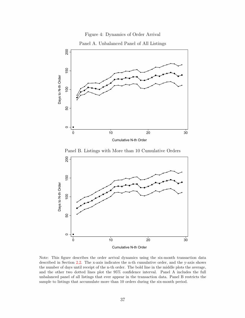
Figure 4: Dynamics of Order Arrival

Panel A. Unbalanced Panel of All Listings

050

100

150

200

Day

s to

N-th

Ord

er

0 10 20 30

Cumulative N-th Order

Panel B. Listings with More than 10 Cumulative Orders

050

100

150

200

Day

s to

N-th

Ord

er

0 10 20 30

Cumulative N-th Order

Note: This figure describes the order arrival dynamics using the six-month transaction datadescribed in Section 2.2. The x-axis indicates the n-th cumulative order, and the y-axis showsthe number of days until receipt of the n-th order. The bold line in the middle plots the average,and the other two dotted lines plot the 95% confidence interval. Panel A includes the fullunbalanced panel of all listings that ever appear in the transaction data. Panel B restricts thesample to listings that accumulate more than 10 orders during the six-month period.

37

Figure 5: Model Simulation

Panel A. Simulated Expected Quality of the Chosen Seller over Time

Panel B. Simulated Visibility Distribution over Quality

Note: This figure presents the simulation results from our counterfactual exercise of re-ducing the number of listings. Panel A plots the expected quality of the chosen seller overtime. Panel B plots the distribution of visibility over quality bins in the last simulationperiod. Data are simulated based on our baseline parameter estimates in Table 5.

38

Table 1: Summary Statistics of the Children’s T-Shirt Market on AliExpress

Observations Mean Std Dev Median 5th Pctile 95th Pctile

Panel A. Listing Level

Price 10089 6.14 8.46 5 2.78 11.59Orders 10089 31.07 189.19 2 0 110Revenue 10089 163.7 891.68 9 0 636.4Total Feedback 10089 19.69 127 1 0 67Rating 5050 96.66 7.4 100 82.9 100Free Shipping Indicator 10089 .54 .5 1 0 1Shipping Cost to US 10089 .63 1.44 0 0 2.18

Panel B. Store Level

Age 1291 1.61 1.77 1 0 5T-shirts Orders 1291 235.2 969.81 23 0 1076T-shirts Revenue 1291 1232.05 4786.45 132.47 0 5649.28Shop Rating 1218 4.73 .13 4.7 4.5 4.9

Note: This table reports the summary statistics for the children’s T-shirt market on AliExpress based on the store-listing-leveldata described in Section 2.2. Panel A reports the summary statistics at the listing level. Panel B reports the summary statisticsat the store level for stores carrying these listings. Listing and store-level ratings are only available for those with reviews.

39

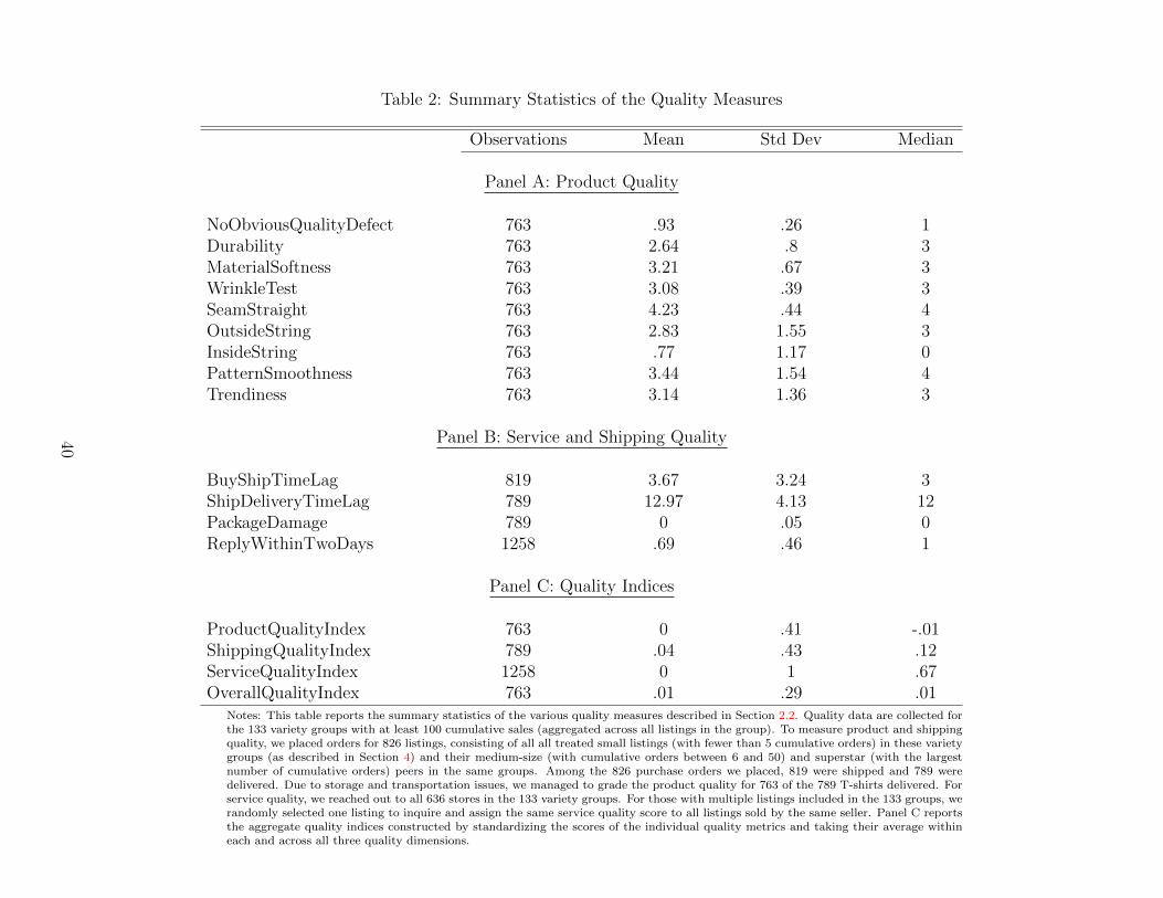
Table 2: Summary Statistics of the Quality Measures

Observations Mean Std Dev Median

Panel A: Product Quality

NoObviousQualityDefect 763 .93 .26 1Durability 763 2.64 .8 3MaterialSoftness 763 3.21 .67 3WrinkleTest 763 3.08 .39 3SeamStraight 763 4.23 .44 4OutsideString 763 2.83 1.55 3InsideString 763 .77 1.17 0PatternSmoothness 763 3.44 1.54 4Trendiness 763 3.14 1.36 3

Panel B: Service and Shipping Quality

BuyShipTimeLag 819 3.67 3.24 3ShipDeliveryTimeLag 789 12.97 4.13 12PackageDamage 789 0 .05 0ReplyWithinTwoDays 1258 .69 .46 1

Panel C: Quality Indices

ProductQualityIndex 763 0 .41 -.01ShippingQualityIndex 789 .04 .43 .12ServiceQualityIndex 1258 0 1 .67OverallQualityIndex 763 .01 .29 .01

Notes: This table reports the summary statistics of the various quality measures described in Section 2.2. Quality data are collected forthe 133 variety groups with at least 100 cumulative sales (aggregated across all listings in the group). To measure product and shippingquality, we placed orders for 826 listings, consisting of all all treated small listings (with fewer than 5 cumulative orders) in these varietygroups (as described in Section 4) and their medium-size (with cumulative orders between 6 and 50) and superstar (with the largestnumber of cumulative orders) peers in the same groups. Among the 826 purchase orders we placed, 819 were shipped and 789 weredelivered. Due to storage and transportation issues, we managed to grade the product quality for 763 of the 789 T-shirts delivered. Forservice quality, we reached out to all 636 stores in the 133 variety groups. For those with multiple listings included in the 133 groups, werandomly selected one listing to inquire and assign the same service quality score to all listings sold by the same seller. Panel C reportsthe aggregate quality indices constructed by standardizing the scores of the individual quality metrics and taking their average withineach and across all three quality dimensions.

40

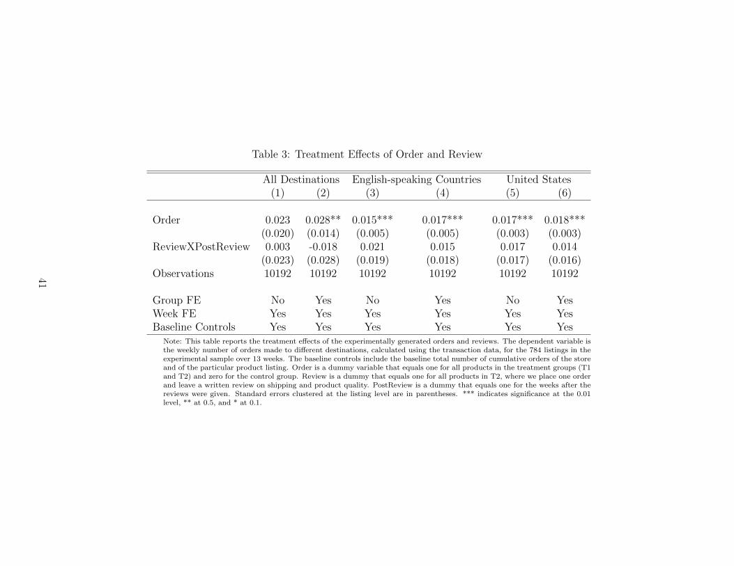
Table 3: Treatment Effects of Order and Review

All Destinations English-speaking Countries United States(1) (2) (3) (4) (5) (6)

Order 0.023 0.028** 0.015*** 0.017*** 0.017*** 0.018***(0.020) (0.014) (0.005) (0.005) (0.003) (0.003)

ReviewXPostReview 0.003 -0.018 0.021 0.015 0.017 0.014(0.023) (0.028) (0.019) (0.018) (0.017) (0.016)

Observations 10192 10192 10192 10192 10192 10192

Group FE No Yes No Yes No YesWeek FE Yes Yes Yes Yes Yes YesBaseline Controls Yes Yes Yes Yes Yes Yes

Note: This table reports the treatment effects of the experimentally generated orders and reviews. The dependent variable isthe weekly number of orders made to different destinations, calculated using the transaction data, for the 784 listings in theexperimental sample over 13 weeks. The baseline controls include the baseline total number of cumulative orders of the storeand of the particular product listing. Order is a dummy variable that equals one for all products in the treatment groups (T1and T2) and zero for the control group. Review is a dummy that equals one for all products in T2, where we place one orderand leave a written review on shipping and product quality. PostReview is a dummy that equals one for the weeks after thereviews were given. Standard errors clustered at the listing level are in parentheses. *** indicates significance at the 0.01level, ** at 0.5, and * at 0.1.

41

Table 4: Average Treatment Effects Measured at the Endline

All Destinations English-speaking Countries United States(1) (2) (3)

Order 0.096 0.186** 0.245***(0.309) (0.093) (0.063)

Review 0.444 0.078 -0.006(0.331) (0.100) (0.068)

Observations 784 784 784Baseline Controls Yes Yes Yes

Note: This table reports the average treatment effects of order and review treatment. The dependent variable isthe endline number of cumulative orders net of the experimentally generated one, calculated using the transactiondata collected in August 2018. Order is a dummy variable that equals one for all products in the treatment groups(T1 and T2) and zero for the control group. Review is a dummy that equals one for all products in T2, wherewe place one order and leave a written review on shipping and product quality. The baseline controls include thebaseline total number of cumulative orders of the store and of the particular product listing. Column (1) reportsthe average treatment effect measured by the number of orders that the listing receives from all destinations.In contrast, Column (2) and (3) consider only orders from English-speaking countries and the United States,respectively. Standard errors are in parentheses. *** indicates significance at the 0.01 level, ** at 0.5, and * at0.1.

42

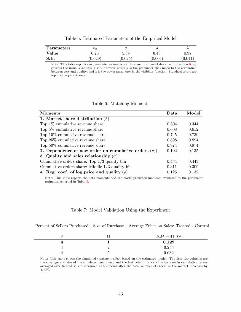
Table 5: Estimated Parameters of the Empirical Model

Parameters v0 σ ρ λValue 0.26 5.39 0.48 0.97S.E. (0.029) (0.025) (0.006) (0.011)

Note: This table reports our parameter estimates for the structural model described in Section 6. v0governs the initial visibility; σ is the review noise; ρ is the parameter that maps to the correlationbetween cost and quality; and λ is the power parameter in the visibility function. Standard errors arereported in parentheses.

Table 6: Matching Moments

Moments Data Model

1. Market share distribution (λ)Top 1% cumulative revenue share 0.304 0.344Top 5% cumulative revenue share 0.608 0.612Top 10% cumulative revenue share 0.745 0.739Top 25% cumulative revenue share 0.898 0.894Top 50% cumulative revenue share 0.974 0.9742. Dependence of new order on cumulative orders (v0) 0.102 0.1353. Quality and sales relationship (σ)Cumulative orders share: Top 1/3 quality bin 0.434 0.443Cumulative orders share: Middle 1/3 quality bin 0.311 0.3094. Reg. coef. of log price and quality (ρ) 0.125 0.132

Note: This table reports the data moments and the model-predicted moments evaluated at the parameterestimates reported in Table 5.

Table 7: Model Validation Using the Experiment

Percent of Sellers Purchased Size of Purchase Average Effect on Sales: Treated - Control

P O ∆M = 41.9%

4 1 0.1294 2 0.2554 5 0.632

Note: This table shows the simulated treatment effect based on the estimated model. The first two columns arethe coverage and size of the simulated treatment, and the last column reports the increase in cumulative ordersaveraged over treated sellers measured at the point after the total number of orders in the market increases by41.9%.

43

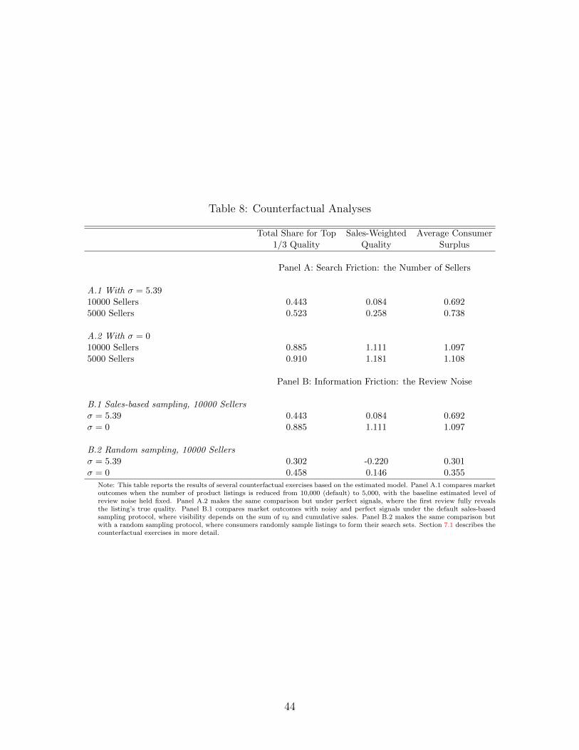
Table 8: Counterfactual Analyses

Total Share for Top Sales-Weighted Average Consumer1/3 Quality Quality Surplus

Panel A: Search Friction: the Number of Sellers

A.1 With σ = 5.3910000 Sellers 0.443 0.084 0.6925000 Sellers 0.523 0.258 0.738

A.2 With σ = 010000 Sellers 0.885 1.111 1.0975000 Sellers 0.910 1.181 1.108

Panel B: Information Friction: the Review Noise

B.1 Sales-based sampling, 10000 Sellersσ = 5.39 0.443 0.084 0.692σ = 0 0.885 1.111 1.097

B.2 Random sampling, 10000 Sellersσ = 5.39 0.302 -0.220 0.301σ = 0 0.458 0.146 0.355

Note: This table reports the results of several counterfactual exercises based on the estimated model. Panel A.1 compares marketoutcomes when the number of product listings is reduced from 10,000 (default) to 5,000, with the baseline estimated level ofreview noise held fixed. Panel A.2 makes the same comparison but under perfect signals, where the first review fully revealsthe listing’s true quality. Panel B.1 compares market outcomes with noisy and perfect signals under the default sales-basedsampling protocol, where visibility depends on the sum of v0 and cumulative sales. Panel B.2 makes the same comparison butwith a random sampling protocol, where consumers randomly sample listings to form their search sets. Section 7.1 describes thecounterfactual exercises in more detail.

44

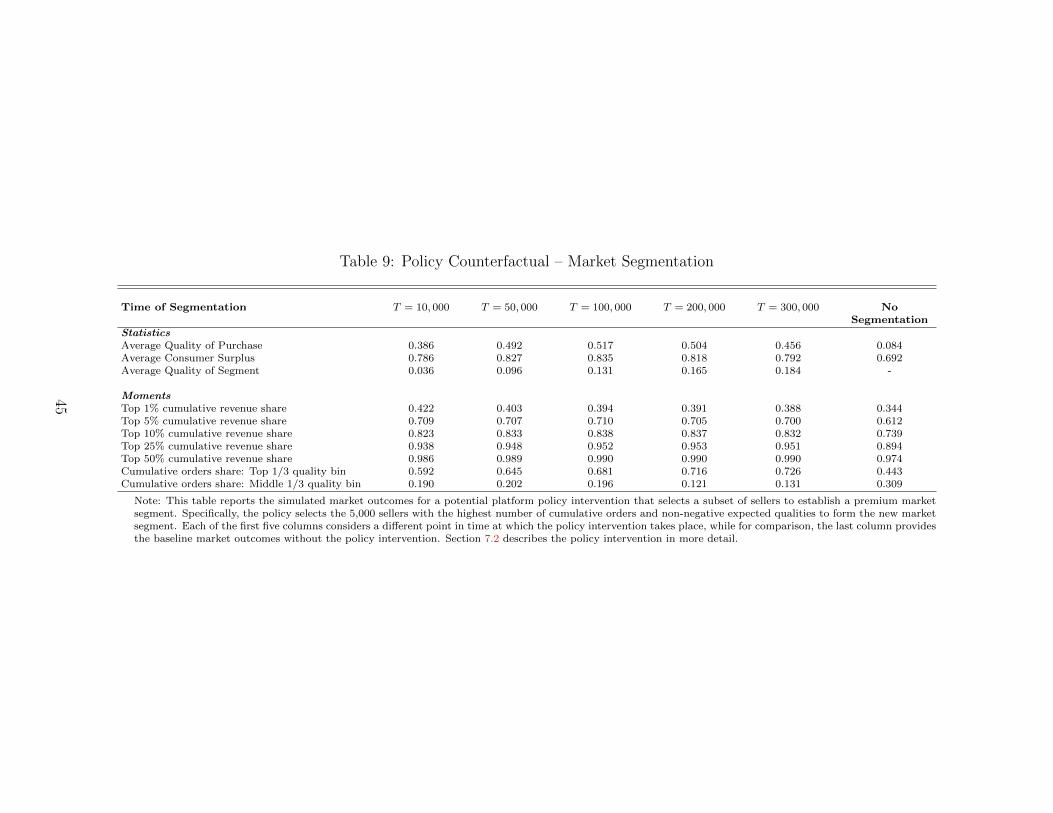
Table 9: Policy Counterfactual – Market Segmentation

Time of Segmentation T = 10, 000 T = 50, 000 T = 100, 000 T = 200, 000 T = 300, 000 NoSegmentation

StatisticsAverage Quality of Purchase 0.386 0.492 0.517 0.504 0.456 0.084Average Consumer Surplus 0.786 0.827 0.835 0.818 0.792 0.692Average Quality of Segment 0.036 0.096 0.131 0.165 0.184 -

MomentsTop 1% cumulative revenue share 0.422 0.403 0.394 0.391 0.388 0.344Top 5% cumulative revenue share 0.709 0.707 0.710 0.705 0.700 0.612Top 10% cumulative revenue share 0.823 0.833 0.838 0.837 0.832 0.739Top 25% cumulative revenue share 0.938 0.948 0.952 0.953 0.951 0.894Top 50% cumulative revenue share 0.986 0.989 0.990 0.990 0.990 0.974Cumulative orders share: Top 1/3 quality bin 0.592 0.645 0.681 0.716 0.726 0.443Cumulative orders share: Middle 1/3 quality bin 0.190 0.202 0.196 0.121 0.131 0.309

Note: This table reports the simulated market outcomes for a potential platform policy intervention that selects a subset of sellers to establish a premium marketsegment. Specifically, the policy selects the 5,000 sellers with the highest number of cumulative orders and non-negative expected qualities to form the new marketsegment. Each of the first five columns considers a different point in time at which the policy intervention takes place, while for comparison, the last column providesthe baseline market outcomes without the policy intervention. Section 7.2 describes the policy intervention in more detail.

45

Appendices. For Online Publication Only

A Figures and Tables

Figure A.1: Product Quality Measurement

Panel A. Inspection and Grading

Quality Metrics:

➢ Obvious Quality Defect (dummy)

➢ Fabric/Materials (1-5 Rating) :✓ Durability/ Strength(tightly woven?) ✓ Softness✓ Wrinkle test

➢ Seam (1-5 Rating):✓ Straight and neat (e.g. armpit) ✓ Outside stray threads ✓ Inside multiple unnecessary/loose stitches

➢ Pattern Printing (1-5 Rating):✓ Smoothness✓ Trendiness (subjective)

Panel B. Variation in Scores

Varying degrees of Durability

Failed wrinkle test

Stray threads

Poor softness

Varying quality within a variety group

A-1

Figure A.2: Sales Performance within Identical Varieties By Country

0.2

.4.6

.81

Tota

l Ord

ers

Shar

es

United States of America

Superstar Top 25%

.2.4

.6.8

1To

tal O

rder

s Sh

ares

Russian Federation

Superstar Top 25%

Note: This figure plots the distribution of within-group market shares, measured in cumulative orders,of the top listings in a group by country. The number of cumulative orders is constructed from thetransaction data from March to August 2018, in which we observe the buyer’s country of origin.Superstar indicates the listing that has the highest number of cumulative orders within its group fora given country. Top 25% indicates listings in the top 25th percentile in terms of cumulative orders.We limit the sample to groups with at least 4 listings in total and at least 1 listing with positive salesto a given country.

A-2

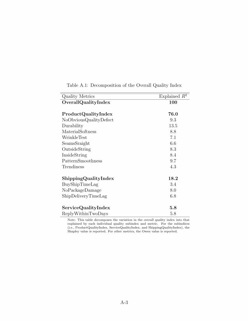
Table A.1: Decomposition of the Overall Quality Index

Quality Metrics Explained R2

OverallQualityIndex 100

ProductQualityIndex 76.0NoObviousQualityDefect 9.3Durability 13.5MaterialSoftness 8.8WrinkleTest 7.1SeamsSraight 6.6OutsideString 8.3InsideString 8.4PatternSmoothness 9.7Trendiness 4.3

ShippingQualityIndex 18.2BuyShipTimeLag 3.4NoPackageDamage 8.0ShipDeliveryTimeLag 6.8

ServiceQualityIndex 5.8ReplyWithinTwoDays 5.8

Note: This table decomposes the variation in the overall quality index into thatexplained by each individual quality subindex and metric. For the subindices(i.e., ProductQualityIndex, ServiceQualityIndex, and ShippingQualityIndex), theShapley value is reported. For other metrics, the Owen value is reported.

A-3

Table A.2: Correlation between Quality and Online Rating

Dependent: Star Rating(1) (2) (3) (4) (5) (6)

ProductQualityIndex 0.030 0.170(0.048) (0.114)

ShippingQualityIndex 0.081* 0.098*(0.044) (0.056)

ServiceQualityIndex 0.034** 0.036*(0.017) (0.020)

Constant 4.802*** 4.804*** 4.794*** 4.793*** 4.793*** 4.793***(0.019) (0.020) (0.019) (0.020) (0.016) (0.017)

Observations 408 408 421 421 624 624Rsquare 0.001 0.316 0.008 0.318 0.006 0.210Group FE No Yes No Yes No Yes

Note: This table presents the results from regressing listings’ star ratings on the three quality indices. The number of observationsin each column reflects the number of listings with non-missing quality indices and star rating. Standard errors are in parentheses.*** indicates significance at the 0.01 level, ** at 0.5, and * at 0.1.

Table A.3: Consistency of Service Quality Over Time

Measured 2nd and 3rd roundsReply (dummy) Reply within 2 days (dummy) Hours to reply

Measured in 1st round (1) (2) (3)Reply (dummy) 0.614***

(0.058)Reply within 2 days (dummy) 0.562***

(0.059)Hours to reply 0.591***

(0.060)Constant 0.231*** 0.259*** 26.769***

(0.052) (0.052) (4.094)Observations 264 264 264

Note: This table presents the results from regressing the seller’s reply behavior in the second and third rounds (stacked) on itsbehavior in the first round. The data consist of the 132 stores visited in June 2021, for which we collected three rounds of servicequality data. Standard errors are in parentheses. *** indicates significance at the 0.01 level, ** at 0.5, and * at 0.1.

Table A.4: Dependence of New Order Arrival on Cumulative Orders

Dummy=1 if having an order in the following week (1) (2)Log Orders 0.092*** 0.102***

(0.001) (0.002)Observations 15096 15096Store FE No Yes

Note: This table reports the results from regressing a dummy variable that equals one for listingsthat receive orders in the following week on the log number of cumulative orders in the current week.The data consists of a weekly panel of 1258 listings over 12 weeks (corresponding to the interventionperiod from May to August 2018 as described in Section 4). The weekly panel is constructed basedon the six-month transaction data described in Section 2.2.

A-4

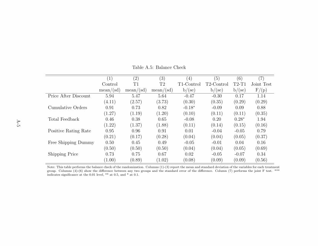
Table A.5: Balance Check

(1) (2) (3) (4) (5) (6) (7)Control T1 T2 T1-Control T2-Control T2-T1 Joint Test

mean/(sd) mean/(sd) mean/(sd) b/(se) b/(se) b/(se) F/(p)Price After Discount 5.94 5.47 5.64 -0.47 -0.30 0.17 1.14

(4.11) (2.57) (3.73) (0.30) (0.35) (0.29) (0.29)Cumulative Orders 0.91 0.73 0.82 -0.18∗ -0.09 0.09 0.88

(1.27) (1.19) (1.20) (0.10) (0.11) (0.11) (0.35)Total Feedback 0.46 0.38 0.65 -0.08 0.20 0.28∗ 1.94

(1.22) (1.37) (1.88) (0.11) (0.14) (0.15) (0.16)Positive Rating Rate 0.95 0.96 0.91 0.01 -0.04 -0.05 0.79

(0.21) (0.17) (0.28) (0.04) (0.04) (0.05) (0.37)Free Shipping Dummy 0.50 0.45 0.49 -0.05 -0.01 0.04 0.16

(0.50) (0.50) (0.50) (0.04) (0.04) (0.05) (0.69)Shipping Price 0.73 0.75 0.67 0.02 -0.05 -0.07 0.34

(1.00) (0.89) (1.02) (0.08) (0.09) (0.09) (0.56)

Note: This table performs the balance check of the randomization. Columns (1)-(3) report the mean and standard deviation of the variables for each treatmentgroup. Columns (4)-(6) show the difference between any two groups and the standard error of the difference. Column (7) performs the joint F test. ***indicates significance at the 0.01 level, ** at 0.5, and * at 0.1.

A-5

Table A.6: Treatment Effects of Order and Review: Without Baseline Controls

All Destinations English-speaking United StatesOrder 0.022 0.027* 0.014** 0.016*** 0.016*** 0.017***

(0.020) (0.015) (0.005) (0.005) (0.003) (0.003)ReviewXPostReview 0.006 -0.015 0.022 0.016 0.018 0.014

(0.024) (0.028) (0.019) (0.018) (0.017) (0.016)Observations 10192 10192 10192 10192 10192 10192Group FE No Yes No Yes No YesWeek FE Yes Yes Yes Yes Yes YesBaseline Controls No No No No No No

Note: This table reports the treatment effects of the experimentally generated orders and reviews without baselinecontrols. Standard errors clustered at the listing level are in parentheses. *** indicates significance at the 0.01level, ** at 0.5, and * at 0.1.

A-6

Table A.7: Treatment Effects on Ranking

(1) (2)Enter First 15 Pages

OrderXMonth1 0.004* 0.003*(0.002) (0.002)

OrderXMonth2 0.002 0.002(0.002) (0.001)

OrderXMonth3 -0.000 -0.000(0.002) (0.002)

OrderXMonth4 0.002 0.002(0.002) (0.002)

Observations 10192 10192Group FE No YesWeek FE Yes YesBaseline Controls Yes Yes

Note: This table reports the treatment effects of the ex-perimentally generated orders and reviews on a listing’sranking. The dependent variable is a dummy variablethat equals one if the listing enters the first 15 pagesof the search results (without grouping). The baselinecontrols include the baseline total number of cumula-tive orders of the store and of the particular productlisting. Order is a dummy variable that equals one forall products in the treatment groups (T1 and T2) andzero for the control group. MonthX is a dummy vari-able that equals one for the X-th month after the initialorder placement. Standard errors clustered at the list-ing level are in parentheses. *** indicates significanceat the 0.01 level, ** at 0.5, and * at 0.1.

A-7

Table A.8: Dynamic Treatment Effects

All Destinations English-speaking Countries United States

OrderXMonth1 0.063*** 0.065*** 0.037*** 0.038*** 0.038*** 0.038***(0.024) (0.021) (0.008) (0.008) (0.007) (0.007)

OrderXMonth2 0.017 0.020 0.006 0.008 0.007** 0.008**(0.032) (0.027) (0.010) (0.009) (0.003) (0.004)

OrderXMonth3 0.008 0.011 0.015* 0.016** 0.012* 0.013**(0.020) (0.017) (0.008) (0.008) (0.007) (0.006)

OrderXMonth4 -0.047 -0.044 -0.009 -0.007 0.011 0.011(0.031) (0.029) (0.019) (0.018) (0.008) (0.008)

Observations 10192 10192 10192 10192 10192 10192

Group FE No Yes No Yes No YesWeek FE Yes Yes Yes Yes Yes YesBaseline Controls Yes Yes Yes Yes Yes Yes

Note: This table reports the dynamic treatment effects of the experimentally generated orders and reviews. The dependentvariable is the weekly number of orders. The baseline controls include the baseline total number of cumulative orders of thestore and of the particular product listing. MonthX is a dummy variable that equals one for the X-th month after initialorder placement. Standard errors clustered at the listing level are in parentheses. *** implies significance at the 0.01 level,** at 0.5, and * at 0.1.

A-8

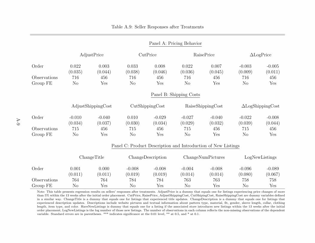
Table A.9: Seller Responses after Treatments

Panel A: Pricing Behavior

AdjustPrice CutPrice RaisePrice ∆LogPrice

Order 0.022 0.003 0.033 0.008 0.022 0.007 -0.003 -0.005(0.035) (0.044) (0.038) (0.046) (0.036) (0.045) (0.009) (0.011)

Observations 716 456 716 456 716 456 716 456Group FE No Yes No Yes No Yes No Yes

Panel B: Shipping Costs

AdjustShippingCost CutShippingCost RaiseShippingCost ∆LogShippingCost

Order -0.010 -0.040 0.010 -0.029 -0.027 -0.040 -0.022 -0.008(0.034) (0.037) (0.030) (0.034) (0.029) (0.032) (0.039) (0.044)

Observations 715 456 715 456 715 456 715 456Group FE No Yes No Yes No Yes No Yes

Panel C: Product Description and Introduction of New Listings

ChangeTitle ChangeDescription ChangeNumPictures LogNewListings

Order 0.001 0.000 -0.008 -0.008 -0.004 -0.008 -0.096 -0.089(0.011) (0.011) (0.019) (0.019) (0.014) (0.014) (0.080) (0.067)

Observations 764 764 784 784 763 763 758 758Group FE No Yes No Yes No Yes No Yes

Note: This table presents regression results on sellers’ responses after treatments. AdjustPrice is a dummy that equals one for listings experiencing price changes of morethan 5% within the 13 weeks after the initial order placement. CutPrice, RaisePrice, AdjustShippingCost, CutShipingCost, RaiseShippingCost are dummy variables definedin a similar way. ChangeTitle is a dummy that equals one for listings that experienced title updates. ChangeDescription is a dummy that equals one for listings thatexperienced description updates. Descriptions include website pictures and textual information about pattern type, material, fit, gender, sleeve length, collar, clothinglength, item type, and color. HaveNewListings is dummy that equals one for a listing if the associated store introduces new listings within the 13 weeks after the initialorder placement; LogNewListings is the log number of those new listings. The number of observations in each column reflects the non-missing observations of the dependentvariable. Standard errors are in parentheses. *** indicates significance at the 0.01 level, ** at 0.5, and * at 0.1.

A-9

Table A.10: Heterogeneous Treatment Effects Based on Quality

(1) (2) (3) (4)Order 0.301 0.327* -0.489 -0.676

(0.236) (0.180) (0.624) (0.509)OrderXServiceQualityIndex -0.157 -0.075

(0.228) (0.203)ServiceQualityIndex 0.290** 0.093

(0.119) (0.125)OrderXStarRating -0.715 -0.691

(0.816) (0.755)StarRating -0.122 0.202

(0.392) (0.428)Observations 784 784 307 307Baseline Controls Yes Yes Yes YesGroup FE No Yes No Yes

Note: This table reports the heterogeneous treatment effects of the experimentally generated orders based on quality measures.The dependent variable is the endline number of cumulative orders net of the experimentally generated one. The fewer numbersof observations in Columns (3) and (4) reflect the fact that some listings have not received any rating. The baseline controlsinclude the baseline total number of cumulative orders of the store and of the particular product listing. Order is a dummyvariable that equals one for all products in the treatment groups (T1 and T2) and zero for the control group. Standard errorsare in the parentheses. *** indicates significance at the 0.01 level, ** at 0.5, and * at 0.1.

A-10

Table A.11: Robustness: Structural Estimation

(1) (2) (3) (4) (5) (6)Data Baseline Sampling Alternative Smaller Larger

Without Sample Price PriceA. Parameter Estimates Replacement Size Elasticity Elasticity

Initial Visibility v0 0.26 0.26 0.25 0.25 0.25Review Noisiness σ 5.39 5.39 7.01 6.03 5.80Quality-Cost Correlation ρ 0.48 0.48 0.45 0.45 0.45Strength of Demand Reinforcement λ 0.97 0.97 0.94 0.96 0.96B. Simulated vs. Data Moments

Market share distributionTop 1% cumulative revenue share 0.304 0.344 0.340 0.346 0.327 0.345Top 5% cumulative revenue share 0.608 0.612 0.608 0.604 0.596 0.606Top 10% cumulative revenue share 0.745 0.739 0.737 0.732 0.728 0.734Top 25% cumulative revenue share 0.898 0.894 0.894 0.891 0.890 0.893Top 50% cumulative revenue share 0.974 0.974 0.973 0.973 0.973 0.973Dependence of new order on cumulative orders 0.102 0.135 0.135 0.137 0.137 0.136Quality and sales relationshipCumulative orders share: Top 1/3 quality bin 0.434 0.443 0.443 0.422 0.435 0.458Cumulative orders share: Middle 1/3 quality bin 0.311 0.309 0.305 0.312 0.310 0.298Reg. coef. of log price and quality 0.125 0.132 0.132 0.124 0.131 0.112

Note: This table reports the parameter estimates and model fitness in the baseline and alternative model calibrations. Column (2) reproduces the baseline resultsin Tables 5 and 6. Column (3) simulates the model moments under the baseline parameter values based on sampling without replacement for the formation ofconsumers’ search samples. Column (4) assumes that the consumer search sample size K follows a positive Poisson distribution with mean 5. Column (5) assumesthat the price elasticity is 4 or, equivalently, that γ is 0.75. Finally, Column (6) sets the price elasticity to 10, where γ equals 1.89.

A-11

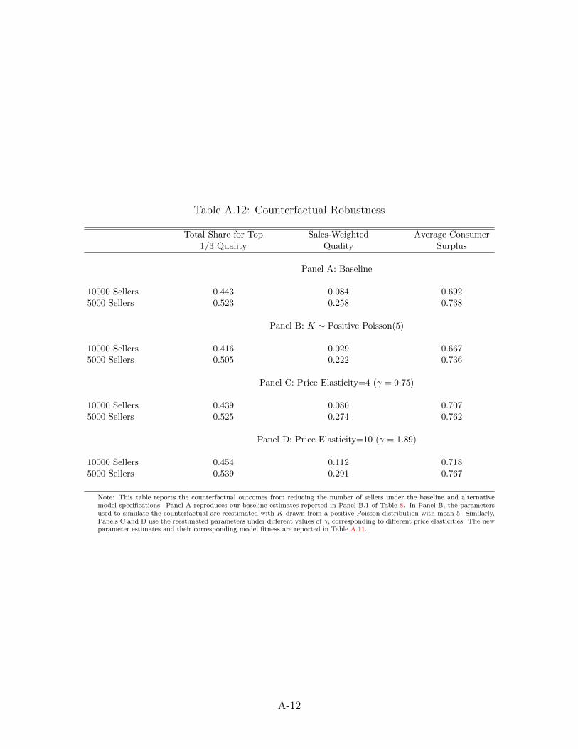
Table A.12: Counterfactual Robustness

Total Share for Top Sales-Weighted Average Consumer1/3 Quality Quality Surplus

Panel A: Baseline

10000 Sellers 0.443 0.084 0.6925000 Sellers 0.523 0.258 0.738

Panel B: K ∼ Positive Poisson(5)

10000 Sellers 0.416 0.029 0.6675000 Sellers 0.505 0.222 0.736

Panel C: Price Elasticity=4 (γ = 0.75)

10000 Sellers 0.439 0.080 0.7075000 Sellers 0.525 0.274 0.762

Panel D: Price Elasticity=10 (γ = 1.89)

10000 Sellers 0.454 0.112 0.7185000 Sellers 0.539 0.291 0.767

Note: This table reports the counterfactual outcomes from reducing the number of sellers under the baseline and alternativemodel specifications. Panel A reproduces our baseline estimates reported in Panel B.1 of Table 8. In Panel B, the parametersused to simulate the counterfactual are reestimated with K drawn from a positive Poisson distribution with mean 5. Similarly,Panels C and D use the reestimated parameters under different values of γ, corresponding to different price elasticities. The newparameter estimates and their corresponding model fitness are reported in Table A.11.

A-12

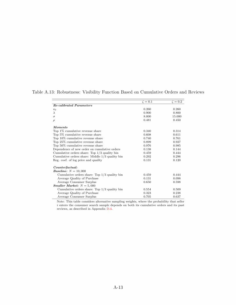
Table A.13: Robustness: Visibility Function Based on Cumulative Orders and Reviews

ζ = 0.1 ζ = 0.2Re-calibrated Parametersv0 0.260 0.260λ 0.900 0.800σ 8.000 15.000ρ 0.481 0.450

MomentsTop 1% cumulative revenue share 0.340 0.314Top 5% cumulative revenue share 0.608 0.611Top 10% cumulative revenue share 0.740 0.761Top 25% cumulative revenue share 0.899 0.927Top 50% cumulative revenue share 0.976 0.985Dependence of new order on cumulative orders 0.138 0.144Cumulative orders share: Top 1/3 quality bin 0.459 0.444Cumulative orders share: Middle 1/3 quality bin 0.292 0.296Reg. coef. of log price and quality 0.131 0.120

Counterfactual:Baseline: N = 10, 000

Cumulative orders share: Top 1/3 quality bin 0.459 0.444Average Quality of Purchase 0.131 0.098Average Consumer Surplus 0.650 0.598

Smaller Market: N = 5, 000Cumulative orders share: Top 1/3 quality bin 0.554 0.509Average Quality of Purchase 0.323 0.238Average Consumer Surplus 0.705 0.637

Note: This table considers alternative sampling weights, where the probability that selleri enters the consumer search sample depends on both its cumulative orders and its pastreviews, as described in Appendix D.4.

A-13

B Data and the Experiment

B.1 Additional Details on Measuring Product and Service Quality

Product Quality. We worked with a large local consignment store of children’s clothing in

North Carolina to inspect and grade the quality of each T-shirt. The owner has over 30 years of

experience in the retail clothing business. Each T-shirt was given an anonymous identification

number, and the owner was asked to grade the T-shirt on 8 quality dimensions, following standard

grading criteria used in the textile and garment industry, as shown in Panel A of Figure A.1.

In addition, the examiner was asked to price each T-shirt based on her willingness to pay and

willingness to sell, respectively. T-shirts within the same variety were grouped together for

assessment to make sure that the grading could capture within-variety variations. The examiner

conducted two rounds of evaluation that took place several weeks apart to ensure consistency in

grading.

Service Quality. To measure service quality, the following message was sent to sellers via the

platform:

“Hi, I am wondering if you could help me choose a size that fits my kid, who is 5 years old, 45

lbs and about 4 feet. I would also like to know a bit more about the quality of the T-shirt. Are

the colors as shown in the picture? Will it fade after washing? What is the material content, by

the way? Does it contain 100% cotton? The order is a little urgent; how soon can you send the

good? Would it be possible to expedite the shipping, and how much would that cost? Thanks in

advance!”

B.2 Review Treatment

To generate the content of the reviews, we use the latent Dirichlet allocation topic model in

natural language processing to analyze past reviews and construct the messages based on the

identified keywords. Specifically, the following reviews were provided (randomly) to listings in

T2:

Product Quality:

• “Great shirt! Soft, dense material, quality is good; color matching the picture exactly, and

I am happy with the design; no problem after washing. My kid really likes it. Thank you!”

• “Well-made shirt. It was true to size. The material was very soft and smooth. My kid

really likes the design. I am overall satisfied with it.”

B-14

• “This shirt is nice and as seen in the photo. It fits my kid pretty well. The material is

quite sturdy and colorfast after washing.”

Shipping Quality:

• “The shipping was pretty good. Package arrived within the estimated amount of time and

appeared intact on my porch.”

• “I am pleased with the shipping. It was fast and easily trackable online. The delivery was

right on time, and the package appeared without any scratches.”

• “Fast delivery and convenient pickup, everything is smooth, shirt came in a neat package,

not wrinkled. Thank you!”

We left positive reviews on all listings unless there were obvious quality defects or shipping

problems, in which case no review was provided.

B-15

C Theory Appendix

C.1 Proof of Proposition 1

Since the full proof below is technically involved, we first explain the simple intuition here. The

key observation is that for a consumer to obtain higher quality than expected under her prior, it

is necessary that she sample a seller chosen in previous periods so as to benefit from past reviews.

In light of this feature, expected quality is related to the probability of resampling a seller. In

early periods, this probability is proportional to 1N

and thus decreases with the number N of

sellers.

Turning to the formal proof, it suffices to study the expected quality in period T . We compute

this expectation by adopting the subjective perspective, which involves averaging across different

histories the belief in period T − 1 about the seller’s quality in period T . By the law of iterated

expectations, this average is indeed the ex ante expected quality.

Notice that each possible history of the first T periods can be described by the following:

• the search sample (i1t , . . . , iKt ) in each period 1 ≤ t ≤ T ;

• an index k(t) ∈ {1, . . . , K} in each period 1 ≤ t ≤ T describing which of the K sellers is

chosen out of the sample;

• conditionally independent signal realizations zt about the true quality of seller ik(t)t chosen

in each period t, where zt = qik(t)t +N (0, σ2).

These variables, which we denote by H, are sufficient to pin down the evolution of sales {sit} and

beliefs qit. It turns out to be convenient to ignore the last variables k(T ) and zT and compute

the expected quality in period T conditional on what happens before a choice is made in period

T . Thus, in what follows, when we refer to a “history,” we exclude k(T ) and zT .

Crucially, the likelihood of any such history can be explicitly written as the following product:

L(H) =

(T∏t=1

K∏k=1

(v0 + siktt−1)λ∑N

j=1(v0 + sjt−1)λ

)·

T−1∏t=1

exp(qik(t)tt−1 )∑K

k=1 exp(qiktt−1)

· l (z1, . . . , zT−1 | {ik(t)t }t≤T−1

).

(C.1)

The first multiplicative factor above captures the probability of generating each K-sample (based

on initial visibility and sales). The second factor is the probability of choosing the particular seller

out of the sample (based on the logit rule applied to beliefs). The last factor, l(z1, . . . , zt−1 | ·),represents the probability of seeing the signal realizations zt (based on the normal prior and

signals). The product of these factors is the likelihood of a given history, which is the weight

that we use to average across different histories.

C-16

Note also that given H, the believed quality of the seller chosen in period T is completely

determined by the sample (i1T , . . . , iKT ) in period T and the beliefs about these sellers at the end

of period T − 1. This believed quality can be written as

f(H) =K∑j=1

qijTT−1 ·

exp(qijTT−1)∑K

k=1 exp(qikTT−1)

. (C.2)

Hence, the ex ante expected quality in period T can be computed as the integral∫f(H) · L(H) dH.

Below, we decompose this integral into 3 parts, corresponding to 3 different kinds of histories H:

(1) First, consider any historyH where all sellers sampled in period T have not been previously

chosen (i.e., ijT 6= ik(t)t for all j and all t < T ). In this case, all these sellers are believed

to have expected quality 0, just as in the prior. It follows that f(H) = 0, and so we can

ignore such histories in computing the above integral.

(2) We then consider histories where all K · (T −1) sellers sampled before period T are distinct

but there is a unique seller sampled in period T that coincides with a previously chosen

seller. The other K − 1 sellers sampled in period T are all distinct from the previously

sampled K · (T − 1) and distinct from each other.

Ignoring the signals for the moment, the total likelihood/probability of generating samples

of this form isK(T − 1)(v0 + 1)λ

(∏KT−2s=0 (N − s)(v0)λ

)∏T

t=1((N − t+ 1)(v0)λ + (t− 1)(v0 + 1)λ)K.

To understand this expression, note that for the sample in period 1 to consist of distinct

sellers, we can arbitrarily draw i11 but can only draw i21 with probability (N−1)(v0)λ

N(v0)λ, i31 with

probability (N−2)(v0)λ

N(v0)λand so on. Similar conditional probabilities apply to all sampled

sellers before period T and to all but one of the sellers sampled in period T . The remaining

term K(T−1)(v0+1)λ

(N−T+1)(v0)λ+(T−1)(v0+1)λin the above expression is the probability of the only seller

sampled in period T that repeats a previously chosen seller—K here is the possible positions

of this seller in the period T sample, T − 1 is the number of previously chosen sellers that

can be repeated, and v0 + 1 is the visibility of a previously chosen seller.34

34In this probability calculation, we do not worry about k(t), the positions of the previously chosen sellers. Thisis without loss because we assume that the sellers sampled before period T are all distinct and thus completelysymmetric.

C-17

We now take into account the signals before period T . Only one of those signals is relevant

for what happens in period T , and that is the signal about the particular seller i that

is repeated in the period T sample. This signal z = qi + N (0, σ2) leads to the belief

qiT−1 = z1+σ2 by Bayes’s rule. Since qi ∼ N (0, 1), it is easy to see that the ex ante

distribution of the belief qiT−1 is normal with mean 0 and variance 11+σ2 . For the remaining

K − 1 sellers sampled in period T , their beliefs are zero, as in the prior.

Thus, given the samples and the belief q = qiT−1 about the special seller i, the believed

quality in period T can be computed as f(H) = q · exp(q)K−1+exp(q)

. Integrating over q, we obtain

that given any collection of samples in the first T periods that repeat only one seller (in

period T ), the believed quality in period T is

η = E[q · exp(q)

K − 1 + exp(q)| q ∼ N (0,

1

1 + σ2)

]> 0.

This is positive because q · exp(q)K−1+exp(q)

+ (−q) · exp((−q))K−1+exp((−q)) > 0 whenever q 6= 0.

To summarize, for samples in the first T periods that have the “repeat only once” property,

their contribution to the expected quality in period T is

η ·K(T − 1)(v0 + 1)λ

(∏KT−2s=0 (N − s)(v0)λ

)∏T

t=1((N − t+ 1)(v0)λ + (t− 1)(v0 + 1)λ)K.

The specific expression does not matter; what is important is that we can rewrite this

contribution asP (N)

Q(N)

for some polynomials P and Q with positive leading coefficients and degrees KT − 1 and

KT , respectively. This ratio formalizes the intuitive idea that the probability of repeating

one seller in the samples is on the order of 1N

.

(3) In all remaining histories, the KT sellers sampled in the first T periods represent at most

KT − 2 distinct sellers (i.e., there are at least two repetitions in the samples). We show

that the contribution of these histories to the period T expected quality can be written as

a finite sum of ratios ∑m

Rm(N)

Sm(N),

where each Rm(N) is a polynomial with degree at most KT − 2 and each Sm(N) is a

polynomial with degree KT . Again, the broad intuition is that the probability of “repeating

twice” is on the order of 1N2 .

C-18

More formally, let us consider a generic “collection” of samples {ijt}1≤j≤K,1≤t≤T and chosen

seller positions {k(t)}1≤t≤T−1, representing a set of histories in which the signal realizations

are random. If we permute the labeling of all N sellers, then the indices in the samples

are relabeled accordingly. However, due to ex ante symmetry, the resulting set of histories

makes the the same contribution to the period T expected quality as the original set. Thus,

to compute the total contribution of all possible “collections,” we just need to compute the

contributions of different collections that cannot be relabeled into each other and then

do a weighted sum with weights given by the number of relabelings associated with each

collection.

The benefit of this approach is that modulo relabeling, we are essentially concerned with the

patterns of repetition among KT sampled sellers. The number of such patterns depends

on K,T but not on N , and so does the number of collections that cannot be relabeled

into each other (the latter number is KT−1 times larger since a collection also specifies

chosen sellers). On the other hand, for any fixed collection in which the samples represent

d ≤ KT − 2 sellers, the number of possible relabelings is simply∏d−1

s=0(N − s), which is

a polynomial of degree at most KT − 2. Thus, if we could show that the contribution of

any fixed collection can be written as cS(N)

for some constant c and some polynomial S(N)

with degree KT , then the weighted sum of such contributions would have the desired form∑m

Rm(N)Sm(N)

with deg(Sm) = KT and deg(Rm) ≤ KT − 2.

Now, for a fixed collection, we know that the sales evolution has been determined. Thus,

the first part on the RHS of (C.1) is fixed and has the form c1S(N)

for some constant c1

and some polynomial S(N) with degree KT . Using (C.1) and (C.2), we can write the

contribution of this collection as

c1

S(N)·∫z1,...,zT−1

T−1∏t=1

exp(qik(t)tt−1 )∑K

k=1 exp(qiktt−1)

· l (z1, . . . , zT−1) ·

K∑j=1

qijTT−1 ·

exp(qijTT−1)∑K

k=1 exp(qikTT−1)

,

where we recall that the beliefs qit can be expressed in terms of the signal realizations zt.

The integral above is another finite constant c2 independent of N , as we desire to show.35

35To see that the integral is finite, we interpret it as the expectation of the following function of beliefs:T−1∏t=1

exp(qik(t)tt−1 )∑K

k=1 exp(qiktt−1)

× K∑j=1

qijTT−1 ·

exp(qijTT−1)∑K

k=1 exp(qikTT−1)

.

This function is bounded in absolute value by∑Kj=1 |

qijTT−1|, which has a finite expectation because the beliefs

C-19

We now put together the 3 kinds of histories studied above to prove Proposition 1. The

previous analysis allows us to deduce that the expected quality in period T can be written as

P (N)

Q(N)+∑m

Rm(N)

Sm(N).

Simple calculus shows that the derivative of P (N)Q(N)

with respect to N is negative for large N and

on the order of 1N2 (just like the derivative of 1

N). In contrast, the derivative of each Rm(N)

Sm(N)may

be positive or negative but, in either case, is at most on the order of 1N3 . Thus, the derivative of

the overall sum P (N)Q(N)

+∑

mRm(N)Sm(N)

is also negative for large N . In words, when N is sufficiently

large, the expected quality in early periods decreases with N , completing the proof.

C.2 Proof of Proposition 2: The Case of λ = 1

Throughout this proof, the true qualities are fixed such that seller 1 has the unique highest

quality, i.e., q1 > qi for every i > 1. We first make some preliminary observations. Because each

review is independent from the entire past history, the joint stochastic processes of purchases

and reviews can be disentangled such that reviews are drawn ex ante and purchase decisions

then made based on these fixed reviews and induced beliefs. To be more specific, for every seller

i, let Y i1 , Y

i2 , . . . be i.i.d. random variables with the distribution qi +N (0, σ2). We think of Y i

m

as the m-th review for seller i. These reviews generate beliefs

qit =(Y i

1 + · · ·+ Y im)/σ2

1 +m/σ2,

where t is the period in which seller i is chosen for the m-th time. Using these beliefs, the

sampling and choice procedures then iteratively determine which seller is chosen in each period.

Note that it is possible for a seller i to be chosen only finitely often along certain histories. In

these situations, some reviews Y im and the resulting beliefs are never realized, but ex ante, we

could still think of them as the reviews and beliefs that would have been realized.

Recall that we want to show that the highest quality seller 1 almost surely obtains full market

share in the long run. Thus, we can without loss focus on the probability-one event that the

time-averaged reviewY i1 +···+Y im

mconverges to the true quality qi for every seller i (by the strong law

of large numbers). It suffices to fix any such collection of reviews and show that with conditional

probability one, seller 1 obtains full market share in the long run.

Henceforth, the reviews are fixed, with the property that the time-averaged reviews converge

to the true qualities. Since the absolute value of belief qit =(Y i1 +···+Y im)/σ2

1+m/σ2 is bounded above by

qijTT−1 all have a normal distribution. Thus, the dominated function has a finite expectation as well.

C-20

the absolute value ofY i1 +···+Y im

m, and since the latter is bounded as a convergent sequence, we

deduce that all beliefs about all sellers are bounded between −M and M for some large positive

constant M .

We use this bounded-belief property to show that almost surely every seller is chosen infinitely

often. Indeed, in any period t + 1, the sampling probability of seller i isvit∑j vjt

=vit

Nv0+t≥ v0

Nv0+t.

Thus, the expected number of copies of seller i in the sample of size K is at least Kv0Nv0+t

. On the

other hand, under logit choice, each copy of seller i is chosen out of the sample with probability

at least e−M

KeM(since beliefs are bounded between −M and M). Putting it together, we know that

the choice probability of seller i in period t+ 1 is at least

Kv0

Nv0 + t· e−M

KeM=

e−2Mv0

Nv0 + t=

c

Nv0 + t

for some positive constant c. Because of this, the probability that seller i is not chosen after

some period T is at most∏

t≥T (1 − cNv0+t

) = 0, where the infinite product is zero because the

harmonic sum∑

t≥Tc

Nv0+tdiverges. Since this holds for every T , a union bound implies that

the probability that seller i is chosen only finitely many times is zero. This is what we desired

to show.

Next, as the time-averaged reviewsY i1 +···+Y im

mconverge to the true quality qi as m→∞, so do

the induced beliefs(Y i1 +···+Y im)/σ2

1+m/σ2 . Let δ be a positive number smaller than q1− qi for every i > 1.

Then, there exist positive integers m1, . . . ,mN such that at any period t when each seller i has

been chosen at least mi times, the belief difference q1t − qit between seller 1 and every other seller

is at least δ. For every positive integer T , we let HT be the set of all histories such that each

seller i is chosen at least mi times by the end of period T but not by the end of period T − 1.

Then, these events HT are disjoint and together constitute a probability-one event because each

seller is chosen infinitely often. It thus suffices to show that within each HT , seller 1’s market

share almost surely converges to one.

We are now in a position to present the main part of the proof. Based on the above analysis,

we now fix T and also fix the purchase decisions in the first T periods, with the property that

each seller i has been chosen at least mi times. Given this property, the belief difference between

seller 1 and every other seller is at least δ in all future periods, regardless of the random future

purchase decisions. We use this property to show that seller 1’s fraction of total saless1tt

converges

to one almost surely. It turns out to be more convenient to work with seller 1’s fraction of total

visibility, i.e.,

r1t =

v1t∑j v

jt

=v0 + s1

t

Nv0 + t∈ [0, 1].

C-21

This coincides with the sampling probability R1t = (v1

t )λ/∑

j(vjt )λ precisely when λ = 1.

It is easy to sees1tt→ 1 if and only if r1

t → 1 as t → ∞. To show r1t → 1, we note that the

key idea is when λ = 1, r1t is the probability of sampling seller 1 in period t+ 1. However, since

logit choice favors higher expected quality, and since seller 1 actually has the highest belief, the

probability of choosing seller 1 in period t+ 1 exceeds r1t . This then implies that in expectation

r1t+1 exceeds r1

t , making the process {r1t } a bounded submartingale. Such a process almost surely

converges, and with some additional analysis, we can show that it converges to the maximum

value of 1.

To make this argument more precise, we begin by calculating the probability of choosing

seller 1 in any period t + 1 (with t ≥ T ). Since seller 1’s expected quality exceeds that of other

sellers by at least δ, it is easy to see that in any sample of K sellers where seller 1 appears k < K

times, the logit probability of seller 1 being chosen from the sample is at least kk+(K−k)e−δ

. This

is at least (1+η)kK

for some positive constant η that depends on δ. Hence, by considering different

k and incorporating the corresponding sampling probabilities, we know that the overall choice

probability of seller 1 in period t+ 1 satisfies

p1t+1 ≥ (r1

t )K +

∑1≤k≤K−1

(K

k

)(r1t )k(1− r1

t )K−k · (1 + η)k

K

= −η(r1t )K +

∑1≤k≤K

(K

k

)(r1t )k(1− r1

t )K−k · (1 + η)k

K

= −η(r1t )K + (1 + η)r1

t

∑1≤k≤K

(K − 1

k − 1

)(r1t )k−1(1− r1

t )K−k

= −η(r1t )K + (1 + η)r1

t

≥ −η(r1t )

2 + (1 + η)r1t

= r1t (1 + η(1− r1

t )).

(C.3)

With probability p1t+1, seller 1’s visibility increases by 1, and thus r1

t+1 =v1t+1

Vt+1= rtVt+1

Vt+1, where

we define

Vt =∑j

vjt = Nv0 + t.

Otherwise, r1t+1 =

v1tVt+1

= rtVtVt+1

. Since p1t+1 ≥ r1

t as given by (C.3), it is straightforward to verify

E[r1t+1 | r1

t ] ≥ r1t , so that {r1

t } is indeed a submartingale process that converges almost surely.

However, to show that the limit is almost surely one, we in fact consider a different sub-

martingale process given by log(r1t )− 1

v1t. Its evolution is such that with probability p1

t+1, we have

log(r1t+1) − 1

v1t+1= log(

v1t+1

Vt+1) − 1

v1t+1and otherwise log(r1

t+1) − 1v1t+1

= log(v1tVt+1

) − 1v1t

. From this,

C-22

we calculate

E[log(r1t+1)− 1

v1t+1

| r1t ] = log(

v1t

Vt + 1)− 1

v1t

+ p1t+1 ·

(log(

v1t + 1

v1t

) +1

v1t (v

1t + 1)

)= log(r1

t )−1

v1t

− log(Vt + 1

Vt) + p1

t+1 ·(

log(v1t + 1

v1t

) +1

v1t (v

1t + 1)

)> log(r1

t )−1

v1t

− 1

Vt+ p1

t+1 ·1

v1t

= log(r1t )−

1

v1t

+1

Vt

(p1t+1

r1t

− 1

),

(C.4)

where the penultimate inequality uses log(Vt+1Vt

) < 1Vt

and log(v1t+1

v1t) = − log(1− 1

v1t+1) > 1

v1t+1.

Since (C.3) implies p1t+1 ≥ r1

t , the above inequality (C.4) tells us that {log(r1t ) − 1

v1t}t≥T is a

submartingale that is bounded above by zero. Thus, by the Martingale Convergence Theorem,

log(r1t ) − 1

v1talmost surely converges. As 1

v1tconverges as a monotonically decreasing sequence,

we deduce that log(r1t ) and thus r1

t almost surely converges to a limit random variable r1∞.

Now, suppose r1∞ has a positive probability of being less than 1. Then, there exists ε > 0

such that P{r1∞ < 1 − ε} > ε. Because r1

t converges almost surely to r1∞, the weaker notion of

convergence in distribution also holds. We thus have

lim inft→∞

P{r1t < 1− ε} ≥ P{r1

∞ < 1− ε} > ε.

Hence, for this fixed ε, we can find τ sufficiently large such that P{r1t < 1 − ε} > ε for every

t ≥ τ . Since p1t+1 ≥ r1

t (1 + η(1 − r1t )) as given by (C.3), there is a probability of at least ε that

p1t+1 ≥ (1 + ηε)r1

t . Thus, in (C.4), there is a probability of at least ε that

E[log(r1t+1)− 1

v1t+1

| r1t ]− (log(r1

t )−1

v1t

) ≥ ηε

Vt.

With the remaining probability, the difference E[log(r1t+1)− 1

v1t+1| r1

t ]− (log(r1t )− 1

v1t) is nonneg-

ative, and so taking an ex ante expectation yields

E[log(r1t+1)− 1

v1t+1

]− E[(log(r1t )−

1

v1t

)] ≥ ηε2

Vt.

This has to hold for every t ≥ τ , which implies by telescoping that

E[log(r1s)−

1

v1s

]− E[(log(r1τ )−

1

v1τ

)] ≥s−1∑t=τ

ηε2

Vt=

s−1∑t=τ

ηε2

Nv0 + t.

C-23

However, this is a contradiction because the LHS remains bounded as s→∞ whereas the RHS

is a harmonic sum that diverges. Therefore r1∞ = 1 almost surely, completing the proof.

C.3 Proof of Proposition 2: The Case of λ > 1

We show that the market is inefficient when λ > 1 by demonstrating that there is a positive

probability that any seller i > 1 is chosen in each period. Indeed, the probability that seller i is

sampled K times in each period is the following product (independent of reviews):

∏t≥0

((v0 + t)λ

(v0 + t)λ + (N − 1)(v0)λ

)K=∏t≥0

(1− (N − 1)(v0)λ

(v0 + t)λ + (N − 1)(v0)λ

)K.

Since the infinite sum∑

t(N−1)(v0)λ

(v0+t)λ+(N−1)(v0)λconverges for any λ > 1 (just as

∑t

1tλ

converges),

the infinite product∏

t≥0

(1− (N−1)(v0)λ

(v0+t)λ+(N−1)(v0)λ

)is strictly positive. Hence, there is a positive

probability that all consumers sample (and thus choose) only seller i, completing the proof.

C.4 Proof of Proposition 2: The Case of λ < 1

We show that a different kind of inefficiency arises when λ < 1 that involves the market shares

of all sellers remaining positive in the long run. Formally, we follow the earlier proof for the case

of λ = 1 and fix the reviews such that the time-averaged reviews converge to the true qualities.

We show that conditional on any such collection of reviews, seller i’s fraction of total visibility

rit =vitVt

=v0+sitNV0+t

satisfies lim inft→∞ E[rit] > 0. This would imply that seller i’s fraction of total

sales also satisfies lim inft→∞ E[sitt] > 0. In particular,

sitt

cannot converge to 0 in probability, and

thuss1tt

cannot converge to 1 in probability, as efficiency would require.

Since time-averaged reviews converge, all beliefs for all sellers are bounded between −M and

M for some M . Thus, the probability that seller i is chosen in period t+ 1 satisfies

pit+1 ≥ K · (rit)λ∑

j(rjt )λ· e−M

KeM,

where(rit)

λ∑j(r

jt )λ

=(vit)

λ∑j(v

jt )λ

is the probability of sampling seller i in each of the K slots and e−M

KeM

is a lower bound on the logit probability of choosing seller i in that slot. Since each rjt belongs

to (0, 1), we have∑

j(rjt )λ ≤ N . Thus, there exists a positive constant η = 1

Ne2Msuch that

pit+1 ≥ η · (rit)λ. It follows that

pit+1

rit≥ η · (rit)λ−1 ≥ η(λ− 1) · log(rit),

C-24

where the second inequality follows from the fact that xλ−1 ≥ (λ−1) log(x) for every x ∈ (0, 1).36

Since log(rit) ≤ log(rit)− 1vit

+ 1v0

, we further deduce

E[pit+1

rit

]≥ η(λ− 1) · E

[log(rit)−

1

vit

]+η(λ− 1)

v0

. (C.5)

Now, by the analogue of (C.4) for seller i and taking an ex ante expectation, we have

E[log(rit+1)− 1

vit+1

]> E

[log(rit)−

1

vit

]+

1

Vt· E[pit+1

rit− 1

]. (C.6)

Thus, (C.5) and (C.6) together imply that E[log(rit+1)− 1

vit+1

]> E

[log(rit)− 1

vit

]whenever the

RHS of (C.5) exceeds 1. More specifically, we have shown that

E[log(rit+1)− 1

vit+1

]is larger than E

[log(rit)−

1

vit

]whenever the latter is smaller than − c,

(C.7)

with c = 1v0

+ 1η(1−λ)

being a constant.

Let us then choose as C a larger constant such that C > c + 1v0

and C > −E[log(ri0)− 1

v0

].

We show by induction that E[log(rit)− 1

vit

]> −C holds in every period t. The base case t = 0

holds by the choice of C, so we focus on the induction step and suppose E[log(rit)− 1

vit

]> −C.

There are two possibilities: either E[log(rit)− 1

vit

]< −c, or E

[log(rit)− 1

vit

]≥ −c. In the first

possibility, we know by (C.7) that E[log(rit+1)− 1

vit+1

]> E

[log(rit)− 1

vit

], which is in turn larger

than −C by the induction hypothesis. In the latter possibility, we can instead deduce from (C.6)

that

E[log(rit+1)− 1

vit+1

]> E

[log(rit)−

1

vit

]− 1

Vt≥ −c− 1

v0

> −C.

Thus, the induction step is valid, and we always have E[log(rit)− 1

vit

]> −C.

It follows that E [log(rit)] > −C in every period t, and thus by Markov’s inequality, there is

a probability of at most 1/2 that rit ≤ e−2C . Thus, there is a probability of at least 1/2 that

rit > e−2C . This implies the desired conclusion that E[rit] > e−2C/2 is bounded away from zero,

completing the proof.

36This inequality clearly holds at x = 1. Moreover, for x ∈ (0, 1), the derivative of xλ−1 is (λ− 1)xλ−2 and ismore negative than (λ− 1)x−1, the derivative of (λ− 1) log(x). Thus, the inequality holds for every x ∈ (0, 1).

C-25

D Details of the Structural Estimation

D.1 Procedures for Computing Simulated Moments

For each set of structural parameters, we conduct the following procedure to compute the related

simulated moments.

Recover Marginal Cost. In the first step, We use the data empirical distributions of price,

review, and cumulative orders to recover the distribution of costs, Fc, relying on the set of first-

order conditions from the sellers’ static pricing problem that is described in Section 6.2. We

simulate demand Di(p, r, s) and the demand derivative ∂Di∂pi

(p, r, s) based on Equation (3).

Initialize Sellers in the Market. We initialize the market by setting the cumulative orders

of sellers at 0 and the visibility of sellers at v0 = s0 > 0. In addition to the marginal distribution

of costs Fc obtained in step 1 and the standard normal marginal distribution of quality, we use

the Gaussian copula to model their dependence. Specifically, we draw the tuple (q, c) for each

seller according to the following formula:

1. Draw a vector Z from the multivariate standard normal distribution with correlation ρ,[Z1

Z2

]∼ N

([0

0

][1 ρ

ρ 1

]).

2. Calculate the standard normal CDF of Z:

U1 = Φ(Z1), U2 = Φ(Z2).

3. Transform the CDF to quality and cost values using their marginal distributions:

cdraw = F−1C (U1), qdraw = Φ−1(U2) = Φ−1(Φ(Z2)) = Z2.

After drawing the cost and quality for each seller, we solve their static pricing problem to set

the initial prices.

Simulate Order and Review. In each period, we use the weighted sampling without replace-

ment to generate the consumer’s search sample of size K. Based on its average reviews, we

calculate each sampled seller’s expected quality and the expected utility of purchasing. Then,

we simulate the purchasing decision based on standard logit probability, the realized experience

for the consumer, and the review that he or she leaves. At the end of each period, we update the

D-26

cumulative orders and the average review for the seller that has made a new sale. In addition,

we allow the sellers to update their prices by solving the static pricing problem at the frequency

that matches the observed frequency of price adjustment.

Simulate Moments. Starting from the initialized market, we simulate the arrival of T =

620, 000 consumers so that the total number of fulfilled orders matches that in the data. We use

the endline simulated data to calculate the distribution of cumulative revenue for the sellers, the

regression coefficient of log price and quality, and the share of cumulative orders accounted for

by high-quality sellers. We also simulate an additional ∆T periods from the endline to compute

the dependence of sellers’ new order arrival on cumulative orders.

D.2 Weighting Matrix and Objective Function

We bootstrap our data sample moments 1,000 times and construct the weighting matrix W . The

objective function used for optimization is

Q(θ) = (g0 − γm(θ))′W (g0 − γm(θ)) ,

where g0 is the data moments vector, γm(θ) is the simulated moments vector based on m = 100

simulations, and θ = (v0, σ, ρ, λ) is the vector of parameters.

D.3 Welfare Calculations

Without information frictions, the consumer surplus (in dollars) can be computed using the

standard log sum formula

E(CS) = log

(K∑k=1

exp(qik − γpik

)),

where (i1, i2, . . . , iK) is the consumer’s realized search sample.

With information frictions, consumer surplus takes a more complicated form because the

beliefs under which purchasing decisions are made are different from the truth. Leggett (2002)

develops a solution to this problem for type-I extreme value random utility errors. In particular,

the adjusted formula for consumer surplus realized from a search sample (i1, i2, . . . , iK) is

E(CS) = log

(K∑k=1

exp(qik − γpik

))+

K∑k=1

πik

(qik − qik

),

D-27

where

πik =exp

(qik − γpik

)1 +

∑Kk=1 exp

(qik − γpik

) .The second term in the consumer surplus formula takes into account the fact that purchasing

decisions are made under the current beliefs (q1, q2, · · · , qN) whereas the true underlying quality

is (q1, q2, . . . , qN).

D.4 Alternative Specification of Sampling Probability

In our baseline model estimation, we focused on each seller’s cumulative sales as the predominant

factor that determines visibility and the sampling probability. We made this modeling choice to

align with our RCT findings and the novel theoretical results.

In Table A.13, we show that our core theoretical mechanism carries through if we generalize

our sampling weight to include additional observed seller characteristics such as reviews. In

particular, we assume that each seller i is sampled based on both its cumulative sales si and

average reviews zi; i.e., the sampling weight is now (v0 + si)λ · exp(ζzi). Our baseline model

essentially assumes ζ = 0. We investigate the cases of ζ = 0.1 and ζ = 0.2 and calibrate

the rest of the parameters to match the same set of data moments. Table A.13 shows that

we need a lower value of λ and a larger σ than those in our baseline model when reviews also

enter the sampling weights. This is intuitive, as reviews bring additional information and could

speed up the transition of market allocation towards high-quality sellers. To rationalize the same

concentration and allocation observed in the data, the model needs to weaken the role played by

cumulative sales as well as the information content of each additional signal.

Nevertheless, we still find substantial improvement in allocation and average consumer sur-

plus by reducing the number of sellers from 10, 000 to 5, 000. This indicates that our central

theoretical mechanism still plays an important role under an alternative specification of sampling

probabilities. The key policy lessons discussed in Section 7.2 remain robust.

D-28