Embed Size (px)
Citation preview
HAL Id: hal-01806692https://hal.archives-ouvertes.fr/hal-01806692
Submitted on 7 Jul 2018
HAL is a multi-disciplinary open accessarchive for the deposit and dissemination of sci-entific research documents, whether they are pub-lished or not. The documents may come fromteaching and research institutions in France orabroad, or from public or private research centers.
L’archive ouverte pluridisciplinaire HAL, estdestinée au dépôt et à la diffusion de documentsscientifiques de niveau recherche, publiés ou non,émanant des établissements d’enseignement et derecherche français ou étrangers, des laboratoirespublics ou privés.
Sea-Land Interdependence in the Global MaritimeNetwork: the Case of Australian Port Cities
Justin Berli, Mattia Bunel, César Ducruet
To cite this version:Justin Berli, Mattia Bunel, César Ducruet. Sea-Land Interdependence in the Global Maritime Net-work: the Case of Australian Port Cities. Networks and Spatial Economics, Springer Verlag, 2018,�10.1007/s11067-018-9403-4�. �hal-01806692�
Sea-land interdependence in the global maritime network: the
case of Australian port cities
This work is the draft version of the article published in Networks and Spatial Economics
(OnlineFirst)
Justin BERLI
Centre National de la Recherche Scientifique (CNRS)
UMR 8504 Géographie-cités
Tel. +0033(0)140.464.000
Fax. +0033(0)140.464.009
Mattia BUNEL
Institut Géographique National
COGIT
Tél. +0033(0)143.988.324
Fax : +0033(0)143.988.581
César DUCRUET1
Centre National de la Recherche Scientifique (CNRS)
UMR 8504 Géographie-cités
Tel. +0033(0)140.464.000
Fax. +0033(0)140.464.009
Abstract
This article tackles the longstanding issue of intermodality head on. From a geomatics perspective, we
model both maritime and road networks connecting port and non-port cities taking into account crucial
features such as physical geography, shortest paths, and transport costs. This creates the opportunity to
study a hybrid network – both planar and non-planar, and the centrality/accessibility of cities in this bi-
layered network. Based on the case of Australia, main results convey new empirical findings on how
port and urban hierarchies correlate with single-layered and bi-layered connectivity. We discuss main
results in the light of network science, spatial science, and transport studies.
Keywords: accessibility; Australia; centrality; complex networks; intermodalism; maritime transport;
multiplex graph; port cities; shipping flows
Acknowledgements
The research leading to these results has received funding from the European Research Council under
the European Union's Seventh Framework Programme (FP/2007-2013) / ERC Grant Agreement n.
[313847] "World Seastems".
1 Corresponding author
1. Introduction: background and objectives
Measuring and analyzing intersections between networks is a major challenge for both researchers and
practitioners. In transport geography and economics, there is a consensus that the efficient combination
of sea and land accessibility is necessary - if not vital – to port activity and to the expansion of wider
supply chain systems. Yet, this perspective still lacks rigorous empirical validation today, taking into
account the topological structure of both land and maritime networks. Early geographers long focused
on ports and port cities at the local level of the port-city interface from a morphological perspective
(Rimmer, 2015; Robinson, 2015a). During many decades, numerous port studies (see Ng et al., 2014 for
a synthesis) left behind continental and maritime connectivity issues despite the existence of conceptual
frameworks such as the “port triptych” back in the late 1970s (Slack, 2017), in which the port is a node
connecting hinterland (inland market area) and foreland (overseas market area). Considering these two
objects as one single, intermodal and interconnected, network, however, is subject to a number of issues
deserving discussion across various research fields. One of them is the urban perspective on global
networks (Taylor and Derudder, 2016), which mainly focuses on multiple immaterial linkages created
by multinational firms, with less importance given to transport networks and especially to ports (Jacobs
et al., 2010). In geography and elsewhere, mainly local/national planar and technical networks have long
been at center stage (Ducruet and Beauguitte, 2014) until the extension of such analyses to non-planar
transport and global networks. Yet, transdisciplinary urban studies keep on insisting about the need to
understand the metabolism (Kennedy et al., 2015) and the “pace of life” of cities (Bettencourt et al.,
2007), understanding that efficient connectivity is favorable to urban growth (see also Neal, 2017).
1.1 Inter-network externalities
The analysis of combined networks witnessed a growing emphasis from researchers during the last
decade or so. Changes in topological structure inferred by the interconnection of different networks
(and/or different layers within a single network) occupy the bulk of related research (see Vespignani,
2010) on both nodes and links. Although analyses of single networks remain dominant in the literature,
it is possible to find several examples of works looking at least at two types of linkages. Throughout the
latter perspective, most empirical studies looked at networks or layers of the same nature: planar
networks, such as electrical transmission network and Internet network backbone (Rosato et al., 2008)
or non-planar networks, such as airline networks and corporate networks (Liu et al., 2013), to name but
a few (see a recent review by Ducruet, 2017).
The present research wishes to investigate the interconnection between two networks of different
structure, namely planar and non-planar networks. Planar networks can be defined as two-dimensional
graphs where links cannot cross without creating a node at the place of the intersection. This is the case
of more land-based transport networks but also of so-called “technical networks” in general from electric
power grids to the Internet. In geography, one of the earliest examples of the kind was provided by
Cattan (1995) in her study of barrier effects affecting air and rail flows between European cities (see
also van Geenhuizen, 2000). Later on, Berroir et al. (2012) revealed the emergence of subnetworks
among French urban areas based on multiple interactions such as air flights, commuting flows, scientific
collaborations, high-speed rail linkages, and firms’ networks. This particular approach of the “French
school” (P.A.R.I.S. team) takes its roots, at least in part, in earlier works of the so-called “New
Geography” on the Swedish side (see a review by Peris, 2016), with the pioneer works of the geographer
G. Törnqvist, for instance, who proposed already to study both material and immaterial flows linking
cities. More recently, generative network models were applied to a composite transport network defined
as a “surrogate measure of three individual transport networks: road, rail, and air transport” among
Southeast Asian cities (Dai et al., 2016). Recent attention has been paid, however, to the importance of
road transport for supply chain performance using a multiplex network framework (Viljoen and Joubert,
2017).
Such studies have in common, however, to neglect the importance of shipping linkages, depending on
the context of the study area, and to focus on a composite network. The latter perspective does not allow
grasping the respective role of the individual networks or layers in the overall centrality of nodes or
cities. The main purpose of our paper is thus to untangle the effects of each network or layer and to
better understand the specific role of shipping linkages in the connectivity of cities.
1.2 Intermodal transport and port cities
The fact that ports and port cities benefit from being well connected to both sea and land networks is
common thought in transport studies and port geography, referring back to the port triptych model
proposed by the French geographer André Vigarié (1979) in which ports connect foreland and
hinterland. Recurrent arguments include the fact that sea-land transshipment may generate economies
of scale while increasing the number of destinations and shipping frequency, thereby opening new
markets to ports beyond their traditional hinterlands (van Klink and van den Berg, 1998). While the
influence of physical infrastructure interconnection cannot be ignored (Bottasso et al., 2018), most
studies focus more on the role of vertically integrated actors in establishing intermodal services (Franc
and Van der Horst, 2010; Notteboom et al., 2017) and so-called dry ports (inland) to relieve seaports
from congestion and enhance distribution systems, among other goals (Roso et al., 2009). Hinterland
delineation, a longstanding issue in transport studies, recently improved but tended to ignore shipping
linkages per se (Halim et al., 2016; Tiller and Thill, 2017; Zanon Moura et al., 2017; Jung et al., 2018).
Most related empirical investigation of sea-land interaction remains qualitative to date (see Torbianelli,
2010). Such an approach is more developed in airline network studies such as Choi et al. (2006) crossing
airline networks and the Internet backbine, Matisziw and Grubesic (2010) looking at air transport flows
in relation to land access, and Derudder et al. (2014) combining airline flows with planar networks such
as bus schedules, railways and roads in Southeast Asia. In fact, across a sample of 728 scientific articles
published about ports in geography journals and other disciplines between 1950 and 2012, Ng et al.
(2014) found that those dealing with supply chain linkages, intermodal transportation, and networks
rapidly increased in number, although very few of them actually offered an empirical, quantitative
analysis of combined sea-land networks connecting ports.
An early breakthrough in that direction by Chapelon (2006) looked at the inland accessibility of
European seaports, simulating their respective population and Gross Domestic Product potentials based
on trucking time, road quality, driving regulations, tolls, etc. One originality of his study was to include
a handful of ferry linkages to complement the sole road network, but the European maritime network
remained too simplified to account for a realistic account of shipping connectivity. A radically different
approach came out with the work of Nelson (2008) providing a composite index of accessibility for the
world’s cities. No less than twelve layers compose this index using raster methods, including AIS data
for shipping flows (Automated Identification System), road and railway networks, elevation, land use,
etc. Halim et al. (2015) used Spatial Computable General Equilibrium (SCGE) modelling to explore the
impact of opening new shipping routes on port activity, including a simplified road network connecting
ports with hinterlands. More recently, Guerrero et al. (2017) provided a new analysis of sea-land
connectivity using subnational regions as units of analysis, AIS data, and Euclidian distances between
ports and inland markets, while Shen (2017) combined trade and customs data with road transport
networks to analyze door-to-door shipping flows between U.S. and Chinese cities through GIS methods.
In a similar vein than Chapelon (2006), Wang et al. (2017) explored the effects of opening a new coastal
shipping artery across the Bohai Rim on local economic development and sea-land accessibility. Other
interconnection studies combined shipping linkages with other networks such as airlines (Parshani et
al., 2010) and trade flows (Catalayud et al., 2017).
What remains lacking is the modeling of the shipping network and the analysis of its interconnection
with landside networks, especially in an urban context. Most of the time, network nodes are transport
terminal and/or ports thereby ignoring their urban context and dimension (see Qu et al. 2016 on an
intermodal study focusing on greenhouse gas emissions). Although the contemporary literature
dominantly insisted on the dereliction of port-city linkages, several studies argued in favor of maintained
positive externalities offered by cities to port activities (Hall and Jacobs, 2012), demonstrating that the
global maritime network had remained tied to cities and, in particular, extended city-regions crossing
vessel traffic and demographic size as the main indicators over the last 120 years (Ducruet et al., 2018).
This is the goal of the present research to tackle such lacunae and to go one step further by combining
the road network with the maritime network to study urban functions and hierarchies.
1.3 Main objectives and application to the Australian case
Despite all the major advances made by scholarly research on sea-land connectivity, a number of issues
remain unresolved and/or unexplored. Firstly, it is rather common that the urban dimension of network
nodes is largely ignored, the terminal or port (or the subnational region) being the main unit of analysis.
Thus, it remains unclear whether sea-land connectivity influences, or is determined by, urban activity
(e.g. population) or port activity (e.g. throughput). This paper thus adopts a new perspective, considering
how urban hierarchy and port hierarchy correlate with mono-layered and bi-layered centrality. This has
implications for both network studies, transport studies, and urban studies, in terms of specialization and
multiplexity. Second, the concrete spatial distribution of the shipping network remains ill defined, i.e.
without taking into account its geographical and operational features. This article proposes a new
approach through the modeling of a maritime grid capable of mapping and measuring shipping
connectivity in a more precise manner, especially in relation to landside transport networks.
The choice of Australia is motivated by several aspects. First, it is an island country, which avoids
hinterland competition like in Europe or USA among ports serving the same “contestable” markets, as
Australian port cities all have their own port and there is limited traffic shifts among them. Population
is concentrated along the coastline in those cities mainly, so that the heartland of the country is relatively
empty. Second, Australia as a whole underwent steady vessel traffic growth since the late 1970s (Figure
1), with a rising (albeit relatively minor) world share, thus motivating the study of its maritime
connectivity. Currently, Australia is the world’s 23rd largest export economy, although its imports surpass
its exports in terms of trade value, exporting mainly solid bulks (iron ore, coal briquettes, gold, wheat,
and crude petroleum) and importing liquid bulk (refined and crude petroleum) as well as finished goods
(cars, computers, and packaged medicaments (Observatory of Economic Complexity, 2018). It is now
famous for having become the world’s largest exporter of iron ore and the world’s leading coal exporter,
partly fostered by Chinese demand (Wang and Ducruet, 2014).
[Insert Figure 1 about here]
Australia’s international trade thus occurs mainly by sea up to 99% of its total, and is highly diversified
serving a developed economy and serving both specific industries and a population of about 24 million
inhabitants concentrated in large coastal (port) cities. Heavy industries need considerable port
infrastructures close to the mines located mainly in the Northwest of the country for their exports, while
main urban centers locate more in the Southern part, from Perth in the West to Sydney in the East and
Brisbane more in the Northeast. Those latter locations are mainly responsible for the trade and import
of manufactured goods and for passenger traffic as well as oil imports to feed the urban system with
energy. The Australian port system, and especially bulk ports, thus necessitates efficiency intermodal
facilities to connect production and consumption centers to global markets (see Robinson, 2007 and
2015b). As such, this port system is marked by a high degree of specialization (Figure 2) whereby a
majority of ports handle solid bulks and the rest is specialized in one main traffic category, such as
container ports being also large cities: Melbourne, Adelaide, Port Botany (Sydney), Brisbane, and
Fremantle (Perth). Except from liquid bulk that is still handled by numerous ports, a minority is
specialized in one main traffic type, such as passengers including cruise and ferries (Hayman Island,
Broome, Exmouth, Eden, and Burnie), food products including fishing and drinks (Darwin), and general
cargo (Port Alma and Port Lincoln). Although the figures might have changed since the study year 2008,
there is a high stability in the type of products handled by either large cities or specialized bulk ports.
This look at the Australian port system in relation with trade and settlements complements recent works
focusing on one particular port city such as Sydney, looking at traffic specialization and fluctuation
overtime (Paflioti et al., 2017). Other earlier studies investigated the strong influence of cities (rather
than ports) in the attraction of the maritime service industry in Australia (O’Connor, 1989) and later at
the world scale (Jacobs et al., 2011), long after pioneering studies of Australian ports where urban and
hinterland elements where mentioned (Rimmer, 1967) to explain at least partly port dynamics in
reference to classic models of port system evolution. Earlier works looked, for instance, at the rank-size
distribution of coastwise shipping flows among Victoria state ports (Britton, 1965).
[Insert Figure 2 about here]
The remainder of the paper are as follows. Next section 2 presents the methodology for modeling and
combining shipping and road networks, focusing on the particular case of Australia as a testing ground.
Section 3 proposes computes and compares classic centrality/accessibility algorithms on individual and
combined networks, while section 4 identifies the degree to which such measures correlate with port
and urban hierarchies in Australia. The final section serves as a discussion and conclusion about the
contribution of the findings to existing research and opens pathways for further research in the field of
urban network studies.
2. Modeling the sea-land transport network
2.1 The worldwide maritime grid
2.1.1 Preliminary specifications
Visualizing maritime flows is a longstanding issue in geography and other sciences, although the digital
revolution of the 2000s resulted in a variety of solutions and experiments, most of them being accessible
online (Bunel et al., 2017). Yet, most research in this domain remains dedicated to radar or satellite data
that are more precise than vessel movements, which only indicate ship movements between ports of call.
Our proposal in this paper is to deliver a new and robust architecture notwithstanding the necessity to
overcome numerous development issues, based on the steps described in Figure 3.
[Insert Figure 3 about here]
A maritime grid thus provides an approximation of paths taken by ship movements while respecting the
geographic constraints of coastlines. This allows defining how to segment and partition the continuous
ocean space where ships circulate by using a virtual grid. Our experiments consisted in creating a first
maritime grid of constant mesh (Bunel et al., 2017). But this choice quickly turned out to be irrelevant.
Depending on the mesh chosen, the grid was either too inaccurate or too dense to be easily exploitable.
In front of this difficulty of finding a balance between these two opposite points, we develop a new
methodology, based on the observation that the accuracy of the grid did not have to be constant (Figure
4). Our model rests on a regular meshing worldwide composed of eight squares of 90°side. From this
starting element, the meshing was refined with an iterative process. We subdivided each square
intersecting a continent into four same sized squares, except for those fully included in a continent or an
ocean. Each iterative step multiplied the number of squares, their area being potentially divided by four,
resulting in a denser meshing near coastlines. The resulting mesh is strongly dependent of the coastal
line and, by expanding, of the data used. In our case, we used data from the Natural Earth project (with
a 50m scale). In this case, seven iterations, providing the best ratio between complexity and accuracy,
resulted in a final meshing composed of 23,000 squares with areas extending between 6 x 10³ km² and
6 x 10⁶ km² (Figure 4a). This grid is the basis of ulterior calculations. A trajectory is defined by a list of
adjacent squares, computing the shortest paths (i.e. using pg_routing, a PostGIS extension providing
geospatial routing functionality to the database) through linking the squares’ respective centroids (Figure
4c), using the Moore neighborhood (two squares are neighbors if they share at least one vertex) (Figure
4e).
[Insert Figure 4 about here]
The created grid allowed a fluid mapping of trajectories on seas and oceans while including rivers and
lakes. It was completed by new links based on Natural Earth physical data. Once rivers and lakes links
were connected to the grid, the final procedure was the creation of links between the grid and the actual
position of ports. The first attempt was the linking of each port to the closest node of the grid. However,
this solution was not exploitable: the created links were intersecting continents. Closest ports were thus
grouped into clusters, and those cluster centroids were linked to the grid. Finally, the links were weighted
according to the distance between their two extremities. Connected components deriving from the
aforementioned steps were then linked with the nearest and largest connected component to avoid
disconnecting the network, such as in the cases of closed seas (e.g. Black Sea), straits (e.g. Gibraltar),
and canals (e.g. Suez, Panama). Using this set of weighted links, we are able to calculate an
approximation of the shortest sea road between two ports (and more generally between any pair of
points). Although necessarily imperfect, this approximation remains effective and allows us to
reconstruct coherent maritime trajectories with those observed with recent data, such as satellite images.
2.1.2 Maritime flow data
The shipping data used in this study was obtained from Lloyd’s List, the world’s main maritime insurance
company and marine intelligence. The database consists in the aggregation of daily vessel movements
occurring during the complete months of January, March, July, August, and September 2008. The
trajectory of each vessel was computed at the level of links and of port nodes in the form of a global,
weighted origin-destination matrix including direct and indirect voyages among ports of the world,
based on 920,014 movements made by 46,370 vessels of all types connecting 3,981 ports. With reference
to Hu and Zhu (2009), direct voyages correspond to the space-L topology where nodes are connected
by inter-port flows without calling at an intermediary node, while indirect voyages correspond to the
space-P topology where we add all inter-port links having calls at least at one intermediary port. The
inclusion of indirect linkages allows considering longer-distance linkages; otherwise a network made of
direct links only would not connect Australia with ports outside the Asia-Pacific area. In other words,
the degree centrality of Australia is limited to direct neighbors in space-L but it expands to all connected
ports in space-P, with a depth varying according to the length of voyages. For instance, a vessel voyaging
from Melbourne to Singapore and then Dubai would not connect Melbourne and Dubai in space-L (only
two links) contrary to space-P that would also container this third link.
Based on the interconnected sea-land network, we propose measuring the centrality of Australian port
cities based on classic measures borrowed from graph theory and complex networks, namely Shimbel
Index (i.e. number of links between each node and its farthest node) transformed into its inverse value,
closeness centrality, and betweenness centrality (i.e. number of occurrences of nodes on shortest paths).
Vessel movement data from the Lloyd's List were stored in a PostGreSQL/PostGIS database. This
database is requested by Django, a Python web framework. The Python choice as the principal language
of development on the server side (i.e. for the calculation done on the database side) allows the use of
numerous libraries, specialized in scientific calculation (Numpy), or graph treatment (NetworkX). By
opting for this choice, the user is able to visualize different types of statistical or graph-theoretical
indicators on chosen data. On the client side (i.e. on the web browser), the results are mapped with
OpenLayers and Cesium javascriptJavaScript libraries, completed by graphs done with D3.js.
2.2 The road transport network
2.2.1. Preliminary specifications
The road network model is currently being developed for OpenStreetMap (OSM) data as it is the most
precise, up-to-date database available to conduct studies on the 2000/10 period. The precision, the
completeness of the main road system (Hakley, 2010; Wang et al., 2013), and the collaborative nature
of this dataset provide the best solution to create a coherent network. Given the level of detail provided
by this data source, some lightering operations must be deployed to generate a network for the entire
world in a reasonable amount of time and without reaching computational limitations. Throughout this
section, all presented features and processes are made and run automatically using a Python script
combined with PostGIS queries. The objective of the model is to create, for the entire world, a routable
network consisting of road sections, connecting ports – those extracted from the Lloyd’s Shipping Index
and other sources (cf. previous section) and main cities. Australia has been chosen mainly because it
presents an enclosed road network and dense cities as well as barren, sparsely inhabited lands. This
choice is, in a way, purely arbitrary and it means that the model will have to be enhanced to fit the
diversity of other territories.
Being able to compute the entire world is an objective that induce the use of a partitioning phase. Indeed,
some spatial queries can be highly time-consuming and – as of the huge number of road sections – be
mobilizing a significant amount of physical resources. Furthermore, running a unique query for the
entire world can provoke server-sided memory issue and would need days of processing; any raised
error would then require the query to be resumed, thus, significant amount of time to be lost. The most
suitable partitioning solution turned out to be the quadtree, which allowed us to create tiles based on the
density of cities and ports. This method recursively divides the world into four areas of identical extent
and repeats itself until the number of entities per tile is below a user-defined value. The quadtree is
useful to create homogeneous tiles in terms of ports and cities, and, consequently, of the associated road
network. The main issue raised by the use of any partitioning methods is the loss of connectivity as each
area is independently processed. Road sections crossing the tiles boundaries must be taken into
consideration and handled specifically to ensure the creation of a consistent, connected network. This
phase increases the amount of processing time but is the inevitable counterpart of the use of spatial
partitions.
For now, the model is divided into four distinct stages which are essential given the fact that some
contextual operations need to rely on data already computed in the surrounding tiles. Each tile are
processed four times, and during each stage, a different operation is performed: first, littoral areas are
derived based on the primary road system ; second, a contextual extraction is applied on littoral road
sections to ensure that each ports are connected to the primary road system ; third, a routable network is
created with informations such as source node, target node and the cost ; fourth, this network is then
simplified to keep only ways used by Dijkstra’s shortest paths algorithm. Every stage will be explain
with more precision in the present section.
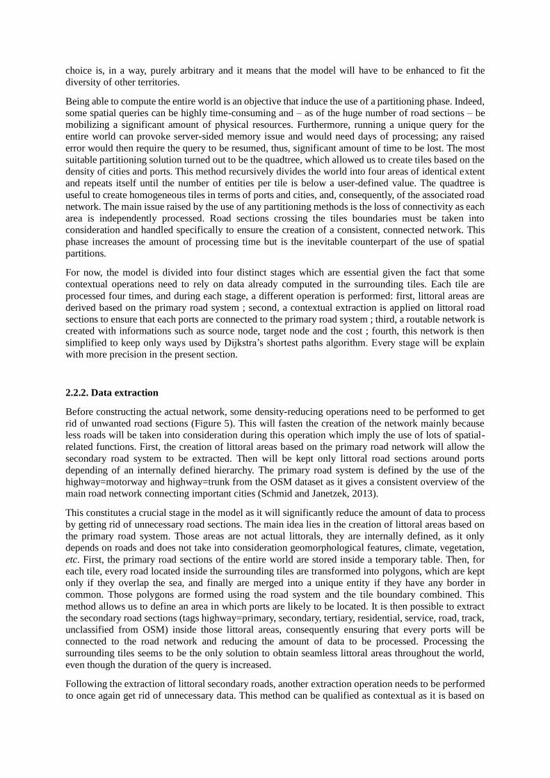
2.2.2. Data extraction
Before constructing the actual network, some density-reducing operations need to be performed to get
rid of unwanted road sections (Figure 5). This will fasten the creation of the network mainly because
less roads will be taken into consideration during this operation which imply the use of lots of spatial-
related functions. First, the creation of littoral areas based on the primary road network will allow the
secondary road system to be extracted. Then will be kept only littoral road sections around ports
depending of an internally defined hierarchy. The primary road system is defined by the use of the
highway=motorway and highway=trunk from the OSM dataset as it gives a consistent overview of the
main road network connecting important cities (Schmid and Janetzek, 2013).
This constitutes a crucial stage in the model as it will significantly reduce the amount of data to process
by getting rid of unnecessary road sections. The main idea lies in the creation of littoral areas based on
the primary road system. Those areas are not actual littorals, they are internally defined, as it only
depends on roads and does not take into consideration geomorphological features, climate, vegetation,
etc. First, the primary road sections of the entire world are stored inside a temporary table. Then, for
each tile, every road located inside the surrounding tiles are transformed into polygons, which are kept
only if they overlap the sea, and finally are merged into a unique entity if they have any border in
common. Those polygons are formed using the road system and the tile boundary combined. This
method allows us to define an area in which ports are likely to be located. It is then possible to extract
the secondary road sections (tags highway=primary, secondary, tertiary, residential, service, road, track,
unclassified from OSM) inside those littoral areas, consequently ensuring that every ports will be
connected to the road network and reducing the amount of data to be processed. Processing the
surrounding tiles seems to be the only solution to obtain seamless littoral areas throughout the world,
even though the duration of the query is increased.
Following the extraction of littoral secondary roads, another extraction operation needs to be performed
to once again get rid of unnecessary data. This method can be qualified as contextual as it is based on
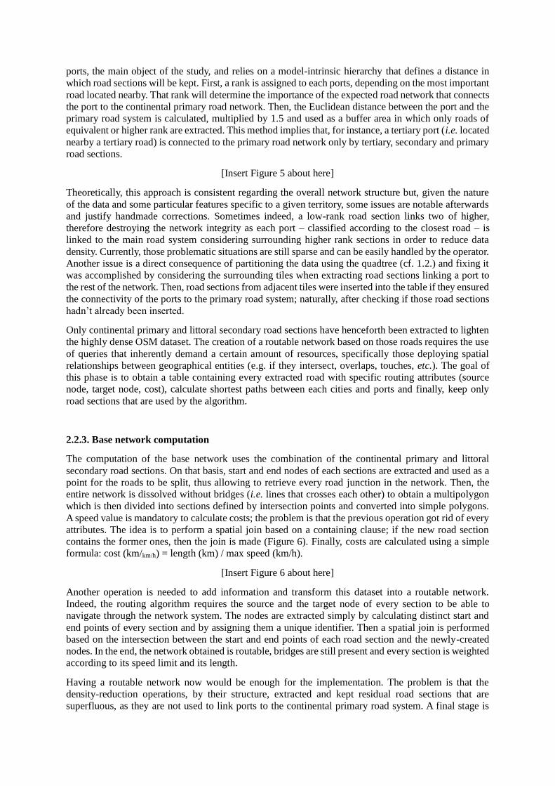
ports, the main object of the study, and relies on a model-intrinsic hierarchy that defines a distance in
which road sections will be kept. First, a rank is assigned to each ports, depending on the most important
road located nearby. That rank will determine the importance of the expected road network that connects
the port to the continental primary road network. Then, the Euclidean distance between the port and the
primary road system is calculated, multiplied by 1.5 and used as a buffer area in which only roads of
equivalent or higher rank are extracted. This method implies that, for instance, a tertiary port (i.e. located
nearby a tertiary road) is connected to the primary road network only by tertiary, secondary and primary
road sections.
[Insert Figure 5 about here]
Theoretically, this approach is consistent regarding the overall network structure but, given the nature
of the data and some particular features specific to a given territory, some issues are notable afterwards
and justify handmade corrections. Sometimes indeed, a low-rank road section links two of higher,
therefore destroying the network integrity as each port – classified according to the closest road – is
linked to the main road system considering surrounding higher rank sections in order to reduce data
density. Currently, those problematic situations are still sparse and can be easily handled by the operator.
Another issue is a direct consequence of partitioning the data using the quadtree (cf. 1.2.) and fixing it
was accomplished by considering the surrounding tiles when extracting road sections linking a port to
the rest of the network. Then, road sections from adjacent tiles were inserted into the table if they ensured
the connectivity of the ports to the primary road system; naturally, after checking if those road sections
hadn’t already been inserted.
Only continental primary and littoral secondary road sections have henceforth been extracted to lighten
the highly dense OSM dataset. The creation of a routable network based on those roads requires the use
of queries that inherently demand a certain amount of resources, specifically those deploying spatial
relationships between geographical entities (e.g. if they intersect, overlaps, touches, etc.). The goal of
this phase is to obtain a table containing every extracted road with specific routing attributes (source
node, target node, cost), calculate shortest paths between each cities and ports and finally, keep only
road sections that are used by the algorithm.
2.2.3. Base network computation
The computation of the base network uses the combination of the continental primary and littoral
secondary road sections. On that basis, start and end nodes of each sections are extracted and used as a
point for the roads to be split, thus allowing to retrieve every road junction in the network. Then, the
entire network is dissolved without bridges (i.e. lines that crosses each other) to obtain a multipolygon
which is then divided into sections defined by intersection points and converted into simple polygons.
A speed value is mandatory to calculate costs; the problem is that the previous operation got rid of every
attributes. The idea is to perform a spatial join based on a containing clause; if the new road section
contains the former ones, then the join is made (Figure 6). Finally, costs are calculated using a simple
formula: cost (km/km/h) = length (km) / max speed (km/h).
[Insert Figure 6 about here]
Another operation is needed to add information and transform this dataset into a routable network.
Indeed, the routing algorithm requires the source and the target node of every section to be able to
navigate through the network system. The nodes are extracted simply by calculating distinct start and
end points of every section and by assigning them a unique identifier. Then a spatial join is performed
based on the intersection between the start and end points of each road section and the newly-created
nodes. In the end, the network obtained is routable, bridges are still present and every section is weighted
according to its speed limit and its length.
Having a routable network now would be enough for the implementation. The problem is that the
density-reduction operations, by their structure, extracted and kept residual road sections that are
superfluous, as they are not used to link ports to the continental primary road system. A final stage is
then essential to eliminate them and guarantee a fully lighten network: calculating the shortest paths
between each main nodes of the network (ports and cities) and keep only necessarily followed road
sections. To achieve this goal, the PostGIS implementation of Dijkstra’s algorithm is deployed and are
extracted only roads sections that are used by the computed shortest paths. Keeping the connectivity
between tiles can be ensured by considering all surrounding tiles during the process. Secondly, the road
sections that have been extracted are clipped according to the tile boundaries so that no overlapping
features will appear in the final table. The network is re-calculated the same way as in 3.1. to dump
intermediary nodes, artifacts of the previous network computation. The only unnecessary nodes kept are
those located onto the tiles boundaries. Finally, source and target attributes of the road sections are
updated according to the new network nodes (Figure 7).
[Insert Figure 7 about here]
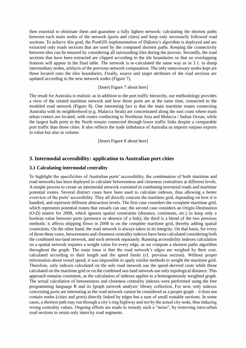
The result for Australia is realistic as in addition to the port traffic hierarchy, our methodology provides
a view of the related maritime network and how those ports are at the same time, connected to the
modeled road network (Figure 8). One interesting fact is that the main maritime routes connecting
Australia with its neighborhood (e.g. Malacca Strait) are concentrated along the east coast where main
urban centers are located, with routes conducting to Northeast Asia and Malacca / Indian Ocean, while
the largest bulk ports in the North remain connected through lower traffic links despite a comparable
port traffic than those cities. It also reflects the trade imbalance of Australia as imports surpass exports
in value but also in volume.
[Insert Figure 8 about here]
3. Intermodal accessibility: application to Australian port cities
3.1 Calculating intermodal centrality
To highlight the specificities of Australian ports’ accessibility, the combination of both maritime and
road networks has been deployed to calculate betweenness and closeness centralities at different levels.
A simple process to create an intermodal network consisted in combining terrestrial roads and maritime
potential routes. Several distinct cases have been used to calculate indexes, thus allowing a better
overview of the ports’ accessibility. They all directly concern the maritime grid, depending on how it is
handled, and represent different abstraction levels. The first case considers the complete maritime grid,
which represents potential routes that vessels can use; the second case considers an Origin-Destination
(O-D) matrix for 2008, which ignores spatial constraints (distance, continents, etc.) to keep only a
boolean value between ports (presence or absence of a link); the third is a blend of the two previous
methods: it affects shipping flows in 2008 to on the complete maritime grid, thereby adding spatial
constraints. On the other hand, the road network is always taken in its integrity. On that basis, for every
of those three cases, betweenness and closeness centrality indexes have been calculated considering both
the combined sea-land network, and each network separately. Running accessibility indexes calculation
on a spatial network requires a weight value for every edge, as we compute a shortest paths algorithm
throughout the graph. The main issue is that the road network’s edges are weighed by their cost,
calculated according to their length and the speed limits (cf. previous section). Without proper
information about vessel speed, it was impossible to apply similar methods to weight the maritime grid.
Therefore, only indexes calculated on the sole road network use the speed-derived costs while those
calculated on the maritime grid or on the combined sea-land network use only topological distance. This
approach remains consistent, as the calculation of indexes applies to a homogeneously weighted graph.
The actual calculation of betweenness and closeness centrality indexes were performed using the free
programming language R and its Igraph network analysis’ library collection. For now, only indexes
concerning ports are interesting as the road network cannot be considered as a proper graph – it does not
contain nodes (cities and ports) directly linked by edges but a sum of small routable sections. In some
cases, a shortest path may run through a city’s ring highway and not by the actual city node, thus inducing
wrong centrality values. Ongoing efforts are made to remedy such a “noise”, by removing intra-urban
road sections to retain only intercity road segments.
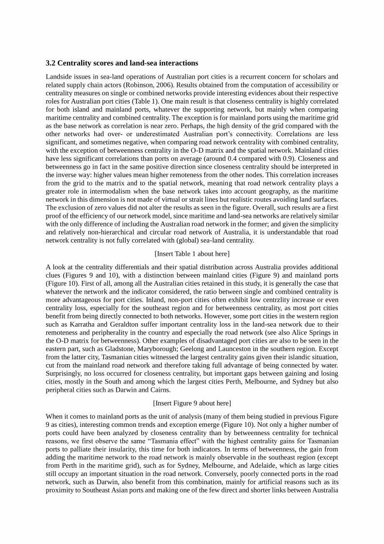
3.2 Centrality scores and land-sea interactions
Landside issues in sea-land operations of Australian port cities is a recurrent concern for scholars and
related supply chain actors (Robinson, 2006). Results obtained from the computation of accessibility or
centrality measures on single or combined networks provide interesting evidences about their respective
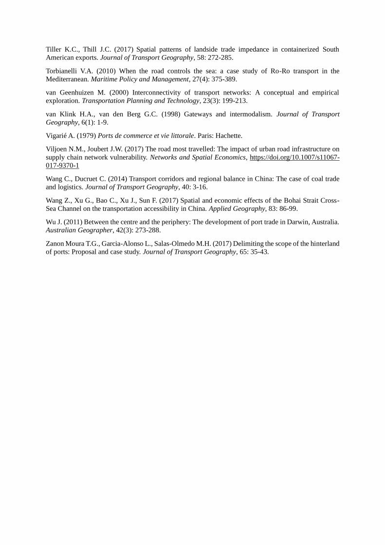
roles for Australian port cities (Table 1). One main result is that closeness centrality is highly correlated
for both island and mainland ports, whatever the supporting network, but mainly when comparing
maritime centrality and combined centrality. The exception is for mainland ports using the maritime grid
as the base network as correlation is near zero. Perhaps, the high density of the grid compared with the
other networks had over- or underestimated Australian port’s connectivity. Correlations are less
significant, and sometimes negative, when comparing road network centrality with combined centrality,
with the exception of betweenness centrality in the O-D matrix and the spatial network. Mainland cities
have less significant correlations than ports on average (around 0.4 compared with 0.9). Closeness and
betweenness go in fact in the same positive direction since closeness centrality should be interpreted in
the inverse way: higher values mean higher remoteness from the other nodes. This correlation increases
from the grid to the matrix and to the spatial network, meaning that road network centrality plays a
greater role in intermodalism when the base network takes into account geography, as the maritime
network in this dimension is not made of virtual or strait lines but realistic routes avoiding land surfaces.
The exclusion of zero values did not alter the results as seen in the figure. Overall, such results are a first
proof of the efficiency of our network model, since maritime and land-sea networks are relatively similar
with the only difference of including the Australian road network in the former; and given the simplicity
and relatively non-hierarchical and circular road network of Australia, it is understandable that road
network centrality is not fully correlated with (global) sea-land centrality.
[Insert Table 1 about here]
A look at the centrality differentials and their spatial distribution across Australia provides additional
clues (Figures 9 and 10), with a distinction between mainland cities (Figure 9) and mainland ports
(Figure 10). First of all, among all the Australian cities retained in this study, it is generally the case that
whatever the network and the indicator considered, the ratio between single and combined centrality is
more advantageous for port cities. Inland, non-port cities often exhibit low centrzlity increase or even
centrality loss, especially for the southeast region and for betweenness centrality, as most port cities
benefit from being directly connected to both networks. However, some port cities in the western region
such as Karratha and Geraldton suffer important centrality loss in the land-sea network due to their
remoteness and peripherality in the country and especially the road network (see also Alice Springs in
the O-D matrix for betweenness). Other examples of disadvantaged port cities are also to be seen in the
eastern part, such as Gladstone, Maryborough; Geelong and Launceston in the southern region. Except
from the latter city, Tasmanian cities witnessed the largest centrality gains given their islandic situation,
cut from the mainland road network and therefore taking full advantage of being connected by water.
Surprisingly, no loss occurred for closeness centrality, but important gaps between gaining and losing
cities, mostly in the South and among which the largest cities Perth, Melbourne, and Sydney but also
peripheral cities such as Darwin and Cairns.
[Insert Figure 9 about here]
When it comes to mainland ports as the unit of analysis (many of them being studied in previous Figure
9 as cities), interesting common trends and exception emerge (Figure 10). Not only a higher number of
ports could have been analyzed by closeness centrality than by betweenness centrality for technical
reasons, we first observe the same “Tasmania effect” with the highest centrality gains for Tasmanian
ports to palliate their insularity, this time for both indicators. In terms of betweenness, the gain from
adding the maritime network to the road network is mainly observable in the southeast region (except
from Perth in the maritime grid), such as for Sydney, Melbourne, and Adelaide, which as large cities
still occupy an important situation in the road network. Conversely, poorly connected ports in the road
network, such as Darwin, also benefit from this combination, mainly for artificial reasons such as its
proximity to Southeast Asian ports and making one of the few direct and shorter links between Australia
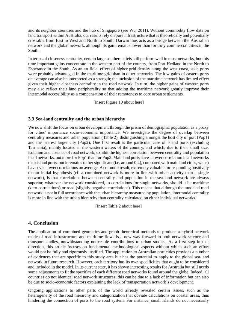
and its neighbor countries and the hub of Singapore (see Wu, 2011). Without commodity flow data on
land transport within Australia, our results rely on pure infrastructure that is theoretically and potentially
crossable from East to West and North to South. Darwin thus acts as a bridge between the Australian
network and the global network, although its gain remains lower than for truly commercial cities in the
South.
In terms of closeness centrality, certain large southern ctieis still perform well in most networks, but this
time important gains concentrate in the western part of the country, from Port Hedland in the North to
Esperance in the South. As an artificial effect of higher grid density along the west coast, such ports
were probably advantaged in the maritime grid than in other networks. The low gains of eastern ports
on average can also be interpreted as a strength; the inclusion of the maritime network has limited effect
given their higher closeness centrality in the road network. In turn, the higher gains of western ports
may also reflect their land peripherality so that adding the maritime network greatly improve their
intermodal accessibility as a compensation of their remoteness to core urban settlements.
[Insert Figure 10 about here]
3.3 Sea-land centrality and the urban hierarchy
We now shift the focus on urban development through the prism of demographic population as a proxy
for cities’ importance socio-economic importance. We investigate the degree of overlap between
centrality measures and urban population (Table 2), distinguishing amongst the host city of port (Pop1)
and the nearest larger city (Pop2). One first result is the particular case of island ports (excluding
Tasmania), mainly located in the western waters of the country, and which, due to their small size,
isolation and absence of road network, exhibit the highest correlation between centrality and population
in all networks, but more for Pop1 than for Pop2. Mainland ports have a lower correlation in all networks
than island ports, but it remains rather significant (i.e. around 0.4), compared with mainland cities, which
have even lower correlations on average. A common result, extremely valuable for responding positively
to our initial hypothesis (cf. a combined network is more in line with urban activity than a single
network), is that correlations between centrality and population in the sea-land network are always
superior, whatever the network considered, to correlations for single networks, should it be maritime
(zero correlations) or road (slightly negative correlations). This means that although the modeled road
network is not in full accordance with the urban hierarchy measured by population, intermodal centrality
is more in line with the urban hierarchy than centrality calculated on either individual networks.
[Insert Table 2 about here]
4. Conclusion
The application of combined geomatics and graph-theoretical methods to produce a hybrid network
made of road infrastructure and maritime flows is a new way forward in both network science and
transport studies, notwithstanding noticeable contributions to urban studies. As a first step in that
direction, this article focuses on fundamental methodological aspects without which such an effort
would not be fully and rigorously justified. The application to Australian port cities provides a number
of evidences that are specific to this study area but has the potential to apply to the global sea-land
network in future research. However, each territory has its own specificities that ought to be considered
and included in the model. In its current state, it has shown interesting results for Australia but still needs
some adjustments to fit the specifics of each different road networks found around the globe. Indeed, all
countries do not identical road network structures; this can be due to a lack of information but can also
be due to socio-economic factors explaining the lack of transportation network’s development.
Ongoing applications to other parts of the world already revealed certain issues, such as the
heterogeneity of the road hierarchy and categorization that obviate calculations on coastal areas, thus
hindering the connection of ports to the road system. For instance, small islands do not necessarily
possess motorways or trunk ways but may have several ports connected by lower-rank roads. Another
issue is the use of different transport modes in countries such as Vietnam or the Democratic Republic of
the Congo. Those two countries have in common to be divided by a large river (i.e. the Mekong and the
Congo), so that the network’s connectivity is maintained through river crossings via ferries to overcome
the lack of bridges along the riverbed.
This feature is being implemented in our model with a proper cost weight to reflect the impact of such
a diversity and to guarantee the presence of terrestrial links between northern and southern Africa.
Lastly, transportation systems are also diverse in terms of their level of network density, from the
sparsely populated Russian steppes to the Japanese megalopolis between Tokyo and Fukuoka. The use
of the quadtree partitioning method seems to prevent inconsistencies linked to the density of population
and transportation infrastructures, but morphologic features such as insularity or, on the contrary, super-
continents such as Afro-Eurasia or the Americas, will inherently bring specific issues. Other
improvements related to purely technical aspects, to enhance both optimization and robustness to obtain
a fast, deployable model everywhere. For example, coastal areas currently take a significant amount of
time to be calculated; this is mainly due to the process of surrounding tiles that, to ensure the
seamlessness of those areas, highly increase the operating time and induce a redundancy that must be
taken care of.
In the end, the model should be working nicely with OpenStreetMap dataset, which contains all the
required features for this kind of network creation (Gil, 2015). But the idea is to create a version that
works as well with other sources such as the Vector Map (VMAP) or any historical data that would
enable studies on the period covered by the informations extracted from the Lloyd’s List corpus. It will
consequently allow us to adapt the model more easily to other road network datasets such as The Vector
Map (or VMAP) for the 1980/90 period. As the mechanics and spatial operations will be the same, those
adjustments shall be quickly implemented, following an equivalent protocol and modifying only minor
features. We also consider weighting the global road network using freely accessible information on the
pavement rate at the country level using Central Intelligence Agency World Factbooks2. Such an
information will allow us to differentiate the score of road network segments depending on the overall
quality and navigability of the transport system.
Overall, this article contributes to a somewhat classical issue in transport economics and geography –
the sea-land interface – while pushing further the technical possibilities of its analysis. It has potential
to deepen our understanding of networks in general, such as a bi-modal or multiplex network being both
planar (road) and non-planar (shipping), which is still rather uncommon in network science. Computing
centrality measures and comparing them with local socio-economic features of the connected nodes will
add crucial evidences to the role of network morphology, connectivity, and complexity in the
understanding of urban and regional development dynamics. Huge efforts are underway to move
towards a more dynamic view of such phenomena, with the extraction of further shipping data and road
network data from older sources. As advised by pioneering scholars in the field (Rimmer, 2015;
Robinson, 2015), the inclusion of other network types such as railways, airlines, and immaterial linkages
(e.g. firms and telecommunications) shall pave the way towards the first-ever analysis of the all-
encompassing network of networks, to further elucidate the role of specialization and diversification
dynamics shaping the evolving world city network. Lastly, another research pathway is the analysis of
the maritime centrality of non-port cities situated inland, thanks to their indirect, landside connection
with the global shipping network. Whenever possible, road traffic data, available from commodity flow
surveys in certain countries, will allow weighting both maritime and landside flows, to complement
existing studies focusing only on the continental area (Duranton et al., 2014).
Acknowledgements
2 https://www.cia.gov/library/publications/the-world-factbook/
The research leading to these results has received funding from the European Research Council under
the European Union's Seventh Framework Programme (FP/2007-2013) / ERC Grant Agreement n.
[313847] "World Seastems".
References
Berroir S., Cattan N., Guérois M., Paulus F., Vacchiani-Marcuzzo C. (2012) Les systèmes urbains
français. Synthèse DATAR, Travaux en Ligne 10.
Bettencourt L.M.A., Lobo J., Helbing D., Künhert C., West G.B. (2007) Growth, innovation, scaling,
and the pace of life in cities. Proceedings of the National Academy of Sciences of the United States of
America, 104(17) : 7301-7306.
Bottasso A., Conti M., de Sa Porto P.C., Ferrari C., Tei A. (2018) Port infrastructures and trade:
Empirical evidence from Brazil. Transportation Research Part A: Policy and Practice, 107: 126-139.
Britton J.N.H. (1965) Coastwise external relations of the ports of Victoria. Australian Geographer, 9(5):
269-281.
Bunel M., Bahoken F., Ducruet C., Lagesse C., Marnot B., Mermet E., Petit S. (2017) Geovisualizing
the sail-to-steam transition through vessel movement data. In: Ducruet C. (Ed.), Advances in Shipping
Data Analysis and Modeling. Tracking and Mapping Maritime Flows in the Age of Big Data. London
and New York: Routledge Studies in Transport Analysis, pp. 189-205.
Catalayud A., Mangan J., Palacin R. (2017) Connectivity to international markets: A multi-layered
network approach. Journal of Transport Geography, 61: 61-71.
Cattan N. (1995) Barrier effects: The case of air and rail flows. International Political Science Review,
16(3): 237-248.
Chapelon L. (2006) L’accessibilité, marqueur des inégalités de rayonnement des villes portuaires en
Europe. Cybergeo: European Journal of Geography, 345: https://cybergeo.revues.org/2463
Choi J.H., Barnett J.A., Chon B.S. (2006) Comparing world city networks: A network analysis of
Internet backbone and air transport intercity linkages. Global Networks, 6(1): 81-99.
Dai L., Derudder B., Liu X. (2017) Generative network models for simulating urban networks, the case
of inter-city transport network in Southeast Asia. Cybergeo: European Journal of Geography, 786:
http://journals.openedition.org/cybergeo/27734
Derudder B., Liu X., Kunaka C., Roberts M. (2014) The connectivity of South Asian cities in
infrastructure networks. Journal of Maps, 10(1): 47-52.
Ducruet (2017) Multilayer dynamics of complex spatial networks: the case of global maritime flows
(1977-2008). Journal of Transport Geography, 60: 47-58.
Ducruet C., Beauguitte L. (2014) Network science and spatial science: Review and outcomes of a
complex relationship. Networks and Spatial Economics, 14(3-4): 297-316.
Ducruet C., Cuyala S., El Hosni A. (2018) Maritime networks as systems of cities: The long-term
interdependencies between global shipping flows and urban development (1890-2010), Journal of
Transport Geography, 66: 340-355.
Ducruet C., Ietri D., Rozenblat C. (2011) Cities in worldwide air and sea flows: A multiple networks
analysis. Cybergeo: European Journal of Geography, 528: http://cybergeo.revues.org/23603
Duranton G., Morrow P., Turner M. (2014) Roads and trade: Evidence from the U.S. Review of
Economic Studies, 81(2): 681-724.
Franc P., Van der Horst M.R. (2010) Analyzing hinterland service integration by shipping lines and
terminal operators in the Hamburg-Le Havre range. Journal of Transport Geography, 18(4): 557-566.
Gil J. (2015) Building a multimodal urban network model using OpenStreetMap data for the analysis of
sustainable accessibility. In: Jokar Arsanjani J., Zipf A., Mooney P., Helbich M. (Eds.), OpenStreetMap
in GIScience: Experiences, Research, Applications, Basel: Springer International Publishing, pp. 229-
251.
Guerrero D., Gonzalez-Laxe F.I., Freire-Seoane M.J., Pais Montes C. (2017) Foreland mix and inland
accessibility of European NUTS-3 regions. In: Ducruet (Ed.), Advances in Shipping Data Analysis and
Modeling. Tracking and Mapping Maritime Flows in the Age of Big Data, London and New York:
Routledge Studies in Transport Analysis, pp. 207-229.
Haklay M. (2010) How good is volunteered geographical information? A comparative study of
OpenStreetMap and Ordnance Survey datasets. Environment and Planning B, 37(4): 682-703.
Halim R.A., Kwakkel J.H., Tavasszy L.A. (2015) The impact of the emergence of direct shipping lines
on port flows. In: Ducruet C. (Ed.), Maritime Networks. Spatial Structures and Time Dynamics, London
and New York: Routledge Studies in Transport Analysis, pp. 265-284.
Halim R.A., Kwakkel J.H., Tavasszy L.A. (2016) A strategic model of port-hinterland freight
distribution networks. Transportation Research Part E: Logistics and Transportation Review, 95: 368-
384.
Hall P.V., Jacobs W. (2012) Why are maritime ports (still) urban, and why should policy makers care?
Maritime Policy and Management, 39(2): 189-206.
Jacobs W., Ducruet C., De Langen P.W. (2010) Integrating world cities into production networks: The
case of port cities. Global Networks, 10(1): 92-113.
Jacobs W., Koster H.R.A., Hall P.V. (2011) The location and global network structure of maritime
advanced producer services. Urban Studies, 48(13): 2749-2769.
Jung P.H., Kashiha M., Thill J.C. (2018) Community structures in networks of disaggregated cargo flows
to maritime ports. In: Popovich V., Schrenk M., Thill J.C., Claramunt C., Wang T. (Eds.), Information
Fusion and Intelligent Geographic Information Systems (IF&IGIS'17), Basel: Springer International
Publishing, pp. 167-186.
Kennedy C.A., Stewart I., Facchini A., Cersosimo I., Mele R., Chen B., Uda M., Kansal A., Chiu A.,
Kim A., Dubeux C., Lebre La Rovere E., Cunha B., Pincetl S., Keirsteadi J., Barles S., Pusakak S.,
Gunawan J., Adegbile M., Nazariha M., Hoque S., Marcotullio P.J., Gonzalez Otharan F., Genena T.,
Ibrahim N., Farooqui R., Cervantes G., Sahin A.D. (2015) Energy and material flows of megacities.
Proceedings of the National Academy of Sciences, 112(19): 5985-5990.
Liu X., Derudder B., Gago Garcia C. (2013) Exploring the co-evolution of the geographies of air
transport aviation and corporate networks. Journal of Transport Geography, 30: 26-36.
Matisziw T.C., Grubesic T.H. (2010) Evaluating locational accessibility to the US air transportation
system. Transportation Research Part A, 44(9): 710-722.
Neal Z. (2017) The urban metabolism of airline passengers: Scaling and sustainability. Urban Studies,
55(1): 212-225.
Nelson A. (2008) Travel time to major cities: A global map of accessibility. Global Environment
Monitoring Unit, Joint Research Centre of the European Commission, Ispra, Italy.
Ng A.K.Y., Ducruet C., Jacobs W., Monios J., Notteboom T.E., Rodrigue J.P., Slack B., Tam K.C.,
Wilmsmeier G. (2014) Port geography at the crossroads with human geography: Between flows and
spaces. Journal of Transport Geography, 41: 84-96.
Notteboom T.E., Parola F., Satta G., Pallis A.A. (2017) The relationship between port choice and
terminal involvement of alliance members in container shipping. Journal of Transport Geography, 64:
168-173.
O’Connor K. (1989) Australian ports, metropolitan areas and trade-related services. Australian
Geographer, 20(2): 167-172.
Observatory of Economic Complexity (2018) Australia.
https://atlas.media.mit.edu/en/profile/country/aus/
Paflioti P., Vitsounis T.K., Teye C., Bell M.G.H., Tsamourgelis I. (2017) Box dynamics: A sectoral
approach to analyse containerized port throughput interdependencies. Transportation Research Part A:
Policy and Practice, 106: 396-413.
Peris A. (2016) Penser les villes en réseaux : une analyse des théories sur les liens interurbains. Master
Dissertation in Geography, University of Paris I Panthéon-Sorbonne.
Qu Y., Bektas T., Bennell J. (2016) Sustainability SI: Multimode multicommodity network design model
for intermodal freight transportation with transfer and emission costs. Networks and Spatial Economics,
16(1): 303-329.
Rimmer P.J. (1967) The search for spatial regularities in the development of Australian seaports 1861–
1961/2. Geografiska Annaler B, 49(1): 42-54.
Rimmer P.J. (2015) Foreword. In: Ducruet C. (dir.) Maritime Networks. Spatial Structures and Time
Dynamics, London and New York: Routledge, pp. xxi-xxiii.
Robinson R. (2006) Port-oriented landside logistics in Australian ports: A strategic framework.
Maritime Economics and Logistics, 8(1): 40-59.
Robinson R. (2007) Regulating efficiency into port-oriented chain systems: export coal through the
Dalrymple Bay Terminal, Australia. Maritime Policy and Management, 34(2): 89-106.
Robinson R. (2015a) Afterword. In: Ducruet C. (Ed.), Maritime Networks. Spatial Structures and Time
Dynamics, London and New York: Routledge Studies in Transport Analysis, pp. 374-377.
Robinson R. (2015b) Cooperation strategies in port-oriented bulk supply chains: aligning concept and
practice. International Journal of Logistics Research and Applications, 18(3): 193-206.
Rosato V., Issacharoff L., Tiriticco F., Meloni S., De Porcellinis S., Setola R. (2008) Modelling
interdependent infrastructures using interacting dynamical models. International Journal of Critical
Infrastructures, 4(1-2): 63-79.
Roso V., Woxenius J., Lumsden K. (2009) The dry port concept: Connecting container seaports with the
hinterland. Journal of Transport Geography, 17(5): 338-345.
Schmid F., Janetzek H. (2013) A Method for High-Level Street Network Extraction of OpenStreetMap
Data in OpenScienceMap. International Cartographic Conference, 92:
http://icaci.org/files/documents/ICC_proceedings/ICC2013/_extendedAbstract/92_proceeding.pdf
Shen G. (2017) GIS-based analysis of US international seaborne trade flows. In: Ducruet (Ed.),
Advances in Shipping Data Analysis and Modeling. Tracking and Mapping Maritime Flows in the Age
of Big Data, London and New York: Routledge Studies in Transport Analysis, pp. 147-172.
Slack B. (2017) Epilogue. In: Ducruet (Ed.), Advances in Shipping Data Analysis and Modeling.
Tracking and Mapping Maritime Flows in the Age of Big Data, London and New York: Routledge
Studies in Transport Analysis, pp. 437-440.
Taylor P.J., Derudder B. (2016) World City Network. A global Urban Analysis, 2nd Edition, London and
New York: Routledge.
Tiller K.C., Thill J.C. (2017) Spatial patterns of landside trade impedance in containerized South
American exports. Journal of Transport Geography, 58: 272-285.
Torbianelli V.A. (2010) When the road controls the sea: a case study of Ro-Ro transport in the
Mediterranean. Maritime Policy and Management, 27(4): 375-389.
van Geenhuizen M. (2000) Interconnectivity of transport networks: A conceptual and empirical
exploration. Transportation Planning and Technology, 23(3): 199-213.
van Klink H.A., van den Berg G.C. (1998) Gateways and intermodalism. Journal of Transport
Geography, 6(1): 1-9.
Vigarié A. (1979) Ports de commerce et vie littorale. Paris: Hachette.
Viljoen N.M., Joubert J.W. (2017) The road most travelled: The impact of urban road infrastructure on
supply chain network vulnerability. Networks and Spatial Economics, https://doi.org/10.1007/s11067-
017-9370-1
Wang C., Ducruet C. (2014) Transport corridors and regional balance in China: The case of coal trade
and logistics. Journal of Transport Geography, 40: 3-16.
Wang Z., Xu G., Bao C., Xu J., Sun F. (2017) Spatial and economic effects of the Bohai Strait Cross-
Sea Channel on the transportation accessibility in China. Applied Geography, 83: 86-99.
Wu J. (2011) Between the centre and the periphery: The development of port trade in Darwin, Australia.
Australian Geographer, 42(3): 273-288.
Zanon Moura T.G., Garcia-Alonso L., Salas-Olmedo M.H. (2017) Delimiting the scope of the hinterland
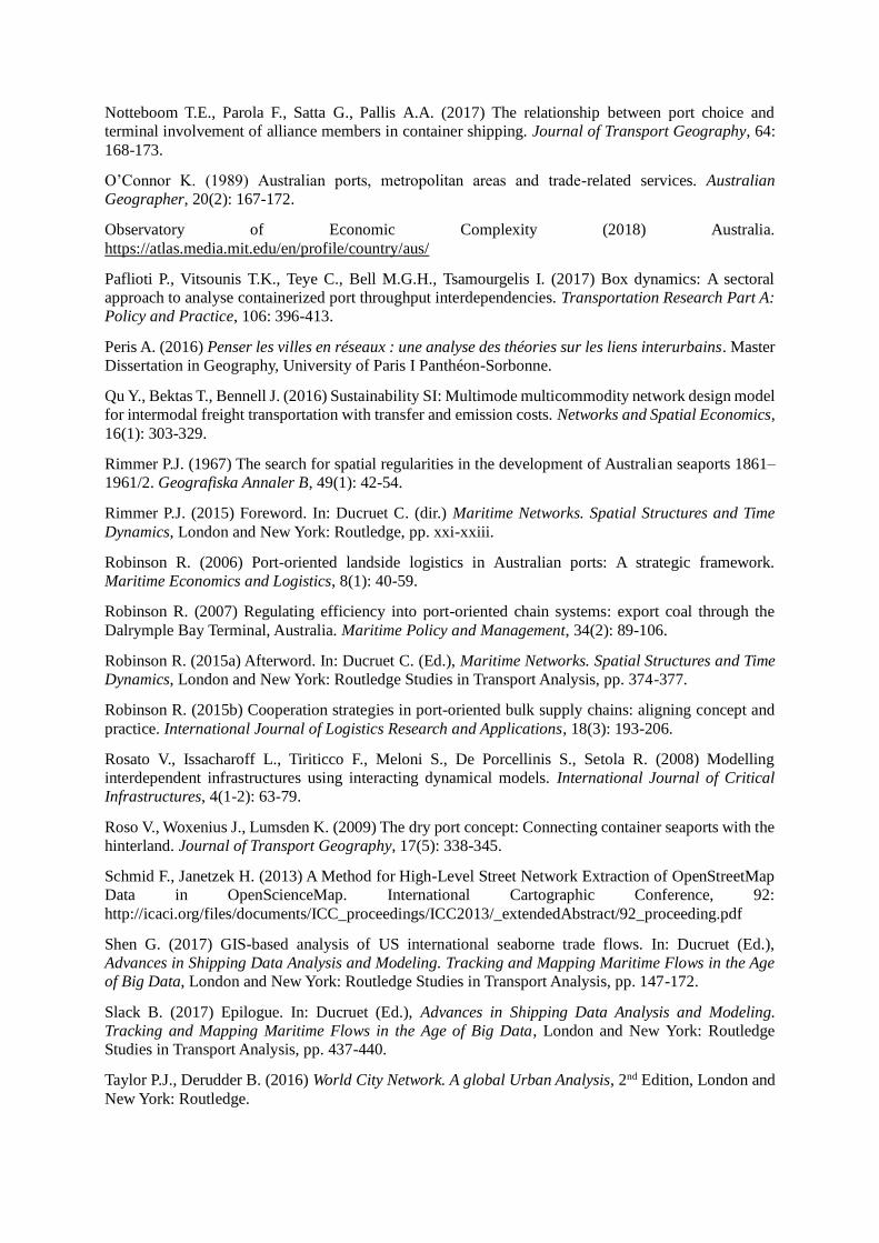
of ports: Proposal and case study. Journal of Transport Geography, 65: 35-43.
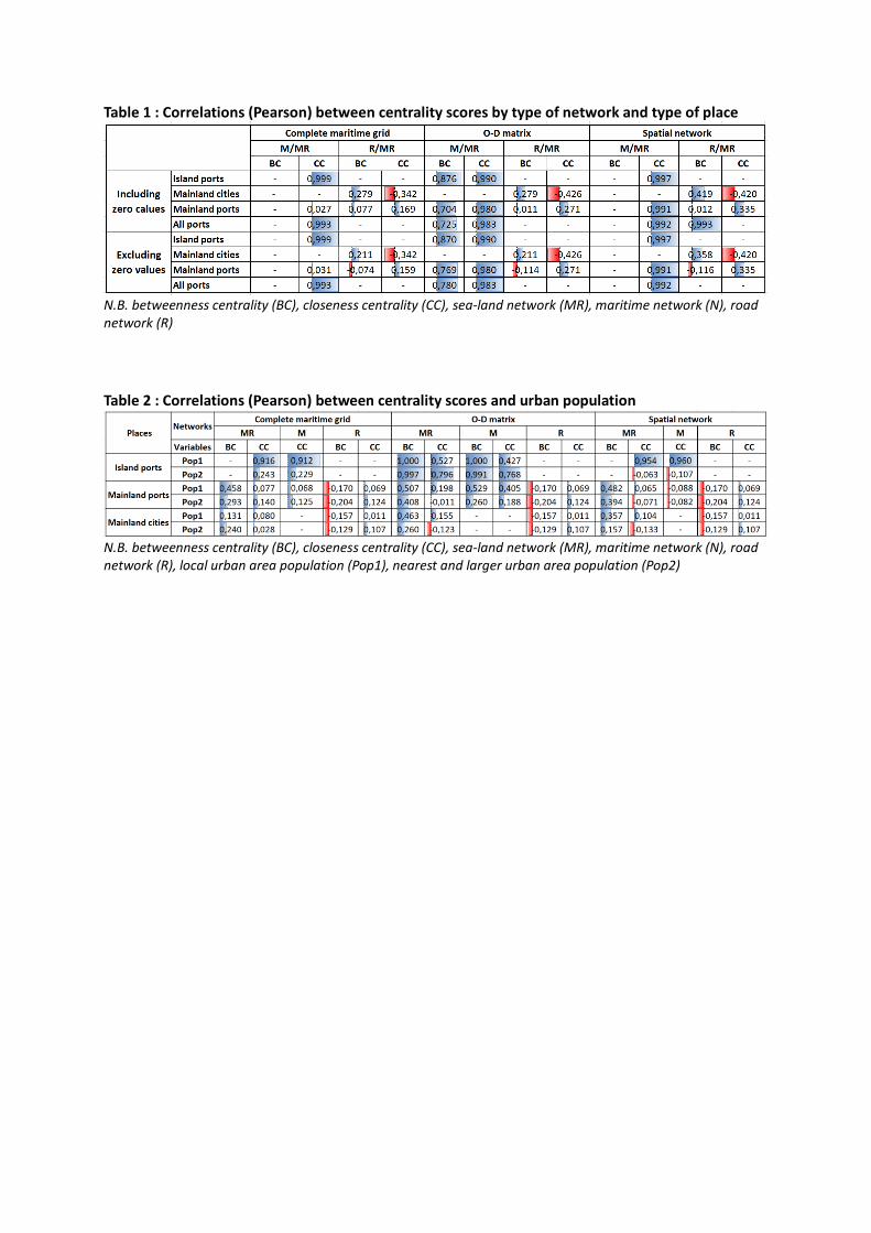
Table 1 : Correlations (Pearson) between centrality scores by type of network and type of place
N.B. betweenness centrality (BC), closeness centrality (CC), sea-land network (MR), maritime network (N), road network (R)
Table 2 : Correlations (Pearson) between centrality scores and urban population
N.B. betweenness centrality (BC), closeness centrality (CC), sea-land network (MR), maritime network (N), road network (R), local urban area population (Pop1), nearest and larger urban area population (Pop2)
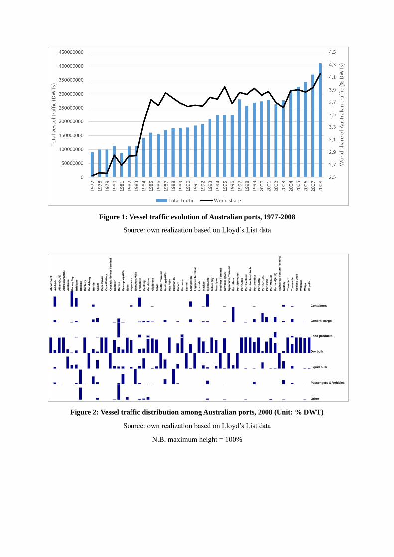
Figure 1: Vessel traffic evolution of Australian ports, 1977-2008
Source: own realization based on Lloyd’s List data
Figure 2: Vessel traffic distribution among Australian ports, 2008 (Unit: % DWT)
Source: own realization based on Lloyd’s List data
N.B. maximum height = 100%
Containers
General cargo
Food products
Dry bulk
Liquid bulk
Passengers & Vehicles
Other
Ab
bo
t P
oin
t
Ad
ela
ide
Alb
an
y(A
US
)
Ard
rossan
(AU
S)
Au
str
ali
a
Bo
tan
y B
ay
Bri
sb
an
e
Bro
om
e
Bu
nb
ury
Bu
nd
ab
erg
Bu
rnie
Cair
ns
Cap
e C
uvie
r
Cap
e F
latt
ery
Co
ssack P
ion
eer
Term
inal
Dam
pie
r
Darw
in
Devo
np
ort
(AU
S)
Ed
en
Esp
era
nce
Exm
ou
th(A
US
)
Fre
man
tle
Geelo
ng
Gera
ldto
n
Gla
dsto
ne
Go
ve
Gri
ffin
Term
inal
Hasti
ng
s(A
US
)
Hay P
oin
t
Haym
an
Is.
Ho
bart
Karu
mb
a
Ku
rnell
Lau
ncesto
n
Leg
en
dre
Term
inal
Lu
cin
da
Mackay
Melb
ou
rne
Mil
ner
Bay
Mo
uri
lyan
Mu
tin
eer
Term
inal
New
castl
e(A
US
)
Ng
an
hu
rra T
erm
inal
Po
rt A
lma
Po
rt B
on
yth
on
Po
rt G
iles
Po
rt H
ed
lan
d
Po
rt H
ed
lan
d A
nch
.
Po
rt K
em
bla
Po
rt L
att
a
Po
rt L
inco
ln
Po
rt P
irie
Po
rt W
alc
ott
Po
rtla
nd
(AU
S)
Sty
barr
ow
Ven
ture
Term
inal
Syd
ney
Th
even
ard
To
wn
svil
le
Usele
ss L
oo
p
Wall
aro
o
Weip
a
Wh
yall
a
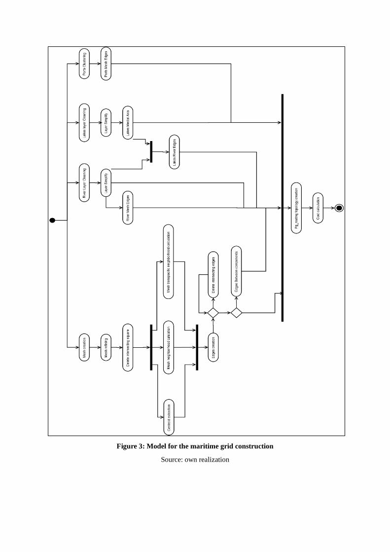
Figure 3: Model for the maritime grid construction
Source: own realization
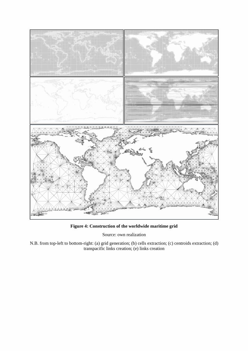
Figure 4: Construction of the worldwide maritime grid
Source: own realization
N.B. from top-left to bottom-right: (a) grid generation; (b) cells extraction; (c) centroids extraction; (d)
transpacific links creation; (e) links creation
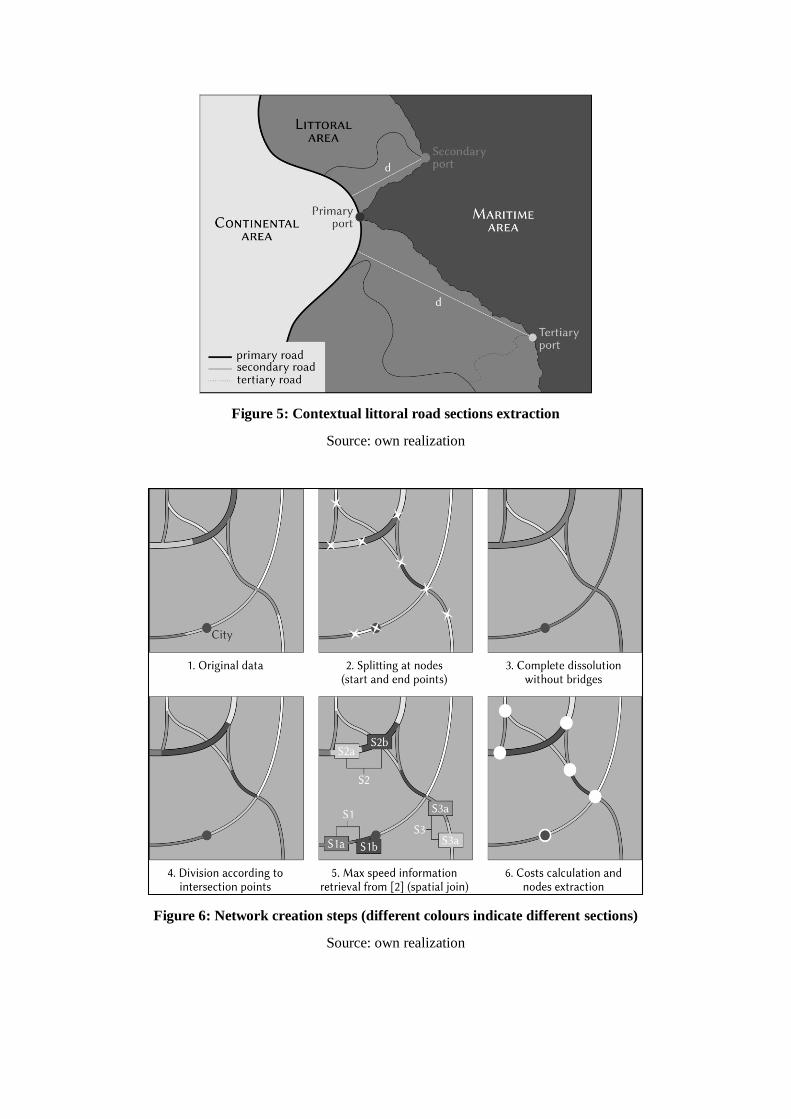
Figure 5: Contextual littoral road sections extraction
Source: own realization
Figure 6: Network creation steps (different colours indicate different sections)
Source: own realization
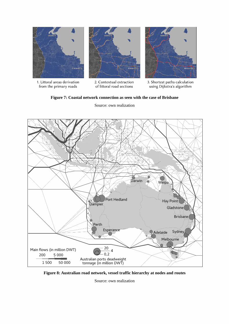
Figure 7: Coastal network connection as seen with the case of Brisbane
Source: own realization
Figure 8: Australian road network, vessel traffic hierarchy at nodes and routes
Source: own realization
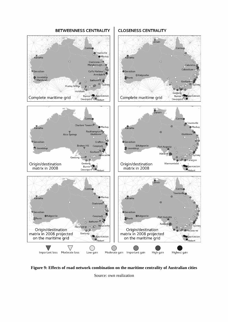
Figure 9: Effects of road network combination on the maritime centrality of Australian cities
Source: own realization
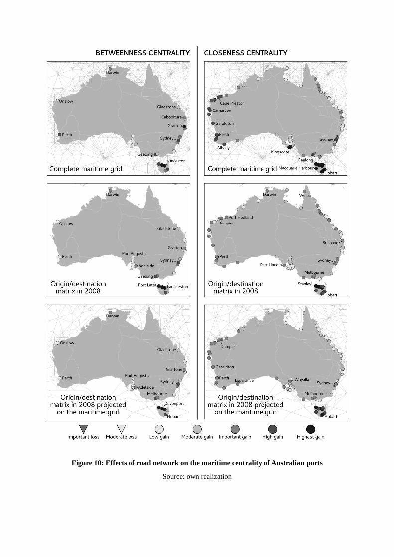
Figure 10: Effects of road network on the maritime centrality of Australian ports
Source: own realization