Q.No.1: Assume that you have been contacted by an Organization to developed CAD Software, after applying the size-oriented metrics an estimate of 33200 LOC is established. Using COCOMO model develop an effort, duration and no-of-person for CAD software. Consider the

ab = 2.4, bb = 1.05, cb = 2.5, db = 0.35

Given:LOC = 33200 = 33.2 k

FOR CAD SOFTWARE :

(ab = 2.4, bb = 1.05, cb = 2.5, db = 0.35)

FORMULA:

E = ab (KLOC)^ bb

D = cb (E)^ db

No. of person = E/D

SOLUTION:

E = 2.4 (33.2) ^ 1.05 = 94.93 person months

D = 2.5 (94.93) ^ 0.35 = 12.30 months

No. of persons = 94.93 = 7.7 = 8 persons 12.30

Q.No.2 Explain with examples the LOC-based, FP-based and Process-based Estimation?

Problem-Based Estimation:

LOC and FP estimation are distinct estimation techniques. Yet both have a number of characteristics in common. The project planner begins with a bounded statement of software scope and from this statement attempts to decompose software into problem functions that can each be estimated individually. LOC or FP (the estimation variable) is then estimated for each function.

The LOC and FP estimation techniques differ in the level of detail required for decomposition and the target of the partitioning. When LOC is used as the estimation variable, decomposition is absolutely essential and is often taken to considerable levels of detail.

This decomposition approach assumes that all functions can be decomposed into sub functions that will resemble entries in a historical data base. If this is not the case, then another sizing approach must be applied. The greater the degree of partitioning, the more like reasonable accurate estimates of Loc can be developed.

For FP estimates, decomposition works differently. Rather than focusing on function, each of the information domain characteristics – inputs, outputs, data files, inquiries, and external interfaces. The resultant estimates can then be used to derive a FP value that can be tied to past data and used to generate an estimate.

An Example of LOC-Based Estimation:

Let us consider a software package to be developed for a computer-aided design application for mechanical components. A review of the System Specification indicates that the software is to execute on an engineering workstation and must interface with various computer graphics peripherals including a mouse, digitizer, high resolution color display and laser printer.

Using the System Specification as a guide, a preliminary statement of software scope can be developed:

The CAD software will accept two- and three-dimensional geometric data from an engineer. The engineer will interact and control the CAD system through a user interface that will exhibit characteristics of good human / machine interface design. All geometric data and other supporting information will be maintained in a CAD database. Design analysis modules will be developed to produce the required output, which will be displayed on a variety of graphics devices. The software will be designed to control and interact with peripheral devices that include a mouse, digitizer, laser printer, and plotter.

This statement of scope is preliminary – it is not bounded. Every sentence would have to be expanded to provide concrete detail and quantitative bounding. For example, before estimation can begin the planner must determine what “characteristic of good human / machine interface design. All geometric data and other supporting information will be maintained in a CAD database. Design analysis modules will be developed to produce the required output, which will be displayed on a variety of graphics devices. The software will be designed to control and interact with peripheral devices that include a mouse, digitizer, laser printer, and plotter.

This statement of scope is preliminary – it is not bounded. Every sentence would have to be expanded to provide concrete detail and quantitative bounding. For example, before estimation can being the planner must determine what “characteristics of good human / machine interface deface design” means or what the size and sophistication of the “CAD database” is to be.

For our purposes, we assume that further refinement has occurred and that the following major software functions are identified:

User interface and control facilities (UICF)Two-dimensional geometric analysis (2DGA) Three-dimensional geometric analysis (3DGA)Database management (DBM)Computer graphics display facilities (CGDF)Peripheral control function (PCF)Design analysis modules (DAM)

Following the decomposition technique of LOC, an estimation table, shown in Figure-1, is developed. A range of LOC estimates is developed for each function. For example, the range of LOC estimates for the 3D geometric analysis function is optimistic – 4600 LOC, most likely – 6900 Loc, and pessimistic – 8600 LOC.

Function Estimated LOC

Use interface and control (UICF) 2,300

Two-dimensional geometric analysis (2DGA) 5,300

Three-dimensional geometric analysis (3DGA) 6,800

Database management (DBM) 3,350

Computer graphics display facilities (CGDF) 4,950

Peripheral control function (PCF) 2,100

Design analysis modules (DAM) 8,400

ESTIMATED LINES OF CODE 33,200Figure-1

Applying Equation [S= (Sopt +4Sm+Spe)/6], the expected value for the 3D geometric analysis function is 680 LOC. Other estimates are derived in a similar fashion. By summing vertically in the estimated LOC column, an estimate of 33,200 lines of code is established for the CAD system.

A review of historical data indicates that the organizational average productivity for systems of this type is 620 LOC/pm. Based on a burdened labor rate of $8000 per month; the cost per line of code is approximately $13. Based on the LOC estimate and the historical productivity data, the total estimated project cost is $431,000 and the estimated effort is 54 person-months.

An Example of FP-based estimation:

Decomposition for FP-based estimation focuses on information domain values rather than software functions. Referring to the function point calculation table presented in Figure-2, the project planner estimates inputs, outputs, inquiries, files, and external interfaces for the CAD software. For the purposes of this estimate, the complexity weighting factor is assumed to be average. Figure-2 presents the results of this estimate.

Information domain value Opt. Likely Pess. Est. count Weight FP

countNumber of inputs 20 24 30 24 4 97

Number of outputs 12 15 22 16 5 78

Number of inquiries 16 22 28 22 5 88

Number of files 4 4 5 4 10 42

Number of external interfaces 2 2 3 2 7 15

Count total 320Figure-2

Each of the complexity weighting factors is estimated and the complexity adjustment factor is computed.

Factor Value

Backup and recovery 4

Data communications 2

Distributed processing 0

Performance critical 4

Existing operating environment 3

On-line data entry 4

Input transaction over multiple screens 5

Master files updated on-line 3

Information domain values complex 5

Internal processing complex 5

Code designed for reuse 4

Conversion/installation in design 3

Multiple installations 5

Application designed for change 5

Complexity adjustment factor 1.17

Finally, the estimated number of FP is derived:

FP estimated = count-total x [0.65 + 0.01 x (Fj)]FP estimated = 375

The organizational average productivity for systems of this type is 6.5FP/pm. Based on a burdened labor rate of $8000 per month, the cost per FP is approximately $1230. Based on the LOC estimate and the historical productivity data, the total estimated project cost is $461,000 and the estimated effort is 58 person-months.

Process-Based Estimation:

The most common technique for estimating a project is to base the estimate on the process that will be used. That is, the process is decomposed into a relatively small set of tasks and the effort required to accomplish each task is estimated.

Like the problem-based techniques, process-based estimation begins with a delineation of software functions obtained from the project scope. A series of software process activities must be performed for each function.

Once problem functions and process activities are melded, the planner estimates the effort (e.g., person-months) that will be required to accomplish each software process activities for each software function.

Activity CC Planning Risk analysis

Engineering Construction release

CE Totals

Task Analysis Design Code Test

Function UICF 0.50 2.50 0.40 5.00 n/a 8.402DGA 0.75 4.00 0.60 2.00 n/a 7.353DGA 0.50 4.00 1.00 3.00 n/a 8.50CGDF 0.50 3.00 1.00 1.50 n/a 6.00DBM 0.50 3.00 0.75 1.50 n/a 5.75PCF 0.25 2.00 0.50 1.50 n/a 4.25DAM 0.50 2.00 0.50 2.00 n/a 5.00

Total 0.25 0.25 0.25 3.50 20.50 4.50 16.50 46.00

% effort 1% 1% 1% 8% 45% 10% 36%Figure-3

CC = customer communication CE = customer evaluation

Costs and effort for each function and software process activity are computed as the last step.

An Example of Process-Based Estimation:

To illustrate the use of process-based estimation, we consider the CAD software. The system configuration and all software functions remain unchanged and are indicated by project scope.

Referring to the completed process-based table shown in Figure-3, estimates of effort (in person-months) for each software engineering activity are provided for each Cad software function (abbreviated for brevity). The engineering and construction release activities are subdivided into the major software engineering tasks shown. Gross estimates of effort are provided for customer communication, planning, and risk analysis. These are noted in the total row at eh bottom of the table. Horizontal and vertical totals provide and indication of estimated effort required for analysis, design, code, and test. It should be noted that 53 percent of all effort is expended on front-end engineering tasks (requirements analysis and design), indicating the relative importance of this work.

Based on an average burdened labor rate of $8000 per month, the total estimated project cost is $368000 and the estimated effort is 46 person-months. If desired, labor rates could be associated with each software process activity or software engineering task and computed separately.

Total estimated effort for the CAD software range from a low of 465 person-months 9derived using a process-based estimation approach) to a high of 58 person-months (derived using an FP estimation approach). The average estimate (using all three approaches) is 53 person-months. The maximum variation from the average estimate is approximately 13 percent.

Q.No 3(a) Explain Software Size and function oriented matrices and Measurements?

Measurement:

Measurements in the physical world can be categorized in two ways: direct measures (e.g., the length of bolt) and indirect measures (e.g., the “quality” of bolt produced, measured by counting rejects). Software metrics can be categorized similarly.

Direct measures of the software engineering process include cost and effort applied. Direct measures of the product include lines of code (LOC) produced, execution speed, memory size, and defects reported over some set period of time. Indirect measures of the product include functionality, quality, complexity, efficiency, reliability, maintainability, and many other “-abilities”.

The cost and effort required building software, the number of lines of code produced, and other direct measures are relatively easy to collect, as long as specific conventions for measurement are established in advance. However, the quality and functionality of software or its efficiency or maintainability are more difficult to assess and can be measured only indirectly.

Size-Oriented Metrics:

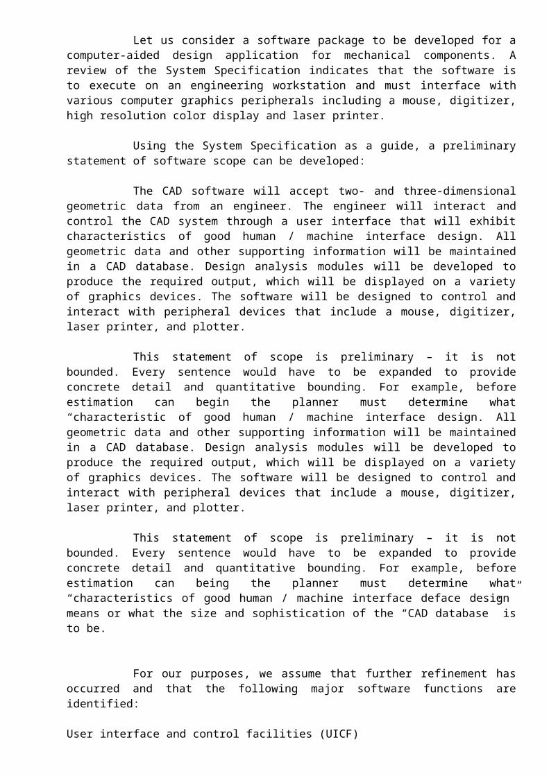
Size-oriented software metrics are derived by normalizing quality and / or productivity measures by considering the size of the software that has been produced. If a software organization maintains simple records, a table of size-oriented measures such as the one show in Figure 4.4, can be created. The table lists each software development project that has been completed over the past few years and corresponding measures for the project. Referring to the table entry for project alpha: 12,100 lines of code were developed with 24 person-months of effort at a cost of $168,000. It should be noted that the effort and cost recorded in the table represent all software engineering activities (analysis, design, code, and test), not just coding. Further information for project alpha indicates that 365 pages of documentation were developed, 134 errors were recorded before the software was released, and 29 defects were encountered after release to the customer within the first year of operation. Three people worked on the development of software for project alpha.

Project LOC Effort $ (000) Pp. doc. Errors Defects PeopleAlpha 12100 24 168 365 134 29 3Beta 27200 62 440 1224 321 86 5Gamma 20200 43 314 1050 256 64 6- - - - - - - -- - - - - - - -- - - - - - - -

If we chose lines of code as our normalization value. From the rudimentary data contained in the table, a set of simple size-oriented metrics can be developed for each project:Errors per KLOC (thousand lines of code).Defects 4 per KLOC. $ Per LOC.Page of documentation per KLOC.

In addition, other interesting metrics can be computed:Errors per person-month.LOC per person-month.$ Per page of documentation.

Function-Oriented Metrics:

Function-oriented software metrics use a measure of the functionality delivered by the application as a normalization value. Since ‘functionality’ cannot be measured directly, it must be derived indirectly using other direct measures. Function-oriented metrics were first proposed by Albrecht, who suggested a measure called the function point. Function points are derived using an empirical relationship based on countable (direct) measures of software’s information domain and assessments of software complexity.

Function points are computed by completing the table shown in Figure-4. Five information domain characteristics are determined and counts are provided in the appropriate table location. Information domain values are defined in the following manner.

Weighting factorMeasurement Parameter Count Simple Average Complex

Number of user inputs x 3 4 6 =

Number of user outputs x 4 5 7 =

Number of user inquiries x 3 4 6 =

Number of files x 7 10 15 =

Number of external interfaces x 5 7 10 =

Count total

Figure-4

Number of user inputsNumber of user outputsNumber of user inquiriesNumber of filesNumber of external interfaces.

To compute function points (FP), the following relationship is used:FP = count total x [0.65 + 0.01 x (Fi)]Where count total is the sum of all FP entries obtained from Figure-4.The Fi (i = 1 to 14) are “complexity adjustment values”.

Once Function points have been calculated, they are used in a manner analogous to LOC as a way to normalize measures for software productivity, quality, and other attributes:

Errors per FP.Defects per FP. $ per FPPages of documentation per FP. FP per person-month.

Q.3 No (b) Established a goal –driven software program?

Establishing a Software Metrics Program:

The Software Engineering Institute has developed a comprehensive guidebook for establishing a “goal-driven” software metrics program. The guidebook suggests the following steps:

Identify you business goals.Identify what you want to know or learnIdentify your sub goals. Identify the entities and attributes related to your sub goals. Formalize your measurement goals. Identify quantifiable questions and the related indicators that you will use to help you achieve your measurement goals. Identify the data elements that you will collect to construct the indicators that help answer your questions.Define the measures to be used, and make these definitions operations. Identify the actions that you will take to implement the measures. Prepared a plan for implementing the measures.

A detailed discussion of these steps is best left to the SEI’s guidebook. However, a brief overview of key points is worthwhile.

Because software supports business functions, differentiates computer-based system to products, or acts as a product in itself, goals defined for the business can almost always be traced downward to specific goals at the software engineering level. For example, consider a company that makes advanced home security systems which have substantial software content. Working as a team, software engineering and business managers can develop a list of prioritized business goals:

Improve our customers’ satisfaction with out products. Make our products easier to use. Reduce the time it takes us to get a new product to market. Make support for our products easier. Improve our overall profitability.

The software organization examines each business goal and asks: “What activities do we manage or execute and what do we want to improve within these activities?” To answer these questions the SEI recommends the creation of an “entity-question list” in which all things (entities) within the software process that are managed or influenced by the software organization are noted. Examples of entities include development resources, work products, source code, test cases, change requests, software engineering tasks, and schedule. For each entity listed, software people develop a set of questions that assess quantitative characteristics of the entity (e.g. size, cost, time to develop). The questions derived as a consequence of the creation of an entity-question list lead to the derivation of a set of sub goals that relate directly to the entities created and the activities performed as part of the software process.

Consider the fourth goal: “Make support for our products easier.” The following list of questions might be derived for this goal:

Do customer change requests contain the information we require to adequately evaluate the change and then implement it in a timely manner?How large is the change request backlog?Is our response time for fixing bugs acceptable based on customer need?Is our change control process followed?Are high-priority changes implemented in a timely manner?

Based on these questions, the software organization can derive the following sub goal: improve the performance of the change management process. The software process entities and attributes that are relevant to the sub goal are identified and measurement goals associated with them are delineated.

The SEI provides detailed guidance for steps 6 through 10 of its goal-driven measurement approach. In essence, a process of stepwise refinement is applied in which goals are refined into questions that are further refined into entities and attributes that are then refined into metrics.

Q No.04.Compute 3D function point value for an embedded system with following characteristics.

-Internal data structures = 6, -External data structures = 3, -No. of user inputs = 12, -No. of user outputs = 60, -No. of user enquiries = 9, -Transformation = 36, -Transition = 24, Assuming the complexity of the above counts is average. Solution:

First we’ll compute function points

Measurement Parameter Count Weight Functional CountNo: of user inputs 12 4 36No: of user outputs 60 5 300No: of user enquiries 9 4 36Internal data structures 6 10 60External data structures 3 7 21Transformations 36 5 180Transitions 24 - 24Count Total 657

Now assume that 14 questions have been counted and are equal to To 14) = 42

FP = Count Total * [0.65 + 0.01 * ] = 657 * [0.65+0.01*42] = 703 approx.

Q.No 5 Write Short Notes?

(a) Adaptation Criteria:

Adaptation criteria are used to determine the recommended degree of rigor with which the software process should be applied on a project. Eleven adaptation criteria [PRE99] are defined for software projects:

Size of the projectNumber of potential usersMission CriticalityApplication longevity Stability of requirementsEase of customer / developer communicationMaturity of applicable technology Performance ConstraintsEmbedded and non embedded characteristicsProject staffReengineering factors

Each of the adaptation criteria is assigned a grade that ranges between 1 and 5, where 1 represents a project win which a small subset of process tasks are required and overall methodological and documentation requirements are minimal, and 5 represents a project in which a complete set of process tasks should be applied and overall methodological and documentation requirements are substantial.

(b) Earned Value Analysis:

A technique for performing quantitative analysis of progress does exist. It is called earned value analysis (EVA).

Humphrey (HUM95) discusses earned value in the following manner:

The earned value system provides a common value scale for every [software project] task, regardless of the type of work being performed. The total hours to do the whole project are estimated, and ever task is given an earned value based on its estimated percentage of the total.

Stated even more simply, earned value is a measure of progress. It enables us to assess the “percent of completeness” off a project using quantitative analysis rather than rely on a gut feeling. In fact, Fleming and Koppleman [FLE98] argue that earned value analysis “provides accurate and reliable readings of performance from as early as 15 percent into the project.”

The budgeted cost of work scheduled (BCWS) determined for each work task represented in the schedule. During the estimation activity, the work (in person-hours or person-days) of each of each software engineering task is planned. Hence, BCWS, is the effort planned for work task i. To determine progress at a given point along the project schedule, the value of BCWS is the sum of the BCWS, value for all work tasks that should have been completed by that point in time on the project schedule.

The BCWS values for all works tasks are summed to derive the budget at completion, BAC. Hence,

BAC = (BCWSK) for all tasks kNext, the value for budgeted cost of work performed (BCWP) is computed. The value of BCWP is the sum of the BCWS values for all work tasks that have actually been completed by a point in time on the project schedule.

Given values for BCWS, BAC, and BCWP, important progress indicators can be computed:

Schedule performance index, SPI = BCWP / BCWSSchedule variance, SV = BCWP – BCWS

SPI is an indication of the efficiency with which the project is utilizing scheduled resources. An SPI value close to 1.0 indicates efficient execution of the project schedule. SV is simply an absolute indication of variance from the planned schedule.

(c) Outsourcing:

In concept, outsourcing is extremely simple. Software engineering activities are contacted to a third party who does the work at lower cost and, hopefully, higher quality. Software work conducted within a company is reduced to a contract management activity.

The decision to outsource can be either strategic or tactical. At the strategic level, business managers consider whether a significant portion of all software work can be contracted to others. At the tactical level, a project manager determines whether part or all of a project can be best accomplished by subcontracting the software work.

Regardless of the breadth of focus, the outsourcing decision is often a financial one.

On the positive side, cost savings can usually be achieved by reducing the number of software people and the facilities (e.g., computers, infrastructure) that support them. On the negative side, a company loses some control over the software that it needs. Since software is a technology that differentiates its systems, services, and products, a company runs the risk of putting the fate of its competitiveness into the hands of a third party.

The trend toward outsourcing will undoubtedly continue. The only way to blunt the trend is to recognize that software work is extremely competitive at all levels. The only way to survive is to become as competitive as the outsourcing vendors themselves.

(d) CASE (Computer-Aided Software Engineering):

Computer–aided software engineering (CASE) tools assist software engineering managers and practitioners in every activity associated with the software process. They automate project management activities; manage all work products produced throughout the process, and assist engineers in their analysis, design, coding and test work. CASE tools can be integrated within a sophisticated environment.

Project managers and software engineers use CASE.

Software engineering is difficult. Tools that reduce the amount of effort required to produce a work product or accomplish some project milestone have substantial benefit. But there’s something that’s even more important. Tools can provide new ways of looking at software engineering information – ways that improve the insight of the engineer doing the work. This leads to better decisions and higher software quality.

CASE is used in conjunction with the process model that is chosen. If a full tool set is available, CASE will be used during virtually every step of the software process.

CASE tools assist a software engineer in producing high quality work products. In addition, the availability of automation allows the CASE user to produce additional customized work products that could not be easily or practically produced without tool support.

Use tools to complement solid software engineering practices – not to replace them. Before tools can be used effectively, software process framework must be established software engineering concepts and methods must be learned, and software quality must be emphasized. Only then will CASE provide benefit.

(e) Software Testing:

Once source code has been generated, software must be tested to uncover (and correct) as many errors as possible before delivery to your customer. Your goal is to design a series of test cases that have a high likelihood of finding errors—but how? That’s where software testing techniques enter the picture. These techniques provide systematic guidance for designing tests that (1) exercise the internal logic of software components, and (2) exercise the input and output domains of the program to uncover errors in program function, behavior and performance.

During early stages of testing, a software engineer performs all tests. However, as the testing process progresses, testing specialists may become involved.

Reviews and other SQA activities can and do uncover errors, but they are not sufficient. Every time the program is executed, the customer tests it! Therefore, you have to execute the program before it gets to the customer with the specific intent of finding and removing all errors. In order to find the highest possible number of errors, tests must be conducted systematically and test cases must be designed using disciplined techniques.

Software is tested from two different perspectives: (1) internal program logic is exercised using “white box” test case design techniques. Software requirements are exercised using “block box” test case design techniques. In both cases, the intent is to find the maximum number of errors with the minimum amount of effort and time.

Work product: A set of test cases designed to exercise both internal logic and external requirements is designed and documented, expected results are defined, and actual results are recorded.

When you begin testing, change you point of view. Try hard to “break” the software! Design test cases in a disciplined fashion and review the test cases you do create for thoroughness.

TESTING PRINCIPLES:All tests should be traceable to customer requirements. Tests should be planned long before testing begins.The Pareto principle applies to software testing.Testing should begin “in the small” and progress toward testing “in the large”.Exhaustive testing is not possible.To me most effective, testing should be conducted by an independent third party.

Q.No.6 (a) Explain Empirical Relationship Formula?

An Empirical Relationship:

We can demonstrate the highly nonlinear relationship between chronological time to complete a project and human applied to the project. The number of delivered lines of code (source statements), LO, is related to effort and development time by the equation:

L = P x E1/3 t4/3

Where E is development effort in person-months, P is productivity parameter that reflects a variety of factors that lead to high-quality software engineering work (typical values for P range between 2,000 and 12,000), and t is the project duration in calendar months.

Rearranging this software equation, we can arrive at an expression for development effort E:

E = L3 / P 3 t 4

Where E is the effort expended (in person-years) over the entire life cycle for software development and maintenance and t is the development time in years. The equation for development effort can be related to development cost by the inclusion of a burdened labor rate factor ($/person-year).

This leads to some interesting result. Consider a complex, real-time software project estimated at 33,000LOC, 12 person-years of effort. If eight people are assigned to the project team, the project can be completed in approximately 1.3 years. If, however, we extend the end-date to 1.75 years, the highly nonlinear nature of the model described in equation (7-1) yields:

E = L3 / (P3t4) – 3.8 person-years.

This implies that, by extending the end-date six months, we can reduce the number of people from eight to four!

Q.No.06 (b): You have been asked to develop a business system application

in 6 months time. Using software equation calculates the effort required to

complete the software if the total Loc are equal to 15000.

Consider the following parameters for the system development.

- for small program KLOC = 5 to 15 ………………………. B = 0.16

- for program greater than = 70 KLOC ……………………B = 0.39

- for embedded software P = 2000

- for Telecomm and system software P = 10000

- for Business application P = 28000

Given:

LOC = 15000

B = 0.16

P = embedded software = 2000

P = Telecomm & System software = 10000

P = Business application = 28000

t = 6 months = 0.5 years

FORMULA:

E = BL3 / P3 t4

SOLUTION:

for Embedded software,

E = 0.16 (15000) 3 = 5.4 x 10 11 = 1080 person year (2000)3 (0.5)4 5 x 108

for Telecomm & System software,

E = 0.16 (15000) 3 = 5.4 x 10 11 = 8.64 person year (10000)3 (0.5)4 6.24 x 1010

for Business application,

E = 0.16 (15000) 3 = 5.4 x 10 11 = 0.39 person year (28000)3 (0.5)4 1.372x 1012

Q.No.7 (a) Explain Software Equation? The Software Equation:

The software equation is a dynamic multivariable model that assumes a specific distribution of effort over the life of a software development project. The model has been derived from productivity data collected for over 4000 contemporary software projects. Based on these data an estimation model of the form.

E = [LOC x B0.333/P] x (1/t4) = [3 B/p3] x (1 / t4)

Where E = effort in person-months or person-years. t = project duration in months or yearsB = “special skills factor”P = “productivity parameter” that reflects:

Overall process maturity and management practices.The extent to which good software engineering practices are usedThe level of programming languages usedThe state of the software environment The skills and experience of the software teamThe complexity of the application.

To simplify the estimation process and use a more common form for their estimation mode, Putnam and Myers suggest a set of equations derived from the software equation. Minimum development time is defined as.

t min = 8.14 (LOC/P)0.43 in months for t min > 6 months (a)E = 180 Bt3 in person-months for E > 20 person-months (b)

Note that t in Equation (b) is represented in years.

Q. No. 7(b) Calculate the software cost for building, reusing, buying, and contracting a software system by considering the following decision tree diagram. What decision would you like for this kind of software system?

FORMULA: Expected cost = (path probability) i * (estimated path cost) i

SOLUTION:

Expected cost (build) = (0.3) (380) + (0.7) (450)

= 429

Expected cost (reuse) = (0.4) (275) + 0.6 [(0.2) (310) + (0.8) (490)]= 382.4

Expected cost (buy) = (0.3) (210) + (0.6) (400)

= 303

Expected cost (contract) = (0.6) (350) + (0.4) (500)

= 410

RESULT:

Based on the probability and projected costs that have been given in tree, the lowest

expected cost in the “buy” option.