SDO/HMI multi-height velocity measurements

Kaori Nagashima (MPS)Collaborators:

L. Gizon, A. Birch, B. Löptien, S. Danilovic, R. Cameron (MPS),S. Couvidat (Stanford Univ.),

B. Fleck (ESA/NASA), R. Stein (Michigan State Univ.)

2014.09.01.-05. HELAS VI / SOHO 28 / SPACEINN Helioseismology and Applications@MPS, Göttingen

Nagashima et al. 2014 SoPh

• We confirm that we can obtain velocity information from two layers separated by from SDO/HMI observations

• They are useful for, e.g., multi-layer helioseismology analyses & study of energy transport in the atmosphere, as well as understanding the center-to-limb variations of helioseismology observables?

1

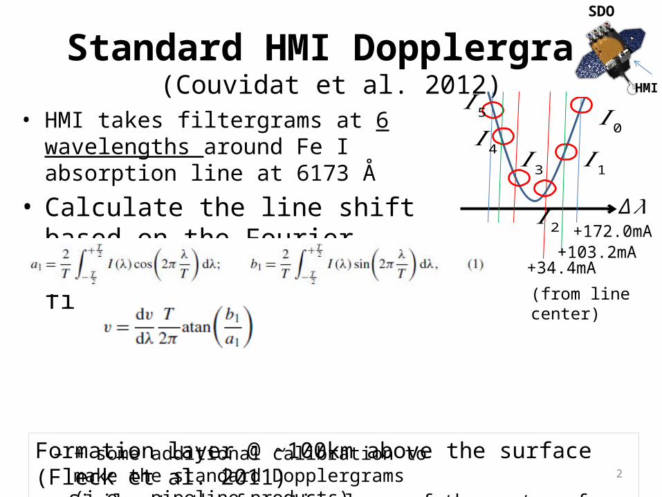
Standard HMI Dopplergram(Couvidat et al. 2012)

• HMI takes filtergrams at 6 wavelengths around Fe I absorption line at 6173 Å

• Calculate the line shift based on the Fourier coefficients of the 6 filtergrams

– + some additional calibration to make the standard Dopplergrams (i.e., pipeline products)

2

Δ 𝜆

Formation layer @ ~100km above the surface (Fleck et al. 2011)Similar to the formation layer of the center of gravity of the 6 filtergrams.

+172.0mA

HMI

SDO

𝐼 0𝐼 3 𝐼 1

𝐼 4

𝐼 5

𝐼 2

+34.4mA+103.2mA

(from line center)

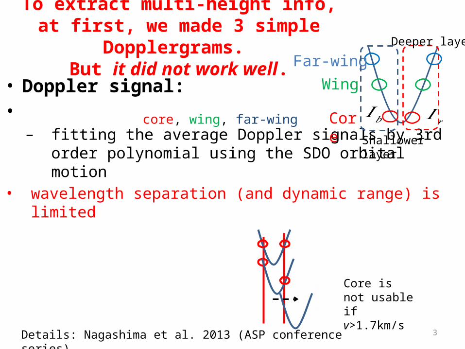
To extract multi-height info,at first, we made 3 simple Dopplergrams.

But it did not work well.• Doppler signal:• – fitting the average Doppler signals by 3rd order polynomial using

the SDO orbital motion • wavelength separation (and dynamic range) is limited

3

𝐼 𝑟𝐼𝑏Core

WingFar-wing

Deeper layer

Shallower layer

core, wing, far-wing

Details: Nagashima et al. 2013 (ASP conference series)

！Core is not usable if v>1.7km/s

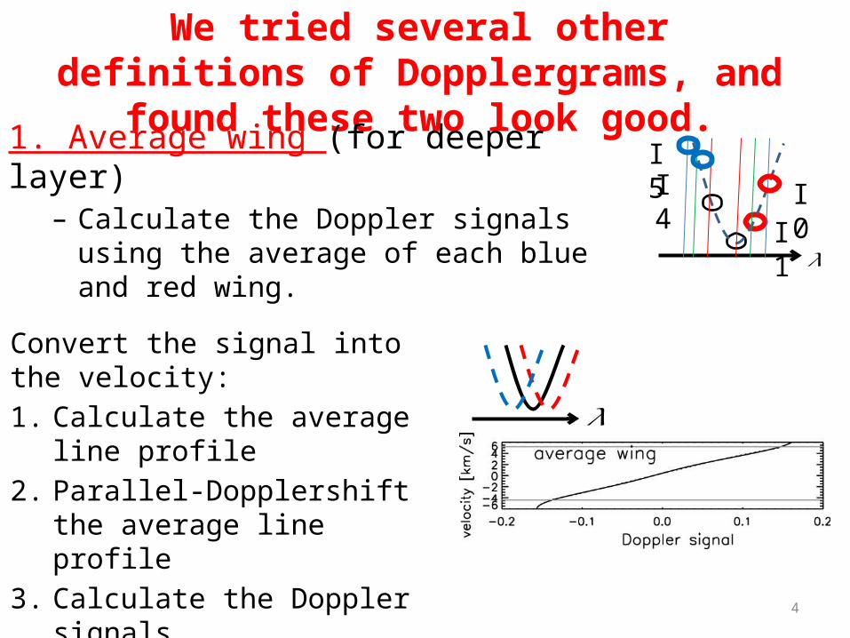
We tried several other definitions of Dopplergrams, and found these two look good.

1. Average wing (for deeper layer)– Calculate the Doppler signals using the

average of each blue and red wing.

4

𝜆

I5I0I4

I1

𝜆

Convert the signal into the velocity:1. Calculate the average line profile2. Parallel-Dopplershift the average

line profile3. Calculate the Doppler signals4. Fit to a polynomial function of the

signal

5

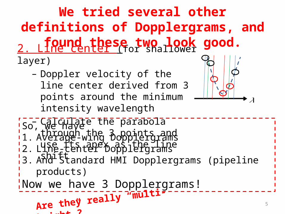
2. Line center (for shallower layer)– Doppler velocity of the line center

derived from 3 points around the minimum intensity wavelength

– Calculate the parabola through the 3 points and use its apex as the line shift

𝜆

So, we have 1. Average-wing Dopplergrams2. Line-center Dopplergrams3. And Standard HMI Dopplergrams (pipeline products)Now we have 3 Dopplergrams!

Are they really “multi-height”?

We tried several other definitions of Dopplergrams, and found these two look good.

Are they really “multi-height” Dopplergrams?　 (1) Estimate of the “formation height” using

simulation datasets (STAGGER/MURaM)

6

Are they really “multi-height” Dopplergrams?　 (1)Estimate of the “formation height” using simulation ⇒

datasets1. Use the realistic convection simulation

datasets: STAGGER (e.g., Stein 2012) and MURaM (Vögler et al. 2005)

2. Synthesize the Fe I 6173 absorption line profile using SPINOR code (Frutiger et al. 2000)

3. Synthesize the HMI filtergrams using the line profiles, HMI filter profiles, and HMI PSF

4. Calculate three Dopplergrams:Line center & Average wing & standard HMI

5. Calculate correlation coefficients between the synthetic Doppler velocities and the velocity in the simulation box 7

8

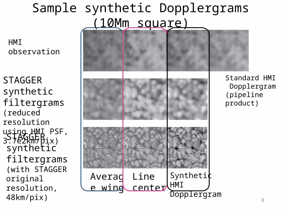
Sample synthetic Dopplergrams (10Mm square)

HMI observation

Average wing

Line center

Synthetic HMI Dopplergram

Standard HMI Dopplergram(pipeline product)

STAGGER synthetic filtergrams(reduced resolution using HMI PSF, 3.7e2km/pix)

STAGGER synthetic filtergrams (with STAGGER original resolution, 48km/pix)

Estimate of the “formation height” using simulation datasetsCorrelation coefficients between the synthetic Doppler velocities and

the velocity in the simulation box

9

Correlation coefficients

Peak heights：Line center 221km Standard HMI 195 kmAverage wing 170 km

Line center Standard HMI

Average wing

26km25km

10

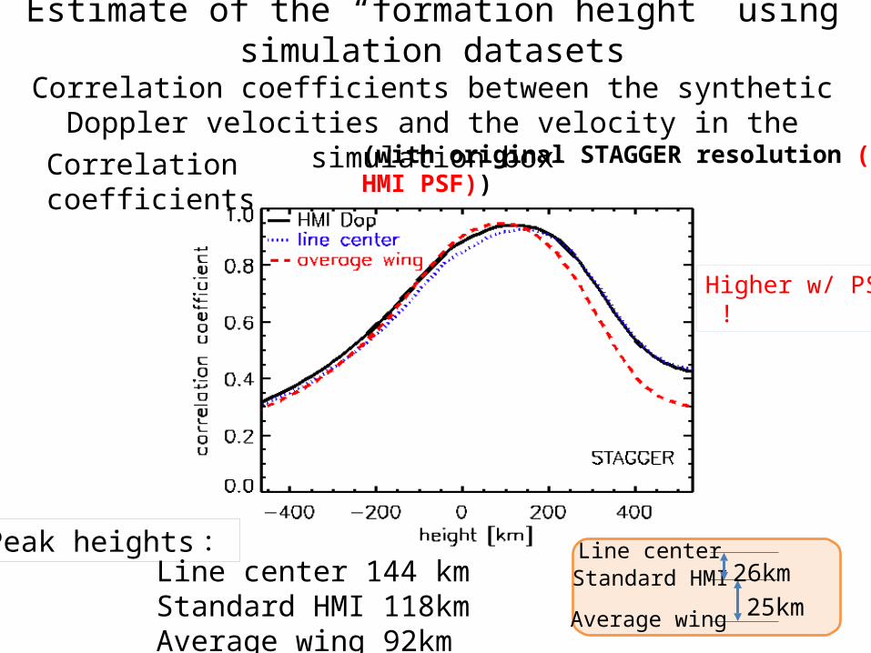
Higher w/ PSF !

(with original STAGGER resolution (no HMI PSF))

Estimate of the “formation height” using simulation datasetsCorrelation coefficients between the synthetic Doppler velocities and

the velocity in the simulation box

Correlation coefficients

Peak heights：Line center 144 km Standard HMI 118kmAverage wing 92km

Line center Standard HMI

Average wing

26km25km

11

17.6km/pix

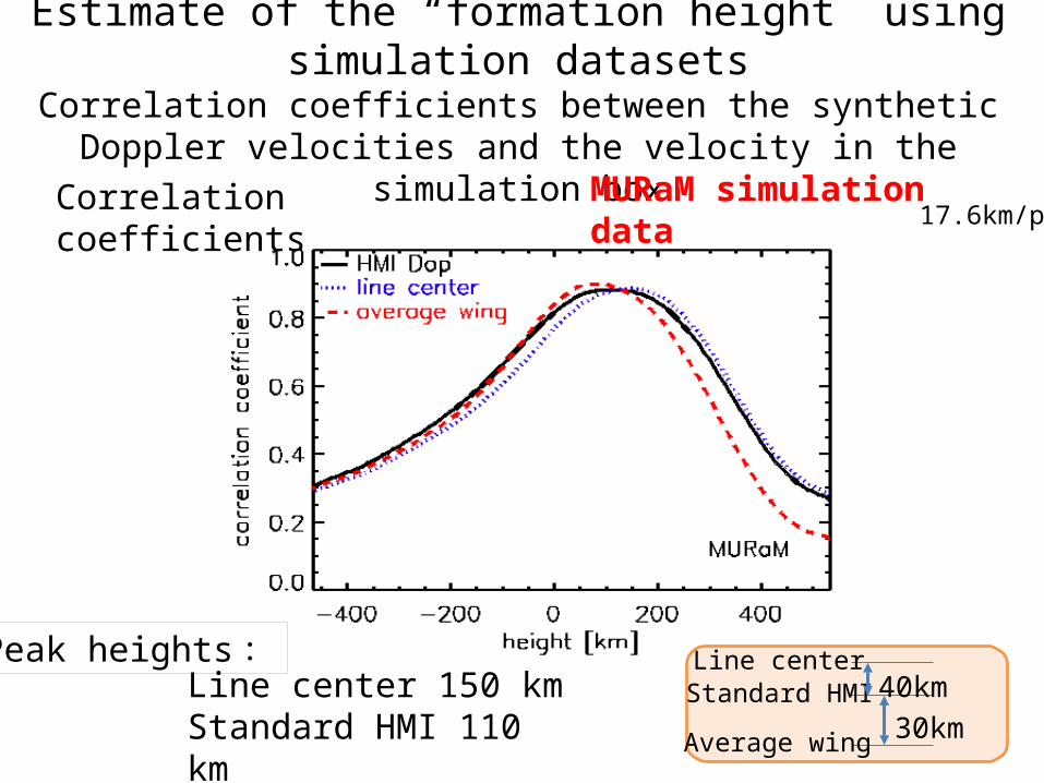
Estimate of the “formation height” using simulation datasetsCorrelation coefficients between the synthetic Doppler velocities and

the velocity in the simulation box

Correlation coefficients MURaM simulation data

Peak heights：Line center 150 km Standard HMI 110 kmAverage wing 80 km

Line center Standard HMI

Average wing

40km30km

The width of the correlation peak is so large.

12

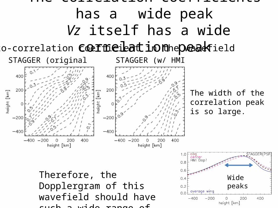
The correlation coefficients has a　 wide peak

Vz itself has a wide correlation peakSTAGGER (original resolution) STAGGER (w/ HMI PSF)

Wide peaksTherefore, the Dopplergram of this wavefield should have such a wide range of contribution heights.

Vz auto-correlation coefficient in the wavefield

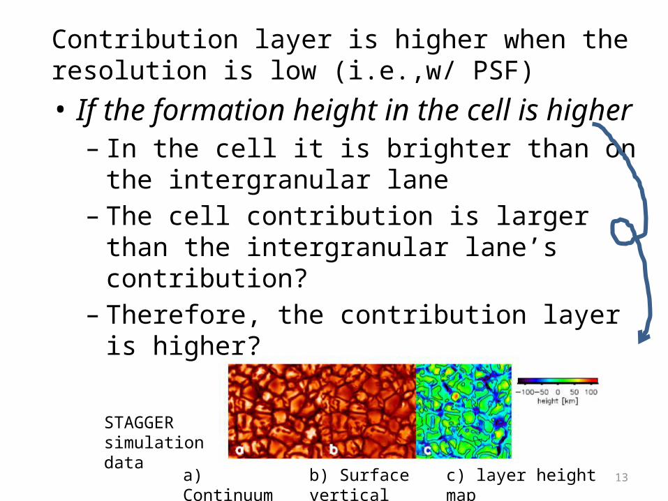
Contribution layer is higher when the resolution is low (i.e.,w/ PSF)• If the formation height in the cell is higher– In the cell it is brighter than on the intergranular

lane– The cell contribution is larger than the

intergranular lane’s contribution? – Therefore, the contribution layer is higher?

13a) Continuum intensity map

STAGGER simulation data

b) Surface vertical velocity map

c) layer height map

Are they really “multi-height” Dopplergrams?　 (2)

Phase difference measurements

14

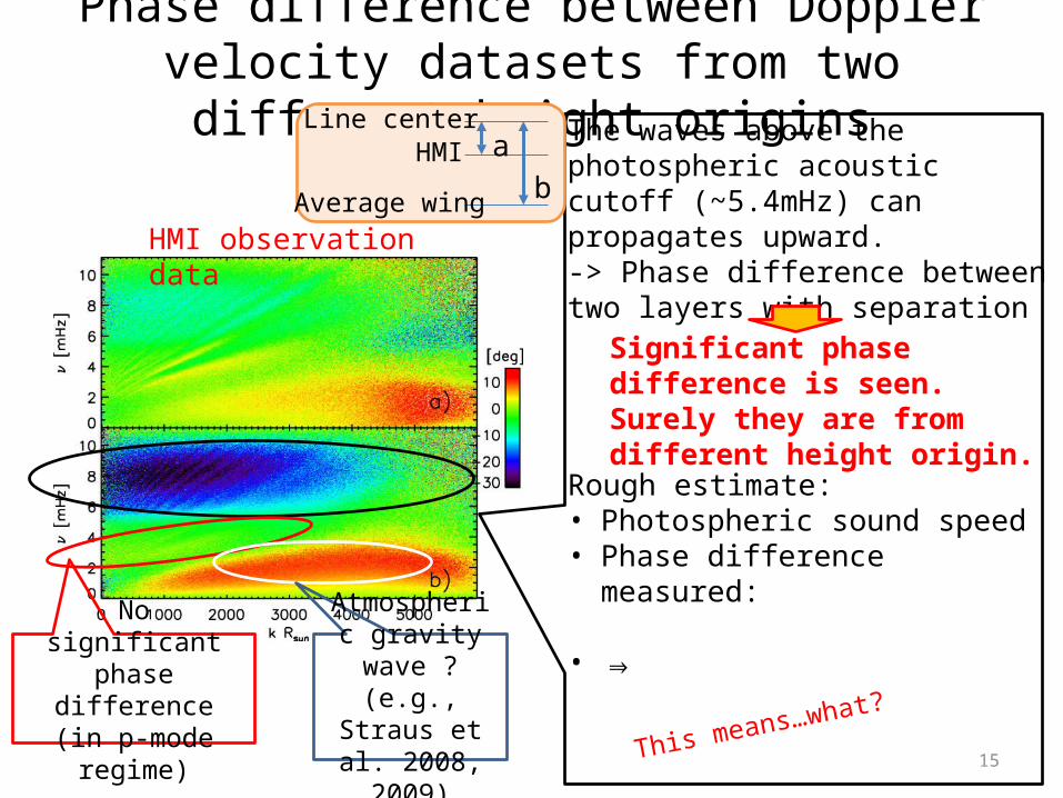
Phase difference between Doppler velocity datasets from two different height origins

15

The waves above the photospheric acoustic cutoff (~5.4mHz) can propagates upward.-> Phase difference between two layers with separation

Rough estimate:• Photospheric sound speed • Phase difference measured:

• ⇒　

No significant phase difference (in p-mode regime)

Atmospheric gravity wave ? (e.g., Straus et al. 2008, 2009)

Significant phase difference is seen.Surely they are from different height origin.

HMI observation data

Line center HMI

Average wing

ab

This means…what?

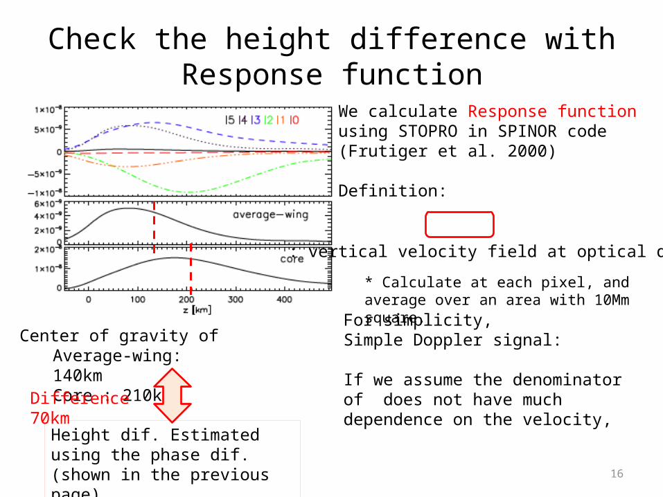
Check the height difference withResponse function

16

We calculate Response function using STOPRO in SPINOR code (Frutiger et al. 2000)

Definition:

: vertical velocity field at optical depth

For simplicity,Simple Doppler signal:

If we assume the denominator of does not have much dependence on the velocity,

Center of gravity of Average-wing: 140kmCore : 210km

Difference 70km

Height dif. Estimated using the phase dif. (shown in the previous page)

* Calculate at each pixel, and average over an area with 10Mm square.

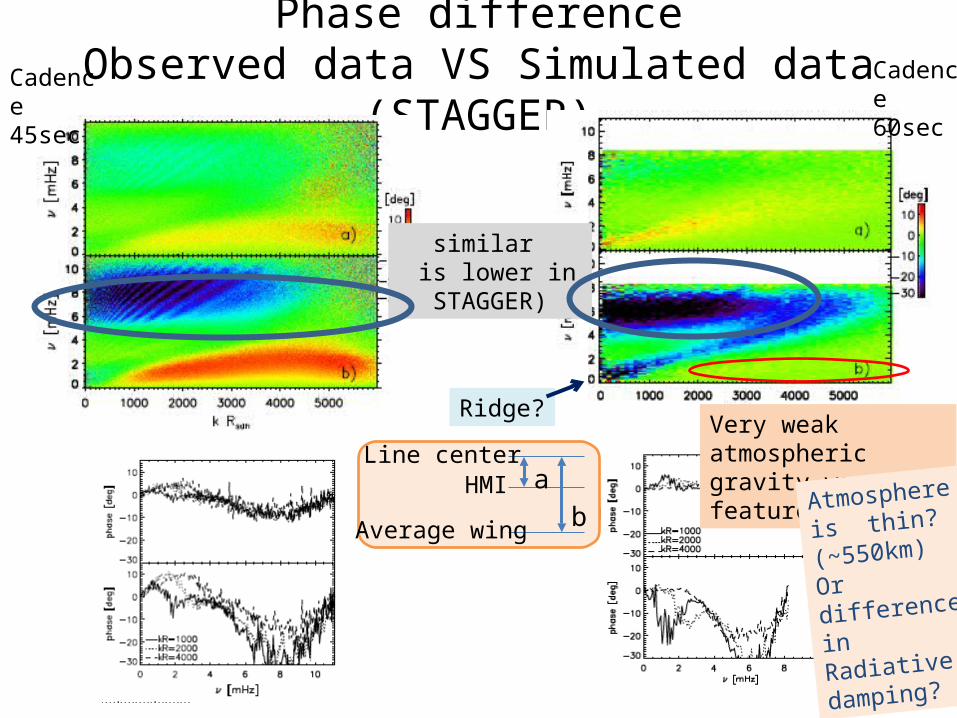
Phase differenceObserved data VS Simulated data (STAGGER)

17

Line center HMI

Average wing

ab

similar is lower in STAGGER)

Very weak atmospheric gravity wave feature

Ridge?

Cadence 60sec

Cadence 45sec

Atmosphere is

thin? (~550km)

Or difference in

Radiative

damping?

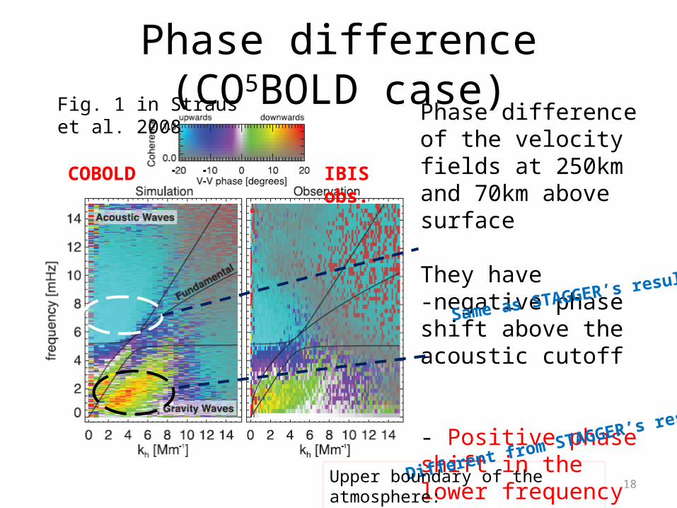
Phase difference (CO5BOLD case)Fig. 1 in Straus et al. 2008

18

IBIS obs. COBOLD

Phase difference of the velocity fields at 250km and 70km above surface

They have -negative phase shift above the acoustic cutoff

- Positive phase shift in the lower frequency ranges (atmospheric gravity waves)

Same as STAGGER’s results

Different from STAGGER’s results

Upper boundary of the atmosphere:STAGGER 550km, CO5BOLD 900km

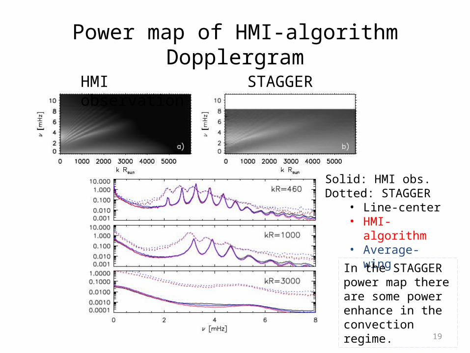
Power map of HMI-algorithm Dopplergram

19

HMI observation STAGGER

Solid: HMI obs.Dotted: STAGGER

• Line-center• HMI-algorithm• Average-wing

In the STAGGER power map there are some power enhance in the convection regime.

So… summary of the phase difference• P-mode regime: phase difference is small because they are

eigenmonds.

• : upward-propagating wave– phase difference found in observation data and STAGGER data have similar

trends.– in STAGGER atmosphere is lower than that of the Sun.

• Convective regime (lower frequency, larger wavenumber)– Observation: positive phase difference indicates the atmospheric gravity

waves– STAGGER : no such feature

• Atmospheric extent (about 550km) of STAGGER data might not be sufficient for the atmospheric gravity waves?

• Radiative damping of the short-wavelength waves in the STAGGER is stronger than the Sun?

• or…?20

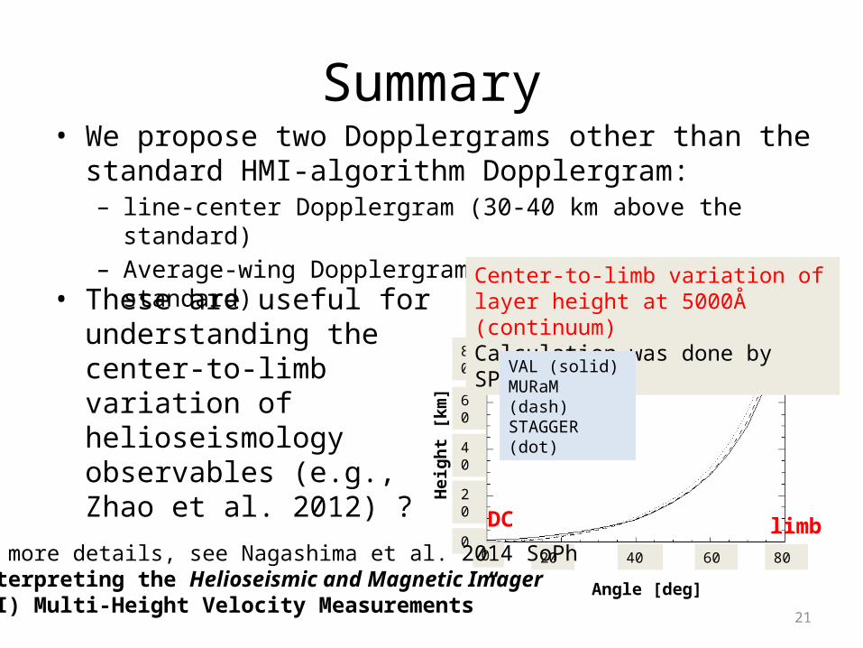
Summary• We propose two Dopplergrams other than the standard HMI-

algorithm Dopplergram:– line-center Dopplergram (30-40 km above the standard)– Average-wing Dopplergram (30-40 km below the standard)

0

20

40

60

80

20 40 60 80

Angle [deg]

0

Center-to-limb variation of layer height at 5000Å (continuum) Calculation was done by SPINOR code

VAL (solid)MURaM (dash)STAGGER (dot)

DC limb

• These are useful for understanding the center-to-limb variation of helioseismology observables (e.g., Zhao et al. 2012) ?

Hei

ght [

km]

21

For more details, see Nagashima et al. 2014 SoPh“Interpreting the Helioseismic and Magnetic Imager(HMI) Multi-Height Velocity Measurements”

22