script - W-GeoSoft · 5.3 Seismic receivers ... Seismic data processing. ... The aim of this lecture is to discuss the basic

Version (04.02.2005)

Reflexionsseismik 1 Seite 3

Version (04.02.2005)

Literature . . . . . . . . . . . . . . . . . . . . . . . . . . . . . . . . . . . . . . . . . . . . . . . . . . . . . . . . . . . . . . . . 5

1. Introduction . . . . . . . . . . . . . . . . . . . . . . . . . . . . . . . . . . . . . . . . . . . . . . . . . . . . . . . . . . . . 71.1 What is reflection seismics? . . . . . . . . . . . . . . . . . . . . . . . . . . . . . . . . . . . . . . . . . . . . . 71.2 Historical developments . . . . . . . . . . . . . . . . . . . . . . . . . . . . . . . . . . . . . . . . . . . . . . . . 81.3 Use of reflection seismics. . . . . . . . . . . . . . . . . . . . . . . . . . . . . . . . . . . . . . . . . . . . . . . . 9

2. Seismic waves. . . . . . . . . . . . . . . . . . . . . . . . . . . . . . . . . . . . . . . . . . . . . . . . . . . . . . . . . . . 102.1 Principles of wave propagation . . . . . . . . . . . . . . . . . . . . . . . . . . . . . . . . . . . . . . . . . . 112.2 Interface: reflection, refraction, conversion. . . . . . . . . . . . . . . . . . . . . . . . . . . . . . . . . 122.3 Reflection- and transmission coefficients . . . . . . . . . . . . . . . . . . . . . . . . . . . . . . . . . . 132.4 Geometry of wave propagation: rays . . . . . . . . . . . . . . . . . . . . . . . . . . . . . . . . . . . . . . 14

3. Seismic Velocities . . . . . . . . . . . . . . . . . . . . . . . . . . . . . . . . . . . . . . . . . . . . . . . . . . . . . . . 21

4. Amplitudes and Attenuation . . . . . . . . . . . . . . . . . . . . . . . . . . . . . . . . . . . . . . . . . . . . . . 25

5. Seismic data acquisition systems . . . . . . . . . . . . . . . . . . . . . . . . . . . . . . . . . . . . . . . . . . . 275.1 Introduction . . . . . . . . . . . . . . . . . . . . . . . . . . . . . . . . . . . . . . . . . . . . . . . . . . . . . . . . . 275.2 Seismic sources . . . . . . . . . . . . . . . . . . . . . . . . . . . . . . . . . . . . . . . . . . . . . . . . . . . . . . 275.3 Seismic receivers . . . . . . . . . . . . . . . . . . . . . . . . . . . . . . . . . . . . . . . . . . . . . . . . . . . . . 275.4 Registration unit . . . . . . . . . . . . . . . . . . . . . . . . . . . . . . . . . . . . . . . . . . . . . . . . . . . . . . 32

6. Acquisition setup . . . . . . . . . . . . . . . . . . . . . . . . . . . . . . . . . . . . . . . . . . . . . . . . . . . . . . . . 356.1 Single-channel measurements (Seismic profiling) . . . . . . . . . . . . . . . . . . . . . . . . . . . 356.2 Multi-channel measurements . . . . . . . . . . . . . . . . . . . . . . . . . . . . . . . . . . . . . . . . . . . . 356.3 CDP, CMP und Zero-Offset, Common offset . . . . . . . . . . . . . . . . . . . . . . . . . . . . . . . 36

7. Seismogram . . . . . . . . . . . . . . . . . . . . . . . . . . . . . . . . . . . . . . . . . . . . . . . . . . . . . . . . . . . . 387.1 The seismic trace . . . . . . . . . . . . . . . . . . . . . . . . . . . . . . . . . . . . . . . . . . . . . . . . . . . . . 387.2 Events in a seismic trace. . . . . . . . . . . . . . . . . . . . . . . . . . . . . . . . . . . . . . . . . . . . . . . . 407.3 Resolution . . . . . . . . . . . . . . . . . . . . . . . . . . . . . . . . . . . . . . . . . . . . . . . . . . . . . . . . . . 41

8. Basic scheme for processing of reflection data . . . . . . . . . . . . . . . . . . . . . . . . . . . . . . . . 438.1 Aim of data processing: . . . . . . . . . . . . . . . . . . . . . . . . . . . . . . . . . . . . . . . . . . . . . . . . 438.2 Basic framework fordata processing . . . . . . . . . . . . . . . . . . . . . . . . . . . . . . . . . . . . . . 43

9. Loading the data, Demultiplexing, Data-Format . . . . . . . . . . . . . . . . . . . . . . . . . . . . . 449.1 Principle of demultiplexing (Sorting of the data) . . . . . . . . . . . . . . . . . . . . . . . . . . . . 449.2 Dataformats . . . . . . . . . . . . . . . . . . . . . . . . . . . . . . . . . . . . . . . . . . . . . . . . . . . . . . . . . 44

10. Amplitude correction . . . . . . . . . . . . . . . . . . . . . . . . . . . . . . . . . . . . . . . . . . . . . . . . . . . 4610.1 Introduction . . . . . . . . . . . . . . . . . . . . . . . . . . . . . . . . . . . . . . . . . . . . . . . . . . . . . . . . 4610.2 Trace equalisation . . . . . . . . . . . . . . . . . . . . . . . . . . . . . . . . . . . . . . . . . . . . . . . . . . . 4610.3 Automatic Gain Control - AGC . . . . . . . . . . . . . . . . . . . . . . . . . . . . . . . . . . . . . . . . 4610.4 Spherical divergence correction . . . . . . . . . . . . . . . . . . . . . . . . . . . . . . . . . . . . . . . . 4710.5 Programmable gain curves (time and Distance-dependent) . . . . . . . . . . . . . . . . . . . 47

11. Filter (Frequencyfilter) . . . . . . . . . . . . . . . . . . . . . . . . . . . . . . . . . . . . . . . . . . . . . . . . . 4911.1 Fourier transformation . . . . . . . . . . . . . . . . . . . . . . . . . . . . . . . . . . . . . . . . . . . . . . . . 4911.2 Spectrumanalysis . . . . . . . . . . . . . . . . . . . . . . . . . . . . . . . . . . . . . . . . . . . . . . . . . . . . 4911.3 High cut, low cut, Band pass filter . . . . . . . . . . . . . . . . . . . . . . . . . . . . . . . . . . . . . . 50

12. Static corrections - Part 1 (Refraction) . . . . . . . . . . . . . . . . . . . . . . . . . . . . . . . . . . . . 5212.1 Introduction . . . . . . . . . . . . . . . . . . . . . . . . . . . . . . . . . . . . . . . . . . . . . . . . . . . . . . . . 5212.2 Methods for static correction . . . . . . . . . . . . . . . . . . . . . . . . . . . . . . . . . . . . . . . . . . . 53

Seite 4 Reflexionsseismik 1

Version (04.02.2005)

13. Deconvolution . . . . . . . . . . . . . . . . . . . . . . . . . . . . . . . . . . . . . . . . . . . . . . . . . . . . . . . . . 5413.1 Convolution . . . . . . . . . . . . . . . . . . . . . . . . . . . . . . . . . . . . . . . . . . . . . . . . . . . . . . . . 5413.2 Cross-correlation . . . . . . . . . . . . . . . . . . . . . . . . . . . . . . . . . . . . . . . . . . . . . . . . . . . . 5513.3 Deconvolution . . . . . . . . . . . . . . . . . . . . . . . . . . . . . . . . . . . . . . . . . . . . . . . . . . . . . . 56

14. Velocity analysis and NMO-Correction . . . . . . . . . . . . . . . . . . . . . . . . . . . . . . . . . . . . 5814.1 Normal-Moveout-Correction (NMO) . . . . . . . . . . . . . . . . . . . . . . . . . . . . . . . . . . . . 5814.2 Methods for velocity analysis . . . . . . . . . . . . . . . . . . . . . . . . . . . . . . . . . . . . . . . . . . 5914.3 Problem of stretching the data caused by NMO-correction . . . . . . . . . . . . . . . . . . . 6114.4 Factors influencing velocity estimates . . . . . . . . . . . . . . . . . . . . . . . . . . . . . . . . . . . . 62

15. Stacking . . . . . . . . . . . . . . . . . . . . . . . . . . . . . . . . . . . . . . . . . . . . . . . . . . . . . . . . . . . . . . 6315.1 Muting . . . . . . . . . . . . . . . . . . . . . . . . . . . . . . . . . . . . . . . . . . . . . . . . . . . . . . . . . . . . 6315.2 Methods of stacking . . . . . . . . . . . . . . . . . . . . . . . . . . . . . . . . . . . . . . . . . . . . . . . . . 63

16. Residual statics . . . . . . . . . . . . . . . . . . . . . . . . . . . . . . . . . . . . . . . . . . . . . . . . . . . . . . . . 6416.1 Principle of residual statics . . . . . . . . . . . . . . . . . . . . . . . . . . . . . . . . . . . . . . . . . . . . 64

17. Special Filters . . . . . . . . . . . . . . . . . . . . . . . . . . . . . . . . . . . . . . . . . . . . . . . . . . . . . . . . . 6517.1 Fk-Filter . . . . . . . . . . . . . . . . . . . . . . . . . . . . . . . . . . . . . . . . . . . . . . . . . . . . . . . . . . . 6517.2 τ-p-Filter . . . . . . . . . . . . . . . . . . . . . . . . . . . . . . . . . . . . . . . . . . . . . . . . . . . . . . . . . . 67

18. Migration . . . . . . . . . . . . . . . . . . . . . . . . . . . . . . . . . . . . . . . . . . . . . . . . . . . . . . . . . . . . . 6918.1 Geometrical distortion . . . . . . . . . . . . . . . . . . . . . . . . . . . . . . . . . . . . . . . . . . . . . . . . 7018.2 Methods for migration . . . . . . . . . . . . . . . . . . . . . . . . . . . . . . . . . . . . . . . . . . . . . . . . 7218.3 Special migration and extensions . . . . . . . . . . . . . . . . . . . . . . . . . . . . . . . . . . . . . . . 73

19. Postprocessing . . . . . . . . . . . . . . . . . . . . . . . . . . . . . . . . . . . . . . . . . . . . . . . . . . . . . . . . . 7619.1 Time-dependent Frequencyfilter . . . . . . . . . . . . . . . . . . . . . . . . . . . . . . . . . . . . . . . . 7619.2 Deconvolution . . . . . . . . . . . . . . . . . . . . . . . . . . . . . . . . . . . . . . . . . . . . . . . . . . . . . . 7619.3 Coherencyfilter . . . . . . . . . . . . . . . . . . . . . . . . . . . . . . . . . . . . . . . . . . . . . . . . . . . . . 7619.4 Amplitude correction . . . . . . . . . . . . . . . . . . . . . . . . . . . . . . . . . . . . . . . . . . . . . . . . . 7719.5 Archiving of Data . . . . . . . . . . . . . . . . . . . . . . . . . . . . . . . . . . . . . . . . . . . . . . . . . . . 77

20. Interpretation . . . . . . . . . . . . . . . . . . . . . . . . . . . . . . . . . . . . . . . . . . . . . . . . . . . . . . . . . 7920.1 Mapping of geological structures . . . . . . . . . . . . . . . . . . . . . . . . . . . . . . . . . . . . . . . 7920.2 Seismic sequence-analysis . . . . . . . . . . . . . . . . . . . . . . . . . . . . . . . . . . . . . . . . . . . . . 8020.3 Seismic facies analysis . . . . . . . . . . . . . . . . . . . . . . . . . . . . . . . . . . . . . . . . . . . . . . . 8120.4 Interpretation of 3D-data . . . . . . . . . . . . . . . . . . . . . . . . . . . . . . . . . . . . . . . . . . . . . . 8220.5 Other Aspects of interpretation . . . . . . . . . . . . . . . . . . . . . . . . . . . . . . . . . . . . . . . . . 82

21. Other related Methods . . . . . . . . . . . . . . . . . . . . . . . . . . . . . . . . . . . . . . . . . . . . . . . . . . 8321.1 VSP - vertical seismic profiling . . . . . . . . . . . . . . . . . . . . . . . . . . . . . . . . . . . . . . . . 8321.2 Cross-hole seismic . . . . . . . . . . . . . . . . . . . . . . . . . . . . . . . . . . . . . . . . . . . . . . . . . . . 8521.3 Sidescan sonar . . . . . . . . . . . . . . . . . . . . . . . . . . . . . . . . . . . . . . . . . . . . . . . . . . . . . . 8621.4 Georadar . . . . . . . . . . . . . . . . . . . . . . . . . . . . . . . . . . . . . . . . . . . . . . . . . . . . . . . . . . 8621.5 New developments . . . . . . . . . . . . . . . . . . . . . . . . . . . . . . . . . . . . . . . . . . . . . . . . . . . 86

22. Selection of used references (Figures etc.) . . . . . . . . . . . . . . . . . . . . . . . . . . . . . . . . . . 87

Reflection seismics 1 Page 5

Version (04.02.2005)

Literature

Seismics:Hatton, L., Worthington, M.H. and Makin, J. (1986). Seismic data processing - Theory and

practice. Blackwell Scientific publications, Oxford, UK, 177 pp.

Sheriff, E.G. and Geldart, L.P. (1995). Exploration Seismolgy, (2nd ed.). CambridgeUniversity Press, Cambridge, 592 pp.

Yilmaz, Ö. (1987). Seismic data processing. SEG Tulsa, OK, 826 pp.

Yilmaz, Ö. (2001). Seismic data Analysis: Processing, Inversion, and Interpretation ofSeismic data. SEG Tulsa, OK, 2027 pp.

Interpretation of seismic data:Emery, D. and Myers (eds.) (1996). Sequence Stratigraphy. Blackwell Science, Oxford, UK,

297 pp.

McQuilin, R. et al. (1986). An introduction to seismic interpretation. Graham and TrotmanLtd., London, UK.

Applied Geophysics in general (with one part about Seismics):Dobrin, M.B. and Savit, C.H. (1988). Introduction to geophysical prospecting (4.ed).

McGraw-Hill Book Comany, Ney York, 867 pp.

Kearey, P. and Brooks, M. (2002). An introduction to geophysical prospecting. BlackwellScientific Publications, Oxford, 262 pp.

Reynolds, J.M. (1998). An introduction to applied and environmental geophysics. JohnWiley and sons, Chichester, UK, 796 pp.

Telford, W.M., Geldart, L.P. and Sheriff, R.E (1990). Applied Geophysics (2. ed.).Cambridge University Press, Cambridge, 770 pp.


Version (04.02.2005)

1. Introduction

The aim of this lecture is to discuss the basic principles of Reflection Seismics and to explainthe basic fundamentals.

Knowledge of the lectures “Allgemeine Geophysik I und II” is indispensable. Knowledge of the lecture “Digitale Verarbeitung seismischer Signale” is an advantage.

The topic reflection seismics is that large that only for some parts an extensive mathematicaldiscussion is carried out. Therefore, this lecture only discuss qualitatively several topics whichare important for the reflection seismics. An extensive treatment of specific processingsteps andthe mathematical background will be treated by “Praktikum zur Datenverarbeitung in derReflexionsseismik”.

1.1 What is Reflection seismics?

In seismics, the geology is examined using seismic waves. The aim is to recognize geologicalstructures and, if possible, to determine the material properties of the subsurface.

t t t t t tQSource Receiver Raw data

seismic Sectiongeological subsoil

Page 8 Reflection seismic 1

Version (04.02.2005)

1.2 Historical Developments

Table 1: Historical development of reflection seismics(Sheriff and Geldart, 1995)

1914 Mintrop’s mechanical seismograph 1954 Continuous velocity logging 1917 Fessenden patent on seismic method 1955 Moveable magnetic heads 1921 Seismic reflection work by Geological

Engineering Co. 1956 Central data processing

1923 Refraction exploration by Seismos in Mexico and Texas

1961 Analog deconvolution and velocity filtering

1925 Fan-shooting method Electrical refraction seismograph Radio used for communications and/or time-break

1963 Digital data recording

1926 Reflection correlation method 1965 Air-gun seismic source 1927 First well velocity survey 1967 Depth controllers on marine streamer 1929 Reflection dip shooting 1968 Binary gain 1931 Reversed refraction profiling

Use of uphole phoneTruck-mounted drill

1969 Velocity analysis

1932 Automatic gain control Interchangeable filters

1971 Instaneous floating-point amplifier

1933 Use of multiple geophones per group 1972 Surface-consistent statics Bright spot as hydrocarbon indicator

1936 Rieber sonographfirst reproducible recording

1974 Digitization in the field

1939 Use of closed loops to check misties 1975 Seismic stratigraphy 1942 Record sections

Mixing 1976 Three-dimensional surveying

Image-ray migration (depth migration) 1944 Large-scale marine surveying

Use of large patterns 1984 Amplitude variation with offset

Determining porosity from amplitude DMO (dip-moveout) processing

1947 Marine shooting with Shoran 1985 Interpretation workstations 1950 Common-midpoint method 1986 Toiving multiple streamers 1951 Medium-range radio navigation 1988 S-wave exploration

Autopicking ot 3-D volumes 1952 Analog magnetic recording 1989 Dip and azimuth displays 1953 Vibroseis recording

Weight-dropping 1990 Acoustic positioning of streamers

GPS satellite positioning


Version (04.02.2005)

1.3 Use of Reflection seismicReflection seismic tools are used in many different ways. Depending on the aim and the usedifferent depth of penetration and resolution are obtained.Applications that do not belong to the area of the classical seismic (e.g. Georadar, echolot) usereflection seismic principles (traveltime curves, filters etc.).

Table 2: Application of reflection seismic tools

Aim Penetration Depth

Oil/gas Exploration of layers 100 m - 5 km

Engineering geo-physics

GroundwaterPolutionArchaeological investigation

10-500 m

Earth Crust seismic Composition of Earth/Geodynamic 1-60 km

Measurements in water

Echo sounder,high resolution Seismics

~ 0 m<100 m

Georadar GPR Shallow investigation of the Earth 0.5-10 m


Version (04.02.2005)

2. Seismic waves

The basic of Seismics are the elastic waves, which include both P- and S-wavesAcoustic waves include only P-waves (in water)

(1) Body waves:P-Waves (also Longitudinal- or compression waves)S-Waves (also Transversal- or Shearwaves)

(2) Surface waves exist on the interface between two different media:Rayleigh-Waves (Surface seismic wave propagated along a free surface of a semiinfinite medium)Love-Waves (Surface seismic channel wave SH wave

Propagation of different waves


Version (04.02.2005)

2.1 Principles of wave propagationThe propagation of seismic waves is described by the wave equation. This wave equation canbe derived from the relation between tension, elasticity, Hook’s law and Newtons law. In threedimension the derivation of this wave equation is quite complicated. This is why a simplifiedmedium is assumed which exist only of one dimension. Newtons (second) law (in onedimension) is given by

where P is the acoustic pressure and Uz is the displacement and ρ is the mass density. The well-known formula F=m*a can be recognised in this equation and describes that a force acting on acertain mass results in an acceleration of that mass.Hooke’s law is given by

where κ is the compressibility an relates the stress (force per unit area) and strain (change ofdimensions or shape). The bulk modulus k is the reciprocal of the compressibility and is givenby

Combining these two equations we obtain the Acoustic wave equation:

w(t) is the source signal and v is the wavespeed which is given by

We will not use these expressions for the wave equation, because for most topics treated in thislecture, it is sufficient to consider the wave equations in a geometrical way, as wavefronts or asrays. The wave equation is mainly used for modelling and inversion of seismic waves. It will beshown that the wave velocities depend on the compressibility and the density.

z∂∂ P ρ–

t2

2

∂

∂ Uz=

z∂∂ Uz κ– P=

k 1κ---=

z2

2

∂

∂ P 1v2-----

t2

2

∂

∂ P– w t( )δ z( )–=

v 1ρκ

----------- kρ---= =


Version (04.02.2005)

2.2 Interface: Reflection, Refraction, Conversion.

When a wave encounters an interface three phenomena can occur:

(1) Reflection(2) Refraction(3) Conversion

Reflection • Angle of incidence = angle of reflection (α1 = α2)

Refraction (change of direction of a seismic ray upon passing into a medium with a differentvelocity.)

• Critical angle: α2 = 90°, the refracted ray grazes the surface of contact between two media

Conversion • Change at the interface of p->s or s->p • As well as refraction as reflection is possible.

Law of SnelliusFor all events at an interface the ratio, is always the same.This ratio is also called the Raypath parameter p. The general Form of Snell’s law is given by:

Interface: α=Angle of P-Waves, β=Angle of S-Waves.

α1vp1,vs1

α1

β2

vp2,vs2

β1

α2

s

p

p

p

s

α1sinα2sin--------------

v1v2-----=

α1sin90°sin---------------- αsin 1

v1v2-----= =

αsinv-----------

α1sinvp1

--------------β1sin

vs1-------------

α2sinvp2

-------------- β2sinvs2

-------------- p const= = = = =


Version (04.02.2005)

2.3 Reflection- and transmission-coefficients

To derive the reflection and transmission coefficients for elastic waves, the boundary conditionsat the interface are needed. These reflections coefficients depend on• Difference in density • Difference in velocity• Angle of incident of the waveand are described by the Zoeppritz-Equations.

The Reflection- and Transmissioncoefficient give the ratio between the incident amplitude A0 ,and the reflected (AR) and transmitted (AT) amplitude, respectively. In the special case of aincident wave perpendicular at an interface for a P-wave, a simple expressions for the reflectionand transmission coefficient is obtained.

Reflectioncoefficient:

Transmissioncoefficient:

The Product is introduced as the acoustic Impedance.

Sometimes the coefficients which describe the Energy and not the amplitudes are introduced asReflection- und Transmissioncoefficients:

Reflection coefficient:

Transmission coefficient:

Obviously the total amount of energy is the same before and after the reflection and transmis-sion, so that :

In a general case these coefficients are depending on the angle of incidence. Moreover, alsoconversions between P- and S-waves occur at an interface. This results in complicated expres-sions which will not be discussed in this report.

RARA0-------

v2ρ2 v1ρ1–v2ρ2 v1ρ1+-----------------------------

Z2 Z1–Z2 Z1+------------------= = =

TATA0-------

2v1ρ1v2ρ2 v1ρ1+-----------------------------

2Z1Z2 Z1+------------------= = =

Z vρ=

ERZ2 Z1–( )2

Z2 Z1+( )2--------------------------=

ET4Z1Z2

Z2 Z1+( )2--------------------------=

ER ET+ 1=


Version (04.02.2005)

For the special case of v2/v1=2 and ρ2/ρ1=0.5, we have Z1=Z2. The P-wave reflection coeffi-cient is essentially zero for small angles of incidence. As the critical angle for P-waves isapproached, the transmitted P-wave energy falls rapidly to zero and no transmitted P-waveexists for larger incident angles.

2.4 Geometry of wave propagation: raysThe travel time can be derived by analysing the geometry of the rays that travel from source toreceiver (when the velocity and depth are known).

=> geometrical Seismic

Angle-dependent reflection- and transmission-coefficients for P- and S-waves


Version (04.02.2005)

Traveltime curveThe traveltime of the different rays are plotted in an x-t diagram, a Traveltime plot. The picturebelow shows such a traveltime plot.

The important rays in the travel time diagram are:• Direct wave• Reflected wave• Refracted wave

The separate elements will be discussed in the following paragraphs:

Direct waveThe direct wave travels only in the upper layer, directly from the source to the receiver. Whenthe upper layer has a homogeneous velocity distribution than we can assume that the wavetravels parallel to the interface. In the traveltime diagram the direct wave shows a slope of 1/v.

Reflected wave in the horizontal two-layer caseIn Reflection seismic this signal is investigated and used. Therefore, we discuss this wave inmore detail.

Picture of a typical travel time diagram for a two-layer case. t0 = t0-time of the Reflection; ti=Intercept-time of the Refraction; xcrit =critical distance;

xcross=”cross-over”-distance.

t0ti


Version (04.02.2005)

The simplest case is the horizontal two-layer configuration.

Using pythagoras we have:

which gives:

The traveltime of a reflected wave goes for large x asymptotically towards the traveltime of thedirect wave (t=x/v). Rewriting last equations renders:

This is the expression for a hyperbola.

The crossing with the time-Axis (x=0) is the timezero, t0:

Schematic overview to calculate the traveltime expressions for a reflection.

v

x/2 x/2A

C

B

αα

hs

o x

s

s2 h2 x2---⎝ ⎠

⎛ ⎞ 2+=

t2 4s2

v2-------- 4h2 x2+

v2---------------------= =

v2t2

4h2--------- x2

4h2--------– 1=

t0

t02v2 4h2 t x 0=( ) t0

2hv------= =⇒=


Version (04.02.2005)

With the t0-time the expression for the traveltime can be written as:

Moveout

Rewriting the former equation, and using a binomial expansion of the square root

.

we obtain an approximate expression for the moveout in time between two different positionsx1 and x2.

Normal MoveoutThe difference between the traveltime t for a specific receiver at a specific distance x and areceiver at zero-offset x0=0 is given by the normal moveout which is defined as:

This formula will later be used in the processing of seismic data.

t2 x2

v2----- t02+=

t2 t02 1 x2

t02v

2------------+⎝ ⎠⎜ ⎟⎛ ⎞

=

t t0 1 x2

t02v

2------------+⎝ ⎠⎜ ⎟⎛ ⎞

=

t t0 1 x2

2t02v

2---------------+⎝ ⎠⎜ ⎟⎛ ⎞

≈ t0x2

2t0v2-------------+=

t2 t1–x2

2 x12–

2t0v2---------------------=

∆T tx= t0x2

2v2t0

-------------≈–


Version (04.02.2005)

Reflections - horizontal layered mediumWhen more than two layers are present the rays of the reflections are more complex due to therefraction that occurs at each interface. With the help of Snell’s law an approximate estimate ofthe rays can be obtained iteratively..

It is possible to replace the expressions with the expressions for the one layer case when for thelayers above the actual reflection point an average velocity is assumed.A possible average velocity is given by.

where zi is the thickness of the ith layer, τi is the interval travel time through the ith layer and viis the velocity of the ith layer.For small offsets the travel-time curve is still essentially hyperbolic so that using the hyperbolicexpression an average velocity can be obtained for the layers above the actual reflection point.Therefore, a better approximation is obtained when instead of the arithmetic average, the arith-metic average is taken of the square of the velocities(“rms: root-mean-square”).

The so-called RMS-velocity is used for all velocity analysis of reflection data, because it isrelatively easy to obtain it from a seismogram.

The velocity that is used to remove the effect of normal moveout is called stacking velocity(This NMO-correction will be discussed later in more detail). Correcting for the moveout usingthe stacking velocity and stacking the traces results in the maximum amplitude of the reflectionevent. As mentioned before, the travel-time curve for reflected rays in a multi-layered groundis not a hyperbola. However, if the maximum offset is small compared with reflector depth, thestacking velocity closely approximates the root-mean-square velocity.

Three horizontal layers as example for a layered horizontal medium. The solid line representsthe real travelpath, where the dashed line represents the travel path of one layer with equaltravel time.

v1

v2

v3

vaverage

viτi

i 1=

n

∑

τi

i 1=

n

∑

------------------=

vrms2

vi2τi

i 1=

n

∑

τi

i 1=

n

∑

---------------------=


Version (04.02.2005)

To calculate the interval-velocities from the RMS-velocities, the Formula of Dix is used:

vi is the intervalvelocity of the nth layer. tn is the measured traveltime to the nth layer. When(travel time for zero offset) we assume that the travel path to the individual reflections

are equal. This is in general not correct. Dix’ Formula can then result in wrong vi - values.

Reflection from a dipping reflectorThe reflectors in reality are often not horizontal but dipping.

With the help of the cosinus rule an expression for the traveltimes can be derived as follows:

The derivation of the next formulas for the dipping reflector follows analogue the case of thehorizontal layer, with the exception that the expressions include a term with the angle Θ. Weobtain a hyperbolic expression:

Where the symmetry axis does not lie on the t-axis, but is now the line .

Ray path and traveltime diagram for a dipping Reflektor.

vivrmsn

2 tn vrmsn 1–

2 tn 1––tn tn 1––--------------------------------------------------

12---

=

tn t0n≠

x 90 + Θ

Θ

h

h

∆Tdip

x-x

v2t2 x2 4h2 4hx 90 Θ+( )cos⋅–+=v2t2 x2 4h2 4hx Θsin⋅+ +=

v2t2

2h Θcos( )2--------------------------- x 2h Θsin+( )2

2h Θcos( )2-----------------------------------– 1=

x 2– h Θsin=

v2t2 2h Θcos( )2 x 2h Θsin+( )2+=

t2 2h( )2

v2------------- 1 x 2h Θsin+( )2

4h2-----------------------------------+=


Version (04.02.2005)

(Where cosΘ is assumed to be 1 for small angles). After expansion as a binomial expression we obtain:

where t0 is given by

The traveltime from two locations x und -x, that both have the same distance from the shotposition is not equal anymore caused by the dipping reflector. The traveltime differencebetween both points is called the “dip-moveout”.

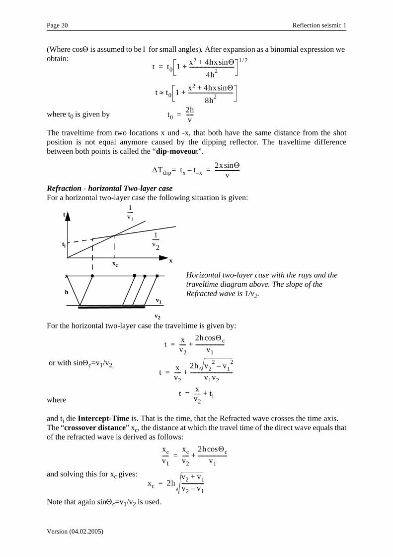
Refraction - horizontal Two-layer caseFor a horizontal two-layer case the following situation is given:

For the horizontal two-layer case the traveltime is given by:

or with sinΘc=v1/v2,

where

and ti die Intercept-Time is. That is the time, that the Refracted wave crosses the time axis. The “crossover distance” xc, the distance at which the travel time of the direct wave equals thatof the refracted wave is derived as follows:

and solving this for xc gives:

Note that again sinΘc=v1/v2 is used.

t t0 1 x2 4hx Θsin+4h2----------------------------------+

1 2/=

t t0 1 x2 4hx Θsin+8h2----------------------------------+≈

t02hv------=

∆Tdip tx t x––= 2x Θsinv-------------------=

v1

x

v2

ti

h

xcx

t

1v2------

Horizontal two-layer case with the rays and the traveltime diagram above. The slope of the Refracted wave is 1/v2.

1v1-----

t xv2-----

2h Θccosv1

----------------------+=

t xv2-----

2h v22 v1

2–v1v2

--------------------------------+=

t xv2----- ti+=

xcv1-----

xcv2-----

2h Θccosv1

----------------------+=

xc 2hv2 v1+v2 v1–-----------------=


Version (15.02.2005)

3. Seismic Velocities

The velocities is the most important parameter in reflection seismics. Information about thevelocities is important for:

• Change of traveltime with depth• Check of the seismic data with a model• Correct for the geometry (Migration)• Classification and filtering of signal and noise• Geological and lithological Interpretation

The seismic velocity depends on the elastic parameters as follows:

with k= Bulk modulusµ = Shear modulus

From these equations we observe that:• vp is always larger than vs• In Liquids, µ = 0 => no shear waves can propagate.

Poisson-RatioThe Poisson-Ratio σ is the ratio of transverse strain to longitudinal strain and is defined as:

and has values between 0 < σ < 0.5 (0.5 is valid for fluids).

Seismic velocities and the factors influencing it.In Reality the factors k, µ and ρ depend in a complex way on different factors:

• Lithology (Matrix und Struktur)• Depth• Interstitial fluids• Pressure• Porosity• Degree of compaction• Cementation• etc.

Most of these factors influencing the factors k, µ and ρ are empirically determined.

vp

k 4µ3------+

ρ----------------=

vsµρ---=

σ 3k 2µ–2 3k µ+( )------------------------=


Version (15.02.2005)

Sum

mar

y of

effe

cts o

f diff

eren

t roc

k pr

oper

ties o

n P-

and

S-w

ave

velo

citie

s and

thei

r ra

tios.(

Sher

riff

and

Gel

dart

199

5).


Version (15.02.2005)

Examples for typical velocities

(Kearey and Brooks, 1991)

material vp (km s-1)

Unconsolidated MaterialSand (dry) 0.2 - 1.0Sand (water saturated) 1.5 - 2.0Clay 1.0 - 2.5Glacial till (water saturated) 1.5 - 2.5Permafrost 3.5 - 4.0

Sedimentary rocksSandstone 2.0 - 6.0

Tertiary sandstone 2.0 - 2.5Pennant sadstone (Carboiferous) 4.0 - 4.5Cambrian quartzite 5.5 - 6.0

Limestones 2.0 - 6.0Cretaceous chalk 2.0 - 2.5Jurassic oolites and bioclastic limstones 3.0 - 4.0Carbiniferous limestone 5.0 - 5.5Dolomites 2.5-6.5

Salt 4.5 - 5.0Anhydrite 4.5 - 6.5Gypsum 2.0 - 3.5

Igneous / Metamorphic rocksGranite 5.5 - 6.0Gabbro 6.5 - 7.0Ultramfic rocks 7.5 - 8.5Serpentinite 5.5 - 6,5

Pore fluidsAir 0.3Water 1.4 - 1.5Ice 3.4Petroleum 1.3 - 1.4

Other materialsSteel 6.1Iron 5.8Aluminium 6.6Concrete 3.6


Version (15.02.2005)

AnisotropySeismic velocities in a solid can depend on the direction in which they travel within the solid.(for example Granite). This is the case when the matrix in the solid is direction dependentcaused by for example gravitational forces .

Direct measurements of the seismic velocity

Velocities can be determined when measuring the time, that a seismic wave needs to travel acertain distance. Direct measurements are carried out in a laboratory in a small probe or in situin a borehole

Problem: Many times higher frequencies are used to determine the seismic velocities. It is important thatthe velocity is frequency dependent, especially in a heterogeneous solid.

Anisotropy: A seismic wave travels faster in that direction where the matrix is more dense.


Version (15.02.2005)

4. Amplitudes and Attenuation

The amplitudes of a seismic signal are influenced by several factors:

• Divergence• Absorption• Scattering of Energie at an interface

(Reflection, Refraction, Conversion)• Interference with other waves(e.g. multiple Reflections)• Spreading of Energie • Influence of measurement system

Spherical divergence (geometrical spreading)

When a seismic wave propagates, the energy is spread alongthe surface of the wavefront. For cylindrical and sphericalwaves the surface increases with increasing radius. That iswhy the energy decreases. The Energy of the different wavesare proportional to:

• plane Wave: konstant• cylindrical Wave: ~ 1/r• spherical Wave: ~ 1/r2

The energy of the body (spherical) and interface (cylindrical)waves are proportional to (1/r2) and (1/r), respectively. The amplitude of the body and interfacewaves are proportional to (1/r) and (1/or), respectively (energy is proportional to (amplitude)2).

Phenomena causing the degradation of a seismic wave (Reynolds, 1998).

r1

r2


Version (15.02.2005)

Absorption

When elastic waves travel through the subsurface, a part of their energy is dissipated in heat.The decrease of amplitude due to absorption appears to be exponential with distance for elasticwaves in rock which can be written as:

A and A0 are the amplitudes at two locations with a distance x and α is the absorptioncoeffi-cient.

Quality factor QThe absorption is often described by the Quality factor Q (Q-Factor) that is given by:

The absorption coefficient α can be considered as a first approximation proportional to thefrequency. We can write:

This is only valid for Q >> 1 (where v = Velocity and f = Frequency).

A A0e αx–=

Q 2π∆E( ) E⁄

-------------------- 2πFraction of Energie, lost per Cycle-------------------------------------------------------------------------------------= =

1Q----

αvπf------- αλ

π-------= =


Version (15.02.2005)

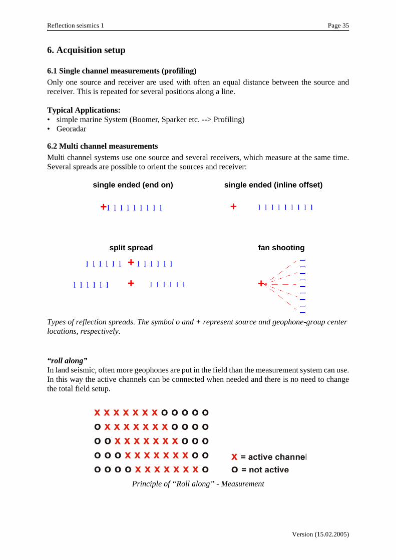
6. Acquisition setup

6.1 Single channel measurements (profiling)Only one source and receiver are used with often an equal distance between the source andreceiver. This is repeated for several positions along a line.

Typical Applications:• simple marine System (Boomer, Sparker etc. --> Profiling)• Georadar

6.2 Multi channel measurementsMulti channel systems use one source and several receivers, which measure at the same time.Several spreads are possible to orient the sources and receiver:

“roll along”In land seismic, often more geophones are put in the field than the measurement system can use.In this way the active channels can be connected when needed and there is no need to changethe total field setup.

Principle of “Roll along” - Measurement

Types of reflection spreads. The symbol o and + represent source and geophone-group center locations, respectively.

+l l l l l l l l l

single ended (end on)

split spread fan shooting

single ended (inline offset)

+ l l l l l l l l l

+l l l l l l l l l l l l

+l l l l l l l l l l l l +l

ll

ll

ll

ll


Version (15.02.2005)

6.3 CDP, CMP and Zero-Offset, Common offsetThere are different possibilities to sort the data:

• Common shot - all traces, that belong to the same shot • Common midpoint (CMP) - all traces with the same midpoint• Common receiver - all traces, recorded with the same geophone• Common offset - all traces with the same offset between shot and geophone

Common mid point - CMP

For a horizontal layerered earth the reflectionpoint lies between source and receiver (midpoint) Using more shots with different positions of the source and receivers several combinations ofsource and receivers exists which have the same midpoint. When a horizontal layering is presentthe reflection then also come from an equal point in the subsurface (Common depth point-CDP). For an inclined layer the point of reflection for traces with the same midpoint are notequal anymore. The nomenclature CDP is not valid anymore. However several processingprograms still use the word CDP in stead of CMP.

Zero offsetZero offset data is characterised when the source and receiver are present on the same location.There is no moveout. For a normal measurement this is seldom the case. When the traces arecorrected for the moveout and are stacked then a zero offset trace is obtained.

Difference between CMP und CDP: For a horizontal Reflector all traces that have the same midpoint, have also the same reflectionpoint in the subsurface. Is the layer inclined than the traces have a different reflectionpoint.


Version (15.02.2005)

Common offsetAll traces with equal offset between source and receiver. This configuration is often used forseveral Single channel systems. Also Georadar measurements are often carried out with a fixedoffset between source and receiver.

FoldThe fold indicates the number of traces per CDP. This is often the number of traces in a CMP.The theoretical formula for the fold is given by:

The number of traces which are measured at a certain geophone position is called “surface fold”

Crooked line method

Sometimes access and/or structural complications make it impossible to locate lines in desiredlocations. The field recording may be done in the same way as CMP surveying, except that theline is allowed to bend. Usually, a best-fit straight line is drawn through the midpoint plot,rectangular bins are constructed and those traces whose midpoints fall within a bin are stackedtogether. The bins are often perpendicular tot the final line, but sometimes bins are oriented inthe strike direction. Because the actual midpoint locations are distributed over an area, theycontain information about dip perpendicular to the line and in effect produce a series of cross-spreads, from which the true dip can be resolved. Lines are sometimes run crooked intentionallyto give cross-dip information.

3D-SeismicThe sources and receivers do not lie on a line, but in both horizontal directions sources andreceiver are placed. In this way not only for different offsets, but also information from differentdirections (azimuths) is obtained. Here also bins are defined and all traces of the specific CMPare gathered after processing in that bin.

Fold Numberof Geophones Distance between Geophones⋅2 Distance between shots⋅

--------------------------------------------------------------------------------------------------------------------------------------=


Version (15.02.2005)

7. Seismogram

7.1. The seismic TraceIn Seismic reflection surveys we measure the ground motion over a short interval of timefollowing the triggering of a nearby seismic source. The graphical plot of the output of a singledetector is called a Seismogram or seismic trace;

The properties of the geological subsoil (density and seismic velocity) determine the acousticimpedance of a layer. From these impedances the reflectivity function of an interface can bederived (see Chapter. 2). This function is convolved with the signal of the seismic wave. Theresult is a seismic trace, on which also noise is add.

Remark: note that the wave travels half of the time downwards and the other half upwards. Thismust be taken into account when the source signal is convolved with the reflectivity function.(The principle of convolution is discussed more thoroughly when the data processing isdiscussed).

WaveformThe most important waveforms in seismic are shown in the figure below and are the• Minimum-Phase wavelet• zero phase wavelet

From a geological subsoil to a seismic trace.


Version (15.02.2005)

RepresentationThe traveltime is in general shown with increasing time along the vertical increasingdownwards (larger traveltime corresponds to a larger depth).There are several ways to represent seismic traces. The sort of representation depend on theprocessing used, but also on the number of traces.

“Wiggle”For the simplest representation the amplitude is depicted as a curve (Wiggle). “Variable area+wiggle”When there are more traces then the result is disordered. The right half of the trace is drawnblack. Standard (set by SEG) is: the positive half of the wave on the right site is colored black.

The most important waveforms in seismics: (a) Minimum-Wavelet and (b) Zero-Phase Wavelet. Both waveforms are shown with normal and reverse polarity.

Different representations of a seismic trace.


Version (15.02.2005)

This is in seismics the most used representation.“Variable area”When a lot of traces are depicted close to each other, then most of the time only the positive halfof the traces is plotted. (e.g. for smaller version of seismic sections.). To suppress noise oneoften plot only a part of the half of the waves(Variable Amplitude).“Variable density”For the interpretation the amplitudes are often plotted in different grayscales or colours(“variable density”). This is standard for Georadar or seismic Interpretation. In this way thedifferences in amplitudes are more clear.

7.2 Events in a seismic traceThe important elements are• Reflections• Refractions• Interface waves• Multiples• NoiseReflections, Refractions and interface waves are already discussed in Chapter 2.

Multiples

1) long-path multiples (occur when exceptionally large reflectioncoefficients are present):-> Ghost reflections, where rays from a buried explosion on land (or an airgun in water) arereflected back from the ground surface (or sea surface) to produce a reflection event, known asa ghost reflection, that arrives a short time after the primary. -> Water layer reverberations, where rays from a marine source are repeatedly reflected at thesea bed and sea surface2) Short-part multiples (“peg-leg multiple”):Involve only a short additional path length to arrive so soon after the primary event that theyextend the overall length of the pulse. (Multiples between two interfaces of a layer)

Example for the travelpaths of multiple reflections.


Version (15.02.2005)

NoiseThe S/N ratio “Signal-to-noise ratio” gives the ratio between the amplitude of a signal (e.g.Reflections) to background noise(“random noise”) or noise sources (“coherent noise”).

One aim of the dataprocessing is to increase the S/N ratio.

7.3. Resolution

Vertical resolution

Vertical resolution means: How thick must a layer be, to discern the top and bottom of thespecific layer. Theoretically, a layer can be distinguished when it has a thickness of 1/4wavelength (Rayleigh-Kriterium).

The wavelength is determined by the ratio of the velocity and the frequency of the seismic wave:λ = v / f.

Lateral ResolutionThe lateral resolution depends on the distance between the source and receiver at the surfaceand the depth of the layer. Energy that is returned to a detector within half a wavelength of theinitial reflected arrival interferes constructively to build up the reflected signal, and the part ofthe interface from which this energy is returned is known as the first Fresnel zone, or, simply,Fresnel zone.The width of the Fresnel zone represents an absolute limit on the horizontal resolution of areflection survey since reflections separated by a distance smaller than this cannot be individ-ually distinguished. The width w of the Fresnel zone is related to the dominant wavelength λ ofthe source and the reflector depth z by

Comparison between the wavelength of a 30-Hz Signal, Big Ben and a Log of a drilling.


Version (15.02.2005)

for z>> λ.

Principle of the Fresnel-Zone

w 2zλ=


Version (15.02.2005)

11. Filter (Frequency filter)

Frequency filter are the most important filters in digital signal processing. The energy of reflec-tions are most of the time present in a certain frequency range. Specific noise sources andbackground noise are commonly present in a different frequency range and a separation of noiseand reflection information is possible.

11.1 Fourier transformationThe basis of a digital frequency filter is the Fourier transformation. The principle of Fouriersays that each signal can be described by a sum of Sinus- and Cosinus functions.The Fourier transformation transforms a time queue from time domain (amplitude as functionof time) to the frequency domain ( amplitude as function of frequency).

Fourier transformation: (from time to frequency)

Inverse Fourier transformation: (from frequency to time)

The Function in Frequency domain G(f) represents the amplitude and the phasedifference of aSinus or Cosinus function with the frequency f. We distinguish the Amplitude spectrum A(f)and the Phasespectrum φ(f):

Because in frequency domain the data consists of an amplitude and phase (or real and imagi-nairy part), often the amplitude spectrum of the energy, the “Powerspectrum” is shown. TheFourier transformation is numerically evaluated very efficiently by the FFT - the Fast FourierTransform.

11.2 SpectrumanalysisIn seismics, we often know only roughly the interesting frequency range and the frequencyrange of any noise sources. To know what frequency range is interesting for further processing,the data must be tested with different filters and a comparison of these results indicate the inter-esting frequency range.

G f( ) g t( )e i2πft– td∞–

∞

∫=

g t( ) G f( )ei2πft fd∞–

∞

∫=

Phase-Spectrum

Amplitude-Spectrum

g(t) G(f) = A(f) e iφ(f)

A(f)

φ(f)


Version (15.02.2005)

-.

11.3 High cut, Low cut, Band pass and Notch filterThere are different type of filters:• high cut, low pass• low cut, high pass• Bandpass • Notch filterMost filters are applied in the frequency domain. For example, using the Low pass filter, theamplitude of all frequencies above a certain frequency are put to zero. Similar filtering isapplied for the High pass and Band pass filters

Notch-FilterA notch-filter is used to suppress one specific frequency, for example 50-Hz-Noise due toelectrical powerlines.

Examples of different signals and their Fourier transformation.


Version (15.02.2005)

RingingIdeal filters have very steep edges, which is in the ideal case discontinuous.The result of such discontinuities is ringing (also known as Gibbs’ phenomena) as can be seenin the figure below. In figure (a), the frequency domain result is present with a discontinuity atfc. This discontinuity results in an oscillatory behaviour in the time domain as can be seen infigure (b). When a taper is used to make the transition more smooth at fc(c), the oscillarorybehaviour is less pronounced:

In practise, it is not possible to design a frequency filter which is discontinuous at the edges.To define this tapering a slope is given as function of the frequency as follows:• Two Frequencies in between the taper is present (Begin and End of the tapering)• The slope of the taper is given as function of the Frequency in dB

Examples of different type of filters.

Principle of ringing which occurs in time domain when sharp boundaries are present in the frequency domain.

Low pass High pass

Bandpass Notchfilter

100%

0%

100%

0%


Version (15.02.2005)

Time-dependent Frequency filterTo take into account the larger decrease in amplitude for the higher frequencies for increasingtravel time, a time-dependent frequency filter can be used. One defines different frequencyfilters for different timewindows.

12. Static Correction - Part 1 (Refraction)

12.1 IntroductionReflections in different traces are not always lying on a hyperbole for a horizontal reflector, butsometimes they have a certain displacement due to different lengths of the raypaths.

Causes for the static displacements in the data:• Topography, i.e. Source and receiver are present at different vertical positions.• Different depths of the boreholes in which the explosives were fired• Weathered layer with a relative slow velocity.

Effect of topography on measured data. The reflections are not lying on a hyperbola. After static corrections the reflection appears as if source and receiver had been positioned at the

datum level (Brouwer and Helbig, 1998).


Version (15.02.2005)

Aim of static correctionsAdjust the seismic traces in such a way that the sources and receivers are present at onehorizontal level. To achieve this, the travel times of the separate traces are corrected.

Static Correction: The whole trace is corrected with the same time shiftDynamic Correction: Different time windows in the trace are corrected differently. This

results in stretching and compression of the events (e.g. NMO-Correction. This will be discussed in Section 14. )

12.2 Methods for static Correction• Topographic Correction (elevation statics)• “Uphole”-Correction• Refraction statics

Topographic correctionVertical aligning of the different elevations of sources and receivers.

Shot-Static = (Elevation of source - Elevation of reference level) / Velocity.Receiver-Static = (Elevation of receiver - elevation of the reference level) / Velocity.

Correction time for a trace = Shot-Static + Receiver-Static

“Uphole-Static”=> Correction for the weathered (low velocity) layer (Area above water layer where pores arefilled with air rather than water).When a shot is fired, also the traveltime to the surface is recorded and from this traveltime, thevelocity of the weathered layer can be estimated.

Refraction statics=>Correction for the weathered layer.Using the first breaks of a certain shot (refracted energy) a model can be construced for theweathered layer (velocities and depth).When the distance between the receiver is too large, sometimes supplementary refractionmeasurements are carried out

Methods to determine the velocity and depth of the weathered layer using refractions• Delay-Time• GRM (generalised reciprocal method)• DRM (deminishing residual matrices)

All these methods return an averaged model. Very small displacements between the traces arenot completely corrected for. For these small displacements corrections can be carried outwhich follow the stacking and the determination of a velocity model. These correcions arecalled Reststatic .


Version (15.02.2005)

13. Deconvolution

13.1 ConvolutionConvolution is a mathematical operation defining the change of shape of a waveform resultingfrom its passage through a filter.

The asterix denotes the convolution operator. In seismics, we obtain a response for a certainmodel by convolving the seismic signal of the source with the reflectivity function.

Convolution of the reflectivity function with the signal of the source returns the seismic trace.

y(t) = g(t) ∗ f(t)

Filterfunction

Convolution

Input signalOutput


Version (15.02.2005)

In reality the measured signal gt consists of the Convolution of several factors:

Mathematically the convolution is defined as follows:

where k = 0 ... m+n; gi = (i=0 ... m) and fj = (j= 0 ... n).

The convolution can also be performed in the Fourier domain:Convolution in time domain = Multiplication (of the Amplitudenspectrum and Addition of thePhase spektrum) in Fourier domain.

13.2 Cross-correlationThe cross-correlation function is a measure of the similarity between two data sets. One datasetis displaced varying amounts relative to the other and corresponding values of the two sets aremultiplied together and the products summed to give the value of cross-correlation.The cross-correlation is defined as:

Example of a convolution

gt = kδt ∗ st ∗ nt ∗ pt ∗ et + Noise

Impulsof source

Near-surfacezone of source

Additionalmodifying effects

Reflektivityof the Earth

( equivalent wavelet wt)

⎫ ⎪ ⎪ ⎪ ⎬ ⎪ ⎪ ⎪ ⎭

Source effekt

yk gi fk i–⋅

i 0=

m

∑=

4 3 2 1

1 0 2

1 0 2

1 0 2

1 0 2

1 0 2

1 0 2

4 x 2 = 8

2 x 3 = 6

1 x 4 + 2 x 2 = 8

1 x 3 + 2 x 1 = 5

1 x 2 = 2

1 x 1 = 1

8 6 8 5 2 1

f3f2f1f0

g2 g1 g0


Version (15.02.2005)

where xi: (i=0 ... n); yi: (i= 0 ... n); φxy(τ): (-m < τ < +m) with m = max. displacements.

Similar to the convolution, the cross-correlation can also performed in the Fourier domain.:Cross-correlation = Multiplication of Amplitudes and Subtraction of Phase spectrum.

Auto-correlationThe Auto-correlation is a Cross-correlation of a function with itself. It is mathematically definedas:

where xi = (i=0 ... n);φxx(τ) = (-m < τ < +m) and m = max. displacement.

To make the cross-correlation and auto-correlation of different traces comparable they arenormalised as follows:

Auto-correlation

Cross-correlation

13.3 DeconvolutionThe aim of deconvolution is the reverse of convolution in such a way that the reflectivityfunction is reconstructed. In practice one obtains not the real reflectivityfunction, but it results in• a shortening of the Signals• Suppression of Noise• Suppression of Multiples.

:

However, in general the function wt is not known. Because of that it is not easy to obtain theinverse function w-1

t.

To obtain a good approximation one can use a socalled “Optimum-Filter” or Wienerfilter.

An option is to reconstruct the waveform wt using the Autocorrelation function. The auto-corre-lation function contains all the frequency information of the original waveform, but none of the

φxy τ( ) xi τ+ yi⋅i∑=

φxx τ( ) xi τ+ xi⋅i∑=

φxx τ( )normφxx τ( )φxx 0( )----------------=

φxy τ( )normφxy τ( )

φxx 0( )φyy 0( )-------------------------------------=

gt = wt ∗ et et = gt ∗ w-1t

=> Inverse Filtering


Version (15.02.2005)

phase information. The necessary phase information comes from the minimum-phaseassumption.

.

Another option is to determine a Filter operator, that from the signal produces the wanted signal(e.g. a Spike, a Minimum Phase wavelet etc.). This is called the Wiener filter or least-squaresfilter.This results in a system of equations:

Solving this system of equations yields the appropriate filter operator f.

According to the aim there are different types of deconvolution:(1) Spiking Deconvolution: desired output function is a spike (also whitening deconvolution)(2) Predictive Deconvolution: attempts to remove the effect of multiples∗

Input-Function ∗ Filter = Output-Function(known) (known)(wanted)

g0

g1

…

xf0

f1

…

g0f0 y0=g1f0 g0f1+ y1=

…

=


Version (15.02.2005)

14. Velocity analysis and NMO-Correction

Until now we have only discussed data processing methods that improve the signal of eachseparate trace. We will now sum different traces, also called stacked, to improve the signal-to-noise ratio and to decrease the amount of data which will be processed to obtain an image of thesubsurface. Before the stacking, a certain correction is applied on the different traces bycarrying out a velocity analysis.

A good velocity model is the basis for :• Stacking (Improvement of S/N-Ratio)• Appropriate conversion from traveltime into depth• Geometrical Correction (Migration)

14.1 Normal-Moveout (NMO) Correction Principle:

The traveltime curve of the reflections for different offset between source and receiver is calcu-lated using:

From this formula the NMO-correction can be derived and is given by:

The Moveout ∆t is the difference in traveltime for a receiver at a distance x from the source andthe traveltime t0 for zero-offset distance.

The NMO-Correction depends on the offset and the velocity. In contrast to the static correction,the correction along the trace can differ. The NMO-correction is also called a dynamiccorrection.

Reflectionhyperbolas horizontal Alignment Stacking

NMO-Correction

Principle of NMO-Correction. The Reflections are alligned using the correct velocity, such that the events are horizontally. Then all the separate traces are stacked (summed).

t2 t02 x2

vstack2-------------+=

∆t t0 t x( )–= with t x( ) t02 x2

vstack2-------------+=


Version (15.02.2005)

To obtain a flattening of the reflections, the velocity must have the correct value. When thevelocity is too low, the reflection is overcorrected; the reflection curves upwards. When thevelocity is too high, the reflection is undercorrected; the reflection curve curves downwards.

Remark: Low velocities have a stronger curvature then high velocities.

14.2 Methods for Velocity analysis.The aim of the velocity analysis is to find the velocity, that flattens a reflection hyperbola, whichreturns the best result when stacking is applied. This velocity is not always the real RMSvelocity. Therefore, a distinction is made between:• vstack: the velocity that returns the best stacking result.• vrms: the actual RMS-velocity of a layer.

For a horizontal layer and small offsets, both velocities are similar. When the reflectors aredipping then vstack is not equal to the actual velocity, but equal to the velocity that results in asimilar reflection hyperbola.

There are different ways to determine the velocity:• (t2-x2)-Analysis.• Constant velocity panels (CVP).• Constant velocity stacks (CVS).• Analysis of velocity spectra.

For all methods, selected CMP gathers are used.

NMO-Correction of a Reflection. (a) Reflection is not corrected; (b) with proper Velocity; (c) Velocity is too low; (d) Velocity is too high.


Version (15.02.2005)

(t2-x2)-AnalysisThe (t2-x2)-Analysis is based on the fact, that the Moveout-expression for the square of t and xresult in a linear event. When different values for x and t are plotted, the slope can be used todetermine v2, the square root returns the proper velocity.

CVP - “Constant velocity panels”The NMO-correction is applied for a CMP using different constant velocities. The results of thedifferent velocities are compared and the velocity that results in a flattening of the hyperbolasis the velocity for a certain reflector. .

CVS - “Constant velocity stacks”Similar to the CVP-method the data is NMO-corrected. This is carried out for several CMPgathers and the NMO-corrected data is stacked and displayed as a panel for each differentstacking velocity. Stacking velocities are picked directly from the constant velocity stack panelby choosing the velocity that yields the best stack response at a selected event.CVP and CVS both have the disadvantage that the velocity is approximated as good as thedistance between two test velocities. Both methods can be used for quality control and foranalysis of noisy data.

Velocity-SpectrumThe velocity spectrum is obtained when the stacking results for a range of velocities are plottedin a panel for each velocity side by side on a plane of velocity versus two-way travel-time. Thiscan be plotted as traces or as iso-amplitudes. This method is commonly used by interactivesoftware to determine the velocities.

Different possible methods can be used to determine a velocity spectrum:

Example of a t2-x2-Analysis.


Version (15.02.2005)

• amplitude of stacking• normalised amplitude of stacking• Semblance •

Amplitude of Stacking

where n=number of NMO corrected traces in the CMP gather; w=amplitude value on the i-thtrace at twoway time t.

Normalised Amplitude of stacking

Semblance

Semblance-Calculations are only used for velocity analysis, because it returns always a valuebetween 0 and 1.

14.3 Problem of “Stretching” of the data caused by NMO correctionNMO is a dynamic correction, that means that the values of a single trace are shifted withdifferent amounts. This results for larger offets in a stretching of the data and an artificialincrease of the wavelength occurs.

st wi t,

i 1=

n

∑=

nstst

wi t,

i 1=

n

∑

---------------------=

Semblance 1n---

st2

t∑

wi t,2

i∑

t∑-----------------------⋅=


Version (15.02.2005)

This effect is relatively large for horizontal reflections with low velocities. To reduce the effectof the stretching on the result of the stacking procedure, the part with severe stretching of thedata is muted from the data (“stretch-mute”).

14.4 Factors influencing velocity estimatesThe accuracy of the velocity analysis is influenced by different factors:• Depth of the Reflectors• Moveout of the Reflection• Spread length• Bandwidth of the data• S/N-Ratio• Static Corrections• Dip of the Reflector• Number of traces

By a combination of CMP’s that lie close together (Super gather), the accuracy is increasedwhen a small number of traces per CMP are available (low coverage).Errors due to dipping layers and unsufficient static corrections can be reduced (DMO andReststatics, are discussed later on).

Dynamic correction results in a stretching of the data, which results in a artificial increase of the wavelength.


Version (15.02.2005)

15. Stacking

Stacking is perfomed by summation of the NMO-corrected data. The result is an approximationof a zero-offset section, where the reflections come from below the CMP position. (For adipping layer, the reflections do not exactly come from below the CMP.

15.1 MutingSometimes, the data contains still noise signals, that influence the stacking. Gelegentlich enthalten die Daten auch nach der Bearbeitung noch Störsignale, welche dieStapelung beeinflussen. These traces are muted before the stacking.

Typical Noise signals are:• Refractions (first breaks)• Surface waves• Air wave

Three possible muting procedures can be carried out:• top mute: A certain timewindow in the beginning of the trace is muted (first breaks)• bottom mute: A certain timewindow in the end of the trace is muted (surface waves)• surgical mute: A time window in the middle of the trace is muted (air wave)

15.2 Methods of StackingSeveral methods can be used to combine the different NMO-corrected traces. The mostimportant are:

Mean stackAll NMO-corrected traces are summed and devided by the number of traces:

Weighted stackIn certain situations, unequal weighting of the traces in a gather may yield results that are betterthan the CMP stack. For example when certain traces contain a lot of noise. This type ofstacking is often used to suppress multiples by weighting the large-offset data more heaviliythan the short-offset traces, because the difference in NMO between primaries and multiples islarger for larger offsets. A weight factor α is introduced.

Diversity stacking / Min-Max-excludeCertain traces are muted and not included in the stacking procedure.• When certain values differ too much from the average value they can be muted (diversity

stacking). This to reduce the influence of spikes• Exclusion of traces with the minimum and maximum amplitudes in the stacking procedure

(min-max-exclusion or alpha-trimmed stack).

st mean,1n--- wi t,

i 1=

n

∑⋅=

st meanweighted,1n--- αiwi t,

i 1=

n

∑⋅=


Version (15.02.2005)

16. Residual static

In an early stage the general static corrections were discussed. Especially, the correction for thetopography and the influence of the weathered layer were discussed. The aim of the staticcorrections is to shift individual traces in such a way that the reflections in a common midpointgather lie as accurate as possible along a hyperbola.Topographic corrections and refraction statics solve this problem only for a certain part. Mostof the times small shifts between traces remain. To correct for these small shifts the residualstatic correction is applied.

16.1 Principle of Residual staticsThe process of residual statics consists of shifting the separate traces in such a way that theoptimal reflections are obtained. To make sure that the traces of a single CMP are not shiftedrandomly, the shift is devided in a value for the source (“source static”) and a value for thereceiver (“receiver static”). For each source and receiver a value is determined. All traces witha certain source are corrected with the value for that source. Similarly all traces with a certainreceiver are corrected with the value for that receiver.The resulting shift (static correction) of a trace consists of the correction value of the source andreceiver of the corresponding trace.

This processing still assumes that the static shifts are caused by the interface. Therefore, thisprocessing is also called surface consistent static correction.

Scheme of residual static corrections

CMP-sorted Data

1. Velocity analysis

NMO-Correction

Residual correction

inverse NMO-Correction

2. Velocity analysis

NMO-correktion with new Velocities

Stacking


Version (15.02.2005)

17. Special Filters

In the proceding chapters the most important processing steps for reflection seismics arediscussed. Several other special filters and methods can be use to enhance the signals and tosuppress noise. Two commonly used filter techniques are:• f-k filter• τ-p filterBoth filters use more traces at once. e.g. a whole common shot gather (CSG) or CMP (two- orthree-dimensional transformations). The filters discussed before (deconvolution, frequencyfilter etc.) are applied on separate channels (one-dimensional transformation)

17.1 f-k filterMost of the time, it is difficult to separate the reflections from noise. This separation can bemade easier when the data is not processed in space-time domain, but transformed into anotherdomain.

What is f-k?The f-k transformation is in principle a two-dimensional Fourier transformation. Correspondingto the transformation of the time-axis to the frequency domain, the x-axis is transformed to thewavenumber domain. The frequency indicates the number of oscillations per second. TheWavenumber k indicates the number of wavelengths per meter along the horizontal axis (Someauthors define k as the number of wavelenths per meter along the horizontal axis times 2π). Forwaves which propagate horizontally, the transformation returns the actual wavenumber. Forwaves that do not propagate horizontally, the horizontal component of the wave is transformed.An apparent wavelength and an apparent velocity is obtained:

with α=angle of the wavefront with the interface (or the angle of the ray with the vertical).

t-domain f-domainTime domain Frequency domain

Fouriertransformation

t-x domain f-k domainTime-space Frequency-Wavenumber

τ-p domain(Intercept - slowness)

One channal (1-D-Transformation)

More channels (2-D-Transformation)

Time-spacet-x domain

2-D-Fourier

τ-p-Transformation

vavαsin-----------=

λaλαsin-----------=


Version (15.02.2005)

(Reflections that travel vertically, reach the geophones at the same time and therefore have aninfinite apparent velocity)

The relation between the frequency and the wavenumber is given by: f = va k, i.e. the slope ofa line in f-k domain is the apparent velocity va.

f-k spectrumThe plotting of a dataset in f-k domain is called a f-k spectrum. (Analogous to the frequencyspectrum for the one-dimensional transformation from time to frequency).The signals are separated and plotted as function of the frequency and slope (apparent velocity)

Negative wavenumbers indicate a slope in the other direction.

Applications of the f-k filterUsing the fk-transformation it is possible to mute a certain part of the f-k spectrum (for examplethe part that contains the interface waves). When the data is transformed back to the t-x domain,the interface waves are removed from the original data.

The spectrum that is muted is often defined as a certain fan in which the slopes or velocities aremuted. (Such Filters are called “fan-filter”,”pie-filter”, “dip-filter”, Velocity filter or Moveout-Filter)

α

vapp = v / sin α

horizontal Wave

entering Wave

v

v

Wavefront


Version (15.02.2005)

Typical Applications:• Suppression of noise signals with specific slopes (Interface waves)• Suppression of multiple reflections• Elimination of Artefacts in stacked Sections (post-stack)

Problem of spatial AliasingAliasing in time domain occurs when the sampling rate of the signal is not high enough. Asimilar aliasing effect can occur when the apparent wavelength is smaller than twice thedistance between the geophones. The spatial Nyquist-criterium is given by:

where ∆x=distance between Geophones.(kN depends on the apparent velocity and the frequency of the signal)

Spatial Aliasing can be observed in the f-k spectrum when events that are present for positivewavenumber continue on the other side of the spectrum for negative wavenumber values. This effect is called “wrap-around”.

Note that:Similar to the ringing effects that occur when a frequency filter is used with wrong parametersartefacts can also appear in the data when f-k filtering is applied.

17.2 τ-p-filterAn other filter that is often used is te τ-p filter (also called tau-p filter, Radonfilter or Slant-Stack). This filter transforms the data from (t-x) into a domain of Intercept-time τ (t0-time) andSlowness p (p~1/v). The relation between t-x and τ-p is given by

kN1

2∆x----------=

The Signal in shaded area A continues for wavenumbers larger than kN. The Aliasing occurs when the data for wavenumbes larger than kN appear in the spectrum as area B.


Version (15.02.2005)

Each p-value indicates a certain slope in t-x-domain. The energy along a line is summed. Thepoint of intersection with the t-axis (x=0) gives the intercept-time τ. In this way lines in t-xdomain become a point in τ-p-domain and reflections become ellipses.

Typical applications of the tau-p Filter• Velocity filter• Time-depemdent velocity filter• Suppression of multiples• Interpolation between traces• Analysis of Guided Waves

τ t0 px–=

Different Elements in t-x-domain and the corresponding elements in τ-p-domain: A, C: part of a reflection; B: line;D: Reflection.


Version (15.02.2005)

18. Migration

Stacking returns the first image of the subsurface. However, for a complex geometry anddipping reflectors, this image does not resemble with the reality. For example, the stacked datacan still contain diffraction hyperbolas. The process that corrects for these effects is calledMigration (also called “imaging”).

Example of a seismic Section. (a) Stacking without Migration. (b) with Migration.


Version (15.02.2005)

18.1 Geometrical DistortionZero-offset traces are generated by NMO correction followed by stacking. (All followingprocessing steps assume Zero-Offset-Data). The Data are plotted as if the reflection point ispresent directly below the CMP. In reality, the reflection for a zero-offset measurement isincident perpendicular on the layer. When a layer is horizontal, both facts are true. However,when a dipping reflector is present, the point of reflection is present besides the point directlybelow the CMP. All possible reflection points lie on a semi-circle that has a radius that dependson the traveltime.

Typical Structures, that cause geometrical distortion, are:• Dipping Reflector• Valley• Point reflector

Dipping ReflectorFor a zero-offset measurement, the reflections coming from a dipping reflector travel perpen-dicular to the dipping interface. However, they are plotted in a stacked section as if they havetravelled perpendicular to the surface. This is why the image of a dipping reflector obtaines awrong dip in the stacked section.

The difference between the real dip and the dip in the stacked section is given by:

Positions of all possible reflection points with equal traveltime.

αrealsin αStapelungtan=


Version (15.02.2005)

A perpendicular reflector will be plotted with a dip of 45° abgebildet. This shows that themaximum dip of Reflections in a Stack is 45°. Larger dips are thus due to noise signals orother effects.

SynclineAnother effect that occurs often in stacked data is for example a syncline, a valley in stratifiedrocks in which the rocks dip toward a central depression.

As shown in the figure, there are different rays coming from position B that are perpendicularto the reflector and thus are measured by a zero-offset measurement. The different reflectionshave different traveltimes, so in stead of only one reflection, three reflections are measured atposition B and thus three reflections are plotted at position B. In a stacked section, the synclineis not directly distinguishable. In stead, we see a “bow-tie”.

Point reflectorPoint reflectors appear in a stacked section as a diffraction hyperbola. This hyperbola becomesvisible, because all rays from all directions are perpendicularly to this point reflector and willresult in a reflection. The traveltime increases with increasing distance. The travel time curvethat results is a hyperbola (Diffraction hyperbola).

Diffraction hyperbolas also appear at edges.


Version (15.02.2005)

18.2 Methods for MigrationMigration is a proces that reconstructs a seismic session so that reflection events are reposi-tioned under their correct surface location and at a corrected vertical reflection time.

The following effects is corrected for:• point diffractions are collapsed to one point• Location and dip of layers are adjusted• Improvement of the resolution by focusing of the energy

Basic CorrectionsThe real angle of a dipping reflector can be obtained by using the equation given earlier.However, the actual position of the dipping layer is not obtained.A simple graphical reconstruction using arcs can be performed to migrate the data.One draws a semicircle with the radius of the travel time through a reflection point. The realposition lies somewhere on this circle.When different semicircles are drawn for different pointson a dipping reflector, then the real position of the dipping layer can be obtained by the tangentof these circles.

Point diffractions can be reconstructed similarly. They are present at the apex of the diffractionhyperbola and can be obtained by the different arcs that are drawn with the radius of the traveltime from different points on the hyperbola.

Methods for MigrationThere are different ways to migrate seismic data:


Version (15.02.2005)

• “wavefront charting”This is in principle the method discussed before.

• Diffraction-Migration (Kirchhoff-Migration)All energie is added along diffraction hyperbolas.

• Fk-migrationCorrektion for slopes in the Fk-domain

• Downwards continuationOperation that corrects for the propagation of the wave fronts.(e.g. phase shift migration)

• wave-equation migration(FD-Migration)Correction for the traveltime by solving the wave equation

The different methods have also different properties and differ in:• Accuracy and type of und type of the required velocity model.• Vertical velocity change can be taken into account• Lateral velocity change can be taken into account• Correction of dip• Calculation time

Velocity model for MigrationSome methods only use one velocity for the whole dataset, whereas other methods can use acomplex velocity model with vertical and lateral velocity changes.

In general one can say: A complex structure in the subsurface requires a more complicated velocity model.For a starting model, often the model is used that is employed for the stacking. However, mostof the time adaptions are needed (The migration velocity for deeper layers is often between 90%and 80% of the stacking velocity).When the choosen velocity is too small, the diffractions are not fully collapsed into one point.The data is undermigrated. When the choosen velocity is too high, then arc appear above thediffraction point (“Smile”). The data is overmigrated.

Boundary effectsAt the boundary of a seismic section arise often strong effects : half arcs or hyperbolas.

18.3 Special Migration and extension

3D MigrationUntil now we only discussed two-dimensional data. In reality, the structures are not alwaysdirectly beneath the profile. There are often reflections from structures that lie off-line from theseismic profile (“side swipe”). Reflections from such off-line structures can not migrated totheir correct position by using 2D migration. To correct these structures correctly, the data mustbe processed and migrated in three-dimensions.


Version (15.02.2005)

Depth migrationUntil now the migration is treated mainly in time domain. However, one is also interested in theactual depth of a reflector. There are different possibilities to reach this goal:• Change of stack in depth• Change of migration in depth• Depth migration

When a stacked section is converted then all geometrical distortions remain. When a time migrated section is converted into depth then the timing of the reflections areconverted into depth using the vertical velocity model. However for complex structures and strong velocity contrasts distortions appear, because inreality the waves do not propagate only vertically. Different algorithms consider the travel paththrough a complex structure and transform directly the stacked sections into a depth section. Theconversion from travel time into travel path is not carried out only vertically, but along the(correct) direction of the traveling waves. Depth migration converts a seismic time section intoa depth section where the perpendicular travel time of each individual reflector is converted indepth using the “correct” velocity model. This is the most accurate way of migration, butrequires also the most processing time.

“Dip Moveout Correction” (DMO-Correction)(sometimes also called partial Prestack-Migration)Until now we have assumed that the data was real zero-offset data, that is obtained by stackingof multi-offset data. It is mentioned several times that the NMO correction for strong dips doesnot result in the correct result. The traces of a CMP have a different reflection point and the apexof the reflection hyperbola is horizontally shifted. To correct for these effects additionalprocessing is needed: DMO correction (“Dip Moveout”).


Version (15.02.2005)

Prestack-MigrationOne step further is to use all data which is available before the actual stacking is carried out.That means that all geometrical distortions are removed before the stacking. => Prestack-MigrationIn principle the same correction is applied on the data as the use of DMO followed by Post-stackmigration.

DMO + Poststack-Migration = Prestack-Migration

Poststack migration migrates all stacked CMP traces, whereas prestack migration migrates alltraces of all shots. Because there are a lot more traces before the stacking compared with after,the prestack migration requires much more computing time.


Version (15.02.2005)

19. Post processing

After succesfull stacking and migration, the data are often “post processed“ for reproduction,e.g. interpretation purposes

Aim of post processing:• Elimination of filter effects• Eliminate effects that originate from stacking or migration• Adjust Amplitudes for plotting purposes• Improve coherency of Reflections

Frequently used operations in “Postprocessing”:• Time dependent Frequency filter• Deconvolution• Coherency filter• AGC

19.1 Time dependent frequency filter

Reason for filtering after Stacking:• By using different filters additional noise is generated• The frequency content of the data has changed due to different processing steps (e.g. NMO

stretching)• Time dependent frequency filter is often not used before the stacking procedure

Time dependent frequency filter consists of filter parameters that change with travel time. In thisway, the absorption of high frequencies with increasing travel time can be adjusted for.The filter parameters do not vary continuously, but the travel time is divided in differentwindows for which the different parameters are determined

19.2 DeconvolutionSometimes, it is tried to improve the resolution of the data or to change the waveform to apredefined shape after stacking using deconvolution.The deconvolution after stacking does not differ from the deconvolution before stacking.Parameters and the working of the operations are equal.

19.3 Coherency filterAfter stacking or Migration, it is possible that the data are disturbed by noise and artefacts.Using special filters it is possible to improve the signal to noise ratio and the continuity of thereflections.

Often used filter methods are• fk-Filter• fx-dekonvolution (Wiener-Levingson Filter)• Korhunen-Loeve Filter (Eigenvector-Filter)


Version (15.02.2005)

All these Filters use several seismic traces in the calculation. (More channel-filter)

19.4 Adaption of Amplitudes Depending on the aim of the interpretation or output, the reflections should be gained such thatalso weak reflections can be distinguishedWhen one is interested more in structures, then all reflectons are amplified using an AGC gainwith a small window. When the reflection characteristic, the difference in amplitude, should bepreserved then an AGC gain with large window is used.Adjustments of the amplitudes is also often needed when the data are plotted on a printer.

19.5 Archiving of DataWhen all processing steps are carried out, the data is plotted or saved. This can be done by• digital archiving and Visualisation on a computer screen• Plotting on paper

Digital archiving• Archiving on Magnetic tapes or CD-ROMs• Data can be reproduced using different processing parameters or different time slices• Interpretation on screen with an interactive program

Often the Data are archived in SEG-Y Format, which is generally used everywhere.The data can be easily exchanged with other programs.

Printing on paper• Safe archive• Interpretation by hand (without expensive software-package)• Improved view for long profiles

Components of a paper print:Except for the data, also additional information should be mentioned on the paper print, suchthat everybody knows what processing was performed on the data. It is e.g. important whetherthe data is only stacked or also migrated. Such information is mentioned in the socalled“sidelabel”.


Version (15.02.2005)

It is common, additional to the information in the sidelabel, to show also the parameters thatchange along the profiel. This information is then plotted above the data (“Header Plots”).

In the header plot different information can be given, e.g.:• Velocity functions• Fold• Topography• Point of intersection with other profiles• Location of borehole loggings

Example of a “Sidelabel” and its components.


Version (15.02.2005)

20. Interpretation

In this lecture only a general overview of the interpretation of seismic data is given. Further information can be obtained for example from the course “Seismische Faziesanalyse”,that is usually given in the Summer semester.

One can distinguish different aims for the processing of the data:• Mapping of geological Structures• Seismostratigraphy• Seismic Facies analyse• Modeling

In addition there are special interpretation possibilities for 2D and 3D Data.

20.1 Mapping of geological StructuresFor the mapping of geological structures in seismic data, the position of main horizons anddisturbances are mapped and the form and position of faults are identified.

Aim:• to obtain the geological profile • to obtain depth charts of horizons and disturbances

Foregoing steps:• “Picking” of the beginning of Reflections• Determination of their travel time

When more seismic lines are available:• Draw travel times in a map• Generate isolines

For more crossing profiles, a horizon on a certain profile should be tracked to the other profilesto obtain a closed curve. In this way, one can check whether the same phase is correctly trackedor that one has followed a wrong reflection after a disturbance.

“Fence-Diagram”Three-dimensional picture of crossing profiles


Version (15.02.2005)

20.2 Seismic Sequence-Analysis (seismic sequence stratigraphy)

Aim• Identification of sequences in seismic data• Determine the sequence of the sedimentation in time• Analyse sealevel fluctuations.

The fundaments of sequence-stratigraphy were investigated in the 70” by a research group ofthe oil company Exxon. Different concepts were defined which are now standard to describeseismic data.

An elaborate describtion can be found in the articles from the Exxon-Group. EspeciallyMitchum, R. M., Jr. and P. R. Vail and S. Thompson, III (1977). Seismic stratigraphy and global changes of sea

level, part 2: The depositional sequence as a basic unit for stratigraphic analysis. In: Payton (edt.), Seismicstratigraphy - applications to hydrocarbon exploration. Am. Assoc. Pet. Geol., Memoir, 26, Tulsa, Oklahoma,53-62.

Vail, P. R. and R. M Mitchum, Jr. and R. G. Todd and J. M. Widmier and S. {Thompson, III} and J. B. Sangree andJ. N. Bubb and W. G. Hatlelid (1977). Seismic stratigraphy and global changes of sea level. In: Payton (edt.),Seismic stratigraphy - applications to hydrocarbon exploration. Am. Assoc. Pet. Geol., Memoir, 26, Tulsa,Oklahoma, 149-212.

Sequences are on the upper- or/and lower part terminated by “unconformities” or concor-dancen. The figure below shows the most important types:

Sequence of a coast.


Version (15.02.2005)

When different sequences can be identified in a seismic section, one can construct the timesequence of the sediment (Chronostratigraphy). One can then draw conclusions about theinterpretations for different phases of relative rise or fall of the sealevel (Transgression undRegression).

20.3 Seismic Facies Analysis(Only a short overview is given)

Additional to the boundaries of a seismic sequences, one can also investigate the reflectioncharacteristics inside a sequence. Areas with similar refection character correspond to a seismicfacies. Not only the time sequence of the sedimentation can be obtained, but it is also possiblethat conclusions can be drawn about the sedimentation in the environment.

Similar to the boundaries of a sequence, there are different concepts, to describe the characterof reflections.

Additional to the description of reflections in a sequence also different shapes of seismic faciesexist:

Geometry of reflections in a sequence (Selection).

Three-dimensional shapes of seismic facies units.


Version (15.02.2005)

20.4 Interpretation of 3D-dataFor a three-dimensional interpretation we need three-dimensional data. Special systems areneeded for a usefull analysis and visualisation of 3D-Data.

Advantage of 3D-Interpretation• Arbitrary slices through data is possible• Horizontal time slices can be generated and interpretated• Combination of different plotting methods• Analysis of the actual dip and position of structures

Visualiation methods of three-dimensional Data• Data-Cube• Arbitrary slices• Horizontal time slices • “Chair”-Diagram

20.5 Other Aspects of interpretation

AVO - Amplitude variation with offsetInvestigation of the angle-dependence of the reflections for different distancew between thesource and receiver. A variation in amplitude depends on the Poisson-ratio, density and theseismic velocity and can result in a conclusion concerning the oil and gas content.One needs data with a high quality. Additionaly, the data processing must be adapted such thatthe amplitudes are preserved

Attribute-AnalysisThe common amplitudes are replaced by another parameter, e.g.:• Instantaneous phase• Instantaneous frequency• Envelope

Using these attributes certain aspects of the data can show up more clearly.Typical example for such an analysis is the emphasis and investigation of so-called “brightspots”. These bright spots have exceptional strong amplitudes, that are due to the highImpedance contrast of oil or gas with water.

Interpretation of “deep” reflectionsIn the processing of seismic Data from the deep Crust, one obtains in general no continousreflections, but patterns with different reflectivities. In such cases the strong phases are oftenplotted as lines and interpreted.


Version (15.02.2005)

21. Other related methods

Finally, some methods and concepts are discussed that are not discussed thoroughly in thelecture, but have to do with reflection seismics.

21.1 VSP - “vertical seismic profiling”For a standard seismic measurement, the source and receiver are always present on the surface.However, it is also possible to carry out measurements where either the receiver or the sourceare present in a borehole (In general, the receiver is present in the bore hole).

One can distinguish:• zero-offset VSP: The source is present at the surface close to the bore hole.• offset VSP: The source has a certain distance from the bore hole.• walk-away VSP: Measurements are carried out with different distances between the source

and the bore hole .

In general, the VSP measurements are expensive (one needs a bore hole), but there are alsocertain advantages compared with the standard seismic measurement.

• Depth of the receiver is known-> Improved velocity depth model.

• Smaller travel times-> Improved resolution, less attenuation

• Improved separation between primaries and multiples• Improved deconvolution due to the measurement of the direct wave.

In a VSP seismogram one can distinguish between upgoing and downgoing waves. The directwave (downgoing wave) enables the determination of a velocity model. Reflections are upgoingwaves.A separation of up- and down-going waves is possible by using a fk-filter.

Typical offset VSP measurement.


Version (15.02.2005)

The reflections from the upgoing waves can also be aligned horizontally by shifting with thetraveltime of the direct wave. This data can then be stacked and a seismic trace is obtained thatcan be compared with a general surface recorded seismic trace.

Synthetic Seismogram of a VSP-Measurement (Kearey and Brooks, 1991).

(a) Synthetic VSP section with downgoing waves removed by fk-filter; (b) Correction with the traveltime of the direct wave ; (c) Stacked seismogram produced by stacking in the shaded corridor zone of (b) to avoid muliple events.


Version (15.02.2005)

21.2 Cross-hole seismicIn stead of using only one borehole, also more boreholes for sources and receivers can be used. This method is called Cross-hole seismics.

In general, only the travel time between different source-receiver combinations is used to obtaina velocity model of the subsurface between the boreholes (Tomography).

Comparison of the zero-offset VSP stacked section (last figure (c)) and a conventional seismic section based on surface profiling.


Version (15.02.2005)

21.3 Sidescan sonarAcoustic measurement methods like the echosounder or Sidescan Sonar use a similar principleas reflection seismic. Both methods are used to investigate the bottom of the sea.

A sidescan sonar insonifies the sea floor to one or both sides of the survey vesssel by beams ofhigh frequency sound (30-110 kHz) . Sea bed features facing towards the survey vessel, such asrock outcrops or sedimentary bedforms, reflect energy back towards the transducers while in thecase of features facing away from the vesser, or a featureless sea floor, the acoustic energy isreflected away form the transducers..

21.4 GeoradarThe Georadar uses an electromagnetic signal in stead of elastic waves. Often, only one sourceand one receiver are used with a common offset. A radargram contains reflections which arecomparable with seismic results. The processing (filtering, amplitude correction, NMO andMigration) are similar.

21.5 New developments

4D-Seismics(time-lapse-seismics)Repetition of 3-D seismics at a certain location at different times to analyse the changes in thesubsurface. Is mainly used in the oilindustry.

3-C Seismic (3-components Seismic)Simultaneously measureming of x-, y- and z-components of the seismic wave fields.

4-C Seismic (4-components Seismic)For marine measurements, regular 3-components geophones are placed together with a hydro-phone on the bottom of the ocean.

Converted wavesAnalysis and processing of P-S or S-P converted Waves, to obtain additional information of thesubsurface.


Version (15.02.2005)

22. Selection of used References (Figures etc.)

Brouwer, J. and Helbig, K. (1998). Shallow high-resolution reflection seismics. Handbookof Geophysical Exploration, Volume 19. Elsevier Science, Amsterdam, 391 pp.

Domenico, S.N. and Danbom, S.H., 1987. Shear-wave technology in petroleum exploration- past, current and future. In: Danbom, S.H. and Domenico, S.N. (eds.), Shear-waveexploration. Society of exploration geophysists, Tulsa, OK, USA.

Emery, D. and Myers, K.J. (edt.) (1996). Sequence Stratigraphy. Blackwell Science, Oxford,UK, 297 pp.

McQuillin, R., Bacon, M. and Barclay, W. (1984). An introduction to seismic introduction -Reflection seismic in Petroleum Exploration. Graham and Trotman, London, UK, 287 pp.

Meissner, R and R. K. Bortfeld, 1990. DEKORP-Atlas. Springer-Verlag. Berlin.

Sheriff, E.G. and Geldart, L.P. (1995). Exploration Seismolgy, (2nd ed.). CambridgeUniversity Press, Cambridge, 592 pp.

Yilmaz, Ö. (1987). Seismik data prosessing. SEG Tulsa, OK, 826 pp.

Kearey, P. and Brooks, M. (1991). An inrtoduction to geophysical prospecting. BlackwellScientific Publications, Oxford, 254 pp.

Reynolds, J.M. (1998). An introduction to applied and environmental geophysics. JohnWiley and sons, Chichester, UK, 796 pp.

Telford, W.M., Geldart, L.P. and Sheriff, R.E (1990). Applied Geophysics (2. ed.).Cambridge University Press, Cambridge, 770 pp.


Version (15.02.2005)

Documents

script - W-GeoSoft · 5.3 Seismic receivers ... Seismic data processing. ... The aim of this lecture is to discuss the basic