Embed Size (px)
Citation preview
THE NAME OF THE ROSE:CLASSIFYING 1930S EXCHANGE-RATE REGIMES
Scott Andrew Urban
U N I V E R S I T Y O F O X F O R D
Discussion Papers inEconomic and Social History
Number 76, April 2009
2
THE NAME OF THE ROSE:CLASSIFYING 1930S EXCHANGE-RATE REGIMES
Scott Andrew UrbanSt Antony’s College, Oxford OX2 6JF
What’s in a name? that which we call a roseBy any other name would smell as sweet;So Romeo would, were he not Romeo call’d
Romeo and Juliet WILLIAM SHAKESPEARE
Abstract
There is an implicit consensus that 1930s exchange-rate regimes can be characterised as some variant of ‘floating’. This paper applies an adapta-tion of modern methodologies of exchange-rate regime classification to a panel of 47 countries in weekly observations between January 1919 and August 1939. On the basis of modern benchmarks, the 1930s world mone-tary system would not be considered ‘floating’ or even ‘managed float-ing’. One implication is that today’s fiat-based, managed-floating interna-tional financial architecture is unprecedented.
Keywords: Fixed Exchange Rate, International Reserves, InterventionJEL classification: F31, F33, N10
I am indebted to my supervisors, Valpy Fitzgerald and Matthias Morys, and to Knick Harley, Avner Offer, Oliver Grant, Nicholas Dimsdale and Rui Esteves. They should not, however, be implicated in any shortcomings in what follows. This work has also received helpful comments at seminars at the Institute for Historical Empirical Research at the University of Zurich (June 2008) and at the centre for economic history at the University of Tuebingen (June 2008). I am grateful to the Economic and Social Research Council of the UK and to the Institute for Humane Studies for support.
3
I. IntroductionExchange-rate regime choice is among the most contested topics in international eco-nomics. Indeed, the question has been a preoccupation of economic thought probably for as long as nations have perceived choice in monopolising base money creation. Yet the question as framed today, as a choice between fixed or floating, or from some middle ground between, is a relatively modern invention. For most of history, the choice in question was which metal or combination of metals to issue. Even with the advent of banknotes, regime choice remained a choice over which metal(s) to collat-eralise the currency (or, failing that, which metal-convertible foreign currency to serve as said collateral). Exchange-rate regime choice as we know it today presup-poses the existence of fiat money.1
Fiat money was by no means unknown to our predecessors. On the contrary, it was notorious. The assignat of the French Revolution provided modern Europe with its ‘first classic hyperinflation’.2 Fiat money was the handmaiden of war, as the needs of state finance trumped the second-order imperative of backing the currency. Britain was on a fiat money standard during the Napoleonic wars. America issued fiat money during its civil war. Yet the gold ethos prevailed; such cases were considered tempo-rary departures from metal backing, without violating the spirit of the gold standard.3
During World War One, almost all protagonists suspended gold convertibility and/or gold export. Yet there was scarcely any perceived post-war option but returning to gold. Doing so was arduous, but it was achieved on a scale the world had never before seen.4
Which makes the 1930s a rupture in the history of money. With the end of gold convertibility in much of the world circa Britain’s 1931 devaluation, here was an out-break of an international monetary system characterised by the issuance of fiat money – almost none of it excused by war. The consequences of this development are mani-fold. For one, it meant that policymakers for the first time experienced exchange-rate regime choice as we know it today. This paper seeks to clarify those choices. Section 2 sketches the background of the interwar international monetary system. Section 3 introduces the modern literature on exchange-rate regime classification and proposes a new classification methodology. Section 4 discusses data issues. Section 5 applies the classification methodology to interwar currencies. Section 6 reviews these in the context of treatments in scholarship both today and in the contemporary period. Sec-tion 7 concludes.
1 The definition of fiat money is incredibly vexed. For the purpose of this Introduction, ‘fiat’ money is defined as currency inconvertible into base metal other than on the private market. 2 Sargent, T. and Velde, F., ‘Macroeconomic features of the French Revolution’, Journal of Political Economy 103:3 (1995), 476.3 Bordo, M. and Kydland, F., ‘The gold standard as a rule: An essay in exploration’, Explorations in Eco-nomic History 32:4 (1995), 423.4 Nurkse, R., International Currency Experience: Lessons from the Interwar Period (Princeton, 1944), 1.
4
II. The interwar international monetary systemThe interwar period begins with cessation of the First World War in November 1918. Inflation of the price level and scarcity of reserves had left states unable immediately to restore convertibility at pre-existing gold weights or pre-existing exchange rates to the dollar, whose value in gold had not changed. Exchange rates were determined in the foreign exchange market. This ended with nearly universal stabilisation of curren-cies on gold, notably of the German mark in 1924, the British pound in 1925 and the French franc in 1926 on a de facto basis.5
Table 1: Interwar international currency regimes
Free floating 1918–1926
Gold standard 1927–1931
Managed floating 1932–1939
Source: Eichengreen, B., ‘The comparative performance of fixed and floating exchange rate regimes: Interwar evidence’, NBER Working Paper 3097 (September 1989), 1.
The interwar gold standard is sometimes called a gold-exchange standard in refer-ence to frequent use of gold-convertible currencies instead of bullion as collateral for the currency. This practice was actually commonplace during the ‘classical’ gold stan-dard (before World War One).6 Official endorsement of this gold economisation at Genoa in 1922 probably explains its identification with the interwar gold standard.
Whatever its nomenclature, the interwar phase of nearly worldwide gold converti-bility ended swiftly. On September 21, 1931, the Bank of England ceased converting the pound into gold. It was not the first to come off the gold standard, but it opened the floodgates. Figure 1 reports the worldwide incidence of departure from the gold standard in the interwar period.7
Between British suspension and World War II sit the 1930s. The international monetary system of this decade resulted from the choices taken in the face of wide-spread gold departure. Some countries could not countenance devaluation. Among them were a group who chose exchange controls, ultimately viable only when made draconian, extending from the capital to the current account. These became the ‘ex-change clearing’ countries, the most important of which was Germany.8 Others which foreswore devaluation addressed their consequent overvaluation by seeking domestic price deflation and erecting trade barriers but above all by urging the world to return
5 ‘Stabilisation’ was the contemporary term for convertibility of the note issue into metal at a fixed rate.6 Mundell, R. ‘The global adjustment system’ in Baldassarri, M., McCallum J. and Mundell, R., eds., Global Disequilibrium in the World Economy (London, 1992), 352.7 The canonical treatments of the journey from world war to worldwide devaluation are Eichengreen, B., Golden Fetters: The Gold Standard and the Great Depression, 1919–1939 (Oxford, 1992) and Temin, P., Lessons from the Great Depression (Cambridge MA, 1989).8 See Ellis, H., Exchange Control in Central Europe (Cambridge MA, 1941).
5
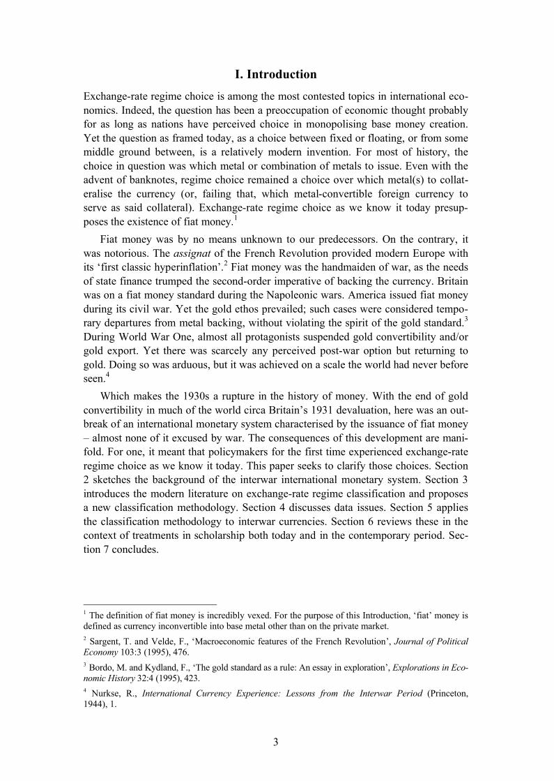
to gold. Large initial balances of foreign exchange and gold provided the cushion for this choice and for its ultimately unsatisfied waiting game. This was the ‘gold bloc’, whose most important member was France.9
Figure 1: Point of departure from the interwar gold standard
Source: Author’s dataset. See Part 4 for definitions of gold standard departure. Note: The y axis has no analytical significance.
But for most countries, the choice was immediate devaluation, often accompanied by trade barriers and sometimes capital controls, ranging from strenuous (Denmark) to informal (Britain). These were distinct from those applied in the exchange-clearing countries, evidence of which comes from Denmark. Its exchange controls initially provided the space to foment an accommodative domestic monetary policy and credit boom. Such breathing room was ephemeral: the authorities by 1935 were pressing hard on the brakes. Pressure to do so came precisely from the external accounts: Denmark had not insulated itself from international capital.
A peg to the pound had been established from 1 January 1933, at 20% below the 1929 value against sterling.10 The authorities held to this value as the boom in non-tradables inflated. The Economist noted in September 1934 that, ‘in certain quarters it is now believed that building activity is near the point at which the market for new
9 See Mour�, K., Managing the Franc Poincar�: Economic Understanding and Political Constraint in French Monetary Policy, 1928–1936 (Cambridge 1991).10 Sources for exchange rates are detailed in Section Four, as is the calculation of nominal- and real-effective exchange rates.
6
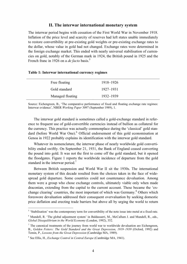
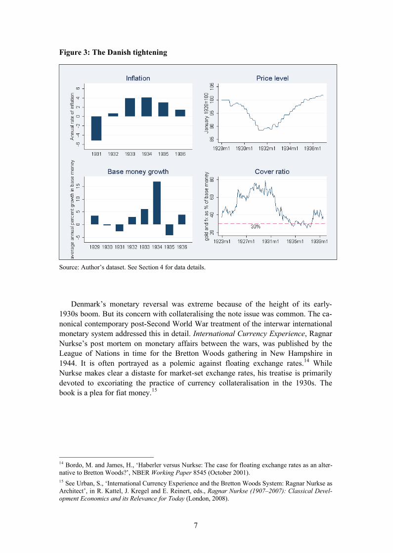
dwellings will be saturated.’11 Then, the authorities tightened. Base money growth switched from more than 20% in 1934 to –5% in 1935, a reversal greater than any to defend gold convertibility. It is hard to see inflation as the main concern; it peaked at 4% in 1934. Moreover, Danish policymakers, like most of this era, were concerned with the level of prices rather than the rate of change.12 By the end of 1934, the price level had only just regained its 1929 position.
Figure 2: Danish exchange rate
Source: Author’s dataset. See Part 4 for currency sources.
If prices mattered, it might have been in their contribution to sustainability of the currency regime. As in most of the countries that chose devaluation and mixed-strength capital controls, foreign reserves and gold were paramount. Their condition was reported in the financial press, soon after publication of regular central bank bal-ance sheet data (bank ‘returns’). Danish determination to stop the credit boom is lo-cated here. Foreign reserves and gold had fallen from 250 million kroner in 1931 to 150 million kroner in 1934. This was the amount of reserves which roughly covered a third of domestic sight liabilities, the minimum allowed by Danish statute.13
11 The Economist, ‘Economic Report (Denmark)’, 21 September 1934, 586. 12 Chadha, J., and Dimsdale, N., ‘A long view of real rates’, Oxford Review of Economic Policy 15:2 (1999), 17.13 International Currency Experience, 97.
7
Figure 3: The Danish tightening
Source: Author’s dataset. See Section 4 for data details.
Denmark’s monetary reversal was extreme because of the height of its early-1930s boom. But its concern with collateralising the note issue was common. The ca-nonical contemporary post-Second World War treatment of the interwar international monetary system addressed this in detail. International Currency Experience, Ragnar Nurkse’s post mortem on monetary affairs between the wars, was published by the League of Nations in time for the Bretton Woods gathering in New Hampshire in 1944. It is often portrayed as a polemic against floating exchange rates.14 While Nurkse makes clear a distaste for market-set exchange rates, his treatise is primarily devoted to excoriating the practice of currency collateralisation in the 1930s. The book is a plea for fiat money.15
14 Bordo, M. and James, H., ‘Haberler versus Nurkse: The case for floating exchange rates as an alter-native to Bretton Woods?’, NBER Working Paper 8545 (October 2001).15 See Urban, S., ‘International Currency Experience and the Bretton Woods System: Ragnar Nurkse as Architect’, in R. Kattel, J. Kregel and E. Reinert, eds., Ragnar Nurkse (1907–2007): Classical Devel-opment Economics and its Relevance for Today (London, 2008).
8
Regime choice in the 1930s
As the Danish example suggests, choice of the exchange-rate regime in the interwar period had implications for domestic policy independence and for the degree of eco-nomic integration with the rest of the world. This is a tradeoff familiar to policymak-ers today, and is framed as the macroeconomic policy trilemma. Also known as the ‘impossible trinity’, the trilemma is the medium-term impossibility of simultaneously enjoying free capital flows, a fixed-exchange rate and monetary policy independ-ence.16 On a larger scale, the trilemma offers a useful framework for characterising the international monetary system, a stylised version of which appears in Table 1. 17
Countries emerging from the First World War forewent exchange-rate fixity. After a period of floating, they stabilised on gold. To do so, they needed to foreswear inde-pendent policy.18 The 1931 rupture forced a new choice.
There is little in the literature to assess these choices on an empirical basis. More often, the period is used to associate outcomes with regime type, where regime type is taken a priori.19 This paper addresses that gap with a classification approach grounded in the methodology of the modern literature of de facto exchange rate re-gimes, to which we turn next.
16 Obstfeld, M., Shambaugh, J. and Taylor, A., ‘Monetary sovereignty, exchange rates, and capital con-trols: The trilemma in the interwar period,’ IMF Staff Papers 51 (2004).17 Harley, C.K., ‘Twentieth century monetary regimes in Canadian perspective’, working paper (2001).18 The inability of policymakers adequately to subvert domestic policy to the needs of the exchange rate is seen as the main cause of the circa-1931 worldwide breakdown of the gold standard; see Lessons From the Great Depression and Golden Fetters, op cit.19 See, for example, Eichengreen, B., ‘The comparative performance of fixed and floating exchange rate regimes: Interwar evidence’, NBER Working Paper 3097 (Sept 1989) and Bordo, M., ‘Exchange rate regime choice in historical perspective’, NBER Working Paper 9654 (April 2003)
9
III. Exchange-rate regime classificationThe Second Amendment to the IMF’s Articles of Agreement, in effect from 1978, deleted the provisions calling for maintenance of member currency parities into gold or the dollar, in a belated recognition of the collapse of the Bretton Woods system in 1971. The new articles merely enjoined countries to register regime type with the IMF and to ‘avoid manipulating exchange rates or the international monetary system in order to prevent effective balance of payments adjustment or to gain an unfair com-petitive advantage over other members…’.20
These self-registrations constituted a de jure classification of exchange-rate re-gime.21 A thread of economics literature has used these as a basis for ascertaining the importance of regime type for macroeconomic outcome (financial and real).22 Initial work concluded that exchange-rate regime matters little.23 Spurred in part by this sur-prising result, a de facto classification literature sprang up to infer from publicly available data whether de jure registrations were faithful to actual regime operation. This is the ‘Fear of floating’ literature, named for the eponymous 2000 paper by Calvo and Reinhart.24
At its core, exchange-rate-regime classification relies on measuring one or both of two observable statistics. The first is the exchange rate itself, which essentially meas-ures the outcome of the exchange-rate regime. This approach is not derived from the-ory but from stylised notions of regime type and exchange-rate outcome.25 A floating exchange-rate regime is presumed to be associated with a higher degree of exchange-rate variation vis-�-vis fixed regimes.26
The second observable statistic for regime classification is international reserves –a gauge of regime intention as opposed to regime outcome.27 The basis for this ap-proach is the balance-of-payments identity. Flows on capital and current account, mi-nus changes to international reserves, must net to zero (identity 1). Floating implies
20 International Monetary Fund, Articles of Agreement [revised] (Washington DC, 1977), Article IV, section 1, subsection (iii). 21 IMF de jure classifications are reported in International Monetary Fund, Annual Report on Exchange Arrangements and Exchange Restrictions (Washington DC, annual issues), beginning from 1950.22 The important early entry is Stockman, A. and Baxter, M., ‘Business cycles and the exchange-rate regime: Some international evidence’, Journal of Monetary Economics 23:3 (May 1989), 377–400. 23 The Stockman paper concludes, ‘We have been unable to find evidence that the cyclic behavior of real macroeconomic aggregates depends systematically on the exchange-rate regime.’ Ibid, 399. 24 Calvo, D. and Reinhart, C., ‘Fear of floating’, NBER Working Paper 7993 (November 2000). Subsequent footnotes refer to the journal article, Calvo, D. and Reinhart, C., ‘Fear of floating’, Quar-terly Journal of Economics 67:2 (May 2002), 379–408.25 According to some of the main contributors to the literature, most classification algorithms ‘do not correspond closely with theoretic concepts’. Ghosh, A., Gulde, A. and Wolf, H., Exchange Rate Re-gimes: Choices and Consequences (Cambridge MA, 2002), 43, footnote 3. 26 Methodologies based exclusively on the exchange rate include Reinhart, C. and Rogoff, K., ‘The modern history of exchange-rate arrangements: A reinterpretation’, NBER Working Paper 8963 (June 2002), 54–104 and Klein, M. and Shambaugh, J., ‘Fixed exchange rates and trade,’ Journal of Interna-tional Economics 70:2 (December 2006), p 359–383. 27 An additional instrument is the policy interest rate. This is rarely used in the literature. An exception is the exchange rate flexibility index developed by Calvo and Reinhart. ‘Fear of floating’, 402.
10
that current account imbalances are met on the capital account, with the exchange rate playing the equilibrating role (identity 2). By definition, international reserve balances are unchanged (identity 3).28
BoP identity CA + KA – ΔR ≡ 0 (1)
BoP identity, floating CA ≡ KA (2)
Floating condition Δ R = 0 (3)Appendix 1 reports the results of an application of these methodologies to modern
data. It finds that variation of the exchange rate is a poor guide to regime type. First, it overlooks the possibility that a credible floating regime can exhibit extremely low variability. Yet this is entirely possible, since agents in such a market have an incen-tive to trade in pro-stabilising directions. The practical consequence for the classifica-tion methodology is that floating regimes are often identified as heavily managed or even pegged. Thus Reinhart and Rogoff classify the UK (9/1992–12/2001) as ‘Man-aged floating’ but Australia (12/1983–12/2001) as ‘Freely floating’. The Swiss franc and Canadian dollar are ‘De facto moving bands’, while Japan is ‘Freely floating’(1/1977–12/2001). 29 The second problem with variation in the exchange rate is mis-identification of brittle pegs as floats. In other words, a heavily managed regime that periodically succumbs to devaluation pressure will exhibit a high variance statistic.
Appendix 1 reports that variance in international reserves also suffers from pit-falls. Reserve changes accruing from intervention must be ‘backed out’ from valua-tion effects; and this requires knowledge of reserves portfolio currency composition. In addition, reserves data are subject to misreporting and obfuscation; and in many cases are not available in high quality or requisite granularity.
Kurtosis
This paper proposes a new exchange-rate regime classification methodology based on kurtosis of the first derivative of the exchange rate with respect to time. It is an index of exchange-rate regime flexibility, based on the data-generating process underlying an exchange-rate time series. The hypothesis is that the degree of exchange-market intervention is revealed in a particular property of that series, namely the distribution of its changes. The intuition can be sketched with an historical example.
The classical gold standard ended with World War One. Thereafter, the ability to subvert domestic conditions to the needs of external balance consistent with a fixed
28 Methodologies using international reserves include ‘Fear of floating’ and Poirson, H., ‘How do coun-tries choose their exchange rate regime?’ IMF Working Paper 01/46 (April 2001). A third approach to classification is cluster analysis. This categorises regimes into five groups defined by least Euclidean distance from five cluster means of three variables: exchange-rate variation, reserves variation, and variation in the change of the exchange rate. See Levy-Yeyati, E. and Sturzenegger, F., ‘Classifying exchange rate regimes: Deeds vs. words’, European Economic Review 49:6 (August 2005), 1603–1635.29 Reinhart, C. and Rogoff, K., ‘The modern history of exchange rate arrangements: A reinterpretation’, NBER Working Paper 8963. The classifications appear on pages 56–102.
11
currency and open capital account was sharply reduced. This was partly the result of greater labour enfranchisement after the war. Eichengreen refers to this as the begin-ning of embedded liberalism, John Ruggie’s term for the state-society compact em-bedding macro-stabilisation policies within a larger market-based international sys-tem.30 Monetary authorities nevertheless continued to seek a ‘stable’ or fixed ex-change rate. This posed a dilemma because they could not rely on internal price flexi-bility to deliver balance-of-payments equilibrium. Yet they would not condone the use of the exchange rate to do so. The only equilibrating mechanism would be reserves –which were, by definition, a diminishing option under conditions of currency over-valuation. Here again is the trilemma. Nurkse commented on its interwar presence, noting that if the monetary authority chooses to peg, there is
no doubt [that] the maintenance of stable exchanges by [this] method presupposes an appropriate domestic credit policy.31
In the twentieth century beyond World War One, policymakers were expected both to deliver a ‘stable’ currency and a stable or indeed rising domestic price level, in most cases without the benefit of truly binding exchange controls.
Such conflict between external and internal goals produces a characteristic pattern of exchange-rate time series. Extended periods of extremely low exchange-rate vari-ability are punctuated by discrete, one-time changes. This happens because the peg cannot be held under a prolonged deficit in the external accounts. The resulting high variance statistic constitutes not floating but changes in de facto peg parities.32 This behaviour in the time series produces a unique shape in the distribution of percentage changes in the exchange rate, which can be used to detect regime type.
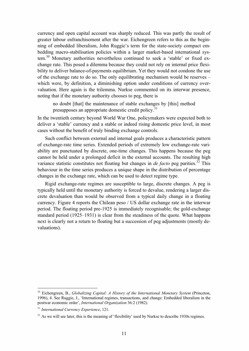
Rigid exchange-rate regimes are susceptible to large, discrete changes. A peg is typically held until the monetary authority is forced to devalue, rendering a larger dis-crete devaluation than would be observed from a typical daily change in a floating currency. Figure 4 reports the Chilean peso / US dollar exchange rate in the interwar period. The floating period pre-1925 is immediately recognisable; the gold-exchange standard period (1925–1931) is clear from the steadiness of the quote. What happens next is clearly not a return to floating but a succession of peg adjustments (mostly de-valuations).
30 Eichengreen, B., Globalizing Capital: A History of the International Monetary System (Princeton, 1996), 4. See Ruggie, J., ‘International regimes, transactions, and change: Embedded liberalism in the postwar economic order’, International Organization 36:2 (1982).31 International Currency Experience, 121. 32 As we will see later, this is the meaning of ‘flexibility’ used by Nurkse to describe 1930s regimes.
12
0.1
.2.3
0.1
.2.3
-50 0 50 100
-50 0 50 100
1919-1924 1925-1931
1932-1939Den
sity
weekly % change in exchange rate, usd numeraire
Figure 4: Chile peso / US dollar 1919–1940
Source: See ‘Data’ section in text. Notes: The vertical lines correspond with sterling’s September 1931 devaluation and the US dollar’s April 1933 devaluation.
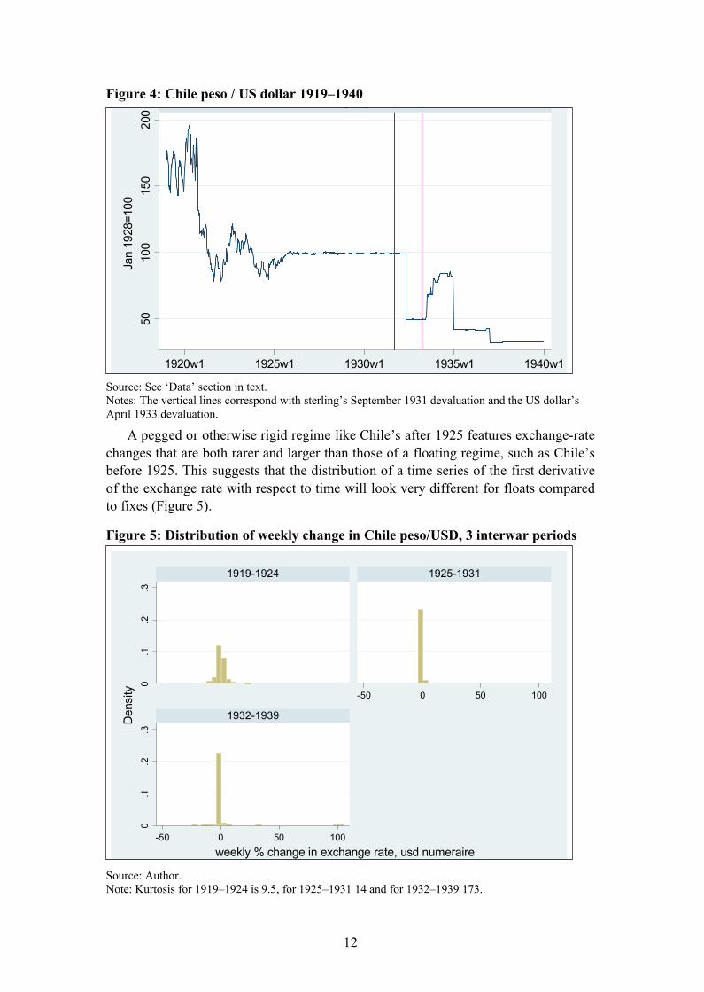
A pegged or otherwise rigid regime like Chile’s after 1925 features exchange-rate changes that are both rarer and larger than those of a floating regime, such as Chile’s before 1925. This suggests that the distribution of a time series of the first derivative of the exchange rate with respect to time will look very different for floats compared to fixes (Figure 5).
Figure 5: Distribution of weekly change in Chile peso/USD, 3 interwar periods
Source: Author. Note: Kurtosis for 1919–1924 is 9.5, for 1925–1931 14 and for 1932–1939 173.
5010
015
020
0
1920w1 1925w1 1930w1 1935w1 1940w1
Chile
Jan
1928
=100
13
05
-2 0 2 4 -2 0 2 4
Canada HK
Den
sity
weekly % change in exchange rateGraphs by country
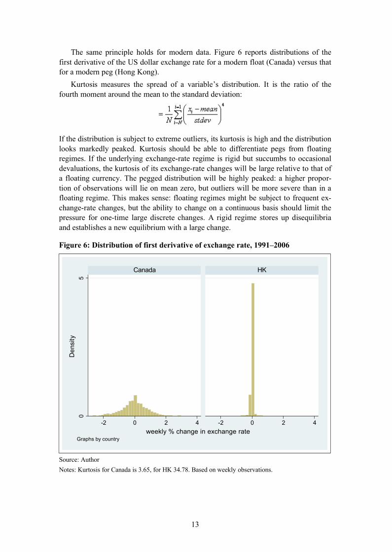
The same principle holds for modern data. Figure 6 reports distributions of the first derivative of the US dollar exchange rate for a modern float (Canada) versus that for a modern peg (Hong Kong).
Kurtosis measures the spread of a variable’s distribution. It is the ratio of the fourth moment around the mean to the standard deviation:
If the distribution is subject to extreme outliers, its kurtosis is high and the distribution looks markedly peaked. Kurtosis should be able to differentiate pegs from floating regimes. If the underlying exchange-rate regime is rigid but succumbs to occasional devaluations, the kurtosis of its exchange-rate changes will be large relative to that of a floating currency. The pegged distribution will be highly peaked: a higher propor-tion of observations will lie on mean zero, but outliers will be more severe than in a floating regime. This makes sense: floating regimes might be subject to frequent ex-change-rate changes, but the ability to change on a continuous basis should limit the pressure for one-time large discrete changes. A rigid regime stores up disequilibria and establishes a new equilibrium with a large change.
Figure 6: Distribution of first derivative of exchange rate, 1991–2006
Source: AuthorNotes: Kurtosis for Canada is 3.65, for HK 34.78. Based on weekly observations.
14
Kurtosis does not feature in the modern literature of exchange-rate regime classifica-tion. Eichengreen reports kurtosis of the exchange rate in levels (not in changes), and does not use it to assess regime type.33
Lamda-kurtosis index
Appendix 3 reviews the results of an application of kurtosis to the classification of exchange-rate regimes, with the same countries, samples and standards used to judge the performance of conventional methodologies. In this paper, a kurtosis-based index is used in which kurtosis of the first derivative of the exchange rate with respect to time is used to ‘scale’ the coefficient of variation of the exchange rate in levels:
Lamda-kurtosis index:
Coefficient of variation in the numerator is necessary to identify credible pegs. A credibly pegged regime might enjoy a ‘target zone’ distribution of exchange-rate changes, to the extent that markets anticipate the requisite actions by the authorities, and thus move the exchange rate into the target zone in a pro-stabilising way.34 The resulting distribution of changes is distinctly bi-modal. The kurtosis of such a distri-bution is lower than that of a normal distribution, and hence kurtosis alone would mis-identify such a credibly pegged regime as a float. Taking the square root of coefficient of variation reduces the power of large variation to overwhelm a large kurtosis statis-tic and produce a misleading index score.
Part 5 reports values of this index for stylised modern fixed and floating regimes, which can be used as a benchmark for assessing interwar regimes.
Numeraire issuesFlexibility indices incorporating a measure of the exchange rate (be it variation of the rate itself or kurtosis of its first derivative) will only be instructive if measuring the exchange rate vis-�-vis the proper reference currency, or ‘numeraire’. In other words, if the monetary authority is targeting the value of the currency expressed in euros, it makes no sense to apply a classification system to the a time-series of the exchange rate expressed in dollars. In the modern period, this is relatively straightforward. To the extent that a currency is managed, it is usually managed against the US dollar. The exceptions in the present paper are the CFA franc, Danish krone and Swedish krona,
33 Eichengreen, B., ‘The comparative performance of fixed and floating exchange rate regimes: Inter-war evidence’, NBER Working Paper 3097 (September 1989)34 With appreciation to Rui Pedro Esteves.
15
which are pegged against the euro, having previously been pegged against the French franc and German mark, respectively.35
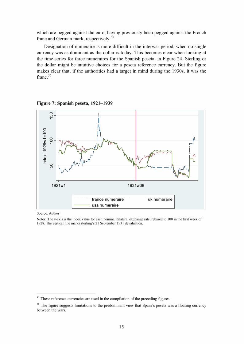
Designation of numeraire is more difficult in the interwar period, when no single currency was as dominant as the dollar is today. This becomes clear when looking at the time-series for three numeraires for the Spanish peseta, in Figure 24. Sterling or the dollar might be intuitive choices for a peseta reference currency. But the figure makes clear that, if the authorities had a target in mind during the 1930s, it was the franc.36
Figure 7: Spanish peseta, 1921–1939
Source: AuthorNotes: The y-axis is the index value for each nominal bilateral exchange rate, rebased to 100 in the first week of 1928. The vertical line marks sterling’s 21 September 1931 devaluation.
35 These reference currencies are used in the compilation of the preceding figures.36 The figure suggests limitations to the predominant view that Spain’s peseta was a floating currency between the wars.
5010
015
0
1921w1 1931w38
france numeraire uk numeraireusa numeraire
inde
x,19
28w
1=10
0
16
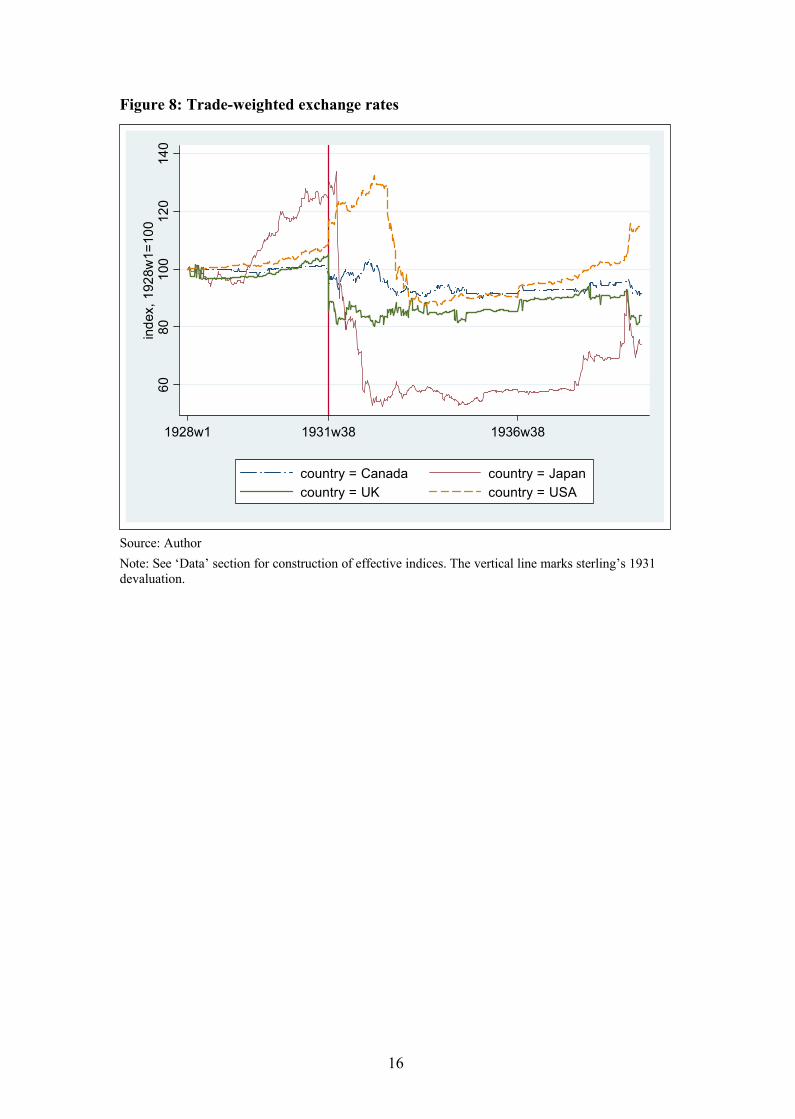
Figure 8: Trade-weighted exchange rates
Source: AuthorNote: See ‘Data’ section for construction of effective indices. The vertical line marks sterling’s 1931 devaluation.
6080
100
120
140
inde
x,19
28w
1=10
0
1928w1 1931w38 1936w38
country = Canada country = Japancountry = UK country = USA
17
IV. DataExchange rates
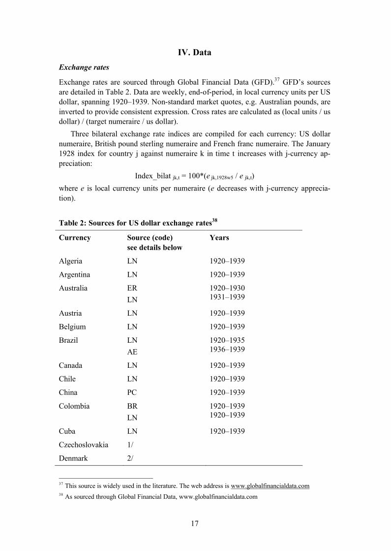
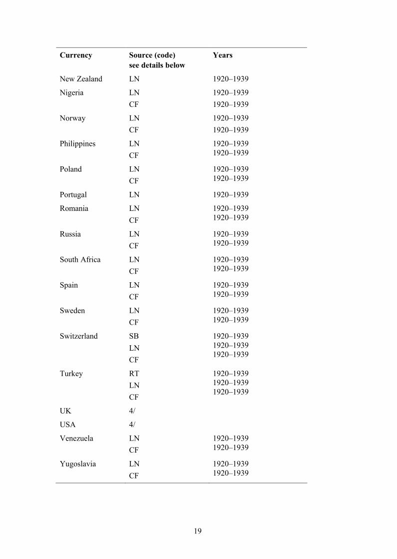
Exchange rates are sourced through Global Financial Data (GFD).37 GFD’s sources are detailed in Table 2. Data are weekly, end-of-period, in local currency units per US dollar, spanning 1920–1939. Non-standard market quotes, e.g. Australian pounds, are inverted to provide consistent expression. Cross rates are calculated as (local units / us dollar) / (target numeraire / us dollar).
Three bilateral exchange rate indices are compiled for each currency: US dollar numeraire, British pound sterling numeraire and French franc numeraire. The January 1928 index for country j against numeraire k in time t increases with j-currency ap-preciation:
Index_bilat jk,t = 100*(e jk,1928w5 / e jk,t)where e is local currency units per numeraire (e decreases with j-currency apprecia-tion).
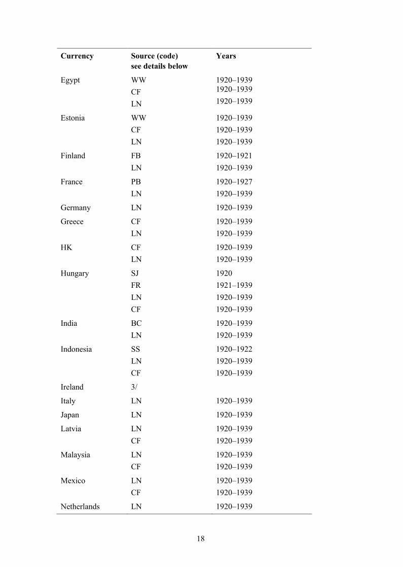
Table 2: Sources for US dollar exchange rates38
Currency Source (code) see details below
Years
Algeria LN 1920–1939
Argentina LN 1920–1939
Australia ERLN
1920–19301931–1939
Austria LN 1920–1939
Belgium LN 1920–1939
Brazil LNAE
1920–19351936–1939
Canada LN 1920–1939
Chile LN 1920–1939
China PC 1920–1939
Colombia BRLN
1920–19391920–1939
Cuba LN 1920–1939
Czechoslovakia 1/
Denmark 2/
37 This source is widely used in the literature. The web address is www.globalfinancialdata.com38 As sourced through Global Financial Data, www.globalfinancialdata.com
18
Currency Source (code) see details below
Years
Egypt WWCFLN
1920–19391920–19391920–1939
Estonia WWCFLN
1920–19391920–19391920–1939
Finland FBLN
1920–19211920–1939
France PBLN
1920–19271920–1939
Germany LN 1920–1939
Greece CFLN
1920–19391920–1939
HK CFLN
1920–19391920–1939
Hungary SJFRLNCF
19201921–19391920–19391920–1939
India BCLN
1920–19391920–1939
Indonesia SSLNCF
1920–19221920–19391920–1939
Ireland 3/
Italy LN 1920–1939
Japan LN 1920–1939
Latvia LNCF
1920–19391920–1939
Malaysia LNCF
1920–19391920–1939
Mexico LNCF
1920–19391920–1939
Netherlands LN 1920–1939
19
Currency Source (code) see details below
Years
New Zealand LN 1920–1939
Nigeria LNCF
1920–19391920–1939
Norway LNCF
1920–19391920–1939
Philippines LNCF
1920–19391920–1939
Poland LNCF
1920–19391920–1939
Portugal LN 1920–1939
Romania LNCF
1920–19391920–1939
Russia LNCF
1920–19391920–1939
South Africa LNCF
1920–19391920–1939
Spain LNCF
1920–19391920–1939
Sweden LNCF
1920–19391920–1939
Switzerland SBLNCF
1920–19391920–19391920–1939
Turkey RTLNCF
1920–19391920–19391920–1939
UK 4/
USA 4/
Venezuela LNCF
1920–19391920–1939
Yugoslavia LNCF
1920–19391920–1939
20
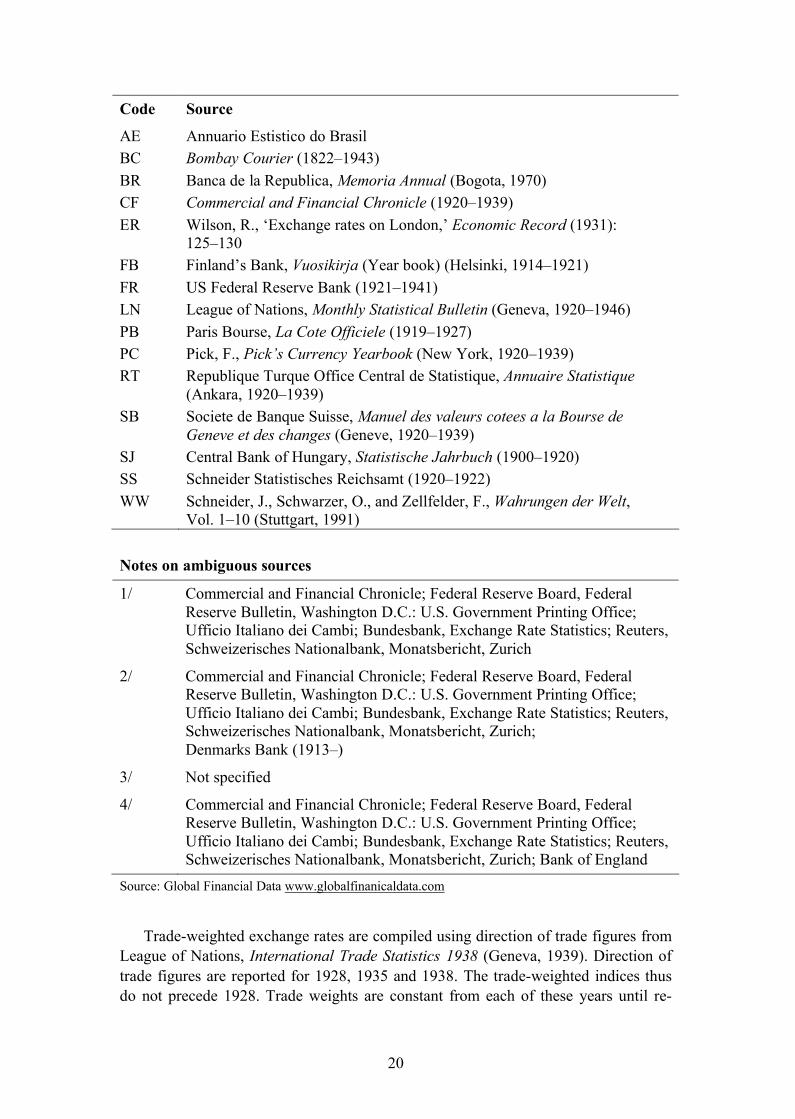
Code Source
AE Annuario Estistico do Brasil BC Bombay Courier (1822–1943)BR Banca de la Republica, Memoria Annual (Bogota, 1970) CF Commercial and Financial Chronicle (1920–1939)ER Wilson, R., ‘Exchange rates on London,’ Economic Record (1931):
125–130FB Finland’s Bank, Vuosikirja (Year book) (Helsinki, 1914–1921)FR US Federal Reserve Bank (1921–1941)LN League of Nations, Monthly Statistical Bulletin (Geneva, 1920–1946)PB Paris Bourse, La Cote Officiele (1919–1927)PC Pick, F., Pick’s Currency Yearbook (New York, 1920–1939)RT Republique Turque Office Central de Statistique, Annuaire Statistique
(Ankara, 1920–1939)SB Societe de Banque Suisse, Manuel des valeurs cotees a la Bourse de
Geneve et des changes (Geneve, 1920–1939)SJ Central Bank of Hungary, Statistische Jahrbuch (1900–1920)SS Schneider Statistisches Reichsamt (1920–1922)WW Schneider, J., Schwarzer, O., and Zellfelder, F., Wahrungen der Welt,
Vol. 1–10 (Stuttgart, 1991)
Notes on ambiguous sources
1/ Commercial and Financial Chronicle; Federal Reserve Board, Federal Reserve Bulletin, Washington D.C.: U.S. Government Printing Office; Ufficio Italiano dei Cambi; Bundesbank, Exchange Rate Statistics; Reuters, Schweizerisches Nationalbank, Monatsbericht, Zurich
2/ Commercial and Financial Chronicle; Federal Reserve Board, Federal Reserve Bulletin, Washington D.C.: U.S. Government Printing Office; Ufficio Italiano dei Cambi; Bundesbank, Exchange Rate Statistics; Reuters, Schweizerisches Nationalbank, Monatsbericht, Zurich; Denmarks Bank (1913–)
3/ Not specified
4/ Commercial and Financial Chronicle; Federal Reserve Board, Federal Reserve Bulletin, Washington D.C.: U.S. Government Printing Office; Ufficio Italiano dei Cambi; Bundesbank, Exchange Rate Statistics; Reuters, Schweizerisches Nationalbank, Monatsbericht, Zurich; Bank of England
Source: Global Financial Data www.globalfinanicaldata.com
Trade-weighted exchange rates are compiled using direction of trade figures from League of Nations, International Trade Statistics 1938 (Geneva, 1939). Direction of trade figures are reported for 1928, 1935 and 1938. The trade-weighted indices thus do not precede 1928. Trade weights are constant from each of these years until re-
21
placed by the succeeding years. For example, the weight of the UK in Argentine trade in December 1934 is the 1928 weight.
These weights are usefully located, respectively, inside of the interwar gold stan-dard (1925–1931), and before and after the Tripartite Agreement (September 1936). The trade weight is the proportion of trading partner trade in total home country ex-ports and imports in goods. Effective indices are geometric averages of individual weighted percent weekly changes in cross rates. For a given country, the index is:
where wi is the proportion of total trade conducted with partner i and e is percent weekly change in the bilateral cross-rate with the currency of partner k, where the cross-rate is quoted in local currency units per partner currency.
Numeraire
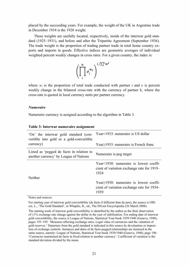
Numeraire currency is assigned according to the algorithm in Table 3.
Table 3: Interwar numeraire assignment
‘On’ the interwar gold standard (con-vertible into gold or a gold-convertible currency)
Year<1933: numeraire is US dollar
Year≥1933: numeraire is French franc
Listed as ‘pegged de facto in relation to another currency’ by League of Nations Numeraire is peg target
Neither
Year<1930: numeraire is lowest coeffi-cient of variation exchange rate for 1919–1924
Year≥1930: numeraire is lowest coeffi-cient of variation exchange rate for 1934–1939
Notes and sources: For starting year of interwar gold convertibility (de facto if different than de jure), the source is Offi-cer, L., ‘The Gold Standard’, in Whaples, R., ed., The EH.net Encyclopedia (26 March 2008). The starting week of interwar gold convertibility is identified by the author as the final observation of ≥1% exchange rate change against the dollar in the year of stabilisation. For ending date of interwar gold convertibility, the source is League of Nations, Statistical Year-book 1939/1940 (Geneva, 1940), pages 193–195: ‘Measures affecting exchange rates, Legal value of currencies and the valuation of gold reserves.’ Departure from the gold standard is indicated in this source by devaluation or imposi-tion of exchange controls. Instances and dates of de facto pegged relationships are itemised in thesame source, namely: League of Nations, Statistical Year-book 1939/1940 (Geneva, 1940), page 196: ‘Currencies maintained de facto in fixed relation to another currency’. Coefficient of variation is the standard deviation divided by the mean.
22
It is customary to see the dollar as the only reference currency for the immediate post-World War One period, since only it was stabilised on gold. This was certainly the opinion of some contemporary observers,39 but it might not reflect those of poli-cymakers. It may be that currencies, to the extent that they were guided, were done so with reference to the most important trade partner. As such, numeraire assignment here follows lowest coefficient of variation of the exchange rate, assigned separately for the pre- and post-1931 period. In the first, it is based on 1919–1924; and the sec-ond is 1934–1939. However, numeraire assignment is automatic (a) where the cur-rency is on the gold standard, in which case the numeraire is the US dollar pre 1933 and France thereafter, and (b) where the currency is listed by the League of Nations as ‘fixed in relation de facto to another currency.40
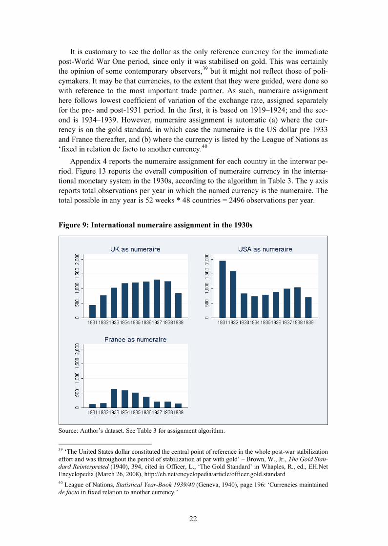
Appendix 4 reports the numeraire assignment for each country in the interwar pe-riod. Figure 13 reports the overall composition of numeraire currency in the interna-tional monetary system in the 1930s, according to the algorithm in Table 3. The y axis reports total observations per year in which the named currency is the numeraire. The total possible in any year is 52 weeks * 48 countries = 2496 observations per year.
Figure 9: International numeraire assignment in the 1930s
Source: Author’s dataset. See Table 3 for assignment algorithm.
39 ‘The United States dollar constituted the central point of reference in the whole post-war stabilization effort and was throughout the period of stabilization at par with gold’ – Brown, W., Jr., The Gold Stan-dard Reinterpreted (1940), 394, cited in Officer, L., ‘The Gold Standard’ in Whaples, R., ed., EH.Net Encyclopedia (March 26, 2008), http://eh.net/encyclopedia/article/officer.gold.standard 40 League of Nations, Statistical Year-Book 1939/40 (Geneva, 1940), page 196: ‘Currencies maintained de facto in fixed relation to another currency.’
23
Analytic weights
For summary statistics, analytic weights are share of panel GDP in constant dollars. The source is Maddison, A., ‘Historical Statistics for the World Economy: 1–2006 AD’, Excel dataset, 2008. Gaps are imputed from time trends; missing observations are estimated from historic ratios to world GDP. For the modern (post-WW2) period, analytic weights are share of panel exports of goods, from International Monetary Fund, International Financial Statistics.
Dynamic index for classification methodologies
For each country in the panel, a ‘dynamic numeraire’ bilateral index is compiled in which the index value for time t is the index value in t–1 multiplied by the proportion-ate change in the numeraire exchange rate between time t–1 and time t. This allows changes of currency peg target to be made without disturbing the time series.
‘Lunar’ year
Insofar as the classification algorithms are reported on an annual basis (i.e. country X in year Y), there is a distinct possibility of missing important monetary changes intro-duced on the first day or week of the year. Thus the annual flexibility indices measure the current year plus the last observation of the previous year. For example, coeffi-cient of variation of the exchange rate for 1933 is calculated over a period beginning in week 52 of 1932 and ending in week 52 of 1933; the coefficient of reserves is cal-culated similarly, over a 13-month year.
Reserves and sight liabilities
Foreign exchange and gold reserves data, as well as those for sight liabilities of the monetary authority, are from three sources. First is the US Federal Reserve, Bulletin(Washington DC, various issues), published monthly. Second is League of Nations, Monthly Statistical Bulletin (Geneva, various issues). Third is The Economist (Lon-don, various issues). All are transcribed by the author and checked for data entry er-rors. Figures are monthly, in millions of local currency units. Gold is valued at the latest legal parity and foreign exchange reserves are valued at market exchange rates.41
These are reserves of the central bank or monetary authority. However, in this pe-riod, several countries created specialised currency-intervention funds with the pro-ceeds from gold revaluation. The first intervention fund was Britain’s Exchange
41 The League of Nations Bulletin remarks in a footnote that ‘foreign reserves are believed to be valued at current exchange rates’ and that gold is valued at the latest legal parity. Ideally, foreign-currency values of these reserves should be backed out of the local currency figures. This approach is not fol-lowed in the present draft. However, for the reader’s benefit, international reserve series are reported in the appendix for four different numeraires: local currency, the French franc, the British pound, and the US dollar.
24
Equalisation Account (EEA), set up in 1932.42 This was joined by the United States (1934), Belgium (1935), and Switzerland, France and Holland (1936). Funds of less importance were set up in Canada and Argentina (1935); Spain, Latvia and Czecho-slovakia (1936); Colombia and Japan (1937); and China (1939).43
The author is aware of assets data only for the British EEA with monthly fre-quency. Unfortunately, even this source covers only discontinuous parts of the 1932–1939 period, making it of limited use in classification work.
For the modern period, reserves are reported in US dollars and re-denominated bythe author where the country has an explicit or widely recognised non-US peg target. This means the Euro for EMR2 members and, for pre-1999, the Deutsche mark for ERM1/EMS members, and France for the CFA franc.
Panel and period
The broad panel contains 48 currencies, for which full exchange rate data are avail-able and all cross rates are calculated, mostly in weekly observations from 1919 to 1939. Of these, 30 members, representing the preponderance of world trade, also have reserves data, for 1923–1939. Observations for 1939 are truncated in order to exclude the outbreak of World War II: they run January-August inclusive (weeks 1 through 35). Statistics reported for 1939 are for this shortened time-span.
Gold convertibility, fx convertibility, and peg status
The interwar dataset is coded for observance of the gold standard. An observation is marked gold-convertible (i.e. on the gold standard) if it accords with Officer 2008. Officer reports only years of observance. 44 For weekly granularity, the gold standard is coded within the year reported by Officer, beginning with the final observation of 1% or greater change in the exchange rate against the dollar. The precise ending date of the gold standard is taken from League of Nations, Statistical Year-book 1933/1934(Geneva, 1934), page 206: ‘Dates of principal measures affecting exchange rates’. For later in the decade, the source is League of Nations, Statistical Year-book 1939/1940 (Geneva, 1940), pages 193–195: ‘Measures affecting exchange rates, legal value of currencies and the valuation of gold reserves.’ The Yearbook lists devaluations and capital controls separately from ‘Suspension’ of the gold standard. In the author’s dataset, convertibility is marked zero with the first of any violation of the gold-standard ethos (devaluation, fx controls or convertibility suspension). Foreign exchange convertibility in the 1930s is coded 0/1 in accordance with League of Nations, Statistical Year-Book 1939/40 (Geneva, 1940), pages 193–195: ‘Measures affecting exchange rates, Legal value of currencies and the valuation of gold re-serves.’ Peg status (for the purpose of nomination of numeraire currency), is taken
42 Incomplete EEA data are reported by Howson for parts of 1932–1939. Howson, S., Sterling’s Man-aged Float: The Operations of the Exchange Equalisation Account, 1932–39 (Princeton, 1980).43 Bloomfield, A., Capital Imports and the American Balance of Payments 1934–39: A Study in Ab-normal International Capital Transfers (Chicago, 1950), 148.44 Officer, L., ‘The Gold Standard’, in Whaples, R., ed., The EH.net Encyclopedia (2008)
25
from League of Nations, Statistical Year-Book 1939/40 (Geneva, 1940), page 196: ‘Currencies maintained de facto in fixed relation to another currency’ and from Nurkse (1944), page 51: The Sterling Area.
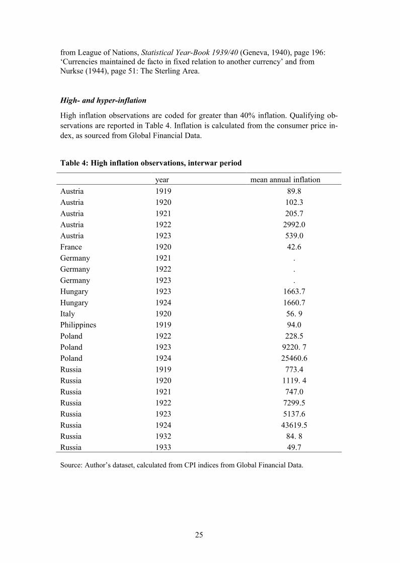
High- and hyper-inflation
High inflation observations are coded for greater than 40% inflation. Qualifying ob-servations are reported in Table 4. Inflation is calculated from the consumer price in-dex, as sourced from Global Financial Data.
Table 4: High inflation observations, interwar period
year mean annual inflationAustria 1919 89.8Austria 1920 102.3Austria 1921 205.7Austria 1922 2992.0Austria 1923 539.0France 1920 42.6Germany 1921 .Germany 1922 .Germany 1923 .Hungary 1923 1663.7Hungary 1924 1660.7Italy 1920 56. 9Philippines 1919 94.0Poland 1922 228.5Poland 1923 9220. 7Poland 1924 25460.6Russia 1919 773.4Russia 1920 1119. 4Russia 1921 747.0Russia 1922 7299.5Russia 1923 5137.6Russia 1924 43619.5Russia 1932 84. 8Russia 1933 49.7
Source: Author’s dataset, calculated from CPI indices from Global Financial Data.
26
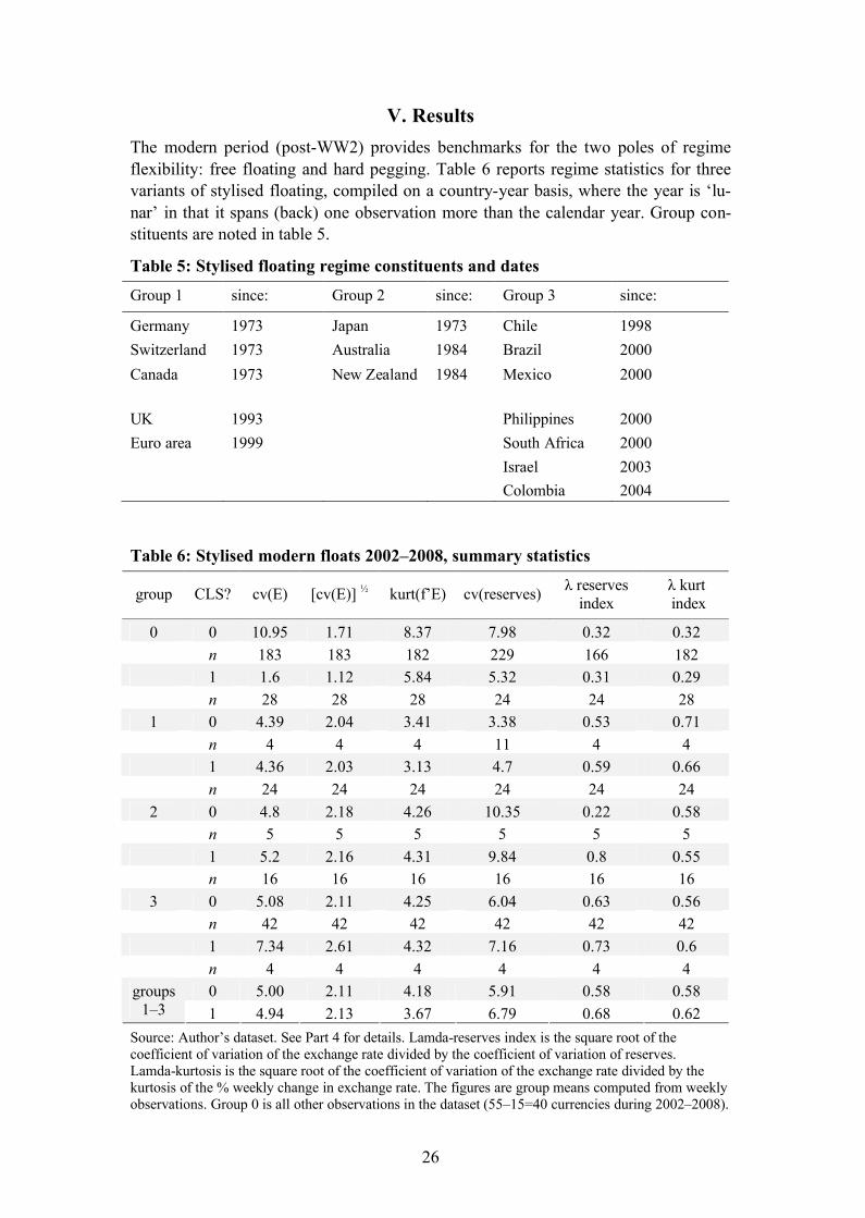
V. ResultsThe modern period (post-WW2) provides benchmarks for the two poles of regime flexibility: free floating and hard pegging. Table 6 reports regime statistics for three variants of stylised floating, compiled on a country-year basis, where the year is ‘lu-nar’ in that it spans (back) one observation more than the calendar year. Group con-stituents are noted in table 5.
Table 5: Stylised floating regime constituents and datesGroup 1 since: Group 2 since: Group 3 since:
Germany 1973 Japan 1973 Chile 1998Switzerland 1973 Australia 1984 Brazil 2000Canada 1973 New Zealand 1984 Mexico 2000
UK 1993 Philippines 2000Euro area 1999 South Africa 2000
Israel 2003Colombia 2004
Table 6: Stylised modern floats 2002–2008, summary statistics
group CLS? cv(E) [cv(E)] � kurt(f’E) cv(reserves) λ reserves index
λ kurtindex
0 0 10.95 1.71 8.37 7.98 0.32 0.32n 183 183 182 229 166 1821 1.6 1.12 5.84 5.32 0.31 0.29n 28 28 28 24 24 28
1 0 4.39 2.04 3.41 3.38 0.53 0.71n 4 4 4 11 4 41 4.36 2.03 3.13 4.7 0.59 0.66n 24 24 24 24 24 24
2 0 4.8 2.18 4.26 10.35 0.22 0.58n 5 5 5 5 5 51 5.2 2.16 4.31 9.84 0.8 0.55n 16 16 16 16 16 16
3 0 5.08 2.11 4.25 6.04 0.63 0.56n 42 42 42 42 42 421 7.34 2.61 4.32 7.16 0.73 0.6n 4 4 4 4 4 40 5.00 2.11 4.18 5.91 0.58 0.58groups
1–3 1 4.94 2.13 3.67 6.79 0.68 0.62Source: Author’s dataset. See Part 4 for details. Lamda-reserves index is the square root of the coefficient of variation of the exchange rate divided by the coefficient of variation of reserves. Lamda-kurtosis is the square root of the coefficient of variation of the exchange rate divided by the kurtosis of the % weekly change in exchange rate. The figures are group means computed from weekly observations. Group 0 is all other observations in the dataset (55–15=40 currencies during 2002–2008).
27
Does the kurtosis-based flexibility index merely reward market volume? In order to control for this possibility, Table 6 reports regime statistics segregated by trading in the Continuous Linked Settlement system.45
Table 7: Currencies traded through CLS
since: since:
Australia 2002m9 New Zealand 2004m12Canada 2002m9 Norway 2003m9Denmark 2003m9 Singapore 2003m9Euro area 2002m9 South Africa 2004m12Hong Kong 2004m12 South Korea 2004m12Israel 2008m5 Sweden 2003m9Japan 2002m9 Switzerland 2002m9Mexico 2008m5 United Kingdom 2002m9Source: CLS Bank.
Tables 8 and 9 are analogous to 5 and 6. Again, to control for market liquidity, pegs are grouped by CLS membership as per Table 7.
Table 8: Stylised pegs and dates
Group 5 Group 6Bretton Woods East Asia pegs
Group 4Modern pegs since:
1948–1970 1991–1996Latvia 2005m5 Denmark HKSlovakia 2005m12 Belgium IndonesiaEstonia 2004m7 Finland MalaysiaLithuania 2004m7 France KoreaSlovenia 2004m6 Germany TaiwanHK 1983m10 Greece ThailandDenmark 1979m3 Japan Singapore
NetherlandsSpainSwitzerlandUK
45 CLS can be thought of as an instrument for market liquidity. CLS Bank is owned by the world’s largest banks to manage settlement of foreign exchange between them (and for their customers and other third parties). CLS-traded currencies are listed in Table 6.
28
Table 9: Stylised pegs; groups defined in Table 8
group CLS? cv(E) [cv(E)] � kurt(f’E) cv(reserves) λ reserves index
λ kurt index
0 0 8.92 1.74 12.09 12.42 0.24 0.34n 2694 2694 2187 1853 1752 21870* 6.66 1.5 11.52 11.75 0.23 0.3n 2503 2503 2005 1721 1620 20051 4.33 1.98 3.77 6.88 0.62 0.56n 59 59 59 55 55 59
4 0 0.66 0.69 6.71 9.63 0.13 0.16n 57 57 57 48 48 571 0.5 0.62 7.86 3.72 0.24 0.15n 13 13 13 13 13 13
5 0 2.82 0.77 14.47 18.24 0.05 0.09n 264 264 197 147 147 197
6 0 1.23 1.03 7.15 7.68 0.17 0.23n 49 49 49 41 41 490 2.28 0.79 11.83 14.65 0.09 0.13Groups
4–6 1 0.50 0.62 7.86 3.72 0.24 0.15
Source: Author’s dataset. See Table 6 for detailed notes. * excludes ‘freely falling’ regimes, i.e. where inflation is greater than 40%.
Interwar period
Table 10: Interwar regime statistics, 1919–1939, by gold and fx convertibility
GS? FX? cv(E) [cv(E)] � kurt(f’E) cv (reserves)a
λ re-serves index a
λ reserves index b
λ kurt index
0 0 7.49 1.96 13.88 11.04 0.80 0.13 0.24
n 187 187 178 102 98 83 187
1 6.63 1.97 9.48 10.98 2.16 0.10 0.39
n 542 542 473 218 211 161 542
1 1 1.65 0.68 9.39 9.13 0.12 0.04 0.13
n 267 267 227 172 169 139 266
Source: Author’s dataset. ‘GS’ indicates convertibility under the interwar gold standard. ‘FX’ indicates foreign-exchange convertibility. Sources for both are detailed in Part 4. (a) Reserves of gold andforeign exchange. (b) Foreign-exchange reserves only. ‘n’ is the number of individual country-year
statistics making up the mean. Reserve statistics cover a subset of the panel dataset, as detailed in Part 4.
Table 10 reports the key interwar regime statistics for reserves- and kurtosis-based flexibility indices, grouped by gold-standard convertibility (‘GS?’) and foreign-
29
exchange convertibility (‘FX?’). In Table 11, the mean country-year statistic is grouped by phase of gold convertibility. Stage 1 is for all country-years prior to con-vertibility. For example, for Britain this is 1919–1924. Stage 2 is the beginning year of convertibility. Stage 3 is for country-years on convertibility. Stage 4 is the transi-tion year when convertibility is lost. Stage 5 is for years off convertibility. Table 12 breaks out high-inflation observations during stage 1. Table 13 reports regime statis-tics for stage 5 by status of foreign-exchange convertibility.
Table 11: International monetary system, 1919–39, by stage of gold convertibility
stage cv(E) [cv(E)] � kurt(f’E) cv (reserves)a
λ reserves index a
λ reserves index b
λ kurt index
1 10.55 2.51 6.96 11.13 6.09 0.19 0.53n 356 356 311 74 68 51 3562 7.01 2 12.47 13.69 1.49 0.06 0.31n 33 33 33 19 18 12 333 1.21 0.63 9.5 9.23 0.12 0.04 0.11n 263 263 223 173 170 140 2624 5.27 1.86 21.02 18.43 0.23 0.08 0.12n 42 42 39 28 28 23 425 3 1.37 13.15 9.65 0.44 0.10 0.18n 303 303 273 199 195 158 303
Sources and notes: Author’s dataset. See Part 4 for details. Phase 1 is for country-year statistics in years before convertibility. Phase 2 is in the year of transition to convertibility. Phase 3 is duringconvertibility. Phase 4 is in the transition year to post-convertibility. Phase 5 is post-convertibility.
(a) Reserves of gold and foreign exchange. (b) Foreign-exchange reserves only. ‘n’ is the number of individual country-year statistics making up the mean. Reserve statistics cover a subset of the panel, as detailed in Part 4.
Table 12: Interwar stage 1, by inflation category
40%+ inflation cv(E) [cv(E)]
� kurt(f’E) Cv(reserves)a
λ reserves index a
λ reserves index b
λ kurt index
0 7.55 2.24 6.88 11.17 6.18 0.19 0.49n 334 334 291 73 67 50 3341 56.07 6.6 8.05 7.93 0.27 0.27 1.24n 22 22 20 1 1 1 22
Source and notes: As in Table 10. The first row provides the regime statistics excluding observations with 40% or higher inflation, as reported in Table 4.
30
Table 13: Interwar stage 5, by fx convertibility
fx open cv(E) [cv(E)] � kurt(f’E) cv (reserves)a
λ reserves index a
λ reserves index b
λ kurt index
0 4.07 1.63 14.31 9.41 0.64 0.09 0.18n 139 139 135 89 85 70 139
btwnc 5.79 2.03 11.69 22.25 0.43 0.15 0.28n 8 8 8 7 7 5 81 1.91 1.1 12.03 9 0.28 0.10 0.17n 156 156 130 103 103 83 156
Sources and notes: As in Table 11. Note (c): Statistic for year of switch between open and closed fx regime.
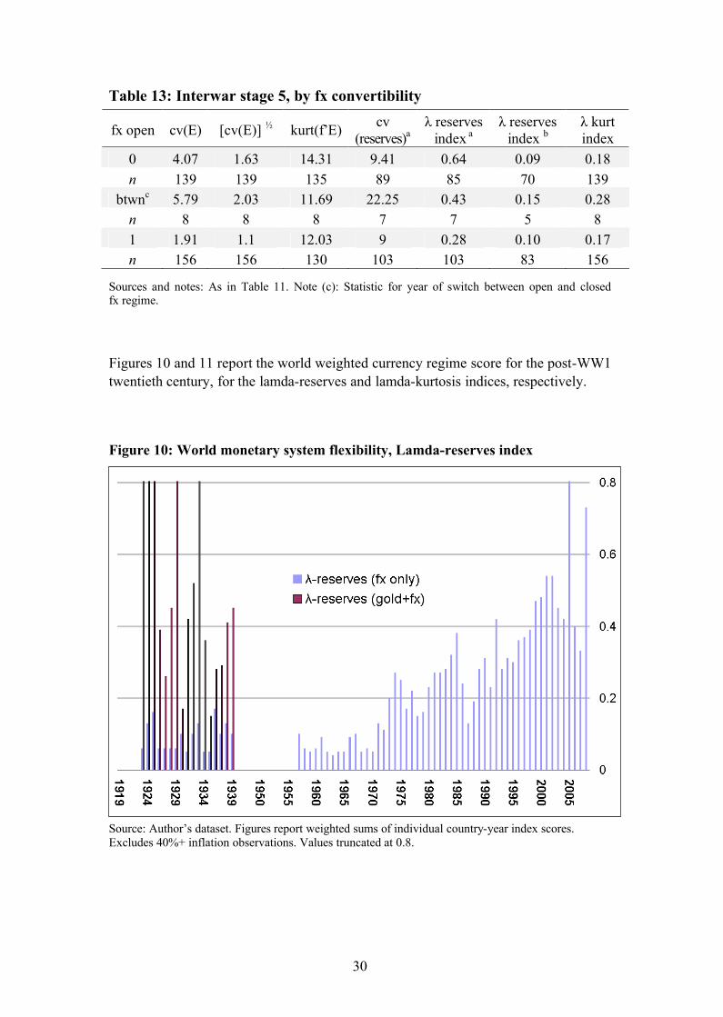
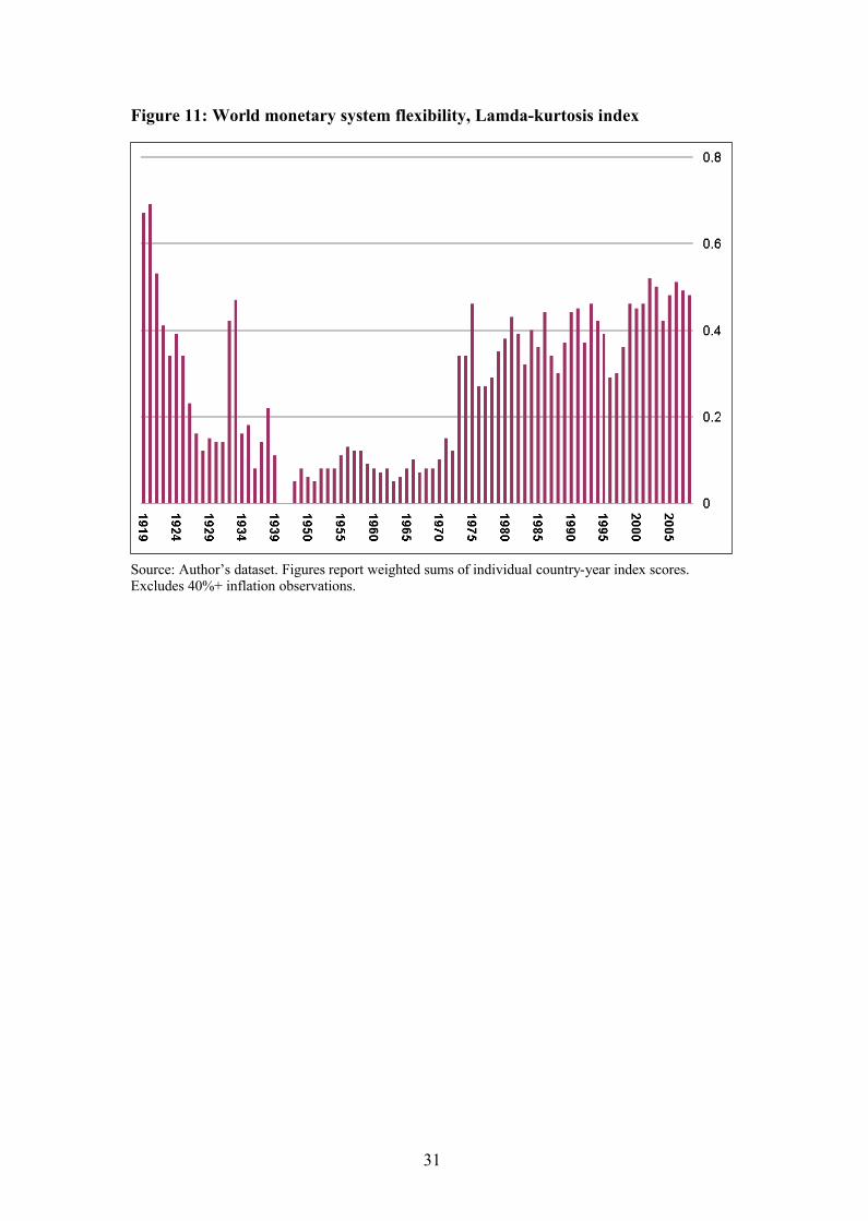
Figures 10 and 11 report the world weighted currency regime score for the post-WW1 twentieth century, for the lamda-reserves and lamda-kurtosis indices, respectively.
Figure 10: World monetary system flexibility, Lamda-reserves index
Source: Author’s dataset. Figures report weighted sums of individual country-year index scores. Excludes 40%+ inflation observations. Values truncated at 0.8.
31
Figure 11: World monetary system flexibility, Lamda-kurtosis index
Source: Author’s dataset. Figures report weighted sums of individual country-year index scores. Excludes 40%+ inflation observations.
32
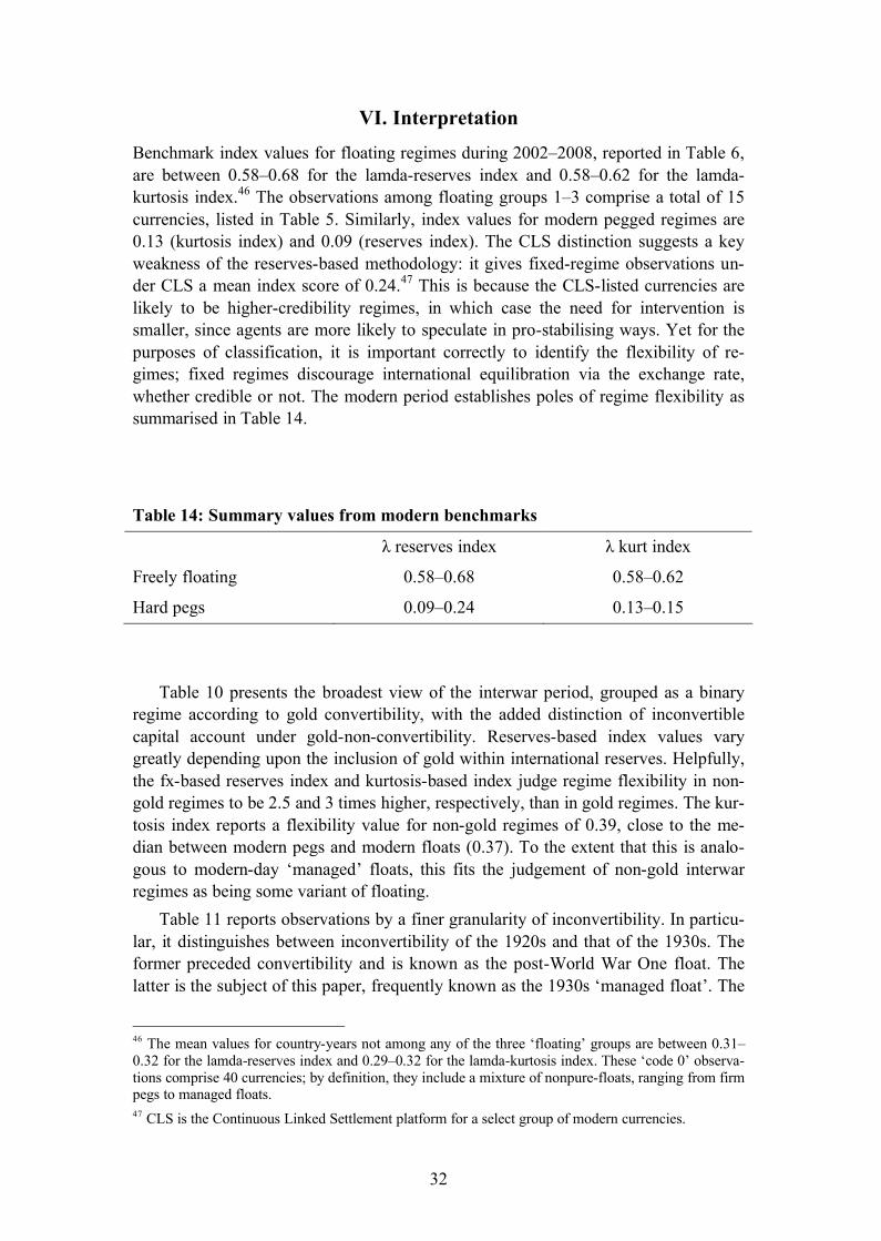
VI. InterpretationBenchmark index values for floating regimes during 2002–2008, reported in Table 6, are between 0.58–0.68 for the lamda-reserves index and 0.58–0.62 for the lamda-kurtosis index.46 The observations among floating groups 1–3 comprise a total of 15 currencies, listed in Table 5. Similarly, index values for modern pegged regimes are 0.13 (kurtosis index) and 0.09 (reserves index). The CLS distinction suggests a key weakness of the reserves-based methodology: it gives fixed-regime observations un-der CLS a mean index score of 0.24.47 This is because the CLS-listed currencies are likely to be higher-credibility regimes, in which case the need for intervention is smaller, since agents are more likely to speculate in pro-stabilising ways. Yet for the purposes of classification, it is important correctly to identify the flexibility of re-gimes; fixed regimes discourage international equilibration via the exchange rate, whether credible or not. The modern period establishes poles of regime flexibility as summarised in Table 14.
Table 14: Summary values from modern benchmarks
λ reserves index λ kurt index
Freely floating 0.58–0.68 0.58–0.62
Hard pegs 0.09–0.24 0.13–0.15
Table 10 presents the broadest view of the interwar period, grouped as a binary regime according to gold convertibility, with the added distinction of inconvertible capital account under gold-non-convertibility. Reserves-based index values vary greatly depending upon the inclusion of gold within international reserves. Helpfully, the fx-based reserves index and kurtosis-based index judge regime flexibility in non-gold regimes to be 2.5 and 3 times higher, respectively, than in gold regimes. The kur-tosis index reports a flexibility value for non-gold regimes of 0.39, close to the me-dian between modern pegs and modern floats (0.37). To the extent that this is analo-gous to modern-day ‘managed’ floats, this fits the judgement of non-gold interwar regimes as being some variant of floating.
Table 11 reports observations by a finer granularity of inconvertibility. In particu-lar, it distinguishes between inconvertibility of the 1920s and that of the 1930s. The former preceded convertibility and is known as the post-World War One float. The latter is the subject of this paper, frequently known as the 1930s ‘managed float’. The
46 The mean values for country-years not among any of the three ‘floating’ groups are between 0.31–0.32 for the lamda-reserves index and 0.29–0.32 for the lamda-kurtosis index. These ‘code 0’ observa-tions comprise 40 currencies; by definition, they include a mixture of nonpure-floats, ranging from firm pegs to managed floats.47 CLS is the Continuous Linked Settlement platform for a select group of modern currencies.
33
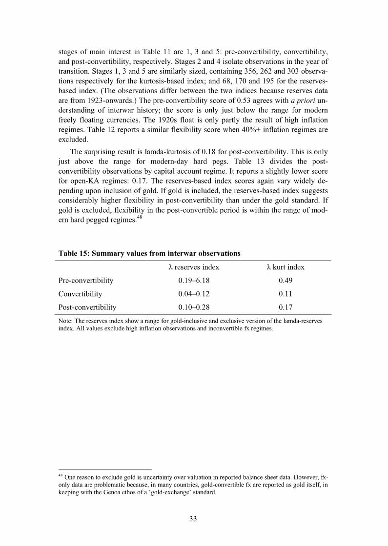
stages of main interest in Table 11 are 1, 3 and 5: pre-convertibility, convertibility, and post-convertibility, respectively. Stages 2 and 4 isolate observations in the year of transition. Stages 1, 3 and 5 are similarly sized, containing 356, 262 and 303 observa-tions respectively for the kurtosis-based index; and 68, 170 and 195 for the reserves-based index. (The observations differ between the two indices because reserves data are from 1923-onwards.) The pre-convertibility score of 0.53 agrees with a priori un-derstanding of interwar history; the score is only just below the range for modern freely floating currencies. The 1920s float is only partly the result of high inflation regimes. Table 12 reports a similar flexibility score when 40%+ inflation regimes areexcluded.
The surprising result is lamda-kurtosis of 0.18 for post-convertibility. This is only just above the range for modern-day hard pegs. Table 13 divides the post-convertibility observations by capital account regime. It reports a slightly lower score for open-KA regimes: 0.17. The reserves-based index scores again vary widely de-pending upon inclusion of gold. If gold is included, the reserves-based index suggests considerably higher flexibility in post-convertibility than under the gold standard. If gold is excluded, flexibility in the post-convertible period is within the range of mod-ern hard pegged regimes.48
Table 15: Summary values from interwar observations
λ reserves index λ kurt index
Pre-convertibility 0.19–6.18 0.49
Convertibility 0.04–0.12 0.11
Post-convertibility 0.10–0.28 0.17
Note: The reserves index show a range for gold-inclusive and exclusive version of the lamda-reserves index. All values exclude high inflation observations and inconvertible fx regimes.
48 One reason to exclude gold is uncertainty over valuation in reported balance sheet data. However, fx-only data are problematic because, in many countries, gold-convertible fx are reported as gold itself, in keeping with the Genoa ethos of a ‘gold-exchange’ standard.
34
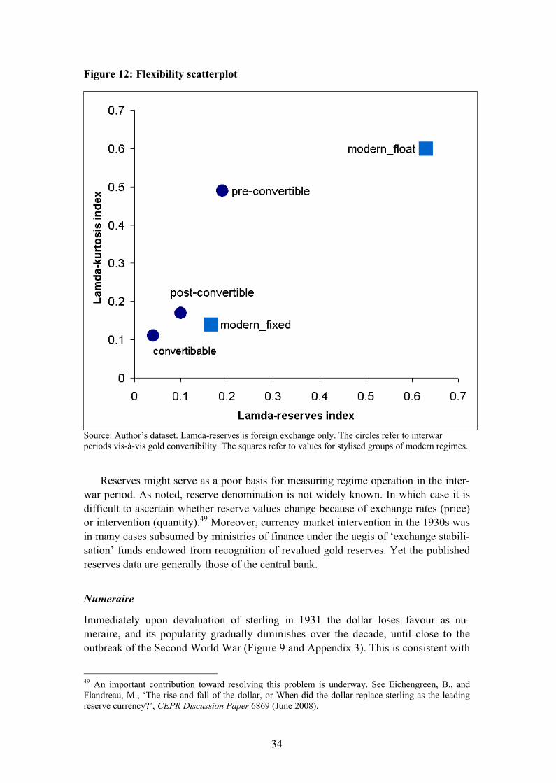
Figure 12: Flexibility scatterplot
Source: Author’s dataset. Lamda-reserves is foreign exchange only. The circles refer to interwar periods vis-�-vis gold convertibility. The squares refer to values for stylised groups of modern regimes.
Reserves might serve as a poor basis for measuring regime operation in the inter-war period. As noted, reserve denomination is not widely known. In which case it is difficult to ascertain whether reserve values change because of exchange rates (price) or intervention (quantity).49 Moreover, currency market intervention in the 1930s was in many cases subsumed by ministries of finance under the aegis of ‘exchange stabili-sation’ funds endowed from recognition of revalued gold reserves. Yet the published reserves data are generally those of the central bank.
Numeraire
Immediately upon devaluation of sterling in 1931 the dollar loses favour as nu-meraire, and its popularity gradually diminishes over the decade, until close to the outbreak of the Second World War (Figure 9 and Appendix 3). This is consistent with
49 An important contribution toward resolving this problem is underway. See Eichengreen, B., and Flandreau, M., ‘The rise and fall of the dollar, or When did the dollar replace sterling as the leading reserve currency?’, CEPR Discussion Paper 6869 (June 2008).
35
the findings of Eichengreen and Flandreau.50 They note that both New York and Lon-don were important centres of liquidity, and that neither practiced very formidable capital controls.51 Presumably also important was the international payments position run by the United Kingdom: its currency was readily available to exporters world-wide, as Britain ran an external deficit throughout this decade. Simple accounting dic-tated that no such balances of dollars could be accumulated.
1930s regimes
The kurtosis-based index suggests a low degree of market-set exchange rates in the 1930s. This is not to deny a certain degree of ‘flexibility’, but it appears to be the flexibility of an adjustable peg rather than a ‘managed float.’ Is this just semantics? After all, what’s in a name? If the monetary authority did not convert the note issue, there was no reason for the government of the day to worry about the exchange-rate impact of policy choices. Even despite heavy intervention in the fx market, the fetters that bound under convertibility were shredded.
Perhaps there is something in a name after all. Whilst the refusal to convert the note issue into gold was a saviour for these countries, it did not relieve them of the tie between the exchange-rate target and domestic targets. Put another way: the nature of the exchange-rate regime has certain implications for the manner in which the econ-omy responded to shocks. When aggregated, these regime choices determine the ad-justment quality exhibited by the international monetary system.52 To name one im-plication: this might help to explain why deflation remained so prevalent in the 1930s, and why Keynesian demand-management was little in evidence.
Contemporary view
Contemporaries viewed the loss of convertibility circa 1931 as a regrettable rupture in the international system, and bemoaned the inability thereafter to forge international consensus on exchange-rate practice. Yet they give little impression that this was a period of currency floatation. Perhaps the most authoritative source on the interwar monetary system is Nurkse, who documented the ‘currency chaos of the great depres-sion in the ‘thirties’.53 Scholars have often treated his autopsy of the 1930s as a vilifi-cation of floating currencies. Yet Nurkse carefully distinguishes between the ‘freely fluctuating exchanges’ of the early 1920s and the ‘flexible’ exchanges of the 1930s.54
The confusion arises because, in today’s parlance, ‘flexible’ is akin to ‘floating’. But Nurkse has something different in mind: discretion. To Nurkse, a ‘flexible’ currency
50 Eichengreen, B., and Flandreau, M., ‘The rise and fall of the dollar, or When did the dollar replace sterling as the leading reserve currency?’, CEPR Discussion Paper 6869 (June 2008)51 For details on informal British covenants restricting capital outflows, see Sayers, R., The Bank of England, 1891–1944 (Cambridge, 1976), Volume 2, Appendix 30.52 Part Two of this dissertation assesses the quality of international adjustment exhibited in the face of the 1937–38 US recession. 53 International Currency Experience, 27.54 Ibid, 211.
36
is pegged, but its custodian retains discretion to alter that peg. We might today call this a de facto or flexible peg.
In the ‘thirties, consequently, the situation was almost the reverse of what it had been in the ‘twenties…. For considerable periods at a time, rates were ‘pegged’ or kept within certain limits of variation through sales and purchases of gold and foreign balances…. In this system of managed though flexible exchanges, gold … came to play a very im-portant role.55
A currency becomes ‘flexible’ when its peg is subject to discretion – as happened when monetary authorities in most of the world suspended the obligation to convert the currency into a fixed amount of gold, in a narrow period spanning Britain’s Sep-tember 1931 devaluation. Nurkse is clear that ‘freely fluctuating’ currencies existed only for a short period after the First World War; they are what we would today call ‘floating’. To Nurkse, a currency is ‘freely fluctuating’ when the policymaker has no means to influence the exchange rate – as happened when reserves had been ex-hausted, precisely the condition attending the immediate post-WWI years. Nurkse liked neither of these:
… the system of flexible exchanges in the ‘thirties was associated with disturbances not very different from those associated with freely fluc-tuating exchanges [of the early ‘twenties].56
Because he lambasted both, his work is easily misinterpreted as a contemporary source for normative classification of 1930s floating. But this can be shown inaccu-rate by quoting him at length:
The unprecedented wave of exchange depreciation in the early ‘thirties affected all currencies in the world, except certain currencies in Cen-tral and Eastern Europe which were kept at the old parities by means of exchange control but not without resort to various forms of con-cealed depreciation. Wide and sudden changes took place in foreign exchange rates. Yet one of the facts that stands out from this experi-ence is that monetary authorities in most countries had little or no de-sire for freely fluctuating exchanges.57
He continues:The pound sterling was a freely fluctuating currency only from Sep-tember 1931 to the spring of 1932. Yet, though the pound itself was freely fluctuating in terms of the gold currencies during that period, a number of other currencies were pegged to it, thus giving up their own freedom to fluctuate. The United States dollar was a freely fluctuating currency from April 1933 to January 1934. France reverted to a ‘float-ing franc’ from June 30, 1937 to May 4, 1938, though even in this pe-
55 Ibid, 8–9.56 Ibid, 123.57 Ibid, 122.
37
riod the exchange stabilization fund created after the devaluation of September 1936 occasionally intervened in the market.58
When Nurkse mentions the ‘devaluation cycle of the thirties’, he states that ‘the term devaluation is here used in the sense of exchange depreciation followed by some form of stabilisation – rigid or flexible – at a lower level.’59 Nurkse is telling us that coun-tries either pegged de facto (hence, a ‘flexible’ stabilisation – remember that ‘flexi-ble’, to Nurkse, equates with policy discretion) or maintained convertibility into gold. This is at odds with some of the late-1980s Great Depression literature, but is correct: Czechoslovakia and Belgium both resumed convertibility at depreciated rates.
Some currencies (those of Czechoslovakia, Belgium, Italy, for exam-ple) underwent devaluation at one stroke, changing simply the level at which – but not necessarily the method by which – they were stabi-lised. Others settled down to a new level after a brief interval of un-controlled fluctuation and were then more or less rigidly stabilized by being attached to gold or pegged to some other currency or subjected to intervention by exchange funds limiting the freedom and range of variation. 60
Implications: 1930s
The exchange-rate-regime classifications presented here suggest the need to examine further the meaning of the worldwide loss of convertibility circa sterling’s 1931 de-valuation. Whereas the canonical literature portrays this as a regime change in the in-ternational monetary system, the findings of this paper might suggest the need for more emphasis on devaluation per se. The episode had reflationary effects, which ex-plains why the first to leave the gold standard were the first to recover from the De-pression.61 The question is whether it presented policymakers with a novel solution to the ‘trilemma’. These results suggest perhaps not. When pressures resurfaced, the re-sponse was defence of the exchanges, first with international reserves and then with domestic tightening, as seen in Denmark. When neither was possible, devaluation might ensue, but to a level defended by the monetary authority.
Such behaviour by the monetary authority is difficult to identify by variation in the exchange rate. Instead, it is revealed by the shape of the distribution of weekly changes in the exchange rate: those infrequent devaluations appear as large outliers around a preponderance of miniscule or null changes in the exchange rate. Kurtosis is this statistical property, and its use might have made sense to contemporary observers. They recognised that a floating currency, if suitably credible, could produce the stabil-ity sought by fixed regimes. This was anticipated in theory at least since the British
58 Ibid, 122.59 Ibid, 122.60 Ibid.61 Eichengreen, B. and Sachs, J., ‘Exchange rates and economic recovery in the 1930s’, Journal of Economic History 45:4 (Dec 1985), 925–946.
38
‘bullionist debates’ of the early 19th century.62 Whale in 1936 emphasised the stabi-lising influence that short-term capital would have in a truly flexible regime.63 Haber-ler noted the possibility in his 1937 League tract on growth theory, suggesting that short-term capital flows would fill-in any shortfall in currency demand that is deemed idiosyncratic.64 Nurkse acknowledged that this was commonplace during the classical gold standard (1870–1914)65, but dismissed its post-war potential.66
Implications: longer run
Was Bretton Woods a rejection of the 1930s? Certainly it was, insofar as it saw the official muscle to conclude a deal that simply could not be achieved between the wars (perhaps most notably at the 1933 London Economic Conference). But as a code-book for an international monetary system, it is hard to avoid seeing the imprint of the 1930s in the regime chosen at Bretton Woods. Outside of the exchange-clearing coun-tries, the predominate choice seemed to centre on open current accounts, controls on short-term capital, and tight management or outright pegging of the exchange rate.67
Little wonder that William Adams Brown, Jr., writing at the beginning of the 1940s, commented:
It seems to me that the technical procedures of a [post-war gold stan-dard] will be an elaboration and modification of those developed be-tween 1934 and 1938.68
If 1930s exchange-rate regimes were not floating or ‘managed floating’, it means that the international monetary system of that decade probably did not anticipate today’s system as much as sometimes is believed.
62 Recounted in chapter four of Viner, J., Studies in the Theory of International Trade (New York, 1937).63 Whale, P.B., ‘The theory of international trade in the absence of an international standard’, Economica 3:9 (February 1936), 29.64 Haberler, Prosperity and Depression (London, 1964), 5th Edition, 441.65 Nurkse, International Currency Experience, 14. 66 ‘After the experience of the inter-war period any attempt to reply once more on exchange speculation of the equilibrating sort would be doomed to instant failure.’ Ibid, 116.67 Eichengreen, among others, notes the parallels between the Tripartite Agreement and Bretton Woods. See Eichengreen, B., ‘Exchange rates and economic recovery in the 1930s’, Journal of Eco-nomic History 45:4 (December 1985), 169–170.68 Adams Brown, W., Jr., ‘Comments on gold and the monetary system’, American Economic Review30:5 (February 1941), 48.
39
VII. ConclusionUsing modern data, this paper reported the utility of a classification methodology de-rived solely from exchange rates. This is the Lamda-kurtosis measure, which seems to overcome weaknesses in the conventional methodologies such as the proclivity of ex-change-rate variation to misidentify brittle pegs as floats. Reserves data, where avail-able, might do better than solely exchange-rate based data. Yet reserves data are unre-liable in the 1930s. Combining country-year Lamda-kurtosis values with country-year analytic weightings, an aggregate weighted index of world monetary system flexibil-ity is presented in this paper.
The index portrays a different picture than the one normally associated with the interwar period. The international monetary system returned to currency rigidity (or ‘stability’) with the resuscitation of the gold standard, effectively from 1926 with French stabilisation. British devaluation in 1931 introduced three years of transition, where worldwide devaluations introduced temporary flexibility to the whole. Yet by 1934, the international monetary system returned to a degree of fixity which seemedto anticipate the post-WW2 Bretton Woods System.
Around 1931, the world did escape its golden fetters. But it did not float out of them, it devalued out of them. By implication, policymakers did not discover a novel solution to the trilemma in the 1930s. That development would have to wait another forty years, forced by the unravelling of the Bretton Woods system.
40
References
Archer, D., ‘Foreign exchange market intervention: Methods and tactics,’ BIS Papers24 (May 2005), 44.
Bloomfield, A., Capital Imports and the American Balance of Payments 1934–39: A Study in Abnormal International Capital Transfers (Chicago, 1950)
Bordo, M. and James, H., ‘Haberler versus Nurkse: The case for floating exchange rates as an alternative to Bretton Woods?’, NBER Working Paper 8545 (October 2001)
Bordo, M. and Kydland, F., ‘The gold standard as a rule: An essay in exploration’, Ex-plorations in Economic History 32:4 (1995), 423.
Bordo, M., ‘Exchange rate regime choice in historical perspective’, NBER Working Paper 9654 (April 2003)
Brown, W., Jr., The Gold Standard Reinterpreted: 1914–1934 (New York, 1940).
Bubula, A. and Otker-Robe, I., ‘The evolution of exchange rate regimes since 1990: Evidence from de facto policies,’ IMF Working Paper 02/155 (Washington, 2002)
Calvo, D. and Reinhart, C., ‘Fear of floating’, NBER Working Paper 7993 (November 2000)
Calvo, D. and Reinhart, C., ‘Fear of floating’, Quarterly Journal of Economics 67:2 (May 2002)
Chadha, J., and Dimsdale, N., ‘A long view of real rates’, Oxford Review of Economic Policy 15:2 (1999), 17.
Drummond, I., The Floating Pound and the Sterling Area, 1931–1939, (Cambridge, 1981)
Easterly, W., The Elusive Quest for Growth (Cambridge MA, 2001)
Eichengreen, B. and Sachs, J., ‘Exchange rates and economic recovery in the 1930s’, Journal of Economic History 45:4 (Dec 1985), 925–946.
Eichengreen, B., ‘Exchange rates and economic recovery in the 1930s’, Journal of Economic History 45:4 (December 1985), 925–946.
Eichengreen, B., and Flandreau, M., ‘The rise and fall of the dollar, or When did the dollar replace sterling as the leading reserve currency?’, CEPR Discussion Paper 6869 (June 2008)
Eichengreen, B., Globalizing Capital: A History of the International Monetary System(Princeton, 1996)
Eichengreen, B., Golden Fetters: The Gold Standard and the Great Depression, 1919–1939 (Oxford, 1992).
41
Eichengreen, B., ‘The comparative performance of fixed and floating exchange rate regimes: Interwar evidence’, NBER Working Paper 3097 (September 1989)
Ellis, H., Exchange Control in Central Europe (Cambridge MA, 1941)
Fink, C., The Genoa Conference: European Diplomacy, 1921–1922 (Chapel Hill NC, 1984)
Ghosh, A., Gulde, A. and Wolf, H., Exchange Rate Regimes: Choices and Conse-quences (Cambridge MA, 2002)
Ghosh, A., Gulde, A., Ostry, J., and Wolf, H., ‘Does the nominal exchange rate re-gime matter?’, NBER Working Paper 5874 (Cambridge MA, 1997)
Haberler, Prosperity and Depression (London, 1964), 5th Edition
Harley, C.K., ‘Twentieth century monetary regimes in Canadian perspective’, work-ing paper (October 2001).
Henning, C.R., ‘Congress, Treasury, and the accountability of exchange rate policy: How the 1988 Trade Act should be reformed’, Peterson Institute Working Paper07-8 (September 2007)
Howson, S., Sterling’s Managed Float: The Operations of the Exchange Equalisation Account, 1932–39 (Princeton, 1980)
International Monetary Fund, Annual Report on Exchange Arrangements and Ex-change Restrictions (Washington DC, annual issues)
International Monetary Fund, Articles of Agreement [revised] (Washington DC, 1977)
International Monetary Fund, ‘Exchange rate arrangements and currency convertibil-ity: Developments and issues,’ World Economic and Financial Surveys (Washing-ton, 1999)
Klein, M. and Shambaugh, J., ‘Fixed exchange rates and trade,’ Journal of Interna-tional Economics 70:2 (December 2006)
League of Nations, Statistical Year-Book 1939/40 (Geneva, 1940).
Levy-Yeyati, E. and Sturzenegger, F., ‘Classifying exchange rate regimes: Deeds vs. words’, European Economic Review 49:6 (August 2005)
Maddison, A., ‘Historical Statistics for the World Economy: 1–2006 AD’, Excel data-set, 2008.
Mour�, K., Managing the Franc Poincar�: Economic Understanding and Political Constraint in French Monetary Policy, 1928–1936 (Cambridge 1991)
Mundell, R. ‘The global adjustment system’ in Baldassarri, M., McCallum J. and Mundell, R., eds., Global Disequilibrium in the World Economy (London, 1992), 352.
42
Mundell, R., ‘The future of the international financial system’ in A.L.K. Acheson et al, eds., Bretton Woods Revisited (Toronto, 1972)
Nurkse, R., International Currency Experience: Lessons from the Interwar Period(Princeton, 1944)
Nussbaum, A., ‘International Monetary Agreements’, The American Journal of Inter-national Law 38:2 (April 1944)
Obstfeld, M., Shambaugh, J. and Taylor, A., ‘Monetary sovereignty, exchange rates, and capital controls: The trilemma in the interwar period,’ IMF Staff Papers 51 (2004)
Obstfeld, M., Shambaugh, J. and Taylor, A., ‘The trilemma in history: Tradeoffs among exchange rates, monetary policies, and capital mobility’, Review of Eco-nomics and Statistics 87:3 (August 2005)
Officer, L., ‘The Gold Standard’ in Whaples, R., ed., EH.Net Encyclopedia (March 26, 2008), http://eh.net/encyclopedia/article/officer.gold.standard
Poirson, H., ‘How do countries choose their exchange rate regime?’ IMF Working Paper 01/46 (April 2001)
Reinhart, C. and Rogoff, K., ‘The modern history of exchange-rate arrangements: A reinterpretation’, NBER Working Paper 8963 (June 2002)
Reis, J., ed., International Monetary Systems in Historical Perspective (London, 1995)
Ruggie, J., ‘International regimes, transactions, and change: Embedded liberalism in the postwar economic order’, International Organization 36:2 (1982)
Sayers, R., The Bank of England, 1891–1944 (Cambridge, 1976), Volume 2
Stockman, A. and Baxter, M., ‘Business cycles and the exchange-rate regime: Some international evidence’, Journal of Monetary Economics 23:3 (May 1989)
Temin, P., Lessons From the Great Depression (Cambridge MA, 1989)
Urban, S., ‘Revisiting the interwar monetary system: The sterling bloc and the 1937 shock’, unpublished MSc thesis (Oxford, 2006)
Urban, S., ‘International Currency Experience and the Bretton Woods System: Ragnar Nurkse as Architect’, in R. Kattel, J. Kregel and E. Reinert, eds., Ragnar Nurkse (1907–2007): Classical Development Economics and its Relevance for Today(London, 2008)
Viner, J., Studies in the Theory of International Trade (New York, 1937)
Whale, P.B., ‘The theory of international trade in the absence of an international stan-dard’, Economica 3:9 (February 1936)
43
Appendix 1: Exchange-rate regime classification empiricsThe performance of various methodologies can be judged from their application to modern data. To do so, one must identify a standard against which to judge the re-sults. This paper uses two standards. The first standard is IMF de facto classification. The Fund in 1999 developed a de facto classification methodology in recognition of the same problems with de jure classification pointed out by Calvo and Reinhart among others.69 It subsequently applied this to members’ exchange-rate regimes from 1990 onward.70,71 The methodology is based partly on earlier Fund work by Ghosh, Gulde, Ostry and Wolf, who combined stated self-reporting of regimes with two addi-tional distinctions: between frequent and infrequent peg changes; and between low and high foreign exchange market intervention (as reported by IMF desk officers).72
The Ghosh et al database covers 1960–1990 over approximately 140 countries. The Fund’s privileged access to national authorities might make its de facto classifications the best available standard against which to judge a de facto classification methodol-ogy. Yet the politicised nature of exchange-rate regimes might raise questions about the Fund’s objectivity in making regime judgements.73 Hence, a second standard em-ployed in this paper is market consensus of regime type.74
Performance of classification methodologiesAs noted, exchange-rate regime classification literature in general relies on two ob-servable statistics: variance in the exchange rate and variance in reserves. This section of the paper uses these statistics to judge regime flexibility against two types of benchmarks. The first benchmark is the de facto classifications published by the IMF. A typology of these classifications is presented in Table 14. The second benchmark is a stylised view of currency regime flexibility or ‘conventional wisdom’ regarding re-gime type.
69 International Monetary Fund, ‘Exchange rate arrangements and currency convertibility: Develop-ments and issues,’ World Economic and Financial Surveys (Washington, 1999). 70 Bubula, A. and Otker-Robe, I., ‘The evolution of exchange rate regimes since 1990: Evidence from de facto policies,’ IMF Working Paper 02/155 (Washington, 2002).71 IMF semi-annual de facto classifications from 2003 onward are reported at www.imf.org/external/np/mfd/er/index.asp. See author for printout.72 Ghosh, A., Gulde, A., Ostry, J., and Wolf, H., ‘Does the nominal exchange rate regime matter?’, NBER Working Paper 5874 (Cambridge MA, 1997).73 IMF oversight of semi-annual exchange-rate regime classification by the US Treasury, required by a 1988 US law, illustrates the political hazards of Fund classification. See Henning, C.R., ‘Congress, Treasury, and the accountability of exchange rate policy: How the 1988 Trade Act should be re-formed’, Peterson Institute Working Paper 07-8 (September 2007). 74 This draft uses stylised impressions of regime type. Subsequent drafts will codify these with survey data from London- and New York-based foreign exchange traders.
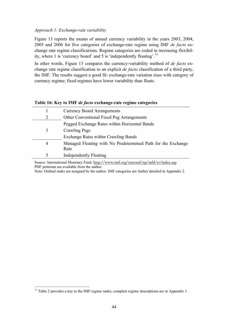
44
Approach 1: Exchange-rate variability
Figure 13 reports the means of annual currency variability in the years 2003, 2004, 2005 and 2006 for five categories of exchange-rate regime using IMF de facto ex-change rate regime classifications. Regime categories are coded in increasing flexibil-ity, where 1 is ‘currency board’ and 5 is ‘independently floating’.75
In other words, Figure 13 compares the currency-variability method of de facto ex-change rate regime classification to an explicit de facto classification of a third party, the IMF. The results suggest a good fit: exchange-rate variation rises with category of currency regime; fixed regimes have lower variability than floats.
Table 16: Key to IMF de facto exchange-rate regime categories
1 Currency Board Arrangements2 Other Conventional Fixed Peg Arrangements
Pegged Exchange Rates within Horizontal Bands3 Crawling Pegs
Exchange Rates within Crawling Bands4 Managed Floating with No Predetermined Path for the Exchange
Rate5 Independently Floating
Source: International Monetary Fund. http://www.imf.org/external/np/mfd/er/index.asp. PDF printouts are available from the author.Note: Ordinal ranks are assigned by the author. IMF categories are further detailed in Appendix 2.
75 Table 2 provides a key to the IMF regime ranks; complete regime descriptions are in Appendix 1.
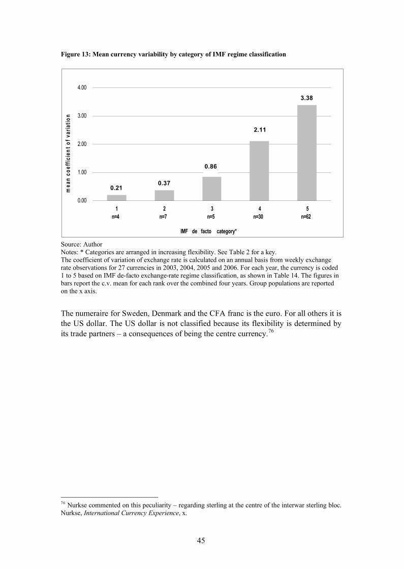
45
Figure 13: Mean currency variability by category of IMF regime classification
Source: AuthorNotes: * Categories are arranged in increasing flexibility. See Table 2 for a key.The coefficient of variation of exchange rate is calculated on an annual basis from weekly exchange rate observations for 27 currencies in 2003, 2004, 2005 and 2006. For each year, the currency is coded 1 to 5 based on IMF de-facto exchange-rate regime classification, as shown in Table 14. The figures in bars report the c.v. mean for each rank over the combined four years. Group populations are reported on the x axis.
The numeraire for Sweden, Denmark and the CFA franc is the euro. For all others it is the US dollar. The US dollar is not classified because its flexibility is determined by its trade partners – a consequences of being the centre currency.76
76 Nurkse commented on this peculiarity – regarding sterling at the centre of the interwar sterling bloc. Nurkse, International Currency Experience, x.
0.210.37
3.38
2.11
0.86
0.00
1.00
2.00
3.00
4.00
1n=4
2n=7
3n=5
4n=30
5n=62
IMF de facto category*
mea
nco
effic
ient
ofva
riatio
n
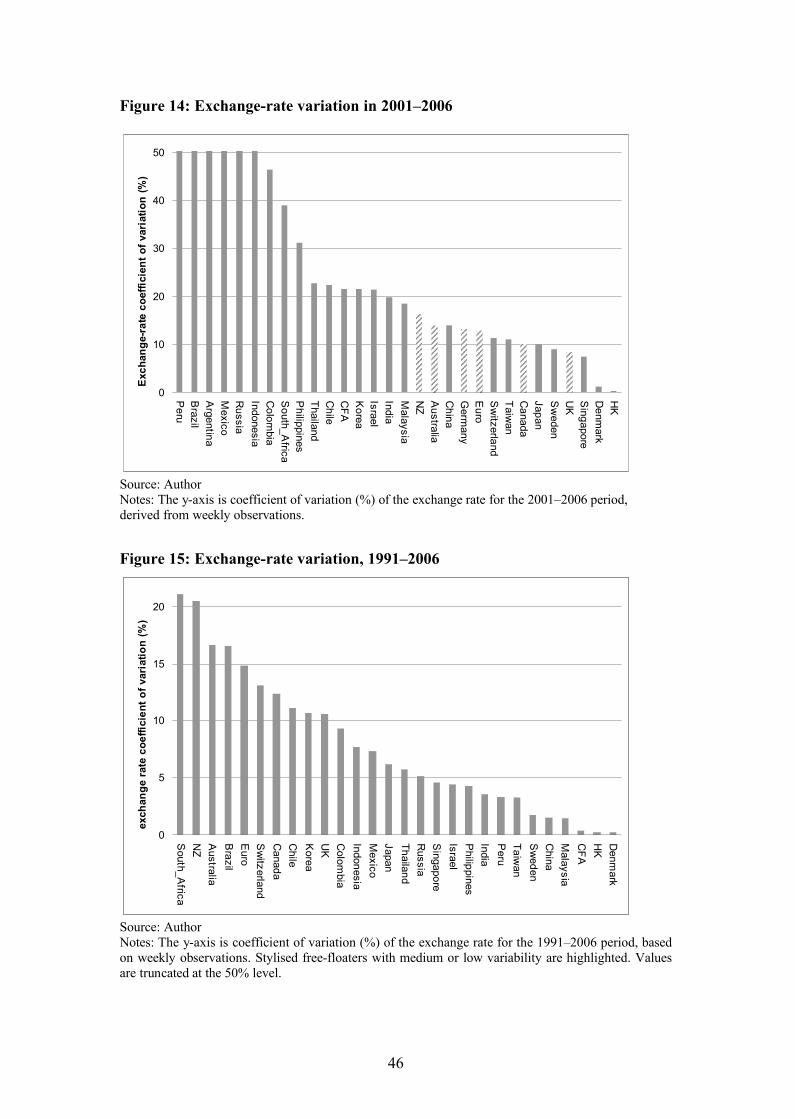
46
Figure 14: Exchange-rate variation in 2001–2006
Source: AuthorNotes: The y-axis is coefficient of variation (%) of the exchange rate for the 2001–2006 period,derived from weekly observations.
Figure 15: Exchange-rate variation, 1991–2006
Source: AuthorNotes: The y-axis is coefficient of variation (%) of the exchange rate for the 1991–2006 period, based on weekly observations. Stylised free-floaters with medium or low variability are highlighted. Values are truncated at the 50% level.
0
5
10
15
20S
outh_Africa
NZ
Australia
Brazil
Euro
Sw
itzerlandC
anadaC
hileK
oreaU
KC
olombia
IndonesiaM
exicoJapanThailandR
ussiaS
ingaporeIsraelP
hilippinesIndiaP
eruTaiw
anS
weden
China
Malaysia
CFA
HK
Denm
ark
exch
ange
rate
coef
ficie
ntof
vari
atio
n(%
)
0
10
20
30
40
50
Peru
Brazil
Argentina
Mexico
Russia
IndonesiaC
olombia
South_A
fricaP
hilippinesThailandC
hileC
FAK
oreaIsraelIndiaM
alaysiaN
ZA
ustraliaC
hinaG
ermany
Euro
Sw
itzerlandTaiw
anC
anadaJapanS
weden
UK
Singapore
Denm
arkH
K
Exc
hang
e-ra
teco
effic
ient
ofva
riat
ion
(%)
47
How does the methodology compare to stylised impressions of currency regime? Figure 14 ranks 28 currencies in the 2001–2006 period by coefficient of variation in exchange rates (in percentage terms).77 This compares the currency-variability meas-ure to stylised consensus views. Here too the outcome is satisfactory: stylised free floaters have the highest exchange-rate variability.
One problem with Figures 13 and 14 could be the sample: 2001–2006 was a calm period in international finance, with falling sovereign spreads and improving external balances outside of the United States. To incorporate more tumultuous periods, Figure 15 reports coefficient of variation for the 1991–2006 period. The results suggest that currency variability is misleading over longer periods, e.g. of 10 years or more. The most stable currencies are those whose regimes are commonly accepted to be free floating. Currency variability here misidentifies floats as pegs or intermediates.
Such a result is not surprising. In an actively traded foreign exchange market free of central bank interference, agents have an incentive to take positions which stabilise the exchange rate. Those with confidence in the fundamentals of a currency might use a period of inordinate weakness to purchase the currency and inordinate strength to sell. The net effect is to stabilise the exchange rate.
Figure 15 shows that exchange-rate outcome is also susceptible to misidentifying pegs and intermediates as floats. Pegs periodically succumb to devaluation pressures except where the currency appears undervalued (China) or where domestic wages and prices are downwardly flexible (Hong Kong). The result is a high variance statistic despite an underlying pegged regime. The key examples in Figure 15 are Malaysia and the Franc CFA (Communaut� financi�re d’Afrique). Both exhibit higher variance statistics than do the stylised floaters (highlighted in a lighter tone) yet are pegged re-gimes. Until July 1997 Malaysia had a de facto � 2% peg to the dollar, after which it transitioned to a tight dollar peg in October 1998. The Franc CFA was pegged throughout the 1991–2006 period; a one-time devaluation produces the high variance statistic.78
The key result is that an exchange-rate regime classification methodology relying exclusively on variation of the exchange rate will sometimes produce a ‘false posi-tive’ for a pegged regime which is in fact floating, and will sometimes produce a ‘false positive’ for a floating regime which is in fact pegged or otherwise rigid. It overlooks the possibility that a free float breeds stability.
77 Coefficient of variation is the standard deviation divided by the mean.78 Currency chronologies are catalogued in Reinhart and Rogoff, ‘The modern history of exchange-rate arrangements’, 54–104.
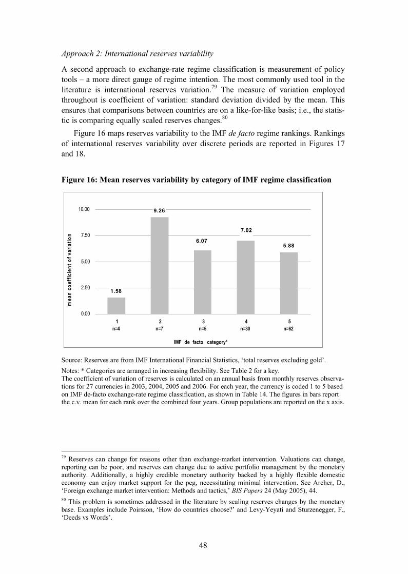
48
Approach 2: International reserves variability
A second approach to exchange-rate regime classification is measurement of policy tools – a more direct gauge of regime intention. The most commonly used tool in the literature is international reserves variation.79 The measure of variation employed throughout is coefficient of variation: standard deviation divided by the mean. This ensures that comparisons between countries are on a like-for-like basis; i.e., the statis-tic is comparing equally scaled reserves changes.80
Figure 16 maps reserves variability to the IMF de facto regime rankings. Rankings of international reserves variability over discrete periods are reported in Figures 17 and 18.
Figure 16: Mean reserves variability by category of IMF regime classification
Source: Reserves are from IMF International Financial Statistics, ‘total reserves excluding gold’.Notes: * Categories are arranged in increasing flexibility. See Table 2 for a key. The coefficient of variation of reserves is calculated on an annual basis from monthly reserves observa-tions for 27 currencies in 2003, 2004, 2005 and 2006. For each year, the currency is coded 1 to 5 based on IMF de-facto exchange-rate regime classification, as shown in Table 14. The figures in bars report the c.v. mean for each rank over the combined four years. Group populations are reported on the x axis.
79 Reserves can change for reasons other than exchange-market intervention. Valuations can change, reporting can be poor, and reserves can change due to active portfolio management by the monetary authority. Additionally, a highly credible monetary authority backed by a highly flexible domestic economy can enjoy market support for the peg, necessitating minimal intervention. See Archer, D., ‘Foreign exchange market intervention: Methods and tactics,’ BIS Papers 24 (May 2005), 44. 80 This problem is sometimes addressed in the literature by scaling reserves changes by the monetary base. Examples include Poirsson, ‘How do countries choose?’ and Levy-Yeyati and Sturzenegger, F., ‘Deeds vs Words’.
1.58
9.26
5.88
7.02
6.07
0.00
2.50
5.00
7.50
10.00
1n=4
2n=7
3n=5
4n=30
5n=62
IMF de facto category*
mea
nco
effic
ient
ofva
riatio
n
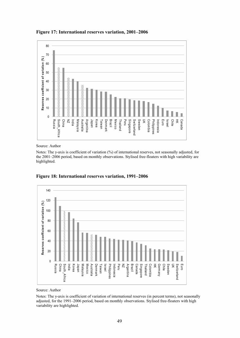
49
Figure 17: International reserves variation, 2001–2006
Source: AuthorNotes: The y-axis is coefficient of variation (%) of international reserves, not seasonally adjusted, for the 2001–2006 period, based on monthly observations. Stylised free-floaters with high variability are highlighted.
Figure 18: International reserves variation, 1991–2006
Source: AuthorNotes: The y-axis is coefficient of variation of international reserves (in percent terms), not seasonally adjusted, for the 1991–2006 period, based on monthly observations. Stylised free-floaters with high variability are highlighted.
0
10
20
30
40
50
60
70
80
Russia
South_A
fricaC
hinaN
ZIndiaM
alaysiaA
ustraliaA
rgentinaJapanK
oreaTaiw
anD
enmark
Brazil
Mexico
ThailandP
eruS
ingaporeS
witzerland
Sw
edenU
KC
olombia
Philippines
IndonesiaE
uroIsraelC
hileH
KC
anada
Rese
rves
coef
ficie
ntof
varia
tion
(%)
0
20
40
60
80
100
120
140
Russia
China
South_A
fricaIndiaK
oreaJapanM
alaysiaM
exicoA
ustraliaD
enmark
Taiwan
IsraelP
hilippinesIndonesiaP
eruN
ZA
rgentinaB
razilC
anadaS
ingaporeThailandC
olombia
HK
Germ
anyC
hileS
weden
UK
Sw
itzerlandE
uro
Rese
rves
coef
ficie
ntof
varia
tion
(%)
50
Figure 16 suggests that reserve variation does not map well to IMF de facto re-gime coding. Figure 17 improves the validity of this measure vis-�-vis stylised con-sensus views on currency regimes. For example, Canada displays the lowest reserves variation in the group, and the UK and euro-area are among the lowest. Nevertheless, anomalous results include high variability for South Africa and Australia, which are both commonly understood to maintain floating exchange-rate regimes.
Reserves variation produces fewer ‘false positives’ for regime type than does cur-rency variation. Yet a significant anomaly in the reported reserves results is Hong Kong. Its currency board regime, an extreme form of currency peg, would be incor-rectly identified as a highly flexible regime due to the low variability in reserves.81
Flexibility indices
These methodologies are sometimes combined into a composite index measuring de-gree of currency regime flexibility.82 For the index to be increasing in regime flexibil-ity, outcome-based measures (e.g. exchange-rate variability) are in the numerator and policy-based measures (e.g. reserves variability) are in the denominator. Activist use of policy instruments suggests greater intervention in the foreign exchange market and hence a lower degree of floating.83
The performance of such indices can be judged from application to modern data. Fig-ure 19 reports results from a generic index, to be called here ‘Lamda-standard’. Its numerator is coefficient of variation of the exchange rate and denominator is coeffi-cient of variation of reserves. Figures 20 and 21 report individual currency results for the periods 2001–2006 and 1991–2006 respectively.
81 As highlighted in footnote 42.82 Calvo and Reinhart, ‘Fear of floating’, 400 and Poirson, ‘How do countries choose?’. 83 The short-term policy interest rate is another measurable instrument. See footnote 26.
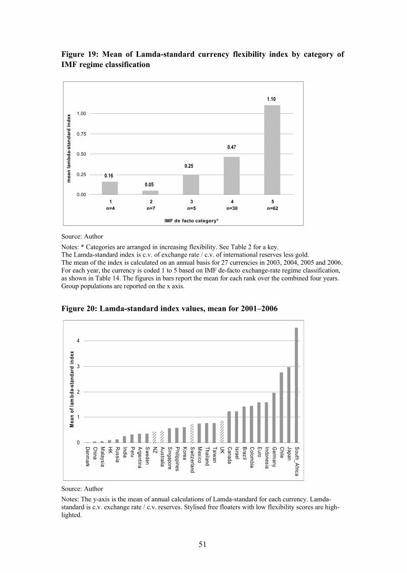
51
Figure 19: Mean of Lamda-standard currency flexibility index by category of IMF regime classification
Source: AuthorNotes: * Categories are arranged in increasing flexibility. See Table 2 for a key.The Lamda-standard index is c.v. of exchange rate / c.v. of international reserves less gold. The mean of the index is calculated on an annual basis for 27 currencies in 2003, 2004, 2005 and 2006. For each year, the currency is coded 1 to 5 based on IMF de-facto exchange-rate regime classification, as shown in Table 14. The figures in bars report the mean for each rank over the combined four years. Group populations are reported on the x axis.
Figure 20: Lamda-standard index values, mean for 2001–2006
Source: AuthorNotes: The y-axis is the mean of annual calculations of Lamda-standard for each currency. Lamda-standard is c.v. exchange rate / c.v. reserves. Stylised free floaters with low flexibility scores are high-lighted.
0.160.05
1.10
0.25
0.47
0.00
0.25
0.50
0.75
1.00
1n=4
2n=7
3n=5
4n=30
5n=62
IMF de facto category*
mea
nla
mbd
a-st
anda
rdin
dex
0
1
2
3
4
Denm
arkC
hinaM
alaysiaH
KR
ussiaIndiaP
eruA
rgentinaS
wedenN
ZA
ustraliaS
ingaporeP
hilippinesK
oreaS
witzerlandM
exicoThailandTaiw
anU
KC
anadaIsraelB
razilC
olombia
Euro
IndonesiaG
ermany
Chile
JapanS
outh_Africa
Mea
nof
lam
bda-
stan
dard
inde
x
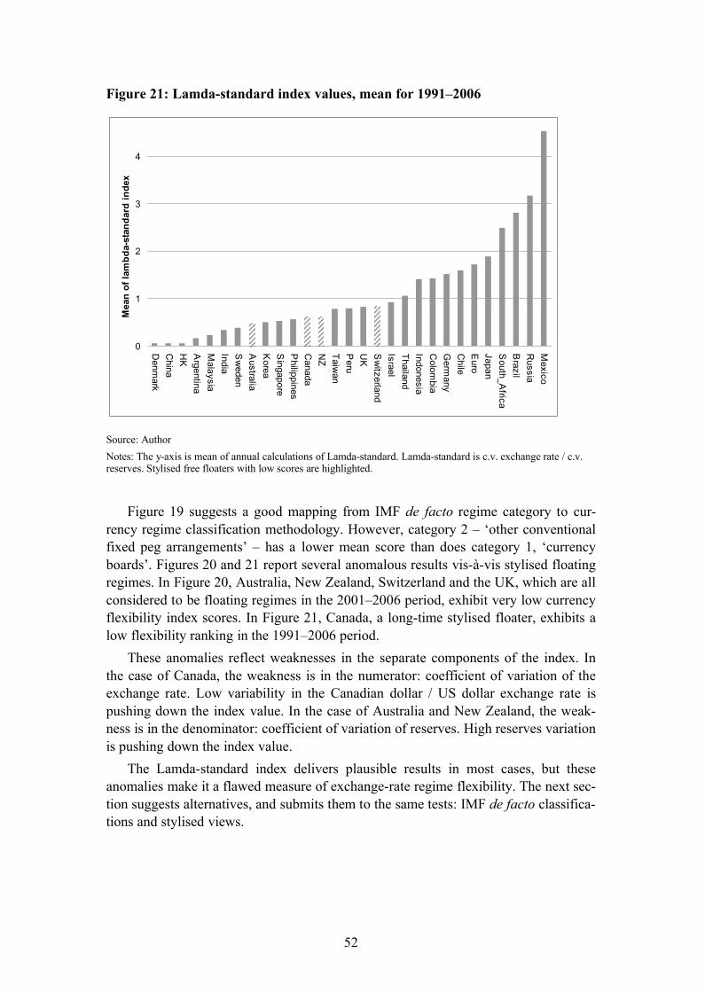
52
Figure 21: Lamda-standard index values, mean for 1991–2006
Source: AuthorNotes: The y-axis is mean of annual calculations of Lamda-standard. Lamda-standard is c.v. exchange rate / c.v. reserves. Stylised free floaters with low scores are highlighted.
Figure 19 suggests a good mapping from IMF de facto regime category to cur-rency regime classification methodology. However, category 2 – ‘other conventional fixed peg arrangements’ – has a lower mean score than does category 1, ‘currency boards’. Figures 20 and 21 report several anomalous results vis-�-vis stylised floating regimes. In Figure 20, Australia, New Zealand, Switzerland and the UK, which are all considered to be floating regimes in the 2001–2006 period, exhibit very low currency flexibility index scores. In Figure 21, Canada, a long-time stylised floater, exhibits a low flexibility ranking in the 1991–2006 period.
These anomalies reflect weaknesses in the separate components of the index. In the case of Canada, the weakness is in the numerator: coefficient of variation of the exchange rate. Low variability in the Canadian dollar / US dollar exchange rate is pushing down the index value. In the case of Australia and New Zealand, the weak-ness is in the denominator: coefficient of variation of reserves. High reserves variation is pushing down the index value.
The Lamda-standard index delivers plausible results in most cases, but these anomalies make it a flawed measure of exchange-rate regime flexibility. The next sec-tion suggests alternatives, and submits them to the same tests: IMF de facto classifica-tions and stylised views.
0
1
2
3
4
Denm
arkC
hinaH
KA
rgentinaM
alaysiaIndiaS
weden
Australia
Korea
Singapore
Philippines
Canada
NZ
Taiwan
Peru
UK
Sw
itzerlandIsraelThailandIndonesiaC
olombia
Germ
anyC
hileE
uroJapanS
outh_Africa
Brazil
Russia
Mexico
Mea
nof
lam
bda-
stan
dard
inde
x
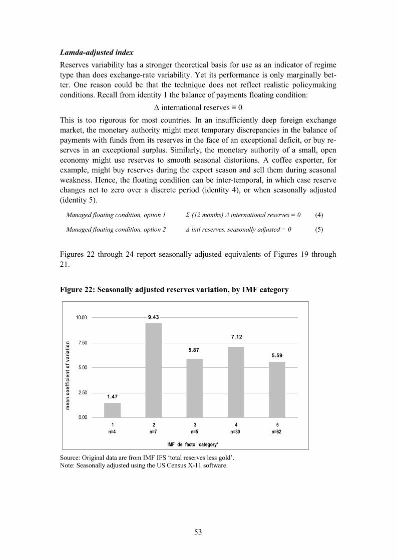
53
Lamda-adjusted indexReserves variability has a stronger theoretical basis for use as an indicator of regime type than does exchange-rate variability. Yet its performance is only marginally bet-ter. One reason could be that the technique does not reflect realistic policymaking conditions. Recall from identity 1 the balance of payments floating condition:
Δ international reserves ≡ 0This is too rigorous for most countries. In an insufficiently deep foreign exchange market, the monetary authority might meet temporary discrepancies in the balance of payments with funds from its reserves in the face of an exceptional deficit, or buy re-serves in an exceptional surplus. Similarly, the monetary authority of a small, open economy might use reserves to smooth seasonal distortions. A coffee exporter, for example, might buy reserves during the export season and sell them during seasonal weakness. Hence, the floating condition can be inter-temporal, in which case reserve changes net to zero over a discrete period (identity 4), or when seasonally adjusted (identity 5).
Managed floating condition, option 1 Σ (12 months) Δ international reserves = 0 (4)
Managed floating condition, option 2 Δ intl reserves, seasonally adjusted = 0 (5)
Figures 22 through 24 report seasonally adjusted equivalents of Figures 19 through 21.
Figure 22: Seasonally adjusted reserves variation, by IMF category
Source: Original data are from IMF IFS ‘total reserves less gold’. Note: Seasonally adjusted using the US Census X-11 software.
1.47
9.43
5.595.87
7.12
0.00
2.50
5.00
7.50
10.00
1n=4
2n=7
3n=5
4n=30
5n=62
IMF de facto category*
mea
nco
effic
ient
ofva
riatio
n
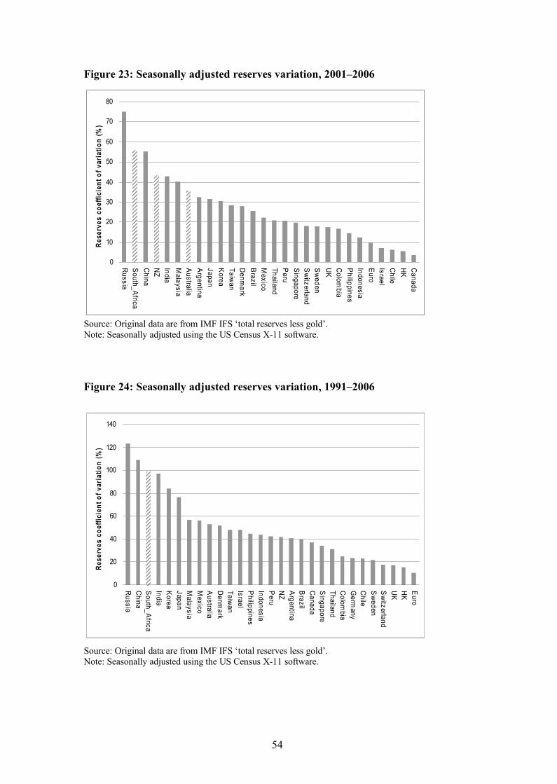
54
Figure 23: Seasonally adjusted reserves variation, 2001–2006
Source: Original data are from IMF IFS ‘total reserves less gold’. Note: Seasonally adjusted using the US Census X-11 software.
Figure 24: Seasonally adjusted reserves variation, 1991–2006
Source: Original data are from IMF IFS ‘total reserves less gold’. Note: Seasonally adjusted using the US Census X-11 software.
0
10
20
30
40
50
60
70
80
Russia
South_A
fricaC
hinaN
ZIndiaM
alaysiaA
ustraliaA
rgentinaJapanK
oreaTaiw
anD
enmark
Brazil
Mexico
ThailandP
eruS
ingaporeS
witzerland
Sw
edenU
KC
olombia
Philippines
IndonesiaE
uroIsraelC
hileH
KC
anada
Rese
rves
coef
ficie
ntof
vari
atio
n(%
)
0
20
40
60
80
100
120
140R
ussiaC
hinaS
outh_Africa
IndiaK
oreaJapanM
alaysiaM
exicoA
ustraliaD
enmark
Taiwan
IsraelP
hilippinesIndonesiaP
eruN
ZA
rgentinaB
razilC
anadaS
ingaporeThailandC
olombia
Germ
anyC
hileS
weden
Sw
itzerlandU
KH
KE
uro
Rese
rves
coef
ficie
ntof
vari
atio
n(%
)
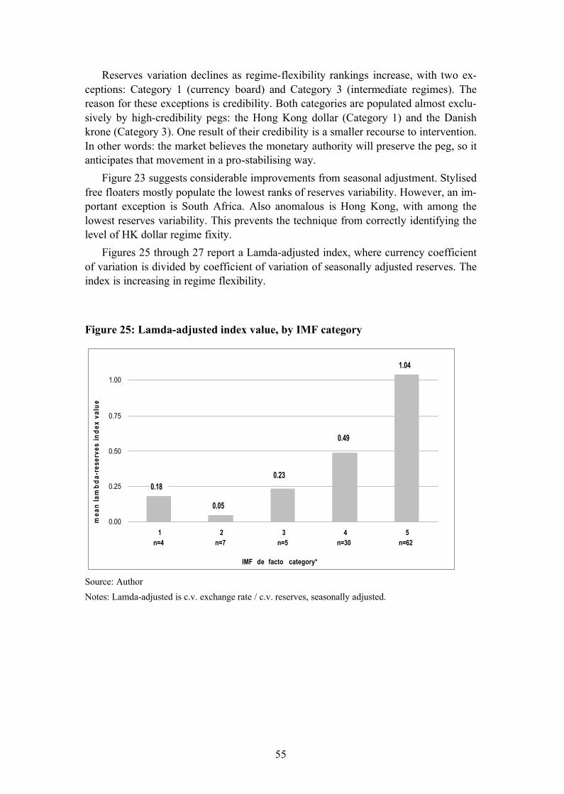
55
Reserves variation declines as regime-flexibility rankings increase, with two ex-ceptions: Category 1 (currency board) and Category 3 (intermediate regimes). The reason for these exceptions is credibility. Both categories are populated almost exclu-sively by high-credibility pegs: the Hong Kong dollar (Category 1) and the Danish krone (Category 3). One result of their credibility is a smaller recourse to intervention. In other words: the market believes the monetary authority will preserve the peg, so it anticipates that movement in a pro-stabilising way.
Figure 23 suggests considerable improvements from seasonal adjustment. Stylised free floaters mostly populate the lowest ranks of reserves variability. However, an im-portant exception is South Africa. Also anomalous is Hong Kong, with among the lowest reserves variability. This prevents the technique from correctly identifying the level of HK dollar regime fixity.
Figures 25 through 27 report a Lamda-adjusted index, where currency coefficient of variation is divided by coefficient of variation of seasonally adjusted reserves. The index is increasing in regime flexibility.
Figure 25: Lamda-adjusted index value, by IMF category
Source: AuthorNotes: Lamda-adjusted is c.v. exchange rate / c.v. reserves, seasonally adjusted.
0.18
0.05
1.04
0.49
0.23
0.00
0.25
0.50
0.75
1.00
1n=4
2n=7
3n=5
4n=30
5n=62
IMF de facto category*
mea
nla
mbd
a-re
serv
esin
dex
valu
e
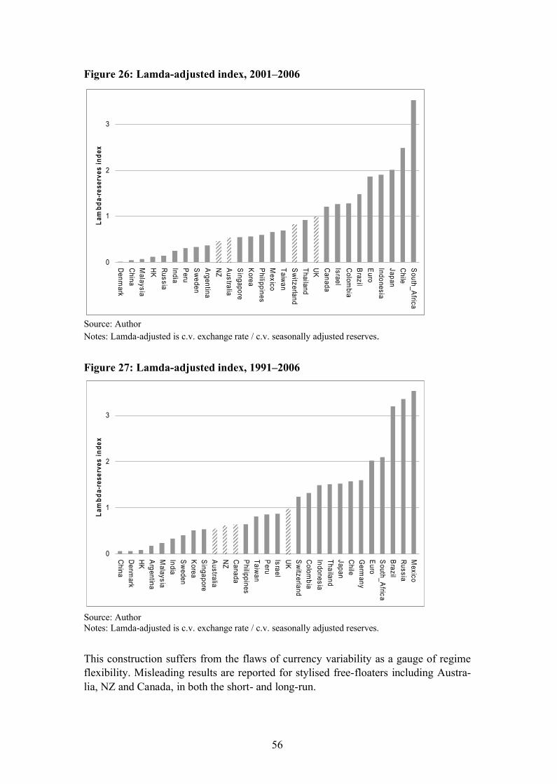
56
Figure 26: Lamda-adjusted index, 2001–2006
Source: AuthorNotes: Lamda-adjusted is c.v. exchange rate / c.v. seasonally adjusted reserves.
Figure 27: Lamda-adjusted index, 1991–2006
Source: AuthorNotes: Lamda-adjusted is c.v. exchange rate / c.v. seasonally adjusted reserves.
This construction suffers from the flaws of currency variability as a gauge of regime flexibility. Misleading results are reported for stylised free-floaters including Austra-lia, NZ and Canada, in both the short- and long-run.
0
1
2
3
Denm
arkC
hinaM
alaysiaH
KR
ussiaIndiaP
eruS
weden
Argentina
NZ
Australia
Singapore
Korea
Philippines
Mexico
Taiwan
Sw
itzerlandThailandU
KC
anadaIsraelC
olombia
Brazil
Euro
IndonesiaJapanC
hileS
outh_Africa
Lam
bda-
rese
rves
inde
x
0
1
2
3
China
Denm
arkH
KA
rgentinaM
alaysiaIndiaS
weden
Korea
Singapore
Australia
NZ
Canada
Philippines
Taiwan
Peru
IsraelU
KS
witzerland
Colom
biaIndonesiaThailandJapanC
hileG
ermany
Euro
South_A
fricaB
razilR
ussiaM
exico
Lam
bda-
rese
rves
inde
x
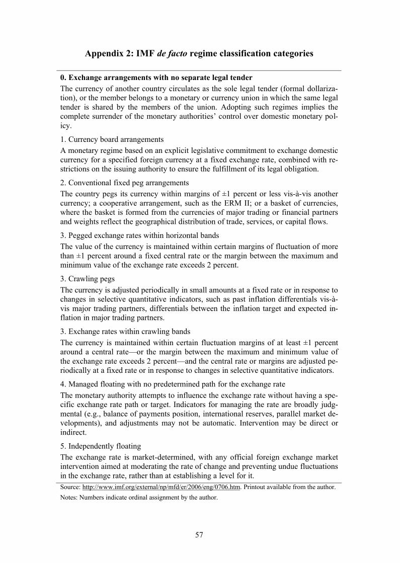
57
Appendix 2: IMF de facto regime classification categories
0. Exchange arrangements with no separate legal tenderThe currency of another country circulates as the sole legal tender (formal dollariza-tion), or the member belongs to a monetary or currency union in which the same legal tender is shared by the members of the union. Adopting such regimes implies the complete surrender of the monetary authorities’ control over domestic monetary pol-icy.
1. Currency board arrangementsA monetary regime based on an explicit legislative commitment to exchange domestic currency for a specified foreign currency at a fixed exchange rate, combined with re-strictions on the issuing authority to ensure the fulfillment of its legal obligation.
2. Conventional fixed peg arrangementsThe country pegs its currency within margins of �1 percent or less vis-�-vis another currency; a cooperative arrangement, such as the ERM II; or a basket of currencies, where the basket is formed from the currencies of major trading or financial partners and weights reflect the geographical distribution of trade, services, or capital flows.
3. Pegged exchange rates within horizontal bandsThe value of the currency is maintained within certain margins of fluctuation of more than �1 percent around a fixed central rate or the margin between the maximum and minimum value of the exchange rate exceeds 2 percent.
3. Crawling pegsThe currency is adjusted periodically in small amounts at a fixed rate or in response to changes in selective quantitative indicators, such as past inflation differentials vis-�-vis major trading partners, differentials between the inflation target and expected in-flation in major trading partners.
3. Exchange rates within crawling bandsThe currency is maintained within certain fluctuation margins of at least �1 percent around a central rate—or the margin between the maximum and minimum value of the exchange rate exceeds 2 percent—and the central rate or margins are adjusted pe-riodically at a fixed rate or in response to changes in selective quantitative indicators.
4. Managed floating with no predetermined path for the exchange rateThe monetary authority attempts to influence the exchange rate without having a spe-cific exchange rate path or target. Indicators for managing the rate are broadly judg-mental (e.g., balance of payments position, international reserves, parallel market de-velopments), and adjustments may not be automatic. Intervention may be direct or indirect.
5. Independently floatingThe exchange rate is market-determined, with any official foreign exchange market intervention aimed at moderating the rate of change and preventing undue fluctuations in the exchange rate, rather than at establishing a level for it.Source: http://www.imf.org/external/np/mfd/er/2006/eng/0706.htm. Printout available from the author.Notes: Numbers indicate ordinal assignment by the author.
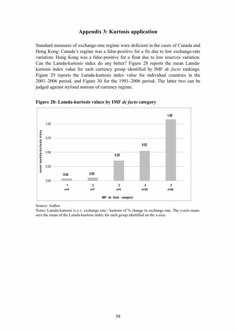
58
Appendix 3: Kurtosis application
Standard measures of exchange-rate regime were deficient in the cases of Canada and Hong Kong: Canada’s regime was a false-positive for a fix due to low exchange-rate variation; Hong Kong was a false-positive for a float due to low reserves variation. Can the Lamda-kurtosis index do any better? Figure 28 reports the mean Lamda-kurtosis index value for each currency group identified by IMF de facto rankings. Figure 29 reports the Lamda-kurtosis index value for individual countries in the 2001–2006 period, and Figure 30 for the 1991–2006 period. The latter two can be judged against stylised notions of currency regime.
Figure 28: Lamda-kurtosis values by IMF de facto category
Source: AuthorNotes: Lamda-kurtosis is c.v. exchange rate / kurtosis of % change in exchange rate. The y-axis meas-ures the mean of the Lamda-kurtosis index for each group identified on the x-axis.
0.04 0.05
1.08
0.35
0.52
0.00
0.25
0.50
0.75
1.00
1n=4
2n=7
3n=5
4n=30
5n=62
IMF de facto category*
mea
nla
mbd
a-ku
rtos
isin
dex
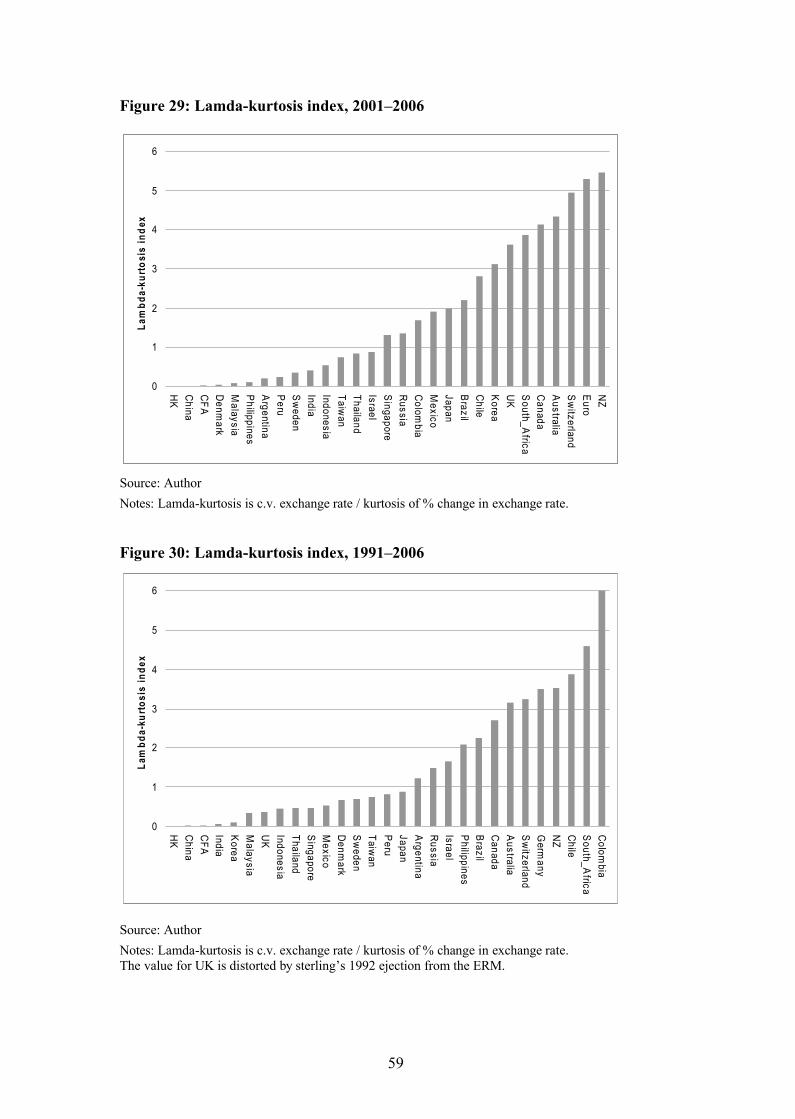
59
Figure 29: Lamda-kurtosis index, 2001–2006
Source: AuthorNotes: Lamda-kurtosis is c.v. exchange rate / kurtosis of % change in exchange rate.
Figure 30: Lamda-kurtosis index, 1991–2006
Source: AuthorNotes: Lamda-kurtosis is c.v. exchange rate / kurtosis of % change in exchange rate. The value for UK is distorted by sterling’s 1992 ejection from the ERM.
0
1
2
3
4
5
6
HK
China
CFA
Denm
arkM
alaysiaP
hilippinesA
rgentinaP
eruS
weden
IndiaIndonesiaTaiw
anThailandIsraelS
ingaporeR
ussiaC
olombia
Mexico
JapanB
razilC
hileK
oreaU
KS
outh_Africa
Canada
Australia
Sw
itzerlandE
uroN
Z
Lam
bda-
kurto
sis
inde
x
0
1
2
3
4
5
6
HK
China
CFA
IndiaK
oreaM
alaysiaU
KIndonesiaThailandS
ingaporeM
exicoD
enmark
Sw
edenTaiw
anP
eruJapanA
rgentinaR
ussiaIsraelP
hilippinesB
razilC
anadaA
ustraliaS
witzerland
Germ
anyN
ZC
hileS
outh_Africa
Colom
bia
Lam
bda-
kurto
sis
inde
x
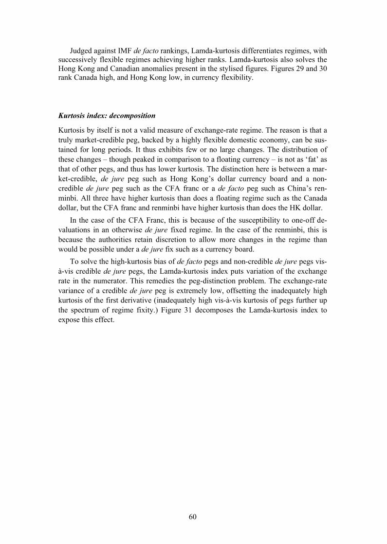
60
Judged against IMF de facto rankings, Lamda-kurtosis differentiates regimes, with successively flexible regimes achieving higher ranks. Lamda-kurtosis also solves the Hong Kong and Canadian anomalies present in the stylised figures. Figures 29 and 30 rank Canada high, and Hong Kong low, in currency flexibility.
Kurtosis index: decomposition
Kurtosis by itself is not a valid measure of exchange-rate regime. The reason is that a truly market-credible peg, backed by a highly flexible domestic economy, can be sus-tained for long periods. It thus exhibits few or no large changes. The distribution of these changes – though peaked in comparison to a floating currency – is not as ‘fat’ as that of other pegs, and thus has lower kurtosis. The distinction here is between a mar-ket-credible, de jure peg such as Hong Kong’s dollar currency board and a non-credible de jure peg such as the CFA franc or a de facto peg such as China’s ren-minbi. All three have higher kurtosis than does a floating regime such as the Canada dollar, but the CFA franc and renminbi have higher kurtosis than does the HK dollar.
In the case of the CFA Franc, this is because of the susceptibility to one-off de-valuations in an otherwise de jure fixed regime. In the case of the renminbi, this is because the authorities retain discretion to allow more changes in the regime than would be possible under a de jure fix such as a currency board.
To solve the high-kurtosis bias of de facto pegs and non-credible de jure pegs vis-�-vis credible de jure pegs, the Lamda-kurtosis index puts variation of the exchange rate in the numerator. This remedies the peg-distinction problem. The exchange-rate variance of a credible de jure peg is extremely low, offsetting the inadequately high kurtosis of the first derivative (inadequately high vis-�-vis kurtosis of pegs further up the spectrum of regime fixity.) Figure 31 decomposes the Lamda-kurtosis index to expose this effect.
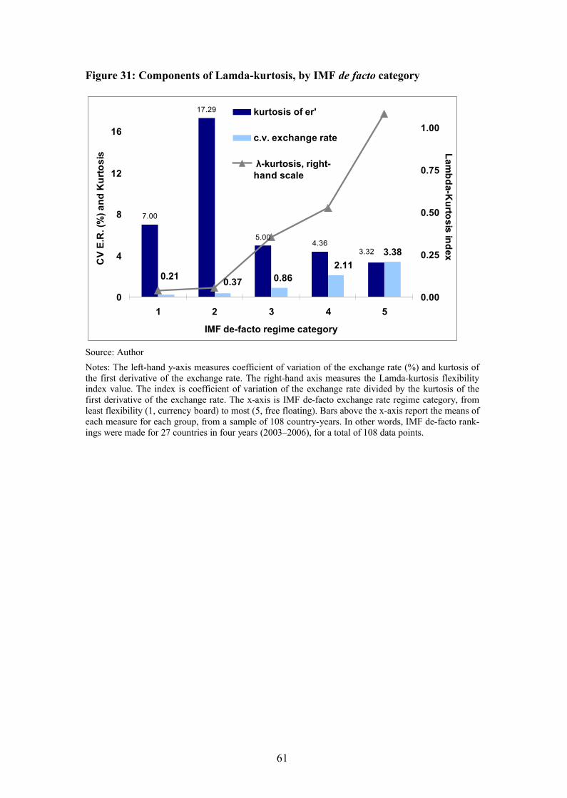
61
Figure 31: Components of Lamda-kurtosis, by IMF de facto category
Source: AuthorNotes: The left-hand y-axis measures coefficient of variation of the exchange rate (%) and kurtosis of the first derivative of the exchange rate. The right-hand axis measures the Lamda-kurtosis flexibility index value. The index is coefficient of variation of the exchange rate divided by the kurtosis of the first derivative of the exchange rate. The x-axis is IMF de-facto exchange rate regime category, from least flexibility (1, currency board) to most (5, free floating). Bars above the x-axis report the means of each measure for each group, from a sample of 108 country-years. In other words, IMF de-facto rank-ings were made for 27 countries in four years (2003–2006), for a total of 108 data points.
7.00
17.29
5.004.36
3.383.32
2.110.860.370.21
0
4
8
12
16
1 2 3 4 5
IMF de-facto regime category
CV
E.R
.(%
)and
Kur
tosi
s
0.00
0.25
0.50
0.75
1.00Lam
bda-Kurtosis
indexkurtosis of er'
c.v. exchange rate
λ-kurtosis, right-hand scale
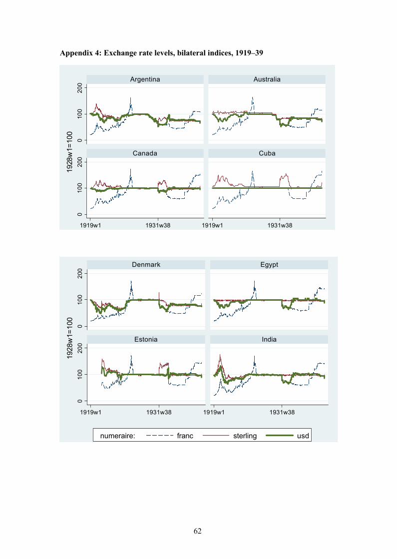
62
Appendix 4: Exchange rate levels, bilateral indices, 1919–39
010
020
00
100
200
1919w1 1931w38 1919w1 1931w38
Denmark Egypt
Estonia India
numeraire: franc sterling usd
1928
w1=
100
010
020
00
100
200
1919w1 1931w38 1919w1 1931w38
Argentina Australia
Canada Cuba
1928
w1=
100
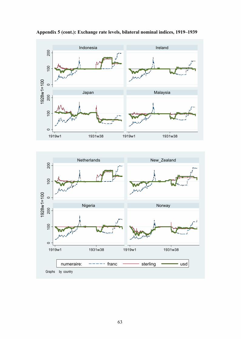
63
Appendix 5 (cont.): Exchange rate levels, bilateral nominal indices, 1919–1939
010
020
00
100
200
1919w1 1931w38 1919w1 1931w38
Netherlands New_Zealand
Nigeria Norway
numeraire: franc sterling usd
1928
w1=
100
Graphs by country
010
020
00
100
200
1919w1 1931w38 1919w1 1931w38
Indonesia Ireland
Japan Malaysia
1928
w1=
100
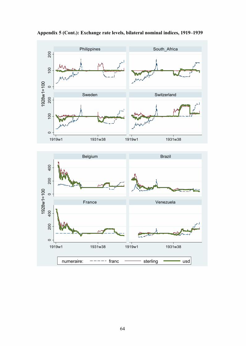
64
Appendix 5 (Cont.): Exchange rate levels, bilateral nominal indices, 1919–1939
010
020
00
100
200
1919w1 1931w38 1919w1 1931w38
Philippines South_Africa
Sweden Switzerland
1928
w1=
100
020
040
00
200
400
1919w1 1931w38 1919w1 1931w38
Belgium Brazil
France Venezuela
numeraire: franc sterling usd
1928
w1=
100
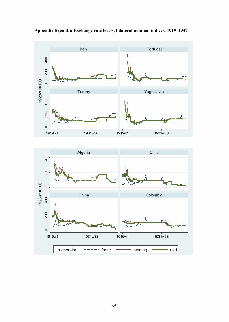
65
Appendix 5 (cont.): Exchange rate levels, bilateral nominal indices, 1919–1939
020
040
00
200
400
1919w1 1931w38 1919w1 1931w38
Algeria Chile
China Colombia
numeraire: franc sterling usd
1928
w1=
100
020
040
00
200
400
1919w1 1931w38 1919w1 1931w38
Italy Portugal
Turkey Yugoslavia
1928
w1=
100
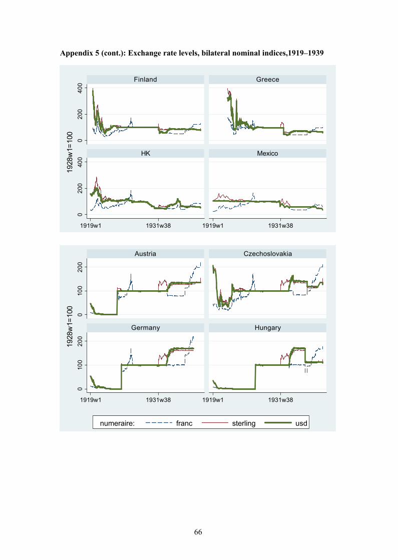
66
Appendix 5 (cont.): Exchange rate levels, bilateral nominal indices,1919–1939
020
040
00
200
400
1919w1 1931w38 1919w1 1931w38
Finland Greece
HK Mexico
1928
w1=
100
010
020
00
100
200
1919w1 1931w38 1919w1 1931w38
Austria Czechoslovakia
Germany Hungary
numeraire: franc sterling usd
1928
w1=
100
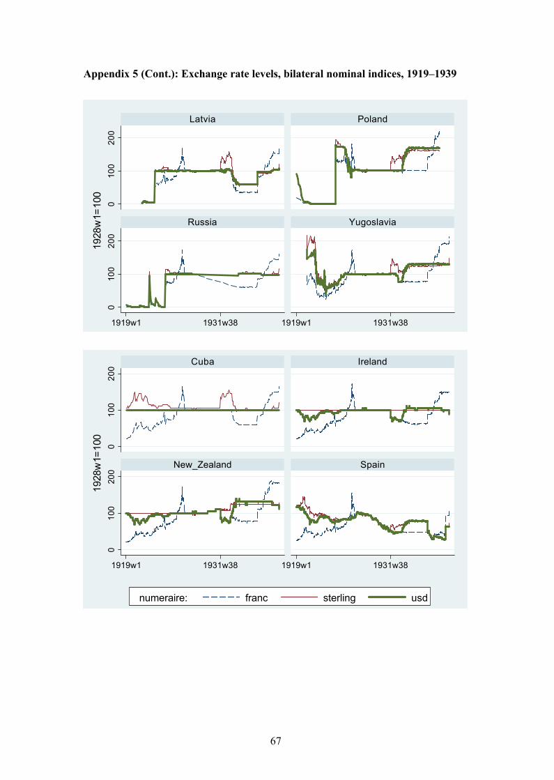
67
Appendix 5 (Cont.): Exchange rate levels, bilateral nominal indices, 1919–1939
010
020
00
100
200
1919w1 1931w38 1919w1 1931w38
Latvia Poland
Russia Yugoslavia
1928
w1=
100
010
020
00
100
200
1919w1 1931w38 1919w1 1931w38
Cuba Ireland
New_Zealand Spain
numeraire: franc sterling usd
1928
w1=
100
68
University of Oxford Discussion Papersin Economic and Social History: Recent publications
61 Natalia Mora-Sitja, Exploring Changes in Earnings Inequality during Industriali-zation: Barcelona, 1856–1905 (April 2006)
62 Camilla Brautaset and Regina Grafe, The Quiet Transport Revolution: Returns to Scale, Scope and Network Density in Norway’s Nineteenth-Century Sailing Fleet(June 2006)
63 Mohammad Niaz Asadullah, Educational Disparity in East and West Pakistan, 1947–71: Was East Pakistan Discriminated Against? (July 2006)
64 Jane Humphries, ‘Because they are too menny…’ Children, Mothers, and Fertil-ity Decline: The Evidence from Working-Class Autobiographies of the Eighteenth and Nineteenth Centuries (September 2006)
65 M. A. Irigoin and R. Grafe, Bargaining for Absolutism: A Spanish Path to Nation State and Empire Building (November 2006)
66 Jane Humphries and Tim Leunig, Cities, market integration and going to sea: stunting and the standard of living in early nineteenth-century England and Wales (March 2007)
67 Paul Sharp and Jacob Weisdorf, From Preventive to Permissive Checks: The Changing Nature of The Malthusian Relationship between Nuptiality and the Price of Provisions in the Nineteenth Century (November 2007)
68 Roman Studer, India and the Great Divergence: Assessing the Efficiency of Grain Markets in Eighteenth- and Nineteenth-Century India (November 2007)
69 Guillaume Daudin, Domestic Trade and Market Size in Late Eighteenth-Century France (April 2008)
70 Avner Offer, Charles Feinstein (1932–2005) and British Historical National Ac-counts (June 2008)
71 Sandra Gonz�lez-Bail�n and Tommy Murphy, When Smaller Families Look Con-tagious: A Spatial Look at the French Fertility Decline Using an Agent-based Simulation Model (September 2008)
72 Luke Samy, The Building Society Promise: Building Societies and Home Owner-ship, c1880–1913 (October 2008)
73. Leigh A. Gardner, To Take or to Make? Contracting for Legitimacy in the Emerging States of Twelfth-Century Britain (November 2008)
74. Avner Offer, British Manual Workers: From Producers to Consumers, c.1950–2000
75 Pablo Astorga, A Century of Economic Growth in Latin America (January 2009)
76 Scott Andrew Urban: The Name of the Rose: Classifying 1930s Exchange-Rate Regimes (April 2009)
UNIVERSITY OF OXFORD DISCUSSION PAPERSIN ECONOMIC AND SOCIAL HISTORY
are edited byRui Esteves (Brasenose College, Oxford, OX1 4AJ)Leigh Gardner (Jesus College, Oxford, OX1 3DW)
Papers may be downloaded fromhttp://www.nuff.ox.ac.uk/Economics/History