Embed Size (px)
Citation preview

SN 590E Vol. 1. Pg. 1, Ronald Green
SCIENTIFIC NOTEBOOK E590
Volume 1
by
Ronald Green
Southwest Research Institute Center for Nuclear Waste Regulatory Analyses
San Antonio, Texas
May 21, 2003

SN 590E Vol. 1. Pg. 2, Ronald Green
Table of Contents INITIAL ENTRIES: Continuation of the laboratory-scale heater test (lst) analyses ...................... June 16, 2003. Description of MULTIFLO systematic sensitivity analyses………..........3 Table 1. Summary of lst analyses: fracture, lst155 through lst172.………………………4 Table 2. Summary of lst analyses: matrix, lst155 through lst172........................................4 Sample input file: lst155.dat……………………………………………………………...6 Calculation of relative permeability for active fracture model…………………………..10 Matrix saturation: measured at the conclusion of test 2………...………………………11 Matrix saturation: simulated, runs lst155 through lst172……………………………….12 Matrix temperature: simulated, runs lst155 through lst172……………………………..17 Fracture saturation: simulated, runs lst155 through lst172……………………………...24 Sensitivity analysis of the effect of matrix/fracture permeability changes………………42 Table 3. Summary of lst analyses: fracture, lst173 through lst185, lst188………………42 Table 4. Summary of lst analyses: matrix, lst173 through lst185, lst188 ......................42 Matrix saturation: simulated, runs lst155 through lst172……………………………….44 Matrix temperature: simulated, runs lst155 through lst172……………………………..49 Fracture saturation: simulated, runs lst155 through lst172……………………………...55 Listing of relative permeability values…………………………………………………..69 Table 5. Fracture to fracture relative permeability………………………………………70 Table 6. Fracture to matrix relative permeability………………………………………..73 Appendix: mathematica notebook AFM_lst_186.nb for active fracture model relative permeability…………………………………………………………………………….1-7

SN 590E Vol. 1. Pg. 3, Ronald Green
INITIAL ENTRIES
Scientific notebook: #590E Vol. 1 Issued to: R.T. Green Issue Date: 21-May-2003
A series of MULTIFLO simulations are performed to examine data collected during the two lab-scale heater tests described in Scientific Notebook 209. All simulations were performed with MULTIFLO Version 1.5.2 August 2002. The objective of the analyses is to systematically vary different input parameters for numerical simulations of the lab-scale heater tests. The parameters in question include property values and conceptual model selections. Included are the AFM and the choice of gamma (either 0.2 or 0.4) when the AFM is invoked. If the AFM is not invoked, the effect of the areamodf is evaluated. Areamodf values assessed were 1.0, 0.1, and 0.001. Also assessed with the areadmodf was decoupling energy from mass. This decoupling is accomplished in the DCMPARAM input line. DCMPARA : i1 i2 j1 j2 k1 k2 volf areamodf xlm ylm zlm 1 24 1 14 1 30 0.050 1.0 .05 0.03 .05 -5 ! matrix Note that the 1.0 entry under areamodf, before the xlm category is where values for areamodf are entered for coupled systems. When coupled, both energy (heat) and mass interaction between the continua are limited. For decoupled systems (i.e., energy communication is not decreased when mass is decreased), the 1.0 is maintained below the areamodf, but the –5 is replaced with a numerical value (i.e., 0.1) for the areamodf value. The –5 designation is for the AFM (active fracture model). The relative permeability for unit 5 is described in the Pckr section of the input file. Also varied was the van Genuchten alpha value (equivalent to the inverse of t the air entry value). Values of 1e-3 and 1e-4 were considered. Runs lst155 through lst172 were performed as part of this analysis. lst155 was assumed to be the basecase with on AFM, an alpha of 1e-4, and no reduction in areamodf. The 18 runs are described in Table 1. Dec indicates whether heat transfer is decoupled from mass transfer.

SN 590E Vol. 1. Pg. 4, Ronald Green
Table 1. Summary of lst analyses: fracture Run # AFM γ α Amod Dec Sat Flow Pond C Penet Shed lst155 Off - 1e-4 1.0 No 0.179 Focused No Yes Yes lst156 On 0.4 1e-4 1.0 Yes 0.294 Focused No Yes Yes lst157 Off - 1e-4 0.001 No 0.5796 Diffuse No Yes No lst158 Off - 1e-3 1.0 No 0.1615 Focused Yes No No lst159 Off - 1e-3 0.001 No 0.1709 Diffuse No No No lst160 On 0.4 1e-3 1.0 Yes 0.079 Focused Yes No No lst161 Off - 1e-4 0.1 No 0.3133 Mix No Yes N lst162 Off - 1e-3 0.1 No 0.1697 Smeared Some No No lst163 Off - 1e-4 0.01 No 0.3213 Mix No Yes No lst164 Off - 1e-3 0.01 No 0.1729 Mix Some No No lst165 On 0.2 1e-4 1.0 Yes 0.2399 Focused No No Yes lst166 On 0.2 1e-3 1.0 Yes 0.1213 Focused Yes No No lst167 Off - 1e-4 0.001 Yes 0.3292 Focused No Yes Yes lst168 Off - 1e-3 0.001 Yes 0.1695 Focused Yes No No lst169 Off - 1e-4 0.1 Yes 0.3030 Focused No Yes Yes lst170 Off - 1e-3 0.1 Yes 0.1635 Focused Yes No No lst171 Off - 1e-4 0.01 Yes 0.3240 Focused No Yes Yes lst172 Off - 1e-3 0.01 Yes 0.1685 Focused Yes No No Table 2. Summary of lst analyses: matrix Run No AFM γ α Amod Dec CPond EPond MTem FTem lst155 Off - 1e-4 1.0 No No Some 185.1 184.6 lst156 On 0.4 1e-4 1.0 Yes No Some 185.3 184.8 lst157 Off - 1e-4 0.001 No Yes No 187.9 143.7 lst158 Off - 1e-3 1.0 No No Some 186.8 186.2 lst159 Off - 1e-3 0.001 No Yes No 188.5 144.6 lst160 On 0.4 1e-3 1.0 Yes No Yes 186.8 186.3 lst161 Off - 1e-4 0.1 No Some Some 185.1 180.6 lst162 Off - 1e-3 0.1 No Some some 186.6 182.1 lst163 Off - 1e-4 0.01 No Yes Yes 186.3 167.5 lst164 Off - 1e-3 0.01 No Yes Yes 187.4 168.6 lst165 On 0.2 1e-4 1.0 Yes No Some 185.2 184.7 lst166 On 0.2 1e-3 1.0 Yes No Yes 186.8 186.3 lst167 Off - 1e-4 0.001 Yes No Some 185.0 184.5 lst168 Off - 1e-3 0.001 Yes No Some 186.7 186.2 lst169 Off - 1e-4 0.1 Yes No Some 184.9 184.4 lst170 Off - 1e-3 0.1 Yes No Yes 186.8 186.2 lst171 Off - 1e-4 0.01 Yes No Some 185.0 184.4 lst172 Off - 1e-3 0.01 Yes no Some 186.7 186.2 Discussion of analyses results. There are several main classes of analyses:

SN 590E Vol. 1. Pg. 5, Ronald Green
1) AFM 2) reduced areamodf, heat and mass coupled 3) reduced areamodf, heat and mass uncoupled Plus two sub-classes: 1) effect of alpha of 1e-3 versus 1e-4 2) effect of gamma=0.4 versus 0.2 Main observations: Fracture continuum: 1) reduced areamodf and coupled heat and mass results is significant temperature
differences between the fracture and matrix continua 2) reduced areamodf and uncoupled heat and mass maintain constant temperatures
between the two continua 3) reduced areamodf and coupled heat and mass causes fracture flow to be diffuse 4) models which indicate penetration into the drift also indicate focused flow at point of
shedding off the drifts 5) Coupled areamodf of 0.001 gives poorest estimate for focused fracture flow 6) Change of gamma from 0.2 to 0.4 has no appreciable effect Matrix continuum: 1) AFM with γ=0.4 effectively indicates ponding at center plane of test cell, AFM is
moderately effectively indicates ponding at test cell edge. Ponding as not nearly as prominent with γ=0.2.
2) Coupled areamodf of 0.001 gives poorest estimate for ponding at edge 3) Alpha of 1e-3 gives slightly better ponding than 1e-4, all else equal 4) Change of gamma from 0.2 to 0.4 has no appreciable effect 5) Matrix temperatures showed a maximum difference of 3.6 C. Even with significant
differences in matrix saturations, matrix temperatures remain virtually unchanges The basecase input file for MULTIFLO is lst155.dat. This data set is as follows: ++++++++++++++++++++++++++++++++++++++++++++++++++++++++++++++++++++++++++++ Simulation of laboratory-scale dripping experiment - Bldg 51 CNWRA May 20, 2003 : lst155 : smaller model to fit in metra element dimension limitation : This run statred with drip131 converted to DCM : dcm-sm98 inc liq sat of matrix from 0.3 to 0.35 : lst112, areamodf=1e-2 : lst113, areamodf=1e-4 : lst115, repeat of lst113 : lst116, 115 matrix sat from 0.42 to 0.5 as in C3 : lst120, 116 with int sat from .35 to .20 : lst132, act fract model with ds103 properties

SN 590E Vol. 1. Pg. 6, Ronald Green
: lst133, corrected mflo 1.5.2 : lst134, initial sat from 0.2 to 0.3 : lst135, corrected fracture to matrix using TSW34 : lst137, afm with fm and ff new : lst138, afm off : lst139, modified liquid-gas capillary pressure, set ylm=0.3 not 0.03 : lst143, new rel perm with correct alpha, afm off with gamma=0.0 : lst145, new rel perm with correct alpha, afm off with gamma=0.0, areamodf=0.001 : lst146, new rel perm with correct alpha, alpha=1e-3, not 1.3e-1 : lst149, new rel perm with correct alpha, alpha=1e-4, not 1.e-3, afm on no areamodf : lst152, same as 149, reduced from -50000 to -5000 : lst155, set ylm back to 0.03 : RSTART 0 : : XYZ = 1 table look-up,; pref = ref. press. : RADIAL = 0 correlations; tref = ref temp. : OTHER ^ : | :grid geometry nx ny nz ivplwr ipvtcal iout pref tref href Grid DCMXYZ 24 14 30 1 1 2 0 0 0 0 : : data taken from sandia report:Green et al. 1995, NUREG/CR-6348 Pckr :relative perm and pc : i type-curv swirm rpmm(lamda) alpham swext sgc iecm 1 Van-Gen 0.05 .3717 6.36e-7 0 0.0 0 ! matrix block : : i type-curv swrim unused unused p@0-sat sgc iecm : 2 linear 0.00 0.000 0.00 1.0 0.0 0 ! emplacement drift : i type-curv swrim unused unused p@0-sat sgc iecm 2 linear 0.01 0.800 1.0e-1 0.0 0.0 0 ! emplacement drift : : i type-curv swrim unused unused p@0-sat sgc iecm 3 linear 0.01 0.000 0.00 1.0 0.0 0 ! primary fracture : : i type-curv swirf rpmf(lamda) alphaf swext sgc iecm : 4 Van-Gen 0.01 0.800 1.3e-1 0.0 0.0 0 ! matrix fractures : : fracture to matrix cement :SWT FKRWT FKRGT PCWT 5 TABular .01 0. 0. -130.0 0. 0 0 0 1. 0 0.01 0 1. 0 0.03 7.1183e-8 0.99999 0 0.05 9.5353e-7 0.99994 0 0.07 4.6026e-6 0.99981 0 0.09 0.00001435 0.99958 0 0.11 0.000035016 0.99923 0 0.13 0.000073023 0.99873 0 0.15 0.00013649 0.99806 0 0.17 0.00023537 0.99719 0 0.19 0.00038151 0.9961 0 0.21 0.00058884 0.99477 0 0.23 0.00087346 0.99316 0 0.25 0.0012538 0.99127 0 0.27 0.0017507 0.98905 0

SN 590E Vol. 1. Pg. 7, Ronald Green
0.29 0.0023876 0.98649 0 0.31 0.003191 0.98356 0 0.33 0.00419 0.98022 0 0.35 0.0054172 0.97645 0 0.37 0.0069085 0.97221 0 0.39 0.0087036 0.96748 0 0.41 0.010846 0.96221 0 0.43 0.013384 0.95638 0 0.45 0.01637 0.94993 0 0.47 0.019861 0.94284 0 0.49 0.023922 0.93506 0 0.51 0.028621 0.92653 0 0.53 0.034035 0.91722 0 0.55 0.040247 0.90706 0 0.57 0.047348 0.89599 0 0.59 0.055441 0.88395 0 0.61 0.064637 0.87087 0 0.63 0.075059 0.85667 0 0.65 0.086844 0.84127 0 0.67 0.10014 0.82456 0 0.69 0.11513 0.80644 0 0.71 0.132 0.78679 0 0.73 0.15096 0.76546 0 0.75 0.17227 0.74229 0 0.77 0.19622 0.71709 0 0.79 0.22313 0.68963 0 0.81 0.2534 0.65964 0 0.83 0.28752 0.62679 0 0.85 0.32606 0.59063 0 0.87 0.36977 0.55063 0 0.89 0.41962 0.50602 0 0.91 0.47695 0.45573 0 0.93 0.54373 0.39812 0 0.95 0.62321 0.33039 0 0.97 0.72179 0.24677 0 0.99 0.8587 0.12914 0 1. 1. 0 0 / : fracture to fracture TSw34 4 TABular .01 0. 0. -5000.0 0. 0 :cement 0 0 1. 50000. 0.01 0 1. 50000. 0.03 9.6473e-6 0.99999 47239. 0.05 0.000063208 0.99994 35503. 0.07 0.00019049 0.99981 29932. 0.09 0.00041774 0.99958 26447. 0.11 0.0007697 0.99923 23975. 0.13 0.0012704 0.99873 22087. 0.15 0.0019435 0.99806 20574. 0.17 0.0028126 0.99719 19319. 0.19 0.0039017 0.9961 18251. 0.21 0.0052347 0.99477 17324. 0.23 0.0068364 0.99316 16505. 0.25 0.0087318 0.99127 15774. 0.27 0.010947 0.98905 15113. 0.29 0.013509 0.98649 14509.

SN 590E Vol. 1. Pg. 8, Ronald Green
0.31 0.016444 0.98356 13954. 0.33 0.019783 0.98022 13439. 0.35 0.023555 0.97645 12959. 0.37 0.027791 0.97221 12509. 0.39 0.032524 0.96748 12084. 0.41 0.03779 0.96221 11682. 0.43 0.043624 0.95638 11299. 0.45 0.050067 0.94993 10934. 0.47 0.057158 0.94284 10583. 0.49 0.064942 0.93506 10245. 0.51 0.073466 0.92653 9919.5 0.53 0.082782 0.91722 9603.7 0.55 0.092944 0.90706 9296.7 0.57 0.10401 0.89599 8997.3 0.59 0.11605 0.88395 8704.5 0.61 0.12913 0.87087 8417.2 0.63 0.14333 0.85667 8134.4 0.65 0.15873 0.84127 7855.2 0.67 0.17544 0.82456 7578.6 0.69 0.19356 0.80644 7303.7 0.71 0.21321 0.78679 7029.4 0.73 0.23454 0.76546 6754.8 0.75 0.25771 0.74229 6478.6 0.77 0.28291 0.71709 6199.6 0.79 0.31037 0.68963 5916.3 0.81 0.34036 0.65964 5626.9 0.83 0.37321 0.62679 5329.1 0.85 0.40937 0.59063 5020.2 0.87 0.44937 0.55063 4696.5 0.89 0.49398 0.50602 4352.8 0.91 0.54427 0.45573 3981.1 0.93 0.60188 0.39812 3568.8 0.95 0.66961 0.33039 3092.7 0.97 0.75323 0.24677 2500. 0.99 0.87086 0.12914 1597.8 1. 1. 0 0 / / Debug 1 0 Thermal-prop : no rho cpr ckdry cksat crp crt tau cdiff cexp enbd 1 1.600e+03 840.0 0.50 1.00 0 0 .5 2.13e-5 1.8 0. 0 !matrix 2 1.600e+03 840.0 10.0 10.0 0 0 .5 2.13e-5 1.8 0. 0 !drift skip 3 1.600e+03 5.0e+7 0.50 1.00 0 0 .5 2.13e-5 1.8 0. 0 !side boundaries 4 1.600e+03 1.0e+9 0.50 1.00 0 0 .5 2.13e-5 1.8 0. 0 !bottom boundary 5 1.600e+03 5.0e+7 0.50 1.00 0 0 .5 2.13e-5 1.8 0. 0 !top boundary 6 1.600e+03 5.0e+8 1.50 2.00 0 0 .5 2.13e-5 1.8 0. 0 !front bc near heater : noskip 3 1.600e+03 840.0 0.50 1.00 0 0 .5 2.13e-5 1.8 0. 0 !side boundaries 4 1.600e+03 840.0 0.50 1.00 0 0 .5 2.13e-5 1.8 0. 0 !bottom boundary 5 1.600e+03 840.0 0.50 1.00 0 0 .5 2.13e-5 1.8 0. 0 !top boundary 6 1.600e+03 840.0 0.50 1.00 0 0 .5 2.13e-5 1.8 0. 0 !front bc near heater noskip : skip

SN 590E Vol. 1. Pg. 9, Ronald Green
3 1.600e+03 1.0e3 0.50 1.00 0 0 .5 2.13e-5 1.8 0. 0 !side boundaries 4 1.600e+03 1.0e3 0.50 1.00 0 0 .5 2.13e-5 1.8 0. 0 !bottom boundary 5 1.600e+03 1.0e3 0.50 1.00 0 0 .5 2.13e-5 1.8 0. 0 !top boundary 6 1.600e+03 1.0e3 0.50 1.00 0 0 .5 2.13e-5 1.8 0. 0 !front bc near heater 7 1.600e+03 1.0e3 0.50 1.00 0 0 .5 2.13e-5 1.8 0. 0 !fractures : noskip 0 : igrid rw re DXYZ 0 : (dx(i),i=1,nx) 0.004 .008 .015 .015 .015 .015 .015 .03 .03 .03 !total for line 0.177 0.03 .03 .03 .03 .03 .03 .03 .03 .03 .03 !total for line 0.3 0.03 .03 .03 .015 !total for line 0.105 :total in x-direction is 0.582 plus .019 beyond edge elements, 24 elements : (dy(j),j=1,ny) 0.02 .02 .02 .02 .02 .02 .02 .02 .02 .02 !total for line 0.2 0.02 .02 .02 .01 !total for line .07 :total in y-direction is 0.27 plus .03 beyond edge elements, 14 elements : (dz(k),k=1,nz) : lowered heater by 0.1 0.03 .06 .06 .06 .06 .06 .06 .06 .04 .04 !total for line 0.53, and 0.56 from top 0.02 .02 .015 .015 .025 .03 .03 .025 .015 .015 !total for line 0.21 0.02 .02 .04 .04 .06 .06 .06 .06 .06 .03 !total for line 0.45 and 0.48 from bottom :total z-direction is 1.19 plus .06 beyond end elements, 30 elements : PhiK : i1 i2 j1 j2 k1 k2 ist ithrm vb porf permxf permyf permzf pormm permm istm ithrmm 1 24 1 14 1 30 4 7 0.0 1.00 1.e-10 1.e-10 1.e-10 0.50 2.e-17 1 1 ! matrix : : skip : following are new bc with more mass to have lower edge temps 1 24 14 14 1 30 4 7 1.0e-2 1.00 1.e-10 1.e-10 1.e-10 0.12 2.e-17 1 3 ! front 24 24 1 14 1 30 4 7 1.0e-2 1.00 1.e-10 1.e-10 1.e-10 0.12 2.e-17 1 3 ! side 1 4 14 14 14 19 4 7 1.0e-2 1.00 1.e-10 1.e-10 1.e-10 0.12 2.e-17 1 6 ! front at heater 1 24 1 14 1 1 4 7 1.0e-2 1.00 1.e-10 1.e-10 1.e-10 0.12 2.e-17 1 5 ! top 1 24 1 14 30 30 4 7 5.0e-0 1.00 1.e-10 1.e-10 1.e-10 0.50 2.e-17 1 4 ! bottom : noskip 1 3 1 14 14 14 2 2 0. 1.00 1.e-10 1.e-10 1.e-10 0.99 1.e-12 4 2 ! drift 1 5 1 14 15 15 2 2 0. 1.00 1.e-10 1.e-10 1.e-10 0.99 1.e-12 4 2 ! drift 1 6 1 14 16 16 2 2 0. 1.00 1.e-10 1.e-10 1.e-10 0.99 1.e-12 4 2 ! drift 1 6 1 14 17 17 2 2 0. 1.00 1.e-10 1.e-10 1.e-10 0.99 1.e-12 4 2 ! drift 1 5 1 14 18 18 2 2 0. 1.00 1.e-10 1.e-10 1.e-10 0.99 1.e-12 4 2 ! drift 1 3 1 14 19 19 2 2 0. 1.00 1.e-10 1.e-10 1.e-10 0.99 1.e-12 4 2 ! drift : noskip 0 : Init : i1 i2 j1 j2 k1 k2 p t sg xg2 pm tm sgm xgm 1 24 1 14 1 30 1.0315e5 20.0 0.80 0. 1.0315e5 20.0 .70 0. ! matrix 1 24 1 14 30 30 1.0315e5 20.0 0.90 0. 1.0315e5 20.0 .90 0. ! bottom 0 DCMPARA : i1 i2 j1 j2 k1 k2 volf areamodf xlm ylm zlm 1 24 1 14 1 30 0.050 1.0 .05 0.03 .05 -5 ! matrix : 1 24 1 14 1 30 0.005 1.0 .005 .003 .005 1.0e-4 ! matrix 0

SN 590E Vol. 1. Pg. 10, Ronald Green
: Recurrent : ns fach facm (fach and facm are multipliers) Source 2 1.00 1. : this is for the heat source : is1 is2 js1 js2 ks1 ks2 istyp 1 3 1 3 17 17 33 :0.0 0.0 1.e+4 3.51e+1 1.e+10 3.51e+1 0 : this for the water infiltration : is1 is2 js1 js2 ks1 ks2 istyp 1 2 1 7 1 1 13 0.0 20.0 0.0 2.60e5 20.0 0.0 3.60e5 20.0 2.894e-6 1.486e7 20.0 2.894e-6 1.815e7 20.0 7.534e-7 1.e+10 20.0 7.534e-7 0 Output C=-10 Q=-10 T=1 G=1 P=1 : : isolv newtnmn newtnmx north nitmax level Solve 4 2 12 4 100 : :AUTO-step DPMXE DSMXE DTMPMXE DP2MXe TACCEL IAUTODT FAC1 AUTO-step 5.0E+4 0.03 5.0 1.e4 1.0e-3 0 0 : :TOLR TOLP TOLS TOLT TOLP2 TOLM TOLA TOLE rtwotol rmxtol smxtol Tolr 1. 5.e-4 5.e-3 1. 1.e-3 1.e-3 1.e-3 1.e-12 1.e-12 1.e-12 : :Limit dpmx dsmx dtmpmx dp2mx dtmn dtmx icutmx LIMIT 1.e5 .08 10. 1.e5 1.e-9 .8 : : target dt dpmx dsmx dp2mx dtmpmx : : print all at every target time PLOTS 1 0 4 1 10 451 541 Time[d] 5. Time[d] 10. Time[d] 50. Time[d] 110. Time[d] 172. Time[d] 210. Ends ++++++++++++++++++++++++++++++++++++++++++++++++++++++++++++++++++++++++++++ Calculation of relative permeability for the AFM (active fracture model) A mathematica notebook was used to calculate the relative permeability values for the AFM (active fracture model). The notebook was originally written by Scott Painter and

SN 590E Vol. 1. Pg. 11, Ronald Green
later modified by R.T. Green. A copy of the notebook is attached as Appendix A for reference. ++++++++++++++++++++++++++++++++++++++++++++++++++++++++++++++++++++++++++++ Matrix saturation Matrix saturations measured at the conclusion of Test 2. The figure on the left is for saturation at the mid-plane of the test cell. The right figure is for saturation at the edge of the test. Saturation goes from 0 (white) to 1 (dark).
- 0.5 - 0.4 - 0.3 - 0.2 - 0.1- 1
- 0.8
- 0.6
- 0.4
- 0.2
- 0.5 - 0.4 - 0.3 - 0.2 - 0.1- 1
- 0.8
- 0.6
- 0.4
- 0.2
Results from simulations lst155 through lst172. Following are graphs of 1) matrix saturation 2) matrix temperature 3) fracture saturation Lst155
0 0.1 0.2 0.3 0.4 0.50
0.2
0.4
0.6
0.8
1
0
1
0 0.1 0.2 0.3 0.4 0.50
0.2
0.4
0.6
0.8
1
0
1

SN 590E Vol. 1. Pg. 12, Ronald Green
Lst156
0 0.1 0.2 0.3 0.4 0.50
0.2
0.4
0.6
0.8
1
0
1
0 0.1 0.2 0.3 0.4 0.50
0.2
0.4
0.6
0.8
1
0
1
Lst157
0 0.1 0.2 0.3 0.4 0.50
0.2
0.4
0.6
0.8
1
0
1
0 0.1 0.2 0.3 0.4 0.50
0.2
0.4
0.6
0.8
1
0
1
Lst158
0 0.1 0.2 0.3 0.4 0.50
0.2
0.4
0.6
0.8
1
0
1
0 0.1 0.2 0.3 0.4 0.50
0.2
0.4
0.6
0.8
1
0
1

SN 590E Vol. 1. Pg. 13, Ronald Green
Lst159
0 0.1 0.2 0.3 0.4 0.50
0.2
0.4
0.6
0.8
1
0
1
0 0.1 0.2 0.3 0.4 0.50
0.2
0.4
0.6
0.8
1
0
1
Lst160
0 0.1 0.2 0.3 0.4 0.50
0.2
0.4
0.6
0.8
1
0
1
0 0.1 0.2 0.3 0.4 0.50
0.2
0.4
0.6
0.8
1
0
1
Lst161
0 0.1 0.2 0.3 0.4 0.50
0.2
0.4
0.6
0.8
1
0
1
0 0.1 0.2 0.3 0.4 0.50
0.2
0.4
0.6
0.8
1
0
1

SN 590E Vol. 1. Pg. 14, Ronald Green
Lst162
0 0.1 0.2 0.3 0.4 0.50
0.2
0.4
0.6
0.8
1
0
1
0 0.1 0.2 0.3 0.4 0.50
0.2
0.4
0.6
0.8
1
0
1
Lst163
0 0.1 0.2 0.3 0.4 0.50
0.2
0.4
0.6
0.8
1
0
1
0 0.1 0.2 0.3 0.4 0.50
0.2
0.4
0.6
0.8
1
0
1
Lst164
0 0.1 0.2 0.3 0.4 0.50
0.2
0.4
0.6
0.8
1
0
1
0 0.1 0.2 0.3 0.4 0.50
0.2
0.4
0.6
0.8
1
0
1

SN 590E Vol. 1. Pg. 15, Ronald Green
Lst165
0 0.1 0.2 0.3 0.4 0.50
0.2
0.4
0.6
0.8
1
0
1
0 0.1 0.2 0.3 0.4 0.50
0.2
0.4
0.6
0.8
1
0
1
Lst166
0 0.1 0.2 0.3 0.4 0.50
0.2
0.4
0.6
0.8
1
0
1
0 0.1 0.2 0.3 0.4 0.50
0.2
0.4
0.6
0.8
1
0
1
Lst167
0 0.1 0.2 0.3 0.4 0.50
0.2
0.4
0.6
0.8
1
0
1
0 0.1 0.2 0.3 0.4 0.50
0.2
0.4
0.6
0.8
1
0
1

SN 590E Vol. 1. Pg. 16, Ronald Green
Lst168
0 0.1 0.2 0.3 0.4 0.50
0.2
0.4
0.6
0.8
1
0
1
0 0.1 0.2 0.3 0.4 0.50
0.2
0.4
0.6
0.8
1
0
1
Lst169
0 0.1 0.2 0.3 0.4 0.50
0.2
0.4
0.6
0.8
1
0
1
0 0.1 0.2 0.3 0.4 0.50
0.2
0.4
0.6
0.8
1
0
1
Lst170
0 0.1 0.2 0.3 0.4 0.50
0.2
0.4
0.6
0.8
1
0
1
0 0.1 0.2 0.3 0.4 0.50
0.2
0.4
0.6
0.8
1
0
1

SN 590E Vol. 1. Pg. 17, Ronald Green
Lst171
0 0.1 0.2 0.3 0.4 0.50
0.2
0.4
0.6
0.8
1
0
1
0 0.1 0.2 0.3 0.4 0.50
0.2
0.4
0.6
0.8
1
0
1
Lst172
0 0.1 0.2 0.3 0.4 0.50
0.2
0.4
0.6
0.8
1
0
1
0 0.1 0.2 0.3 0.4 0.50
0.2
0.4
0.6
0.8
1
0
1
Matrix Temperatures Temperatures range from 22 C (white) to the maximum (dark), as listed in Table 2 in this notebook. The left image is the xz plane. The right image is the yz plane.

SN 590E Vol. 1. Pg. 18, Ronald Green
Lst155
0 0.1 0.2 0.3 0.4 0.50
0.2
0.4
0.6
0.8
1
0.050.10.150.20.250
0.2
0.4
0.6
0.8
1
Lst156
0 0.1 0.2 0.3 0.4 0.50
0.2
0.4
0.6
0.8
1
0.050.10.150.20.250
0.2
0.4
0.6
0.8
1
Lst157
0 0.1 0.2 0.3 0.4 0.50
0.2
0.4
0.6
0.8
1
0.050.10.150.20.250
0.2
0.4
0.6
0.8
1

SN 590E Vol. 1. Pg. 19, Ronald Green
Lst158
0 0.1 0.2 0.3 0.4 0.50
0.2
0.4
0.6
0.8
1
0.050.10.150.20.250
0.2
0.4
0.6
0.8
1
Lst159
0 0.1 0.2 0.3 0.4 0.50
0.2
0.4
0.6
0.8
1
0.050.10.150.20.250
0.2
0.4
0.6
0.8
1
Lst160
0 0.1 0.2 0.3 0.4 0.50
0.2
0.4
0.6
0.8
1
0.050.10.150.20.250
0.2
0.4
0.6
0.8
1

SN 590E Vol. 1. Pg. 20, Ronald Green
Lst161
0 0.1 0.2 0.3 0.4 0.50
0.2
0.4
0.6
0.8
1
0.050.10.150.20.250
0.2
0.4
0.6
0.8
1
lst162
0 0.1 0.2 0.3 0.4 0.50
0.2
0.4
0.6
0.8
1
0.050.10.150.20.250
0.2
0.4
0.6
0.8
1
Lst163
0 0.1 0.2 0.3 0.4 0.50
0.2
0.4
0.6
0.8
1
0.050.10.150.20.250
0.2
0.4
0.6
0.8
1

SN 590E Vol. 1. Pg. 21, Ronald Green
Lst164
0 0.1 0.2 0.3 0.4 0.50
0.2
0.4
0.6
0.8
1
0.050.10.150.20.250
0.2
0.4
0.6
0.8
1
lst165
0 0.1 0.2 0.3 0.4 0.50
0.2
0.4
0.6
0.8
1
0.050.10.150.20.250
0.2
0.4
0.6
0.8
1
lst166
0 0.1 0.2 0.3 0.4 0.50
0.2
0.4
0.6
0.8
1
0.050.10.150.20.250
0.2
0.4
0.6
0.8
1

SN 590E Vol. 1. Pg. 22, Ronald Green
lst167
0 0.1 0.2 0.3 0.4 0.50
0.2
0.4
0.6
0.8
1
0.050.10.150.20.250
0.2
0.4
0.6
0.8
1
lst168
0 0.1 0.2 0.3 0.4 0.50
0.2
0.4
0.6
0.8
1
0.050.10.150.20.250
0.2
0.4
0.6
0.8
1
lst169
0 0.1 0.2 0.3 0.4 0.50
0.2
0.4
0.6
0.8
1
0.050.10.150.20.250
0.2
0.4
0.6
0.8
1

SN 590E Vol. 1. Pg. 23, Ronald Green
lst170
0 0.1 0.2 0.3 0.4 0.50
0.2
0.4
0.6
0.8
1
0.050.10.150.20.250
0.2
0.4
0.6
0.8
1
lst171
0 0.1 0.2 0.3 0.4 0.50
0.2
0.4
0.6
0.8
1
0.050.10.150.20.250
0.2
0.4
0.6
0.8
1
lst172
0 0.1 0.2 0.3 0.4 0.50
0.2
0.4
0.6
0.8
1
0.050.10.150.20.250
0.2
0.4
0.6
0.8
1

SN 590E Vol. 1. Pg. 24, Ronald Green
Fracture Saturations Saturations range for 0 (white) to the maximum (see Table 1 in this notebook). There are four slices taken from each simulation. Of the ten slices provided in each mathematica notebook, slices 1, 5, 9, and 10 are copied to this scientific notebook. Lst155
0 0.10.20.30.40.50
0.2
0.4
0.6
0.8
1
0 0.10.20.30.40.50
0.2
0.4
0.6
0.8
1
0 0.10.20.30.40.50
0.2
0.4
0.6
0.8
1
0 0.10.20.30.40.50
0.2
0.4
0.6
0.8
1

SN 590E Vol. 1. Pg. 25, Ronald Green
Lst156
0 0.1 0.2 0.3 0.4 0.50
0.2
0.4
0.6
0.8
1
0 0.1 0.2 0.3 0.4 0.50
0.2
0.4
0.6
0.8
1
0 0.1 0.2 0.3 0.4 0.50
0.2
0.4
0.6
0.8
1
0 0.1 0.2 0.3 0.4 0.50
0.2
0.4
0.6
0.8
1

SN 590E Vol. 1. Pg. 26, Ronald Green
lst157
0 0.10.20.30.40.50
0.2
0.4
0.6
0.8
1
0 0.10.20.30.40.50
0.2
0.4
0.6
0.8
1
0 0.10.20.30.40.50
0.2
0.4
0.6
0.8
1
0 0.10.20.30.40.50
0.2
0.4
0.6
0.8
1

SN 590E Vol. 1. Pg. 27, Ronald Green
lst158
0 0.10.20.30.40.50
0.2
0.4
0.6
0.8
1
0 0.10.20.30.40.50
0.2
0.4
0.6
0.8
1
0 0.10.20.30.40.50
0.2
0.4
0.6
0.8
1
0 0.10.20.30.40.50
0.2
0.4
0.6
0.8
1

SN 590E Vol. 1. Pg. 28, Ronald Green
lst159
0 0.10.20.30.40.50
0.2
0.4
0.6
0.8
1
0 0.10.20.30.40.50
0.2
0.4
0.6
0.8
1
0 0.10.20.30.40.50
0.2
0.4
0.6
0.8
1
0 0.10.20.30.40.50
0.2
0.4
0.6
0.8
1

SN 590E Vol. 1. Pg. 29, Ronald Green
lst160
0 0.10.20.30.40.50
0.2
0.4
0.6
0.8
1
0 0.10.20.30.40.50
0.2
0.4
0.6
0.8
1
0 0.10.20.30.40.50
0.2
0.4
0.6
0.8
1
0 0.10.20.30.40.50
0.2
0.4
0.6
0.8
1

SN 590E Vol. 1. Pg. 30, Ronald Green
lst161
0 0.10.20.30.40.50
0.2
0.4
0.6
0.8
1
0 0.10.20.30.40.50
0.2
0.4
0.6
0.8
1
0 0.10.20.30.40.50
0.2
0.4
0.6
0.8
1
0 0.10.20.30.40.50
0.2
0.4
0.6
0.8
1

SN 590E Vol. 1. Pg. 31, Ronald Green
lst162
0 0.10.20.30.40.50
0.2
0.4
0.6
0.8
1
0 0.10.20.30.40.50
0.2
0.4
0.6
0.8
1
0 0.10.20.30.40.50
0.2
0.4
0.6
0.8
1
0 0.10.20.30.40.50
0.2
0.4
0.6
0.8
1

SN 590E Vol. 1. Pg. 32, Ronald Green
lst163
0 0.10.20.30.40.50
0.2
0.4
0.6
0.8
1
0 0.10.20.30.40.50
0.2
0.4
0.6
0.8
1
0 0.10.20.30.40.50
0.2
0.4
0.6
0.8
1
0 0.10.20.30.40.50
0.2
0.4
0.6
0.8
1

SN 590E Vol. 1. Pg. 33, Ronald Green
lst164
0 0.10.20.30.40.50
0.2
0.4
0.6
0.8
1
0 0.10.20.30.40.50
0.2
0.4
0.6
0.8
1
0 0.10.20.30.40.50
0.2
0.4
0.6
0.8
1
0 0.10.20.30.40.50
0.2
0.4
0.6
0.8
1

SN 590E Vol. 1. Pg. 34, Ronald Green
lst165
0 0.10.20.30.40.50
0.2
0.4
0.6
0.8
1
0 0.10.20.30.40.50
0.2
0.4
0.6
0.8
1
0 0.10.20.30.40.50
0.2
0.4
0.6
0.8
1
0 0.10.20.30.40.50
0.2
0.4
0.6
0.8
1
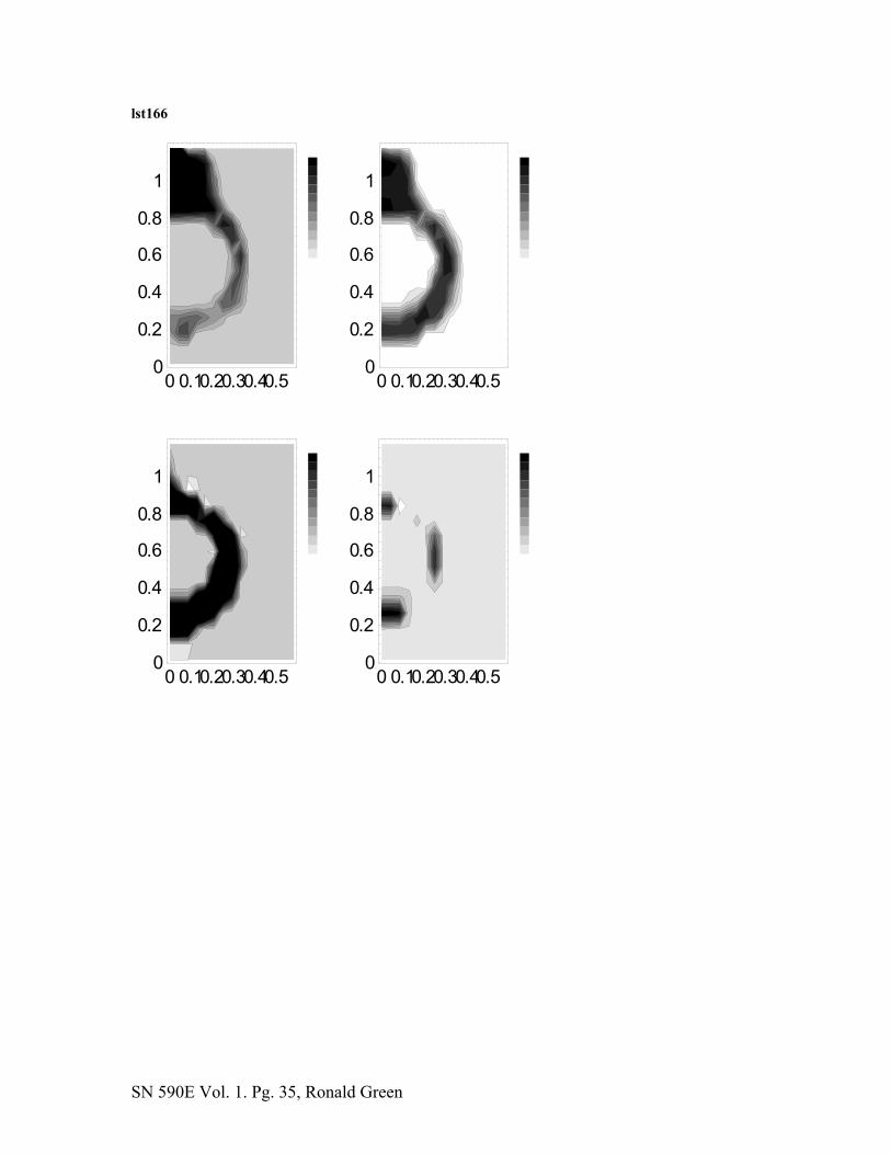
SN 590E Vol. 1. Pg. 35, Ronald Green
lst166
0 0.10.20.30.40.50
0.2
0.4
0.6
0.8
1
0 0.10.20.30.40.50
0.2
0.4
0.6
0.8
1
0 0.10.20.30.40.50
0.2
0.4
0.6
0.8
1
0 0.10.20.30.40.50
0.2
0.4
0.6
0.8
1

SN 590E Vol. 1. Pg. 36, Ronald Green
lst167
0 0.10.20.30.40.50
0.2
0.4
0.6
0.8
1
0 0.10.20.30.40.50
0.2
0.4
0.6
0.8
1
0 0.10.20.30.40.50
0.2
0.4
0.6
0.8
1
0 0.10.20.30.40.50
0.2
0.4
0.6
0.8
1

SN 590E Vol. 1. Pg. 37, Ronald Green
lst168
0 0.10.20.30.40.50
0.2
0.4
0.6
0.8
1
0 0.10.20.30.40.50
0.2
0.4
0.6
0.8
1
0 0.10.20.30.40.50
0.2
0.4
0.6
0.8
1
0 0.10.20.30.40.50
0.2
0.4
0.6
0.8
1

SN 590E Vol. 1. Pg. 38, Ronald Green
lst169
0 0.10.20.30.40.50
0.2
0.4
0.6
0.8
1
0 0.10.20.30.40.50
0.2
0.4
0.6
0.8
1
0 0.10.20.30.40.50
0.2
0.4
0.6
0.8
1
0 0.10.20.30.40.50
0.2
0.4
0.6
0.8
1
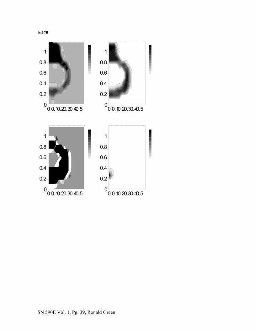
SN 590E Vol. 1. Pg. 39, Ronald Green
lst170
0 0.10.20.30.40.50
0.2
0.4
0.6
0.8
1
0 0.10.20.30.40.50
0.2
0.4
0.6
0.8
1
0 0.10.20.30.40.50
0.2
0.4
0.6
0.8
1
0 0.10.20.30.40.50
0.2
0.4
0.6
0.8
1

SN 590E Vol. 1. Pg. 40, Ronald Green
lst171
0 0.10.20.30.40.50
0.2
0.4
0.6
0.8
1
0 0.10.20.30.40.50
0.2
0.4
0.6
0.8
1
0 0.10.20.30.40.50
0.2
0.4
0.6
0.8
1
0 0.10.20.30.40.50
0.2
0.4
0.6
0.8
1

SN 590E Vol. 1. Pg. 41, Ronald Green
Lst172
0 0.10.20.30.40.50
0.2
0.4
0.6
0.8
1
0 0.10.20.30.40.50
0.2
0.4
0.6
0.8
1
0 0.10.20.30.40.50
0.2
0.4
0.6
0.8
1
0 0.10.20.30.40.50
0.2
0.4
0.6
0.8
1

SN 590E Vol. 1. Pg. 42, Ronald Green
Sensitivity analysis of the effect of matrix/fracture permeability changes Additional analyses are performed to evaluate the effect of changes in matrix and fracture permeability. Two sets of analyses are performed: one set varying matrix and fracture permeability for the lst155 basecase (simulations lst173-lst179). And one set (simulatons lst180-lst185) varying matrix and fracture permeability for the best match from the first set of analyses (lst160): AFM with 1.0 × 10⁻³ and γ = 0.4, 0.6, and 0.8. N/c denotes no convergence in simulation. Dec denotes that heat and mass transfer between the matrix and fracture continua are decoupled. Perm indicates whether the subject permeability is changed from the stated basecase. Flow denotes the presence of liquid flow features at the edge of the drift (i.e., shedding). Shed denotes whether there appears to be free (gravity-driven) flowing water at the edge of the drift. Pond denotes whether water is ponded above the drift. C Penet denotes whether there is evidence of downward flow penetrating into the drift (i.e., to what extent in the fracture below that to the side). Table 3. Summary of lst analyses: fracture Run No AFM γ α Perm Shed Sat Flow Pond C Penet lst173 Off - 1e-4 1.0 Yes 0.3054 Diffuse Yes lst174 Off - 1e-4 1.0 No 0.0460 Focused No No lst175 Off - 1e-4 -100x No 0.8505 Focused No No lst176 Off - 1e-4 +100x Yes 0.0260 Focused N/c No lst177 Off - 1e-4 1.0 No 0.0449 Focused No No lst178 Off - 1e-4 +10x Yes 0.0702 Focused N/c Some lst179 Off - 1e-5 1.0 Yes 0.2942 Focused No No lst180 On 0.4 1e-3 1.0 No 0.1457 Diffuse No lst181 On 0.4 1e-3 1.0 No 0.0000 None No No lst182 On 0.4 1e-3 -100x No 0.5571 Focused Some No lst183 On 0.4 1e-5 1.0 Yes 0.1792 Focused No Yes lst184 On 0.6 1e-4 1.0 Yes 0.1129 Focused Yes lst185 On 0.8 1e-4 1.0 Yes 0.0448 Focused No lst187 On 0.4 1e-3 1.0 No 0.0795 Focused No lst188 On 0.4 1e-3 1.0 No 0.0799 Focused No Table 4. Summary of lst analyses: matrix Run No AFM γ α Perm Sat CPond EPond MTem FTem lst173 Off - 1e-4 -10x 1.0000 Yes 179.8 179.3 lst174 Off - 1e-4 +10x 0.9183 No Some 187.5 187.0 lst175 Off - 1e-4 1.0 1.0000 No Some 187.4 186.9 lst176 Off - 1e-4 1.0 0.9945 No N/c 184.7 184.2 lst177 Off - 1e-4 1.0 0.4653 No Spme 188.3 187.8 lst178 Off - 1e-4 1.0 0.9954 No N/c 185.0 184.5 lst179 Off - 1e-5 1.0 0.9992 No Some 185.3 184.8 lst180 On 0.4 1e-3 -10x 1.0000 No 187.0 186.5 lst181 On 0.4 1e-3 +10x 0.8340 No Some 183.6 183.1 lst182 On 0.4 1e-3 1.0 1.0000 No Some 187.4 186.8

SN 590E Vol. 1. Pg. 43, Ronald Green
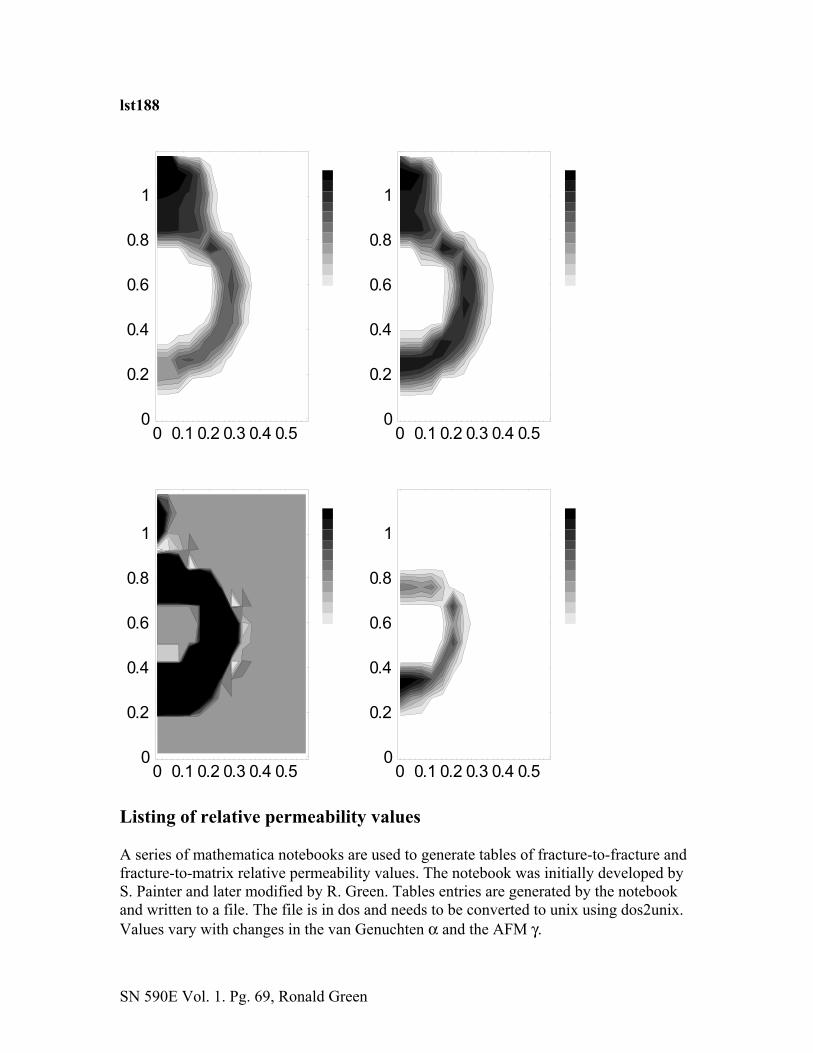
lst183 On 0.4 1e-5 1.0 0.9982 No Some 185.1 184.6 lst184 On 0.6 1e-4 1.0 0.9969 No 185.0 184.5 lst185 On 0.8 1e-4 1.0 0.9956 No 185.0 184.5 lst187 On 0.4 1e-3 1.0 0.9978 No 186.8 186.3 lst188 On 0.4 1e-3 1.0 0.9979 No 184.2 183.7 Discussion of analyses results. There are several main classes of analyses: 4) AFM 5) reduced areamodf, heat and mass coupled 6) reduced areamodf, heat and mass uncoupled Plus two sub-classes: 3) effect of alpha of 1e-3 versus 1e-4 4) effect of gamma=0.4 versus 0.6 and 0.8. Main observations: Inc matrix perm to 2e-16 (from 2e-17) in lst181 reduces fracture saturation to 0 for entire simulation. Inc matrix perm in non-AFM (lst174) does not have this profound effect, although fracture sat is relatively low. Lst173 and lst180 have shedding in fracture continua beyond end of drift. Both have reduced matrix perm from 2e-17 to 2e-18. Greatest smearing in fracture continuum occurred in lst173 and lst180, more in lst180. Fracture ponding above drift observed. No ponding (i.e., full saturation) observed in the matrix above the drift in all simulations. Higher than desirable saturation observed below the drift in all simulations. Lst 174, lst175, and lst181 have minimal flow in fracture continuum above middle of cell. Results from simulations lst173 through lst185, lst188 Following are graphs of 1) matrix saturation 2) matrix temperature 3) fracture saturation Matrix saturation – at center plane and at edge plane

SN 590E Vol. 1. Pg. 44, Ronald Green
lst173
0 0.1 0.2 0.3 0.4 0.50
0.2
0.4
0.6
0.8
1
0
1
0 0.1 0.2 0.3 0.4 0.50
0.2
0.4
0.6
0.8
1
0
1
lst174
0 0.1 0.2 0.3 0.4 0.50
0.2
0.4
0.6
0.8
1
0
1
0 0.1 0.2 0.3 0.4 0.50
0.2
0.4
0.6
0.8
1
0
1
lst175
0 0.1 0.2 0.3 0.4 0.50
0.2
0.4
0.6
0.8
1
0
1
0 0.1 0.2 0.3 0.4 0.50
0.2
0.4
0.6
0.8
1
0
1

SN 590E Vol. 1. Pg. 45, Ronald Green
lst176
0 0.1 0.2 0.3 0.4 0.50
0.2
0.4
0.6
0.8
1
0
1
0 0.1 0.2 0.3 0.4 0.50
0.2
0.4
0.6
0.8
1
0
1
lst177
0 0.1 0.2 0.3 0.4 0.50
0.2
0.4
0.6
0.8
1
0
1
0 0.1 0.2 0.3 0.4 0.50
0.2
0.4
0.6
0.8
1
0
1
lst178
0 0.1 0.2 0.3 0.4 0.50
0.2
0.4
0.6
0.8
1
0
1
0 0.1 0.2 0.3 0.4 0.50
0.2
0.4
0.6
0.8
1
0
1

SN 590E Vol. 1. Pg. 46, Ronald Green
lst179
0 0.1 0.2 0.3 0.4 0.50
0.2
0.4
0.6
0.8
1
0
1
0 0.1 0.2 0.3 0.4 0.50
0.2
0.4
0.6
0.8
1
0
1
lst180
0 0.1 0.2 0.3 0.4 0.50
0.2
0.4
0.6
0.8
1
0
1
0 0.1 0.2 0.3 0.4 0.50
0.2
0.4
0.6
0.8
1
0
1
lst181
0 0.1 0.2 0.3 0.4 0.50
0.2
0.4
0.6
0.8
1
0
1
0 0.1 0.2 0.3 0.4 0.50
0.2
0.4
0.6
0.8
1
0
1

SN 590E Vol. 1. Pg. 47, Ronald Green
lst182
0 0.1 0.2 0.3 0.4 0.50
0.2
0.4
0.6
0.8
1
0
1
0 0.1 0.2 0.3 0.4 0.50
0.2
0.4
0.6
0.8
1
0
1
lst183
0 0.1 0.2 0.3 0.4 0.50
0.2
0.4
0.6
0.8
1
0
1
0 0.1 0.2 0.3 0.4 0.50
0.2
0.4
0.6
0.8
1
0
1
lst184
0 0.1 0.2 0.3 0.4 0.50
0.2
0.4
0.6
0.8
1
0
1
0 0.1 0.2 0.3 0.4 0.50
0.2
0.4
0.6
0.8
1
0
1

SN 590E Vol. 1. Pg. 48, Ronald Green
lst185
0 0.1 0.2 0.3 0.4 0.50
0.2
0.4
0.6
0.8
1
0
1
0 0.1 0.2 0.3 0.4 0.50
0.2
0.4
0.6
0.8
1
0
1
lst187
0 0.1 0.2 0.3 0.4 0.50
0.2
0.4
0.6
0.8
1
0
1
0 0.1 0.2 0.3 0.4 0.50
0.2
0.4
0.6
0.8
1
0
1
lst188
0 0.1 0.2 0.3 0.4 0.50
0.2
0.4
0.6
0.8
1
0
1
0 0.1 0.2 0.3 0.4 0.50
0.2
0.4
0.6
0.8
1
0
1

SN 590E Vol. 1. Pg. 49, Ronald Green
Matrix temperature Temperatures range from 22 C (white) to the maximum (dark), as listed in Table 2 in this notebook. The left image is the xz plane. The right image is the yz plane. lst173
0 0.1 0.2 0.3 0.4 0.50
0.2
0.4
0.6
0.8
1
0.050.10.150.20.250
0.2
0.4
0.6
0.8
1
lst174
0 0.1 0.2 0.3 0.4 0.50
0.2
0.4
0.6
0.8
1
0.050.10.150.20.250
0.2
0.4
0.6
0.8
1

SN 590E Vol. 1. Pg. 50, Ronald Green
lst175
0 0.1 0.2 0.3 0.4 0.50
0.2
0.4
0.6
0.8
1
0.050.10.150.20.250
0.2
0.4
0.6
0.8
1
lst176
0 0.1 0.2 0.3 0.4 0.50
0.2
0.4
0.6
0.8
1
0.050.10.150.20.250
0.2
0.4
0.6
0.8
1
lst177
0 0.1 0.2 0.3 0.4 0.50
0.2
0.4
0.6
0.8
1
0.050.10.150.20.250
0.2
0.4
0.6
0.8
1

SN 590E Vol. 1. Pg. 51, Ronald Green
lst178
0 0.1 0.2 0.3 0.4 0.50
0.2
0.4
0.6
0.8
1
0.050.10.150.20.250
0.2
0.4
0.6
0.8
1
lst179
0 0.1 0.2 0.3 0.4 0.50
0.2
0.4
0.6
0.8
1
0.050.10.150.20.250
0.2
0.4
0.6
0.8
1
lst180
0 0.1 0.2 0.3 0.4 0.50
0.2
0.4
0.6
0.8
1
0.050.10.150.20.250
0.2
0.4
0.6
0.8
1

SN 590E Vol. 1. Pg. 52, Ronald Green
lst181
0 0.1 0.2 0.3 0.4 0.50
0.2
0.4
0.6
0.8
1
0.050.10.150.20.250
0.2
0.4
0.6
0.8
1
lst182
0 0.1 0.2 0.3 0.4 0.50
0.2
0.4
0.6
0.8
1
0.050.10.150.20.250
0.2
0.4
0.6
0.8
1
lst183
0 0.1 0.2 0.3 0.4 0.50
0.2
0.4
0.6
0.8
1
0.050.10.150.20.250
0.2
0.4
0.6
0.8
1

SN 590E Vol. 1. Pg. 53, Ronald Green
lst184
0 0.1 0.2 0.3 0.4 0.50
0.2
0.4
0.6
0.8
1
0.050.10.150.20.250
0.2
0.4
0.6
0.8
1
lst185
0 0.1 0.2 0.3 0.4 0.50
0.2
0.4
0.6
0.8
1
0.050.10.150.20.250
0.2
0.4
0.6
0.8
1
lst187
0 0.1 0.2 0.3 0.4 0.50
0.2
0.4
0.6
0.8
1
0.050.10.150.20.250
0.2
0.4
0.6
0.8
1

SN 590E Vol. 1. Pg. 54, Ronald Green
lst187
0 0.1 0.2 0.3 0.4 0.50
0.2
0.4
0.6
0.8
1
0.050.10.150.20.250
0.2
0.4
0.6
0.8
1
Fracture saturation Saturations range for 0 (white) to the maximum (see Table 1 in this notebook). There are four slices taken from each simulation. Of the ten slices provided in each mathematica notebook, slices 1, 5, 9, and 10 are copied to this scientific notebook.

SN 590E Vol. 1. Pg. 55, Ronald Green
lst173
0 0.1 0.2 0.3 0.4 0.50
0.2
0.4
0.6
0.8
1
0 0.1 0.2 0.3 0.4 0.50
0.2
0.4
0.6
0.8
1
0 0.1 0.2 0.3 0.4 0.50
0.2
0.4
0.6
0.8
1
0 0.1 0.2 0.3 0.4 0.50
0.2
0.4
0.6
0.8
1

SN 590E Vol. 1. Pg. 56, Ronald Green
lst174
0 0.1 0.2 0.3 0.4 0.50
0.2
0.4
0.6
0.8
1
0 0.1 0.2 0.3 0.4 0.50
0.2
0.4
0.6
0.8
1
0 0.1 0.2 0.3 0.4 0.50
0.2
0.4
0.6
0.8
1
0 0.1 0.2 0.3 0.4 0.50
0.2
0.4
0.6
0.8
1

SN 590E Vol. 1. Pg. 57, Ronald Green
lst175
0 0.10.20.30.40.50
0.2
0.4
0.6
0.8
1
0 0.10.20.30.40.50
0.2
0.4
0.6
0.8
1
0 0.10.20.30.40.50
0.2
0.4
0.6
0.8
1
0 0.10.20.30.40.50
0.2
0.4
0.6
0.8
1

SN 590E Vol. 1. Pg. 58, Ronald Green
lst176
0 0.1 0.2 0.3 0.4 0.50
0.2
0.4
0.6
0.8
1
0 0.1 0.2 0.3 0.4 0.50
0.2
0.4
0.6
0.8
1
0 0.1 0.2 0.3 0.4 0.50
0.2
0.4
0.6
0.8
1
0 0.1 0.2 0.3 0.4 0.50
0.2
0.4
0.6
0.8
1

SN 590E Vol. 1. Pg. 59, Ronald Green
lst177
0 0.10.20.30.40.50
0.2
0.4
0.6
0.8
1
0 0.10.20.30.40.50
0.2
0.4
0.6
0.8
1
0 0.10.20.30.40.50
0.2
0.4
0.6
0.8
1
0 0.10.20.30.40.50
0.2
0.4
0.6
0.8
1

SN 590E Vol. 1. Pg. 60, Ronald Green
lst178
0 0.1 0.2 0.3 0.4 0.50
0.2
0.4
0.6
0.8
1
0 0.1 0.2 0.3 0.4 0.50
0.2
0.4
0.6
0.8
1
0 0.1 0.2 0.3 0.4 0.50
0.2
0.4
0.6
0.8
1
0 0.1 0.2 0.3 0.4 0.50
0.2
0.4
0.6
0.8
1

SN 590E Vol. 1. Pg. 61, Ronald Green
lst179
0 0.10.20.30.40.50
0.2
0.4
0.6
0.8
1
0 0.10.20.30.40.50
0.2
0.4
0.6
0.8
1
0 0.10.20.30.40.50
0.2
0.4
0.6
0.8
1
0 0.10.20.30.40.50
0.2
0.4
0.6
0.8
1

SN 590E Vol. 1. Pg. 62, Ronald Green
lst180
0 0.1 0.2 0.3 0.4 0.50
0.2
0.4
0.6
0.8
1
0 0.1 0.2 0.3 0.4 0.50
0.2
0.4
0.6
0.8
1
0 0.1 0.2 0.3 0.4 0.50
0.2
0.4
0.6
0.8
1
0 0.1 0.2 0.3 0.4 0.50
0.2
0.4
0.6
0.8
1

SN 590E Vol. 1. Pg. 63, Ronald Green
lst181
0 0.1 0.2 0.3 0.4 0.50
0.2
0.4
0.6
0.8
1
0 0.1 0.2 0.3 0.4 0.50
0.2
0.4
0.6
0.8
1
0 0.1 0.2 0.3 0.4 0.50
0.2
0.4
0.6
0.8
1
0 0.1 0.2 0.3 0.4 0.50
0.2
0.4
0.6
0.8
1

SN 590E Vol. 1. Pg. 64, Ronald Green
lst182
0 0.1 0.2 0.3 0.4 0.50
0.2
0.4
0.6
0.8
1
0 0.1 0.2 0.3 0.4 0.50
0.2
0.4
0.6
0.8
1
0 0.1 0.2 0.3 0.4 0.50
0.2
0.4
0.6
0.8
1
0 0.1 0.2 0.3 0.4 0.50
0.2
0.4
0.6
0.8
1

SN 590E Vol. 1. Pg. 65, Ronald Green
lst183
0 0.1 0.2 0.3 0.4 0.50
0.2
0.4
0.6
0.8
1
0 0.1 0.2 0.3 0.4 0.50
0.2
0.4
0.6
0.8
1
0 0.1 0.2 0.3 0.4 0.50
0.2
0.4
0.6
0.8
1
0 0.1 0.2 0.3 0.4 0.50
0.2
0.4
0.6
0.8
1

SN 590E Vol. 1. Pg. 66, Ronald Green
lst184
0 0.1 0.2 0.3 0.4 0.50
0.2
0.4
0.6
0.8
1
0 0.1 0.2 0.3 0.4 0.50
0.2
0.4
0.6
0.8
1
0 0.1 0.2 0.3 0.4 0.50
0.2
0.4
0.6
0.8
1
0 0.1 0.2 0.3 0.4 0.50
0.2
0.4
0.6
0.8
1

SN 590E Vol. 1. Pg. 67, Ronald Green
lst185
0 0.1 0.2 0.3 0.4 0.50
0.2
0.4
0.6
0.8
1
0 0.1 0.2 0.3 0.4 0.50
0.2
0.4
0.6
0.8
1
0 0.1 0.2 0.3 0.4 0.50
0.2
0.4
0.6
0.8
1
0 0.1 0.2 0.3 0.4 0.50
0.2
0.4
0.6
0.8
1

SN 590E Vol. 1. Pg. 68, Ronald Green
lst187
0 0.10.20.30.40.50
0.2
0.4
0.6
0.8
1
0 0.10.20.30.40.50
0.2
0.4
0.6
0.8
1
0 0.10.20.30.40.50
0.2
0.4
0.6
0.8
1
0 0.10.20.30.40.50
0.2
0.4
0.6
0.8
1
SN 590E Vol. 1. Pg. 69, Ronald Green
lst188
0 0.1 0.2 0.3 0.4 0.50
0.2
0.4
0.6
0.8
1
0 0.1 0.2 0.3 0.4 0.50
0.2
0.4
0.6
0.8
1
0 0.1 0.2 0.3 0.4 0.50
0.2
0.4
0.6
0.8
1
0 0.1 0.2 0.3 0.4 0.50
0.2
0.4
0.6
0.8
1
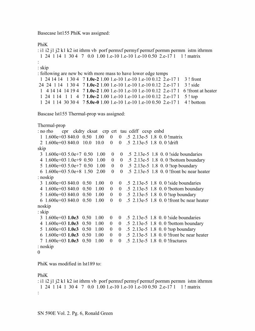
Listing of relative permeability values A series of mathematica notebooks are used to generate tables of fracture-to-fracture and fracture-to-matrix relative permeability values. The notebook was initially developed by S. Painter and later modified by R. Green. Tables entries are generated by the notebook and written to a file. The file is in dos and needs to be converted to unix using dos2unix. Values vary with changes in the van Genuchten α and the AFM γ.

SN 590E Vol. 1. Pg. 70, Ronald Green
Following is a plot of log relative permeability versus liquid saturation for different values of γ in the AFM. γ = 0.0 (solid), 0.2 (dotted), 0.4 (small dash), 0.6 (medium dash), and 0.8 (long dash).
0 0.2 0.4 0.6 0.8 1Liquid Saturation
1. ´ 10- 6
0.0001
0.01
1
goLevitaleR
ytilibaemreP
Table entries for relative permeability in Active Fracture Model Table 5. Fracture to fracture relative permeability Input file Mathematica nb Dos output Unix output γ α Lst180.dat AFM_lst_180 lst_ff180.dat ff180.dat 0.4 1e-3 Lst181.dat AFM_lst_180 lst_ff180.dat ff180.dat 0.4 1e-3 Lst182.dat AFM_lst_180 lst_ff180.dat ff180.dat 0.4 1e-3 Lst183.dat AFM_lst_183 lst_ff183.dat ff183.dat 0.4 1e-5 Lst184.dat AFM_lst_184 lst _ff184.dat ff184.dat 0.6 1e-4 Lst185.dat AFM_lst_185 lst _ff185.dat ff185.dat 0.8 1e-4 Lst187.dat AFM_lst_180 lst _ff180.dat ff180.dat 0.4 1e-3 Table 6. Fracture to matrix relative permeability Input file Mathematica nb Dos output Unix output γ α Lst180.dat AFM_lst_180 lst _fm180.dat fm180.dat 0.4 1e-3 Lst181.dat AFM_lst_180 lst _fm180.dat fm180.dat 0.4 1e-3 Lst182.dat AFM_lst_180 lst _fm180.dat fm180.dat 0.4 1e-3 Lst183.dat AFM_lst_183 lst_fm183.dat fm183.dat 0.4 1e-5 Lst184.dat AFM_lst_184 lst _fm184.dat fm184.dat 0.6 1e-4 Lst185.dat AFM_lst_185 lst _fm185.dat fm185.dat 0.8 1e-4 Lst187.dat AFM_lst_180 lst _fm180.dat fm180.dat 0.4 1e-3

This notebook was completed on September 5,2003
SM 590E Vol. 1. Pg. 71, Ronald Green

SN 590E Vol. 2. Pg. 1, Ronald Green
SCIENTIFIC NOTEBOOK E590
Volume 2
by
Ronald Green
Southwest Research Institute Center for Nuclear Waste Regulatory Analyses
San Antonio, Texas
September 9, 2003

SN 590E Vol. 2. Pg. 2, Ronald Green
Table of Contents INITIAL ENTRIES: Continuation of the laboratory-scale heater test (lst) analyses .................... 2 LST Thermal Boundary Conditions Analyses…………………………….………..........3 Table 1. Description of simulations, lst189 through lst196………………………………4 Table 2. Summary of results, lst189 through lst196............................................................7 Section 2: Analysis of heat transfer measurements on Tptpll

SN 590E Vol. 2. Pg. 3, Ronald Green
INITIAL ENTRIES
Scientific notebook: #590E Vol. 2 Issued to: R.T. Green Issue Date: 21-May-2003, Continued on September 9, 2003 as Volume 2
A series of MULTIFLO simulations are performed to examine data collected during the two lab-scale heater tests described in Scientific Notebook 209. Additional analyses are documented in e-Notebook 590 Vol 1. This notebook contains continued documentation of those analyses. All simulations were performed with MULTIFLO Version 1.5.2 August 2002.
LST THERMAL BOUNDARY CONDITIONS ANALYSES The first task documented in this notebook is to re-evlaute the thermal boundary conditions assigned to the lab-scale heater test. Following is a summary of theses simulation analyses performed using MULTIFLO. These simulation results will be compared with measured temperatures from Test 1 and Test 2 laboratory scale tests. Following are the measured temperatures at days 5, 50, and 110 during Test 1. These results were plotted using Surfer Version 8.03.

SN 590E Vol. 2. Pg. 4, Ronald Green
0.1 0.2 0.3
Width (m)
Hei
ght (
m)
0.1 0.2 0.3
Width (m)0.1 0.2 0.3
Width (m)
0.1
0.2
0.3
0.4
0.5
0.6
0.7
0.8
0.9
1.0
1.1
1.2
5 days 50 days 110 days
Test 1 data are in sideplotdata.xls in D:\Personal\text\kti\papers\wrr\. Above are measured temperatures at days 5, 50, and 110 of Test 1. Maximum temperature is 201.5 C at day 5, 195.6 C at day 50, and 187.8 C at day 110. Following are measured temperatures at days 10, 50, and 175 of Test 2. Maximum temperature was 245.6 C at day 10, 243.6 C at day 50, and 185.2 C at day 175. The highest temperature at each time was attributed to touching the cartridge heater and omitted. These data are found in isotherm_side_m.xls in D:\Personal\text\kti\papers\wrr\. There are 68 thermocouples in this plan according to the *xls file.

SN 590E Vol. 2. Pg. 5, Ronald Green
0.1 0.2 0.3 0.4 0.5 0.6
Width (m)0.1 0.2 0.3 0.4 0.5 0.6
Width (m)
Hei
ght (
m)
0.1 0.2 0.3 0.4 0.5 0.6
Width (m)
1.2
1.1
1.0
0.9
0.8
0.7
0.6
0.5
0.4
0.3
0.2
0.1 10 days 50 days 175 days
Table 1. Summary of experimental results Test Day Measured temperature maximum minimum Test 1 10 201.5 31.0 Test 1 50 195.6 30.4 Test 1 110 187.8 30.0 Test 2 10 220.76 33.19 Test 2 50 205.15 30.98 Test 2 175 197.49 27.73 These simulation results are located in /net/spock/home/rgreen/multi/lst/ross-lst/boundary/*. Following are descriptions of the simulations. All were run as variants to the assigned basecase in lst155.dat. Table 2. Description of simulations for lst thermal boundary conditions analyses Filename Simulation descritpion Result Lst189 Dec volume of boundary elements No heat loss through boundary Lst190 Inc volume of boundary elements Extreme heat loss thru boundaryLst191 Set bc vol between lst155 and lst189 Lst192 bc vol to default, inc bc heat cap at e4, e5 Did not converge Lst193 bc vol to default, inc bc heat cap to 1e7 Lst194 bc vol to default, inc bc heat cap to 5e5 Lst195 bc vol to default, inc bc heat cap to 1e4 Did not converge Lst196 bc vol to default, inc bc heat cap to 1e5 Did not converge
SN 590E Vol. 2. Pg. 6, Ronald Green
Basecase lst155 PhiK was assigned: PhiK : i1 i2 j1 j2 k1 k2 ist ithrm vb porf permxf permyf permzf pormm permm istm ithrmm 1 24 1 14 1 30 4 7 0.0 1.00 1.e-10 1.e-10 1.e-10 0.50 2.e-17 1 1 ! matrix : : skip : following are new bc with more mass to have lower edge temps 1 24 14 14 1 30 4 7 1.0e-2 1.00 1.e-10 1.e-10 1.e-10 0.12 2.e-17 1 3 ! front 24 24 1 14 1 30 4 7 1.0e-2 1.00 1.e-10 1.e-10 1.e-10 0.12 2.e-17 1 3 ! side 1 4 14 14 14 19 4 7 1.0e-2 1.00 1.e-10 1.e-10 1.e-10 0.12 2.e-17 1 6 !front at heater 1 24 1 14 1 1 4 7 1.0e-2 1.00 1.e-10 1.e-10 1.e-10 0.12 2.e-17 1 5 ! top 1 24 1 14 30 30 4 7 5.0e-0 1.00 1.e-10 1.e-10 1.e-10 0.50 2.e-17 1 4 ! bottom Bascase lst155 Thermal-prop was assigned: Thermal-prop : no rho cpr ckdry cksat crp crt tau cdiff cexp enbd 1 1.600e+03 840.0 0.50 1.00 0 0 .5 2.13e-5 1.8 0. 0 !matrix 2 1.600e+03 840.0 10.0 10.0 0 0 .5 2.13e-5 1.8 0. 0 !drift skip 3 1.600e+03 5.0e+7 0.50 1.00 0 0 .5 2.13e-5 1.8 0. 0 !side boundaries 4 1.600e+03 1.0e+9 0.50 1.00 0 0 .5 2.13e-5 1.8 0. 0 !bottom boundary 5 1.600e+03 5.0e+7 0.50 1.00 0 0 .5 2.13e-5 1.8 0. 0 !top boundary 6 1.600e+03 5.0e+8 1.50 2.00 0 0 .5 2.13e-5 1.8 0. 0 !front bc near heater : noskip 3 1.600e+03 840.0 0.50 1.00 0 0 .5 2.13e-5 1.8 0. 0 !side boundaries 4 1.600e+03 840.0 0.50 1.00 0 0 .5 2.13e-5 1.8 0. 0 !bottom boundary 5 1.600e+03 840.0 0.50 1.00 0 0 .5 2.13e-5 1.8 0. 0 !top boundary 6 1.600e+03 840.0 0.50 1.00 0 0 .5 2.13e-5 1.8 0. 0 !front bc near heater noskip : skip 3 1.600e+03 1.0e3 0.50 1.00 0 0 .5 2.13e-5 1.8 0. 0 !side boundaries 4 1.600e+03 1.0e3 0.50 1.00 0 0 .5 2.13e-5 1.8 0. 0 !bottom boundary 5 1.600e+03 1.0e3 0.50 1.00 0 0 .5 2.13e-5 1.8 0. 0 !top boundary 6 1.600e+03 1.0e3 0.50 1.00 0 0 .5 2.13e-5 1.8 0. 0 !front bc near heater 7 1.600e+03 1.0e3 0.50 1.00 0 0 .5 2.13e-5 1.8 0. 0 !fractures : noskip 0 PhiK was modified in lst189 to: PhiK : i1 i2 j1 j2 k1 k2 ist ithrm vb porf permxf permyf permzf pormm permm istm ithrmm 1 24 1 14 1 30 4 7 0.0 1.00 1.e-10 1.e-10 1.e-10 0.50 2.e-17 1 1 ! matrix :

SN 590E Vol. 2. Pg. 7, Ronald Green
: skip : following are new bc with more mass to have lower edge temps 1 24 14 14 1 30 4 1.00 1.e-10 1.e-10 1.e-10 0.12 2.e-17 1 3 ! front 24 24 1 14 1 30 4 1.00 1.e-10 1.e-10 1.e-10 0.12 2.e-17 1 3 ! side 1 4 14 14 14 19 4 1.00 1.e-10 1.e-10 1.e-10 0.12 2.e-17 1 6 ! front atheater 1 24 1 14 1 1 4 1.00 1.e-10 1.e-10 1.e-10 0.12 2.e-17 1 5 ! top 1 24 1 14 30 30 4 1.00 1.e-10 1.e-10 1.e-10 0.50 2.e-17 1 4 ! bottom PhiK modified in lst190 to: PhiK : i1 i2 j1 j2 k1 k2 ist ithrm vb porf permxf permyf permzf pormm permm istm ithrmm 1 24 1 14 1 30 4 7 0.0 1.00 1.e-10 1.e-10 1.e-10 0.50 2.e-17 1 1 ! matrix : : skip : following are new bc with more mass to have lower edge temps 1 24 14 14 1 30 4 7 1.0e-0 1.00 1.e-10 1.e-10 1.e-10 0.12 2.e-17 1 3 ! front 24 24 1 14 1 30 4 7 1.0e-0 1.00 1.e-10 1.e-10 1.e-10 0.12 2.e-17 1 3 ! side 1 4 14 14 14 19 4 7 1.0e-0 1.00 1.e-10 1.e-10 1.e-10 0.12 2.e-17 1 6 ! front atheater 1 24 1 14 1 1 4 7 1.0e-0 1.00 1.e-10 1.e-10 1.e-10 0.12 2.e-17 1 5 ! top 1 24 1 14 30 30 4 7 5.0e-1 1.00 1.e-10 1.e-10 1.e-10 0.50 2.e-17 1 4 ! bottom PhiK modified in lst191 to: PhiK : i1 i2 j1 j2 k1 k2 ist ithrm vb porf permxf permyf permzf pormm permm istm ithrmm 1 24 1 14 1 30 4 7 0.0 1.00 1.e-10 1.e-10 1.e-10 0.50 2.e-17 1 1 ! matrix : : skip : following are new bc with more mass to have lower edge temps 1 24 14 14 1 30 4 7 1.0e-3 1.00 1.e-10 1.e-10 1.e-10 0.12 2.e-17 1 3 ! front 24 24 1 14 1 30 4 7 1.0e-3 1.00 1.e-10 1.e-10 1.e-10 0.12 2.e-17 1 3 ! side 1 4 14 14 14 19 4 7 1.0e-3 1.00 1.e-10 1.e-10 1.e-10 0.12 2.e-17 1 6 ! front atheater 1 24 1 14 1 1 4 7 1.0e-3 1.00 1.e-10 1.e-10 1.e-10 0.12 2.e-17 1 5 ! top 1 24 1 14 30 30 4 7 5.0e-2 1.00 1.e-10 1.e-10 1.e-10 0.50 2.e-17 1 4 ! bottom PhiK modified in lst192 to: PhiK : i1 i2 j1 j2 k1 k2 ist ithrm vb porf permxf permyf permzf pormm permm istm ithrmm 1 24 1 14 1 30 4 7 0.0 1.00 1.e-10 1.e-10 1.e-10 0.50 2.e-17 1 1 ! matrix : : skip : following are new bc with more mass to have lower edge temps 1 24 14 14 1 30 4 7 0. 1.00 1.e-10 1.e-10 1.e-10 0.12 2.e-17 1 3 ! front 24 24 1 14 1 30 4 7 0. 1.00 1.e-10 1.e-10 1.e-10 0.12 2.e-17 1 3 ! side

SN 590E Vol. 2. Pg. 8, Ronald Green
1 4 14 14 14 19 4 7 0. 1.00 1.e-10 1.e-10 1.e-10 0.12 2.e-17 1 6 ! front at heater 1 24 1 14 1 1 4 7 0. 1.00 1.e-10 1.e-10 1.e-10 0.12 2.e-17 1 5 ! top 1 24 1 14 30 30 4 7 0. 1.00 1.e-10 1.e-10 1.e-10 0.50 2.e-17 1 4 ! bottom and Therm-prop was modified in lst192 to: Thermal-prop : no rho cpr ckdry cksat crp crt tau cdiff cexp enbd 1 1.600e+03 840.0 0.50 1.00 0 0 .5 2.13e-5 1.8 0. 0 !matrix 2 1.600e+03 840.0 10.0 10.0 0 0 .5 2.13e-5 1.8 0. 0 !drift : skip 3 1.600e+03 5.0e+3 0.50 1.00 0 0 .5 2.13e-5 1.8 0. 0 !side boundaries 4 1.600e+03 1.0e+4 0.50 1.00 0 0 .5 2.13e-5 1.8 0. 0 !bottom boundary 5 1.600e+03 5.0e+3 0.50 1.00 0 0 .5 2.13e-5 1.8 0. 0 !top boundary 6 1.600e+03 5.0e+3 1.50 2.00 0 0 .5 2.13e-5 1.8 0. 0 !front bc near heater noskip skip 3 1.600e+03 840.0 0.50 1.00 0 0 .5 2.13e-5 1.8 0. 0 !side boundaries 4 1.600e+03 840.0 0.50 1.00 0 0 .5 2.13e-5 1.8 0. 0 !bottom boundary 5 1.600e+03 840.0 0.50 1.00 0 0 .5 2.13e-5 1.8 0. 0 !top boundary 6 1.600e+03 840.0 0.50 1.00 0 0 .5 2.13e-5 1.8 0. 0 !front bc near heater : noskip : skip 3 1.600e+03 1.0e3 0.50 1.00 0 0 .5 2.13e-5 1.8 0. 0 !side boundaries 4 1.600e+03 1.0e3 0.50 1.00 0 0 .5 2.13e-5 1.8 0. 0 !bottom boundary 5 1.600e+03 1.0e3 0.50 1.00 0 0 .5 2.13e-5 1.8 0. 0 !top boundary 6 1.600e+03 1.0e3 0.50 1.00 0 0 .5 2.13e-5 1.8 0. 0 !front bc near heater noskip 7 1.600e+03 1.0e3 0.50 1.00 0 0 .5 2.13e-5 1.8 0. 0 !fractures : noskip 0 Therm-prop was modified in lst193 to: (lst193 PhiK same as lst192) Thermal-prop : no rho cpr ckdry cksat crp crt tau cdiff cexp enbd 1 1.600e+03 840.0 0.50 1.00 0 0 .5 2.13e-5 1.8 0. 0 !matrix 2 1.600e+03 840.0 10.0 10.0 0 0 .5 2.13e-5 1.8 0. 0 !drift : skip 3 1.600e+03 5.0e+7 0.50 1.00 0 0 .5 2.13e-5 1.8 0. 0 !side boundaries 4 1.600e+03 5.0e+7 0.50 1.00 0 0 .5 2.13e-5 1.8 0. 0 !bottom boundary 5 1.600e+03 5.0e+7 0.50 1.00 0 0 .5 2.13e-5 1.8 0. 0 !top boundary 6 1.600e+03 5.0e+7 0.50 1.00 0 0 .5 2.13e-5 1.8 0. 0 !front bc near heater noskip skip 3 1.600e+03 840.0 0.50 1.00 0 0 .5 2.13e-5 1.8 0. 0 !side boundaries

SN 590E Vol. 2. Pg. 9, Ronald Green
4 1.600e+03 840.0 0.50 1.00 0 0 .5 2.13e-5 1.8 0. 0 !bottom boundary 5 1.600e+03 840.0 0.50 1.00 0 0 .5 2.13e-5 1.8 0. 0 !top boundary 6 1.600e+03 840.0 0.50 1.00 0 0 .5 2.13e-5 1.8 0. 0 !front bc near heater : noskip : skip 3 1.600e+03 1.0e3 0.50 1.00 0 0 .5 2.13e-5 1.8 0. 0 !side boundaries 4 1.600e+03 1.0e3 0.50 1.00 0 0 .5 2.13e-5 1.8 0. 0 !bottom boundary 5 1.600e+03 1.0e3 0.50 1.00 0 0 .5 2.13e-5 1.8 0. 0 !top boundary 6 1.600e+03 1.0e3 0.50 1.00 0 0 .5 2.13e-5 1.8 0. 0 !front bc near heater noskip 7 1.600e+03 1.0e3 0.50 1.00 0 0 .5 2.13e-5 1.8 0. 0 !fractures : noskip 0 Therm-prop was modified in lst194 to: (lst194 PhiK same as lst192) Thermal-prop : no rho cpr ckdry cksat crp crt tau cdiff cexp enbd 1 1.600e+03 840.0 0.50 1.00 0 0 .5 2.13e-5 1.8 0. 0 !matrix 2 1.600e+03 840.0 10.0 10.0 0 0 .5 2.13e-5 1.8 0. 0 !drift : skip 3 1.600e+03 5.0e+5 0.50 1.00 0 0 .5 2.13e-5 1.8 0. 0 !side boundaries 4 1.600e+03 5.0e+5 0.50 1.00 0 0 .5 2.13e-5 1.8 0. 0 !bottom boundary 5 1.600e+03 5.0e+5 0.50 1.00 0 0 .5 2.13e-5 1.8 0. 0 !top boundary 6 1.600e+03 5.0e+5 0.50 1.00 0 0 .5 2.13e-5 1.8 0. 0 !front bc near heater noskip skip 3 1.600e+03 840.0 0.50 1.00 0 0 .5 2.13e-5 1.8 0. 0 !side boundaries 4 1.600e+03 840.0 0.50 1.00 0 0 .5 2.13e-5 1.8 0. 0 !bottom boundary 5 1.600e+03 840.0 0.50 1.00 0 0 .5 2.13e-5 1.8 0. 0 !top boundary 6 1.600e+03 840.0 0.50 1.00 0 0 .5 2.13e-5 1.8 0. 0 !front bc near heater : noskip : skip 3 1.600e+03 1.0e3 0.50 1.00 0 0 .5 2.13e-5 1.8 0. 0 !side boundaries 4 1.600e+03 1.0e3 0.50 1.00 0 0 .5 2.13e-5 1.8 0. 0 !bottom boundary 5 1.600e+03 1.0e3 0.50 1.00 0 0 .5 2.13e-5 1.8 0. 0 !top boundary 6 1.600e+03 1.0e3 0.50 1.00 0 0 .5 2.13e-5 1.8 0. 0 !front bc near heater noskip 7 1.600e+03 1.0e3 0.50 1.00 0 0 .5 2.13e-5 1.8 0. 0 !fractures : noskip 0 Therm-prop was modified in lst195 to: (lst195 PhiK same as lst192) Thermal-prop : no rho cpr ckdry cksat crp crt tau cdiff cexp enbd 1 1.600e+03 840.0 0.50 1.00 0 0 .5 2.13e-5 1.8 0. 0 !matrix 2 1.600e+03 840.0 10.0 10.0 0 0 .5 2.13e-5 1.8 0. 0 !drift

SN 590E Vol. 2. Pg. 10, Ronald Green
: skip 3 1.600e+03 5.0e+4 0.50 1.00 0 0 .5 2.13e-5 1.8 0. 0 !side boundaries 4 1.600e+03 5.0e+4 0.50 1.00 0 0 .5 2.13e-5 1.8 0. 0 !bottom boundary 5 1.600e+03 5.0e+4 0.50 1.00 0 0 .5 2.13e-5 1.8 0. 0 !top boundary 6 1.600e+03 5.0e+4 0.50 1.00 0 0 .5 2.13e-5 1.8 0. 0 !front bc near heater noskip skip Therm-prop was modified in lst196 to: (lst196 PhiK same as lst192 Thermal-prop : no rho cpr ckdry cksat crp crt tau cdiff cexp enbd 1 1.600e+03 840.0 0.50 1.00 0 0 .5 2.13e-5 1.8 0. 0 !matrix 2 1.600e+03 840.0 10.0 10.0 0 0 .5 2.13e-5 1.8 0. 0 !drift : skip 3 1.600e+03 1.0e+5 0.50 1.00 0 0 .5 2.13e-5 1.8 0. 0 !side boundaries 4 1.600e+03 1.0e+5 0.50 1.00 0 0 .5 2.13e-5 1.8 0. 0 !bottom boundary 5 1.600e+03 1.0e+5 0.50 1.00 0 0 .5 2.13e-5 1.8 0. 0 !top boundary 6 1.600e+03 1.0e+5 0.50 1.00 0 0 .5 2.13e-5 1.8 0. 0 !front bc near heater noskip skip Table 2. Summary of results for runs that converged Filename Matrix temp Matrix sat Fracture temp Fracture sat max min max min max min max min Lst155 185.1 20.01 0.9982 0.0 184.6 20.01 0.1792 0.0 Lst189 328.5 40.42 0.2203 0.0 328.0 40.42 0.0 0.0 Lst190 128.5 20.0 0.4179 0.0 127.9 20.0 0.0 0.0 Lst191 266.0 31.58 0.9359 0.0 265.4 31.58 0.0846 0.0 Lst193 120.4 20.0 1.0 0.0 119.9 20.0 0.7829 0.0 Lst194 194.5 48.11 0.999 0.0 193.9 48.12 0.7129 0.0
Simulated matrix temperature: Basecase Lst155

SN 590E Vol. 2. Pg. 11, Ronald Green
0 0.1 0.2 0.3 0.4 0.5
0
0.2
0.4
0.6
0.8
1
0.050.10.150.20.250
0.2
0.4
0.6
0.8
1
maximum matrix temp: 185.1 Lst189
0 0.1 0.2 0.3 0.4 0.50
0.2
0.4
0.6
0.8
1
0.050.10.150.20.250
0.2
0.4
0.6
0.8
1
maximum matrix temp: 328.5 Lst190

SN 590E Vol. 2. Pg. 12, Ronald Green
0 0.1 0.2 0.3 0.4 0.50
0.2
0.4
0.6
0.8
1
0.050.10.150.20.250
0.2
0.4
0.6
0.8
1
maximum matrix temp: 128.5 Lst191
0 0.1 0.2 0.3 0.4 0.50
0.2
0.4
0.6
0.8
1
0.050.10.150.20.250
0.2
0.4
0.6
0.8
1
max matrix temp: 266.0 Lst193
0 0.1 0.2 0.3 0.4 0.50
0.2
0.4
0.6
0.8
1
0.050.10.150.20.250
0.2
0.4
0.6
0.8
1
max matrix temp: 120.4

SN 590E Vol. 2. Pg. 13, Ronald Green
Lst194
0 0.1 0.2 0.3 0.4 0.50
0.2
0.4
0.6
0.8
1
0.050.10.150.20.250
0.2
0.4
0.6
0.8
1
maximum matrix temp: 194.5 Matrix saturation Measured matrix saturation
- 0.5 - 0.4 - 0.3 - 0.2 - 0.1- 1
- 0.8
- 0.6
- 0.4
- 0.2
- 0.5 - 0.4 - 0.3 - 0.2 - 0.1- 1
- 0.8
- 0.6
- 0.4
- 0.2
Basecase Lst155
0 0.1 0.2 0.3 0.4 0.50
0.2
0.4
0.6
0.8
1
0
1
0 0.1 0.2 0.3 0.4 0.5
0
0.2
0.4
0.6
0.8
1
0
1

SN 590E Vol. 2. Pg. 14, Ronald Green
Lst189
0 0.1 0.2 0.3 0.4 0.50
0.2
0.4
0.6
0.8
1
0
1
0 0.1 0.2 0.3 0.4 0.5
0
0.2
0.4
0.6
0.8
1
0
1
Lst190
0 0.1 0.2 0.3 0.4 0.50
0.2
0.4
0.6
0.8
1
0
1
0 0.1 0.2 0.3 0.4 0.5
0
0.2
0.4
0.6
0.8
1
0
1
Lst191
0 0.1 0.2 0.3 0.4 0.50
0.2
0.4
0.6
0.8
1
0
1
0 0.1 0.2 0.3 0.4 0.5
0
0.2
0.4
0.6
0.8
1
0
1
Lst193

SN 590E Vol. 2. Pg. 15, Ronald Green
0 0.1 0.2 0.3 0.4 0.50
0.2
0.4
0.6
0.8
1
0
1
0 0.1 0.2 0.3 0.4 0.5
0
0.2
0.4
0.6
0.8
1
0
1
Lst194
0 0.1 0.2 0.3 0.4 0.50
0.2
0.4
0.6
0.8
1
0
1
0 0.1 0.2 0.3 0.4 0.5
0
0.2
0.4
0.6
0.8
1
0
1
Fracture saturation Basecase Lst155
0 0.10.20.30.40.50
0.2
0.4
0.6
0.8
1
0 0.10.20.30.40.5
0
0.2
0.4
0.6
0.8
1
0 0.10.20.30.40.5
0
0.2
0.4
0.6
0.8
1
0 0.10.20.30.40.5
0
0.2
0.4
0.6
0.8
1
Lst189 (all fractures are at 0.0 saturation)

SN 590E Vol. 2. Pg. 16, Ronald Green
0 0.10.20.30.40.50
0.2
0.4
0.6
0.8
1
Lst190 (all fractures are at 0.0 saturation)
0 0.1 0.2 0.3 0.4 0.50
0.2
0.4
0.6
0.8
1
Lst191
0 0.1 0.2 0.3 0.4 0.50
0.2
0.4
0.6
0.8
1
0 0.1 0.2 0.3 0.4 0.50
0.2
0.4
0.6
0.8
1
0 0.1 0.2 0.3 0.4 0.50
0.2
0.4
0.6
0.8
1
0 0.1 0.2 0.3 0.4 0.50
0.2
0.4
0.6
0.8
1
Lst193
0 0.1 0.2 0.3 0.4 0.50
0.2
0.4
0.6
0.8
1
0 0.1 0.2 0.3 0.4 0.50
0.2
0.4
0.6
0.8
1
0 0.1 0.2 0.3 0.4 0.50
0.2
0.4
0.6
0.8
1
0 0.1 0.2 0.3 0.4 0.50
0.2
0.4
0.6
0.8
1
Based on these analyses, the basecase Lst155 has the best thermal boundary conditions. Re-ran basecase with revised upper and lower boundary conditions. The lower is gravity drainage. The upper is at atmospheric pressure.
SN 590E Vol. 2. Pg. 17, Ronald Green
lst202, inc int temp to 30 from 20 C lst204, inc source by scale = 1.4 lst205, inc by heat and mass in source by 1.4 lst206, inc mass in source by 1.7, heat inc by 1.4 lst207, inc mass in source by 2.0, heat inc by 1.4 lst208, dec matrix perm to 2e-18, same source as lst207 lst209, inc matrix perm to 2e-16, same source as lst207 lst210, set γ=0.8, α=1e-4, same source as lst207 Table x. Experimental and simulation results at 10 days Filename Matrix temp Matrix sat Fracture temp Fracture sat max min max min max min max min Test 1 201.5 31.0 Test 2 220.76 33.19 Lst155 130.9 20.00 0.4881 0.0 130.4 20.00 0.0536 0.0 Lst202 142.6 20.66 0.9931 0.0 142.0 20.66 0.0482 0.0 Lst204 190.6 20.71 0.9924 0.0 189.8 20.71 0.0543 0.0 Lst205 190.6 20.71 1.0 0.0 189.9 20.71 0.1090 0.0 Lst206 190.4 20.71 1.0 0.0 189.6 20.71 0.2450 0.0 Lst207 189.4 20.72 1.0 0.0 188.7 20.71 0.3066 0.0 Lst208 175.5 20.72 1.0 0.0 174.8 20.72 0.8500 0.0 Lst209 190.2 20.72 0.8471 0.0 189.4 20.71 0.0446 0.0 Lst210 176.7 20.67 1.0 0.0 176.0 20.66 0.3104 0.0 Table x. Experimental and simulation results at 50 days Filename Matrix temp Matrix sat Fracture temp Fracture sat max min max min max min max min Test 1 195.6 30.4 Test 2 240.04 31.5 Lst155 154.1 20.00 0.9470 0.0 154.3 20.00 0.0330 0.0 Lst202 164.6 20.62 0.9942 0.0 164.0 20.61 0.0480 0.0 Lst204 221.3 20.69 0.9932 0.0 220.5 20.68 0.0476 0.0 Lst205 221.1 20.68 1.0 0.0 220.3 20.68 0.1178 0.0 Lst206 219.6 20.69 1.0 0.0 218.9 20.69 0.2452 0.0 Lst207 216.6 20.69 1.0 0.0 215.9 20.69 0.3049 0.0 Lst208 192.4 20.70 1.0 0.0 191.7 20.70 0.5976 0.0 Lst209 219.4 20.69 0.8458 0.0 218.7 20.69 0.0444 0.0 Lst210 196.4 20.63 1.0 0.0 195.7 20.63 0.1366 0.0 Table x. Experimental and simulation results at 110 days Filename Matrix temp Matrix sat Fracture temp Fracture sat max min max min max min max min Test 1 187.8 30.0 Test 2 205.15 30.98 Lst155 171.1 20.00 1.0 0.0 171.1 20.00 0.3641 0.0

SN 590E Vol. 2. Pg. 18, Ronald Green
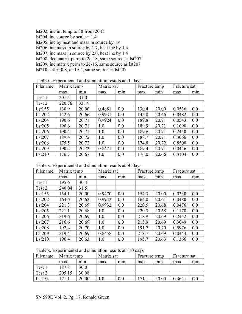
Lst202 179.5 20.63 0.9934 0.0 179.0 20.63 0.0510 0.0 Lst204 242.2 20.77 0.9916 0.0 241.6 20.77 0.0734 0.0 Lst205 242.0 20.77 0.9999 0.0 241.2 20.77 0.0769 0.0 Lst206 240.5 20.77 1.0 0.0 239.8 20.77 0.2282 0.0 Lst207 237.5 20.78 1.0 0.0 236.7 20.78 0.2927 0.0 Lst208 211.4 20.8 1.0 0.0 210.6 20.8 0.4045 0.0 Lst209 240.8 20.77 0.8414 0.0 240.0 20.77 0.0440 0.0 Lst210 213.4 20.68 1.000 0.0 212.6 20.68 0.1300 0.0 Table x. Experimental and simulation results at 175 days Filename Matrix temp Matrix sat Fracture temp Fracture sat max min max min max min max min Test 2 197.49 27.73 Lst155 178.4 20.10 1.0 0.0 177.9 20.10 0.4189 0.0 Lst202 187.7 20.80 0.9926 0.0 187.2 20.80 0.0548 0.0 Lst204 255.1 21.05 0.9904 0.0 254.3 21.05 0.0768 0.0 Lst205 254.7 21.05 0.9998 0.0 253.9 21.05 0.0791 0.0 Lst206 242.0 20.77 0.9999 0.0 241.2 20.77 0.0769 0.0 Lst207 250.4 21.06 1.0 0.0 249.7 21.06 0.2835 0.0 Lst208 222.6 21.60 1.0 0.0 221.9 21.10 0.4007 0.0 Lst209 253.6 21.06 0.8384 0.0 252.9 21.06 0.0438 0.0 Lst210 223.1 20.92 1.0 0.0 222.3 20.92 0.1245 0.0 These results suggest that decreasing matrix permeability (as in lst208) results in lower temperature and slightly higher fracture saturations. Increasing matrix permeability (as in lst209) results in slightly higher temperatures, slightly lower matrix saturations, and much lower fracture saturations. The fracture saturations predicted for the lower matrix permeability (lst209) are too low to be possible. A matrix permeability of 2e-18 m^2 is therefore ruled out. Temperature for lst202 is as follows
SN 590E Vol. 2. Pg. 19, Ronald Green
0 0.1 0.2 0.3 0.4 0.50
0.2
0.4
0.6
0.8
1
0.050.10.150.20.250
0.2
0.4
0.6
0.8
1
Temperature for lst204 at 172 days is as follows
0 0.1 0.2 0.3 0.4 0.50
0.2
0.4
0.6
0.8
1
0.050.10.150.20.250
0.2
0.4
0.6
0.8
1
Matrix saturation for lst202 at day 172 is as follows

SN 590E Vol. 2. Pg. 20, Ronald Green
0 0.1 0.2 0.3 0.4 0.50
0.2
0.4
0.6
0.8
1
0
1
0 0.1 0.2 0.3 0.4 0.50
0.2
0.4
0.6
0.8
1
0
1
Matrix saturation for lst204 at day 172 is as follows
0 0.1 0.2 0.3 0.4 0.50
0.2
0.4
0.6
0.8
1
0
1
0 0.1 0.2 0.3 0.4 0.5
0
0.2
0.4
0.6
0.8
1
0
1
Saturations range for 0 (white) to the maximum (see Table 1 in this notebook). There are four slices taken from each simulation. Of the ten slices provided in each mathematica notebook, slices 1, 5, 9, and 10 are copied to this scientific notebook. Fracture saturation for lst202 at day 172 is as follows [new basecase for new BC]
00.10.20.30.40.50
0.2
0.4
0.6
0.8
1
00.10.20.30.40.50
0.2
0.4
0.6
0.8
1
00.10.20.30.40.50
0.2
0.4
0.6
0.8
1
00.10.20.30.40.50
0.2
0.4
0.6
0.8
1

SN 590E Vol. 2. Pg. 21, Ronald Green
Fracture saturation for lst204 at day 172 is as follows [0nly diff from lst202 is inc heat by 1.4]
0 0.1 0.2 0.3 0.4 0.50
0.2
0.4
0.6
0.8
1
0 0.1 0.2 0.3 0.4 0.5
0
0.2
0.4
0.6
0.8
1
0 0.1 0.2 0.3 0.4 0.5
0
0.2
0.4
0.6
0.8
1
0 0.1 0.2 0.3 0.4 0.5
0
0.2
0.4
0.6
0.8
1
Fracture saturation for lst207 at day 172 is as follows
0 0.1 0.2 0.3 0.4 0.50
0.2
0.4
0.6
0.8
1
0 0.1 0.2 0.3 0.4 0.5
0
0.2
0.4
0.6
0.8
1
0 0.1 0.2 0.3 0.4 0.5
0
0.2
0.4
0.6
0.8
1
0 0.1 0.2 0.3 0.4 0.5
0
0.2
0.4
0.6
0.8
1
Fracture saturation for lst208 at day 172 is as follows
0 0.1 0.2 0.3 0.4 0.50
0.2
0.4
0.6
0.8
1
0 0.1 0.2 0.3 0.4 0.5
0
0.2
0.4
0.6
0.8
1
0 0.1 0.2 0.3 0.4 0.5
0
0.2
0.4
0.6
0.8
1
0 0.1 0.2 0.3 0.4 0.5
0
0.2
0.4
0.6
0.8
1
Fracture saturation for lst209 at day 172 is as follows
0 0.1 0.2 0.3 0.4 0.50
0.2
0.4
0.6
0.8
1
0 0.1 0.2 0.3 0.4 0.5
0
0.2
0.4
0.6
0.8
1
0 0.1 0.2 0.3 0.4 0.5
0
0.2
0.4
0.6
0.8
1
0 0.1 0.2 0.3 0.4 0.5
0
0.2
0.4
0.6
0.8
1

SN 590E Vol. 2. Pg. 22, Ronald Green
Fracture saturation for lst210 at day 172 is as follows
0 0.1 0.2 0.3 0.4 0.50
0.2
0.4
0.6
0.8
1
0 0.1 0.2 0.3 0.4 0.5
0
0.2
0.4
0.6
0.8
1
0 0.1 0.2 0.3 0.4 0.5
0
0.2
0.4
0.6
0.8
1
0 0.1 0.2 0.3 0.4 0.5
0
0.2
0.4
0.6
0.8
1
This notebook was completed on October 4, 2004.
SN 590E Vol. 3. Pg. 1, Ronald Green
SCIENTIFIC NOTEBOOK E590
Volume 3
by
Ronald Green
Southwest Research Institute Center for Nuclear Waste Regulatory Analyses
San Antonio, Texas
January 3, 2005

SN 590E Vol. 3. Pg. 2, Ronald Green
Table of Contents INITIAL ENTRIES: Continuation of the laboratory-scale thermal conductivity test analyses .......................................................................................................................................... 3 ............................................................7 Appendix A mathematica notebook rayleigh.nb…………………………………10

SN 590E Vol. 3. Pg. 3, Ronald Green
INITIAL ENTRIES
Scientific notebook: #590E Vol. 3 Issued to: R.T. Green Issue Date: 21-May-2003, Continued on January 3, 2005 as Volume 3 This notebook contains a continuation of the analyses of heat transfer through Tptpll. The
body of the text will be converted into a paper or report. Calculations were consolidated into a excel spreadsheet:
Thermal_k_final_b.xls
and one mathematica notebook: rayleigh.nb
This notebook is copied and included as Appendix A for convenience. The original lab data are documented in Scientific Notebook 212. Although the data were collected in 2000, the data were not analyzed at that time because the DOE decided to not consider engineered backfill as a design option. The data were recently analyzed in light of the possibility for early drift collapse and rockfall in the Tptpll. This prospect highlighted the need to understand the mechanisms and properties of heat flow through rubble. The analyses associated with this study are being summarized into a paper that will be submitted to a journal.
The draft text and figures for the paper or report are attached on January 3, 2005 are attached as Appendix A as a wordperfect file: th-k-tptpll_d.txt
Information in rayleigh.nb includes 1. Calculation of the Rayleigh number for porous media with a width-to-height
aspect ratio of unity. 2. Calculation of the Rayleigh number for porous media with a width-to-height
aspect ratios of 1.,.9,.8,.7,.6,.5,.4,.3, .2,.15,.125, .1, 1/30. 3. Calculation of the Rayleigh number for an actual drift with collapse, at a variety
of aspect ratios. These values are plotted in excel spreadsheet Thermal_k_final_b.xls.
The abstract for a proposed journal article is as follows: Thermally induced rock stresses at the potential high-level nuclear waste (HLW) repository at Yucca Mountain, Nevada, can degrade the drifts, possibly causing rubble to fall onto the dripshield overlying the emplaced waste packages. Thermal-hydrological processes will be altered by changes in thermal conductivity, ventilation, radiation, and convection resulting from such rockfalls. The purpose of this investigation is to measure heat transfer through crushed rock samples of the Topopah Spring lower lithophysal unit at Yucca Mountain as an analog of the rubble and to identify the important heat and mass transfer mechanisms for the expected range of conditions. A laboratory apparatus was used to measure heat transfer through the crushed tuff for temperatures as high as 173ºC and thermal gradients as large as 995ºC/m. A thermal conductivity value of 0.4 W/m-K was derived from measurements made at low temperatures, low

SN 590E Vol. 3. Pg. 4, Ronald Green
thermal gradients, and low saturation. Heat transfer by radiation was determined to be negligible, even at elevated temperatures, using empirical relations developed for granular packed bed media. Convection was determined to be that portion of heat transfer not attributed to conduction and radiation. Convection was observed in the laboratory apparatus at temperature gradients in excess of 600ºC/m. Heat transfer by convection through a rubble pile in a HLW emplacement drift, however, are calculated to occur at the much lower temperature gradients expected at the proposed Yucca Mountain geologic repository using a Rayleigh number analysis predicated on rubble properties calculated during these experiments. The draft paper’s introduction and background are as follows: Thermally induced stress at emplacement drifts at the potential high-level nuclear waste (HLW) repository at Yucca Mountain has been shown to lead to drift degradation (Gute et al., 2003; Ofoegbu et al., 2004). Drift degradation will be manifested as rockfall into the drift, possibly onto the dripshield overlying the emplaced waste packages. The transfer of heat through the zone near the degraded emplacement drifts will be altered by changes in thermal conductivity, ventilation, radiation, and convection resulting from the rockfall. In particular, the rubble pile will alter the thermal-hydrological processes by acting as a thermal insulator in the zone between the heat source (i.e., HLW canister) and the intact host rock and will affect the movement of liquid as vapor or liquid by altering the gas and liquid permeability for this region. Determining the impact of rubble on the design of a geologic repository is made difficult because heat and mass transfer through the engineered barrier and a rubble pile is a complex and coupled process. Complicating this transfer process is a high level of uncertainty in assigning property values to the highly heterogeneous structure of a rubble pile. A significant portion of the potential repository at Yucca Mountain as currently designed is predominately placed in the lower lithophysal unit of the Topopah Springs (Tptpll). Recent laboratory testing of the Tptpll by Brodsky et al. (2003a) provided relevant thermal conductivity measurements of intact samples of the rock matrix. Similarly, Brodsky et al. (2003b) has initiated field-scale thermal conductivity measurements of the Tptpll at the Enhanced Characterization of the Repository Block (ECRB) Cross Drift at Yucca Mountain Exploratory Studies Facility (ESF) to account for volume-average thermal conductivity of the rock including lithophysae. These two studies provide valuable end points in the continuum of possible rock textures that could comprise emplacement drift rock collapse. This does not imply that these texture end points also represent extreme values of thermal conductivity. In fact, actual rockfall thermal conductivity values could vary outside the range of values bracketed by the laboratory- (Brodsky et al., 2003a) and field- (Brodsky et al., 2003b) scale measurements. Transient and steady-state methods are available for measuring thermophysical properties. Both classes of methods have strengths and weaknesses. Transient methods permit calculation of thermal diffusivity and require shorter heating periods than steady-state methods of thermophysical properties (Singh and Chaudhary, 1992). Conversely, steady-state methods allow unambiguous determination of thermal conductivity as compared to transient methods which usually require an independent determination or estimation of heat capacity in order to determine thermal conductivity from thermal diffusivity measurements. Because the heat transfer processes at a geologic repository are expected to vary slowly, transient thermal effects are assumed to be of secondary importance compared to identification of the specific mechanisms active in the transfer of heat through rockfall. Therefore, thermal conductivity (or effective thermal conductivity), and not heat capacity or thermal diffusivity, is the primary focus of this investigation. The purpose of this investigation is the assessment of the thermophysical properties of an analog rubble pile and identification of the important heat and mass transfer mechanisms anticipated to be active under quasi-steady-state conditions in rubble collapsed around HLW canisters for conditions expected at a potential geologic HLW repository. To accomplish this objective, a steady-state laboratory apparatus was used to directly measure bulk thermal conductivity of
SN 590E Vol. 3. Pg. 5, Ronald Green
crushed rock for a range of temperatures. The laboratory method used in these experiments closely paralleled the methodology developed by Green et al. (1997). Laboratory experiments and analyses were conducted to investigate the various heat transfer mechanisms that might be active in a rubble pile expected in emplacement drifts (Gute et al., 2003; Ofoegbu et al., 2004). Analyses were conducted to identify the range of thermal-physical conditions over which the various heat transfer mechanisms would be active. This information is used to analyze the effects of a rubble pile in emplacement drifts at the potential repository that experience rockfall.
Background Conduction, convection, and radiation can potentially contribute to the transfer of heat from HLW canisters emplaced in a geologic repository. The complexity of the heat and mass transfer system near the heat-generating canister is compounded because the mechanisms that transfer heat through the drift space can vary in both space and time. These mechanisms could remain constant under stable drift conditions or they could be significantly altered in the event that rockfall occurs causing the dripshield overlying the canisters to be buried in a rubble pile. Heat transfer mechanisms would change due to the rubble pile acting as an insulator and the alteration of the free air space available for heat transfer by radiation and convection. The individual contributions by conduction, convection, and radiation to total heat transfer through the rockfall can be determined if sufficient information is available. At relatively low temperatures, heat transfer through intact rock at the potential repository will probably occur by conduction only. Heat transfer mechanism such as convection and radiation are expected to contribute to the total heat flow only at high temperatures or high thermal gradients. For circumstances with limited information, an effective thermal conductivity value which represents all active heat transfer mechanisms can be assigned to the medium for a specified range of conditions (Kaviany, 1995). This approach, however, may violate Fourier's law of heat conduction which assumes a linear relationship between heat flux and temperature gradient. Nonetheless, assuming an effective thermal conductivity is oftentimes expedient and, in reality, the only viable option available. Heat transfer through rockfall at higher temperatures may be complicated if a heat pipe is encountered. Heat pipes are a highly efficient heat transfer mechanism in which coupled evaporation, condensation, latent-heat transfer, and capillary-driven return flow of liquid remove heat at higher rates than normally experienced by conduction and convection (Mills, 1995). A heat-transfer mechanism similar to a heat pipe may form in the fractured, porous media near a heat-generating HLW canister. In this mechanism, which is commonly referred to as counter current, the return flow of water is driven by gravity, rather than by capillary forces active in a heat pipe. The rock unit under consideration is the Tptpll. The texture and strength of the Tptpll will affect drift integrity and how the rock breaks after failure. For example, heat transfer through large pieces of brittle rock will differ from heat transfer through crushed rock with lithophysae and a large portion of powder and fine-grained material. Therefore, evaluation of heat transfer through rockfall that may occur at the potential HLW repository at Yucca Mountain is performed on the actual host rock, that is, the Tptpll. Actual heat transfer through a rubble pile will depend on the physical properties of the native rock (i.e., fragment size distribution and packing) and thermal-hydrological conditions (i.e., temperature, temperature gradient, and saturation) encountered. The fragment size distribution and packing expected in the rubble pile are expected to be comparable to the sample tested in this analysis because the test specimen is the from the Tptpll unit although some rubble pile fragments may be larger. The assumption of low saturations used in this analysis is considered appropriate because the rubble pile will likely have a low saturation due to long durations (i.e., 100’s to 1,000’s of years) of heating expected for the repository as currently designed (DOE,

SN 590E Vol. 3. Pg. 6, Ronald Green
2004). The low saturation of the specimen will also diminish the potential importance of heat transfer by a heat pipe. Appendix A: Draft of the paper is at thermalK_journal_3.doc Calculation of time required for steady state to be attained during heating. Following is the equation used to calculate the time needed to raise the initial cell temperature to the final steady state temperature.
( ) ( )t A
qT T T T
C Msteadystatebottom
finaltop
finalbottominitial
topinitial
p rock=−
+−⎡
⎣⎢⎢
⎤
⎦⎥⎥2 2
where:
A is the cross-sectional area of the test cell, 0.81 m2, Cp is specific heat, 840 J/kg-K, Mrock is the mass of the test medium, 165 kg, and q is the heat flux measured at the bottom boundary, 186.6 W/m2.
This calculation assumes that all heat flux entering the test volume measured at the bottom heat flux sensors remained in the test specimen. The actual times needed to attain steady state in the tests were somewhat greater than this estimate mostly due to the fact that heat was removed from the system at the upper boundary heat sink before the entire test specimen attained the final desired temperature distribution. Nonetheless, this estimate provided a first-order approximation of the time required to make a valid measurement. To calculate the time required to approximate steady-state conditions, a specific heat of 840 J/kg-K was assigned to the crushed Tptpll. The mass of the test medium was determined to be 165 kg. Although initial temperatures in the experiments were dependent on the final temperature of the preceding experiment, the maximum increase in temperature from one test to the next was no greater than the 55ºC difference observed between Tests 9 and 10. The heat flux at the bottom boundary was measured 186.6 W/m2 at during Test 10. The time for steady-state temperatures to be achieved was estimated to be about 9 hours (actually 9.2 hrs). During conduct of the tests, a minimum of 48 hours was allowed for each test to attain steady-state temperatures. In addition, all experiments were continued until both the lower and upper heat flux measurements became steady, a condition that was realized in all twelve tests. Therefore, the assumption of steady-state heat flux conditions was justified for all tests. March 25, 2005 Calculations for the convection fitting parameter The convection fitting parameter was calculated using equation (8) from a draft of the thermal conductivity paper:

SN 590E Vol. 3. Pg. 7, Ronald Green
q c T Tconv conv critical= − ∇ − ∇⎛
⎝⎜
⎞
⎠⎟*
54
54
This was modified to solve for c*conv.
− = ∇ − ∇⎛
⎝⎜
⎞
⎠⎟c q T Tconv conv critical
* /54
54
The critical temperature gradient is set at 2800. Plotting of the data are included in sheet 4 of the excel spreadsheet thermal_k_final_b. The convection fitting parameter has a value of -0.346 for Test 1. This outlier was removed from the consensus plot. Test 5 is slightly anomalously high at 0.0759.
Test No.
Qconv ∇T5/4 c*conv -2500
c*conv -2550
c*conv -2600
c*conv -2650
c*conv -2700
c*conv -2750
1 0.2295 0.3174 0.5147 1.3593 -2.1198 -0.59552 0.8 1378.2 -0.0007 -0.0007 -0.0007 -0.0006 -0.0006 -0.00063 -6.1 829.7 0.0037 0.0036 0.0035 0.0034 0.0033 0.00324 -3.5 2095.3 0.0087 0.0078 0.0070 0.0064 0.0059 0.00545 7.3 2895.9 0.0184 0.0211 0.0246 0.0296 0.0372 0.04996 29.9 4024.6 0.0196 0.0203 0.0210 0.0217 0.0225 0.02347 62.2 5112.3 0.0238 0.0243 0.0247 0.0253 0.0258 0.02638 -3.9 1243.3 0.0031 0.0030 0.0029 0.0028 0.0027 0.00269 -7.6 556.0 0.0039 0.0038 0.0037 0.0036 0.0035 0.003510 2.3 2275.2 -0.0101 -0.0083 -0.0070 -0.0061 -0.0054 -0.004811 23.2 3696.4 0.0194 0.0202 0.0212 0.0222 0.0233 0.024512 71.4 5590.2 0.0231 0.0235 0.0239 0.0243 0.0247 0.0251
Tests 2, 3, 4, 8, 9, and 10 are sufficiently close to 0 (i.e., ±0.007). Tests 5, 6, 7, 11, and 12 are all 0.021 to 0.025 for a critical threshold of 2600. The plot for this table is (not plotting for 2750 and omitting Test 1):

SN 590E Vol. 3. Pg. 8, Ronald Green
-0.020
-0.010
0.000
0.010
0.020
0.030
0.040
0 1000 2000 3000 4000 5000 6000
-2500-2550-2600-2650-2700
The critical threshold was selected from this graph. Values for the convection fitting parameter near the onset of convection are sensitive to the choice of the critical threshold. Values for the fitting parameter above and below the transition zone, however, are not sensitive to this selection. Data for a critical threshold of 2600 only are plotted on the following graph. Test 1 is an outlier and has been omitted.
-0.03
-0.02
-0.01
0.00
0.01
0.02
0.03
0 1000 2000 3000 4000 5000 6000
(Temperature Gradient)**5/4
Con
vect
ion
Fitt
ing
Para
met
er
This plot illustrates the onset of convection occurs at a temperature gradient**5/4 of about 2500-2700.

SN 590E Vol. 3. Pg. 9, Ronald Green
March 30, 2005 Slightly modified version of figure illustrating the convection fitting parameter as a function of (temperature gradient)**(5/4).
This version of the plot illustrates the onset of convection occurs at a slightly different temperature gradient**5/4 of about 1800-2600. April 22, 2005 This entry concludes SN 590E Vol 3, with the exception of the two page Appendix A, a printout of a mathematica notebook.
-0.03
-0.02
-0.01
0.00
0.01
0.02
0.03
0 1000 2000 3000 4000 5000 6000
(Temperature Gradient)**5/4
Con
vect
ion
Fitt
ing
Para
met
er
5/4
onset of convection

SN 590E Vol. 3. Pg. 10, Ronald Green
Appendix A: Printout of mathematica notebook rayleigh.nb Rayleigh Number Calculation (Ron Green 12/29/04) $Version 5.0 for Microsoft Windows (June 11, 2003) $DefaultFont={"Helvetica-Bold",18} big = {"Helvetica-Bold",18} Needs["Graphics`Graphics`"] Needs["Graphics`Colors`"] Off[General::spell1] {Helvetica-Bold,18} {Helvetica-Bold,18} AllColors; Critical Rayleigh number for width/height aspect ratio of unity perm = 1 10.^-3 cm^2; rho = 0.0012 g/cm^3; grav = 980.0 cm/sec^2; beta = 3. 10^-3 1/c; delt = 50. c; cv = 0.9 J/{g c}; dist = 15.0 cm; mu = 2. 10^-4 g/{cm sec}; xi = 0.4 10^-3 J/{cm c sec}; ra = perm*rho^2*grav*beta*delt*cv*dist/(mu*xi) {35.721} Critical Rayleigh number for width/height aspect ratio of less than unity (s=aspect ratio) from Donaldson (1970) s={1.,.9,.8,.7,.6,.5,.4,.3, .2,.15,.125, .1, 1/30.}; s={0.5,0.33333,0.25,.2,0.166666667,0.142857143,0.125}; factor = 1+(-1/2 + (1/2) (1 + 4 s^2)^(1/2)) m = IntegerPart [factor] m=1; ra = Pi^2 (m^2 + s^2)^2/(m^2 s^2) {1.20711,1.10092,1.05902,1.03852,1.02705,1.02001,1.01539} {1,1,1,1,1,1,1} {61.685,109.664,178.27,266.874,375.319,503.551,651.548} Calculate Rayleigh number for collapsed drift perm=1 10.^-3 cm^2; rho=0.0012 g/cm^3; grav=980.0 cm/sec^2; beta=3. 10^-3 1/c; delt=50. c; cv=0.9 J/{g c}; dist={ 3500. } cm; mu=2. 10^-4 g/{cm sec}; xi=0.4 10^-3 J/{cm c sec};

ra=perm*rhoA2*grav*beta*delt*cv*dist/(mu*xi) Calculate collapsed drift for number Rayleigh { 8 3 3 4 . 9 }
SN 590E Vol. 3 . Pg. 1 1, Ronald Green

SN 590E Vol. 4. Pg. 1, Ronald Green
SCIENTIFIC NOTEBOOK E590
Volume 4
by
Ronald Green
Southwest Research Institute Center for Nuclear Waste Regulatory Analyses
San Antonio, Texas
January 23, 2006

Table of Contents
INITIAL ENTRIES : Continuation of the laboratory-scale thermal conductivity test analyses 7 ; ........................................................................................................................................... - ............................................................
SN 590E Vol. 4. Pg. 2, Ronald Green

SN 590E Vol. 4. Pg. 3, Ronald Green
INITIAL ENTRIES
Scientific notebook: #590E Vol. 4 Issued to: R.T. Green Issue Date: 21-May-2003, Continued on January 23, 2006 as Volume 4
This notebook contains a continuation of the analyses of heat transfer through Tptpll. The title of the experiment and associated analyses is evaluation of heat flow through crushed Tptpll. Ron Green is the principal investigator and is responsible for data analysis. Jim Prikryl was responsible for the execution of the laboratory experiment. The experiment entailed the measurement of heat flow through a container filled with crushed Tptpll under different temperatures and different temperature gradients. Analyses are performed to determine what modes of heat transfer contributed to heat flow through the Tptpll sample, either by conduction, convection, or radiation. The mathematica notebook in SN #590E volume 3 contained the following: perm = 1 10.^-7 m^2; rho = 1.2 kg/m^3; grav = 9.80 m/sec^2; beta = 3. 10^-3 1/C; delt = 50. C; cv = 900.0 J/{kg C}; dist = 0.15 m; mu = 2. 10^-5 kg/{m sec}; xi = 0.4 10^-1 J/{m C sec}; ra = perm*rho^2*grav*beta*delt*cv*dist/(mu*xi) The critical value of Ra is 4π2 or 39.478. The permeability of coarse gravel is 1 x 10⁻⁷ m2 per Freeze and Cherry. Density of moist air is 1.225 kg/m3 Gravity is 9.80 m/sec2 Beta is the coefficient of volumetric expansion 3.67 x 10⁻³ C-1 for air.

SN 590E Vol. 4. Pg. 4, Ronald Green
Delta temperature is 50 C this value is approximate for the experiments, actual values ranged from 23.6 to 149.3 C. Cv is the specific heat at constant volume in J/kg C, this is 661 J/kg C for oxygen and 741 J/kg C for nitrogen at 25 C. For air, specific heat at constant volume: .715 Joules per gram per degree Kelvin or .17 BTU's per pound per degree Rankine. Taken from nasa website: http://www.grc.nasa.gov/WWW/Wright/airplane/airprop508.html Distance is 0.15 m from the experiment mu is (absolute or dynamic) viscosity of air 2 x 10⁻⁵ kg/m sec, from Fox and McDonald xi is effective thermal conductivity, measured at 0.4 J/(m C sec) or 0.4 W/(m C) Based on this summary, the value for thermal conductivity in the table above was low by a factor of 10. It should be 0.4 W/m K, not 0.04 W/m K. The value of Ra is decreased from 35.721 to 3.572. If the delta temperature is changed from 50 C to 149.3 C (as in test 12), then the Ra is 10.666. Dynamic viscosity at 150 C and standard pressure is approximately 2.38 10-5 kg/m sec, then Ra is 12.693. From chart taken from internet. If the density of air is changed from 1.2 to 1.225 kg/m3, then Ra is 12.957. This is still a factor of 3 below the critical Ra. It can be argued that coarse gravels have permeabilites as large as 10-6 m2. If so, this would push Ra above the critical value. Reference: Characterization of Hydraulic Properties of Potentially Fractured Industrial D Landfill Sites, and A Study of Heterogeneity Effects on Fate and Transport in Groundwater. US EPA National Risk Management Research Laboratory. Subsurface Protections and Remediations division. Ada, OK. 74820. March 1998. http://www.epa.gov/epaoswer/hazwaste/id/hwirwste/pdf/risk/reports/s0548.pdf also: API, 1989. Hydrogeologic Database for Groundwater Modeling. API Publication No. 4476, American Petroleum Institute. Or Newell, C.J., L.P. Hopkins, and P.B. Bedient. 1989. Hydrogeologic Database for Ground Water Modeling. API Publication No. 4476. American Petroleum Institute, Washington, DC. April 3, 2006 Another issue to resolve in the peer review of the Nuclear Technology journal article submittal is measurement error. An additional section was added. This section reads as follows:

‘The standard deviations of heat flux measurements, as illustrated by the outer error bars in Figure 4, are sufficiently large that they could conceivably account for the entire departure of measured heat flux from the pure conduction straight line in Figure 4. The standard deviation included in Figure 4 is interpreted to include instrument uncertainty and experiment variability. Instrument accuracy can be quantified using published absolute calibration accuracy values of 3 4 % for the Micro-FoilTM heat flux sensors (RdF Corporation, 2006). An inner set of error bars, based on 5%, are included in Figure 4.
The difference between the 5% measurement error bars and the larger observed standard deviation is attributed to experimental variability resulting mostly from non-uniform thermal contact between the metal heat exchangers and the irregularly sized and shaped rock fragments. The variability in heat flow measurement at the four heat flux sensors in the top and in the bottom are indicative of variability of heat flux measured at places where the thermal contact between the rock fragments and the heat exchanger was high, hence high heat flux, and places where the thermal contact between the rock fragments and the heat exchanger was low, hence low heat flux. Minimizing this variability was achieved, in part, by placing crumpled tin foil between the top of the rock and the top heat exchanger. This procedure was not used at the bottom where better thermal contact was believed to have been achieved during packing of the rock fragments in the test cell.
This assessment of experimental variability is supported by the fact that variability among heat sensor measurements exhibited clear trends: (i) variability was larger at higher temperatures and higher temperature gradients and (ii) the same heat flux sensors in the top and bottom consistently had the highest, and lowest, measured heat flux in all tests. The relative consistency of these measurements supports the premise that the experiment variation was due to differences in thermal contact between the heat flux sensors and the rock fragments and was not due to either significant non-linear heat flow through the rock fragments or random measurement error. Based on this reasoning, the
SN 590E Vol. 4. I’g. 5 , Ronald Green

average values for heat flux are believed to be valid and calculation of the non- conductivity cornponent of heat flux from the departure from the linear segment of the curve is also believed to be valid.
SN 590E Vol. 4. I’g. 6, Ronald Green


![Scientific Notebook No. 759E: Reliability of Passive ... · Fernando Ferrante SCIENTIFIC NOTEBOOK #759E INITIALS: FF [1] 1. INITIAL ENTRIES Scientific Note Book: # 759 Issued to:](https://img.pdfslide.us/doc/110x75/604fdb2a1fddad3a58323ed7/scientific-notebook-no-759e-reliability-of-passive-fernando-ferrante-scientific.jpg)