Science Seminar Presentation

Yana Kortsarts

Computer Science

Research in Computer Science Education

Integration of the mathematical reasoning into undergraduate computer science curriculum

Mathematical Reasoning (math-thinking discussion group: http://www.math-in-cs.org/)

Applying mathematical techniques, concepts, and processes, either explicitly or implicitly, in the solution of problems

In the most general interpretation, every problem-solving activity is an application of mathematical reasoning.

“Mathematics organizes and puts our mind in order.” Mikhail Lomonosov (1711-1765)

Enriching Introductory Programming Courses with Non-Intuitive Probability

Experiments Component ITiCSE 2012

17th Annual Conference on Innovation and Technology in Computer Science Education

Yana Kortsarts Computer Science Department, Widener University, Chester, PA

Yulia Kempner

Department of Computer Science, Holon Institute of Technology, Holon, Israel

Introduction

Probability theory is branch of mathematics that plays one of the central roles, not only in computer science, but also in science at large

The focus of the current work is on the integration of the non-intuitive probability experiments into the introductory programming course

We consider a set of the probability problems in which the intuitive approach leads to the wrong solution.

Introduction

These examples do not require any knowledge of probability The value of the probability or the expectation is computed

via a program that students run All material that these problems require is covered already

in the introductory programming course curriculum These problems are based on interesting scenarios, attractive

to students, and could be successfully “translated” into programming assignments.

We present and discuss numerical simulations and verification of the correct solution through the computational approach.

Goals and Objectives

The proposed enrichment helps to achieve the following goals: Engaging students in experimental problem

solving Increasing students’ motivation and interest in

programming Increasing students’ attention and curiosity

during the class Enhancing students’ programming skills

Non-Intuitive Testable Probabilities

Non-intuitiveness of many probability statements Difficult for students to guess a correct answer Non-intuitiveness: Intuitive problem solving leads

to the wrong answer Testability: The non-intuitive probability problem

could be “translated” into a programming assignment. It is possible to compute, or closely approximate, the required probability or expectation by writing a program with a low running time

The Averaging Principle

While designing a numerical simulation it is important to take into account that, given a single trial, the value reached can be far off the expectation

We apply the averaging principle The program simulates the experiment many times; the

results for all trials are added and then averaged at the end to obtain a final answer

By simple laws of probability of sum of independent events , we know that the average value, produced by our program, will converge to the correct result

Is your random number generator really random?

It is known that randomized algorithms might perform poorly because the random number generator was faulty

Checking the performance of the random number generator provides a soft introduction to the subject of estimating random events

An obvious remark is that we do not know how to find even a single random bit. Still, we do know how to create pseudo-random bits

Is your random number generator really random?

To evaluate the behavior of the random number generator, we ask students to consider the simple experiment of throwing a fair coin with ‘H’ and ‘T’ 1000000 times

This is a single trial of the experiment, and we ask students to verify that, for example, the number of resulting ‘H’s is about 500000.

For this example, it is known that standard deviation is

1000000,5004

nn

Classical problem: "Let's Make a Deal"

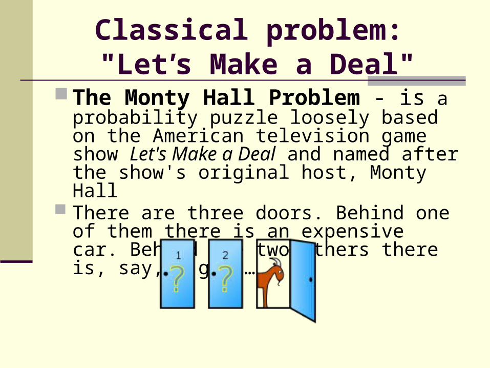
The Monty Hall Problem - is a probability puzzle loosely based on the American television game show Let's Make a Deal and named after the show's original host, Monty Hall

There are three doors. Behind one of them there is an expensive car. Behind the two others there is, say, a goat…

Experiment is conducted as follows:

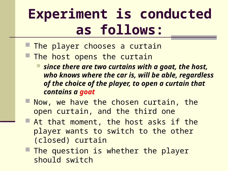
The player chooses a curtain The host opens the curtain

since there are two curtains with a goat, the host, who knows where the car is, will be able, regardless of the choice of the player, to open a curtain that contains a goat

Now, we have the chosen curtain, the open curtain, and the third one

At that moment, the host asks if the player wants to switch to the other (closed) curtain

The question is whether the player should switch

Intuitive Answer

For almost all students, since the chosen door and the other closed door look the same, the intuitive answer is

not to switch

Numerical Solution

def makeDeal(n):

doSwitch=0

noSwitch=0

for i in range(n):

carDoor=random.randint(1,3)

playerDoor=random.randint(1,3)

if(carDoor==playerDoor):

noSwitch+=1

else:

doSwitch+=1

return (float)(noSwitch)/n, (float)(doSwitch)/n

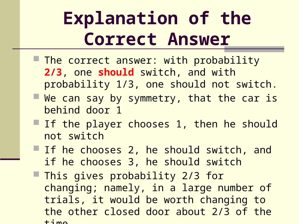
Explanation of the Correct Answer

The correct answer: with probability 2/3, one should switch, and with probability 1/3, one should not switch.

We can say by symmetry, that the car is behind door 1 If the player chooses 1, then he should not switch If he chooses 2, he should switch, and if he chooses 3, he

should switch This gives probability 2/3 for changing; namely, in a large

number of trials, it would be worth changing to the other closed door about 2/3 of the time

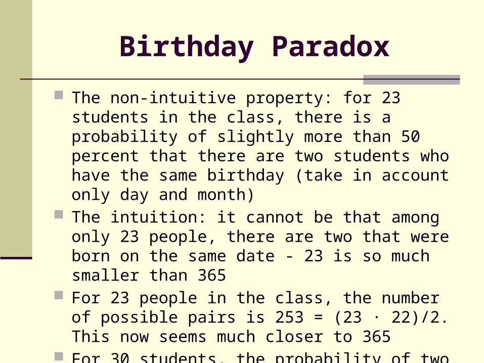
Birthday Paradox

The non-intuitive property: for 23 students in the class, there is a probability of slightly more than 50 percent that there are two students who have the same birthday (take in account only day and month)

The intuition: it cannot be that among only 23 people, there are two that were born on the same date - 23 is so much smaller than 365

For 23 people in the class, the number of possible pairs is 253 = (23 · 22)/2. This now seems much closer to 365

For 30 students, the probability of two people being born on the same day is 0.7

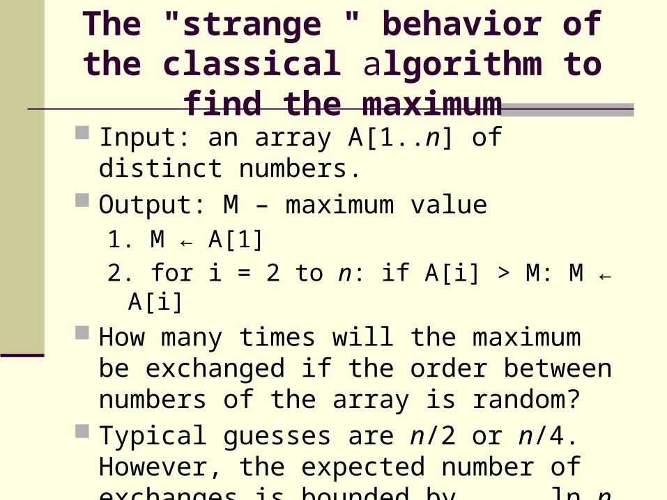
The "strange " behavior of the classical algorithm to find the maximum

Input: an array A[1..n] of distinct numbers. Output: M – maximum value

1. M ← A[1]

2. for i = 2 to n: if A[i] > M: M ← A[i] How many times will the maximum be exchanged

if the order between numbers of the array is random?

Typical guesses are n/2 or n/4. However, the expected number of exchanges is bounded by ln n + O(1)

Theoretical Explanation

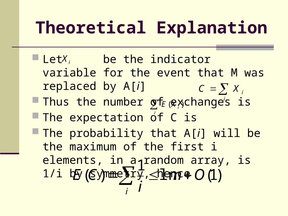
Let be the indicator variable for the event that M was replaced by A[i]

Thus the number of exchanges is The expectation of C is The probability that A[i] will be the maximum of

the first i elements, in a random array, is 1/i by symmetry, hence

i

iXC

i

iXE )(

iX

)1(ln1

)( Oni

CEi

Numerical Solution

Since only the order of the numbers is important, we recommend the use of numbers 1, 2, . . . , n as the entries of an array of size n

To generate a random permutation of the numbers 1, 2, . . . , n, we recommend using the Fisher-Yates shuffle, also known as the Knuth shuffle with time complexity O(n)

Fisher-Yates (Knuth) Shuffle

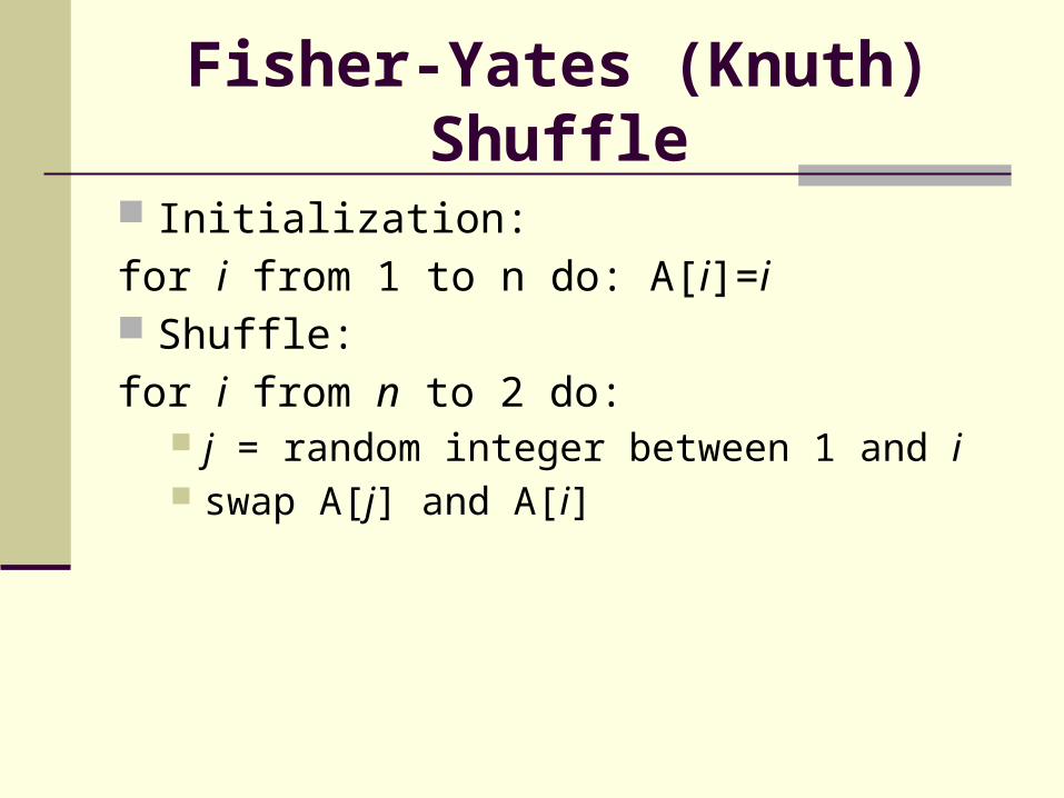
Initialization:

for i from 1 to n do: A[i]=i Shuffle:

for i from n to 2 do: j = random integer between 1 and i swap A[j] and A[i]

The strange behavior of random walks

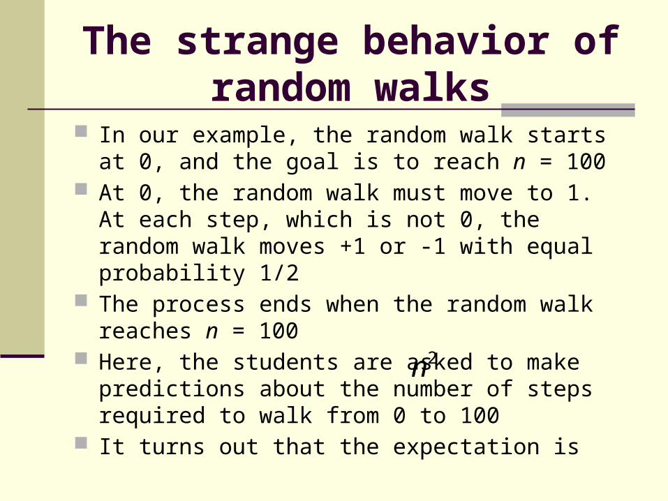
In our example, the random walk starts at 0, and the goal is to reach n = 100

At 0, the random walk must move to 1. At each step, which is not 0, the random walk moves +1 or -1 with equal probability 1/2

The process ends when the random walk reaches n = 100 Here, the students are asked to make predictions about the

number of steps required to walk from 0 to 100 It turns out that the expectation is 2n

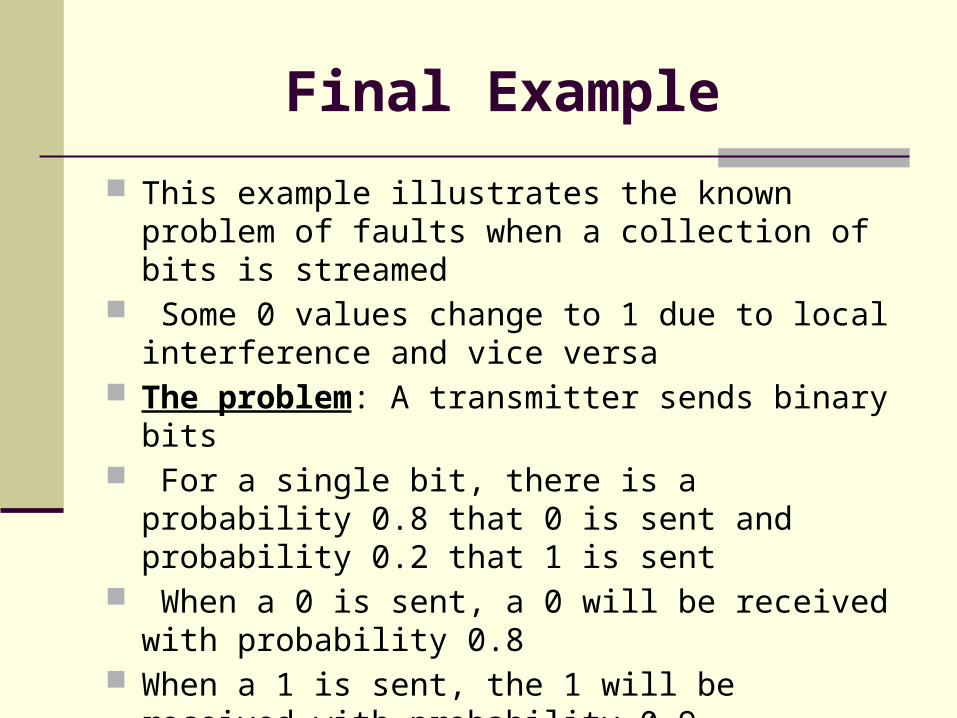
Final Example

This example illustrates the known problem of faults when a collection of bits is streamed

Some 0 values change to 1 due to local interference and vice versa

The problem: A transmitter sends binary bits For a single bit, there is a probability 0.8 that 0 is sent and

probability 0.2 that 1 is sent When a 0 is sent, a 0 will be received with probability 0.8 When a 1 is sent, the 1 will be received with probability

0.9

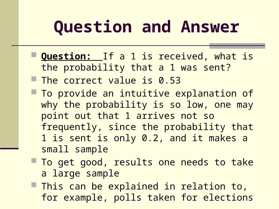
Question and Answer

Question: If a 1 is received, what is the probability that a 1 was sent?

The correct value is 0.53 To provide an intuitive explanation of why the probability

is so low, one may point out that 1 arrives not so frequently, since the probability that 1 is sent is only 0.2, and it makes a small sample

To get good, results one needs to take a large sample This can be explained in relation to, for example, polls

taken for elections

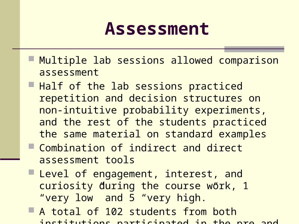
Assessment

Multiple lab sessions allowed comparison assessment Half of the lab sessions practiced repetition and decision

structures on non-intuitive probability experiments, and the rest of the students practiced the same material on standard examples

Combination of indirect and direct assessment tools Level of engagement, interest, and curiosity during the

course work, 1 “very low” and 5 “very high.” A total of 102 students from both institutions participated in

the pre and post survey

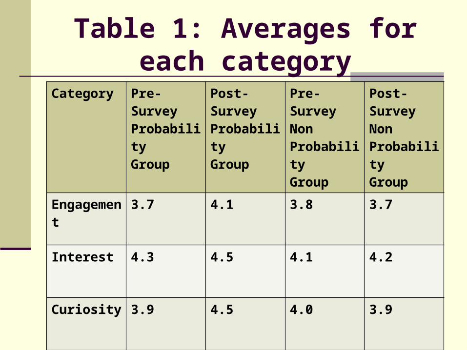
Table 1: Averages for each category

Category Pre-SurveyProbabilityGroup

Post-SurveyProbabilityGroup

Pre-SurveyNonProbabilityGroup

Post-SurveyNonProbabilityGroup

Engagement 3.7 4.1 3.8 3.7

Interest 4.3 4.5 4.1 4.2

Curiosity 3.9 4.5 4.0 3.9

Results

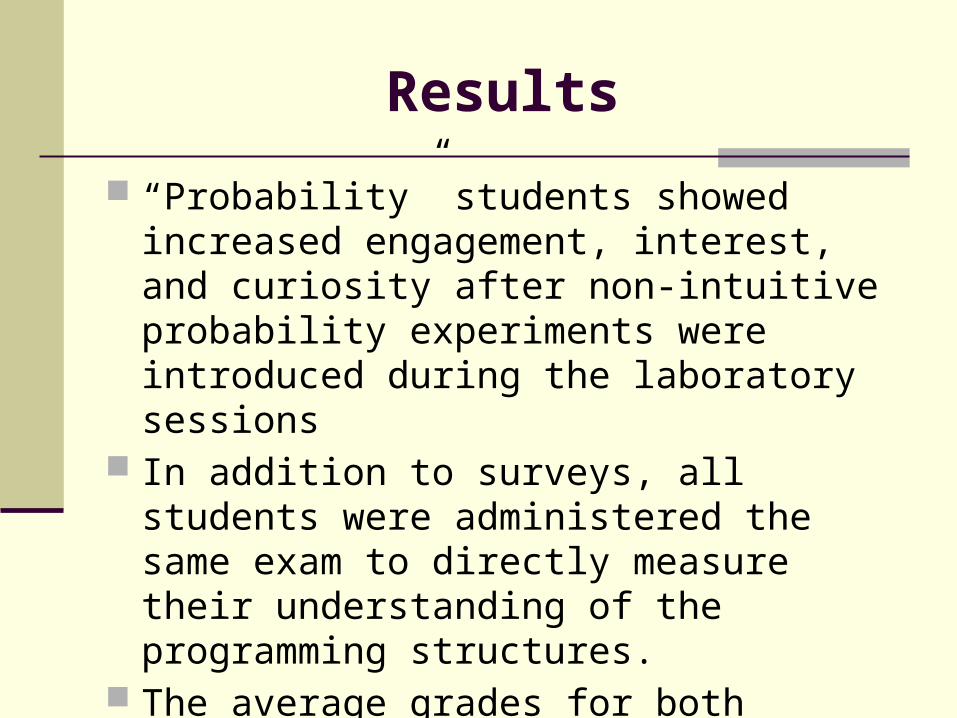
“Probability” students showed increased engagement, interest, and curiosity after non-intuitive probability experiments were introduced during the laboratory sessions

In addition to surveys, all students were administered the same exam to directly measure their understanding of the programming structures.

The average grades for both groups of students, before and after the probability component in the next table

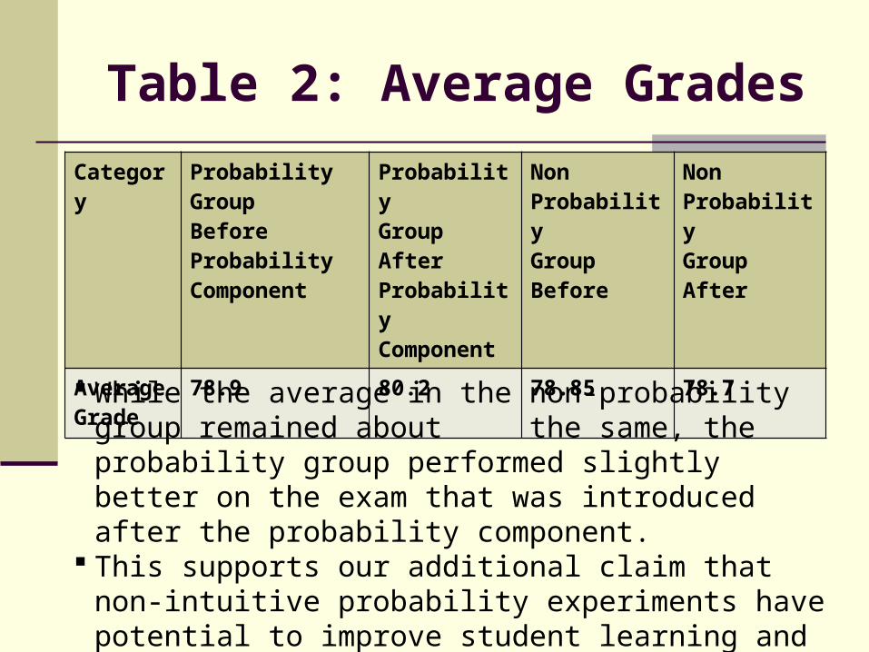
Table 2: Average Grades

Category ProbabilityGroupBeforeProbabilityComponent

ProbabilityGroupAfterProbabilityComponent

NonProbabilityGroupBefore

NonProbabilityGroupAfter

Average Grade

78.9 80.2 78.85 78.7

While the average in the non-probability group remained about the same, the probability group performed slightly better on the exam that was introduced after the probability component.

This supports our additional claim that non-intuitive probability experiments have potential to improve student learning and comprehension of the repetition and decision programming structures.

Summary and Future Plans

In general, the assessment results support our opinion on advantages of the proposed methodology

We are planning to continue inclusion of the probability experiments in the future iterations of the course

To integrate the proposed ideas into advanced courses, some of the examples could be generalized