Schroders The value of active management

December 2015

Schroder Investment Management Australia Limited Level 20, 123 Pitt Street, SYDNEY NSW 2000 Australian Financial Services Licence 226473 ABN 22 000 443 274

Schroders The value of active management by Greg Cooper, CEO, Schroder Investment Management Australia Ltd ________________________________________________________________

How much and for how long? Pension systems and their design have attracted considerable column inches over the years. From questions around the sustainability of corporate and government pension promises to the structure and costs of funding arrangements and the right investment approach, there has been no shortage of analysis and opinion. However, the biggest question that faces individuals (and taxpayers more broadly) is how much do I need to fund an adequate retirement? While the answer can and will always be “it depends”, the purpose of this paper is to consider some very long term scenarios and obtain some insights as to how much and on what it depends. Ultimately every dollar, pound, yen or euro that is deferred from current consumption (be it directly into a funded pension system or indirectly into a government tax pot from which pensions will be paid) will eventually yield some form of future consumption. However the size of that deferral, what happens to it during the deferral period, and then how much future consumption it needs to buy, gets to the heart of the pension funding problem. In particular, increases in longevity and changes in demographics have vastly altered the mathematics and the importance of the calculation. As governments and society gradually push more of the responsibility onto the individual for the provision of their future pension requirements, the potential to smooth over mistakes or “grow” our way out of it diminishes substantially. We would add that while investors may be currently cheering the actions of global central banks in providing “free money”, this is particularly bad news for those with some way to go to retirement or those requiring higher rates of return to fund retirement. In this paper we utilise over 300 years of historical UK equity and bond returns to analyse the impact of alternative contribution rate and pension payment policies. We are particularly focused on the impact at an individual level as with a defined contribution (DC) scheme but also maintaining broader macro-economic sustainability – what works for the individual must also work for the whole. By looking at what would have happened if we followed various funding and investment paths we aim to glean some insights into:

1. How much do I need to save; 2. How long will it last; 3. How should those savings be best invested; and 4. What else matters, and what doesn’t.

What does 300 years of history tell us? We have obtained UK equity, bond/interest rate and inflation data going back to 1694. This was around the period when John Castaing begins to issue “at this Office in Jonathan’s Coffee-house” a list of stock and commodity prices called “The Course of the Exchange and other things”. It is the earliest evidence of organised trading in marketable securities in London

1. Not long after Stockbrokers were banned from the Royal Exchange

for rowdiness (clearly some things never change). The period covers the industrial revolution, numerous regional and global wars, and the invention of almost everything that today underpins modern society. We have had the South Sea Bubble (think tech bubble), the invention and use of electricity, the telephone and modern transportation systems and a variety of geopolitical conflicts, all particularly disruptive events for corporates and broader industry at the time, and akin to today’s disruptions brought on by the internet and biotechnology.

1 Source: London Stock Exchange website

December 2015

2

Life expectancy then was only 35 or so years (because of high infant mortality, life expectancy after birth was somewhat higher) and so pension funding probably less of an issue as “retirement” wasn’t really a concept, or indeed one likely to last that long. However, by overlaying alternative accumulation and decumulation strategies on this period we can get some idea of what real world results would have been achieved and draw some inferences about how we might want to structure and invest pension schemes, particularly DC ones, going forward. While we might question the veracity of some of the older equity, bond and inflation data, the table below summarises the key outcomes over time and suggests that it is not out of line with more recent data and expectations.

UK Returns in GBP 1700’s 1800’s 1900’s 1694 to 2015

Nominal return on equities 6.0% 4.9% 8.8% 6.8% Nominal return on bonds 5.0% 4.0% 5.8% 4.9% Nominal return on 60/40* 5.7% 4.6% 7.9% 6.2%

Inflation 0.3% -0.1% 3.8% 1.4%

Real equities 5.7% 5.0% 5.0% 5.4% Real bonds 4.7% 4.1% 2.0% 3.5% Real 60/40* 5.4% 4.7% 4.1% 4.8%

*Denotes a portfolio that is 60% equities, 40% bonds. All return data in this paper is sourced from Global Financial Data. Bond returns have

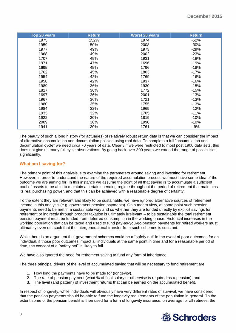
been proxied by using the Bank of England Base Rate (BOE) from 1695-1700, 60% Consols and 40% BOE from 1700-1932, and the UK 10 year government bond total return index for 1932-2015. Equity data is the UK-FTSE All Share Index. Inflation is the UK Retail Price Index. Given likely changes in data collection and reporting over the time frame we would be careful with looking beyond nominal and real returns in this dataset, however it is interesting to note that the volatility of the equity market return (standard deviation of annual results) was 11.9% in the 1700’s, only 6.9% in the 1800’s but surged to 21.6% since 1900. Given that the real return is essentially unchanged over these time frames, investors now get more risk for their return. We would also note that the data from a UK perspective suffers from a degree of positive selection bias – as it would for the US, Canada and Australia. We are looking back at a period of time that has been generally positive for the long term growth of these economies with relatively stable political and economic systems and no sovereign default. The same could not be said for say Argentinean, Chinese, German, Japanese or equity and bond investors, among others. Readers should bear this historical context in mind. We note that positive long term inflation has been a phenomenon of the 1900’s and beyond (with the advent of fiat money). However, irrespective of inflation the real return on equities has been remarkably consistent at circa 5% p.a, while bond holders have been the real sufferers from inflation with average real bond returns declining from 4-5% p.a. real in the 1700’s and 1800’s to 2% p.a. real in the post 1900’s (this may be partly due to the data veracity in bonds with that prior to 1932 being a proxy based on Consols and the Bank of England Base Rate). Interestingly the “extremes” of returns have been well dispersed through the 300 year history, with the possible exception of the outlier high inflation years of the mid 1970’s. The table below shows the 20 best and worst returns on UK equities and the corresponding year.

December 2015

3

Top 20 years Return Worst 20 years Return

1975 1959 1977 1968 1707 1971 1695 1762 1954 1958 1989 1817 1697 1967 1980 1984 1933 1922 2009 1941

152% 50% 49% 49% 49% 47% 45% 45% 42% 42% 36% 36% 36% 36% 35% 32% 32% 30% 30% 30%

1974 2008 1973 2002 1931 1696 1796 1803 1769 1937 1930 1772 2001 1721 1755 1969 1705 1819 1990 1761

-52% -30% -29% -23% -19% -19% -18% -17% -16% -16% -15% -15% -13% -13% -13% -12% -11% -10% -10% -9%

The beauty of such a long history (for actuaries) of relatively robust return data is that we can consider the impact of alternative accumulation and decumulation policies using real data. To complete a full “accumulation and decumulation cycle” we need circa 70 years of data. Clearly if we were restricted to most post 1900 data sets, this does not give us many full cycle observations. By going back over 300 years we extend the range of possibilities significantly.

What am I saving for?

The primary point of this analysis is to examine the parameters around saving and investing for retirement. However, in order to understand the nature of the required accumulation process we must have some idea of the outcome we are aiming for. In this instance we assume the point of all that saving is to accumulate a sufficient pool of assets to be able to maintain a certain spending regime throughout the period of retirement that maintains its real purchasing power, and that this can be achieved with a reasonable degree of certainty. To the extent they are relevant and likely to be sustainable, we have ignored alternative sources of retirement income in this analysis (e.g. government pension payments). On a macro view, at some point such pension payments need to be met in a sustainable way and so whether they are funded directly by explicit savings for retirement or indirectly through broader taxation is ultimately irrelevant – to be sustainable the total retirement pension payment must be funded from deferred consumption in the working phase. Historical increases in the working population that can be taxed and used to fund pay-as-you-go pension payments for retired workers must ultimately even out such that the intergenerational transfer from such schemes is constant. While there is an argument that government schemes could be a “safety net” in the event of poor outcomes for an individual, if those poor outcomes impact all individuals at the same point in time and for a reasonable period of time, the concept of a “safety net” is likely to fail. We have also ignored the need for retirement saving to fund any form of inheritance. The three principal drivers of the level of accumulated saving that will be necessary to fund retirement are:

1. How long the payments have to be made for (longevity). 2. The rate of pension payment (what % of final salary or otherwise is required as a pension); and 3. The level (and pattern) of investment returns that can be earned on the accumulated benefit.

In respect of longevity, while individuals will obviously have very different rates of survival, we have considered that the pension payments should be able to fund the longevity requirements of the population in general. To the extent some of the pension benefit is then used for a form of longevity insurance, on average for all retirees, the

December 2015

4

sums will be sufficient (particularly if such longevity insurance is provided by the government and free of “capital” charges and “profit” margin). This design issue is one we have explored in an Australian context but will revisit in a future paper

2.

Current longevity for a 65 year old male and 60 year old female is circa 18 years and 25 years respectively (UK 2006-2008 life tables, non-smokers). However, in 1900, the average life expectancy of a 65 year old male was around age 76 (so 11 years). This remained virtually unchanged until 1960 but since then longevity has increased at the rate of around 1 year every decade

3. Consequently, for someone starting out accumulating for

retirement today, with a planned retirement age of 65 in say 2055, the life expectancy is likely to be closer to 30 years using current rates of mortality improvement and allowing for higher life expectancies of working population over total population. While we have and are likely to see increasing rates of workforce participation from spouses, there is still also likely to be some requirement at least for retirement accumulation to cover joint lives rather than single lives (which results in a greater longevity requirement than for single lives). The table below provides an interesting perspective on the rate at which mortality improvement is taking place. While few would argue this is bad (maybe save a few children looking for their inheritance), it will clearly have an impact on the pension funding equation. Figure 1: Rising expectation of life at age 65 for England and Wales from 1850-2003

Source: Mortality improvements and evolution of life expectancies, Adrian Gallop, UK Government Actuaries Department, 2006

We have assumed for this paper that a drawdown period of 30 years is required. In respect of the rate of pension payment required we have used a measure based on final salary at the date of retirement. This allows us to automatically adjust for the likely lifestyle of the individual at that time and the fact that salary increases tend to be at a rate faster than inflation over time (broadly reflecting productivity improvements). However we also recognise that less than 100% of the final salary is required in retirement to reflect changing lifestyles and (usually) the lack of dependents and significant debt repayments. To this end we have used 65% of final salary as the “target” pension payment in retirement, but have also considered variations to this. We note that this is slightly less than the 70% recommended by the OECD

4

We also note that the pension requirement through retirement is unlikely to be constant, with lifestyle and living needs dominating the earlier years of retirement and health/aged care the latter years. For the sake of simplicity we have modelled a constant requirement of 65% of final salary, indexed with RPI (Retail Price Inflation), through

2 “Post Retirement – Time to Focus on the Endgame”, August 2011 and “Post Retirement Options for Funds”, January 2012,

Schroder Investment Management Australia Limited and “Global Lessons in Developing Post-Retirement Solutions”,

Schroders, May 2015 3 “Mortality improvements and evolution of life expectancies”, Adrian Gallop, UK Government Actuaries Department, 2006,

Page 3 4 “OECD Private Pensions Outlook 2008”, page 121

December 2015

5

the retirement years. The broader issue of fluctuating retirement needs is an aspect we intend to address in a later paper. We have assumed salary increases of 1% p.a. throughout the working career, however where salary inflation occurs at a higher or lower rate than 1% over RPI, a higher or lower level of contributions would be required, particularly if the pattern of wage inflation was not consistent through the working career. Earlier wage inflation would mean contributions could be lower, while higher wage inflation later in life would require much higher contribution rates. The chart below shows the real rate of wage inflation over the data period we are considering. Figure 2 – Rate of Change in Annual Real Earnings in the UK (20 year smoothed)

Source: Average earnings and retail prices, UK 1209-2010, Clark, University of California (2011) and www.measuringworth.com. Schroders chart based on 20 year annualised average rate of change.

Real wage increases in the UK have averaged 0.85% p.a. over the period since 1694, with an average rate of 0.25% p.a. in the 1700’s, 1.25% p.a. in the 1800’s and 1.23% p.a. since 1900. We also note the more recent decline in real wages of around 10% since 2007. In any case, a long term assumption of real wage increase of around 1% p.a. does not seem unrealistic.

Income – does it matter?

One solution that has been put forward to the pension funding problem is that the focus in product design should be around generating income. In particular, the high rates of dividend payments from all stocks, or a sub-section of stocks, can be a primary part of the solution. While this is a topic in and of itself

5 we can make a number of

observations that should dispel this notion as one that can be applied across the entire population:

1. If retirement income was to be generated solely from yield the accumulated retirement savings pot would have to be quite large to facilitate this and likely beyond the reasonable savings goals of most individuals. For example, a 4% constant yield would require an asset base of 25 times (1/0.04), so assuming a pension of 65% of salary this would require a starting pension pot of 16.25 times final salary (65% x 25). This is likely to be beyond the means or wishes for most individuals as it would represent considerable deferred consumption (and ultimately becomes an inheritance strategy not a retirement strategy).

5 For example “It’s not all about income”, Schroder Investment Management Australia Limited, May 2013

http://www.measuringworth.com/

December 2015

6

2. On the basis that retirement accumulation is typically tax advantaged, governments are unlikely to allow the significant drain on the tax pie that would result in large segments of the population “over-saving” for retirement. We already see a number of countries (including the UK and Australia) placing limits on the amount that can be accumulated at concessional tax rates in retirement vehicles.

3. At a macro level, if we all saved enough to fully fund retirement on yield alone, the savings pool within a generation or two would vastly exceed the ability of capital markets to support it (unless population growth was relatively large), and in the process drive down yields to where this was no longer sustainable.

4. Yield is just one part of the return equation and, through changes in dividend policy or financial structuring, can be (and is) manufactured. However, this does not alter total returns, it just shifts return from capital to income, and consequently total return is the only thing that matters. That said, if the amounts are large enough there is never a significant draw-down on the capital value and path dependency becomes less relevant, but again this is unlikely to be possible for most retirees and governments are unlikely to allow it.

5. If a subsection of high-yielding stocks (or bonds) was targeted for additional yield, equilibrium in capital markets would mean that the yield on these stocks gradually fell until it reached the market yield and, assuming these stocks were correctly priced for risk prior to the capital inflow, the result would now be that “high yield” investors were no longer being appropriately compensated for risk. This could well be the case now given the preponderance of high yield product and the actions of central banks to drive down overall yields, particularly on safer assets.

Consequently, we dispel the notion that retirement is about “income”. The decumulation process must be about total returns and the pattern of total returns (given that some level of capital drawdown must occur). Schroders has addressed this in other papers.

6 The only basis on which there should be some differential consideration in

income versus capital is to the extent there is some differential in the tax or other treatment of these components.

How much is enough?

Now we get to the nub of the problem. What level of savings is required to appropriately fund a reasonable level of drawdown in retirement? If we start by assuming a contribution rate of 8% (e.g. NEST, post 2018 minimum contribution rate), with no fees or charges deducted at any point (unrealistic obviously), salary inflation of circa 1% above retail price inflation, and 100% invested in UK equities, our accumulated balance after 40 years would have historically had a median result of 7.5 times salary. However, as shown in the chart below, there would have been considerable historical volatility around this result.

6 “Understanding the route to retirement” and “Understanding the Journey to Retirement” for UK and Australian perspectives

on the issue of path dependency, Schroders, May 2012. “Real World Post-Retirement Solutions”, Schroders Investment

Perspectives, December 2015

December 2015

7

Figure 4: Large volatility in value of a 40 Year accumulation at 8% of salary if 100% invested in UK equities with no fees or taxes.

0

5

10

15

20

25

16

95

17

03

17

11

17

19

17

27

17

35

17

43

17

51

17

59

17

67

17

75

17

83

17

91

17

99

18

07

18

15

18

23

18

31

18

39

18

47

18

55

18

63

18

71

18

79

18

87

18

95

19

03

19

11

19

19

19

27

19

35

19

43

19

51

19

59

19

67

Start year of accumulation. Salary increases at RPI+1%. Contribution Rate of 8% of Salary. 40 Year accumulation as a multiple of final salary. 100% equities/0% bonds.

We can observe that under this savings and investment scenario, the likely accumulated benefit has ranged from just over 2 times final salary to in excess of 22 times. Having accumulated this pot of saving, we can now estimate how long this would have lasted. In order to compare drawdown results (and the magnitude of the drawdown) we have chosen a fixed period with a constant real drawdown amount set initially as a percentage of final salary. We then analyse how much of the savings pot is left at the end of the drawdown period as a multiple of that starting final salary – this allows us to better compare numbers across different time periods. To the extent we run out of money in this drawdown process we have assumed the drawdowns carry on as a negative balance – this again gives us a sense of the magnitude of the shortfall over time rather than just saying we ran out of money after x years (bearing in mind that someone, e.g. the government, relatives, etc) would still have to fund some level of retirement income. The chart below shows the 30 year drawdown results with the starting balance accumulated from our 8% contributions above. Again for this exercise we have assumed 100% investment in UK equities (so the most aggressive, highest returning option available over time). The level of drawdown has been set at a very low 42% of final salary. This is the rate that on a median result uses up the entire starting balance, however as we can see the variability of the outcomes is enormous and highly cyclical.

December 2015

8

Figure 5: Significant volatility in the amount left after a 30 Year decumulation at 42% of final salary, assuming 100% invested in UK equities with no fees or taxes after a contribution rate of 8% of salary.

-12%

-8%

-4%

0%

4%

8%

12%

-25

-20

-15

-10

-5

0

5

10

15

20

25

17

35

17

42

17

49

17

56

17

63

17

70

17

77

17

84

17

91

17

98

18

05

18

12

18

19

18

26

18

33

18

40

18

47

18

54

18

61

18

68

18

75

18

82

18

89

18

96

19

03

19

10

19

17

19

24

19

31

19

38

19

45

19

52

19

59

19

66

19

73

Start year of decumulation. Decumulation rate assumed at 42% of final salary, indexed with RPI thereafter. Starting balance set at outcome of above 40 year accumulation. Decumulation

Process - 30 Year Results, 100% in UK equities/0% in UK bonds.

Amount left after 30 years (as a multiple of final salary)

Annualised real return for 30 years (rhs)

If we set our decumulation period as only 20 years, then the level of final salary supported as a pension rises to 52.5%, however the dispersion of results through time is still very large. The chart below provides a summary of some alternative outcomes if we assumed different (more conservative) investment portfolios.

30 year decumulation with 42% of final salary

As a multiple of final salary

Median amount at end 90th

percentile 10th

percentile

100% invested in UK equities

0.0 41.0 -22.5

60/40 portfolio -6.8 9.5 -30.5

100% invested in UK bonds

-11.5 4.3 -20.2

While the range of outcomes narrows slightly, the median result deteriorates markedly under more conservative investment portfolios. Put another way, if we assumed a typical balanced portfolio mix of 60% equities, 40% bonds, for the median outcome to be zero (the “perfect” drawdown rate where we run out of money at 30 years), then the level of final salary that can be supported as a pension falls to only 35%. Clearly an 8% accumulation is far too low to support realistic pension outcomes. If we reverse the question and consider what is a realistic contribution rate to support a 65% of final salary drawdown for 30 years, then assuming a 100% equity investment the required contribution rate (such that the median 30 year drawdown result of all time periods is zero) is circa 12.4% of salary with the range of outcomes shown below.

December 2015

9

Figure 6: Considerable volatility of outcomes after a 30 Year decumulation at 65% of final salary, 100% invested in UK equities, no fees or taxes. Contribution rate of 12.4% of salary.

-12%

-8%

-4%

0%

4%

8%

12%

-25

-20

-15

-10

-5

0

5

10

15

20

25

17

35

17

42

17

49

17

56

17

63

17

70

17

77

17

84

17

91

17

98

18

05

18

12

18

19

18

26

18

33

18

40

18

47

18

54

18

61

18

68

18

75

18

82

18

89

18

96

19

03

19

10

19

17

19

24

19

31

19

38

19

45

19

52

19

59

19

66

19

73

Start year of decumulation. Decumulation rate 65% of final salary. Starting balance outcome of 40 year accumulation and 12.4% contribution rate. Decumulation Process - 30 Year Results,

100% in UK equities/0% in UK bonds.



Clearly, while on average we are ok, the dispersion of outcomes remains very large (and for long periods of time). If we used a more balanced portfolio option of 60/40, the required contribution rate rises to about 14.8%, however the dispersion of outcomes remains very large (even at the 75 percentile and 25

th percentile the results are + or –

14 times final salary at the end of the decumulation process!). Note that the average real return of the 100% equities portfolio is 5.4% p.a. while the average real return of the balanced (60/40) portfolio is only 4.8% p.a. – what doesn’t sound like much of a difference has a very big impact. The chart below shows our 14.8% contribution rate decumulated for 30 years at 65% of final salary with a 60/40 balanced portfolio investment. Figure 7: 30 Year decumulation at 65% of final salary, 60% UK equities/40% bonds, no fees or taxes. Contribution rate of 14.8% of salary.

-12%

-8%

-4%

0%

4%

8%

12%

-25

-20

-15

-10

-5

0

5

10

15

20

25

17

35

17

42

17

49

17

56

17

63

17

70

17

77

17

84

17

91

17

98

18

05

18

12

18

19

18

26

18

33

18

40

18

47

18

54

18

61

18

68

18

75

18

82

18

89

18

96

19

03

19

10

19

17

19

24

19

31

19

38

19

45

19

52

19

59

19

66

19

73


60% in UK equities/40% in UK bonds.



December 2015

10

What’s the real problem?

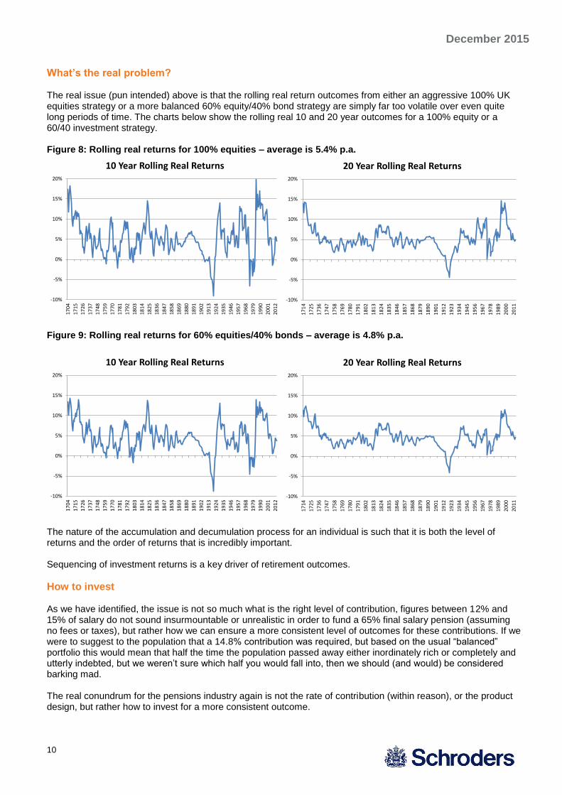
The real issue (pun intended) above is that the rolling real return outcomes from either an aggressive 100% UK equities strategy or a more balanced 60% equity/40% bond strategy are simply far too volatile over even quite long periods of time. The charts below show the rolling real 10 and 20 year outcomes for a 100% equity or a 60/40 investment strategy. Figure 8: Rolling real returns for 100% equities – average is 5.4% p.a.

-10%

-5%

0%

5%

10%

15%

20%

17

04

17

15

17

26

17

37

17

48

17

59

17

70

17

81

17

92

18

03

18

14

18

25

18

36

18

47

18

58

18

69

18

80

18

91

19

02

19

13

19

24

19

35

19

46

19

57

19

68

19

79

19

90

20

01

20

12

10 Year Rolling Real Returns

-10%

-5%

0%

5%

10%

15%

20%

17

14

17

25

17

36

17

47

17

58

17

69

17

80

17

91

18

02

18

13

18

24

18

35

18

46

18

57

18

68

18

79

18

90

19

01

19

12

19

23

19

34

19

45

19

56

19

67

19

78

19

89

20

00

20

11


Figure 9: Rolling real returns for 60% equities/40% bonds – average is 4.8% p.a.

-10%

-5%

0%

5%

10%

15%

20%

17

04

17

15

17

26

17

37

17

48

17

59

17

70

17

81

17

92

18

03

18

14

18

25

18

36

18

47

18

58

18

69

18

80

18

91

19

02

19

13

19

24

19

35

19

46

19

57

19

68

19

79

19

90

20

01

20

12


-10%

-5%

0%

5%

10%

15%

20%

17

14

17

25

17

36

17

47

17

58

17

69

17

80

17

91

18

02

18

13

18

24

18

35

18

46

18

57

18

68

18

79

18

90

19

01

19

12

19

23

19

34

19

45

19

56

19

67

19

78

19

89

20

00

20

11


The nature of the accumulation and decumulation process for an individual is such that it is both the level of returns and the order of returns that is incredibly important. Sequencing of investment returns is a key driver of retirement outcomes.

How to invest As we have identified, the issue is not so much what is the right level of contribution, figures between 12% and 15% of salary do not sound insurmountable or unrealistic in order to fund a 65% final salary pension (assuming no fees or taxes), but rather how we can ensure a more consistent level of outcomes for these contributions. If we were to suggest to the population that a 14.8% contribution was required, but based on the usual “balanced” portfolio this would mean that half the time the population passed away either inordinately rich or completely and utterly indebted, but we weren’t sure which half you would fall into, then we should (and would) be considered barking mad. The real conundrum for the pensions industry again is not the rate of contribution (within reason), or the product design, but rather how to invest for a more consistent outcome.

December 2015

11

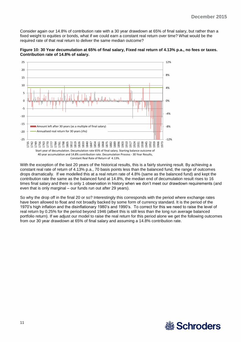
Consider again our 14.8% of contribution rate with a 30 year drawdown at 65% of final salary, but rather than a fixed weight to equities or bonds, what if we could earn a constant real return over time? What would be the required rate of that real return to deliver the same median outcome? Figure 10: 30 Year decumulation at 65% of final salary, Fixed real return of 4.13% p.a., no fees or taxes. Contribution rate of 14.8% of salary.

-12%

-8%

-4%

0%

4%

8%

12%

-25

-20

-15

-10

-5

0

5

10

15

20

25

17

35

17

42

17

49

17

56

17

63

17

70

17

77

17

84

17

91

17

98

18

05

18

12

18

19

18

26

18

33

18

40

18

47

18

54

18

61

18

68

18

75

18

82

18

89

18

96

19

03

19

10

19

17

19

24

19

31

19

38

19

45

19

52

19

59

19

66

19

73


Constant Real Rate of Return of 4.13%.



With the exception of the last 20 years of the historical results, this is a fairly stunning result. By achieving a constant real rate of return of 4.13% p.a., 70 basis points less than the balanced fund, the range of outcomes drops dramatically. If we modelled this at a real return rate of 4.8% (same as the balanced fund) and kept the contribution rate the same as the balanced fund at 14.8%, the median end of decumulation result rises to 16 times final salary and there is only 1 observation in history when we don’t meet our drawdown requirements (and even that is only marginal – our funds run out after 29 years). So why the drop off in the final 20 or so? Interestingly this corresponds with the period where exchange rates have been allowed to float and not broadly backed by some form of currency standard. It is the period of the 1970’s high inflation and the disinflationary 1980’s and 1990’s. To correct for this we need to raise the level of real return by 0.25% for the period beyond 1946 (albeit this is still less than the long run average balanced portfolio return). If we adjust our model to raise the real return for this period alone we get the following outcomes from our 30 year drawdown at 65% of final salary and assuming a 14.8% contribution rate.

December 2015

12

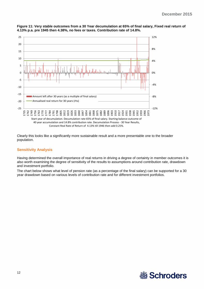
Figure 11: Very stable outcomes from a 30 Year decumulation at 65% of final salary, Fixed real return of 4.13% p.a. pre 1945 then 4.38%, no fees or taxes. Contribution rate of 14.8%.

-12%

-8%

-4%

0%

4%

8%

12%

-25

-20

-15

-10

-5

0

5

10

15

20

25

17

35

17

42

17

49

17

56

17

63

17

70

17

77

17

84

17

91

17

98

18

05

18

12

18

19

18

26

18

33

18

40

18

47

18

54

18

61

18

68

18

75

18

82

18

89

18

96

19

03

19

10

19

17

19

24

19

31

19

38

19

45

19

52

19

59

19

66

19

73


Constant Real Rate of Return of 4.13% till 1946 then add 0.25%.



Clearly this looks like a significantly more sustainable result and a more presentable one to the broader population.

Sensitivity Analysis

Having determined the overall importance of real returns in driving a degree of certainty in member outcomes it is also worth examining the degree of sensitivity of the results to assumptions around contribution rate, drawdown and investment portfolio.

The chart below shows what level of pension rate (as a percentage of the final salary) can be supported for a 30 year drawdown based on various levels of contribution rate and for different investment portfolios.

December 2015

13

Figure 12: Level of final salary pension supported at various contribution rates and under alternative investment scenarios

0

10

20

30

40

50

60

70

80

90

100

60/40 100% equities 100% bonds 4.65% Real 5% Real 4% Real 3% Real

Pe

nsi

on

Rat

e S

up

po

rte

d %

Fin

al S

alar

y

Investment Portfolio

10% 12%

14% 16%

We can see from the above that:

a) For each 2% rise in the contribution rate, the level of final salary pension rises by approximately 9% under a 60/40 portfolio, 11% in a 100% equity portfolio and 6% for a pure bond portfolio, and more generally by around 2% for every 1% of real return that we earn.

b) The median results from a 4.65% p.a. real return portfolio are the same as the median results from a 100% equity portfolio, even though the average return on the equity portfolio is 5.4% p.a. This highlights the importance of sequencing risk in outcomes. A balanced fund had a substantially worse median result than the 4.65% real portfolio, yet the average return on a balanced fund was 4.8%.

c) If we suggested that a long term level of sustainability was around 60% of final salary, we either need

contribution rates of 14%+ or a 12% contribution rate in combination with a real return strategy. Of course the other relevant aspect of our sensitivity analysis is the degree of variability in the results from different contribution rate and investment strategies. The chart below shows for a given final pension the range of outcomes (defined as the value of our retirement pool after a 30 year drawdown as a multiple of our final salary at retirement) from a 14% contribution rate under various investment strategies (the final pension result is the same as that from figure 12 above at the 14% contribution rate that at the median level is “perfect”).

December 2015

14

Figure 13: Range of drawdown outcomes from different contribution rate and investment strategies

-20

-15

-10

-5

0

5

10

15

20

25

0%

10%

20%

30%

40%

50%

60%

70%

80%

90%

60/40 100% equity 100% bonds Real 4.65% Variable4.65%

Real 5% Real 4% Real 3%

Mu

ltip

le o

f Fi

nal

Sal

ary

at E

nd

of

Dra

wd

ow

n

Pe

rce

nta

ge o

f Fi

nal

Sal

ary

Sup

po

rte

d

Investment Strategy

Pension supported (lhs)

Median (rhs)

We can observe from the above that under various fixed asset allocation scenarios, even 100% bonds, the range of results is significantly greater than that under the real return scenarios. This is even the case when we allow for a variable real return (+/- 5% from year to year as per Figure 14 below).

The obvious conclusion from this is that the biggest driver of sustainability of pension outcomes is in fact stability of the real return outcome. It is not the amount in equities or bonds, nor (within bounds) the contribution rate. It is stable, real returns. What this means is that the inordinate focus of the industry on investment structures, product design, active vs passive etc etc, matters for little. Having the flexibility to adjust the investment policy to explicitly target real returns (which by definition requires an active approach to management) is the most important piece of the puzzle.

What’s it worth? Two important questions we can consider now are:

1. Just how stable do real returns need to be (clearly stability on a rolling 12 month basis would be nice but probably unrealistic, while stability on a 3 to 5 year view is far more achievable); and

2. What is this worth? To address the first point we have remodelled our results from figure 11 above but where the real return is stable on a 10 year time horizon only, within that 10 years the fluctuations vary by up to +/- 5%. The outcomes are shown in the chart below.

December 2015

15

Figure 14: Significantly lower volatility in outcomes from a 30 Year decumulation at 65% of final salary, Fixed real return of 4.13% p.a. pre 1945 then 4.38% but with yearly variability of +/-5%, no fees or taxes. Contribution rate of 14.8%.

-12%

-8%

-4%

0%

4%

8%

12%

-25

-20

-15

-10

-5

0

5

10

15

20

25

17

35

17

42

17

49

17

56

17

63

17

70

17

77

17

84

17

91

17

98

18

05

18

12

18

19

18

26

18

33

18

40

18

47

18

54

18

61

18

68

18

75

18

82

18

89

18

96

19

03

19

10

19

17

19

24

19

31

19

38

19

45

19

52

19

59

19

66

19

73


Constant Real Rate of Return of 4.13% till 1946 then add 0.25%.



While the results are more volatile, the overall volatility of outcomes is still substantially less than that of our alternative more traditional portfolios. The range of outcomes form the 75

th percentile to the 25

th percentile is 1.9

times final salary to -3.5 times final salary. Consequently, targeting real returns on a medium term basis gives a substantially more predictable and lower overall cost outcome than current portfolio construction methodologies. While the investment side of the pensions industry has largely focussed on fixed strategic asset allocations as the building blocks of the investment strategy, it is clear from the results in this paper that we should be providing much great emphasis on the provision of stable real returns. While stable real returns are not at all easy to achieve there is considerable value to retirees in being able to do this. We have shown in this paper that the long term return could be nearly 80 basis points lower than equivalent equity return (equity return of 5.4% real vs a fixed real return of 4.65%) while delivering the same outcome and considerably lower volatility of the outcomes. Similarly, the long term returns could be 40 to 50 basis points lower than that of a balanced fund and still deliver the same outcome with a considerably greater certainty (4.13% to 4.38% fixed real vs a balanced fund of 4.8%). Recognising that returns could be lower while the average benefit remains the same, and the certainty of delivery of outcomes is considerable improved, investors should absolutely be prepared to pay for this stability. Put another way, if we set the constant real return at the same as a balanced fund (which is not free to implement of course), then we could support a pension payment of 82% of salary rather than 65%, with significantly more certainty. I have little doubt the population as a whole would regard this as “value for money”. In a nutshell, the value of adopting an outcome orientated approach and reducing overall volatility is considerable – 40 to 50 basis points in return terms alone, but massive in terms of the additional certainty it provides the broader population on retirement outcomes. While building portfolios that meet these more stable return requirements is not easy, it represents potentially very large value add.

7

Conclusion

By utilising a very long set of historical data we have shown that:

7 For an initial view on this see “Anchoring strategic asset allocation to valuation rather than to averages”, Schroder

Investment Management Australia Limited, February 2015 and “Outcome-oriented investing: Translating real world targets

into achievable investment objectives, Schroders, March 2015”

December 2015

16

1. A contribution rate of circa 12-15% over a 40 year career is a more realistic rate across the population in order to fund a 65% of final salary pension for a 30 year duration, where 30 years has been chosen as the likely longevity of a future 60/65 year old couple. We note that in the real world a higher contribution rate would be required to account for any fees and taxes.

2. Under normal portfolio constructs in the industry today, the range of outcomes that such a funding and drawdown policy achieves is too wide to be practically useful for individuals. Such policies may work where there is a sponsor (government or corporate) with the resources and patience to operate intergenerational smoothing, but I doubt that government or corporate really exists.

3. An emphasis on “income” as the driver of the investment portfolio is spurious, what matters is the ability to achieve more constant real outcomes through time (and not necessarily year on year, but certainly over 5 to 10 year periods). Typical portfolio constructs simply do not achieve this.

4. By being able to build portfolios that achieve more stable real return outcomes, the costs to society of pension funding become substantially more predictable and actually fall.

5. The value to society of an active approach to managing the retirement savings pool in line with real return outcomes is “worth” at least 40-50 basis points of incremental return, but substantially more in terms of the reduction in volatility (or rather the increase in certainty) it provides.

While the industry broadly has spent considerable time and energy, and continues to spend such time and energy, debating the merits of active vs passive management or reducing fees through amalgamation, this is entirely the wrong debate. By orders of magnitude the focus should be on building portfolios (which by their nature would have to be flexible and actively managed – at least at the asset allocation level) to achieve more constant real return outcomes. This is absolutely what the asset management industry should be empowered with providing and, as we have shown, is a very valuable service to the community as a whole - or put another way, worth paying for.

Disclaimer Opinions, estimates and projections in this report constitute the current judgement of the author as of the date of this article. They do not necessarily reflect the opinions of Schroder Investment Management Australia Limited, ABN 22 000 443 274, AFS Licence 226473 ("SIMAL") or any member of the Schroders Group and are subject to change without notice. In preparing this document, we have relied upon and assumed, without independent verification, the accuracy and completeness of all information available from public sources or which was otherwise reviewed by us.

SIMAL does not give any warranty as to the accuracy, reliability or completeness of information which is contained in this article. Except insofar as liability under any statute cannot be excluded, Schroders and its directors, employees, consultants or any company in the Schroders Group do not accept any liability (whether arising in contract, in tort or negligence or otherwise) or any error or omission in this article or for any resulting loss or damage (whether direct, indirect, consequential or otherwise) suffered by the recipient of this article or any other person.

This document does not contain, and should not be relied on as containing any investment, accounting, legal or tax advice. Past performance is not a reliable indicator of future performance. Unless otherwise stated the source for all graphs and tables contained in this document is SIMAL. For security purposes telephone calls may be taped.

Documents

Schroders The value of active management