Embed Size (px)
Citation preview

Schoo l o f Sc ience
Conceptual organization and retrieval in semantic memory: the differential role of switching and
clustering, acquisition and impairment in neurodegenerative conditions.
Joaquín Goñi Cortés

Servicio de Publicaciones de la Universidad de Navarra
ISBN 978-84-8081-368-6


F a c u l t a d d e C i e n c i a s
Conceptual organization and retrieval in semantic
memory: the differential role of switching and clustering, acquisition and impairment in
neurodegenerative conditions.
Submitted by Joaquín Goñi Cortés in partial fulfillment of the requirements for the Doctoral Degree of the University of Navarra
This dissertation has been written under our supervision at the Department of Physics and Applied Mathematics, and we approve its submission to the Defense Committee.
Signed on December 01, 2008
Sergio Ardanza-Trevijano Moras, PhD. Pablo Villoslada Díaz, PhD.


Declaración:
Por la presente yo, D. Joaquín Goñi Cortés, declaro que esta tesis es fruto de mi propiotrabajo y que en mi conocimiento, no contiene ni material previamente publicado o escrito porotra persona, ni material que sustancialmente haya formado parte de los requerimientos paraobtener cualquier otro título en cualquier centro de educación superior, excepto en los lugaresdel texto en los que se ha hecho referencia explícita a la fuente de la información.
(I hereby declare that this submission is my own work and that, to the best of my knowledge andbelief, it contains no material previously published or written by another person nor materialwhich to a substantial extent has been accepted for the award of any other degree of theuniversity or other institute of higher learning, except where due acknowledgment has beenmade in the text.)
De igual manera, autorizo al Departamento de Física y Matemática Aplicada de la Universidadde Navarra, la distribución de esta tesis y, si procede, de la “fe de erratas” correspondiente porcualquier medio, sin perjuicio de los derechos de propiedad intelectual que me corresponden.
Signed on December 18, 2008
Joaquín Goñi Cortés
c© Joaquín Goñi Cortés
Derechos de edición, divulgación y publicación:c© Departamento de Física y Matemática Aplicada, Universidad de Navarra


A mi familia,

Acknowledgements
Agradezco a todos mis companeros del departamento de Fısica y Matematica Aplicada de la
Universidad de Navarra y del departamento de Neurociencias del Centro de Investigacion Medica
Aplicada. En particular, son muchas las personas a las que deberıa mencionar y que de una
manera u otra me han ayudado. me han ensenado, o simplemente he tenido el placer de aprender
a su lado y por tanto tienen que ver directa o indirectamente con el trabajo desarrollado todos es-
tos anos. Especiales agredecimientos a: Arcadi Navarro, Agustın Garcıa Peiro, Pablo Villoslada,
Sergio Ardanza, Ricardo Palacios, Antonio Pelaez, Jorge Sepulcre, Nieves Velez de Mendizabal,
Jean Bragard, Francisco J. Esteban, Bartolome Bejarano, Jorge Elorza, Dennis P. Wall, Leonid
Peshkin, Angel Garcimartın, Inigo Martincorena, Gonzalo Arrondo, Hector Mancini, John Wes-
seling, Francisco Javier Novo, Herminia Peraita, Ricard V. Sole, Carlos Rodrıguez Caso, Andreea
Munteanu, Bernat Corominas y Lluis Samaranch.

Ante todo debemos preservar la absoluta imprevisibilidad y la total improbabilidad de
nuestras mentes interconectadas. De ese modo podremos mantener abiertas todas las
posibilidades, como hemos hecho en el pasado.
Serıa bueno contar con mejores metodos de monitorizar los cambios para poder reconocerlos
mientras estan ocurriendo... Tal vez las computadoras puedan hacerlo posible, aunque lo
dudo bastante. Se pueden crear modelos simulados de ciudades, pero lo que se deduce de
ellos es que parecen estar mas alla del alcance del analisis inteligente... Esto es interesante,
dado que una ciudad es la mayor concentracion posible de seres humanos y todos ejercen
tanta influencia como la que son capaces de soportar. La ciudad parece tener vida propia.
Si no podemos entender como funciona, no llegaremos muy lejos en la comprension general
de la sociedad humana.
Y sin embargo, deberıa ser posible. Reunida, la gran masa de mentes humanas de todo
el mundo parece comportarse como un sistema vivo coherente. El problema es que el
flujo de informacion es casi siempre unidireccional. A todos nos obsesiona la necesidad
de proporcionar informacion tan rapido como podamos, pero carecemos de mecanismos
eficaces para extraer algo a cambio. Confieso no saber mas de lo que ocurre en la mente
humana que lo que se de la mente de una hormiga. Ahora que lo pienso, ese podrıa ser un
buen punto de partida.
Lewis Thomas, 1973

CONTENTS XI
Contents
Preface XIII
1. Introduction 1
1.1. The human brain . . . . . . . . . . . . . . . . . . . . . . . . . . . . . . . . . . . . . 2
1.2. Memory and its different classifications . . . . . . . . . . . . . . . . . . . . . . . . . 7
1.3. Verbal fluency tasks . . . . . . . . . . . . . . . . . . . . . . . . . . . . . . . . . . . 12
1.4. Network theory and exploration phenomena . . . . . . . . . . . . . . . . . . . . . . 13
2. Frequency patterns and heterogeneity of concepts in verbal fluency 17
2.1. The experimental dataset of verbal fluency . . . . . . . . . . . . . . . . . . . . . . 18
2.2. Frequency distribution of words . . . . . . . . . . . . . . . . . . . . . . . . . . . . . 19
2.3. Word position and word heterogeneity rate . . . . . . . . . . . . . . . . . . . . . . 24
3. Conceptual network topology and switching-clustering differential retrieval 27
3.1. Towards an unsupervised model of conceptual organization . . . . . . . . . . . . . 28
3.2. Unsupervised generation of a conceptual network . . . . . . . . . . . . . . . . . . . 30
3.3. Modularity of the conceptual network . . . . . . . . . . . . . . . . . . . . . . . . . 34
3.4. Conceptual network enrichment and topological evaluation . . . . . . . . . . . . . 40
3.5. Accessibility and diffusivity patterns . . . . . . . . . . . . . . . . . . . . . . . . . . 45
3.6. Discussion . . . . . . . . . . . . . . . . . . . . . . . . . . . . . . . . . . . . . . . . . 48
4. Switcher random walks: a cognitive inspired strategy for network exploration 51
4.1. Introduction . . . . . . . . . . . . . . . . . . . . . . . . . . . . . . . . . . . . . . . . 52
4.2. A Markov model of SRW . . . . . . . . . . . . . . . . . . . . . . . . . . . . . . . . 55
4.2.1. Markov Chains . . . . . . . . . . . . . . . . . . . . . . . . . . . . . . . . . . 55
4.2.2. Graph Characterization . . . . . . . . . . . . . . . . . . . . . . . . . . . . . 55
4.2.3. Random walk over a graph as a Markov Process . . . . . . . . . . . . . . . 59
4.2.4. Switcher-random-walks . . . . . . . . . . . . . . . . . . . . . . . . . . . . . 59
4.3. Results & discussion . . . . . . . . . . . . . . . . . . . . . . . . . . . . . . . . . . . 63
5. Switcher Random Walks on the conceptual network ECN 65
5.1. Cognitive background and motivation . . . . . . . . . . . . . . . . . . . . . . . . . 66
5.2. Two variants of switcher random walkers . . . . . . . . . . . . . . . . . . . . . . . 67
5.3. Performance study of SRW exploration over ECN . . . . . . . . . . . . . . . . . . . 69
6. An ontogenic model of the conceptual network ECN 73
6.1. Introduction . . . . . . . . . . . . . . . . . . . . . . . . . . . . . . . . . . . . . . . . 74
6.2. Frequency in verbal fluency: an estimator of ranked age of acquisition . . . . . . . 75

XII CONTENTS
6.3. Topological measurements . . . . . . . . . . . . . . . . . . . . . . . . . . . . . . . . 76
6.4. Results and discussion . . . . . . . . . . . . . . . . . . . . . . . . . . . . . . . . . . 78
7. Lexical access impairment in neurodegenerative conditions 83
7.1. Multiple sclerosis . . . . . . . . . . . . . . . . . . . . . . . . . . . . . . . . . . . . . 84
7.2. Mild cognitive impairment . . . . . . . . . . . . . . . . . . . . . . . . . . . . . . . . 86
7.3. Alzheimer’s disease . . . . . . . . . . . . . . . . . . . . . . . . . . . . . . . . . . . . 87
7.4. Lexical access impairment . . . . . . . . . . . . . . . . . . . . . . . . . . . . . . . . 89
7.5. Verbal fluency datasets and their comparisons . . . . . . . . . . . . . . . . . . . . . 90
7.6. Results and discussion . . . . . . . . . . . . . . . . . . . . . . . . . . . . . . . . . . 93
8. Conclusions and Outlook 97
8.1. Conclusions . . . . . . . . . . . . . . . . . . . . . . . . . . . . . . . . . . . . . . . . 97
8.2. Outlook . . . . . . . . . . . . . . . . . . . . . . . . . . . . . . . . . . . . . . . . . . 98
A. Words and their frequency in the 200 verbal fluency tests 101
B. Modules identified in the conceptual network CN 113
C. Age of acquisition of animals and their frequency in verbal fluency 123

XIII
Preface
Semantic memory organization and retrieval is a cutting edge topic that is being studied from
different fields such as Linguistics, Psychology, Computer Science and Neuroscience. The aim of
this thesis is to improve the understanding of conceptual organization and retrieval by means of
network theory and the use of semantic verbal fluency tests (animals) in an unsupervised fashion.
Conceptual organization will be studied here as a complex network attached to a dual-mechanism
of information retrieval, i.e. switching and clustering.
The chapters are organized as follows: 1. An introduction to the concepts of human brain,
memory and network theory. 2. A study of the frequency patterns obtained from the verbal flu-
ency tests. 3. Development of a statistical method for the unsupervised generation of a conceptual
network and the in-silico evaluation of switching and clustering. Such evaluation together with
the definition of accessibility and diffusivity measurements allowed the decoupling of switching
and clustering functioning. 4. Study of switcher random walks (by means of finite Markov chains)
as an exploration-propagation paradigm in a number of in-silico network models. 5. Modeliza-
tion of the switching-clustering retrieval on the conceptual network obtained in chapter 3. 6. A
model of concept acquisition and semantic growth based on frequency of concepts. 7. Study of
the lexical access impairment in three different neurodegenerative conditions: Multiple Sclerosis,
Mild Cognitive Impairment and Alzheimer’s disease. 8. General conclusions and outlook of this
work

XIV Preface

1
Chapter 1
Introduction
An introduction to human brain, memory and network theory.
2 Introduction
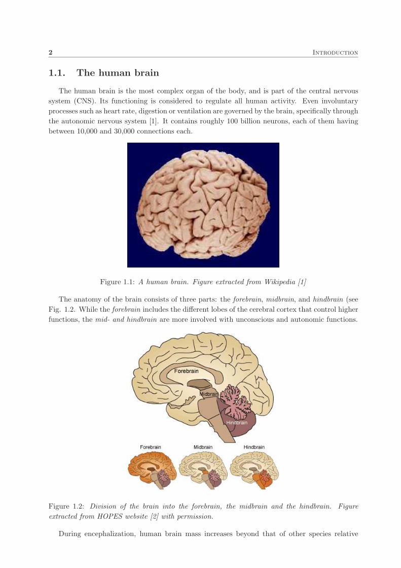
1.1. The human brain
The human brain is the most complex organ of the body, and is part of the central nervous
system (CNS). Its functioning is considered to regulate all human activity. Even involuntary
processes such as heart rate, digestion or ventilation are governed by the brain, specifically through
the autonomic nervous system [1]. It contains roughly 100 billion neurons, each of them having
between 10,000 and 30,000 connections each.
Figure 1.1: A human brain. Figure extracted from Wikipedia [1]
The anatomy of the brain consists of three parts: the forebrain, midbrain, and hindbrain (see
Fig. 1.2. While the forebrain includes the different lobes of the cerebral cortex that control higher
functions, the mid- and hindbrain are more involved with unconscious and autonomic functions.
Figure 1.2: Division of the brain into the forebrain, the midbrain and the hindbrain. Figure
extracted from HOPES website [2] with permission.
During encephalization, human brain mass increases beyond that of other species relative

Section 1.1 3
to body mass. This process is very pronounced in the neocortex, which is a part involved in
language and consciousness. The neocortex accounts for about 76% of the the human brain
mass. This percentage is much larger than in other animals and allows humans to enjoy unique
mental capacities despite having a neuroarchitecture similar to more primitive species. Indeed,
human consciousness is founded upon the extended capacity of the modern neocortex, as well
as the greatly developed structures of the brain stem. On the other hand, basic systems that
alert humans to stimuli, sense events in the environment, and maintain homeostasis are similar
to those of basic vertebrates.
The aspects of human brain regarding its partition in different lobes, its neurophysiology and
its implication in language are described below (see [1, 3] for detailed reviews).
Lobes of the brain
Although the lobes of the brain were originally a purely anatomical classification, they have
become also related to different brain functions. The telencephalon, the largest portion of the
human brain, is divided into 4 lobes (see [3] for a detailed review) Frontal lobe, that includes
conscious thought and can result in mood changes when is damaged, is crucial for future action
planning and control of movements. Parietal lobe is involved in integrating sensory information
from a number of senses, and with the manipulation of objects. Additionally, portions of the
parietal lobe are also related to visuospatial processing. Occipital lobe includes the sense of sight
and its damage can produce hallucinations. Temporal lobe includes senses of smell and sound, an
the processing of complex stimuli such as faces and scenes. The location of each lobe within the
brain can be seen in figure 1.3
Figure 1.3: Location of the 4 lobes of the brain: frontal (in blue), parietal (in yellow), occipital
(in pink) and temporal (in green). Cerebellum area is colored in white.
Neurophysiology
The human brain is the source of the conscious, cognitive mind [1]. The mind can be defined
as the set of cognitive processes involved in perception, imagination, interpretation, memories,
and language of which individuals may or may not be aware. Apart from cognitive functions,

4 Introduction
the brain also regulates autonomic processes related to vital body functions such as ventilation,
blood pressure and heart beating.
As commented at the beginning of this section, the extended neocortical capacity allows hu-
mans certain control over emotional behavior. Emotional pathways are able to modulate spon-
taneous emotive expression disregarding attempts at cerebral self-control. An emotive stability
of the mind has been associated with planning, experience, and an a stable and stimulating
environment.
The finding in the 19th century of the primary motor cortex mapped to correspond with
regions of the body led to popular belief that the brain was organized around a homunculus
(metaphorically, little man in charge of the functioning of a system; see Fig. 1.4).
Figure 1.4: Metaphor of the homunculus. Figure extracted from Wikipedia [4].
A distorted figure drawn to represent the body’s motor map in the prefrontal cortex is known
as the brain’s homunculus. Nevertheless human brain functioning is much more complex than this
simple figure suggests. Indeed, a similar, sensory homunculus can be drawn in the parietal lobe
that parallels that in the frontal lobe. Both representations of sensory and motor homunculus
can be seen at Fig. 1.5.
However, the human brain appears to have no localized center of conscious control. It is more
likely to derive consciousness from interactions among a large number of systems within the brain.
Executive functions rely on cerebral activities, especially those of the frontal lobes, but redundant
and complementary processes within the brain result in a diffuse assignment of executive control
that is certainly difficult to attribute to any single localization. For instance, visual perception is
generally processed in the occipital lobe, whereas the primary auditory cortex is located in the
temporal lobe.
Although a complete description of the biological basis for consciousness so far eludes the
scientific knowledge, reasonable assumptions have been provided. They have been possible due
to observable behaviors and on related internal responses that have provided the basis for general
classification of elements of consciousness and the neural regions associated with those elements.
For example, nowadays we know that people lose consciousness and regain it, partial losses of
consciousness associated with particular neuropathologies have been identified and the presence
of specific neural structures have happened to be necessary for certain conscious activities [1].

Section 1.1 5
Figure 1.5: Sensory (left) and motor (right) homunculus, i.e., distorted human figure drawn to
reflect the relative space our body parts occupy on the somatosensory cortex and the motor cortex
respectively. Figure including both maps was drawn by Dr. Penfield in 1951 and has been extracted
from Wikimedia [5].
Neurolinguistics
The specialized language areas are usually considered to be in the left hemisphere. Neverthe-
less, while this holds true for 97% of right-handed people, about 19% of left-handed people have
their language areas in the right hemisphere and a 68% of them have some language abilities in
both left and right hemispheres. Indeed, the two hemispheres are thought to contribute to the
processing and understanding of language: the left hemisphere processes the linguistic meaning
of prosody, while the right hemisphere processes the emotions conveyed by prosody. Studies on
children have provided some interesting findings: a child with damage to the left hemisphere, may
develop language in the right hemisphere instead. In particular, the younger the child, the better
the recovery. Hence, although the tendency is for language to develop on the left, the human
brain is able to adapt to difficult circumstances when the damage occurs early enough [1].
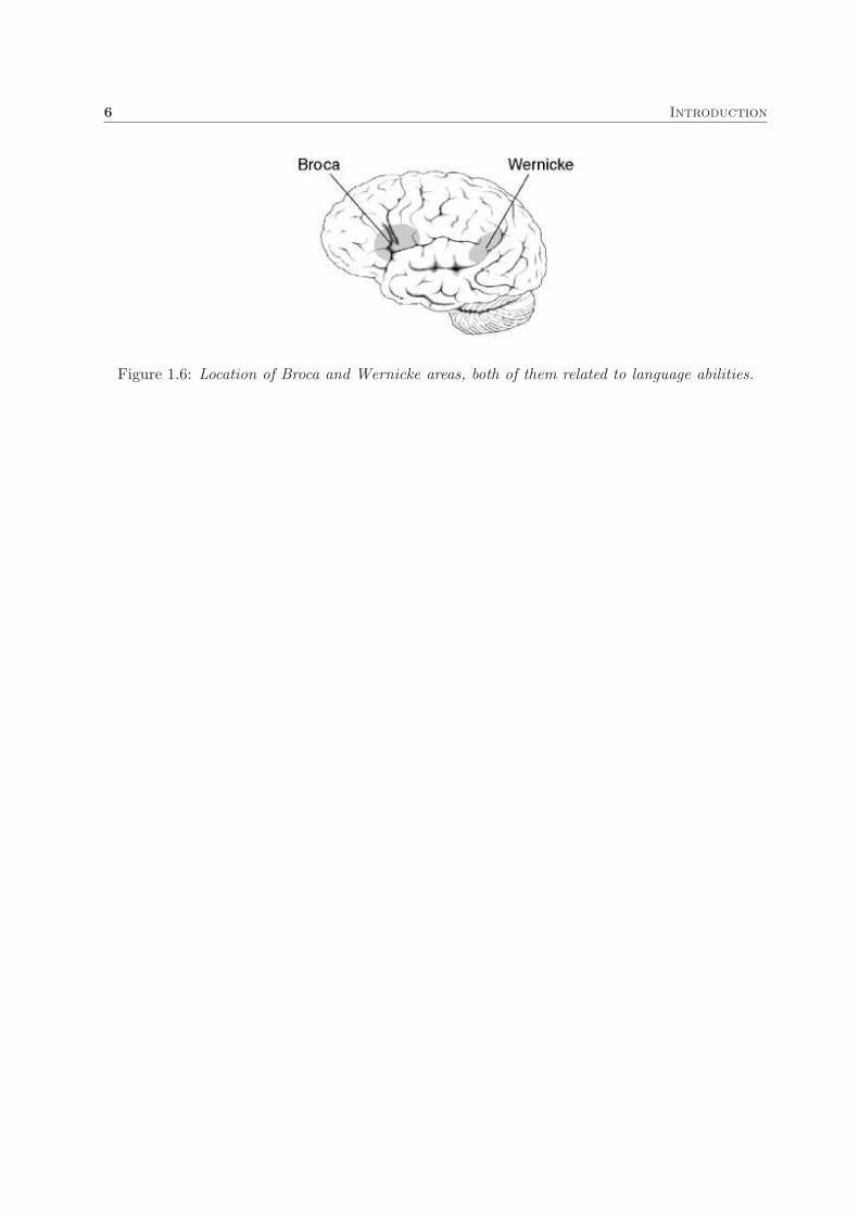
The first language area found within the left hemisphere is called Broca’s area (see Fig. 1.6),
due to Paul Broca’s research. The Broca’s area not only handle getting language out in a motor
sense, but it seems to be more generally involved in the ability to deal with grammar itself, at
least in its more complex aspects. For example, it handles distinguishing a sentence in passive
form from a simpler subject-verb-object sentence.
The second language area to be discovered is called Wernicke’s area (see Fig. 1.6), after Carl
Wernicke’s finding. Although the problem of not understanding the speech of others is known
as Wernicke’s Aphasia, Wernicke’s area is not reduced to speech comprehension. People with
Wernicke’s Aphasia also have impaired the ability of naming things, often producing words that
sound similar, or the names of related things, as if they are having a serious difficulties with their
mental lexicon.
6 Introduction
Figure 1.6: Location of Broca and Wernicke areas, both of them related to language abilities.

Section 1.2 7
1.2. Memory and its different classifications
In psychology, memory is an organism’s ability to store, retain, and subsequently retrieve
information. It can also be understood as a collection of mental abilities that depend on several
systems within the brain [6]. Traditional studies of memory began in the realms of philosophy,
including techniques of artificially enhancing the memory. While in the late nineteenth and early
twentieth century memory was put within the paradigms of cognitive psychology, it has more
recently become one of the key basis of cognitive neuroscience; an emergent field whose role is
being an interdisciplinary link between cognitive psychology and neuroscience [7].
Figure 1.7: The Persistence of Memory. Salvador Dalı. 1931
Memory subtypes can be classified through several ways attending to duration, nature and
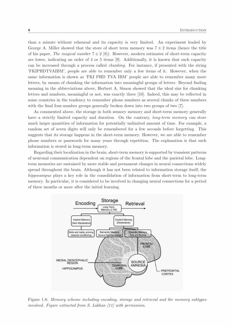
retrieval of information. From an information processing point of view, three main stages char-
acterize the formation and retrieval of memory [7]: encoding or registration (processing and
combining of received information), storage (creation of a permanent record of the encoded infor-
mation) and retrieval or recall (calling back the stored information in response to some cue for
use in a process or activity). See Fig. 1.8 for a schematic representation of these stages.
Memory types based on duration
A widely accepted classification of memory based on the duration of memory retention dis-
tinguish three distinct types of memory: sensory memory, short term memory and long term
memory described below (see [7] for a detailed review).
Sensory memory corresponds approximately to the first 200 - 500 milliseconds once an item
is perceived. An example would be the ability to look at an item for no more than a second and
remember what it looked like. Although sensory registers show a large capacity for unprocessed
information, its duration is very limited and once the stimulus has ended is momentarily hold
accurately and quickly degraded.
Short-term memory, also known as working memory, is believed to rely mostly on an acoustic
code for storing information, and to a lesser extent a visual code. Part of the information in
sensory memory is transferred to short-term memory. It permits to recall something for no more
8 Introduction
than a minute without rehearsal and its capacity is very limited. An experiment leaded by
George A. Miller showed that the store of short term memory was 7 ± 2 items (hence the title
of his paper, The magical number 7 ± 2 [8]). However, modern estimates of short-term capacity
are lower, indicating an order of 4 or 5 items [9]. Additionally, it is known that such capacity
can be increased through a process called chunking. For instance, if presented with the string
’FKIPHDTVAIBM’, people are able to remember only a few items of it. However, when the
same information is shown as ’FKI PHD TVA IBM’ people are able to remember many more
letters, by means of chunking the information into meaningful groups of letters. Beyond finding
meaning in the abbreviations above, Herbert A. Simon showed that the ideal size for chunking
letters and numbers, meaningful or not, was exactly three [10]. Indeed, this may be reflected in
some countries in the tendency to remember phone numbers as several chunks of three numbers
with the final four-number groups generally broken down into two groups of two [7].
As commented above, the storage in both sensory memory and short-term memory generally
have a strictly limited capacity and duration. On the contrary, long-term memory can store
much larger quantities of information for potentially unlimited amount of time. For example, a
random set of seven digits will only be remembered for a few seconds before forgetting. This
suggests that its storage happens in the short-term memory. However, we are able to remember
phone numbers or passwords for many years through repetition. The explanation is that such
information is stored in long-term memory.
Regarding their localization in the brain, short-term memory is supported by transient patterns
of neuronal communication dependent on regions of the frontal lobe and the parietal lobe. Long-
term memories are sustained by more stable and permanent changes in neural connections widely
spread throughout the brain. Although it has not been related to information storage itself, the
hippocampus plays a key role in the consolidation of information from short-term to long-term
memory. In particular, it is considered to be involved in changing neural connections for a period
of three months or more after the initial learning.
Figure 1.8: Memory scheme including encoding, storage and retrieval and the memory subtypes
involved. Figure extracted from S. Lakhan [11] with permission.

Section 1.2 9
Memory types based on information type
Long-term memory is divided into declarative (explicit) and procedural (implicit) memories
[12]. See Fig. 1.8 for a scheme of its structure.
Declarative memory requires conscious recall, in the sense that some conscious process must
call back the information. It is also known as explicit memory, since it consists of information
that is explicitly stored and retrieved. It can be divided into semantic memory, which concerns
facts taken independent of context; and episodic memory, which concerns information specific
to a particular context, such as a time and place. Semantic memory allows the encoding of
abstract knowledge about the world, such as ’Rome is the capital of Italy’. Episodic memory
is used, on the contrary, for more personal memories, such as the sensations, emotions, and
personal associations involving a particular place or time. Their processing include the details
surrounding the memory (i.e., where, when, and with whom the experience took place) and have
to be maintained; otherwise the memory would be semantic (Bullock 1998). For instance, one
may own an episodic memory of humans setting foot on the Moon for the first time, including
watching Neil Armstrong and even the face of a specific journalist announcing it on TV. However,
if the contextual details of this event were lost, the remaining would be only a semantic memory
that humanity went to the Moon. This ability to recall episodic information concerning a memory
is known as source monitoring [13], and is subject to distortion or impairment that can lead to
source amnesia [11] (see section 1.2).
Nevertheless, procedural memory (also known as implicit memory) is based on implicit learning,
instead of on the conscious recall of information. This memory is primarily employed in learning
motor abilities and should be considered a subset of implicit memory. It is revealed when one
does better in a given task due only to repetition, i.e. no new explicit memories have been formed,
but one is unconsciously accessing aspects of previous experiences. In motor learning tasks, it
depends on the cerebellum and basal ganglia.
A table summarizing the differences between declarative memories (semantic memory and
episodic memory) and procedural memory is shown below (see table 1.1).
Memory types based on temporal direction
Another way to characterize memory functions consists of defining whether the content to be
remembered is in the past, retrospective memory, or in the future, prospective memory. Hence
retrospective memory as a category includes semantic and episodic memories. On the contrary,
prospective memory is memory for future intentions, or remembering to remember [14]. Prospec-
tive memory can be divided into event- and time-based prospective remembering. Time-based
prospective memories are triggered by a time-cue, such as visiting a friend (action) at 6pm (cue).
Event-based prospective memories are intentions triggered by cues, such as remembering to make
a phone call (action) after seeing a mobile phone (cue). Cues do not necessarily need to be
related to the action, as the mobile phone example is. Indeed, people usually produce cues
such as sticky-notes, string around the finger or knotted handkerchiefs, as a strategy to enhance
prospective memory [7].
Semantic memory
Semantic memory is a distinct part of the declarative memory system [15] comprising knowl-
edge of facts, vocabulary, and concepts acquired through everyday life [16]. Contrary to episodic
memory, which stores life experiences, semantic memory is not linked to any particular time or

10 Introduction
Table 1.1: Summarization of the three memory systems based on information type: semantic
memory, episodic memory and procedural memory. Table extracted from A.E. Budson and B.H.
Price [6].
.
Memory system Anatomical structures Length of storage Type of awareness Examples
Episodic memory Medial temporal lobes, Minutes to years Explicit, declarative Remembering a short story,
anterior thalamic nucleus what you had for dinner last
mamillary body, fornix, night, what you did on your
prefrontal cortex last birthday
Semantic memory Inferolateral temporal lobes Minutes to years Explicit, declarative Knowing who was the first
president of the U.S., the
color of a lion, and how a
fork differs from a comb
Procedural memory Basal ganglia, cerebellum, Minutes to years Explicit or implicit, Driving a car with a stand-
supplementary motor area ard transmission (explicit),
learning the sequence of
numbers on a phone without
trying (implicit)
place. In a more restricted definition, it is responsible for the storage of semantic categories and
naming of natural and artificial concepts [6]. Regarding its localization, neuroimaging and le-
sion studies suggest the existence of a large distributed organization of semantic representations,
which includes infero-lateral temporal lobe, perception and motion modality regions [6, 17]. For
instance, when thinking about a cow, its visual features are represented in visual areas of the
brain while the sound it makes is stored in auditory areas. However, diseases such as Alzheimer’s
and semantic dementia are known to cause non-dissociated impairments of semantic memory [18],
difficult to explain from a modality-segmented perspective. Therefore it has been argued that
a modality-independent shared core is also needed for establishing high order relations between
concepts [19]. Both diseases but especially semantic dementia damage the temporal lobe [20, 21].
These findings have led to the proposal of semantic storage models where an amodal hub situated
in the temporal lobe is in permanent communication with modality-specific regions [19].
Memory disorders
Memory functioning is vulnerable to a wide variety of different pathologic processes, including
neurodegenerative diseases, strokes, tumors, head trauma, hypoxia, cardiac surgery, malnutrition,
attention-deficit disorder, depression, anxiety, the side effects of medication and normal aging
[22, 23]. Hence memory impairment is commonly observed by physicians of multiple disciplines
such as medicine, psychiatry, surgery and neurology. In many of the disorders, the most often
disabling feature is memory loss (also known as amnesia), which can severely impair the normal
daily activities of the patients [6] (see Fig. 1.8).
Much of the current knowledge of memory has come from studying memory disorders. Loss of
memory is known as amnesia. There are many kinds of amnesia, and by studying their different

Section 1.2 11
Figure 1.9: The Disintegration of the Persistence of Memory. Salvador Dalı. 1954.
forms, it has been possible to observe apparent defects in individual sub-systems of memory, and
thus hypothesize their function in the normally working brain. Other neurological disorders such
as Alzheimer’s disease (AD), Parkinson’s disease, Multiple Sclerosis or schizophrenia can also
affect memory and cognition. Hyperthymesia, or hyperthymesic syndrome, is a disorder which
affects an individual’s autobiographical memory, essentially meaning that they cannot forget small
details that otherwise would not be stored. While not a disorder, a common temporary failure of
word retrieval from memory is the tip-of-the-tongue (TOT) phenomenon. Sufferers of Nominal
Aphasia (also known as Anomia), however, experience the TOT phenomenon on an ongoing basis
due to damage both to the frontal and parietal lobes.

12 Introduction
1.3. Verbal fluency tasks
Verbal fluency tasks based on semantic and phonetic cues are widely used in neuropsychological
assessment [24, 25]. In semantic fluency tasks participants have to produce words from a category
such as animals in a given time (usually 60 or 90 seconds). Although the most common clinical
measure is the number of different words named by each participant [26], it has also been observed
that words tend to appear in semantically grouped clusters [27–30]. This led Troyer et al. [31] to
propose a two component model of the semantic fluency task. The first component, clustering,
implies the production of related words until a particular category is exhausted. The second
component is switching to a different semantic cluster. It has been argued that switching implies
the flexibility to initiate a new category search and is related to frontal executive functioning while
clustering depends on the temporal lobe and is characterized by local explorations of semantic
memory [31–34].
Figure 1.10: Localization of the frontal lobe and the temporal lobe. In semantic verbal fluency
tasks, activity from the former has been associated to switching flexibility (ability to initiate a new
category) while the later has been associated to clustering (production of related words).

Section 1.4 13
1.4. Network theory and exploration phenomena
Network theory is a research area of applied mathematics, physics and graph theory that
has application in a wide spectrum of disciplines. It concerns itself with the study of graphs as a
representation of either symmetric or asymmetric relations (represented by links or edges) between
a set of objects (nodes). In the last decade, it has been used for the modeling and characterization
of a number of complex systems including biological interacting networks [35–39], sociophysics
[40, 41], epidemics [42, 43], the Internet [44, 45] and language [46, 47]. In all cases, systems were
represented as a set of nodes representing individual entities that have certain links that might
represent interactions of different nature (e.g. the case of protein-protein interaction networks)
or communication pathways (e.g. the case of Internet). It has been demonstrated that many of
these real-world networks show properties such as small-world and high clustering properties, and
scale-free (SF) degree distributions [48]. These properties necessarily imply a large heterogeneity
in the connectivity of the nodes and a short average distance between nodes. Theoretical models
have been developed to understand the structure and functions of the underlying real systems.
For example, scale-free networks have been shown to be resilient to random damage [49–51] but
at the same time fragile to intentional attacks on the small set of highly connected nodes (hubs)
[52].
Figure 1.11: Example of a protein-protein interaction network extracted from Goni et al. [38].
Purple nodes are proteins whose genes have been related to Multiple Sclerosis. Red nodes are
proteins that interact with purple nodes and belong to the giant component of the network (biggest
subset of connected nodes). Green nodes also interact with purple nodes but are located in isolated
subsets of the network. Examples of hubs (nodes highly connected) are HLA-DRA, SPTAN1,
ITGA6, UN and ZAP70.
Its wide application has given rise to many different topological measures (see [53, 54] for a
review) in an effort to better understand the architecture of the systems modeled by such networks.
Additionally, dynamical rather than strictly topological measures have acquired a high relevance
in order to understand not only the architecture of a complex system but also its behavior in

14 Introduction
terms of exploration and propagation. While many studies have concentrated on the properties
of, for example, power-law networks and how they are generated, another interesting problem is
to find efficient algorithms for searching or exploring within graphs. Recent papers talk about the
discipline of search research [55]. Here, it is crucial to determine the constraints of the system
under study. Two examples are, in one hand a two dimensional space where a walker (generic
name for an entity that explores a system) aims to find a target, and on the other hand a network
of connected nodes that determines the valid locations (nodes) and valid walks (links between
nodes). Moreover, it is crucial to define whether the walker is aware of the full network and has
memory (conscious of nodes already visited) or not. Hub is a term used to refer to those nodes
which are highly connected in a network. It is easy to imagine using those hubs as preferential
nodes to visit due to their wide variety of targets in order to rapidly reach a specific node.
For example, imagine the case of a traveler using available city to city transports to finally
get to a small and badly connected town. Such traveler is taking advantage of being aware of
the transport structure and the location of different populations to reach a specific target. Let
us assume that this traveler does not know anything about the transport structure (example of
a network) and has no memory (he does not remember the places he has already visited). The
most feasible strategy for him is the so called random-walk, which was previously studied in one
and two dimensional spaces (see Fig. 1.12). It consists of randomly choosing the orientation of
each step done by the walker.
Figure 1.12: Example of a random walk in a two dimensional space. In the limit, for many and
very small steps, what is obtained is the so called Brownian motion, i.e. the random movement
of particles suspended in a liquid or a gas. Figure extracted from Wikipedia [56].
When steps are set to be small and simulation is run for a long time, the trajectories described
are those expected for the movement of particles suspended in a liquid or a gas. In the case
of random-walks in networks, the only difference is that movements are not constraint by near
spatial coordinates but on links of current node indicating the allowed targets for the next step
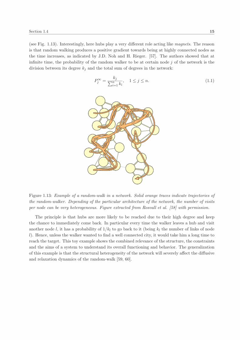
Section 1.4 15
(see Fig. 1.13). Interestingly, here hubs play a very different role acting like magnets. The reason
is that random walking produces a positive gradient towards being at highly connected nodes as
the time increases, as indicated by J.D. Noh and H. Rieger. [57]. The authors showed that at
infinite time, the probability of the random walker to be at certain node j of the network is the
division between its degree kj and the total sum of degrees in the network:
P∞j =
kj∑n
i=1 ki, 1 ≤ j ≤ n. (1.1)
Figure 1.13: Example of a random-walk in a network. Solid orange traces indicate trajectories of
the random-walker. Depending of the particular architecture of the network, the number of visits
per node can be very heterogeneous. Figure extracted from Rosvall et al. [58] with permission.
The principle is that hubs are more likely to be reached due to their high degree and keep
the chance to immediately come back. In particular every time the walker leaves a hub and visit
another node l, it has a probability of 1/kl to go back to it (being kl the number of links of node
l). Hence, unless the walker wanted to find a well connected city, it would take him a long time to
reach the target. This toy example shows the combined relevance of the structure, the constraints
and the aims of a system to understand its overall functioning and behavior. The generalization
of this example is that the structural heterogeneity of the network will severely affect the diffusive
and relaxation dynamics of the random-walk [59, 60].
16 Introduction

17
Chapter 2
Frequency patterns and
heterogeneity of concepts in verbal
fluency
A study of how some concepts are named by more participants and earlier than others and its
implications.
18 Frequency patterns and heterogeneity of concepts in verbal fluency
2.1. The experimental dataset of verbal fluency
Two hundred subjects, healthy Spanish speakers, were recruited (83 males, 117 females).
Participants ranged from 18 to 61 years (mean=31.8, SD= 11.75) and their education ranged
from 5 to 30 years (mean=15.2, SD= 3.85). Participants were asked to name all the animals they
could in 90 seconds and responses were transcribed to a text file. Every word was converted to
its singular and three pure synonyms were unified. Finally, one word that was not an animal was
removed.
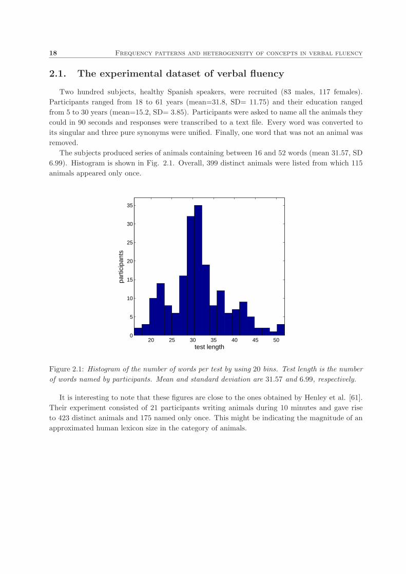
The subjects produced series of animals containing between 16 and 52 words (mean 31.57, SD
6.99). Histogram is shown in Fig. 2.1. Overall, 399 distinct animals were listed from which 115
animals appeared only once.
20 25 30 35 40 45 500
5
10
15
20
25
30
35
test length
part
icip
ants
Figure 2.1: Histogram of the number of words per test by using 20 bins. Test length is the number
of words named by participants. Mean and standard deviation are 31.57 and 6.99, respectively.
It is interesting to note that these figures are close to the ones obtained by Henley et al. [61].
Their experiment consisted of 21 participants writing animals during 10 minutes and gave rise
to 423 distinct animals and 175 named only once. This might be indicating the magnitude of an
approximated human lexicon size in the category of animals.
Section 2.2 19
2.2. Frequency distribution of words
Power-law and exponential distributions
A finite sequence of real numbers y = {y1, y2, ..., yn} ordered in such a way that y1 ≥ y2 ≥
... ≥ yn, is said to follow a power-law or scaling relationship when it satisfies:
k = cy−γk , (2.1)
where k is the rank of yk, c is a constant and γ is the scaling index. In these kind of distribu-
tions, the relation between the rank k and y is linear (with slope equals to −γ) when plotted on
log-log scale. The reason is that expression of equation (2.1) can be rewritten as
log(k) = log(c) − γlog(yk), (2.2)
after taking logarithms on both sides.
Assuming a probability model P for a non negative random variable X, its cumulative distri-
bution function (CDF) is defined as
F (x) = P [X ≤ x], x ≥ 0, (2.3)
and hence, the complementary CDF, F (x) is defined as
F (x) = 1 − F (x) = P [X > x], x ≥ 0. (2.4)
A random variable X or its corresponding distribution F is said to follow a power-law with index
γ when
P [X > x] ≈ cx−γ , γ > 0. (2.5)
If the derivative of the cumulative distribution function F (x) exists, then f(x) = ddx
F (x) is
called the probability density function of X. This implies that the stochastic cumulative form
of scaling or size-rank relationship described in equation (2.5) has a non cumulative equivalency
defined as
f(x) ≈ cx−(1+γ), (2.6)
which also appears as a line (slope equals −(1 + γ)) on a log-log scale. Nevertheless, the use of
this non cumulative approach has been a source of mistakes in the analysis and interpretation of
real data and in general is recommended to be avoided [62].
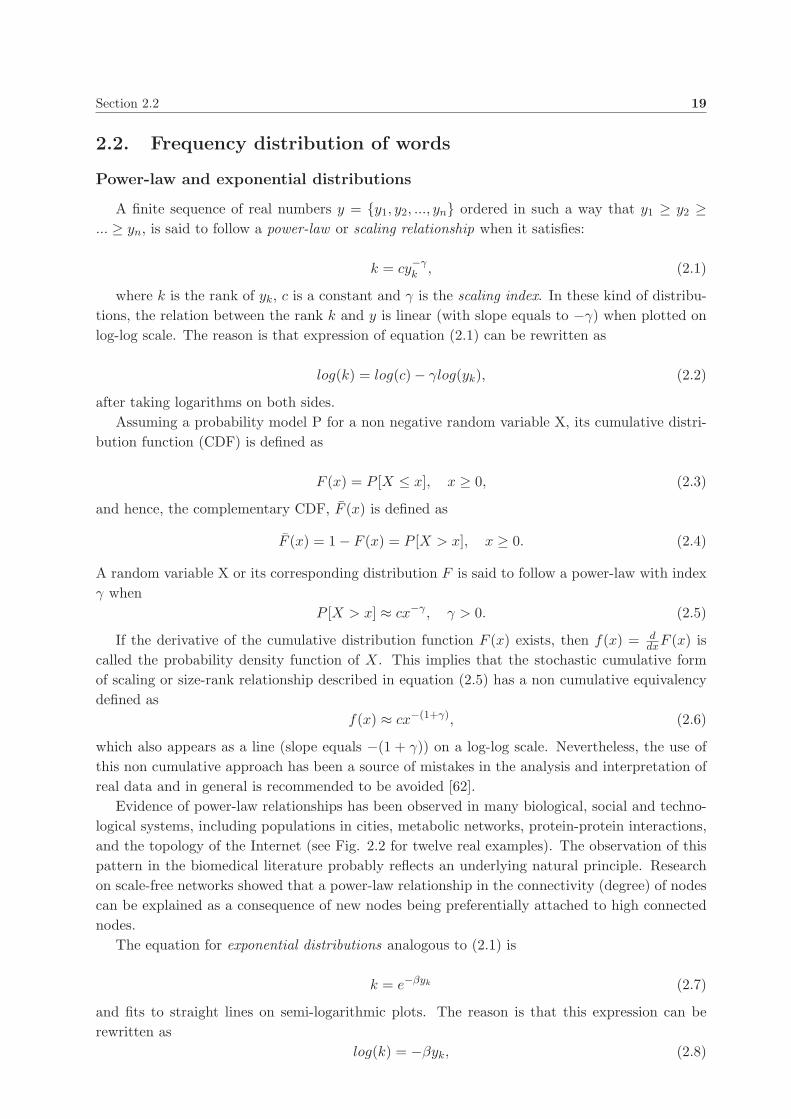
Evidence of power-law relationships has been observed in many biological, social and techno-
logical systems, including populations in cities, metabolic networks, protein-protein interactions,
and the topology of the Internet (see Fig. 2.2 for twelve real examples). The observation of this
pattern in the biomedical literature probably reflects an underlying natural principle. Research
on scale-free networks showed that a power-law relationship in the connectivity (degree) of nodes
can be explained as a consequence of new nodes being preferentially attached to high connected
nodes.
The equation for exponential distributions analogous to (2.1) is
k = e−βyk (2.7)
and fits to straight lines on semi-logarithmic plots. The reason is that this expression can be
rewritten as
log(k) = −βyk, (2.8)
20 Frequency patterns and heterogeneity of concepts in verbal fluency
100
102
104
10−5
10−4
10−3
10−2
10−1
100
P(x
)
(a)
100
101
102
10−4
10−3
10−2
10−1
100
(b)
100
101
102
103
10−4
10−2
100
(c)
metabolic
100
102
104
10−5
10−4
10−3
10−2
10−1
100
P(x
)
(d)
Internet
100
102
104
106
10−6
10−4
10−2
100
(e)
calls
words proteins
100
101
102
103
10−2
10−1
100
(f)
wars
100
102
104
10−5
10−4
10−3
10−2
10−1
100
P(x
)
(g)
terrorism
102
104
106
108
10−6
10−4
10−2
100
(h)
100
101
102
10−3
10−2
10−1
100
(i)
species
100
102
104
106
10−3
10−2
10−1
100
x
P(x
)
(j)
103
104
105
106
107
10−3
10−2
10−1
100
x
(k)
106
107
10−3
10−2
10−1
100
x
(l)
HTTP
birds blackouts book sales
Figure 2.2: The cumulative distribution functions P (x) = P [X > x] (blue circles) and their
maximum likelihood power-law fits (dashed black lines), for 12 empirical data sets of different
nature. Figure extracted from Clauset et al. [63] with permission.

Section 2.2 21
after taking logarithms on both sides. Hence for a random variable X, the equation analogous to
(2.5) is
P [X > x] ∼ e−βx β > 0. (2.9)
There has been also evidence of exponential relationships in different fields such as psychology
[64] (see Fig. 2.3) and physiology [65].
Figure 2.3: Examples of exponential decays in psychology. Figure extracted from Shepard et al.
[64].
Fitting our data
We modeled the distribution P [X > x] for the variable frequencies of words (named in the
animals semantic verbal fluency tests) as a power-law and exponential distributions by means of
the lest square method. The goodness of fit for each approach was measured by R2. It measures
the fraction of the total squared error that is explained by the model. In our case, it is the fraction
between the actual data and those points in the linear model for the log-log plot (for the power-
law evaluation) and the linear-log plot (for the exponential evaluation). In the case of evaluating

22 Frequency patterns and heterogeneity of concepts in verbal fluency
linear models, R2 numerically matches with the square of Pearson correlation coefficient. For the
general case, its definition is:
R2 = 1 −SSerr
SStot= 1 −
∑
i(yi − y′i)2
∑
i(yi− < y >)2(2.10)
where values yi are the observed ones, < y > their averaged value and y′i the predicted ones
according to the model.
The results plotted in Fig. 2.4 show that the frequency distribution of words is much closer
to an exponential distribution than to a power-law distribution. The plot of the data shows that
most of the words are rarely said while a very small amount appears in many tests. In particular,
only 9 words corresponding to 9 prototypical animals were said by more than 50 percent of the
participants. They were, in decreasing order of frequency: dog, cat, lion, elephant, giraffe, whale,
tiger, horse and cow.
100
101
102
10−2
10−1
100
101
x
P[X
>x]
word frequencies
power−law (R2=0.41)
exponential (R2=0.93)
Figure 2.4: R2 measurements for power-law and exponential models show that frequency of words
is much closer to the latter. Figure axes are log-log and thus data would have been much more
linearin the case of a power-law.
In natural language it is well known that frequency distribution follows a decay with γ = 2,
this is known as the Zipf’s law [66, 67]. However, it is noticeable that this situation is quite
different to word retrieval. A priori, two characteristics of fluency tasks might have explained
such difference in the distribution of word frequencies between natural language and verbal fluency.
One would have been the presence of only nouns in verbal fluency tests, but it has been reported
that frequency of nouns in natural language follows an exponent close to 2 as well [67]. The
second and more plausible explanation is the almost complete absence of word repetitions in

Section 2.2 23
verbal fluency. When there is no limit on repetitions, the difference in use between frequent
and rare words is probably magnified, leading to an even more abrupt differences and decay. A
detailed table including the frequency and averaged position within verbal fluency tests of every
word can be seen at Appendix A.

24 Frequency patterns and heterogeneity of concepts in verbal fluency
2.3. Word position and word heterogeneity rate
It has been reported that in semantic verbal fluency, frequent words and therefore prototypical
concepts are named not only more frequently but also earlier in the tests [68, 69]. Such result has
been noticed in many tests dealing with different categories, for instance the tools category [70].
We correlated word frequencies and their averaged position within the tests and again found a
large negative correlation (Pearson correlation coefficient, r = −0.80, p < 10−16) that is shown in
Fig. 2.5. Therefore, frequency of a word is an accurate indicator of its expected averaged position
within the tests.
0 0.2 0.4 0.6 0.8 10
5
10
15
20
25
word frequency
aver
aged
wor
d po
sitio
n
r = −0.80p < 0.05
Figure 2.5: Word frequencies compared to their averaged position within the tests. A large negative
correlation is found indicating that the frequency of a word is an accurate indicator of its expected
position within the tests.
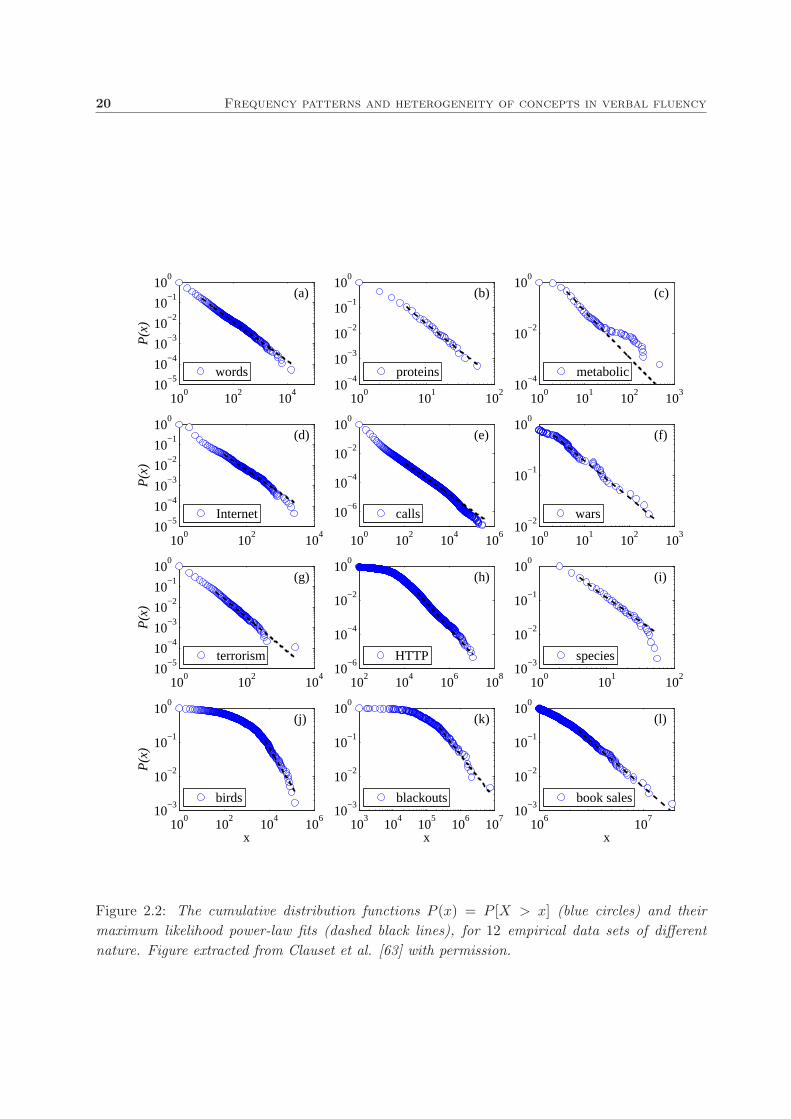
Nevertheless, a non answered question is how such frequency decay is and whether the fre-
quency drop remains thereafter. To assess this phenomenon we made the experiment the other
way around, i.e., we correlated the word positions within the test with the averaged frequency
of those words in the whole dataset. Let us note that, as shown in section 2.1, participants said
different numbers of words. Hence the averaged frequency evaluated at every position was done
by taking into account only those participants that reached that test length. Results are shown
in Fig. 2.6. A cubic interpolation fitted the data accurately. Results illustrate the presence of
three different stages: a decay on saying the most frequent words at the beginning (1st to 22nd
position) followed by a plateau region of medium frequency words (23rd to 35th position) during
the middle stage and a final decay (36th to 52nd position) where the least frequent words are
named.
In order to evaluate concept heterogeneity for a given test section, we defined the measurement
of word heterogeneity word rate (WHR). It consists of the quotient between the number of different
word instances and the total number of word instances for a particular section or stage.

Section 2.3 25
Let us denote by W = {w1, w2, ..., wn} the list of all the animals (with no repetitions) said by
the N = 200 participants. Hence the number of distinct instances said in a particular section of
the test (positions from a to b) can be expressed by∑n
i=1 k(wi, a, b) where
k(wi, a, b) =
{
1 if at least one participant said wi within a and b positions of his test
0 otherwise.(2.11)
Furthermore, the total number of animals (repeated or not) said by participants in a specific
section of the test (positions from a to b) can be expressed by∑n
i=1 f(wi, a, b) where
f(wi, a, b) = number of participants that said wi within a and b positions. (2.12)
Notice that f(wi, a, b) is not equal to (b − a)N since participants do not necessarily get to say
b words. Finally, we define word heterogeneity rate (WHR) as the division between distinct
instances and total instances within a section [a,b] of the tests as:
WHR(a, b) =number of distinct instances
total number of instances=
∑ni=1 k(wi, a, b)
∑ni=1 f(wi, a, b)
. (2.13)
The range of values goes from 1M
to 1, being M the total number of participants. The former
occurs when participants say the same set of words in any order in a given section (minimum
WHR). The latter occurs when participants say all words different to each other in a given section
(maximum WHR).
Results show (see Fig. 2.6) that such heterogeneity increases along the test (WHRstage1 =
0.07, WHRstage2 = 0.18 and WHRstage3 = 0.53) indicating that participants share a strong
preference for naming a small set of concepts at the beginning that is gradually lost as the test
advances, giving rise to many more but less frequent animals in stage3.
Summarizing, two patterns have been shown here. First, the animals named frequently tend to
appear at the beginning and second, the heterogeneity among participants when naming animals
increases along the test. Since every word retrieved is due to either switching or clustering, there
must be at least one of these mechanisms producing this phenomenon. This question will be
assessed in the next chapter.
26 Frequency patterns and heterogeneity of concepts in verbal fluency
10 20 30 40 500
0.1
0.2
0.3
0.4
0.5
0.6
0.7
word position
aver
aged
wor
d fr
eque
ncy
data
cubic interp.
stage3WHR=0.53
stage1WHR=0.07
stage2WHR=0.18
Figure 2.6: Mean word frequency plotted as a function of word position in the tests. Continuous
line is the cubic interpolation that explains the phenomenon by identifying three different stages:
a decay after saying the most frequent words, a plateau region where words with medium frequency
are said and a final decay with the least prototypical words. WHR stands for heterogeneity word
rate and represents the proportion of different words named at each stage.
27
Chapter 3
Conceptual network topology and
switching-clustering differential
retrieval
An unsupervised approach towards the understanding of the organization and retrieval of
concepts based on network theory and verbal fluency tasks.
28 Conceptual network topology and switching-clustering differential retrieval
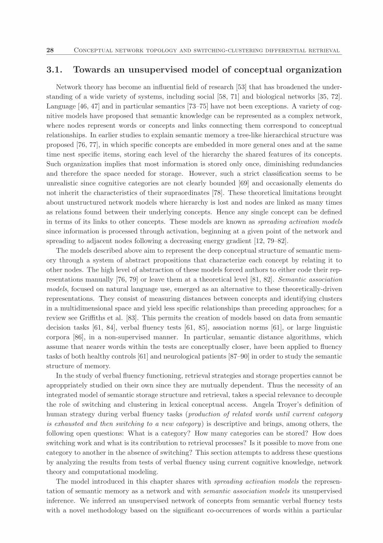
3.1. Towards an unsupervised model of conceptual organization
Network theory has become an influential field of research [53] that has broadened the under-
standing of a wide variety of systems, including social [58, 71] and biological networks [35, 72].
Language [46, 47] and in particular semantics [73–75] have not been exceptions. A variety of cog-
nitive models have proposed that semantic knowledge can be represented as a complex network,
where nodes represent words or concepts and links connecting them correspond to conceptual
relationships. In earlier studies to explain semantic memory a tree-like hierarchical structure was
proposed [76, 77], in which specific concepts are embedded in more general ones and at the same
time nest specific items, storing each level of the hierarchy the shared features of its concepts.
Such organization implies that most information is stored only once, diminishing redundancies
and therefore the space needed for storage. However, such a strict classification seems to be
unrealistic since cognitive categories are not clearly bounded [69] and occasionally elements do
not inherit the characteristics of their supraordinates [78]. These theoretical limitations brought
about unstructured network models where hierarchy is lost and nodes are linked as many times
as relations found between their underlying concepts. Hence any single concept can be defined
in terms of its links to other concepts. These models are known as spreading activation models
since information is processed through activation, beginning at a given point of the network and
spreading to adjacent nodes following a decreasing energy gradient [12, 79–82].
The models described above aim to represent the deep conceptual structure of semantic mem-
ory through a system of abstract propositions that characterize each concept by relating it to
other nodes. The high level of abstraction of these models forced authors to either code their rep-
resentations manually [76, 79] or leave them at a theoretical level [81, 82]. Semantic association
models, focused on natural language use, emerged as an alternative to these theoretically-driven
representations. They consist of measuring distances between concepts and identifying clusters
in a multidimensional space and yield less specific relationships than preceding approaches; for a
review see Griffiths et al. [83]. This permits the creation of models based on data from semantic
decision tasks [61, 84], verbal fluency tests [61, 85], association norms [61], or large linguistic
corpora [86], in a non-supervised manner. In particular, semantic distance algorithms, which
assume that nearer words within the tests are conceptually closer, have been applied to fluency
tasks of both healthy controls [61] and neurological patients [87–90] in order to study the semantic
structure of memory.
In the study of verbal fluency functioning, retrieval strategies and storage properties cannot be
aproppriately studied on their own since they are mutually dependent. Thus the necessity of an
integrated model of semantic storage structure and retrieval, takes a special relevance to decouple
the role of switching and clustering in lexical conceptual access. Angela Troyer’s definition of
human strategy during verbal fluency tasks (production of related words until current category
is exhausted and then switching to a new category) is descriptive and brings, among others, the
following open questions: What is a category? How many categories can be stored? How does
switching work and what is its contribution to retrieval processes? Is it possible to move from one
category to another in the absence of switching? This section attempts to address these questions
by analyzing the results from tests of verbal fluency using current cognitive knowledge, network
theory and computational modeling.
The model introduced in this chapter shares with spreading activation models the represen-
tation of semantic memory as a network and with semantic association models its unsupervised
inference. We inferred an unsupervised network of concepts from semantic verbal fluency tests
with a novel methodology based on the significant co-occurrences of words within a particular

Section 3.1 29
class, in our case, animals. This network allowed us to study lexical organization and specifically
the existence of semantic modularity and was later used as an in-silico evaluator of switching and
clustering events. Such evaluation together to the definition of two measurements (accessibility
and diffusivity) allowed us to decouple switching and clustering retrieval mechanisms based on
empirical findings.
For the purpose of this study we chose to test verbal fluency using the category of animals.
In particular we used the empirical dataset described in Section 2.1. Although other semantic
categories have been used in these kind of tests, animals have the advantage of universality: it
is a clear enough test across languages and cultures with only minor differences across different
countries, educational systems and age or generation [25]

30 Conceptual network topology and switching-clustering differential retrieval
3.2. Unsupervised generation of a conceptual network
Verbal fluency tests
The dataset containing 200 semantic verbal fluency tests (animals) studied here is the same
one described in Section 2.1.
Inference of concept co-occurrences
The first aim was to extract relations between concepts based on test evidences in order to
obtain a conceptual network (CN). For this we assumed that a relationship between 2 words
existed when their rate of co-occurrence was significantly higher than expected by chance. The
known high rate of switching in fluency tests, averaged as 0.48 by A. Troyer [31], indicates that
two consecutive words are not necessarily related. Therefore the use of a statistical methodology
rather than an approach based on number of co-occurrences seems to be critical to discern which
concepts are associated. Methodologies based on co-occurrences have been used to study language
networks [91] where the syntactic constraints severely reduce the order of the items.
Let us extend the definition of co-occurrence to the event of two words being distanced or
separated by no more than l−1 words within a test. Hence parameter l defines the window length
for considering co-occurrences, being l = 1 for consecutive words. The reason for increasing the
window length is that we expect to obtain useful information on the relationships of a word not
only from their adjacent words but also from other nearby neighbors. See Fig. 3.1 for an example
of l = 2.
Figure 3.1: Example of window length when l = 2, as done in the present work. The word sequence
represents part of an individual test. When analyzing shark relationships, neighbors distanced no
more than 2 words on both sides are taken into account. Hence in this toy example tiger and whale
on the left and dolphin and tuna on the right co-occurred with shark and thus are shark-related
candidates.
Given the complete set of distinct words {w1, w2, ..., wn} named in the verbal fluency tests, the
expression for the probability of two words (wi,wj) happening together at random is denoted by
(P togetherwi,wj ). It is given by the probability of being in the same test (P test
wi,wj) and window (P lwindow
wi,wj)
by chance.
When assuming that words happen whithin tests at random, the probability of a word wi to
occur in a test is independent of the rest of the test and corresponds to a Bernoulli variable with
parameter Pwi, denoted by
Pwi=
fwi
M, (3.1)
where fwiis the frequency of wi within the tests and M is the number of tests (200 in our case).
Therefore the probability of two words being in the same test by chance, P testwi,wj
, is also de-
termined by the product of two Bernoulli variables that occur independently. Their rates of
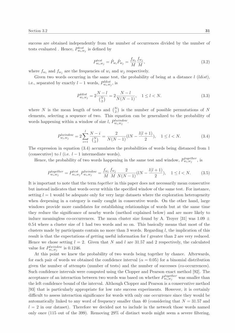
Section 3.2 31
success are obtained independently from the number of occurrences divided by the number of
tests evaluated . Hence, P testwi,wj
is defined by
P testwi,wj
= PwiPwj
=fwi
M
fwj
M, (3.2)
where fwiand fwj
are the frequencies of wi and wj respectively.
Given two words occurring in the same test, the probability of being at a distance l (ldist),
i.e., separated by exactly l − 1 words, P ldistwi,wj
, is
P ldistwi,wj
= 2N − l(
N2
) = 2N − l
N(N − 1), 1 ≤ l < N. (3.3)
where N is the mean length of tests and(
N2
)
is the number of possible permutations of N
elements, selecting a sequence of two. This equation can be generalized to the probability of
words happening within a window of size l, P lwindowwi,wj
.
P lwindowwi,wj
= 2l
∑
i=1
N − i(
N2
) =2
N(N − 1)(lN −
l(l + 1)
2), 1 ≤ l < N. (3.4)
The expression in equation (3.4) accumulates the probabilities of words being distanced from 1
(consecutive) to l (i.e. l − 1 intermediate words).
Hence, the probability of two words happening in the same test and window, P togetherwi,wj , is
P togetherwi,wj
= P testwi,wj
P lwindowwi,wj
=fwi
M
fwj
M
2
N(N − 1)(lN −
l(l + 1)
2), 1 ≤ l < N. (3.5)
It is important to note that the term together in this paper does not necessarily mean consecutive
but instead indicates that words occur within the specified window of the same test. For instance,
setting l = 1 would be adequate only for very large datasets where the exploration heterogeneity
when deepening in a category is easily caught in consecutive words. On the other hand, large
windows provide more candidates for establishing relationships of words but at the same time
they reduce the significance of nearby words (method explained below) and are more likely to
induce meaningless co-occurrences. The mean cluster size found by A. Troyer [31] was 1.09 ±
0.54 where a cluster size of 1 had two words and so on. This basically means that most of the
clusters made by participants contain no more than 3 words. Regarding l, the implication of this
result is that the expectations of getting useful information for l greater than 2 are very reduced.
Hence we chose setting l = 2. Given that N and l are 31.57 and 2 respectively, the calculated
value for P lwindowwi,wj
is 0.1246.
At this point we knew the probability of two words being together by chance. Afterwards,
for each pair of words we obtained the confidence interval (α = 0.05) for a binomial distribution
given the number of attempts (number of tests) and the number of successes (co-occurrences).
Such confidence intervals were computed using the Clopper and Pearson exact method [92]. The
acceptance of an interaction between two words was based on whether P togetherwi,wj was smaller than
the left confidence bound of the interval. Although Clopper and Pearson is a conservative method
[93] that is particularly appropriate for low rate success experiments. However, it is certainly
difficult to assess interaction significance for words with only one occurrence since they would be
automatically linked to any word of frequency smaller than 40 (considering that N = 31.57 and
l = 2 in our dataset). Therefore we decided not to include in the network those words named
only once (115 out of the 399). Removing 29% of distinct words might seem a severe filtering,

32 Conceptual network topology and switching-clustering differential retrieval
Table 3.1: Four examples of the concept-concept statistical analysis to decide whether each pair
is associated and thus their nodes are linked in the network. Pair of concepts indicates the pair
studied; Pw1is the frequency of the first word (as defined in equation (3.1); Pw2
is the frequency
of the second word (as defined in equation (3.2)); P togetherw1,w2
is the value obtained according to
equation (3.5); hits is the number of times that both words were named within a distance not
greater than 2 (parameter l, see equation (3.3)); interval is the confidence interval (α = 0.05) for
the binomial distribution considering the number of hits and the number of attempts (number of
tests); a pair is only linked when P togetherw1,w2
is on the left of the interval, i.e., we can reject that
their words co-occurred by chance.
Pair of concepts Pw1Pw2
P togetherw1,w2
hits interval linked
monkey-horse 0.34 0.51 0.022 2 [0.0012,0.035] no
whale-mouse 0.59 0.45 0.033 6 [0.011,0.064] no
viper-cobra 0.045 0.045 2.52e − 04 4 [0.0055,0.0504] yes
lion-tiger 0.73 0.59 0.054 91 [0.38,0.52] yes
but they only represented 2% of all word occurrences within the tests as they were the least
frequent items. Such small reduction of evidences is indeed one step ahead of previous works
where semantic distance approaches have been applied to those words either said by a minimum
of around 30% of participants or to most named words (threshold set around 12) [61, 87–90].
Summarizing, we defined interacting words as those said by more than one participant that
were found together much more frequently than expected by chance. Those words with no
significant interactions were not included in the network (47 words) since they represented isolated
words that prevent a network analysis and a clustering approach. Additionally, the isolated pair
eel-elver was also removed for the same reason leaving a total of 236 nodes in the network.
The numerical representation of the inferred conceptual network (CN) is a binary symmetric
matrix, the so called adjacency matrix, Acn = [aij ]. Such matrix is square (236x236 in our case)
and contains all possible interactions among words. For every significant relationship between
two words (wi, wj), the positions acnij and acn
ji were set to 1, and 0 otherwise.
The conceptual network
We used this statistical approach described in Section 3.2 to infer concept-concept associations
from verbal fluency tests, taking into account the number of participants, mean test length, win-
dow length and word frequencies. Overall 611 significant concept-concept associations were found.
The output of this method is an adjacency matrix of the CN denoted by Acn = [acnij ]. Fig 3.2
shows the plot of such matrix and Fig.3.3 the visual representation of the network including those
links. This matrix is symmetric (every entry acnij equals acn
ji ) since concept-concept associations
are allowed in both directions and thus links are not oriented. The topological characteristics of
such network and its cognitive and semantic implications are described in Table 3.3 of Section
3.4.

Section 3.2 33
1 50 100 150 200 236
1
50
100
150
200
236
Figure 3.2: Plot of Acn = [acnij ], the adjacency matrix of CN. Those acn
ij positions painted in blue
stand for significant concept-concept relationships found. Overall 611 associations were found
among the 236 animals studied
bee
bumblebee
mite
eaglegolden eagleharrier
scorpion2
moose
clam
anchovy
antelope
spider
squirrel
herring
donkey2
tuna
ostrich
wasp
codwhale
barbsea bream
bison
boa
European lobster
skipjack tuna
ox
edible crab
buffalo
owl
vulture
donkey
sea horse
horse
goat
Goat-kid
cockatoo
sperm whale
alligator
squid
chameleon
camel
canary
crab
kangaroo
snail
caribou
male sheep
carp
rattle snake
zebra
spider crab
pig
common kestrel
jackal
chimpanzee
centipede
deer
Norway lobster cicada
stork
swan
guinea pig
cobra
crocodile
quail
weasel
condor
rabbit
conger
lamb
cormorant
roe deer
coyote
cockroach
crowlittle snake
dolphin
hilt-head bream
dromedary
elephant
elephant seal
echidna
hedgehog
beetle
scorpionstarfish
seal
gazelle
hen
cock
prawn
fallow deer
goose
tick
cat
sparrow hawk
seagull
swallow
gorilla
small pig
sparrow
cricket
cheetah
wormsilkworm
falcon
hamster
hyenahippopotamus
ant
ferret
iguana
wild boar
jaguar
goldfinch
giraffekiwi
koala
wall lizardlizard
lobsterking prawn
barn owl
sole
lion
sea lion
leopard
dragonfly
hare
lynx
llama
wolf
earthworm
true parrot
sea bass
glow-worm
northern pike
macaque
mammut
manatee
praying mantis
butterfly
ladybirdjellyfish
mussel
hake
grouper
kite
monkey
walrus
flymosquito
mouflon
mule
velvet crab
gnu
otter
domestic goose
oranguOrange
killer whale
platypus
caterpillar
bear
anteater
panda
brown bear
polar bear
oyster
sheep
birdpigeon dove
panther
parrot
duck
turkey
peacock
pelican
barnacle
partridge
budgerigar
dog
European robin
fish
swordfish
flatfish
manta ray
hammer fish
magpie2
penguin
louse
piranha
python
chicken
pony
colt
porcupine
flea
octopus
puma
bearded vulturefrog
monkfish
rat
mouse
ray fish
chamois
reindeer
rhinoceros
turbot
nightingale
salamander
gecko
Orange
grasshopper
toad
sardine
cuttlefish
snake
horsefly
badger
calf
shark
tiger
mole
bull
turtle
trout
toucan
capercaillie
cow
European green finch
viper
mare
fox
Pajek
Figure 3.3: The conceptual network (CN) including 236 animals and the 611 associations found
among them. Size of nodes is ranked in 6 intervals and denotes the frequency of their concepts.

34 Conceptual network topology and switching-clustering differential retrieval
3.3. Modularity of the conceptual network
The GTOM algorithm
It is widely accepted that semantic memory in general and natural categories in particular must
be organized in subcategories. However, which and how many these subcategories are remain
poorly understood. From a network perspective, the presence of such categorical organization
should be related to the presence of modules in CN. Therefore our next aim was to study the
existence of modularity and, if present, its fundamentals and a characterization of each module.
Network partitioning in modules provides information about the organization of a system
and the basis of its structure, and is one of the major current topics of interest in the field of
network theory [94, 95]. Performing a hierarchical clustering on the adjacency matrix and setting
a threshold in the dendrogram is among the most basic and common approaches used to find
modules. Nevertheless it must be acknowledged that inferred adjacency matrices from empirical
data (as done in Section 3.2) are often noisy or incomplete, which severely affects hierarchical
clustering evaluation and misleads the selection of an accurate cutoff value for modules detection.
In this context, the generalized topological overlap measure (GTOM) [96] is a generalization or
extension of the topological overlap measure (TOM) [97] based on the selection of higher-order
neighborhoods that can give rise to a more robust and sensitive measure of interconnectedness
that eases the selection of a cutoff in dendrograms. Thus, the evaluation of different high-order
neighborhoods with GTOM is an accurate alternative for finding modules in networks based on
empirical evidences that we used on our adjacency matrix to assess the presence of modules.
Although this method was originally applied to gene expression data, it is a general purpose
method that we applied here on a psychological dataset.
The basis of GTOM is to take into account the number of m-step neighbors that every pair
of nodes share in a normalized fashion. For instance, selecting m = 1 is exactly TOM algorithm
which measures the overlap coefficient OTOM for every pair of nodes i and j,
OTOM (i, j) =J(i, j)
min(ki, kj), (3.6)
where J(i, j) is the number of neighbors shared by nodes i and j, and min(ki, kj) is the min-
imum degree (i.e. number of neighbors) of both nodes. However, setting m = 2 (GTOM2)
consists of considering not only the neighbors shared by every two nodes but also the neighbors
of those neighbors. Therefore the generalization to GTOM can be carried out by growing node
neighborhoods adding links between those nodes distanced no more than m links in the original
adjacency matrix before computing the overlap measure (see equation (3.6)). For any m value,
GTOM output is an overlap matrix with values between 0 and 1 containing interconnectedness
shared information for every pair of nodes. Although there is a lack of numerical methods for
module detection, the information regarding modularity provided by this matrix is the presence
or absence of discrete blocks along the diagonal. Indeed, to get a feasible partition of the network
in modules, the selection of a hierarchical clustering cutoff (0.58 in our data) must separate those
blocks as best as possible. For this analysis we developed a freely available implementation of
GTOM [98]. Finally, the hierarchical clustering was performed on GTOM output matrix with
average criteria.

Section 3.3 35
Modularity analysis of the conceptual network
An evaluation of different GTOM orders (from 1 until 3) shown in Fig. 3.4 indicated that
modules of the network were better retrieved by means of GTOM2 (i.e. one step of expansion
before saturation). At this level of expansion several black boxes emerged along the diagonal
indicating that this is the most accurate generalization level for modules identification of CN
network. It is important to remark that in the case of networks with no implicit modularity
(e.g. random networks), saturation directly emerges in absence of intermediate steps showing
modularity as it can bee seen in figure 3.6
GTOM1 GTOM3GTOM2
Figure 3.4: Generalized topological overlap measure (GTOM) for different levels of growing neigh-
borhoods. GTOM1 corresponds to TOM and do not perform a neighborhood expansion. GTOM2
includes one neighborhood expansion and shows strong evidences of modularity in the form of black
boxes along the diagonal. GTOM3 includes two neighborhood expansions and shows a saturation
of the algorithm.
The obtained overlap measure matrix with GTOM2 is represented at Fig. 3.7. On the top
of the figure, we can see the hierarchical clustering performed on this matrix and the resulting
modules colored. Once modules were defined, its content was qualitatively analyzed to report a
brief description as inclusive as possible of each module and the number of outliers per group.
Table 3.2 contains the 18 modules found and their characteristics. Overall we found that 216 out of
the 236 animals (92%) fitted well in their module characterization based on simple categorizations.
In other words, only 8% of the animals were cataloged as semantic outliers because it seemed
hard to justify semantically their module membership. There are two different reasons that could
explain those semantic outliers: 1 - true but hard to identify or describe semantic features, 2 -
methodological biases such as either false positive interactions in the network and inappropriate
clustering cutoff for certain specific animals that could be reduced increasing the number of
participants. An example of type 1 is the presence of wild boar in Cervidae module. Although it
obviously does not belong to Cervidae, it has many features in common with the Cervidae family
such as habitat or being typical human hunting preys. Examples of type 2 are otter within the
Apes module or edible crab within Insects and Arachnids. Similarly the two smallest modules
were unclassifiable and very likely their components belong to one of the remaining 16 modules.
In summary, we obtained the presence of 16 modules in an unsupervised manner (Fig. 3.7).
The qualitative analysis of these modules confirmed that they were semantic in nature, contained
elements with common attributes and their size was heterogeneous.

36 Conceptual network topology and switching-clustering differential retrieval
Pajek
Figure 3.5: Random network with the same number of nodes and links than CN (236 and 611
respectively). As expected, there was no evidence of modularity even though the same visualization
algorithm that aims to emphasize modularity was used.
Figure 3.6: Generalized topological overlap measure (GTOM) for different levels of growing neigh-
borhoods for a random network with the same nunber of nodes and links than CN. As expected,
there is no evidence of modularity for any neighborhood expansion.

Section 3.3 37
Figure 3.7: GTOM2 overlapping matrix of CN network in grey scale with a hierarchical clustering
on it. Modules obtained correspond to the presence of black blocks along the diagonal of the matrix.
On the left, a qualitative description of each module is also included. The two smallest modules
happened to be unclassifiable and they probably belong to other existing modules.
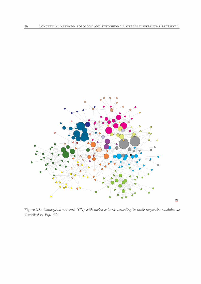
38 Conceptual network topology and switching-clustering differential retrieval
Pajek
Figure 3.8: Conceptual network (CN) with nodes colored according to their respective modules as
described in Fig. 3.7.

Section 3.3 39
Table 3.2: Description of the modules obtained by the GTOM2 technique applied to the CN
network. Id stands for module position in the dendrogram; n is the number of nodes contained
in each module; Explored by is the percent of participants that named at least one concept of
the module; σmodule is the standard deviation of concept frequencies of each module while Most
frequent is the most cited concept; Outliers are the number of concepts that remained semantically
unexplained with respect to their module description. The list of concepts that belong to each
module can be seen at Appendix B.
Id Description n Outliers Explored by σmodule Most frequent
1 Farm-big 21 1 0.83 0.16 horse
2 Farm- and forest-small 16 2 0.85 0.15 hen
3 Cervidae 12 2 0.35 0.05 deer
4 Wild birds 23 0 0.86 0.10 eagle
5 Pets and singing birds 11 0 0.95 0.33 dog
6 Crustacean and mollusc 18 2 0.39 0.03 octopus, crab
7 Fish 31 1 0.84 0.14 whale
8 Unclassifiable 2 2 0.090 0.01 manta ray
9 Reptiles 21 4 0.80 0.11 snake
10 Rodents 5 1 0.55 0.18 mouse
11 Sabana and felinae 16 0 0.93 0.23 lion
12 Apes 6 1 0.41 0.12 monkey
13 Australian 5 2 0.26 0.06 kangaroo
14 Bears and Polar 9 0 0.47 0.11 bear
15 Wild Canis 3 0 0.27 0.09 wolf
16 Mammalian burrowers 4 0 0.17 0.03 platypus
17 Insects and Arachnids 32 1 0.69 0.09 fly
18 Unclassifiable 1 1 0.055 0.00 ferret
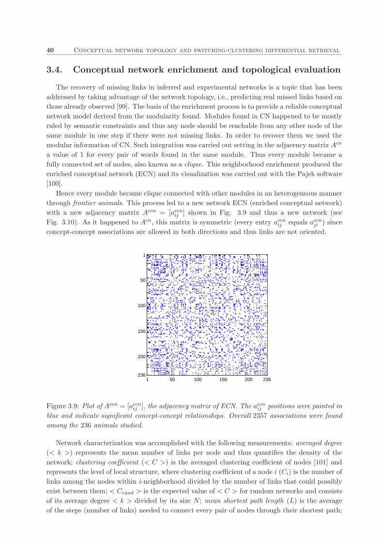
40 Conceptual network topology and switching-clustering differential retrieval
3.4. Conceptual network enrichment and topological evaluation
The recovery of missing links in inferred and experimental networks is a topic that has been
addressed by taking advantage of the network topology, i.e., predicting real missed links based on
those already observed [99]. The basis of the enrichment process is to provide a reliable conceptual
network model derived from the modularity found. Modules found in CN happened to be mostly
ruled by semantic constraints and thus any node should be reachable from any other node of the
same module in one step if there were not missing links. In order to recover them we used the
modular information of CN. Such integration was carried out setting in the adjacency matrix Acn
a value of 1 for every pair of words found in the same module. Thus every module became a
fully connected set of nodes, also known as a clique. This neighborhood enrichment produced the
enriched conceptual network (ECN) and its visualization was carried out with the Pajek software
[100].
Hence every module became clique connected with other modules in an heterogeneous manner
through frontier animals. This process led to a new network ECN (enriched conceptual network)
with a new adjacency matrix Aecn = [aecnij ] shown in Fig. 3.9 and thus a new network (see
Fig. 3.10). As it happened to Acn, this matrix is symmetric (every entry aecnij equals aecn
ji ) since
concept-concept associations are allowed in both directions and thus links are not oriented.
1 50 100 150 200 236
1
50
100
150
200
236
Figure 3.9: Plot of Aecn = [aecnij ], the adjacency matrix of ECN. The aecn
ij positions were painted in
blue and indicate significant concept-concept relationships. Overall 2357 associations were found
among the 236 animals studied.
Network characterization was accomplished with the following measurements: averaged degree
(< k >) represents the mean number of links per node and thus quantifies the density of the
network; clustering coefficient (< C >) is the averaged clustering coefficient of nodes [101] and
represents the level of local structure, where clustering coefficient of a node i (Ci) is the number of
links among the nodes within i-neighborhood divided by the number of links that could possibly
exist between them; < Crand > is the expected value of < C > for random networks and consists
of its average degree < k > divided by its size N ; mean shortest path length (L) is the average
of the steps (number of links) needed to connect every pair of nodes through their shortest path;

Section 3.4 41
beebumblebee
miteeagle
golden eagle
harrier
scorpion2
moose
clam
anchovy
antelope
spider
squirrel
herring
donkey2
tuna
ostrichwasp
cod
whale barbsea bream
bison
boa
European lobster
skipjack tuna
ox
edible crab
buffalo
owlvulture
donkey
sea horse
horse
goat
Goat-kid
cockatoo
sperm whale
alligator
squid
chameleon
camel
canary
crab
kangaroo
snail
caribou
male sheep
carp
rattle snake
zebra
spider crab
pig
common kestrel
jackal
chimpanzeecentipede
deer
Norway lobster
cicada
stork
swan
guinea pig
cobra
crocodile
quail
weasel
condor
rabbit
conger
lamb
cormorantroe deer
coyote
cockroach
crow
little snake
dolphin
hilt-head bream
dromedary
elephant
elephant seal
echidna
hedgehog
beetle
scorpion
starfish
seal
gazelle
hen
cock
prawn
fallow deer
goose
tick
catsparrow hawk
seagullswallow
gorilla
small pig
sparrow
cricket
cheetah
worm
silkworm
falcon
hamster
hyena
hippopotamus
ant
ferret
iguana
wild boar
jaguar
goldfinch
giraffe
kiwi
koala
wall lizardlizard
lobster
king prawn
barn owl
sole
lion
sea lion
leoparddragonfly
hare
lynx
llama
wolfearthworm
true parrot
sea bass
glow-worm
northern pike
macaque
mammut
manatee
praying mantis
butterfly
ladybird
jellyfish
musselhake
grouper
kite
monkey
walrus
fly
mosquito
mouflon
mule
velvet crab
gnu
otter
domestic goose
orangutan
killer whale
platypus
caterpillar
bear
anteater
panda
brown bear
polar bear
oyster
sheep
bird
pigeon
dove
panther
parrot
duckturkey
peacock
pelican
barnacle
partridge
budgerigar
dogEuropean robin
fishswordfish
flatfish
manta ray
hammer fish
magpie2
penguin
louse
piranha
python
chicken
pony colt
porcupine
flea
octopus
puma
bearded vulture
frog
monkfish
rat
mouse
ray fish
chamois
reindeer
rhinoceros
turbot
nightingale
salamander
gecko
salmon
grasshopper
toad
sardine
cuttlefish
snake horsefly
badger
calf
shark
tigermole
bull
turtle
trout
toucan
capercaillie
cow
European green finch
viper
mare
fox
Pajek
Figure 3.10: Enriched conceptual network (ECN). Size of nodes represents its frequency, color
indicates its module belonging and matches with the dendrogram color legend of figure 3.7. Links
stand for concept associations and thus allowed clustering transitions.

42 Conceptual network topology and switching-clustering differential retrieval
Table 3.3: Network analysis. Topological features of the conceptual network (CN) and the enriched
conceptual network (ECN).
Term CN ECN Description
N 236 236 number of nodes (animals)
links 611 2357 number of interactions (concept relationships)
D 9 6 diameter of the network
L 4.40 3.24 mean length of pairwise shortest paths
< k > 5.18 19.97 averaged degree of the network
< C > 0.33 0.87 clustering coefficient of the network
< Crand > 0.021 0.084 < C > for a random network (size N ,< k >)
diameter (D) is the longest among all shortest paths, i.e. the minimum number of links that
separate the two farthest nodes within the network.
The topological features before and after the enrichment (CN and ECN respectively) are shown
in Table 3.3. Enriching the network reduced the diameter from 9 to 6 (i.e. every animal can be
attained from any other animal in no more than six steps along ECN) and the mean shortest path
length from 4.40 to 3.24 (i.e. the shortest path length between every two nodes is on average
shorter in ECN). Both network diameters were quite short due to a small-world phenomena
[101] produced by frontier animals that act as short-cuts i.e. links that connect different regions
(modules in this case) of the network. Example of animals linking two or more modules (frontier-
animals) are monkey and crocodile. Crocodile is part of the reptiles module but has five links
towards sabana, while monkey has three links with sabana but conforms an independent module
with other apes. Finally, the conversion of every module to a clique multiplied by almost four the
averaged degree of the network and increased the clustering coefficient from 0.33 to 0.87. The
expected clustering coefficient in a random network of the same size and average degree would
have been 0.021 and 0.08 for CN and ECN respectively. The difference in one order of magnitude
between < Crand > and < C > for both networks shows the presence of high organization. In
other words, concepts indirectly linked through a common neighbor are more likely to be directly
linked, a phenomena not observed when there is a uniform random linkage of nodes in a network.
Conceptual networks used as in-silico judges of switching and clustering
In order to evaluate ECN as an in-silico judge of clustering and switching transitions, those
animals not represented in the networks were removed from verbal fluency tests. Every transition
was labeled as clustering when both concepts were directly linked on the network and as switching
otherwise. Those 21 out of 200 tests where more than 10% of concepts had been eliminated were
not considered in order to avoid methodological biases. The 179 remaining tests were converted
to binary vectors where switching and clustering transitions were labeled according to CN and
ECN. Every transition was labeled as clustering when both concepts were directly linked on the
network and as switching otherwise. Finally, 20 of these tests were randomly selected and two
experimented judges manually evaluated switching and clustering transitions in order to provide
an inter-rater agreement between human expertise and our unsupervised approach. Inter-rate
agreements between every expert and in silico outputs were measured by kappa coefficient κ
[102]. The equation for κ is:

Section 3.4 43
Table 3.4: Sheet of the variables used to compute κ inter agreement coefficient. N is the to-
tal number of word transitions evaluated; a and c are the number of agreements for switching
and clustering respectively; b and d are the number of disagreements switching-clustering and
clustering-switching respectively.
judge1/judge2 switching clustering total
switching a b r
clustering c d s
total t u N
Table 3.5: Inter-rater agreement. Kappa values among in-silico CN and ECN models and human
expertise of two judges.
rater CN ECN judge 1 judge 2
CN 1 0.85 0.70 0.71
ECN 0.85 1 0.82 0.83
judge 1 0.70 0.82 1 0.88
judge 2 0.71 0.83 0.88 1
κ =P (o) − P (e)
1 − P (e), (3.7)
where P (o) is the relative observed agreement and P (e) is the hypothetical probability of chance
agreement. If the judges are in complete agreement then κ = 1. If there is no agreement among
the judges (other than what would be expected by chance) then κ ≤ 0. Equations for P (o) and
P (e) are
P (o) =a + d
N, P (e) =
rt + su
N2. (3.8)
The meaning of the variables needed are summarized in Table 3.4.
Table 3.5 shows inter-rate agreements among in-silico and human judge expertise. While CN
evaluation is in good concordance with human judgment (0.71 and 0.70), ECN shows a higher
agreement (0.82 and 0.83) very close to the kappa coefficient found between the two judges
(0.88). Hence ECN is a conceptual representation closer to human evaluation than CN and
represents an unsupervised reliable approach. Summarizing ECN is an unsupervised network
model of lexical organization based on the evidences collected from 200 verbal fluency tests after
detecting significant co-occurrences and after enriching the network with the modular semantic
knowledge found. Such model aims to represent conceptual storage structure and its links stand
for word related transitions (clustering) while its disconnected pairs for word unrelated transitions
(switching).
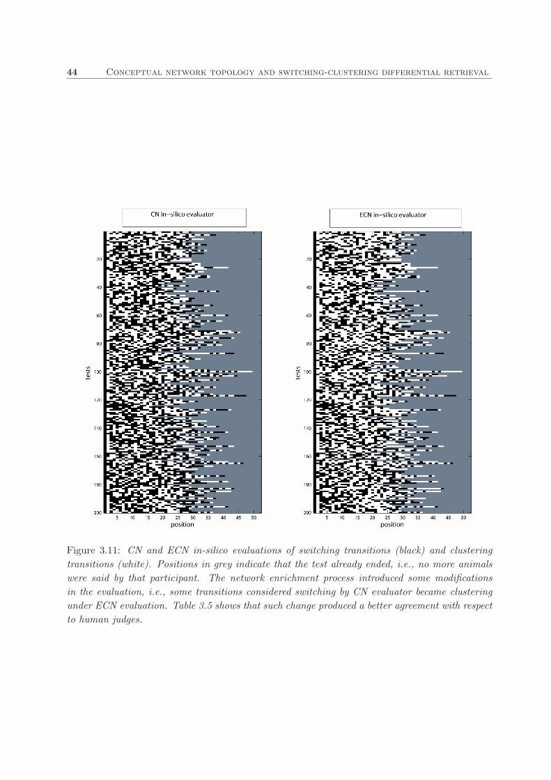
44 Conceptual network topology and switching-clustering differential retrieval
Figure 3.11: CN and ECN in-silico evaluations of switching transitions (black) and clustering
transitions (white). Positions in grey indicate that the test already ended, i.e., no more animals
were said by that participant. The network enrichment process introduced some modifications
in the evaluation, i.e., some transitions considered switching by CN evaluator became clustering
under ECN evaluation. Table 3.5 shows that such change produced a better agreement with respect
to human judges.
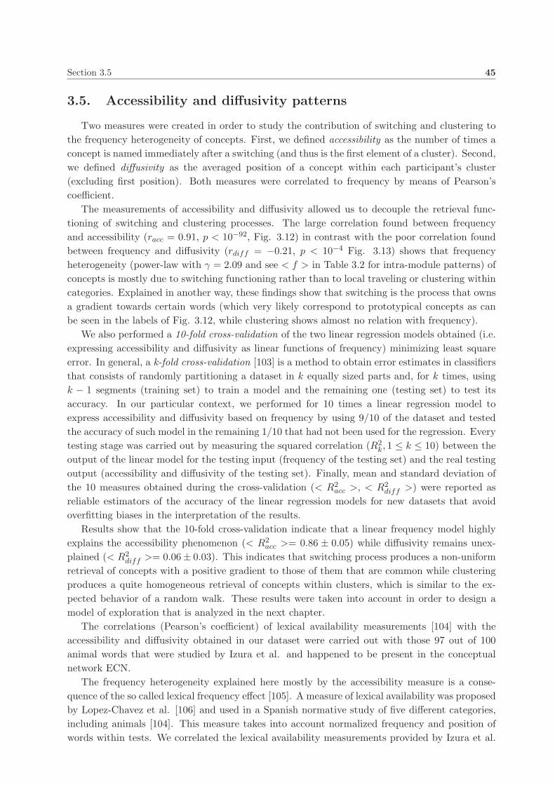
Section 3.5 45
3.5. Accessibility and diffusivity patterns
Two measures were created in order to study the contribution of switching and clustering to
the frequency heterogeneity of concepts. First, we defined accessibility as the number of times a
concept is named immediately after a switching (and thus is the first element of a cluster). Second,
we defined diffusivity as the averaged position of a concept within each participant’s cluster
(excluding first position). Both measures were correlated to frequency by means of Pearson’s
coefficient.
The measurements of accessibility and diffusivity allowed us to decouple the retrieval func-
tioning of switching and clustering processes. The large correlation found between frequency
and accessibility (racc = 0.91, p < 10−92, Fig. 3.12) in contrast with the poor correlation found
between frequency and diffusivity (rdiff = −0.21, p < 10−4 Fig. 3.13) shows that frequency
heterogeneity (power-law with γ = 2.09 and see < f > in Table 3.2 for intra-module patterns) of
concepts is mostly due to switching functioning rather than to local traveling or clustering within
categories. Explained in another way, these findings show that switching is the process that owns
a gradient towards certain words (which very likely correspond to prototypical concepts as can
be seen in the labels of Fig. 3.12, while clustering shows almost no relation with frequency).
We also performed a 10-fold cross-validation of the two linear regression models obtained (i.e.
expressing accessibility and diffusivity as linear functions of frequency) minimizing least square
error. In general, a k-fold cross-validation [103] is a method to obtain error estimates in classifiers
that consists of randomly partitioning a dataset in k equally sized parts and, for k times, using
k − 1 segments (training set) to train a model and the remaining one (testing set) to test its
accuracy. In our particular context, we performed for 10 times a linear regression model to
express accessibility and diffusivity based on frequency by using 9/10 of the dataset and tested
the accuracy of such model in the remaining 1/10 that had not been used for the regression. Every
testing stage was carried out by measuring the squared correlation (R2k, 1 ≤ k ≤ 10) between the
output of the linear model for the testing input (frequency of the testing set) and the real testing
output (accessibility and diffusivity of the testing set). Finally, mean and standard deviation of
the 10 measures obtained during the cross-validation (< R2acc >, < R2
diff >) were reported as
reliable estimators of the accuracy of the linear regression models for new datasets that avoid
overfitting biases in the interpretation of the results.
Results show that the 10-fold cross-validation indicate that a linear frequency model highly
explains the accessibility phenomenon (< R2acc >= 0.86 ± 0.05) while diffusivity remains unex-
plained (< R2diff >= 0.06± 0.03). This indicates that switching process produces a non-uniform
retrieval of concepts with a positive gradient to those of them that are common while clustering
produces a quite homogeneous retrieval of concepts within clusters, which is similar to the ex-
pected behavior of a random walk. These results were taken into account in order to design a
model of exploration that is analyzed in the next chapter.
The correlations (Pearson’s coefficient) of lexical availability measurements [104] with the
accessibility and diffusivity obtained in our dataset were carried out with those 97 out of 100
animal words that were studied by Izura et al. and happened to be present in the conceptual
network ECN.
The frequency heterogeneity explained here mostly by the accessibility measure is a conse-
quence of the so called lexical frequency effect [105]. A measure of lexical availability was proposed
by Lopez-Chavez et al. [106] and used in a Spanish normative study of five different categories,
including animals [104]. This measure takes into account normalized frequency and position of
words within tests. We correlated the lexical availability measurements provided by Izura et al.
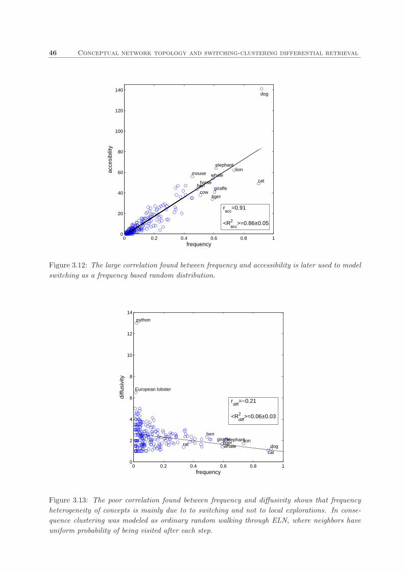
46 Conceptual network topology and switching-clustering differential retrieval
0 0.2 0.4 0.6 0.8 10
20
40
60
80
100
120
140
frequency
acce
sibi
lity
dog
catwhale
elephant
giraffe
lion
tiger
horsehen
cow
mouse
racc
=0.91
<R2acc
>=0.86±0.05
Figure 3.12: The large correlation found between frequency and accessibility is later used to model
switching as a frequency based random distribution.
0 0.2 0.4 0.6 0.8 10
2
4
6
8
10
12
14
frequency
diffu
sivi
ty
python
catdog
lionelephantgiraffe
whaletiger
hen
rat
European lobster
rdiff
=−0.21
<Rdiff2 >=0.06±0.03
Figure 3.13: The poor correlation found between frequency and diffusivity shows that frequency
heterogeneity of concepts is mainly due to to switching and not to local explorations. In conse-
quence clustering was modeled as ordinary random walking through ELN, where neighbors have
uniform probability of being visited after each step.

Section 3.5 47
with accessibility and diffusivity of our dataset giving rise to 0.77 and −0.29 respectively. These
results indicated again, by means of an external validation, the relevant role of switching and the
low role of clustering in the frequency heterogeneity of naming concepts.

48 Conceptual network topology and switching-clustering differential retrieval
3.6. Discussion
In Sections 3.2, 3.3 and 3.4 we respectively inferred a lexical network, extracted its modules
and used them to enrich the network. CN was obtained linking those concepts that co-occurred
significantly. Module extraction was carried out with the GTOM algorithm and showed 16 mod-
ules strongly addressed by semantic features. We integrated modularity results in the network
by converting each module into a clique to create a final network (ECN). This network connects
any two concepts found to be in the same module, and thus semantically related, keeping at the
same time the links between modules trough frontier animals. Finally, in Section 3.5 we assessed
the frequency heterogeneity of concepts in terms of switching and clustering and obtained that
switching is the major responsible of it while clustering poorly contributes to such diversity within
clusters.
A relevant issue addressed in this chapter is the design of an unsupervised novel statistical
methodology which permits to extract co-occurrences above chance from verbal fluency data
taking into account the frequency of each word, a window length, the number of participants and
the mean length of the tests. The major advantage of an unsupervised approach is that concept
relationships do not depend on expert judgment but only on empirical evidences and allowed a
reliable in-silico evaluation of switching and clustering. When compared to previous works of
semantic distance [61, 87–90], it does not need concepts to be named by a large proportion of
participants, which maximizes the number of final elements taking part in the model. Similarly
the use of GTOM led to the finding of modules that when analyzed showed semantic features.
This methodology could be used in the future to explore different domains of semantic memory or
to create syntactic networks from linguistic corpora adding a confidence interval to methodologies
already used [46]. In particular CN is a powerful tool to go in depth into the complex structure
of semantic organization while ECN could be used as a unsupervised tool for quantifying the
clustering and switching phenomena in the neuropsychological analysis of verbal fluency tests. It
could also be easily generalized to detect co-occurrence phenomena in other dichotomic data such
as lesion patterns in neuroimaging studies.
Most accepted theories on semantic representation and natural categories consider that cog-
nitive categories do not have clear-cut frontiers. Elements are better or worse examples of their
categories conforming a prototypicality decay from the central concepts [68, 107]. Although a
limitation of a modular partitioning is that a concept only pertains to one module, in our ap-
proach those animals with a fuzzy module belonging still have links towards other modules. We
defined those nodes as frontier animals and crocodile or monkey are clear examples of short-cuts
between modules, as commented in Section 3.4. A careful analysis of GTOM clustering (see Fig.
3.7) shows evidences of certain hierarchical organization of the modularity, with highly connected
submodules nested into bigger ones. This observation might lead to the reconciliation between the
traditional and intuitive view of hierarchical semantic organization and the complex small-world
and modular structure actually observed. A more detailed analysis of functional hierarchical
modularity would require a much greater sample size, and could use recently proposed tools in
the fields of module and hierarchy detection [99].
The high clustering coefficient and modularity structure are a consequence of the high level of
organization of the semantic storage. However it is well known that both topological properties
impose severe restrictions on the navigability or exploration of the network. However, the presence
of frontier animals (acting as short-cuts and bottlenecks) linking different modules produce an
important decrease of the distance between concepts, which is represented by the small diameter
found in ECN. The presence of frontier items and switching seems to keep the system as a

Section 3.6 49
highly organized structure without jeopardizing the efficient navigability of the network [108].
Furthermore, the combination of this topology and this retrieval strategy could be a very good
balance between organized storage and efficient and robust navigability in the retrieval process.
The large correlation found between accessibility and frequency seems to be due to a posi-
tive gradient for prototypical concepts that might be produced as consequence of its cognitive
over-representation. Interestingly, the poor correlation found between diffusivity and frequency
indicates that such gradient is poorly present in local concept retrieval within categories, and thus
is similar to uniform random selection of terms, at least from a frequency-prototypicality perspec-
tive. Those findings were externally validated by using a lexical availability set of measurements
reported in another dataset. Summarizing switching and clustering processes not only differ in
the regions of the brain involved (there are evidences of a fronto-temporal modulation) but also
in the performance of concept retrieval. From a network theory perspective, clustering seems
to be a random-walker with almost no preferences for concepts that is intermittently shifted to
other locations of the network by an extra-topological mechanism, i.e, switching, with a gradient
towards prototypical or overrepresented concepts that ensures a fast retrieval for those concepts
more usually needed.
Future work could uncover new properties of semantic organization and retrieval in human
cognition, by applying similar or other topological analysis tools and studying other semantic
categories on the networks inferred by this method. Furthermore this methodology might be useful
to better understand the evolution of semantic network acquisition and the relation between verbal
fluency skills in neurodegenerative diseases from an unsupervised dual perspective, i.e. storage
architecture degradation and impaired retrieval abilities.

50 Conceptual network topology and switching-clustering differential retrieval
51
Chapter 4
Switcher random walks: a cognitive
inspired strategy for network
exploration
A dual mechanism based on switching and clustering functioning for random exploration of
networks.
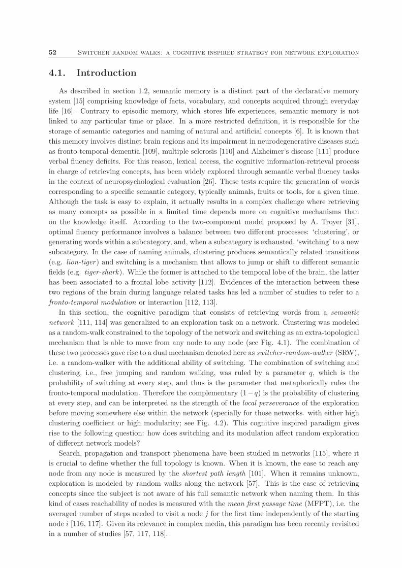
52 Switcher random walks: a cognitive inspired strategy for network exploration
4.1. Introduction
As described in section 1.2, semantic memory is a distinct part of the declarative memory
system [15] comprising knowledge of facts, vocabulary, and concepts acquired through everyday
life [16]. Contrary to episodic memory, which stores life experiences, semantic memory is not
linked to any particular time or place. In a more restricted definition, it is responsible for the
storage of semantic categories and naming of natural and artificial concepts [6]. It is known that
this memory involves distinct brain regions and its impairment in neurodegenerative diseases such
as fronto-temporal dementia [109], multiple sclerosis [110] and Alzheimer’s disease [111] produce
verbal fluency deficits. For this reason, lexical access, the cognitive information-retrieval process
in charge of retrieving concepts, has been widely explored through semantic verbal fluency tasks
in the context of neuropsychological evaluation [26]. These tests require the generation of words
corresponding to a specific semantic category, typically animals, fruits or tools, for a given time.
Although the task is easy to explain, it actually results in a complex challenge where retrieving
as many concepts as possible in a limited time depends more on cognitive mechanisms than
on the knowledge itself. According to the two-component model proposed by A. Troyer [31],
optimal fluency performance involves a balance between two different processes: ‘clustering’, or
generating words within a subcategory, and, when a subcategory is exhausted, ‘switching’ to a new
subcategory. In the case of naming animals, clustering produces semantically related transitions
(e.g. lion-tiger) and switching is a mechanism that allows to jump or shift to different semantic
fields (e.g. tiger-shark). While the former is attached to the temporal lobe of the brain, the latter
has been associated to a frontal lobe activity [112]. Evidences of the interaction between these
two regions of the brain during language related tasks has led a number of studies to refer to a
fronto-temporal modulation or interaction [112, 113].
In this section, the cognitive paradigm that consists of retrieving words from a semantic
network [111, 114] was generalized to an exploration task on a network. Clustering was modeled
as a random-walk constrained to the topology of the network and switching as an extra-topological
mechanism that is able to move from any node to any node (see Fig. 4.1). The combination of
these two processes gave rise to a dual mechanism denoted here as switcher-random-walker (SRW),
i.e. a random-walker with the additional ability of switching. The combination of switching and
clustering, i.e., free jumping and random walking, was ruled by a parameter q, which is the
probability of switching at every step, and thus is the parameter that metaphorically rules the
fronto-temporal modulation. Therefore the complementary (1− q) is the probability of clustering
at every step, and can be interpreted as the strength of the local perseverance of the exploration
before moving somewhere else within the network (specially for those networks. with either high
clustering coefficient or high modularity; see Fig. 4.2). This cognitive inspired paradigm gives
rise to the following question: how does switching and its modulation affect random exploration
of different network models?
Search, propagation and transport phenomena have been studied in networks [115], where it
is crucial to define whether the full topology is known. When it is known, the ease to reach any
node from any node is measured by the shortest path length [101]. When it remains unknown,
exploration is modeled by random walks along the network [57]. This is the case of retrieving
concepts since the subject is not aware of his full semantic network when naming them. In this
kind of cases reachability of nodes is measured with the mean first passage time (MFPT), i.e. the
averaged number of steps needed to visit a node j for the first time independently of the starting
node i [116, 117]. Given its relevance in complex media, this paradigm has been recently revisited
in a number of studies [57, 117, 118].
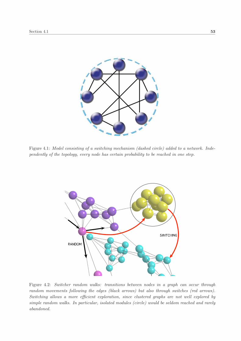
Section 4.1 53
Figure 4.1: Model consisting of a switching mechanism (dashed circle) added to a network. Inde-
pendently of the topology, every node has certain probability to be reached in one step.
Figure 4.2: Switcher random walks: transitions between nodes in a graph can occur through
random movements following the edges (black arrows) but also through switches (red arrows).
Switching allows a more efficient exploration, since clustered graphs are not well explored by
simple random walks. In particular, isolated modules (circle) would be seldom reached and rarely
abandoned.
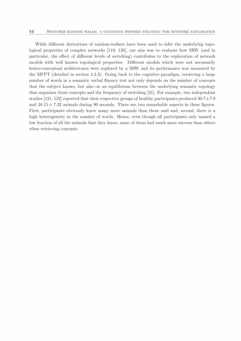
54 Switcher random walks: a cognitive inspired strategy for network exploration
While different derivations of random-walkers have been used to infer the underlying topo-
logical properties of complex networks [119, 120], our aim was to evaluate how SRW (and in
particular, the effect of different levels of switching) contributes to the exploration of network
models with well known topological properties. Different models which were not necessarily
lexico-conceptual architectures were explored by a SRW and its performance was measured by
the MFPT (detailed in section 4.2.3). Going back to the cognitive paradigm, retrieving a large
number of words in a semantic verbal fluency test not only depends on the number of concepts
that the subject knows, but also on an equilibrium between the underlying semantic topology
that organizes those concepts and the frequency of switching [31]. For example, two independent
studies [121, 122] reported that their respective groups of healthy participants produced 30.7±7.9
and 28.15 ± 7.32 animals during 90 seconds. There are two remarkable aspects in these figures.
First, participants obviously knew many more animals than those said and, second, there is a
high heterogeneity in the number of words. Hence, even though all participants only named a
low fraction of all the animals that they know, some of them had much more success than others
when retrieving concepts.
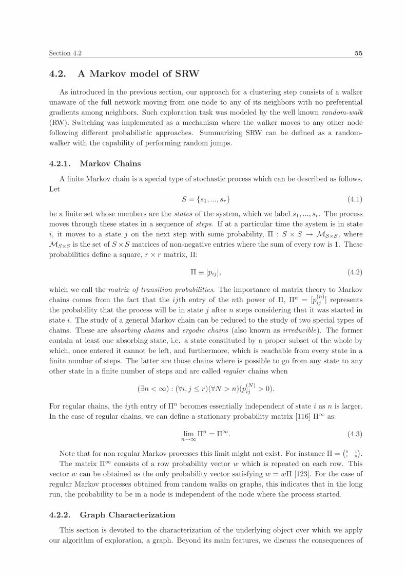
Section 4.2 55
4.2. A Markov model of SRW
As introduced in the previous section, our approach for a clustering step consists of a walker
unaware of the full network moving from one node to any of its neighbors with no preferential
gradients among neighbors. Such exploration task was modeled by the well known random-walk
(RW). Switching was implemented as a mechanism where the walker moves to any other node
following different probabilistic approaches. Summarizing SRW can be defined as a random-
walker with the capability of performing random jumps.
4.2.1. Markov Chains
A finite Markov chain is a special type of stochastic process which can be described as follows.
Let
S = {s1, ..., sr} (4.1)
be a finite set whose members are the states of the system, which we label s1, ..., sr. The process
moves through these states in a sequence of steps. If at a particular time the system is in state
i, it moves to a state j on the next step with some probability, Π : S × S → MS×S , where
MS×S is the set of S×S matrices of non-negative entries where the sum of every row is 1. These
probabilities define a square, r × r matrix, Π:
Π ≡ [pij ], (4.2)
which we call the matrix of transition probabilities. The importance of matrix theory to Markov
chains comes from the fact that the ijth entry of the nth power of Π, Πn = [p(n)ij ] represents
the probability that the process will be in state j after n steps considering that it was started in
state i. The study of a general Markov chain can be reduced to the study of two special types of
chains. These are absorbing chains and ergodic chains (also known as irreducible). The former
contain at least one absorbing state, i.e. a state constituted by a proper subset of the whole by
which, once entered it cannot be left, and furthermore, which is reachable from every state in a
finite number of steps. The latter are those chains where is possible to go from any state to any
other state in a finite number of steps and are called regular chains when
(∃n < ∞) : (∀i, j ≤ r)(∀N > n)(p(N)ij > 0).
For regular chains, the ijth entry of Πn becomes essentially independent of state i as n is larger.
In the case of regular chains, we can define a stationary probability matrix [116] Π∞ as:
limn→∞
Πn = Π∞. (4.3)
Note that for non regular Markov processes this limit might not exist. For instance Π =(
0 1
1 0
)
.
The matrix Π∞ consists of a row probability vector w which is repeated on each row. This
vector w can be obtained as the only probability vector satisfying w = wΠ [123]. For the case of
regular Markov processes obtained from random walks on graphs, this indicates that in the long
run, the probability to be in a node is independent of the node where the process started.
4.2.2. Graph Characterization
This section is devoted to the characterization of the underlying object over which we apply
our algorithm of exploration, a graph. Beyond its main features, we discuss the consequences of
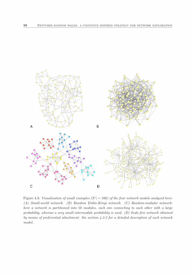
56 Switcher random walks: a cognitive inspired strategy for network exploration
Figure 4.3: Visualization of small examples (|V | = 100) of the four network models analyzed here:
(A) Small-world network. (B) Random Erdos-Renyi network. (C) Random-modular network:
here a network is partitioned into 10 modules, each one connecting to each other with a large
probability, whereas a very small intermodule probability is used. (D) Scale-free network obtained
by means of preferential attachment. See section 4.2.2 for a detailed description of each network
model.

Section 4.2 57
connectedness in order to clearly define the frameworks over which the SRW algorithm can be
defined. Finally, we briefly define the graph models studied numerically in section 4.3.
Let us suppose that our Markov chain is defined by some graph topology. A graph G is defined
by a set of nodes, V ≡ {v1, ..., vn}, and a set of links Γ ≡ {{vi, vj}, ..., {vk, vl}}, being Γ a subset
of V × V . In our approach, the graph is undirected and we avoid the possibility that a node
contains auto-loops or that two links are connecting the same nodes. The size of the graph is |V |,
i.e. the cardinal of the set of vertices. Its average connectivity is defined as:
〈k〉 ≡2|Γ|
|V |. (4.4)
The topology of our graph is completely described by a symmetrical, |V |×|V | matrix, A(G) = [aij ],
the so-called adjacency matrix, whose elements are defined as:
aij =
{
1 ↔ {vi, vj} ∈ Γ
0 otherwise.(4.5)
The connectivity of the node vi, k(vi) is the number of links departing from vi and it can be
easily computed from the adjacency matrix as:
k(vi) =∑
j≤|V |
aij . (4.6)
Following the characterization, we now define the degree distribution, which is understood as the
probability that a randomly chosen node displays a given connectivity. In this way, we define the
elements of such a probability distribution, {p} as:
pi =|(vj ∈ V ) : (k(vj) = i)|
|V |. (4.7)
The above defined measures are the identity card of a given graph G. One could think that
it is enough because our main goal is to describe and characterize an exploration algorithm over
G. However, especially in the models of random graphs, we cannot be directly sure that our
adjacency matrix defines a fully connected graph, i.e, that there exists, with probability 1 a path
from any node vi to any node vj . In deterministic graphs, we can solve this problem by assuming,
a priori, that our combinatorial object is fully connected. Furthermore, we could agree that, when
performing re-wirings at random, we impose the condition of connectedness. The case of pure
random graphs is a bit more complicated. Indeed, a random graph is obtained by a stochastic
process of addition or removal of links [124]. Thus, we need a criteria to ensure that our graph
is connected or, at least, to work over the most representative component of the obtained object.
Full connectedness is hard to ensure in a pure random graph. Instead, what we can find is a
giant connected component, GCC. Informally speaking, we can imagine an algorithm spreading
at random links among a set of predefined nodes, the so-called Erdos-Renyi graph process. The
growing graph displays, at the beginning, a myriad of small clusters of a few nodes and, when
we overcome some threshold in the number of links we spread at random, a component much
bigger than the others emerges, i.e. the GCC [125]. In this way, M. Molloy and B. Reed [126]
demonstrated that, given a random graph with degree distribution {p}, if∑
k
k(k − 2)pk > 0 (4.8)
then, there exists, with high probability, a giant connected component. The first condition we need
to assume is thus, that the studied graphs satisfy inequality defined in equation (4.8). Beyond
this assumption, we impose the following criteria when studying our model networks:

58 Switcher random walks: a cognitive inspired strategy for network exploration
1. In a deterministic graph (for example, a chain or a lattice) where we perform random re-
wirings, we do not allow re-wirings that break the graph.
2. If a graph is the result of a stochastic process, the exploration algorithm is defined only over
the GCC (this could imply the whole set of nodes).
3. The adjacency matrix is the adjacency matrix of the GCC. We remove the nodes that, at
the beginning, participated in the process of construction of G but fell outside the GCC.
All the model graphs studied in this work satisfy the above conditions.
In order to enable useful comparative analysis, we built different networks, all of them with
|V | = 500 nodes and |Γ| = 2000 links. The results were averaged after 100 instances per network
model. Let us briefly define the models studied with our exploration algorithm.
Watts-Strogatz Small-World Network. We built an annulus with 500 nodes in such a
way that every node is connected to 8 different nodes (2000 undirected links) [101]. Once the
annulus was constructed, every link suffered a random re-wiring with connectivity p = 0.05.
Erdos Renyi Graph. Over a set fo 500 nodes we spreaded, at random, 2000 links, avoiding
duplication and self-interaction. It can be shown that the obtained graph displayed a binomial
degree distribution [125]:
pk =
(
|V | − 1
k
)
πk(1 − π)|V |−k−1, (4.9)
being π the probability of two nodes being connected. Its value corresponds to
π = |Γ|
(
|V |
2
)−1
(4.10)
Random-Modular. We built 10 different components of 50 nodes and 200 links, spread at
random (as explained for Erdos Renyi graphs) among the 50 nodes of every component. In this
case, we ensure connectedness of such components. Once the ten components are constructed,
every link suffers a random rewiring with a node either from the same component or not, with
probability p = 0.05.
Preferential Attachment. We provide a seed of 9 connected nodes. Every new node was
connected to 8 of the existing nodes with probability proportional to the connectivity of the
existing nodes, i.e., suppose that, at time t a new node vi comes in to the graph. At this time
step, the graph will display an adjacency matrix A(t).
P(aij(t) = 1) =k(vj)(t − 1)
∑
vk∈Atk(vk)(t − 1)
, (4.11)
where
At = {(vk : ∃l) : (akl(t) > 0)} (4.12)
This operation is repeated in an iterative fashion (i.e., updating A) 8 times per node. It can be
shown that, at the limit of a large number of nodes the outcome of this algorithm generates a
graph whose degree distribution follows a power law [127]:
pk ∝ k−α, (4.13)
with α = 3. It is worth noting that such an algorithm avoids the possibility of unconnected
components.

Section 4.2 59
4.2.3. Random walk over a graph as a Markov Process
In this framework, the transition from node i to j is just the probability that a random-walker
starts from some node i and reaches the node j, after some steps. Consistently, the probability
that being in vi we reach the node vj in a single step (i.e, pij) is:
pij =aij
k(vi)(4.14)
This is the general form for a Markov formalization of a random-walker within a graph defined by
its adjacency matrix A. Throughout this work we assume that our graphs define regular Markov
processes (see section 4.2.1). Under the above definition of Π, regularity is assured if and only if
the graph is not bipartite (i.e., it contains, at least, one loop containing an odd number of nodes).
To see that bipartite graphs are not regular, it is enough to notice that for any pair of nodes
(vi, vj) there are only either odd or even paths joining them, but not both. Hence if p(n)ij 6= 0 then
p(n+1)ij = 0 and therefore the process cannot be regular.
Summarizing, despite that connectedness ensures that the process is ergodic,
(∀vi, vj ∈ G)(∃n : p(n)ij 6= 0)
it does not ensure regularity and therefore the limn→∞ Πn might not exist. The existence of an
odd loop breaks such parity problem and enables Πn to stabilize to a specific matrix of stationary
probabilities when n → ∞. Thus, we must impose another assumption to our studied graphs:
Our algorithm works over non-bipartite graphs which satisfy the criteria imposed in section 4.2.2.
It is straightforward to observe that, if the assumption of regularity holds, the above Markov
process has a stationary state with associated probabilities proportional to the connectivity of
the studied node [57]:
p(∞)ij =
k(vj)
2|Γ|. (4.15)
From now on, we will refer to the transition matrix above defined as Πcl, since it denotes the
probabilities of the movements related to clustering.
4.2.4. Switcher-random-walks
In the retrieval model introduced here, the matrix of transition probabilities Πsrw is a linear
combination of the switching transition probabilities Πsw and the clustering transition probabil-
ities Πcl, as defined in the above section. The Markov process is a switcher-random-walker and
the states represent the location of such walker in the network.
The matrix Πsw = [pswij ] is ergodic and regular since all entries are strictly greater than zero,
and has equal rows, i.e. constant columns. The reason is that the probability of reaching a node
j through switching is independent of the source node i. In this way, we could consider that we
define a scalar field λ over the nodes of the graph:
pswij = λj . (4.16)
Consistently,∑
j≤|V |
λj = 1. (4.17)

60 Switcher random walks: a cognitive inspired strategy for network exploration
We can define this field in many different ways. As the more representative, we revise several
scalar fields that can provide us interesting information about the process:
λj =
1
|V |
k(vj)∑
i≤|V |
k(vi)
K − k(vj) + 1∑
i≤|V |
k(vi)
(4.18)
In the first and most simple case switching to any other node is a random uniform process, and
we refer to this process as uniformly distributed switching. The second case corresponds to the
situation where the probability to reach a given node through switching is proportional to its
connectivity, which we call positive degree gradient switching. The last one assumes that K is
max{k(vi)} and corresponds to the situation where the switcher jumps with more probability to
weakly connected nodes, and we refer to it as negative degree gradient switching. These three
variants of switching were studied when combined with a random-walker within the above graph
topologies (see Fig. 4.4). They were denoted by SRW=, SRW+ and SRW− respectively.
The matrix Πcl = [pclij ] defined in the above section is ergodic and regular but restricted to
the transitions allowed by the adjacency matrix A of the network of study. We modeled as equi-
probable the transitions among linked nodes of the network. Hence the probability of moving
from a node vi to a a node vj through clustering for a given graph G with an adjacency matrix
AG = [aij ], is
pclij =
aij
k(vi). (4.19)
Thus, Πsrw = [psrwij ] is defined as:
Πsrw = qΠsw + (1 − q)Πcl (0 ≤ q ≤ 1), (4.20)
where q is the probability of switching. Consistently, the entries of Πsrw are given by:
psrwij = qpsw
ij + (1 − q)pclij , 0 ≤ q ≤ 1. (4.21)
We observed that Πsrw is also ergodic and regular. This follows from the fact that Πsw has
already all entries strictly greater than zero, and thus Πsrw will have all entries greater than zero
for any q > 0. For the case of q = 0, Πsrw is just Πcl which we assumed to be regular.
Among other interesting descriptive random variables that can be evaluated for regular chains,
the matrix of the mean first passage time (MFPT) is a matrix 〈T 〉 = [〈tij〉], crucial for measuring
the retrieval or exploratory performance of any stochastic strategy; the MFPT needed to go from
a node i to a node j is denoted by 〈tij〉 [57] and represents the time (in step units) required to
reach state j for the first time starting from state i. It is important to note that 〈tij〉 is not
necessarily equal to 〈tji〉, i.e. it might happen that the time required to go from state i to state
j is different to the time required to go from state j to state i.

Section 4.2 61
In order to obtain the analytical expression of MFPT, we must define first a fundamental
matrix Z [123] which is given by
Z = (I − Πsrw + Π∞srw)−1, (4.22)
where
Π∞srw = lim
n→∞(Πsrw)n , (4.23)
and I is the identity matrix of size |V | × |V |.
In this case the entry zij of Z can be understood as a measure of the deviations of the ijth
entry of (Πsrw)n from their limiting probabilities w, which, as commented in section 4.2.1, is any
of the equal rows of Π∞srw. From Z and w we can obtain the analytical derivation of 〈T 〉 = [〈tij〉]
(for more details see Grinstead et al. [123]):
〈tij〉 =zjj − zij
wj(4.24)
Finally, we denote as 〈MFPT 〉G the averaged value of all entries 〈tij〉 for a switcher random
walker exploring a network G. Since 〈T 〉 it is not necessarily symmetrical, we must take into
account all the entries outside the main diagonal. The main diagonal was not taken into account,
since it represents the returning time, which we do not consider as a part of the exploration of
the network. Thus,
〈MFPT 〉G =1
2(
|V |2
)
∑
i
∑
j 6=i
〈tij〉. (4.25)
This measure provides a general evaluation of how reachable is, on average, any node from any
other node in a specific network using a switcher random-walker. It is interesting to notice that
such measure has an upper bound which is precisely the size of the network. Indeed, let us
suppose we have a clique of size m, i.e., a graph, G(V, Γ), where |V | equals m and every node
vi is connected to itself and to all m − 1 remaining nodes. It corresponds to the case where the
probability of switching is 1. Let X be a random variable whose outcomes are vj such that,
∀vj ∈ V :
P(X = vj) =1
m. (4.26)
We define a stochastic process, namely, the realizations of X through different time steps,
X(1), X(2), ..., X(t) Let us define another random variable, Y , namely the number of realiza-
tions of X needed to ensure that there has been one realization of X equal to vj :
Y = mint{X(t) = vj} (4.27)
Clearly, and due to the symmetry of our experiment, all the nodes behave in the same way.
Furthermore,
〈Y 〉 = m (4.28)
i.e., we need, in average m realizations of X in order to obtain, at least, one realization X = vj ,
∀vj ∈ V . We observe that the above random experiment is exactly a random switching over a
graph containing m nodes, and that 〈Y 〉 is the 〈MFPT 〉 of this process. Let us suppose we have
a 〈MFPT 〉 < m. This implies that, in average
(∀vj)P(X = vj) >1
m(4.29)
62 Switcher random walks: a cognitive inspired strategy for network exploration
which is a contradiction, since the graph has m nodes. Thus, for a given graph G(V, Γ):
〈MFPT 〉G ≥ |V |. (4.30)
This value represents an horizontal asymptote in the model of SRW as q increases, and it is clearly
defined in our model experiments (see Fig. 4.4).

Section 4.3 63
4.3. Results & discussion
Our main result was that SRW exploration, a cognitive inspired strategy that combines
random-walks with switching for random exploration of networks, decreased the 〈MFPT 〉 of
all models for all SRW variants. This means that, on average, the number of steps needed to
travel between every pair of nodes decreases and thus the overall exploration abilities of a SRW
within the networks improves respect to RW.
0 0.2 0.4 0.6 0.8 1
500
600
700
800
900
1000
<M
FP
Tne
t>
0 0.2 0.4 0.6 0.8 1 0 0.2 0.4 0.6 0.8 1
scale−free
small−world
random
random−modular
SRW−SRW+
q q q
SRW= CBA
Figure 4.4: Exploration performance based on the 〈MFPT 〉G (see equation 4.25) on 4 graph
models for the three Markovian variants of SRW (see equation 5.2 for implementation details of
each variant of switching). Parameter q stands for probability of switching (see equation 4.20).
(A) SRW=, SRW that contains a uniformly distributed switching. (B) SRW+, SRW that contains
a switching with positive degree gradient. (C) SRW−, SRW that contains a switching with negative
degree gradient.
Regarding SRW= (Fig. 4.4A), exploration performance of random-modular and small-world
networks severely improves, overtaking scale-free at q = 0.1. Moreover, at q = 0.3 all the networks
but scale-free superposed, leading to a remarkable scenario where modularity and high clustering
coefficients are not topological handicaps for an efficient information retrieval.
Switching in SRW+ dramatically improves 〈MFPT 〉 in modular and small-world networks
while hardly decreases it in scale-free and random. The reason is that a random-walker on both
kind of networks already shows a gradient to visit highly connected nodes [57], and a positive-
degree switching supported rather than compensated this effect due to redundancy on hubs (see
Fig. 4.4B).
In SRW−, intermediate values of q (around 0.6 for all but scale-free models) showed optimal
performance with a simillar effect to the one produced by SRW=. However, it only partially
64 Switcher random walks: a cognitive inspired strategy for network exploration
succeeded in compensating the already commented natural RW gradient for hubs. (Fig. 4.4C).
Interestingly, the q values close to 1 produced an inverse situation where hubs are so unlikely to
be reached that the overall exploration performance decreased for all the models but dramatically
for scale-free model, where the degree heterogeneity is specially high. On the contrary, small-
world model showed a very similar performance when explored by any of the three SRW variants.
The reason is that in this model, the degree distribution is very homogeneous, and thus different
degree gradients of switching produced very little differences.
The approximate convergence of the exploration efficiency (for most of the topologies when
using SRW= or SRW− with a moderate switching rate) allows a system to organize information
or to evolve without compromising exploration and retrieval efficiency. In this sense, semantic
memory might be organizing information in a strongly modular or locally clustered way without
compromising retrieval performance of concepts. In a more general perspective, the addition of
a switching mechanism and its interaction with random-walk dynamics opens a new framework
to understand processes related to information storage and retrieval. Indeed, switching not only
mitigates exploration deficits of certain network topologies but also might provide certain robust-
ness to the system. For instance, the rewired links (known as short-cuts) in both small-world and
random-modular models are contributing to facilitate access to different regions of the network.
Those short-cuts might compensate a switching impairment or dysfunction and vice versa, i.e.
switching would ensure an accurate exploration of the network even though a targeted attack
removed those short-cuts permanently.
The model proposed here could have implications in other systems that usually have a conflict
between organization and retrieval efficiency. It will be object of further studies in other phe-
nomena unrelated to cognitive processes such as infection epidemiology, information spreading or
energy landscapes.
65
Chapter 5
Switcher Random Walks on the
conceptual network ECN
A model of semantic memory exploration and retrieval during semantic verbal fluency tasks.

66 Switcher Random Walks on the conceptual network ECN
5.1. Cognitive background and motivation
During the verbal fluency experiment, we found a high heterogeneity in the word frequencies,
i.e., a few animals were named by many participants while other animals were named only by a
few participants. We also noticed that the averaged position for a given word within the verbal
fluency tests depended strongly on the above mentioned frequency. These findings were described
in detail in chapter 2. This dependency is a consecuence of the retrieval strategy.
A. Troyer proposed in [31] a strategy consisting of consecutively producing related words until
a category is exhausted and then switching to a new category. With Troyer’s idea in mind, we
built an unsupervised model of conceptual organization, obtaining a network that we called ECN
(see section 3.4 for details). This network allowed us to distinguish the two kind of transitions
between concepts (switching and clustering) that occur in the verbal fluency tests. That is,
if two consecutive concepts within a test were linked in ECN, we had an instance of clustering.
Otherwise we had an instance of switching. We also showed how this strategy combining switching
and clustering produces frequency heterogeneity and averaged position dependence on frequency.
These findings were later considered in chapter 4 to build a model of exploration and retrieval
(SRW) for a number of network models.
In the present chapter, we analyze how exploration based on SRW performs in the case of the
conceptual network obtained from our data (ECN). Such performance was measured for different
degrees of switching, using the averaged mean first passage time 〈MFPT 〉ecn as described in
section 4.2.3.
Previous models of semantic memory retrieval that take into account the dynamics found in
verbal fluency tests have been reported in the literature; for a review see Wixted, 1994 [30]. For
instance, a simple model based on random recovery of elements is able to explain the decay in the
number of concepts named along time [27, 128]. In these models such decrease is explained by
the fact that randomly searched elements can be chosen more than once, and thus increasingly
delay the utterance of unsaid concepts. However this model cannot explain the temporal interval
between words found in fluency and memory tasks. Three major findings have been reported in
these studies: Firstly, time increased as a function of output position within a cluster (e.g., the
time between the first two words was less than between the second and the third); Secondly, time
decreased as a function of cluster size at a given output position (e.g., the period between the two
initial words of a three word cluster was longer than in a five word cluster); Thirdly, time between
the last two words of a cluster was always the same independently of its size [129]. Two-stage
models have been used to explain these phenomena. In the first step a subcategory is searched
while in the second step items from this subcategory are randomly extracted [28, 129, 130].
Section 5.2 67
5.2. Two variants of switcher random walkers
The results of accessibility and diffusivity obtained in chapter 3 explained the contribution of
switching and clustering to the frequency heterogeneity of concepts. We used here this information
to develop two SRW variants.
As described in section 3.5, the large correlation found between frequency and accessibility
(r = 0.91, Fig 3.4) in contrast with the poor correlation found between frequency and diffusivity
(r = −0.21, Fig. 3.5) shows that frequency heterogeneity of words is mostly due to switching
rather than to local traveling or clustering. Explained in another way, these findings show that
switching is the process that drives the system towards frequent words (which correspond to
prototypical concepts), while clustering shows almost no preference (only 4% of the total variance
would be explained by a linear regression model). Those findings based on empirical data were
considered for creating a new variant SRW freq, where the switching random distribution became
frequency dependent. We kept SRW=, described in section 4.2.4, as a baseline naive model.
Hence, as explained in section 4.2.4, we define a scalar field λ over the nodes of the graph:
pswij = λj with
∑
j≤|V |
λj = 1. (5.1)
Such field was defined in two different ways:
λj =
1
|V |
Pwj
n∑
i=1
Pwi
(5.2)
where Pwiis the frequency of word wi divided by the number of tests (see equation (3.1) for
details). In the first and most simple case switching to any other node is a random uniform
process, and we refer to this process as uniformly distributed switching. The second case was
designed according to the results obtained in section 3.5 and corresponds to the situation where
the probability to reach a given node through switching is proportional to its frequency within
the tests, which we call frequency degree gradient switching. Both variants included a random
walker restricted to the network as clustering mechanism (see equation (4.19) for details) and
were denoted by SRW= and SRW freq respectively.
Summarizing, two SRW variants were used in this section. In the original and most naive SRW
(SRW=) clustering was implemented as a random walk within the network (i.e. transition with
equal probability to adjacent nodes) and switching as an extra-topological event not influenced by
neither network structure nor frequency that allows random uniform jumping to any node. A new
variant of the model was also introduced to fit the large frequency-accesibility correlation found.
In this variant, SRW freq, switching was accomplished according to the normalized frequencies
of concepts, instead of being uniformly random distributed. For instance, dog, being the most
named concept, was then the most probable hit of switching. Although clustering/switching ratios
around 0.48 have been reported [31] we evaluated the effect of switching for the full probability
(q) range between 0 (absence of switching) and 1 (absence of clustering).
Both switching variants produced a switching Markov process Πsw = [pswij ] with all entries
greater than zero and thus ergodic and regular. The clustering Markov process Πcl based on the

68 Switcher Random Walks on the conceptual network ECN
adjacency matrix of ECN was also ergodic and regular. The reason is that ECN is connected and
hence ergodic and contains cliques. This implies the presence of odd loops, a property which in
turn ensures regularity (see section 4.2.3 for details). The fact that the transition matrices of both
Markov processes are ergodic and regular is precisely what allows us to calculate the exact values
of 〈tij〉 and thus of 〈MFPT 〉ecn. Hence, we evaluated the exploration performance of SRW= and
SRW freq on the conceptual network ECN as
〈MFPT 〉ecn =1
2(
|V |2
)
∑
i
∑
j 6=i
〈tij〉, (5.3)
where |V | is, in this case, the number of nodes of ECN (236) and 〈tij〉 is the mean first passage
time (i.e. averaged number of steps) to move from a node i to a node j within ECN (see equation
(4.24) for its general definition).
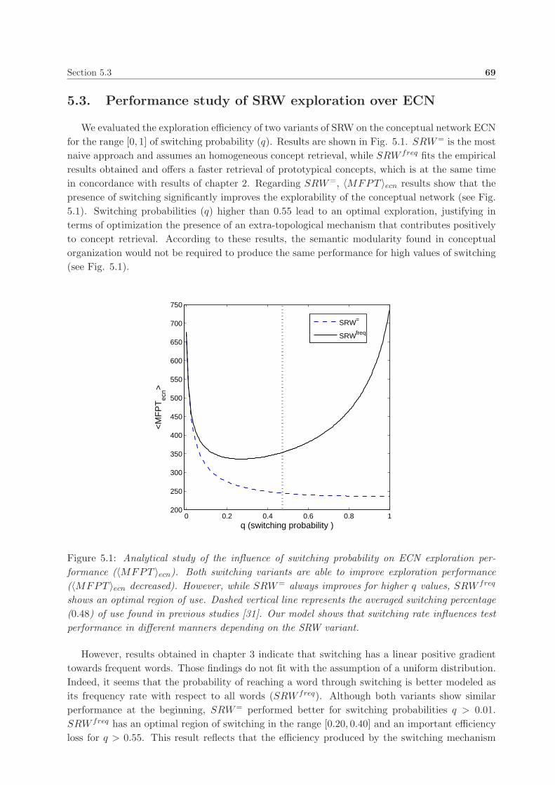
Section 5.3 69
5.3. Performance study of SRW exploration over ECN
We evaluated the exploration efficiency of two variants of SRW on the conceptual network ECN
for the range [0, 1] of switching probability (q). Results are shown in Fig. 5.1. SRW= is the most
naive approach and assumes an homogeneous concept retrieval, while SRW freq fits the empirical
results obtained and offers a faster retrieval of prototypical concepts, which is at the same time
in concordance with results of chapter 2. Regarding SRW=, 〈MFPT 〉ecn results show that the
presence of switching significantly improves the explorability of the conceptual network (see Fig.
5.1). Switching probabilities (q) higher than 0.55 lead to an optimal exploration, justifying in
terms of optimization the presence of an extra-topological mechanism that contributes positively
to concept retrieval. According to these results, the semantic modularity found in conceptual
organization would not be required to produce the same performance for high values of switching
(see Fig. 5.1).
0 0.2 0.4 0.6 0.8 1200
250
300
350
400
450
500
550
600
650
700
750
q (switching probability )
<M
FP
Tec
n>
SRW=
SRWfreq
Figure 5.1: Analytical study of the influence of switching probability on ECN exploration per-
formance (〈MFPT 〉ecn). Both switching variants are able to improve exploration performance
(〈MFPT 〉ecn decreased). However, while SRW= always improves for higher q values, SRW freq
shows an optimal region of use. Dashed vertical line represents the averaged switching percentage
(0.48) of use found in previous studies [31]. Our model shows that switching rate influences test
performance in different manners depending on the SRW variant.
However, results obtained in chapter 3 indicate that switching has a linear positive gradient
towards frequent words. Those findings do not fit with the assumption of a uniform distribution.
Indeed, it seems that the probability of reaching a word through switching is better modeled as
its frequency rate with respect to all words (SRW freq). Although both variants show similar
performance at the beginning, SRW= performed better for switching probabilities q > 0.01.
SRW freq has an optimal region of switching in the range [0.20, 0.40] and an important efficiency
loss for q > 0.55. This result reflects that the efficiency produced by the switching mechanism

70 Switcher Random Walks on the conceptual network ECN
depends drastically on how much it is used when retrieving concepts. Under SRW freq, which
is the model that better integrates retrieval functioning evidences, switching happened to be
especially optimal only for an intermediate region. This result seems to be in agreement with the
obvious difficulty of naming unrelated animals consecutively or naming animals only of the same
semantic category and succeeding on naming plenty of them.
The basis of both variants of the model of semantic memory exploration and retrieval analyzed
here can be explained with a metaphor of a blind bowman, as seen in Fig. 5.2. Let us represent a
bowman located in the frontal lobe shooting his arrows towards the semantic core (switching) in
the temporal lobe which is represented as a modular network of connected concepts. Whenever an
arrow reaches a node in the network a local search process, i.e. clustering, is initiated from it. The
blindness stands for the lack of intentional targets since information retrieval in verbal fluency
task is not deterministic, and thus random shooting. Hence, the distribution of hits depends
only on the representation degree of concepts (size of nodes in our metaphor). Switching follows
a uniform random distribution when nodes are simplified to be equally represented, meanwhile
it follows a frequency dependent distribution when the large correlation between frequency and
accessibility is taken into account. The former assumption was included in SRW= and the latter
in SRW freq, where switching shows an unintentional gradient towards most frequent words that
can be explained by an over-representation or ease of activation of some nodes depending on
its prototypicality. Given the poor correlation found between frequency and diffusivity, both
variants considered clustering as a random walk through the network. Such preferential gradient
is represented in 5.2 by different sized targets.
Although nodes of the same module conform semantic cliques, modules are in general poorly
interconnected with links between frontier animals. The low presence of these links are bottlenecks
that obstruct the traveling of the random walker from one module to another. It is intuitive
to think that high organization of concepts eases semantic processing; however highly modular
networks seriously hindered exploration and thus retrieval of concepts. It seems that the frequent
use of switching is a cognitive dynamical solution for such semantic bottlenecks. Summarizing,
our results with the category of animals show that the human brain seems to have achieved
an optimal balance between high organization based on semantic modularity in the conceptual
structure and high retrieval performance by means of an additional switching mechanism. Finally
it can be hypothesized that frontier animal links and switching are two phenomenon (the former
intrinsic to the topology and the latter extra-topological) with similar function and thus make the
overall system robust. For instance, frontier animals will still allow exploring different semantic
categories if switching fails (frontal damage), and switching might prevent or mitigate retrieval
failures if part of the network become disconnected (temporal damage).

Section 5.3 71
Figure 5.2: A blind bowman; metaphor of the switcher random walker model. Switching, a process
that occurs in the frontal lobe by the executive domain, is modeled as a blind bowman that aims
towards the semantic network in the temporal lobe. His arrows, as he is blind, reach the nodes
of the network only depending in the over-representation of its concepts, represented in the figure
by the size of the nodes. Once such arrow activates a node it begins a random walk that leads to
the enumeration of elements conforming a semantic cluster. In this toy example the exploration
has begun in tiger, one of the most prototypical animal in the sabana module, continuing trough
lion and elephant, going back to tiger, which this time is not overtly said, and finally reaching
hyena. The frontal lobe then initiates a new local search in the reptiles module from snake, passing
through viper and reaching zebra, a sabana animal, through crocodile, which is a frontier animal
between both modules.

72 Switcher Random Walks on the conceptual network ECN

73
Chapter 6
An ontogenic model of the
conceptual network ECN
A topological study of the evolution of the conceptual network of animals by means of concept
frequency as an inverse estimator of its ranked age of acquisition.
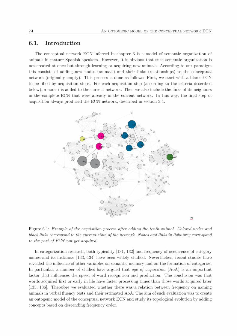
74 An ontogenic model of the conceptual network ECN
6.1. Introduction
The conceptual network ECN inferred in chapter 3 is a model of semantic organization of
animals in mature Spanish speakers. However, it is obvious that such semantic organization is
not created at once but through learning or acquiring new animals. According to our paradigm
this consists of adding new nodes (animals) and their links (relationships) to the conceptual
network (originally empty). This process is done as follows: First, we start with a blank ECN
to be filled by acquisition steps. For each acquisition step (according to the criteria described
below), a node i is added to the current network. Then we also include the links of its neighbors
in the complete ECN that were already in the current network. In this way, the final step of
acquisition always produced the ECN network, described in section 3.4.
whale
horseelephant
hen
cat
giraffe
lion
dog
tiger
cow
Pajek
Figure 6.1: Example of the acquisition process after adding the tenth animal. Colored nodes and
black links correspond to the current state of the network. Nodes and links in light grey correspond
to the part of ECN not yet acquired.
In categorization research, both typicality [131, 132] and frequency of occurrence of category
names and its instances [133, 134] have been widely studied. Nevertheless, recent studies have
revealed the influence of other variables on semantic memory and on the formation of categories.
In particular, a number of studies have argued that age of acquisition (AoA) is an important
factor that influences the speed of word recognition and production. The conclusion was that
words acquired first or early in life have faster processing times than those words acquired later
[135, 136]. Therefore we evaluated whether there was a relation between frequency on naming
animals in verbal fluency tests and their estimated AoA. The aim of such evaluation was to create
an ontogenic model of the conceptual network ECN and study its topological evolution by adding
concepts based on descending frequency order.

Section 6.2 75
6.2. Frequency in verbal fluency: an estimator of ranked age of
acquisition
In this section, we evaluated the use of frequency in verbal fluency for estimating the acquisition
order of animals. The reason is that, as described below, available AoA studies did not cover
even 50% of the elements of the conceptual network ECN, and thus were not enough to produce
its ontogenic model.
The dataset containing 200 verbal fluency tests described in section 2.1 was used here to get
the frequency of each animal, i.e., the number of participants that named each of the 399 different
concepts.
In the last decade,a number of studies regarding age of acquisition of words in Spanish popula-
tion have been published [104, 137, 138]. Cuetos et al. [137] reported an AoA study including 27
animals, Izura et al. [104] included 100 animals and Alvarez et al. [138] included 54 animals. Ad-
ditionally, we averaged the three AoA estimators in a fourth one denoted by 〈AoA〉. Correlations
of these AoA estimators and frequency in our verbal fluency dataset were done with Spearman’s
rank correlation coefficient by using each time the words in common found between every pair of
datasets compared. The reason to use Spearman’s rank correlation instead of Pearson’s correla-
tion coefficient is that the aim of this study was to check whether frequency (sorted from larger
to smaller) produced an accurate ranking of words according to AoA studies rather than testing
whether frequency is linearly correlated to those AoA studies. Results of such correlations can be
seen in Table 6.1 and demonstrate that frequency is negatively correlated with every single AoA
study and indeed is highly correlated to their averaged < AoA > (ρ = −0.63, p < 10−3). Hence,
frequency of concepts in verbal fluency (90 seconds) happened to be an accurate ranking criteria
for ordering concepts according to their AoA.
Table 6.1: Pairwise correlation between AoA estimators previously published and frequency of
animals in our verbal fluency experiment. Detailed tables including every concept, their AoA
according to the studies and their frequency in verbal fluency can be seen in Appendix C
Datasets AoACuetos AoAIzura AoAAlvarez 〈AoA〉 Frequency
AoACuetos - ρ = 0.76, p < 10−4 ρ = 0.73, p < 10−4 - ρ = −0.58, p < 10−2
AoAIzura - - ρ = 0.30, p = 0.04 - ρ = −0.44, p < 10−5
AoAAlvarez - - - - ρ = −0.52, p < 10−4
< AoA > - - - - ρ = −0.63, p < 10−3
Frequency - - - - -

76 An ontogenic model of the conceptual network ECN
3 3.5 4 4.5 5 5.5 6 6.5 7 7.50.1
0.2
0.3
0.4
0.5
0.6
0.7
0.8
0.9
1
spidersquirrel
horse
kangaroo
pig
rabbit
elephant
seal
hen
cat
giraffe
lion
butterfly
monkey
bearsheep
duck
dog
fishfrog
rhinoceros
tiger
cow
fox
<AoA> (years)
freq
uenc
y in
ver
bal f
luen
cy
ρ−spearman = −0.63p < 10 −3
Figure 6.2: Correlation between 〈AoA〉 (years) and frequency (normalized) in our verbal fluency
dataset. Results indicate that the concepts learnt earlier are more frequently named in verbal
fluency.
6.3. Topological measurements
The giant connected component (GCC) of a network, also used in section 4.2.2 refers to the
largest connected subnetwork, i.e., the connected subnetwork that contains a majority of the
entire network nodes. This topological concept was also used in chapter 6. ECN is a connected
giant component itself since it is a connected network. However, this is not necessarily the case
while ECN is being acquired concept by concept.
The topological measurements explained below were applied to the GCC of the ECN ontogeny
model at each step, i.e., every time a concept was added to the network and their links to already
acquired concepts were included. The addition of nodes were done in 2 different ways. First, we
added nodes in a decreasing order of frequency (freqAddition) as an accurate model of conceptual
ontogeny . Second, we added nodes at random (randAddition) to observe the dynamical evolution
of the topological parameters expected by chance .
The randAddition simulations were done 500 times by setting 500 random uniform lists of
concept acquisition. In freqAddition modality, those cases of concepts with equal frequency
were also randomly reshuffled 500 times. Hence both kinds of simulations included an error bar
illustrating the standard deviation of each topological measurement at each step of acquisition.
The clustering coefficient of a system [101], denoted by < C >, is a metric that represents the
density of triangles in a network with n nodes and is measured by
< C >=1
n
n∑
i=1
Ci, (6.1)
where Ci is the clustering coefficient of a node i. For undirected graphs, as the semantic network
Section 6.3 77
studied here, it is measured by
Ci =2|Ni|
(ki − 1)k, 1 ≤ i ≤ n (6.2)
and represents the proportion of links between the set of nodes that are neighbors of node i and
the number of links that could possibly exist between them. Although a modular network will
necessarily have a high clustering coefficient, the opposite statement is not necessarily true. The
reason is that < C > is not strictly a modularity measure. However, we already knew that ECN
is modular (see sections 3.3 and 3.4 for details). Measuring < C > reported us how the clustering
level of the network behaved with the addition of nodes (acquisition of concepts).
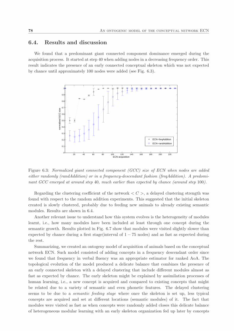
78 An ontogenic model of the conceptual network ECN
6.4. Results and discussion
We found that a predominant giant connected component dominance emerged during the
acquisition process. It started at step 40 when adding nodes in a decreasing frequency order. This
result indicates the presence of an early connected conceptual skeleton which was not expected
by chance until approximately 100 nodes were added (see Fig. 6.3).
20 40 60 80 100 120 140 160 180 200 2200
0.1
0.2
0.3
0.4
0.5
0.6
0.7
0.8
0.9
1
ECN acquisition
norm
aliz
ed G
CC
siz
e
ECN−freqAddition
ECN−randAddition
Figure 6.3: Normalized giant connected component (GCC) size of ECN when nodes are added
either randomly (randAddition) or in a frequency-descendant fashion (freqAddition). A predomi-
nant GCC emerged at around step 40, much earlier than expected by chance (around step 100).
Regarding the clustering coefficient of the network < C >, a delayed clustering strength was
found with respect to the random addition experiments. This suggested that the initial skeleton
created is slowly clustered, probably due to feeding new animals to already existing semantic
modules. Results are shown in 6.4.
Another relevant issue to understand how this system evolves is the heterogeneity of modules
learnt, i.e., how many modules have been included at least through one concept during the
semantic growth. Results plotted in Fig. 6.7 show that modules were visited slightly slower than
expected by chance during a first stage(interval of 1 − 75 nodes) and as fast as expected during
the rest.
Summarizing, we created an ontogeny model of acquisition of animals based on the conceptual
network ECN. Such model consisted of adding concepts in a frequency descendant order since
we found that frequency in verbal fluency was an appropriate estimator for ranked AoA. The
topological evolution of the model produced a delicate balance that combines the presence of
an early connected skeleton with a delayed clustering that include different modules almost as
fast as expected by chance. The early skeleton might be explained by assimilation processes of
human learning, i.e., a new concept is acquired and compared to existing concepts that might
be related due to a variety of semantic and even phonetic features. The delayed clustering
seems to be due to a semantic feeding stage where once the skeleton is set up, less typical
concepts are acquired and set at different locations (semantic modules) of it. The fact that
modules were visited as fast as when concepts were randomly added closes this delicate balance
of heterogeneous modular learning with an early skeleton organization fed up later by concepts

Section 6.4 79
20 40 60 80 100 120 140 160 180 200 2200
0.2
0.4
0.6
0.8
1
ECN acquisition
GC
C −
Clu
ster
ing
coef
ficie
nt
ECN−freqAddition
ECN−randAddition
Figure 6.4: Clustering coefficient evolution of ECN when nodes are added either randomly or in
a frequency-descendant fashion. Clustering coefficient is smaller than expected by chance for a
large intermediate range.
20 40 60 80 100 120 140 160 180 200 220−0.2
0
0.2
0.4
0.6
0.8
1
1.2
1.4
1.6
1.8
ECN acquisition
ratio
inte
r/in
tra
links
freqAddition
randAddition
Figure 6.5: Ratio between links connecting different modules and links within modules. These
ratio is higher than expected by chance for almost all the growing steps. This indicates that links
connecting modules happened very early (giving rise to a heterogeneous conceptual skeleton) while
links internally connecting modules were produced later.
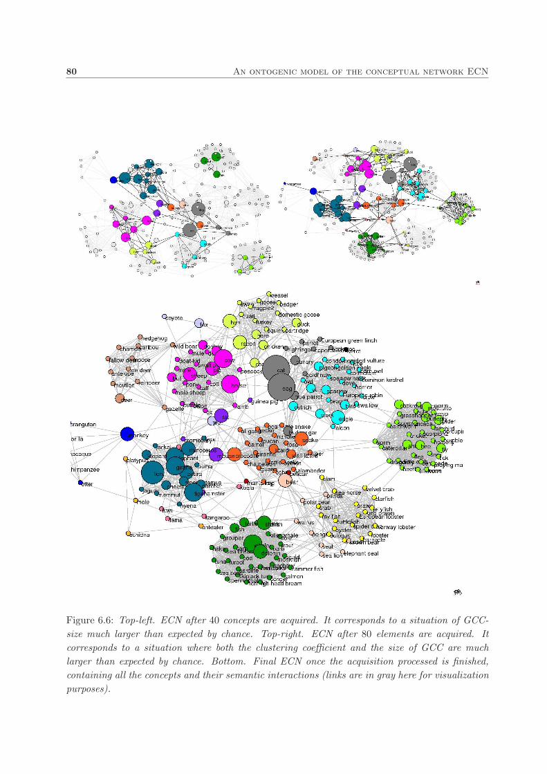
80 An ontogenic model of the conceptual network ECN
Figure 6.6: Top-left. ECN after 40 concepts are acquired. It corresponds to a situation of GCC-
size much larger than expected by chance. Top-right. ECN after 80 elements are acquired. It
corresponds to a situation where both the clustering coefficient and the size of GCC are much
larger than expected by chance. Bottom. Final ECN once the acquisition processed is finished,
containing all the concepts and their semantic interactions (links are in gray here for visualization
purposes).
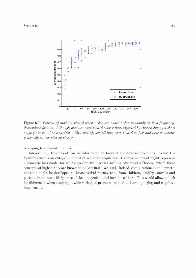
Section 6.4 81
20 40 60 80 100 120 140 160 180 200 2200
0.1
0.2
0.3
0.4
0.5
0.6
0.7
0.8
0.9
1
ECN acquitision
% m
odul
es p
rese
nt
freqAddition
randAddition
Figure 6.7: Percent of modules visited when nodes are added either randomly or in a frequency-
descendant fashion. Although modules were visited slower than expected by chance during a short
stage (interval of adding 40th − 65th nodes), overall they were visited as fast and thus as hetero-
geneously as expected by chance.
belonging to different modules.
Interestingly, this model can be interpreted in forward and reverse directions. While the
forward sense is an ontogenic model of semantic acquisition, the reverse model might represent
a semantic loss model for neurodegenerative diseases such as Alzheimer’s Disease, where those
concepts of higher AoA are known to be lost first [139, 140]. Indeed, computational and heuristic
methods might be developed to locate verbal fluency tests from children, healthy controls and
patients in the most likely state of the ontogenic model introduced here. This would allow to look
for differences when studying a wide variety of processes related to learning, aging and cognitive
impairment.
82 An ontogenic model of the conceptual network ECN

83
Chapter 7
Lexical access impairment in
neurodegenerative conditions
A contribution towards the understanding of different issues that affect lexical access and
retrieval in neurodegenerative diseases.
84 Lexical access impairment in neurodegenerative conditions
7.1. Multiple sclerosis
Multiple Sclerosis (MS) is a chronic inflammatory and neurodegenerative disease of the central
nervous system [141]. It has been generally considered a disease of the white matter. However,
this is only one pathological aspect of the disease as demyelination is prominent in the grey
matter of deep cerebral nuclei and the cerebral cortex and thus the disease involvement of grey
matter structures may significantly contribute to clinical disability in multiple sclerosis patients
[142]. Indeed, while lesions involving the white matter (WM) are well known, recent studies
have also indicated extensive damage of the grey matter (GM), including microglia activation,
cortical demyelization, and axonal, synaptic, and neuronal loss [142–146]. Recently, the extension
and pathological basis of GM pathology have been highlighted by means of pathological and
neuroimaging studies [147]. GM atrophy begins early and evolves over the course of the disease.
Volume of GM tissue is lower in MS patients than in control subjects [148–150]. The study of
GM damage is of critical importance since axonal and neuronal damage are the main factors
responsible for long-term disability in MS [151].
Cognitive impairment is frequent in patients with Multiple Sclerosis (MS), significantly re-
ducing their quality of life. Language is one of the domains affected in MS but its involvement
is not well understood. Despite the growing awareness of different cognitive changes in Multi-
ple Sclerosis (MS), high level language functions and communication abilities in these patients
remain poorly understood. Cognitive disturbances are frequent in MS approximately involving
45− 65% of the patients [121, 152–154]. The cognitive functions or domains most often impaired
reported are memory (in different modalities), information processing speed, attention, executive
functions and verbal fluency [154–157]. In particular, declarative verbal memory is one of the
domains that more deteriorates with disease progression. However, it has been claimed that high
level language-related abilities are not significantly impaired in MS, and few attempts have been
done to unveil these alterations.
Semantic and phonemic verbal fluency tests have been used as a language-related task in MS,
showing a consistent decrease of the total number of generated words [110, 154]. Furthermore,
this measure of verbal fluency has been proposed as one of the most sensitive markers of cognitive
impairment in MS derived from the data of a meta-analysis [110]. A possible explanation for
such verbal fluency decrease, supported by previous data [34], is that these patients more than
suffering a degradation of the existing lexical pool fail in the retrieval of lexical information.
However, few steps have been done to analyze this specific lexical access problem in MS. In this
sense, it could be hypothesized that patients suffer an alteration in lexical access involving a
specific impairment in the lexical selection process due to white matter disrupted connections
between cortical areas (mainly temporo-frontal connections) rather than an alteration in the
storage system. This preferential involvement of lexical retrieval could be due to its dependence
of long white matter tracts, which are more frequently damaged in MS.
Neuroimaging studies have identified abnormalities in the GM of patients with MS, mainly
volumetric changes. There are different approaches for detecting and quantifying the subtle
neuropathological alterations taking place in the brain tissue in MS patients , including the
magnetization transfer ratio, diffusion-weighted imaging, or magnetic-resonance spectroscopy.
Recently, we found that fractal dimension (FD) identifies changes in the WM [158] and the GM
[151] of MS patients, including the normal-appearing WM, even at the early stage of the disease.
FD is a measurement of the geometrical complexity of an object, and thus changes in the FD
indicate alterations in the tissue structure under study. Because the WM has a highly complex
anatomy such as the presence of axonal bundles, a pathological process that destroys brain tissue
Section 7.1 85
by creating an amorphous glial scar would decrease the FD of this tissue, as was the case of WM
in MS. Thus, FD might be used as a marker of the degree of brain damage.
86 Lexical access impairment in neurodegenerative conditions
7.2. Mild cognitive impairment
Mild cognitive impairment (MCI) is a concept evoked to fill the diagnostic gap between benign
age-associated forgetfulness and dementia, particularly Alzheimer’s disease.
Different definitions of MCI and closely related terms have been proposed (for review, see [159–
162]. They differ in three ways: firstly on whether formal cognitive testing is required for the
diagnosis; secondly on the distributional criterion for impairment (e.g. certain standard deviation
units below the mean); thirdly on which abilities are to be impaired. MCI may thus include
amnesic MCI with isolated memory impairment, multi-domain MCI with memory and additional
cognitive impairment, and non-amnestic MCI with intact memory but impairment in some other
cognitive ability [143]. Other data-driven subdivisions of MCI might emerge depending on the
aim and direction of the test battery used, on the nature of the sample, and on the statistical
procedures used to arrive at a classification of patients into subgroups. One aim in identifying
subdivisions of MCI is to identify patterns that predict different forms of dementia on longitudinal
studies [163].
Impaired declarative memory acquisition is considered the hallmark of MCI [161]. This may be
documented by tests of delayed recall such as the Auditory-Verbal Learning Test of Rey (1964).
However, there is also evidence for impairments on MCI that go beyond delayed recall. MCI
appears to be associated with certain language-related decrements, including decreased noun
fluency [164, 165], difficulties in the nominal mass/count domain [166], picture naming [167], and
sentence comprehension [168]. Divided attention is also impaired in MCI, suggesting that some
kind of executive dysfunction emerge before the dementia stage [169]. At present, it is not clear
what language tasks are suited to detect MCI, although the language decrements listed above
suggest that tests involving both lexical-semantic and executive abilities would be applicable.

Section 7.3 87
7.3. Alzheimer’s disease
Alzheimer’s disease (AD) is a degenerative brain disorder characterized by neocortical atrophy,
neuron and synapse loss [170, 171], and the presence of senile plaques and neurofibrillary tangles
[172] primarily in the hippocampus and entorhinal cortex, and in the association cortices of the
frontal, temporal and parietal lobes [172, 173]. Although there is a known temporal progression,
its neuropathological changes are not completely understood. A number of studies suggest that
the hippocampus and entorhinal cortex are involved in the earliest stage of the disease, and that
frontal, temporal and parietal association cortices become increasingly involved as the disease
evolves [173–177]. In addition to these cortical changes, subcortical neuron loss occurs in the
nucleus basalis of Meynert and often in the nucleus locus coeruleus, resulting in a decrement in
neocortical levels of cholinergic and noradrenergic markers respectively [178–180].
AD results in a dementia syndrome typified by global intellectual decline with specific deficits in
learning and memory, language, attention, executive functions and visuospatial abilities [181, 182].
The inability to learn and retain new information (i.e. an episodic memory deficit) is usually the
earliest and most prominent feature of dementia of the Alzheimer type (DAT). Additionally, and
impaired ability to recollect or retrieve previously acquired knowledge also occurs as the disease
progresses. While the episodic memory deficit associated to DAT has been extensively studied
and is definitely attributed to the damage occurring at the hippocampus and related structures
during the early course of the disease [183], the semantic memory deficit has been less studied
and the nature of the deficit and its neurological basis remains controversial.
Although some investigators propose that DAT patients suffer from a general impairment
in retrieving or accessing knowledge from a relatively intact semantic store [184–186], others
suggest that there is a breakdown in the organization and structure of semantic knowledge,
and that knowledge concerning specific concepts and their attributes is actually lost during the
course of the disease as a result of the degradation of the neocortical association areas that are
presumed to store these representations [187, 188]. Loss of semantic knowledge results in concepts
becoming less well defined as their distinguishing attributes are eliminated, and in a weakening
of the formerly strong associations between related concepts in the semantic network. Some of
the earliest and most important evidence supporting that DAT patients suffer a breakdown in
the organization of semantic memory comes from studies on verbal fluency performance. For
example, Butters et al. [189] compared the performance of DAT patients with Hunginton’s
disease (another dementing neurological disorder that results from degeneration of subcortical
brain structures in the striatum) on both semantic (animals) and phonetic (letters F, A and S)
verbal fluency tasks. Patients with HD demonstrated severe deficits on the two fluency tasks
respect to normal control subjects, whereas the AD patients happened to be impaired only on
the semantically demanding category fluency task. Although later studies done by Monsch et al.
[190] found that AD patients were impaired on the phonetic tasks, they had a greater impairment
on the semantic tasks indicating again a breakdown in the semantic network. The DAT patients
greater impairment on category than on letter fluency tasks demonstrated in these studies is
consistent with the notion that they suffer a loss or breakdown in the organization of semantic
memory rather than from a general inability to retrieve or access semantic knowledge. While
normal control subjects are able to use the organization within a restricted semantic category to
guide their responses on the category fluency tasks, patients with DAT appear to be deficient in
their knowledge of the attributes and/or prototypes that define the relevant semantic category
and are thus unable to use this knowledge to locate specific category exemplars. When semantic
organization is less salient or useful in the fluency task, as in the letter fluency task, DAT patients
88 Lexical access impairment in neurodegenerative conditions
show less impairment relative to control subjects. In contrast to DAT patients, the equally
impaired performance of HD patients on letter and category fluency tasks is consistent with an
inability to effectively retrieve information from semantic memory rather than with a specific loss
of semantic knowledge or organization [191].
Section 7.4 89
7.4. Lexical access impairment
Semantic memory is a distinct part of the declarative memory system [15] comprising knowl-
edge of facts, vocabulary, and concepts acquired through everyday life [16]. Deficits of semantic
memory are prominent in AD [192–194]. They often demonstrate a progressive decline in perfor-
mance on tasks that are dependent upon semantic memory, including word finding and picture
naming [18, 194, 195]. Two primary theories have been proposed to explain the semantic deficits
observed in patients with AD. They could be used by a degradation of the internal semantic
network or by a failure to retrieve information from a network. The former attributes an impair-
ment in the semantic representation per se [18, 193–195] while the latter involves the conscious
strategic processing needed to access those representations [184, 196]. In our model of seman-
tic memory retrieval, the internal semantic memory degradation could be modeled by removing
concepts (nodes in the conceptual network ECN) and the strategic processing impairment by
removing links of the network and thus limiting the clustering abilities and flexibility.
90 Lexical access impairment in neurodegenerative conditions
7.5. Verbal fluency datasets and their comparisons
Comparison of distributions
Pairwise comparison between distributions coming from different groups (HC, MCIs, MCIp,
AD and MS) were carried out with the two-sample Kolmogorov-Smirnov (K-S) goodness-of-fit
hypothesis test. This non parametric method is a variation of the one sample K-S [197] and
tells us, given two samples, whether the two underlying probability distributions differ. In what
follows, we denote their corresponding random variables by X1 and X2. The k statistic for the
two-sided test is:
k = max(|F1(x) − F2(x)|), (7.1)
where F1(x) is the proportion of values in the first sample that are less than or equal to x and
F2(x) is the proportion of values in the second sample that are less than or equal to x. We used the
two-sided version to obtain whether the distribution of X1 is different from the distribution of X2
and the one-sided version to obtain whether the distribution of X1 is significantly larger or smaller
than the distribution of X2. They are computed by max(F1(x) − F2(x)) and max(|F2(x) −
F1(x)|) respectively. For ease of interpretation of the group comparisons, significant (p < 0.05)
and close to significant (p between 0.05 and 0.10) differences have been highlighted in bold in the
tables.
Groups of study and demographic data
HC60 group contain verbal fluency tests (animals, 60 seconds) from 28 participants. Within
the tests, instances belonging to 23 words were removed for not being in ECN network.
MCIs group contain verbal fluency tests (animals, 60 seconds) from 24 participants with stable
mild cognitive impairment, i.e., they later did not develop Alzheimer Disease. Within the tests, 2
words were removed for not being animals and instances belonging to 7 words were removed for
not being in ECN network.
MCIp group contain verbal fluency tests (animals, 60 seconds) from 24 participants with
progressive mild cognitive impairment, i.e., they later developed Alzheimer Disease. Within the
tests, 2 words were removed for not being animals and instances belonging to 10 different words
were removed for not being in ECN network.
AD group contain verbal fluency tests (animals, 60 seconds) from 36 participants with diag-
nosed Alzheimer Disease. Within the tests, 3 words were removed for not being animals and
instances belonging to 5 different words were removed for not being in ECN network.
These groups were matched in both age and years of education as it can be seen in Tables 7.1
and 7.2 respectively.
HC90 group contain verbal fluency tests (animals, 90 seconds) from 50 participants. Withing
the tests, instances belonging to 28 words were removed for not being in ECN network.
MSnoCI group contain verbal fluency tests (animals, 90 seconds) from 18 participants with
diagnosed Multiple Sclerosis and not cognitive impairment, i.e., less than two neuropsychological
tests with scores behind two standard deviations from normality. Within the tests, 0 words were
removed for not being animals and instances belonging to 41 different words were removed for
not being in ECN network.
MSCI group contain verbal fluency tests (animals, 90 seconds) from 25 participants with
diagnosed Multiple Sclerosis and cognitive impairment, i.e., two or more neuropsychological tests
with scores behind two standard deviations from normality. Within the tests, 0 words were

Section 7.5 91
Group HC60 MCIs MCIp AD
HC60 − 0.22 0.27 0.09
MCIs − − 0.72 0.94
MCIp − − − 0.28
AD − − − −
Table 7.1: Pairwise two-sided comparison of age shows no significant differences between groups.
Entry ijth reports significance to reject the null hypothesis, i.e. distribution of group i is equal to
distribution of group j.
Group HC60 MCIs MCIp AD
HC60 − 0.66 0.91 0.82
MCIs − − 0.59 0.92
MCIp − − − 1
AD − − − −
Table 7.2: Pairwise two-sided comparison of years of education shows no significant differences
between groups. Entry ijth reports significance to reject the null hypothesis, i.e. distribution of
group i is equal to distribution of group j.
removed for not being animals and instances belonging to 41 different words were removed for
not being in ECN network.
These groups were matched in both age and years of education as it can be seen in Tables 7.3
and 7.4 respectively.
Measurements on verbal fluency
Measures of accesibility and diffusivity were calculated in every group in order to correlate
them (Pearson’s correlation coefficient) to the frequency of concepts found in the dataset of 200
healthy participants described in section 2.2.
The test length distribution refers for each group to the number of concepts named by each
participant that were valid animals. Those valid animals that were not found in ECN network
were also taken into account.
The switching distribution refers, for each group, to the number of switching transitions per-
formed by each participant according to the in-silico evaluator based on ECN.
The mean cluster size distribution refers, for each group, to the averaged size of the clusters
identified by each participant. Since the aim of this measure is to study clustering rather than
Group HC90 MSnoCI MSCI
HC90 − 0.15 0.47
MSnoCI − − 0.20
MSCI − − −
Table 7.3: Pairwise two-sided comparison of age shows no significant differences between groups.
Entry ijth reports significance to reject the null hypothesis, i.e. distribution of group i is equal to
distribution of group j.

92 Lexical access impairment in neurodegenerative conditions
Group HC90 MSnoCI MSCI
HC90 − 0.79 0.11
MSnoCI − − 0.26
MSCI − − −
Table 7.4: Pairwise two-sided comparison of years of education shows no significant differences
between groups. Entry ijth reports significance to reject the null hypothesis, i.e. distribution of
group i is equal to distribution of group j.
switching and clustering together, a cluster of size 1 was considered when 2 consecutive words
were related and so on. Hence consecutive switchings were considered to be empty clusters and
thus were not taken into account for this measure.
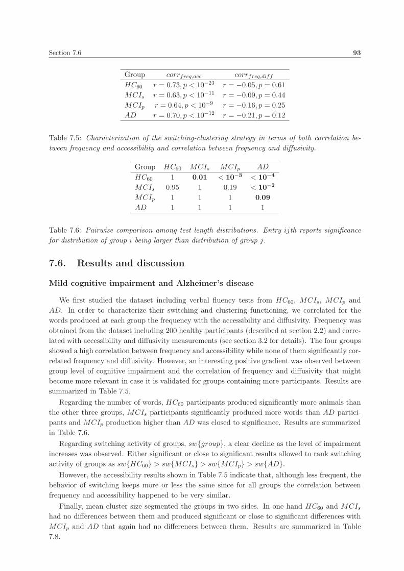
Section 7.6 93
Group corrfreq,acc corrfreq,diff
HC60 r = 0.73, p < 10−23 r = −0.05, p = 0.61
MCIs r = 0.63, p < 10−11 r = −0.09, p = 0.44
MCIp r = 0.64, p < 10−9 r = −0.16, p = 0.25
AD r = 0.70, p < 10−12 r = −0.21, p = 0.12
Table 7.5: Characterization of the switching-clustering strategy in terms of both correlation be-
tween frequency and accessibility and correlation between frequency and diffusivity.
Group HC60 MCIs MCIp AD
HC60 1 0.01 < 10−3 < 10−4
MCIs 0.95 1 0.19 < 10−2
MCIp 1 1 1 0.09
AD 1 1 1 1
Table 7.6: Pairwise comparison among test length distributions. Entry ijth reports significance
for distribution of group i being larger than distribution of group j.
7.6. Results and discussion
Mild cognitive impairment and Alzheimer’s disease
We first studied the dataset including verbal fluency tests from HC60, MCIs, MCIp and
AD. In order to characterize their switching and clustering functioning, we correlated for the
words produced at each group the frequency with the accessibility and diffusivity. Frequency was
obtained from the dataset including 200 healthy participants (described at section 2.2) and corre-
lated with accessibility and diffusivity measurements (see section 3.2 for details). The four groups
showed a high correlation between frequency and accessibility while none of them significantly cor-
related frequency and diffusivity. However, an interesting positive gradient was observed between
group level of cognitive impairment and the correlation of frequency and diffusivity that might
become more relevant in case it is validated for groups containing more participants. Results are
summarized in Table 7.5.
Regarding the number of words, HC60 participants produced significantly more animals than
the other three groups, MCIs participants significantly produced more words than AD partici-
pants and MCIp production higher than AD was closed to significance. Results are summarized
in Table 7.6.
Regarding switching activity of groups, sw{group}, a clear decline as the level of impairment
increases was observed. Either significant or close to significant results allowed to rank switching
activity of groups as sw{HC60} > sw{MCIs} > sw{MCIp} > sw{AD}.
However, the accessibility results shown in Table 7.5 indicate that, although less frequent, the
behavior of switching keeps more or less the same since for all groups the correlation between
frequency and accessibility happened to be very similar.
Finally, mean cluster size segmented the groups in two sides. In one hand HC60 and MCIs
had no differences between them and produced significant or close to significant differences with
MCIp and AD that again had no differences between them. Results are summarized in Table
7.8.
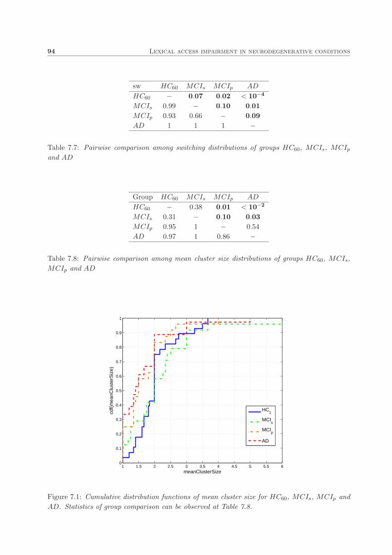
94 Lexical access impairment in neurodegenerative conditions
sw HC60 MCIs MCIp AD
HC60 − 0.07 0.02 < 10−4
MCIs 0.99 − 0.10 0.01
MCIp 0.93 0.66 − 0.09
AD 1 1 1 −
Table 7.7: Pairwise comparison among switching distributions of groups HC60, MCIs, MCIp
and AD
Group HC60 MCIs MCIp AD
HC60 − 0.38 0.01 < 10−2
MCIs 0.31 − 0.10 0.03
MCIp 0.95 1 − 0.54
AD 0.97 1 0.86 −
Table 7.8: Pairwise comparison among mean cluster size distributions of groups HC60, MCIs,
MCIp and AD
1 1.5 2 2.5 3 3.5 4 4.5 5 5.5 60
0.1
0.2
0.3
0.4
0.5
0.6
0.7
0.8
0.9
1
meanClusterSize
cdf(
mea
nClu
ster
Siz
e)
HC1
MCIs
MCIp
AD
Figure 7.1: Cumulative distribution functions of mean cluster size for HC60, MCIs, MCIp and
AD. Statistics of group comparison can be observed at Table 7.8.
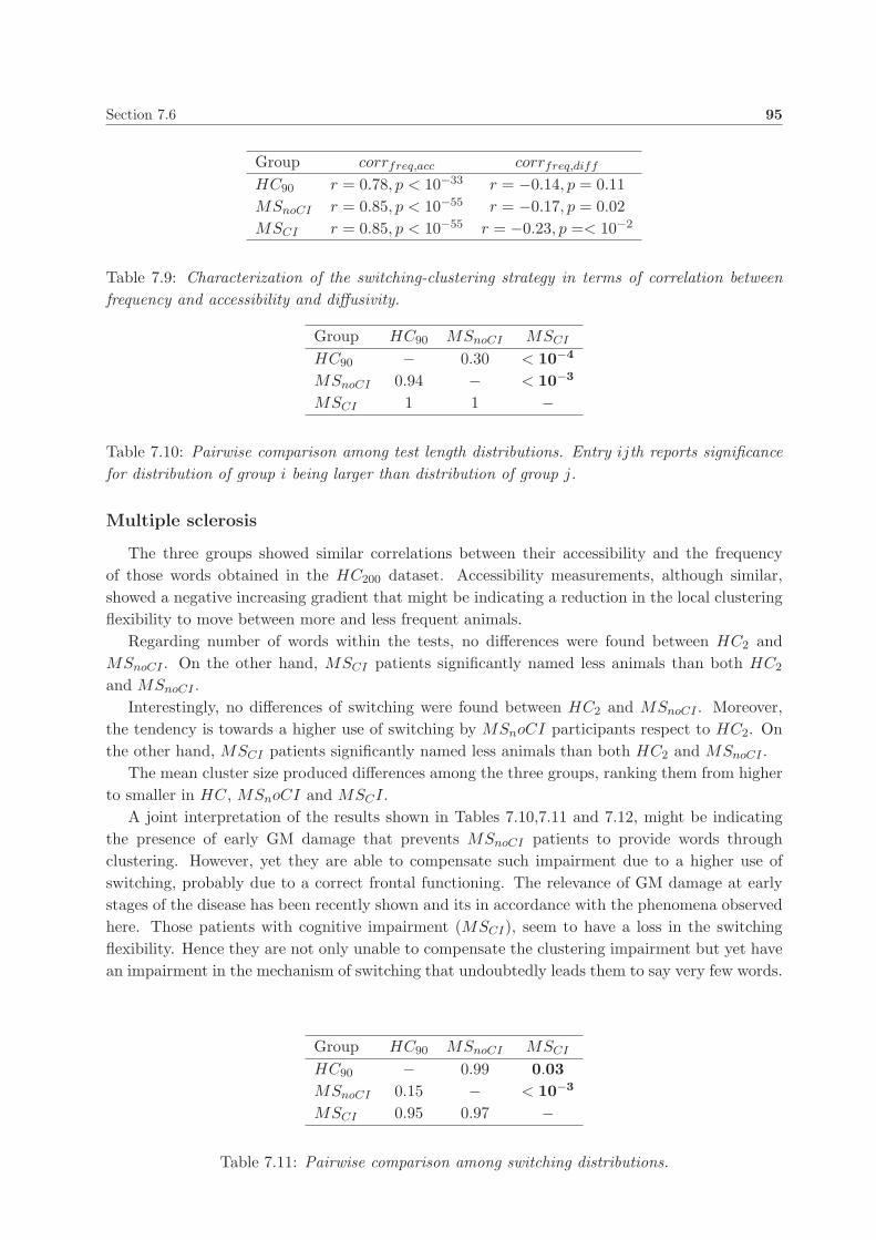
Section 7.6 95
Group corrfreq,acc corrfreq,diff
HC90 r = 0.78, p < 10−33 r = −0.14, p = 0.11
MSnoCI r = 0.85, p < 10−55 r = −0.17, p = 0.02
MSCI r = 0.85, p < 10−55 r = −0.23, p =< 10−2
Table 7.9: Characterization of the switching-clustering strategy in terms of correlation between
frequency and accessibility and diffusivity.
Group HC90 MSnoCI MSCI
HC90 − 0.30 < 10−4
MSnoCI 0.94 − < 10−3
MSCI 1 1 −
Table 7.10: Pairwise comparison among test length distributions. Entry ijth reports significance
for distribution of group i being larger than distribution of group j.
Multiple sclerosis
The three groups showed similar correlations between their accessibility and the frequency
of those words obtained in the HC200 dataset. Accessibility measurements, although similar,
showed a negative increasing gradient that might be indicating a reduction in the local clustering
flexibility to move between more and less frequent animals.
Regarding number of words within the tests, no differences were found between HC2 and
MSnoCI . On the other hand, MSCI patients significantly named less animals than both HC2
and MSnoCI .
Interestingly, no differences of switching were found between HC2 and MSnoCI . Moreover,
the tendency is towards a higher use of switching by MSnoCI participants respect to HC2. On
the other hand, MSCI patients significantly named less animals than both HC2 and MSnoCI .
The mean cluster size produced differences among the three groups, ranking them from higher
to smaller in HC, MSnoCI and MSCI.
A joint interpretation of the results shown in Tables 7.10,7.11 and 7.12, might be indicating
the presence of early GM damage that prevents MSnoCI patients to provide words through
clustering. However, yet they are able to compensate such impairment due to a higher use of
switching, probably due to a correct frontal functioning. The relevance of GM damage at early
stages of the disease has been recently shown and its in accordance with the phenomena observed
here. Those patients with cognitive impairment (MSCI), seem to have a loss in the switching
flexibility. Hence they are not only unable to compensate the clustering impairment but yet have
an impairment in the mechanism of switching that undoubtedly leads them to say very few words.
Group HC90 MSnoCI MSCI
HC90 − 0.99 0.03
MSnoCI 0.15 − < 10−3
MSCI 0.95 0.97 −
Table 7.11: Pairwise comparison among switching distributions.

96 Lexical access impairment in neurodegenerative conditions
Group HC90 MSnoCI MSCI
HC90 − < 10−2 < 10−2
MSnoCI − 1 0.06
MSCI 1 0.99 −
Table 7.12: Pairwise comparison among mean cluster size distributions.
1 1.5 2 2.5 3 3.5 4 4.5 50
0.1
0.2
0.3
0.4
0.5
0.6
0.7
0.8
0.9
1
meanClusterSize
CD
F(m
eanC
lust
erS
ize)
HCMS
noCI
MSCI
Figure 7.2: Cumulative distribution functions of mean cluster size for HC90, MSnoCI and MSCI .
Statistics of group comparison can be observed at Table 7.12.

97
Chapter 8
Conclusions and Outlook
8.1. Conclusions
The conclusions of this work are diverse, all of them centered on understanding conceptual
storage and retrieval in semantic memory as a complex system.
In chapter 2, we have seen that frequency distribution of words in semantic verbal fluency tests
(animals) follow an exponential distribution, instead of the power-law that had been previously
observed in natural language. Additionally, we have observed that more frequent words tend to
appear earlier within the tests, a phenomenon already observed in previous studies of verbal flu-
ency. These two observations have been complemented with the word heterogeneity measurement
for three different intervals of the tests. Results indicate that a joint tendency of participants to
name the same set of animals is gradually lost as the test advances.
In chapter 3, we have developed a methodology to infer an unsupervised network of concepts.
Based on a verbal fluency dataset, a network containing animal concepts (nodes) and its relations
(links) has been obtained. This network showed a strong modularity that partitioned the nodes
into 18 modules. We later used this information to enreach the network by converting each
module into a fully connected set of nodes, giving rise to an enreached conceptual network. We
used both in-silico networks as unsupervised evaluators of switching and clustering. The latter
network happened to be closer than the original one to human evaluation. Hence we used the
enreached conceptual network to decouple switching and clustering transitions by means of two
measurements, switching and clustering. Correlating these two measurements with frequency of
the concepts produced the following finding: the frequency heterogeneity studied in chapter 2 is
due to switching, while clustering has the flexibility to move from frequent to in frequent concepts
in a way similar to a random-walk.
In chapter 4 we evaluated the exploration performance of different modalities of switcher
random walks in a number of well known in-silico network models. Frequency of concepts as a
gradient was substituted by degree of nodes. Three variants of switching (no gradient, positive
degree gradient and negative degree gradient) were studied, showing different behaviors depending
on the topology explored and the level of switching.
In chapter 5, we used the switching-clustering functioning and the conceptual network ECN
obtained in chapter 3 together with the theoretical framework described in chapter 4. We analyzed
the performance of explorability for different levels of switching activity and found that there is
an optimal intermediate region, which is indeed the region where humans are. The results of
our simulations showed that switching is crucial for an optimized exploration of the conceptual
network in particular, and probably of modular networks in general.

98 Conclusions and Outlook
In chapter 6 we demonstrated that frequency of concepts in verbal fluency is a reliable estimator
of ranked age of acquisition of concepts. In other words, concepts with higher frequency in the
tests were learnt before than those concepts with lower frequency. Hence we used frequency
to model the dynamical evolution of the enreached conceptual network. This study allowed to
observe that a giant connected component that included around 80% of concepts emerged much
earlier than expected when adding nodes randomly. Such giant connected component represented
a conceptual skeleton that was later fed by filling every semantic field with more terms, giving
rise to a delayed modularity and clusterization respect to the expected by chance.
In chapter 7, four different neurodegenerative conditions were studied: Mild Cognitive Im-
pairment (stable and progressive), Alzheimer’s disease and Multiple Sclerosis (with and with-
out cognitive impairment). Patients with MCIs showed what could be an overall ralentiza-
tion of concept retrieval, while MCIp group was clearly identified as a middle stage towards
AD development. Although clustering seems to show a gradient towards loosing flexibility
(HC− > MCIs− > MCIp− > AD), a higher number of tests would be needed to accurately
make this claim. Regarding MS, patients with no cognitive impairment compensated certain
clustering impairment with an overuse of switching. Finally, those MS patients with cognitive
impairment not only showed a high clustering impairment but also had a switching impairment
that avoided any compensatory mechanism.
8.2. Outlook
It is widely accepted that clustering retrieves series of related animals while switching produces
a change to explore other sub-categories or semantic modules, and those changes have been said to
happen when categories get exhausted [31]. However, normal participants said around 31 animals
during the 90 seconds task. Globally, it is obvious that those numbers do not demonstrate the
animals lexicon that participants know but represents only a low portion of them. Regarding
subcategories, the fact that they are not exhaustively explored and retrieved might be due to
a combination different reasons. First, switching is a mechanism that naturally prevents from
exhaustive exploration of the semantic modules defined in section 3.3 in a row, and second, there
might be inhibitory mechanisms that prevents from re-visiting modules already explored. In
other words, is not only that switching abandons current sub-category (i.e. cervidae) to explore
somewhere else but it also might happen that such module might be somehow de-activated or
inhibited for a while to naturally avoid repetitions. This phenomenon might also explain why
sometimes participants, after briefly exploring several sub-catecories , get blocked for periods
of several seconds even though they only had named 15 or less animals. Indeed, the timing is
definitely the next variable to include in order to better understand the complexity of switching
and clustering phenomena and their bottlenecks.
In section 3.4 an unsupervised in-silico evaluator of switching and clustering has been proposed.
Although its performance was in high agreement with human expertise, it still lacks an evaluation
for those concepts not included in the network. This issue might be softened by considerably in-
creasing the number of verbal fluency tests included in the inference of the network. Additionally,
a selective semi-supervised evaluation could be addressed, where only those concepts unknown
for the network would be evaluated in terms of switching and clustering by human judges.
Switcher random walks might be accurate models of social networks to study propagation
phenomena such as virus spreading. In this metaphor, the basal topology would represent a
social network were nodes (individuals) directly linked are some how related and switching is a
Section 8.2 99
probabilistic mechanism that considers very sporadic (and thus not included in the social network)
contacts with other people (e.g. people you find at the airport). The paradigm of SRW applied
to this context seems to be more flexible to real life contacts and thus might be of interest for
understanding issues such as virus and diseases spreading, propagation of information, etc.
In chapters 4 and 5 we evaluated the exploration performance of SRW variants on in-silico
network models and on the conceptual network ECN respectively. The performances were mea-
sured by 〈MFPT 〉net, which is based on the mean first passage time for every pair of nodes 〈tij〉
with i 6= j (i.e. the 〈tii〉 entries, which represent the return times [198], were not considered).
A possible extension of the work presented here might study the influence of switching in maxi-
mizing the return times for different network models. Exploration strategies that maximize the
return times are very interesting from a cognitive perspective, since it reduces the probabilities of
re-visiting nodes and thus might be reducing the minimal working memory size needed to avoid
repetitions. It might be a reason for the so called magical numbers of 7 [8] or 4 [9] or at least it
might explain some cognitive limitations.
Finally, the use of switcher random walks introduced in sections 4 and 5 might be extrapolated
as a novel cognitive inspired Computer Science paradigm to find adequate solutions to complex
problems, such as the so called NP problems, where brute-force, i.e. analyzing all possible solu-
tions, is not computationally feasible. In particular, it would be of interest to evaluate SRW for
a set of known problems using different switching probabilities and to compare their performance
to other approximation algorithms such as simulated annealing [199, 200] and genetic algorithms
[201, 202]. In this context, clustering would represent a movement to a nearby solution while
switching would be a change to any other solution and several variants could be explored by
using different switching gradients.

100 Conclusions and Outlook

101
Appendix A
Words and their frequency in the 200
verbal fluency tests

102 Words and their frequency in the 200 verbal fluency tests
Table A.1: Frequency and averaged position of words in the dataset containing verbal fluency
tests (animals) from 200 healthy participants
Spanish term frequency averaged position
abeja 36 23.42
abejaruco 1 14.00
abejorro 3 27.33
abubilla 3 20.33
acaro 3 18.67
agapurni 1 28.00
aguila 75 18.07
aguila culebrera 1 30.00
aguila real 5 30.40
aguilucho 2 30.50
alacran 2 21.50
albatros 1 19.00
alce 4 37.00
alimoche 1 2.00
almeja 11 24.91
alpaca 1 30.00
ameba 1 29.00
anaconda 2 21.00
anade real 1 19.00
anchoa 10 26.80
anemona de mar 1 26.00
anguila 4 26.50
angula 2 28.00
ansar comun 1 18.00
antılope 4 23.25
arana 57 19.77
ardilla 32 15.22
arenque 3 16.67
armadillo 1 22.00
asno 9 13.89
atun 23 20.70
ave 1 10.00
ave carronera 1 39.00
ave del paraıso 1 29.00
ave lira 1 11.00
avefrıa 1 6.00
avestruz 47 15.26
avirrojo 1 7.00
avispa 24 24.68
avutarda 3 11.33
azor 1 20.00
babosa 2 14.00

103
Table A.2: Frequency and averaged position of words in the dataset containing verbal fluency
tests (animals) from 200 healthy participants
Spanish term frequency averaged position
babuino 2 32.00
bacalao 9 20.56
bacteria 2 29.00
ballena 119 16.98
barbo 8 25.25
barracuda 1 23.00
berberecho 1 23.00
besugo 10 25.00
bıgaro 1 33.00
bisonte 15 22.67
boa 10 20.40
bogavante 3 27.33
bonito 5 22.60
boqueron 1 29.00
bravia 1 17.00
buey 19 21.95
buey de mar 5 22.20
bufalo 20 23.30
buho 23 22.57
buitre 42 22.14
buitre leonado 1 47.00
burro 43 17.07
caballito de mar 12 23.17
caballo 103 12.06
cabra 56 17.98
cabrito 2 13.00
cacatua 17 18.65
cachalote 12 23.92
caiman 14 19.29
calamar 16 24.38
calandria 1 23.00
camaleon 14 17.13
camaron 2 25.00
camello 20 15.70
canario 47 13.77
cangrejo 25 24.08
canguro 31 17.63
caniche 1 6.00
caracol 11 19.45
carbonero 1 22.00
cardelina 1 3.00
caribu 2 24.50
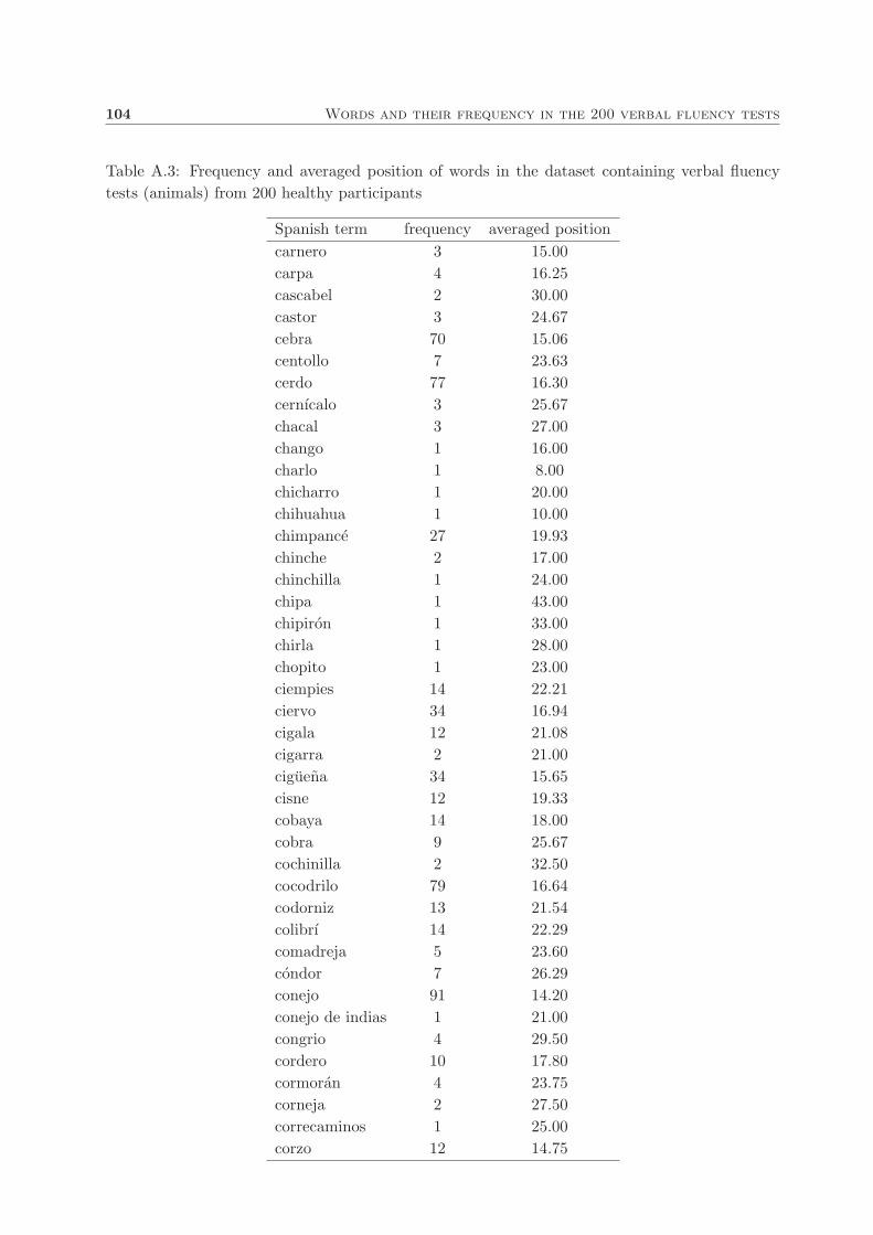
104 Words and their frequency in the 200 verbal fluency tests
Table A.3: Frequency and averaged position of words in the dataset containing verbal fluency
tests (animals) from 200 healthy participants
Spanish term frequency averaged position
carnero 3 15.00
carpa 4 16.25
cascabel 2 30.00
castor 3 24.67
cebra 70 15.06
centollo 7 23.63
cerdo 77 16.30
cernıcalo 3 25.67
chacal 3 27.00
chango 1 16.00
charlo 1 8.00
chicharro 1 20.00
chihuahua 1 10.00
chimpance 27 19.93
chinche 2 17.00
chinchilla 1 24.00
chipa 1 43.00
chipiron 1 33.00
chirla 1 28.00
chopito 1 23.00
ciempies 14 22.21
ciervo 34 16.94
cigala 12 21.08
cigarra 2 21.00
ciguena 34 15.65
cisne 12 19.33
cobaya 14 18.00
cobra 9 25.67
cochinilla 2 32.50
cocodrilo 79 16.64
codorniz 13 21.54
colibrı 14 22.29
comadreja 5 23.60
condor 7 26.29
conejo 91 14.20
conejo de indias 1 21.00
congrio 4 29.50
cordero 10 17.80
cormoran 4 23.75
corneja 2 27.50
correcaminos 1 25.00
corzo 12 14.75

105
Table A.4: Frequency and averaged position of words in the dataset containing verbal fluency
tests (animals) from 200 healthy participants
Spanish term frequency averaged position
cotorra 1 24.00
coyote 4 15.00
cucaracha 34 21.33
cuervo 19 18.63
culebra 23 12.83
delfın 82 15.44
dingo 1 26.00
dinosaurio 3 8.67
dodo 2 25.00
dorada 5 21.00
dragon de comodo 1 21.00
dromedario 10 16.30
elefante 123 11.05
elefante marino 3 35.67
emperador 1 18.00
equidna 4 28.00
erizo 8 19.88
erizo de mar 3 29.33
escarabajo 21 18.95
escolopendra 1 26.00
escorpion 12 21.83
esponja 1 37.00
estornino 1 11.00
estrella de mar 11 21.91
esturion 1 21.00
faisan 6 27.67
flamenco 4 10.25
foca 27 21.63
frailecillo 1 30.00
fuına 1 32.00
gacela 16 18.00
galapago 3 13.67
galgo 1 17.00
gallina 98 14.34
gallo 43 14.00
gamba 11 28.27
gamo 5 18.00
ganso 12 19.50
garceta 1 44.00
garrapata 4 23.25
garza 2 24.50
gato 180 6.28

106 Words and their frequency in the 200 verbal fluency tests
Table A.5: Frequency and averaged position of words in the dataset containing verbal fluency
tests (animals) from 200 healthy participants
Spanish term frequency averaged position
gato montes 1 33.00
gato pardo 1 12.00
gavilan 3 11.33
gaviota 24 14.48
gazapo 1 8.00
golondrina 17 15.72
gorila 23 20.00
gorrın 2 26.50
gorrion 49 19.22
grajo 1 28.00
grillo 6 18.00
grulla 1 11.00
guacamayo 2 13.50
gualabi 1 29.00
guepardo 39 16.62
gusano 29 19.27
gusano de seda 3 27.67
halcon 32 19.53
hamster 29 19.52
hiena 22 15.82
hipopotamo 57 17.37
hormiga 49 17.96
humano 5 22.00
huron 11 19.55
iguana 23 20.78
insecto 1 15.00
insecto palo 2 31.00
jabalı 25 18.52
jaguar 12 13.50
jilguero 24 20.25
jineta 2 17.00
jirafa 121 12.79
kili 1 12.00
kiwi 2 27.50
koala 28 19.72
lagartija 36 19.08
lagarto 35 17.77
lamprea 2 9.00
langosta 10 21.10
langostino 11 22.82
lechuza 10 19.10
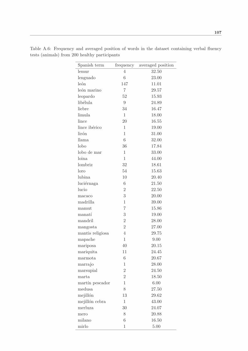
107
Table A.6: Frequency and averaged position of words in the dataset containing verbal fluency
tests (animals) from 200 healthy participants
Spanish term frequency averaged position
lemur 4 32.50
lenguado 6 23.00
leon 147 11.01
leon marino 7 29.57
leopardo 52 15.93
libelula 9 24.89
liebre 34 16.47
limula 1 18.00
lince 20 16.55
lince iberico 1 19.00
liron 1 31.00
llama 6 32.00
lobo 36 17.84
lobo de mar 1 33.00
loina 1 44.00
lombriz 32 18.61
loro 54 15.63
lubina 10 20.40
luciernaga 6 21.50
lucio 2 22.50
macaco 3 20.00
madrilla 1 39.00
mamut 7 15.86
manatı 3 19.00
mandril 2 28.00
mangosta 2 27.00
mantis religiosa 4 29.75
mapache 1 9.00
mariposa 40 20.15
mariquita 11 24.45
marmota 6 20.67
marrajo 1 28.00
marsupial 2 24.50
marta 2 18.50
martın pescador 1 6.00
medusa 8 27.50
mejillon 13 29.62
mejillon cebra 1 43.00
merluza 30 24.07
mero 8 20.88
milano 6 16.50
mirlo 1 5.00
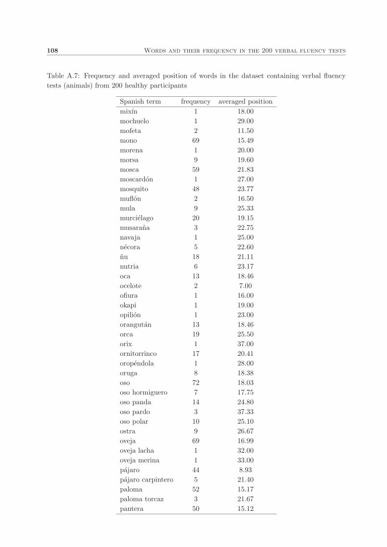
108 Words and their frequency in the 200 verbal fluency tests
Table A.7: Frequency and averaged position of words in the dataset containing verbal fluency
tests (animals) from 200 healthy participants
Spanish term frequency averaged position
mixın 1 18.00
mochuelo 1 29.00
mofeta 2 11.50
mono 69 15.49
morena 1 20.00
morsa 9 19.60
mosca 59 21.83
moscardon 1 27.00
mosquito 48 23.77
muflon 2 16.50
mula 9 25.33
murcielago 20 19.15
musarana 3 22.75
navaja 1 25.00
necora 5 22.60
nu 18 21.11
nutria 6 23.17
oca 13 18.46
ocelote 2 7.00
ofiura 1 16.00
okapi 1 19.00
opilion 1 23.00
orangutan 13 18.46
orca 19 25.50
orix 1 37.00
ornitorrinco 17 20.41
oropendola 1 28.00
oruga 8 18.38
oso 72 18.03
oso hormiguero 7 17.75
oso panda 14 24.80
oso pardo 3 37.33
oso polar 10 25.10
ostra 9 26.67
oveja 69 16.99
oveja lacha 1 32.00
oveja merina 1 33.00
pajaro 44 8.93
pajaro carpintero 5 21.40
paloma 52 15.17
paloma torcaz 3 21.67
pantera 50 15.12

109
Table A.8: Frequency and averaged position of words in the dataset containing verbal fluency
tests (animals) from 200 healthy participants
Spanish term frequency averaged position
papagayo 10 22.27
parasito 1 17.00
pato 45 15.20
pavo 13 18.77
pavo real 12 19.92
pelıcano 8 22.00
pepino de mar 1 27.00
perca 2 20.50
percebe 5 28.20
perdiz 23 16.83
perico 1 21.00
periquito 43 15.20
perro 184 4.53
perro de praderas 2 39.00
perro salchicha 1 41.00
pescadilla 2 34.00
petirrojo 6 19.83
pez 41 13.52
pez espada 25 19.04
pez gallo 5 18.00
pez manta 10 21.80
pez martillo 5 17.40
pez merlın 1 21.00
pez payaso 1 7.00
pez vela 1 11.00
picaraza 4 19.75
pichon 3 10.67
picnogonido 1 16.00
pinguino 25 23.44
pinzon 2 5.50
piojo 8 27.50
pirana 8 19.25
piton 4 26.75
polilla 2 38.00
polipo 1 25.00
pollo 47 12.55
poni 4 17.75
potro 6 15.17
protozoo 1 28.00
puercoespın 2 20.50
pulga 14 18.07
pulgon 3 21.67

110 Words and their frequency in the 200 verbal fluency tests
Table A.9: Frequency and averaged position of words in the dataset containing verbal fluency
tests (animals) from 200 healthy participants
Spanish term frequency averaged position
pulpo 25 21.44
puma 17 12.65
quebrantahuesos 8 28.75
quisquilla 1 21.00
rana 29 17.28
rape 8 19.50
rata 67 17.03
raton 91 15.17
raya 11 24.00
rebeco 3 21.67
renacuajo 1 18.00
reno 5 22.60
reptil 1 22.00
rinoceronte 68 17.36
rodaballo 3 25.00
ruisenor 6 20.67
salamandra 15 23.27
salamanquesa 2 19.50
salmon 25 22.20
salmonete 1 45.00
saltamontes 18 21.89
sanguijuela 1 33.00
sapo 15 18.38
sardina 27 22.11
sarrio 1 27.00
sepia 5 27.20
serpiente 82 17.46
siluro 2 22.50
simio 1 28.00
tabano 3 38.67
tarantula 2 19.50
tarın 1 12.00
tejon 3 18.67
tenia 1 16.00
ternero 21 13.38
tiburon 90 18.52
tiburon blanco 2 26.50
tigre 118 12.04
tigre blanco 1 35.00
tigre de bengala 1 20.00
titı 1 26.00
topillo 1 38.00

111
Table A.10: Frequency and averaged position of words in the dataset containing verbal fluency
tests (animals) from 200 healthy participants
Spanish term frequency averaged position
topo 15 23.60
tordo 1 11.00
toro 57 17.12
tortola 2 17.00
tortuga 38 17.53
triton 1 18.00
trucha 33 23.94
tucan 9 17.67
urogallo 4 26.50
urraca 3 26.67
vaca 102 13.80
venado 1 31.00
verderol 2 22.50
vıbora 9 22.00
vicuna 1 37.00
vieira 1 23.00
yegua 16 17.13
zapatero 1 16.00
zorro 35 19.05
zorzal comun 1 6.00
zorzal real 1 9.00
zurita 1 16.00

112 Words and their frequency in the 200 verbal fluency tests
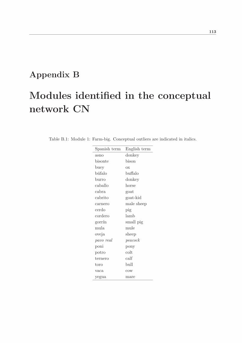
113
Appendix B
Modules identified in the conceptual
network CN
Table B.1: Module 1: Farm-big. Conceptual outliers are indicated in italics.
Spanish term English term
asno donkey
bisonte bison
buey ox
bufalo buffalo
burro donkey
caballo horse
cabra goat
cabrito goat-kid
carnero male sheep
cerdo pig
cordero lamb
gorrın small pig
mula mule
oveja sheep
pavo real peacock
poni pony
potro colt
ternero calf
toro bull
vaca cow
yegua mare

114 Modules identified in the conceptual network CN
Table B.2: Module 2: Farm- and forest-small. Conceptual outliers are indicated in italics.
Spanish term English term
ardilla squirrel
cisne swan
codorniz quail
comadreja weasel
conejo rabbit
gallina hen
gallo cock
ganso goose
liebre hare
oca domestic goose
pato duck
pavo turkey
perdiz partridge
picaraza magpie
pollo chicken
tejon badger
Table B.3: Module 3: Cervidae. Conceptual outliers are indicated in italics.
Spanish term English term
alce moose
antılope antelope
caribu caribou
ciervo deer
corzo roe deer
erizo hedgehog
gacela gazelle
gamo fallow deer
jabalı wild boar
muflon mouflon
rebeco chamois
reno reindeer
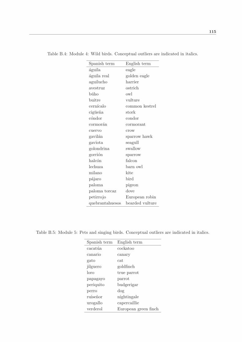
115
Table B.4: Module 4: Wild birds. Conceptual outliers are indicated in italics.
Spanish term English term
aguila eagle
aguila real golden eagle
aguilucho harrier
avestruz ostrich
buho owl
buitre vulture
cernıcalo common kestrel
ciguena stork
condor condor
cormoran cormorant
cuervo crow
gavilan sparrow hawk
gaviota seagull
golondrina swallow
gorrion sparrow
halcon falcon
lechuza barn owl
milano kite
pajaro bird
paloma pigeon
paloma torcaz dove
petirrojo European robin
quebrantahuesos bearded vulture
Table B.5: Module 5: Pets and singing birds. Conceptual outliers are indicated in italics.
Spanish term English term
cacatua cockatoo
canario canary
gato cat
jilguero goldfinch
loro true parrot
papagayo parrot
periquito budgerigar
perro dog
ruisenor nightingale
urogallo capercaillie
verderol European green finch

116 Modules identified in the conceptual network CN
Table B.6: Module 6: Crustacean and mollusc. Conceptual outliers are indicated in italics.
Spanish term English term
almeja clam
bogavante European lobster
caballito de mar sea horse
cangrejo crab
centollo spider crab
cigala Norway lobster
estrella de mar starfish
gamba prawn
langosta lobster
langostino king prawn
medusa jellyfish
mejillon mussel
necora velvet crab
ostra oyster
percebe barnacle
pulpo octopus
raya ray fish
sepia cuttlefish

117
Table B.7: Module 7: Fish. Conceptual outliers are indicated in italics.
Spanish term English term
anchoa anchovy
arenque herring
atun tuna
bacalao cod
ballena whale
barbo barb
besugo sea bream
bonito skipjack tuna
cachalote sperm whale
calamar squid
carpa carp
congrio conger
delfın dolphin
dorada hilt-head bream
lenguado sole
lubina sea bass
lucio northern pike
merluza hake
mero grouper
orca killer whale
pez fish
pez espada swordfish
pez gallo flat fish
pez martillo hammer fish
rape monkfish
rodaballo turbot
salmon salmon
sardina sardine
tiburon shark
tortuga turtle
trucha trout
Table B.8: Module 8: Unclassifiable. Conceptual outliers are indicated in italics.
Spanish term English term
pelicano pelican
pez manta manta ray

118 Modules identified in the conceptual network CN
Table B.9: Module 9: Reptiles. Conceptual outliers are indicated in italics.
Spanish term English term
boa boa
caiman alligator
camaleon chameleon
camello camel
cascabel rattle snake
cobra cobra
cocodrilo crocodile
culebra little snake
iguana iguana
lagartija wall lizard
lagarto lizard
manatı manatee
pirana piranha
piton python
rana frog
salamandra salamander
salamanquesa gecko
sapo toad
serpiente snake
tucan toucan
vibora viper
Table B.10: Module 10: Rodents. Conceptual outliers are indicated in italics.
Spanish term English term
cobaya guinea pig
dromedario dromedary
hamster hamster
rata rat
raton mouse
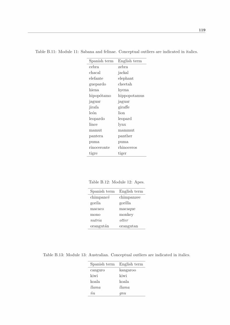
119
Table B.11: Module 11: Sabana and felinae. Conceptual outliers are indicated in italics.
Spanish term English term
cebra zebra
chacal jackal
elefante elephant
guepardo cheetah
hiena hyena
hipopotamo hippopotamus
jaguar jaguar
jirafa giraffe
leon lion
leopardo leopard
lince lynx
mamut mammut
pantera panther
puma puma
rinoceronte rhinoceros
tigre tiger
Table B.12: Module 12: Apes.
Spanish term English term
chimpance chimpanzee
gorila gorilla
macaco macaque
mono monkey
nutria otter
orangutan orangutan
Table B.13: Module 13: Australian. Conceptual outliers are indicated in italics.
Spanish term English term
canguro kangaroo
kiwi kiwi
koala koala
llama llama
nu gnu
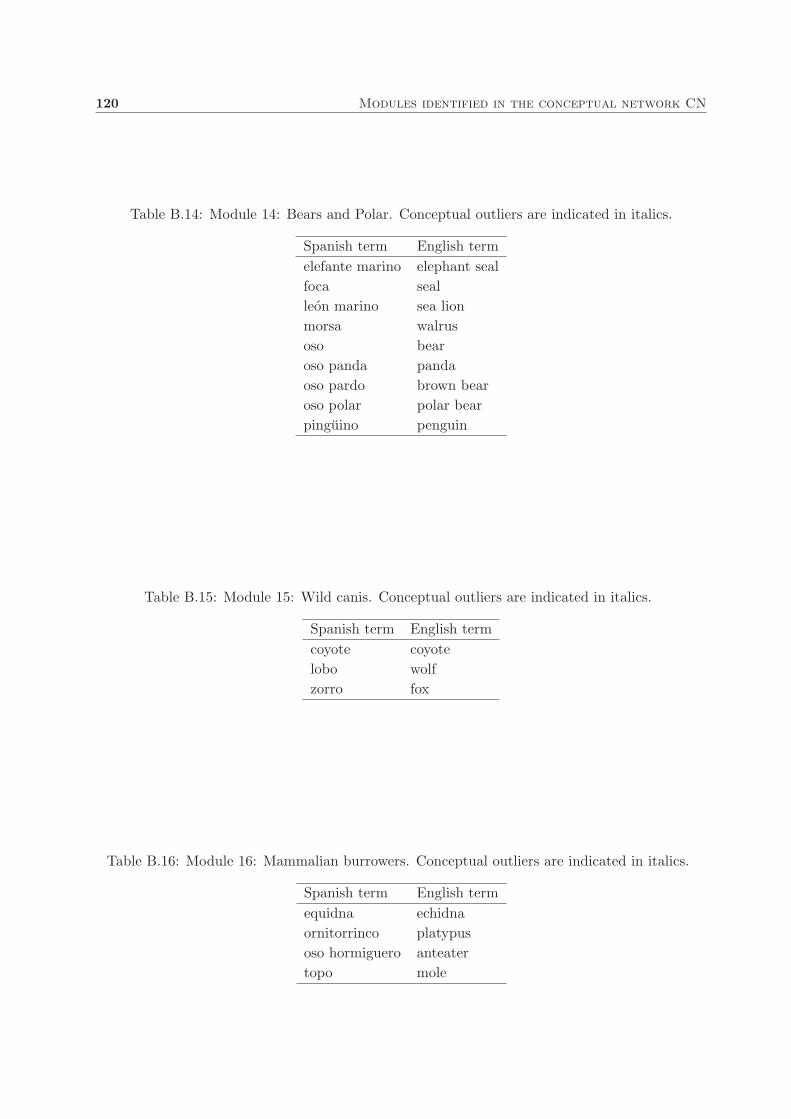
120 Modules identified in the conceptual network CN
Table B.14: Module 14: Bears and Polar. Conceptual outliers are indicated in italics.
Spanish term English term
elefante marino elephant seal
foca seal
leon marino sea lion
morsa walrus
oso bear
oso panda panda
oso pardo brown bear
oso polar polar bear
pinguino penguin
Table B.15: Module 15: Wild canis. Conceptual outliers are indicated in italics.
Spanish term English term
coyote coyote
lobo wolf
zorro fox
Table B.16: Module 16: Mammalian burrowers. Conceptual outliers are indicated in italics.
Spanish term English term
equidna echidna
ornitorrinco platypus
oso hormiguero anteater
topo mole
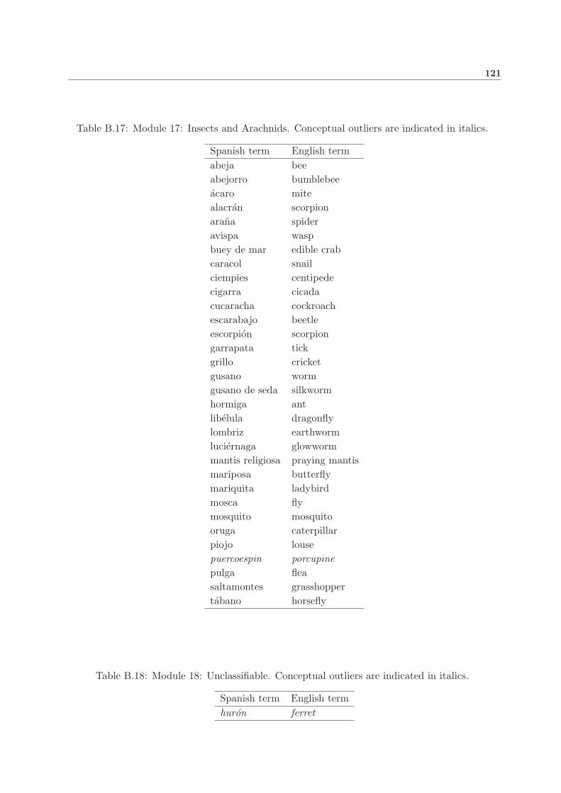
121
Table B.17: Module 17: Insects and Arachnids. Conceptual outliers are indicated in italics.
Spanish term English term
abeja bee
abejorro bumblebee
acaro mite
alacran scorpion
arana spider
avispa wasp
buey de mar edible crab
caracol snail
ciempies centipede
cigarra cicada
cucaracha cockroach
escarabajo beetle
escorpion scorpion
garrapata tick
grillo cricket
gusano worm
gusano de seda silkworm
hormiga ant
libelula dragonfly
lombriz earthworm
luciernaga glowworm
mantis religiosa praying mantis
mariposa butterfly
mariquita ladybird
mosca fly
mosquito mosquito
oruga caterpillar
piojo louse
puercoespin porcupine
pulga flea
saltamontes grasshopper
tabano horsefly
Table B.18: Module 18: Unclassifiable. Conceptual outliers are indicated in italics.
Spanish term English term
huron ferret

122 Modules identified in the conceptual network CN

123
Appendix C
Age of acquisition of animals and
their frequency in verbal fluency
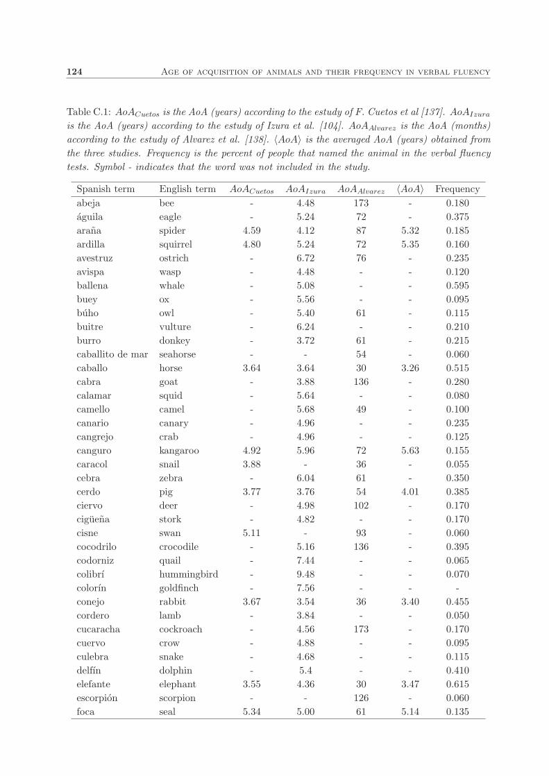
124 Age of acquisition of animals and their frequency in verbal fluency
Table C.1: AoACuetos is the AoA (years) according to the estudy of F. Cuetos et al [137]. AoAIzura
is the AoA (years) according to the estudy of Izura et al. [104]. AoAAlvarez is the AoA (months)
according to the estudy of Alvarez et al. [138]. 〈AoA〉 is the averaged AoA (years) obtained from
the three studies. Frequency is the percent of people that named the animal in the verbal fluency
tests. Symbol - indicates that the word was not included in the study.
Spanish term English term AoACuetos AoAIzura AoAAlvarez 〈AoA〉 Frequency
abeja bee - 4.48 173 - 0.180
aguila eagle - 5.24 72 - 0.375
arana spider 4.59 4.12 87 5.32 0.185
ardilla squirrel 4.80 5.24 72 5.35 0.160
avestruz ostrich - 6.72 76 - 0.235
avispa wasp - 4.48 - - 0.120
ballena whale - 5.08 - - 0.595
buey ox - 5.56 - - 0.095
buho owl - 5.40 61 - 0.115
buitre vulture - 6.24 - - 0.210
burro donkey - 3.72 61 - 0.215
caballito de mar seahorse - - 54 - 0.060
caballo horse 3.64 3.64 30 3.26 0.515
cabra goat - 3.88 136 - 0.280
calamar squid - 5.64 - - 0.080
camello camel - 5.68 49 - 0.100
canario canary - 4.96 - - 0.235
cangrejo crab - 4.96 - - 0.125
canguro kangaroo 4.92 5.96 72 5.63 0.155
caracol snail 3.88 - 36 - 0.055
cebra zebra - 6.04 61 - 0.350
cerdo pig 3.77 3.76 54 4.01 0.385
ciervo deer - 4.98 102 - 0.170
ciguena stork - 4.82 - - 0.170
cisne swan 5.11 - 93 - 0.060
cocodrilo crocodile - 5.16 136 - 0.395
codorniz quail - 7.44 - - 0.065
colibrı hummingbird - 9.48 - - 0.070
colorın goldfinch - 7.56 - - -
conejo rabbit 3.67 3.54 36 3.40 0.455
cordero lamb - 3.84 - - 0.050
cucaracha cockroach - 4.56 173 - 0.170
cuervo crow - 4.88 - - 0.095
culebra snake - 4.68 - - 0.115
delfın dolphin - 5.4 - - 0.410
elefante elephant 3.55 4.36 30 3.47 0.615
escorpion scorpion - - 126 - 0.060
foca seal 5.34 5.00 61 5.14 0.135

125
Table C.2: AoACuetos is the AoA (years) according to the estudy of F. Cuetos et al [137]. AoAIzura
is the AoA (years) according to the estudy of Izura et al. [104]. AoAAlvarez is the AoA (months)
according to the estudy of Alvarez et al. [138]. 〈AoA〉 is the averaged AoA (years) obtained from
the three studies. Frequency is the percent of people that named the animal in the verbal fluency
tests. Symbol - indicates that the word was not included in the study.
Spanish term English term AoACuetos AoAIzura AoAAlvarez 〈AoA〉 Frequency
gallina hen 3.43 3.36 43 3.46 0.490
gallo rooster - 3.52 102 - 0.215
gamba prawn - 5.72 - - 0.055
gamo fallow deer - 8.04 - - 0.025
gato cat 3.33 3.00 36 3.11 0.900
gaviota seagull - 5.08 - - 0.120
golondrina swallow - 5.04 - - 0.085
gorila gorilla - 5.60 72 - 0.115
gorrino pig - 5.32 - - 0.010
gorrion sparrow - 5.00 - - 0.245
guepardo cheetah - 7.08 - - 0.195
gusano worm - 4.00 - - 0.145
halcon falcon - 6.68 - - 0.160
hamster hamster - 7.56 - - 0.145
hiena hyena - 7.16 - - 0.110
hipopotamo hippopotamus - 6.16 - - 0.285
hormiga aunt - 4.64 102 - 0.245
iguana iguana - 9.16 - - 0.115
jabalı wild boar - 8.32 - - 0.125
jirafa giraffe 4.40 6.48 49 4.99 0.605
koala koala - 9 - - 0.140
lagartija little lizard - 5.64 - - 0.180
lagarto lizard - 6.76 - - 0.175
langostino king prawn - 8.36 - - 0.055
lechuza owl - 7.96 - - 0.05
leon lion 4.08 5.28 36 4.12 0.735
leopardo leopard - 7.16 93 - 0.260
liebre hare - 6.16 - - 0.170
lince lynx - 8.08 - - 0.100
lobo wolf - 5.44 - - 0.180
loro parrot - 6.32 - - 0.270
mapache raccoon - - 173 - 0.005
mariposa butterfly 4.42 4.84 36 4.09 0.200
mofeta skunk - - 93 - 0.010
mono monkey 4.40 4.92 43 4.30 0.345
mosca fly - 4.52 136 - 0.295
mosquito mosquito - 5.12 - - 0.240
orangutan orangutan - 7.36 - - 0.065
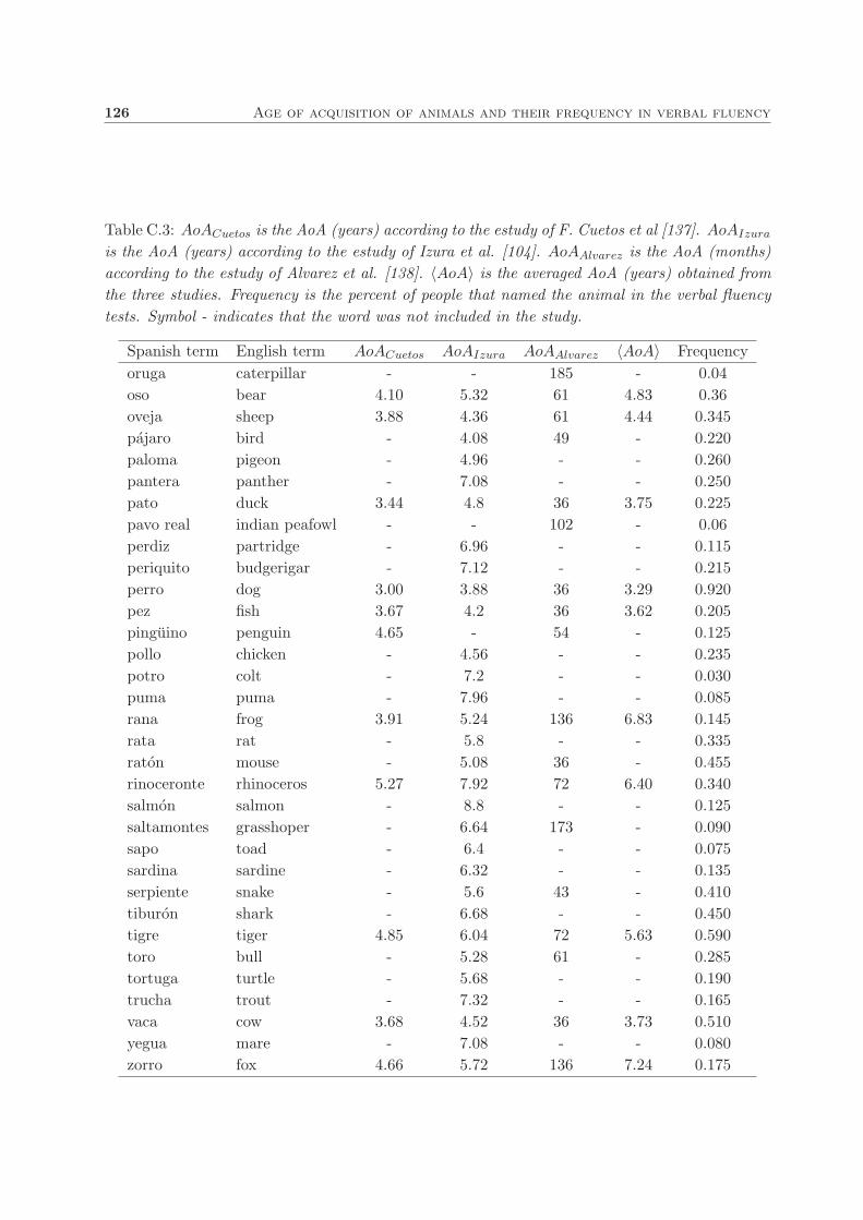
126 Age of acquisition of animals and their frequency in verbal fluency
Table C.3: AoACuetos is the AoA (years) according to the estudy of F. Cuetos et al [137]. AoAIzura
is the AoA (years) according to the estudy of Izura et al. [104]. AoAAlvarez is the AoA (months)
according to the estudy of Alvarez et al. [138]. 〈AoA〉 is the averaged AoA (years) obtained from
the three studies. Frequency is the percent of people that named the animal in the verbal fluency
tests. Symbol - indicates that the word was not included in the study.
Spanish term English term AoACuetos AoAIzura AoAAlvarez 〈AoA〉 Frequency
oruga caterpillar - - 185 - 0.04
oso bear 4.10 5.32 61 4.83 0.36
oveja sheep 3.88 4.36 61 4.44 0.345
pajaro bird - 4.08 49 - 0.220
paloma pigeon - 4.96 - - 0.260
pantera panther - 7.08 - - 0.250
pato duck 3.44 4.8 36 3.75 0.225
pavo real indian peafowl - - 102 - 0.06
perdiz partridge - 6.96 - - 0.115
periquito budgerigar - 7.12 - - 0.215
perro dog 3.00 3.88 36 3.29 0.920
pez fish 3.67 4.2 36 3.62 0.205
pinguino penguin 4.65 - 54 - 0.125
pollo chicken - 4.56 - - 0.235
potro colt - 7.2 - - 0.030
puma puma - 7.96 - - 0.085
rana frog 3.91 5.24 136 6.83 0.145
rata rat - 5.8 - - 0.335
raton mouse - 5.08 36 - 0.455
rinoceronte rhinoceros 5.27 7.92 72 6.40 0.340
salmon salmon - 8.8 - - 0.125
saltamontes grasshoper - 6.64 173 - 0.090
sapo toad - 6.4 - - 0.075
sardina sardine - 6.32 - - 0.135
serpiente snake - 5.6 43 - 0.410
tiburon shark - 6.68 - - 0.450
tigre tiger 4.85 6.04 72 5.63 0.590
toro bull - 5.28 61 - 0.285
tortuga turtle - 5.68 - - 0.190
trucha trout - 7.32 - - 0.165
vaca cow 3.68 4.52 36 3.73 0.510
yegua mare - 7.08 - - 0.080
zorro fox 4.66 5.72 136 7.24 0.175

BIBLIOGRAPHY 127
Bibliography
[1] Wikipedia. Human brain — Wikipedia, the free encyclopedia (2008). [Online; accessed
28-August-2008].
[2] The hopes brain tutorial. http://www.stanford.edu/group/hopes/basics/braintut/ab3.html
.
[3] Wikipedia. Lobes of the brain — Wikipedia, the free encyclopedia (2008). [Online; accessed
28-August-2008].
[4] Wikipedia. Homunculus — Wikipedia, the free encyclopedia (2008). [Online; accessed 08-
September-2008].
[5] Wikibooks. Consciousness studies — Wikibooks (2008). [Online; accessed 08-September-
2008].
[6] A. E. Budson, B. H. Price. Memory dysfunction. The New England Journal of Medicine
352 (7), (2005), pp. 692–699.
[7] Wikipedia. Memory — Wikipedia, the free encyclopedia (2008). [Online; accessed 28-
August-2008].
[8] G. Miller. The magical number seven, plus or minus two: Some limits on our capacity for
processing information. Psychological Review 63, (1956), pp. 81–97.
[9] N. Cowan. The magical number 4 in short-term memory: A reconsideration of mental
storage capacity. Behavioral and Brain Sciences 24, (2001), pp. 87–185.
[10] H. A. Simon. How big is a chunk? Science 183, (1974), pp. 482–488.
[11] S. Lakhan. Neuropsychological generation of source amnesia: An episodic memory disorder
of the frontal brain. Journal of Medicine 1 (1), (2007), pp. 70–74.
[12] J. R. Anderson. Language, memory and thought. Lawrence Earlbaum Associates, Hillsdale,
NJ (1976).
[13] M. K. Johnson, S. Hashtroudi. Source monitoring. Psychological Bulletin 114 (1), (1993),
pp. 3–28.
[14] E. Winograd. Some observation on prospective remembering. In M. M. Gruneberg, P. E.
Morris, R. N. Sykes, eds., Pratical aspects of memory: Current research and issues, pp.
349–353. J. Wiley and Sons, Chichester, N.Y. (1988).
[15] E. Tulving. Episodic and semantic memory. In Organization and memory, pp. 381–403.
Academic Press, New York and London (1978).

128 BIBLIOGRAPHY
[16] L. Squire. Memory and Brain. Oxford University Press, New York (1987).
[17] A. Martin. The representation of object concepts in the brain. Annual Review of Psychology
58, (2007), pp. 25–45.
[18] T. T. Rogers, A. Ivanoiu, K. Patterson, J. Hodges. Semantic memory in alzheimer’s disease
and the frontotemporal dementias: a longitudinal study of 236 patients. Neuropsychology
20 (3), (2006), pp. 319–335.
[19] K. Patterson, P. J. Nestor, T. T. Rogers. Where do you know what you know? the represen-
tation of semantic knowledge in the human brain. Nature Reviews Neuroscience 8, (2007),
pp. 976–987.
[20] P. Poulin, K. Zakzanis. In vivo neuroanatomy of alzheimer’s disease: evidence from struc-
tural and functional brain imaging. Brain and Cognition 49 (2), (2002), pp. 220–225.
[21] R. Davies, G. Halliday, J. Xuereb, J. Kril, J. Hodges. The neural basis of semantic memory:
Evidence from semantic dementia. Neurobiology of aging p. in press.
[22] M. F. Newman, J. L. Kirschner, B. Philips-Bute, V. Gaver, H. Grocott, R. H. Jones, D. B.
Mark, J. G. Reves, J. A. Blumenthal. Longitudinal assessment of neurocognitive function
after coronary-artery bypass surgery. New England Journal of Medicine 344, (2001), pp.
395–402.
[23] M. Mesulman. Principles of behavioral and cognitive neurology. 2nd edition. Oxford Uni-
versity Press, New York (2000).
[24] M. Galeote, H. Peraita. Memoria semantica y fluidez verbal en demencias. Revista Espanola
de Neuropsicologıa 1 (2-3), (1999), pp. 3–17.
[25] A. Ardila, F. Ostrosky-Solıs. Cognitive testing toward the future: The example of semantic
verbal fluency (animals). International Journal of Psychology 41 (5), (2006), pp. 324–332.
[26] M. Lezak. Neuropsychological assessment. 3rd edition. Oxford University Press, New York
(1995).
[27] W. Bousfield, C. Sedgewick. An analysis of sequences of restricted associative responses.
Journal of General Psychology 30, (1944), pp. 149–165.
[28] P. Gruenewald, G. Lockhead. The free recall of category examples. Journal of Experimental
Psychology: Human Learning and Memory 6 (3), (1980), pp. 225–240.
[29] S. Raskin, M. Sliwinski, J. Borod. Clustering strategies on tasks of verbal fluency in parkin-
son’s disease. Neuropsychologia 30 (1), (1992), pp. 95–99.
[30] J. Wixted, D. Rohrer. Analyzing the dynamics of free recall: An integrative review of the
empirical literature. Psychonomic Bulletin and Review 1 (1), (1994), pp. 89–106.
[31] A. K. Troyer, M. Moscovitch, G. Winocur. Clustering and switching as two components of
verbal fluency: Evidence from younger and older healthy adults. Neuropsychology 11 (1),
(1997), pp. 138–146.
[32] A. K. Troyer, M. Moscovitch, G. Winocur, M. P. Alexander, D. Stuss. Clustering and
switching on verbal fluency: the effect of focal frontal- and temporal-lobe lesions. Neuropsy-
chologia 36 (6), (1998), pp. 499–504.

BIBLIOGRAPHY 129
[33] A. K. Troyer, M. Moscovitch, G. Winocur, L. Leach, M. Freedman. Clustering and switching
on verbal fluency tests in alzheimer’s and parkinson’s disease. Journal of the International
Neuropsychological Society 4 (2), (1998), pp. 137–143.
[34] A. Troster, J. Fields, J. Testa, R. Paul, C. Blanco, K. Hames, D. Salmon, W. Beatty.
Cortical and subcortical influences on clustering and switching in the performance of verbal
fluency tasks. Neuropsychologia 36 (4), (1998), pp. 295–304.
[35] H. Jeong, S. Mason, A. Barabasi, Z. Oltvai. Lethality and centrality in protein networks.
Nature 411 (6833), (2001), pp. 41–42.
[36] A. Wagner. The yeast protein interaction network evolves rapidly and contains few redun-
dant duplicate genes. Molecular Biology Evolution 18 (7), (2001), pp. 1283–1292.
[37] R. V. Sole, R. Pastor-Satorras, E. Smith, T. Kepler. A model of large-scale proteome
evolution. Advances in Complex Systems 5, (2003), pp. 43–54.
[38] J. Goni, F. Esteban, N. V. de Mendizabal, J. Sepulcre, S. Ardanza-Trevijano, I. Agirrez-
abal, P. Villoslada. A computational analysis of protein-protein interaction networks in
neurodegenerative diseases. BMC Systems Biology p. in press.
[39] R. Palacios, J. Goni, I. Martinez-Forero, J. Iranzo, J. Sepulcre, I. Melero, P. Villoslada. A
network analysis of the human t-cell activation gene network identifies jagged1 as a thera-
peutic target for autoimmune diseases. PLoS ONE 2 (11), (2007), p. e1222.
[40] B. K. Chakrabarti, A. Chakraborti, A. Chatterjee, eds. Econophysics and Sociophysics:
Trends and Perspectives. Raven Press (2006).
[41] G. Palla, A. Barabasi, T. Vicksek. Quantifying social group evolution. Nature 446 (7136),
(2007), pp. 664–667.
[42] L. W. Ancel, M. J. Newman, M. Martin, S. Schrag. Applying network theory to epidemics:
Control measures for outbreaks of mycoplasma pneumoniae, emerging infectious diseases 9.
J. Epidemiol 9, (2001), pp. 204–210.
[43] M. Keeling, K. Eames. Networks and epidemic models. Journal of the Royal Society,
Interface / the Royal Society 2 (4), (2005), pp. 295–307.
[44] A. Capocci, G. Caldarelli, R. Marchetti, L. Pietronero. Growing dynamics of internet
providers. Physical Review E .
[45] R. Pastor-Satorras, A. Vazquez, A. Vespignani. Dynamical and correlation properties of the
internet. Phys Rev E Stat Nonlin Soft Matter Phys 87, (2001), p. 258701.
[46] R. Ferrer i Cancho, R. V. Sole. The small world of human language. Proceedings of the
Royal Society of London. Series B, Biological Sciences 268 (1482), (2001), pp. 2261–2265.
[47] R. Ferrer i Cancho, R. V. Sole, R. Koler. Patterns in syntactic dependency networks.
Physical Review E 69 (051915).
[48] S.-J. Yang. Exploring complex networks by walking on them. Physical Review E 71, (2005),
p. 016107.
[49] R. Albert, H. Jeong, A. Barabasi. Error and attack tolerance of complex networks. Nature
406 (6794), (2000), pp. 378–382.

130 BIBLIOGRAPHY
[50] D. Callaway, M. Newman, D. Watts. Network robustness and fragility: percolation on
random graphs. Physical Review Letter 85 (25), (2000), pp. 5468–5471.
[51] R. Cohen, K. Erez, D. ben Avraham, S. Havlin. Resilience of the internet to random
breakdowns. Physical Review Letters 85 (21), (2000), pp. 4626–4628.
[52] R. Cohen, K. Erez, D. ben Avraham, S. Havlin. Breakdown of the internet under intentional
attack. Physical Review Letters 86 (16), (2001), pp. 3682–3685.
[53] R. Albert, A.-L. Barabasi. Statistical mechanics of complex networks. Reviews of Modern
Physics 74 (47).
[54] O. Mason, M. Verwoerd. Graph theory and networks in biology. IET Systems Biology 1 (2),
(2007), pp. 89–119.
[55] M. Shlesinger. Mathematical physics: search research. Nature 443 (7109), (2006), pp.
281–282.
[56] Wikipedia. Random walk — Wikipedia, the free encyclopedia (2008). [Online; accessed
09-September-2008].
[57] J. D. Noh, H. Rieger. Random walks on complex networks. Physical Review Letters 92 (11).
[58] M. Rosvall, C. T. Bergstrom. Maps of random walks on complex networks reveal community
structure. Proceedings of the National Academy of Sciences of the United States of America
105 (4), (2008), pp. 1118–1123.
[59] S. Jespersen, I. Sokolov, A. Blumen. Relaxation properties of small-world networks. Phys
Rev E Stat Nonlin Soft Matter Phys 62, (2000), pp. 4405–4408.
[60] R. Guimera, A. Dıaz-Guilera, F. Vega-Redondo, A. Cabrales, A. Arenas. Optimal network
topologies for local search with congestion. Physical Review Letters 89, (2002), p. 248701.
[61] N. M. Henley. A psychological study of the semantics of animal terms. Journal of Verbal
Learning and Verbal Behavior 8, (1969), pp. 176–184.
[62] L. Li, D. Alderson, J. C. Doyle, W. Willinger. Towards a theory of scale-free graphs:
Definition, properties, and implications. Internet Mathematics 2 (4), (2006), pp. 431–523.
[63] A. Clauset, C. R. Shalizi, M. E. J. Newman. Power-law distributions in empirical data
(2007).
[64] R. Shepard. Toward a universal law of generalization for psychological science. Science
237 (4820), (1987), pp. 1317–1323.
[65] L. Royer, S. Pouvreau, E. Rios. Evolution and modulation of intracellular calcium release
during long-lasting, depleting depolarization in mouse muscle. Journal of Physiology p. in
press.
[66] G. Zipf. The psycho-biology of language. Houghton Mifflin, New York (1935).
[67] V. Balasubrahmanyan, S. Naranan. Quantitative linguistics and complex system studies.
Journal of Quantitative Linguistics 3 (3), (1996), pp. 177–228.
[68] E. Rosch. Cognitive representations of semantic categories. Journal of Experimental Psy-
chology: General 104 (3), (1975), pp. 192–233.
BIBLIOGRAPHY 131
[69] E. Rosch, C. Simpson, R. S. Miller. Structural bases of tipicality. Journal of Experimental
Psychology: Human perception and Performance 2 (4), (1976), pp. 491–502.
[70] W. Bousfield, W. Barclay. The relationship between order and frequency of occurrence of
restricted associative responses. Journal of Experimental Psychology 40 (5), (1950), pp.
643–647.
[71] S. Wasserman, K. Faust. Social Network Analysis: Methods and Applications. Cambridge
University Press (1994).
[72] B. Voy, J. Scharff, A.D.Perkins, A. Saxton, B. Borate, E. Chesler, L. Branstetter,
M. Langston. Extracting gene networks for low-dose radiation using graph theoretical algo-
rithms. Plos Computational Biology 2 (7), (2006), p. e89.
[73] M. Sigman, G. Cecchi. Global organization of the wordnet lexicon. PNAS 99 (3), (2002),
pp. 1742–1747.
[74] A. E. Motter, A. P. de Moura, Y.-C. Lan, P. Dasgupta. Topology of the conceptual network
of language. Physical Review E 65 (065102).
[75] M. Steyvers, J. B. Tenenbaum. The large-scale structure of semantic networks: Statistical
analyses and a model of semantic growth. Cognitive Science 29, (2005), pp. 41–78.
[76] A. M. Collins, M. R. Quillian. Retrieval time from semantic memory. Journal of verbal
learning and verbal behavior 8 (2), (1969), pp. 240–248.
[77] A. M. Collins, M. R. Quillian. Does category size affect categorization time? Journal of
verbal learning and verbal behavior 9 (4), (1970), pp. 432–438.
[78] S. A. Sloman. Categorical inference is not a tree: The myth of inheritance hierarchies.
Cognitive Psychology 35, (1998), pp. 1–33.
[79] M. R. Quillian. Word concepts: A theory and simulation of some basic semantic capabilities.
Behavioral Science 12 (5), (1967), pp. 410–430.
[80] A. M. Collins, E. F. Loftus. A spreading-activation theory of semantic processing. Psycho-
logical Review 82 (6), (1975), pp. 407–428.
[81] B. Hayes-Roth. Evolution of cognitive structures and processes. Psychological Review
84 (3), (1977), pp. 260–278.
[82] J. R. Anderson, P. L. Pirolli. Spread of activation. Journal of Experimental Psychology:
learning Memory and Cognition 10 (4), (1984), pp. 791–798.
[83] T. L. Griffiths, M. Steyvers, J. B. Tenenbaum. Topics in semantic representation. Psycho-
logical Review 114 (2), (2007), pp. 211–244.
[84] L. J. Rips, E. J. Shoben, E. E. Smith. Semantic distance and the verification of semantic
relations. Journal of Verbal Learning and Verbal Behavior 12, (1973), pp. 1–20.
[85] S. Schwartz, J. Baldo, R. E. Graves, P. Brugger. Pervasive influence of semantics in letter
and category fluency: a multidimensional approach. Brain and Language 87, (2003), pp.
400–411.

132 BIBLIOGRAPHY
[86] K. Lund, C. Burgess. Producing high dimensional semantic spaces from lexical co-ocurrence.
Behavior Research Methods, Instruments and Computers 28 (2), (1996), pp. 203–208.
[87] A. Chan, N. Butters, J. Paulsen, D. Salmon, M. Swenson, L. Maloney. An assessment of the
semantic network in patients with alzheimers-disease. Journal of Cognitive Neuroscience 5,
(1993), pp. 254–261.
[88] M. Aloia, M. Gourovitch, D. Weinberger, T. Goldberg. An investigation of semantic space in
patients with schizophrenia. Journal of the International Neuropsychological Society 2 (4),
(1996), pp. 267–273.
[89] S. Schwartz, J. Baldo. Distinct patterns of word retrieval in right and left frontal lobe
patients: a multidimensional perspective. Neuropsychologia 39 (11), (2001), pp. 1209–1217.
[90] T. J. Prescott, L. D. Newton, N. U. Mir, P. W. Woodruff, R. W. Parks. A new dissimilar-
ity measure for finding semantic structure in cathegory fluency data with implications for
understanding memory organization in schizophrenia. Neuropsychology 20 (6), (2006), pp.
685–699.
[91] R. V. Sole, B. Corominas, S. Valverde, L. Steels. Language networks: their structure,
function and evolution. Trends in Cognitive Sciences .
[92] C. Clopper, S. Pearson. The use of confidence or fiducial limits illustrated in the case of the
binomial. Biometrika 26, (1934), pp. 404–413.
[93] L. D. Brown, T. T. Cai, A. DasGupta. Interval estimation for a binomial proportion.
Statistical Science 16 (2), (2001), pp. 101–133.
[94] M. Csete, J. Doyle. Reverse engineering of biological complexity. Science 295 (5560),
(2002), pp. 1664–1669.
[95] G. Wagner, M. Pavlicev, J. Cheverud. The road to modularity. Nature Review Genetics
8 (12), (2007), pp. 921–931.
[96] A. M. Yip, S. Horvath. Gene network interconnectedness and the generalized topological
overlap measure. BMC Bioinformatics 8 (22), (2007), p. 22.
[97] E. Ravasz, A. Somera, D. Mongru, Z. Oltvai, A.-L. Barabasi. Hierarchical organization of
modularity in metabolic networks. Science 297 (5586), (2002), pp. 1551–1555.
[98] J. Goni, I. Martincorena. Matlab implementation of GTOM algorithm. Matlab Central -
File Exchange .
[99] A. Clauset, C. Moore, M. Newman. Hierarchical structure and the prediction of missing
links in networks. Science 453 (7191), (2008), pp. 98–101.
[100] V. Batagelj, A. Mrvar. Pajek - Analysis and Visualization of Large Networks, vol. 2265
(2002).
[101] D. Watts, S. Strogatz. Collective dynamics of ’small-world’ networks. Nature 4 (393),
(1998), pp. 440–442.
[102] J. Cohen. A coefficient of agreement for nominal scales. Educational and Psychological
Measurement 20 (1), (1960), pp. 37–46.

BIBLIOGRAPHY 133
[103] R. O. Duda, P. E. Hart, D. G. Stork. Algorithm-independent machine learning. In Pattern
Classification 2nd Edition, pp. 483–484. Wiley, New York (2001).
[104] C. Izura, N. Hernandez-Munoz, A. Ellis. Category norms for 500 spanish words in five
semantic categories. Behavior Research Methods 37 (3), (2005), pp. 385–397.
[105] M. Knobel, M. Finkbeiner, A. Caramazza. The many places of frequency: evidence for a
novel locus of the lexical frequency effect in word production. Cognitive Neuropsychology
25 (2), (2007), pp. 256–286.
[106] J. Lopez-Chavez, C. Strassburger-Frias. Otro calculo del ındice de disponibilidad lexica:
Presente y perspectiva de la investigacion computacional en mexico. Actas del IV simposio
de la Asociacion Mexicana de linguıstica aplicada pp. 187–207.
[107] E. Rosch, C. B. Mervis. Family resemblances: studies in the internal structure of categories.
Cognitive Psychology 7, (1975), pp. 573–605.
[108] J. Goni, I. Martincorena, G. Arrondo, J. Sepulcre, N. Velez de Mendizabal, B. Bejarano,
D. P. Wall, S. Ardanza-Trevijano, P. Villoslada. Switcher random walkers: cognitive inspired
strategies for an optimized random exploration of networks. In R. Criado, W. Gonzalez-
Vinas, H. Mancini, M. Romance, eds., Net-Works 2008, Modelling and Computation on
Complex Networks and Related Topics, pp. 83–89. Universidad Rey Juan Carlos (2008).
[109] D. Libon, S. Xie, P. Moore, J. Farmer, S. Antani, G. McCawley, K. Cross, M. Gross-
man. Patterns of neuropsychological impairment in frontotemporal dementia. Neurology
68, (2007), pp. 369–375.
[110] J. Henry, W. Beatty. Verbal fluency deficits in multiple sclerosis. Neuropsychologia 44,
(2006), pp. 1166–1174.
[111] S. L. Rogers, R. B. Friedman. The underlying mechanisms of semantic memory loss in
alzheimeraAZs disease and semantic dementia. Neuropsychologia 46 (1), (2008), pp. 12–
21.
[112] A. K. Troyer, M. Moscovitch, G. Winocur, M. Alexander, D. Stuss. Clustering and switching
on verbal fluency: the effects of focal frontal- and temporal-lobe lesions. Neuropsychologia
40 (5), (2002), pp. 562–566.
[113] R. Poldrack, A. Wagner, M. Prull, J. Desmond, G. Glover, J. Gabrieli. Functional spe-
cialization for semantic and phonological processing in the left inferior prefrontal cortex.
Neuroimage 10 (1), (1999), pp. 15–35.
[114] A. Thornton, N. Raz, K. Tucke. Memory in multiple sclerosis: contextual encoding deficits.
Journal of International Neuropsychology 8 (3), (2002), pp. 395–409.
[115] E. M. Bollt, D. Ben-Avraham. What is special about diffusion on scale-free nets? New
Journal of Physics 7 (26).
[116] J. L. Snell. Finite markov chains and their applications. The American Mathematical
Monthly 66 (2), (1959), pp. 99–104.
[117] M. Catral, M. Neumann, J. Xu. Matrix analysis of a markov chain small-world model.
Linear Algebra and its Applications 409, (2005), pp. 126–146.
134 BIBLIOGRAPHY
[118] S. Condamin, O. Benichou, V. Tejedor, R. Voituriez, J. Klafter. First-passage times in
complex scale-invariant media. Nature 450 (7166), (2007), pp. 77–80.
[119] L. da Fontoura Costa, G. Travieso. Exploring complex networks through random walks.
Physical Review E 75 (016102).
[120] A. Ramezanpour. Intermittent exploration on a scale-free network. Europhysics Letters 77,
(2007), p. 60004.
[121] J. Sepulcre, S. Vanotti, R. H. et al. Cognitive impairment in patients with multiple sclerosis
using the brief repeatable battery-neuropsychology test. Multiple Sclerosis 12, (2006), pp.
187–195.
[122] J. Boringa, R. Lazeron, I. Reuling, H. Ader, L. Pfennings, J. Lindeboom, L. de Sonneville,
N. Kalkers, C. Polman. The brief repeatable battery of neuropsychological tests: normative
values allow application in multiple sclerosis clinical practice. Multiple Sclerosis 7 (4),
(1982), pp. 263–267.
[123] C. M. Grinstead, J. L. Snell. Markov chains. In AMS, ed., Introduction to probability. AMS
(1952).
[124] B. Bollobas. Random Graphs. Cambridge University Press (2001).
[125] P. Erdos, A. Renyi. On the evolution of random graphs. Publ. Math. Inst. Hung. Acad. Sci
5, (1960), pp. 17–61.
[126] M. Molloy, B. A. Reed. A critical point for random graphs with a given degree sequence.
Random Structures and Algorithms 6, (1995), pp. 161–180.
[127] A.-L. Barabasi, R. Albert. Emergence of scaling in random networks. Science 286, (1999),
p. 509.
[128] W. McGill. Stochastic latency mechanisms. In R. Luce, R. Bush, E. Galanter, eds., Handbook
of mathematical psychology, vol. 1, pp. 309–360. Wiley, New York (1963).
[129] A. Graesser, G. Mandler. Limited procesing capacity constrains the storage of unrelated sets
of words and retrieval from natural categories. Journal of Experimental Psychology: Human
Learning and Memory 4 (1), (1978), pp. 86–100.
[130] D. Herrmann, P. Pearle. The proper role of clusters in mathematical models of continuous
recall. Journal of Mathematical Psychology 24 (2), (1981), pp. 139–162.
[131] E. Smith, E. Shoben, L. Rips. Structure and process in semantic memory: A feature model
for semantic decisions. Psychological Review 81, (1974), pp. 214–241.
[132] C. McFarland, E. Duncan, G. Kellas. Isolating the typicality effect in semantic memory.
Quarterly Journal of Experimental Psychology 30, (1978), pp. 251–262.
[133] E. Loftus. Category dominance, instance dominance and categorization time. Journal of
Experimental Psychology 97, (1973), pp. 70–74.
[134] C. McFarland, G. Kellas, K. Klueger, J.Juola. Category similarity, instance dominance,
and categorization time. Journal of Verbal Learning and Verbal Behavior 13, (1974), pp.
698–708.

BIBLIOGRAPHY 135
[135] C. Izura, A. Ellis. Age of acquisition effects in word recognition and production in first and
second languages. Psicologica 23, (2002), pp. 245–281.
[136] J. Monaghan, A. Ellis. What, exactly, interacts with spelling-sound consistency in word
naming? Journal of Experimental Psychology: Learning, Memory and Cognition 28,
(2002), pp. 183–206.
[137] F. Cuetos, A. Ellis, B. Alvarez. Naming times for the snodgrass and vanderwart pictures in
spanish. Behav Res Methods Instrum Comput 31 (4), (1999), pp. 650–658.
[138] B. Alvarez, F. Cuetos. Objective age of acquisition norms for a set of 328 words in spanish.
Behav Res Methods 39 (3), (2007), pp. 377–383.
[139] F. Cuetos, A. Dobarro, C. Martinez. Deterioro de la informacion conceptual en la enfer-
medad de alzheimer. Neurologia 20 (2), (2005), pp. 58–64.
[140] K. E. Forbes-McKay, A. W. Ellis, M. F. Shanks, A. Venneri. The age of acquisition of words
produced in a semantic fluency task can reliably differentiate normal from pathological age
related cognitive decline. Neuropsychologia 43, (2005), pp. 1625–1632.
[141] L. Steinman. Multiple sclerosis: a two-stage disease. Nature Immunology 2, (2001), pp.
762–764.
[142] A. Kutzelnigg, H. Lassmann. Cortical lesions and brain atrophy in ms. Journal of the
Neurological Sciences 233, (2005), pp. 55–59.
[143] R. Petersen, R. Doody, A. Kurz, R. Mohs, J. Morris, P. Rabins, K. Ritchie, M. Rossor,
L. Thal, B. Winblad. Current concepts in mild cognitive impairment. Archives of Neurology
58, (2001), pp. 1985–1992.
[144] D. Kidd, F. Barkhof, R. M. et al. Cortical lesions in multiple sclerosis. Brain 122, (1999),
pp. 17–26.
[145] C. Wegner, M. Esiri, S. Chance, J. Palace, P. Matthews. Neocortical neuronal, synaptic,
and glial loss in multiple sclerosis. Neurology 67, (2006), pp. 960–967.
[146] I. Pirko, C. Lucchinetti, S. Sriram, R. Bakshi. Gray matter involvement in multiple sclerosis.
Neurology 68, (2007), pp. 634–642.
[147] J. J. Geurts, F. Barkhof. Grey matter pathology in multiple sclerosis. Lancet Neurology 7,
(2008), pp. 841–851.
[148] D. Chard, C. Griffin, W. R. et al. Progressive grey matter atrophy in clinically early
relapsing-remitting multiple sclerosis. Multiple Sclerosis 10, (2004), pp. 387–391.
[149] C. Dalton, D. Chard, G. D. et al. Early development of multiple sclerosis is associated with
progressive grey matter atrophy in patients presenting with clinically isolated syndromes.
Brain 127, (2004), pp. 1101–1107.
[150] G. Tedeschi, L. Lavorgna, P. R. et al. Brain atrophy and lesion load in a large population
of patients with multiple sclerosis. Neurology 65, (2005), pp. 280–285.
[151] F. J. Esteban, J. Sepulcre, J. R. de Miras, J. Navas, N. V. de Mendizabal, J. Goni, J. M.
Quesada, B. Bejarano, P. Villoslada. Fractal dimension analysis of grey matter in multiple
sclerosis. Journal of the Neurological Sciences p. in press.

136 BIBLIOGRAPHY
[152] J. Peyser, K. Edwards, C. Poser, S. Filskov. Cognitive function in patients with multiple
sclerosis. Archives of Neurology 37, (1980), pp. 577–579.
[153] S. Rao, G. Leo, L. Bernardin, F. Unverzagt. Cognitive dysfunction in multiple sclerosis. i.
frequency, patterns, and prediction. Neurology 41, (1991), pp. 685–691.
[154] S. Rao. Neuropsychology of multiple sclerosis. Current Opinion in Neurology 8, (1995), pp.
216–220.
[155] A. Achiron, Y. Barak. Cognitive impairment in probable multiple sclerosis. Journal of
Neurology, Neurosurgery and Psychiatry 74, (2003), pp. 443–446.
[156] K. Dujardin, A. Donze, P. Hautecoeur. Attention impairment in recently diagnosed multiple
sclerosis. European Journal of Neurology 5, (1998), pp. 61–66.
[157] H. Demaree, J. DeLuca, E. Gaudino, B. Diamond. Speed of information processing as
a key deficit in multiple sclerosis: implications for rehabilitation. Journal of Neurology,
Neurosurgery and Psychiatry 67, (1999), pp. 661–663.
[158] F. Esteban, J. Sepulcre, N. V. de Mendizabal, J. Goni, J. Navas, J. de Miras, B. Bejarano,
J. Masdeu, P. Villoslada. Fractal dimension and white matter changes in multiple sclerosis.
Neuroimage 36 (3), , pp. 543–549.
[159] H. Davis, K. Rockwood. Conceptualization of mild cognitive impairment: a review. Inter-
national Journal of Geriatric Psychiatry 19, (2004), pp. 313–319.
[160] B. Winblad, K. Palmer, M. Kivipelto, V. JeliAG, L. Fratiglioni, L. Wahlund, A. Nordberg,
L.Backman, M. Albert, O. Almkvist, H. Arai, H. Basun, K. Blennow, M. de Leon, C. De-
Carli, T. Erkinjuntti, E. Giacobini, C.Graff, J. Hardy, C. Jack, A. Jorm, K. Ritchie, C. van
Duijn, P. Visser, R. Petersen. Mild cognitive impairment aAS beyond controversies,towards a
consensus: report of the international working group on mild cognitive impairment. Journal
of Internal Medicine 256, (2004), pp. 240–246.
[161] S. Gauthier, B. Reisberg, M. Zaudig, R. Petersen, K. Ritchie, K. Broich, S. Belleville,
H. Brodaty, D. Bennett, H. Chertkow, J. Cummings, M. de Leon, H. Feldman, M. Gan-
guli, H. Hampel, P. Scheltens, M. Tierney, P. Whitehouse, B. Winblad. Mild cognitive
impairment. Lancet 367 (9518), (2006), pp. 1261–1270.
[162] B. Reisberg, S. Ferris, A. Kluger, E. Franssen, J. wegiel, M. de Leon. Mild cognitive impair-
ment (mci): a historical perspective. International Psychogeriatrics 20, (2008), pp. 18–31.
[163] K. Peters, P. Graf, S. Hayden, H. Feldman. Neuropsychological subgroups of cognitively-
impaired-not-demented (cind) individuals: delineation, reliability, and predictive validity.
Journal of Clinical and Experimental Neuropsychology 27, (2005), pp. 164–188.
[164] J. Hodges, S. Erzinclioglu, K. Patterson. Evolution of cognitive deficits and conversion
to dementia in patients with mild cognitive impairment: a very-long-term follow-up study.
Dementia and Geriatric Cognitive Disorders 21, (2006), pp. 380–391.
[165] S. Fernaeus, P. Ostberg, A. Hellstrom, L. Wahlund. Cut the coda: early fluency intervals
predict diagnoses. Cortex 44, (2008), pp. 161–169.
[166] V. Taler, G. Jarema. Processing of mass/count information in alzheimeraAZs disease and
mild cognitive impairment. Brain and Language 90, (2004), pp. 262–275.

BIBLIOGRAPHY 137
[167] A. Duong, V. Whitehead, K. H. K, H. Chertkow. The nature of lexico-semantic processing
deficits in mild cognitive impairment. Neuropsychologia 44, (2006), pp. 1928–1935.
[168] A. Nordlund, S. Rolstad, P. Hellstrom, M. Sjogren, S. H. S, A. Wallin. The goteborg
mci study: mild cognitive impairment is a heterogeneous condition. Journal of Neurology,
Neurosurgery, and Psychiatry 76, (2005), pp. 1485–1490.
[169] S. Belleville, H. Chertkow, S. Gauthier. Working memory and control of attention in persons
with alzheimeraAZs disease and mild cognitive impairment. Neuropsychology 21, (2007),
pp. 458–469.
[170] R. Terry, A. Peck, R. D. R., R. Schechter, D. Horoupian. Some morphometric aspects of
the brain in senile dementia of the alzheimer type. Annals of Neurology 10, (1981), pp.
184–192.
[171] R. Terry, E. Masliah, D. Salmon, D. Butters, R. D. R., R.Hill, L. Hansen, R. Katzman.
Physical basis of cognitive alterations in alzheimer’s disease: Synapse loss is the major
correlate of cognitive impairment. Annals of Neurology 30, (1991), pp. 572–580.
[172] R. Terry, R. Katzman. Senile dementia of the alzheimer type. Annals of Neurology 14,
(1983), pp. 497–506.
[173] B. Hyman, G. V. Hoesen, A. Damasio, C. Barnes. Alzheimer’s disease: Cell-specific pathol-
ogy isolates the hippocampal formation. Science 225, (1984), pp. 1168–1170.
[174] H. Braak, E. Braak. Neuropathological staging of alzheimer-related changes. Acta Neu-
ropathologica 82, (1991), pp. 239–259.
[175] M. DeLacoste, C. White. The role of cortical connectivity in alzheimer’s disease pathogen-
esis: A review and model system. Neurobiology of aging 14, (1993), pp. 1–16.
[176] R. Pearson, M. Esiri, R. Hiorns, G. Wilcock, T. Powell. Anatomical correlates of the
distribution of the pathological changes ini the neocortex in alzheimer’s disease. Proceedings
of the National Academy of Science of the USA 82, (1985), pp. 4531–4534.
[177] E. H.-W. P.V. Arriagada, J.H. Growdon, B. Hyman. Neurofibrillary tangles but not senile
plaques parallel duration and severity of alzheimer’s disease. Neurology 42, (1992), pp.
631–639.
[178] C. M. W. Bondareff, M. Roth. Loss of neurons of origin of the adrenergic projection to
cerebral cortex (nucleus locus ceruleus) in senile dementia. Neurology 32, (1982), pp. 164–
167.
[179] D. Mann, P. Yates, B. Marcyniuk. A comparison of changes in the nucleus basalis and
locus ceruleus in alzheimer’s disease. Journal of Neurology, Neurosurgery and Psychiatry
47, (1984), pp. 201–203.
[180] P. Whitehouse, D. Price, R. Struble, A. Clark, J. Coyle, M. DeLong. Alzheimer’s disease and
senile dementia: Loss of neurons in the basal forebrain. Science 215, (1982), pp. 1237–1239.
[181] S. Corkin, K. Davis, J. Growdon, E. Usdin, R. Wurtman. Alzheimer’s disease: A report of
research and progress. Raven Press (1982).

138 BIBLIOGRAPHY
[182] M. Moss, M. Albert. Alzheimer’s disease and other dementing disorders. In M. Albert,
M. Moss, eds., Geriatric neuropsychology, pp. 145–178. Guilford Press (1988).
[183] M. Bondi, D. Salmon, N. Butters. Neuropsychological features of memory disorders in
alzheimer’s disease. In R. Terry, R.Katzman, K. Bick, eds., Alzheimer’s disease, pp. 41–63.
Raven Press, New York (1994).
[184] R. Nebes, D. Martin, L. Horn. Sparing of semantic memory in alzheimer’s disease. Journal
of Abnormal Psychology 93, (1984), pp. 321–330.
[185] R. Nebes, C. Brady. Integrity of semantic fields in alzheimer’s disease. Cortex 24, (1988),
pp. 291–299.
[186] R. Nebes, C. Brady, F. Huff. Automatic and attentional mechanisms of semantic priming
in alzheimer’s disease. Journal of Clinical and Experimental Neuropsychology 11, (1989),
pp. 219–230.
[187] E. Grober, H. Buschke, C. Kawas, P.Fuld. Impaired ranking of semantic attributes in
dementia. Brain and Language 26, (1985), pp. 276–286.
[188] N. Butters, D. Salmon, W. Heindel. Processes underlying the memory impairments of
demented patients. In Contemporary neuropsychology and the legacy of Luria, pp. 99–126.
E. Goldberg, Hillsdale, NJ (1990).
[189] N. Butters, E. Granholm, D. Salmon, I.Grant, J.Wolfe. Episodic and semantic memory:
A comparison of amnesic and demented patients. Journal of Clinical and Experimental
Neuropsychology 9, (1987), pp. 479–497.
[190] U. Monsch, M. Bondi, N. Butters, J. Paulsen, D. Salmon, P. Brugger, M. Swenson. A
comparison of category and letter fluency in alzheimer’s and huntington’s disease. Neu-
ropsychology 8, (1994), pp. 25–30.
[191] D. P. Salmon, A. S. Chan. The deterioration of semantic memory in alzheimer’s disease.
Canadian Journal of Experimental Psychology 53 (1), (1999), pp. 108–116.
[192] A. Martin, P. Fedio. Word production and comprehension in alzheimer’s disease: The
breakdown of semantic knowledge. Brain and language 19, (1983), pp. 124–141.
[193] H. Chertkow, D. Bub. Semantic memory loss in dementia of alzheimer type: what do
various measures measure? Brain 113, (1990), pp. 397–419.
[194] J. Hodges, D. Salmon, N. Butters. Semantic memory impairment in alzheimer’s disease:
failure of access or degraded knowledge? Neuropsychologia 30, (1992), pp. 310–314.
[195] J. Hodges, K. Patterson. Is semantic memory consistently impaired in alzheimer’s disease?
neuroanatomical and diagnostic implications. Neuropsychologia 33 (4), (1995), pp. 441–
459.
[196] R. Nebes. Cognitive dysfunction in alzheimer’s disease. In F. Craik, T. Salthouse, eds., The
Handbook of Aging and Cognition. Hillsdale, NJ: Lawrence Erlbaum Assoc (1992).
[197] F. Massey. The kolmogorov-smirnov test for goodness of fit. Journal of the American
Statistical Association 46 (253), (1951), pp. 68–78.

BIBLIOGRAPHY 139
[198] N. Masuda, N. Konno. Return times of random walk on generalized random graphs.
Physichal Review E 69 (066113).
[199] S. Kirkpatrick, C. D. Gelatt, M. P. Vecchi. Optimization by simulated annealing. Science
220, (1983), pp. 671–680.
[200] V. Cerny. A thermodynamical approach to the travelling salesman problem: an efficient
simulation algorithm. Journal of Optimization Theory and Applications 45, (1985), pp.
41–51.
[201] A. Fraser, D. Burnell. Computer Models in Genetics. McGraw-Hill (1970).
[202] A. Fraser, D. Burnell. Adaptation in Natural and ArtiArcial Systems. University of Michigan
Press (1975).

140 BIBLIOGRAPHY