VICTORIA UNIVERSITY OF WELLINGTON Te Whare Wananga o te Upoko o te Ika a Maui

School of Engineering and Computer Science

PO Box 600 Tel: +64 4 463 5341 Wellington Fax: +64 4 463 5045 New Zealand Internet: office@ecs.vuw.ac.nz

A Planner for Qualitative Models

James Bebbington

Supervisor: Dr Peter Andreae

Submitted in Partial fulfillment of the requirements for Bachelor of Science with Honours in Computer Science.

Abstract This report describes the design and implementation of a planning agent that uses a particular kind of qualitative model to come up with good contingent plans that will allow it to achieve specific tasks. The models used by the planner are generated by a learning agent (that was created by Adam Clarke for his PhD) that learns from experimenting and observation in various systems in a virtual 3D environment (for example, there is currently a 3D world including a kitchen with a working tap and sink).

ii

Table of Contents

List of tables ................................................................................................................................. iv

List of figures ................................................................................................................................ v

1 Introduction ............................................................................................................................ 1

1.1 A Qualitative Representation of Learned Behavior .................................................. 1

1.2 The objectives of the Planning Agent ......................................................................... 1

1.3 Document Structure ...................................................................................................... 2

2 Literature Survey ................................................................................................................... 3

2.1 The Planning Problem .................................................................................................. 3

2.2 An overview of Qualitative Physics ........................................................................... 3

2.3 Qualitative Simulation .................................................................................................. 4

2.4 Actions with Qualitative Simulation .......................................................................... 4

2.5 Landmarks and Rules ................................................................................................... 6

2.6 The Planning Domain Definition Language (PDDL) ............................................... 6

2.7 Qualitative Reasoning in Learning Strategy Games ................................................. 6

2.8 Value Iteration................................................................................................................ 7

3 Building the Models ............................................................................................................. 8

3.1 Semantics of the Representation .................................................................................. 8

3.2 A Tool for building and visualizing Models ............................................................. 9

3.3 Specific Features of the constructed Models ............................................................ 10

3.3.1 The Naïve Fill a Sink Model ................................................................................ 10

3.3.2 The Revised Fill a Sink Model ............................................................................. 11

3.3.3 The Boil Water Model.......................................................................................... 12

3.3.4 The Electric System with a Circuit Breaker Model ............................................. 13

3.3.5 Additional Models ................................................................................................ 14

4 The Planner ........................................................................................................................... 15

4.1 Requirements ............................................................................................................... 15

4.2 Using the Planner ........................................................................................................ 17

4.3 Planning Algorithm..................................................................................................... 17

iii

4.3.1 A Simplistic Algorithm ........................................................................................ 18

4.3.2 Algorithm Overview ............................................................................................ 19

4.3.3 Evaluating Expressions ........................................................................................ 21

4.3.4 An example of the Algorithm in progress ............................................................ 22

4.3.5 Complexity Issues ................................................................................................ 24

4.3.6 Dealing with Indistinguishable States .................................................................. 25

4.3.7 Detecting Incrementing (or Decrementing) Loops .............................................. 28

5 Discussion / Future Work .................................................................................................. 37

5.1 Choosing Optimal Paths ............................................................................................. 37

5.2 Costs and Probabilities on Actions ........................................................................... 38

5.3 Integration with the Learning Agent ........................................................................ 39

5.3.1 Efficiency (complexity) of the Algorithm ............................................................ 39

5.3.2 Anytime (real-time) Algorithm ............................................................................ 40

5.3.3 Storage of Models ................................................................................................ 40

5.3.4 Handling Incomplete Models ............................................................................... 41

5.3.5 Extending to Multiple Systems ............................................................................ 41

5.3.6 Without Delay Annotations .................................................................................. 43

5.4 Planning with Qualitative Differential Equations .................................................. 43

6 Conclusion ............................................................................................................................ 44

7 Bibliography ......................................................................................................................... 45

8 Appendix ............................................................................................................................... 46

8.1 Algorithm Version One .............................................................................................. 46

8.2 Algorithm Version Two .............................................................................................. 49

8.3 Tables giving the complete specification of how the Best and Worst

Expressions are evaluated .......................................................................................... 51

iv

List of tables

Number Page

Table 1 Assertions used in the Models ...................................................................................... 8

Table 2 The initial definition of the worst expression ............................................................ 22

Table 3 The initial definition of the best expression............................................................... 22

Table 4 Extra details for the worst expression to detect simple incrementing loops ........ 31

Table 5 Special cases for the worst expression to detect complex incrementing loops..... 34

Table 6 Special cases for the best expression to detect complex incrementing loops ....... 35

v

List of figures

Number Page

Figure 1 Building the first version of the Fill a Sink Model .................................................... 9

Figure 2 The refined version of the Fill a Sink model ............................................................ 12

Figure 3 A subsection of the Boil Water (on a gas element) model ..................................... 13

Figure 4 Electrical System with Circuit Breaker ..................................................................... 14

Figure 5 A plan to turn on the two devices in the Electrical System Model ....................... 17

Figure 6 A simplified system where state 1 relies on state 3’s value, and vice-versa ....... 18

Figure 7 A state with one ambiguous and two unambiguous actions ................................ 20

Figure 8 A simple example system ........................................................................................... 23

Figure 9 A plan produced in the example system .................................................................. 24

Figure 10 An invalid plan due to indistinguishable states ................................................... 25

Figure 11 A valid plan taking into account indistinguishable states ................................... 27

Figure 12 A section of the Fill a Sink model with generated indistinguishable states ...... 28

Figure 13 A standard incrementing loop ................................................................................. 29

Figure 14 An incrementing loop that affects two values ....................................................... 31

Figure 15 An inner incrementing loop ..................................................................................... 32

Figure 16 A system with an oscillating loop ........................................................................... 35

Figure 17 An ambiguous action that contains an increment on some of its transitions ... 36

Figure 18 The Fill a Sink subsystem with the plug in ............................................................ 42

Figure 19 The Fill a Sink subsystem with the plug out ......................................................... 42

1 Introduction

The aim of this project is to develop a planning agent that uses a specific type of system model (way to represent knowledge) to produce good contingent plans that take the agent from its observable initial state to a goal state. The system models used will be generated by a learning agent in a specified 3D world (as developed in Adam Clarke’s PhD). These models capture the state changes of a small set of objects given a number of possible actions on some of these objects. The knowledge is represented using finite state automata, first-order logic, and qualitative physics. The key contribution of this project is an implemented algorithm for such a planner. A minor contribution is a tool for visualizing and editing qualitative models.

1.1 A Qualitative Representation of Learned Behavior

The knowledge learned by Clarke’s learning agent is stored as a collection of systems represented by behavior graphs, a particular kind of non deterministic finite state diagram (see Figure 1 on page 9). The systems are considered in isolation to facilitate problem decomposition. Each behavior graph describes the interaction between some small subset of objects in the world. Each state within a behavior graph is distinguished by a set of assertions (specified in first order logic) which define the (qualitative) properties of the objects (and interactions) involved in the system when they are in that state. The various actions that an agent can perform and their outcomes are represented as labeled transitions between states. Qualitative physics is used as a means of simplifying the representation of systems. The goal is to capture the kinds of representations and reasoning techniques that will enable a program to reason about the behavior of physical systems, without requiring the precise quantitative information needed by conventional analysis techniques (in many applications, precise quantitative observations are unnecessary or unavailable). The basic idea is to break up continuous variables into discrete variables, making it substantially easier for an agent to reason about systems. The collection of systems learned by the learning agent constitutes its complete knowledge of the world, which can be used by the planning agent. The objects involved in each system overlap (for example, there may be one system for filling a pot with water and another for boiling the water), so that given the full library of knowledge, a planner could potentially have the ability to perform many non-trivial tasks.

1.2 The objectives of the Planning Agent

The first task of the planning agent is to find a contingent plan through a behavior graph that will take it from an initial state (the state it is currently in) to a specified goal state. The initial and goal states are identified by sets of assertions that describe the properties

2

observable by the agent. A contingent plan is a specification of actions to perform where the choice of action may be contingent on the state that the agent arrives at after performing a non deterministic action. A plan can be represented by a subgraph of the behavior graph in which there is only one action (possibly a non deterministic action) out of each state. The plan may contain cycles (loops) due to the presence of non deterministic actions in the models. Since the behavior graphs do not have probabilities, it is not possible to define a quantitative measure of the quality of a plan. Therefore, the agent will need a qualitative measure to distinguish better plans from worse plans. There may be multiple states that match the set of assertions that represent the agent’s goal. Likewise, the properties that the agent can observe may not be enough to determine exactly which state it is currently in. When there is such ambiguity, the planner will determine a plan that can get to one of the goal states regardless of which of the potential initial states it is actually in.

1.3 Document Structure

Section two provides a literature review, mainly focusing on Qualitative Physics and the role it has played in representing behavioral knowledge for Artificial Intelligence systems. Section three describes a set of models that have been used to test the planning agent, and the specific features of these models that were considered. It also describes a tool for building, visualizing, and editing models. Section four describes the methodology followed to produce the current implementation(s) of the algorithm, as well as giving an overview of what the final version of the planner can achieve and some of its limitations. Section five provides a further discussion of some of the issues surrounding the planner and its potential integration into a real time system with the learning agent. The final section gives a brief summary of all the work done so far, and suggests possible future work that could be taken to extend the planner’s functionality.

3

2 Literature Survey

2.1 The Planning Problem

The topic of planning is interesting because it has many applications in a variety of computer systems—examples include scheduling complex tasks, operating factories, autonomous robots, etc. The type of planning developed in this project is a new method for solving a particular class of planning problems. Previous research on planning algorithms has generally been quite ambitious—attempting to find plans in large scale models, where efficiency quickly becomes an exponential problem. Russell and Norvig [9] highlight the complexity problem: ―Planning is foremost an exercise in controlling combinatorial explosion‖. Even the best constructed heuristics to manage this complexity generally either are unable to reduce the search space enough or instead limit the scope of the problem description more than desired. The use of qualitative physics in this project is an attempt to reduce the complexity of the knowledge representation of physical systems, while still preserving the ability to reason about objects and their interactions within these systems.

2.2 An overview of Qualitative Physics

In his discussion of qualitative physics, Forbus [1] describes several key aspects relevant to this project. He firstly explains the key motivations behind qualitative physics—the ability to model a system as a minimalistic set of finite qualitative models instead of as an infinite set of precise models is invaluable. Qualitative models break up continuous variables (such as the level of water in a sink) into discrete variables (generally a small number of fixed levels, landmark values, and the ranges between these levels—in the case of a sink it will either be empty, full, or somewhere in between). Flow variables (or derivatives) are likewise assigned discrete values (positive, negative or steady). The models also represent relationships (proportionalities and influences) between quantities that hold during the operation of some process. One way to represent these relations is to use Qualitative Differential Equations (QDEs); a QDE is just like an ordinary differential equation, except all the variables and constraints are specified using qualitative values. One thing missing from this initial work on Qualitative Physics, however, is a way to characterize user actions. Particularly of note for this project, Forbus looks at how the ontology of a system affects the representation of models using qualitative physics. He points out that the simple device ontology (in which the only state changes that can be represented are changes in measured quantities and relationships) is too limited to express objects being added or removed from a system (such as water boiling). Conversely, the process ontology (in

4

which state changes are represented by processes whose precondition(s) must be satisfied) is more expressive but requires more inference and so results in more complexity. We are using an ontology that differs slightly from both of these. Qualitative physics does have some clear limitations. By definition, it is less expressive than quantitative models. Because of this, qualitative models can’t handle certain events very well. For example, a plan produced using a qualitative physics model to prevent an ocean-liner from sinking might suggest bailing out water using a teaspoon. These limitations will affect the plans produced in this project. Although there are ways to get around some of these limitations (such as using partial quantitative models and/or second derivative flows), they are beyond the scope of this project.

2.3 Qualitative Simulation

Qualitative simulation is the process of predicting the set of possible behaviors consistent with a qualitative differential equation (QDE) model, and given an initial qualitative state. Kuipers [6] provides an overview. Given a QDE and initial state, the QSIM algorithm enumerates all possible successive states and filters these based on the specified constraints, looking for landmark values (qualitative boundaries); the result is a behavior graph which defines the possible qualitative behaviors of the system. The process of how this is done provides a deeper understanding of how to go about learning qualitative models (although this is a very different approach than the process followed by the learning agent used to build our system models). Kuipers also goes on to discuss the extra detail that can be gained by using semi-quantitative information. The paper also mentions breaking qualitative models into subsystems for tractability, and makes note of the Closed World assumption. That is, any factors not explicitly known to be included in the particular system are excluded and treated as irrelevant (unless they are later found to have an influence on the behavior of this system). This is a key assumption that allows us to limit the complexity of models and break up a simulated world into subsystems.

2.4 Actions with Qualitative Simulation

Forbus [2] explains how actions were introduced into qualitative simulation methods. Clearly, including actions is critical to support planning and extends the scope of what can be modeled dramatically. Forbus extends the behavior graph to include transitions between states that occur as the result of actions as well as other events. He provides two assumptions that must be made to allow actions to be added to standard qualitative models: at most one action can

5

be taken at once, and actions do not coincide with state transitions. The first assumption is not limiting at all (we can have compound operations). The second assumption, however, means that actions can’t occur in states that only last an instant; the result is that actions that take some time need to be handled carefully. This is an issue that may be addressed by the planner in this project by considering time passing events in detail. To incorporate actions into qualitative models, Forbus describes the conditions that must be satisfied: consistency, continuity, and closeness. He provides an algorithm to construct a complete behavior graph for a system involving actions (that are fully defined with preconditions), but goes on to mention that generating the entire problem space like this is likely to be too expensive when reasoning about a large system with many components, and instead suggests that a behavior graph could be determined incrementally.

It is generally foolhardy, and typically impossible, to explicitly generate an entire problem space. Yet that is exactly what envisioning does, and the algorithm above relies on it.

Clarke addresses this issue by applying modular learning about isolated systems. The planner produced in this project will need to follow an incremental procedure when combining these systems. Clarke’s learning agent may not necessarily always have acquired the complete knowledge of a system (or set of systems) that a plan is to be produced for. As such, we may need to consider issues that arise when planning in a system that has not been fully learned (when we can’t complete an entire plan, or can only construct a plan that might work, would we be able to return something to let the learning agent know what needs to be learned to complete the task effectively—this would substantially aid the learning process). Forbus outlined a simple graph-search for planning within an action-augmented system using a simplified test implementation. The plans were successful in being able to boil water. This project will use a similar approach to planning (searching through behavior graphs), but will greatly extend the functionality so that complex tasks can be achieved. One other aspect to consider that was mentioned in this paper is safety—some states can be defined as unsafe if it is possible for an undesired or unsafe event to occur as a result of passing through that state. Labeling states as unsafe or undesirable could be a way to identify (or not produce at all) plans that are possible but implausible—something that can easily be done with qualitative models, even if there is no probability associated with branches (actions/transitions).

6

2.5 Landmarks and Rules

In their paper on predicting landmarks and rules based on an agent’s actions, Kuipers & Mugan [7] demonstrated how a learning agent can convert continuous data into qualitative landmark values which can then be used to formulate rules, and later plans. They were able to get a very simple robot to learn how much force it needed to apply to move its arm and the limits of that motion. While the task was relatively simple, they demonstrated how an agent should go about learning discrete landmarks, which is also important when considering such things as spatial reasoning (with qualitative physics).

2.6 The Planning Domain Definition Language (PDDL)

The languages generally used to express the knowledge for solving planning problems are focused on actions. Two common languages are STRIPS (STanford Research Institute Problem Solver) and PDDL (The Planning Domain Definition Language). STRIPS is designed to be expressive enough to describe a wide variety of problems, but restrictive enough to allow efficient algorithms to operate on it. It uses first-order literals (assertions) to express the properties in a given state. Actions are specified by three lists of positive literals corresponding to: pre-conditions (literals which must be true for the action to be able to be carried out), and effects (an add list and a delete list which describe the changes to properties after an action is performed). McDermott [8] describes the fundamentals of PDDL (a modern extension of STRIPS), which has a rich ontology and is designed to be extremely expressive. Its extended features include: all the STRIPS semantics, conditional effects, typing, equality, object creation & destruction, safety constraints, hierarchical actions, and much more. There are many similarities between the assertions used by the models used in this project and the PDDL language. PDDL is, however, focused on actions, whereas the models used in this project are focused on systems and states.

2.7 Qualitative Reasoning in Learning Strategy Games

Hinrichs, Nichols & Forbus [4, 5] presented two papers on using Qualitative Physics to learn and plan how to allocate resources effectively to optimize food production in a strategy game (FreeCiv 2006). The papers demonstrated how qualitative measures were able to be used to capture the knowledge required to achieve goals within the given game environment. By using qualitative models they were able to greatly simplify the amount of knowledge needed

7

to understand the system, but had enough information to see the directional changes caused by actions and plan accordingly. The research was limited in scope to the game, however, and focused on maximizing production, a fairly simple and specific task, rather than achieving some pre-defined goal/task related to a physical system, so its comparisons with this project are limited.

2.8 Value Iteration

In reinforcement learning, value iteration is a technique used to produce an optimal policy (a specification of the actions that should be taken by an agent at each state in a given system) [3]. Value iteration determines the value of a state the reward of the state (for example, in a system representing a game like Checkers, the reward could be 1 in all states where the player wins, –1 in all states where the player loses and 0 in all other states), plus the value of the best action out of the state (where the value of an action is the discounted value of the state(s) it takes us to). To come up with the optimal value function, all that needs to be done is take an initial guess of the value of each state and then iterate through states a sufficient number of times, updating the value of each state using the current values of the successor states in each step. Note that this may require an exponential number of iterations—less iterations means a less precise result. To consider actions that can take the system to multiple possible states, value iteration must know the specific probabilities of getting to each state so the value can be calculated precisely. While value iteration is related to the algorithm that will be used by the planner in this project, there are several differences. One difference is that value iteration assumes information about the probability of an action moving the agent to a particular state is available. To reconcile this fact, the planning agent in this project makes some assumptions about the values (or costs) of different paths. As such, precise values for states cannot be determined (except in systems which have only unambiguous actions). Considering models with probabilities is discussed in Section 5.2. Another difference is that value iteration assumes there is an enormous state space (whereas we assume our models are usually quite small), and so uses an iterative approach to determine the values of each state. Value Iteration also assumes all states are distinguishable.

8

3 Building the Models

A set of models that capture a range of the problems that might be encountered in actual systems that are produced by Clarke’s learning agent were produced as a basis for testing the planning algorithm. The process of creating these models is described below.

3.1 Semantics of the Representation

First, recall that the models used in this project are directed graphs where the nodes represent states, and the edges (transitions) represent actions, including the ―time-passing‖ action. Note that non deterministic (ambiguous) actions are represented by annotating multiple transitions out of the same state with the same assertion (see below). Each state and transition has a set of assertions (also called predicates) that specify its properties. Table 1 demonstrates the format of assertions by listing most of the types found in the models used by the planner.

ASSERTION DESCRIPTION EXAMPLE

State Assertions

exists (object) exists (handle)

relation (object1, object2) connected (handle, tap)

property (object, value) color (tap, silver)

measure (object, value, rate) water_level (sink, some, increasing)

Transition Assertions

action (object, parameter)

[+/– name (object)]*

rotate (handle, right) [+ rotation(handle), + flow_rate(tap)]

Table 1 Assertions used in the Models

All assertions (other than simple exists assertions) are given a name (a property’s name

could be color). Every assertion also specifies at least one object that it is describing (the

color of a tap). For properties and measures, the value field specifies the qualitative

value of the feature the assertion is describing (the value of the water_level in the sink

is some). Assertions describing measures contain a rate field that gives an additional flow

value (the value of the water_level in the sink is some, and the rate of change of the

water_level is increasing).

Actions include a parameter value (the handle is rotated to the right). Additionally, any properties that have their value qualitatively changed by an action are listed in the

format +/– name (object). For example, the flow_rate of water out of a tap has a larger

value after the tap is rotated to the right than before. Thus, in an action that rotates the

tap to the right, the list would include + flow_rate (tap) signifying that rotating the

9

handle right increases the flow_rate of water from the tap (this is included regardless of

whether or not the action results in the tap’s flow_rate value remaining at some or

moving to max). Note that many actions would involve at least one such incrementing (or decrementing) value; the information is included to identify actions that, when carried out, move the system closer to reaching a different qualitative property value even though they might not actually change that value yet (consider the rotating tap example provided above). It is important to note that if two states contain the exact same set of assertions (the observable properties in the states are identical), they are called indistinguishable states. The only reason such states would need to be considered distinct is because the transitions out of each state differ. Section 3.3 discusses in more detail why we need to consider such states. Each state (regardless of whether or not it is distinguishable) is given an auto assigned ID number which is displayed simply to make plans easier to express and analyze.

3.2 A Tool for building and visualizing Models

After considering the best method for creating and representing the models, I decided to build a tool to construct and edit them instead of just drawing them by hand and loading them into the tool in text format.

Figure 1 Building the first version of the Fill a Sink Model (note that edges are directed; arrowheads are denoted by the small red circles)

10

The Model Builder program allows users to manipulate states and transitions (create, move, delete, and specify assertions or actions), as well as to specify the system’s context assertions/predicates (these will be important when it comes to planning across multiple systems). Functionality to load and save the models in a simple XML format was also added so that models could be loaded in from a text file if constructing them that way became desirable at some point. Figure 1 shows the first model I produced using this system. This model system assumes a rotatable tap which results in many ambiguous actions, thus the large number of transitions. The Model Builder program made the task of creating and loading models significantly less laborious than it would otherwise have been, if they had simply been constructed on paper. Making modifications to the models is also very easy (building these models with many ambiguous actions can be extremely error prone).

3.3 Specific Features of the constructed Models

I have created three standard models to use when testing the implementation of the planning algorithm: Fill a Sink, Boil Water, and Electric System with Circuit Breaker. A description of the specific features of each model follows.

3.3.1 The Naïve Fill a Sink Model

The Naïve Fill a Sink model (shown in Figure 1) represents a sink with a rotatable tap and plug. It is a fairly complex model, containing 16 possible states and 70 possible transitions, many of which involve ambiguous actions: the same action performed in a given state can result in multiple (usually two) different possible non-deterministic transitions. Thus, planning within this system is a fairly challenging task. This model also includes actions with incrementing values (as discussed in Section 3.1). After generating several plans in the Naïve Fill a Sink model, a problem was detected. The problem arises because the naïve version of the model does not take into account

the unobservable qualitative values the flow_rate out of the tap may be in. The model

assumes the flow_rate can be 0, some, or max. It would be more accurate, however, to say

the flow_rate could be 0, range1, point1, range2, max, where range1 corresponds to the

range where the flow_rate out of the tap is less than the flow out of the plug (when it’s

unplugged), point1 corresponds to the value where the flow_rate out of the tap is equal

to the potential flow out of the plug, and range2 corresponds to the range where the

flow_rate out of the tap is more than the potential flow out of the plug (note this model

already implicitly assumed that max flow_rate out of the tap is larger than the potential flow of water that can exit via the plughole).

11

The lack of consideration for these hidden values means the Naïve Fill a Sink model does not actually represent the way the system works correctly. For example, imagine the

agent is in the state where the flow_rate out of the tap is some and the plug is in (and

hence the water_level in the sink must be increasing). If the agent then pulls the plug

out they will move to a state where the water_level in the sink is decreasing, steady, or

increasing (depending on which of the hidden qualitative values the flow_rate was

actually in). Putting the plug back in (before the sink fills up or empties) will return the agent to the state they came from. Thus, in this model the planner could (correctly)

suggest that the agent repeatedly pulls the plug out and puts it back in until they arrive

at the state where the plug is out and the water_level is decreasing. In reality we know

that if the agent pulls the plug out and finds the water_level is increasing, then

repeatedly pulling the plug out and pushing it back in can never take us to the state

where the water_level is decreasing. One way to account for this would be to simply use the five possible qualitative values

for the flow_rate of water out of the tap. Unfortunately, such values are not possible to

detect in all situations. If the agent begins in a state where the tap is off and the plug is

in, then after rotating the handle to the right it will not be possible to observe if the

flow_rate is in range1, equal to point1, or in range2.

3.3.2 The Revised Fill a Sink Model

A valid solution to the problem above is to introduce indistinguishable states into the

model. When the agent rotates the handle to the right as above, we know that we will be in one of three possible states, each of which has the same observable properties (the

flow_rate is some), and possible actions. Performing the pull the plug out action at each

of these states, will lead to a different state (where the water_level is decreasing,

steady, or increasing). If the agent then puts the plug back in they will now be able to distinguish which of the three indistinguishable states they are in based on the fact that

putting the plug back in leads to only one specific state. Figure 2 above shows the refined version of the Fill a Sink model that is built in this way. Note that the learning agent will have to be quite sophisticated to detect these kinds of indistinguishable states (the learning agent would need to be able to detect correlations between actions that suggest indistinguishable states need to be constructed). Whilst the learning agent would be responsible for introducing the kinds of indistinguishable states that I was able to identify in the model above, the planner will need to apply another procedure to deal with planning in this kind of system. If, for example, performing an ambiguous action can lead to two distinct but indistinguishable states, the planner would need to do extra work to decide how to continue—it can either

12

Figure 2 The refined version of the Fill a Sink model

attempt to determine which state it is in by seeing where it ends up after performing an action or sequence of actions, or produce a plan that works regardless of which state it happened to arrive at. Section 4.3.6 examines this procedure in detail. This Fill a Sink model is (hopefully) similar to one of the largest systems the learning agent might produce. I have also split up this model into multiple separate systems

(systems for using the tap and using the plug independently), which more clearly demonstrate the problems that can arise if the case described above isn’t handled properly. An interesting question discussed in Section 5.3.5 is whether it would be possible to make a more efficient agent that combines these smaller models to discover a plan to fill the sink (rather than planning using the large single system).

3.3.3 The Boil Water Model

The second model—Boil Water—represents a gas element and a pot of water. The element has a knob that can be turned to regulate the flow of gas and pressed to ignite the element. Figure 3 shows part of the model. This model is slightly smaller than Fill a Sink, but also includes some special features. It incorporates indistinguishable states. Figure 3 below shows two pairs of indistinguishable states: state 14 vs state 57 and state 22 vs state 58. Note that in reality

13

Figure 3 A subsection of the Boil Water (on a gas element) model

these states are distinguished by the fact that in one the element is on and in the other the element is off—in order to generate an interesting model for testing we have assumed this property (whether or not the element is on) is unobservable by the agent. The second feature that this model includes is undesirable (unsafe or risky) states. We may want to deem a state or set of states as undesirable, and avoid these states when planning. This system includes a state which has only the assertion fire(all), which can be arrived at by leaving the gas coming out for too long before igniting the element; clearly a resilient planner would want to avoid this state with a high priority. Note that the planner will avoid this particular state simply because there are no actions out of the fire state so the planner can’t progress to any goal from it (unless our goal was to cause a fire). Ideally, a planner would be able to produce some warning about this state (eg: turn the gas on, then without delay press the ignition button).

3.3.4 The Electric System with a Circuit Breaker Model

The final model (Figure 4) represents an electrical system with two devices and a circuit breaker that will sometimes go off when both devices are on at once. This model includes ambiguous actions and a pair of indistinguishable states, but is very simple. It only contains five possible states and nine possible transitions. This model was designed to provide a good avenue for quickly testing the initial implementation of the algorithm.

14

Figure 4 Electrical System with Circuit Breaker

3.3.5 Additional Models

I have also constructed a large range of other simple and complex models that are used to test more extreme cases, specifically for considering plans that involve oddly arranged loops, or contain no paths to a goal state, etc. These models are not based on any specific real world example systems, although were created with potential real systems in mind.

15

4 The Planner

The central contribution of the project is the planning algorithm that uses the models of the previous section to construct good plans for achieving a specified goal. This section first describes the requirements of the planner and how it can be invoked within the model building program from Section 3. The remainder of the section describes the planning algorithm in detail.

4.1 Requirements

Given a system model, a list of assertions specifying the goal, and a list of potential initial states (the states that match the system properties that can currently be observed), the planner must construct a plan that will lead from any of the initial states to one of the goal states (any state satisfying the goal assertions). A path through a model is a list of actions that will take us from one state to another. Plans, however, need to take account of ambiguous actions. A plan, therefore, can be represented as a subgraph of a model in which each state has at most one action out of the state (though with ambiguous actions, there may be several transitions out of the state). The plan contains a collection of actions that takes us from one state to another, but the actions may be ―contingent‖—after an ambiguous action, the next action may depend on which state that the agent arrives at after performing the action. One consequence is that plans may include loops if the only way to get to a goal state is through an ambiguous action and one possible transition for that action involves a loop back to the same or an earlier state. If the models had probability information attached to ambiguous actions, and costs associated with actions (and with achieving or not achieving the goal), then it would be possible to define the best plan as the one with the lowest expected cost. In the absence of probabilities and costs, the goodness of a plan must be defined more qualitatively. The simplest measure would be the number of actions to get to a goal state. If all plans were sequences of unambiguous actions, this would be sufficient, but ambiguous actions and loops make the measure more complex. We have identified four separate types of plans of decreasing desirability:

Safe plans with no loops.

Safe plans with incrementing loops only.

Safe plans with non-incrementing loops.

Unsafe plans. A safe plan is one in which every possible path in the plan leads to a goal; an unsafe plan is one in which at least one path leads to a state from which it is not possible to get to the goal. Thus, a plan will only be unsafe if it includes an ambiguous action that can

16

lead to such a state (since a path with only unambiguous actions to such a state would not be included as part of a plan). A loop occurs when there is some ambiguous action that leads to a state from which the planner must perform an action or series of actions that takes it back to the original state where the ambiguous action was performed. A loop can involve incrementing actions. Typically, such actions are ambiguous where one possible transition exits the loop and another continues round the loop. When such an action is taken, if the looping transition occurs, progress is made towards having the exit transition occur next time around the loop, eg: ―keep turning the tap until it reaches its maximum value.‖ Such incrementing actions are detected by examining the lists of properties that an action affects, as specified in Section 3.1. The progress made in incrementing loops ensures that eventually the agent will get out of the loop. As such, we consider incrementing loops to be categorically better than non incrementing loops, where we have no such guarantees (we might get stuck in a non incrementing loop forever). The quality of plans is further distinguished by the minimum number of actions that need to be taken to get to a goal state. Where the plan type is a safe plan with no loops, then if such a plan involves an ambiguous action, only the worst case path cost will be considered. The choice to be conservative and use worst case path costs for these types of plans was made due to the absence of probabilities in the systems. Where the plan type is a safe plan involving a loop or an unsafe plan, the worst case cost is infinite, and therefore is not useful. Instead, the best case path cost to get to a state that has a safe plan with no loops to the goal (or to get directly to a goal state) is considered. Using the best case path costs for these types of plans makes detecting and executing plans a much simpler exercise, and seems to almost always produce the most intelligent plans that would be expected in a standard system (see further discussion in Section 5.1). Note that the we are forced to make an assumption here (due to the absence of probabilities) that plans involving a loop are categorically worse than plans that do not involve a loop, and we make no differentiation between the length or complexity of various loops—all paths involving loops are given the same type annotation. A further distinction which is important when executing plans is blind versus contingent (or non-blind) plans. A blind plan is one where following a single sequence of actions will result in the agent arriving at a goal state. A contingent plan involves at least one ambiguous action which requires different subsequent actions to be performed depending on which state the agent arrives at. For contingent plans, the planner has to identify which state the agent is in, so that the agent is able to determine what action to take. This can be problematic when there are indistinguishable states.

17

4.2 Using the Planner

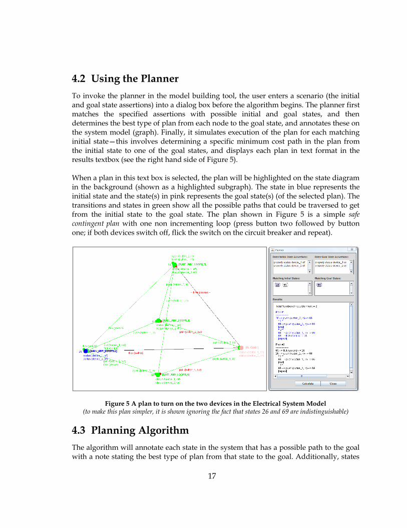
To invoke the planner in the model building tool, the user enters a scenario (the initial and goal state assertions) into a dialog box before the algorithm begins. The planner first matches the specified assertions with possible initial and goal states, and then determines the best type of plan from each node to the goal state, and annotates these on the system model (graph). Finally, it simulates execution of the plan for each matching initial state—this involves determining a specific minimum cost path in the plan from the initial state to one of the goal states, and displays each plan in text format in the results textbox (see the right hand side of Figure 5). When a plan in this text box is selected, the plan will be highlighted on the state diagram in the background (shown as a highlighted subgraph). The state in blue represents the initial state and the state(s) in pink represents the goal state(s) (of the selected plan). The transitions and states in green show all the possible paths that could be traversed to get from the initial state to the goal state. The plan shown in Figure 5 is a simple safe contingent plan with one non incrementing loop (press button two followed by button one; if both devices switch off, flick the switch on the circuit breaker and repeat).

Figure 5 A plan to turn on the two devices in the Electrical System Model (to make this plan simpler, it is shown ignoring the fact that states 26 and 69 are indistinguishable)

4.3 Planning Algorithm

The algorithm will annotate each state in the system that has a possible path to the goal with a note stating the best type of plan from that state to the goal. Additionally, states

18

will be annotated with the minimum number of actions that need to be carried out to get to a goal from that state as described in Section 4.1. These annotations make it fairly easy to visualize all possible plans by looking at the system graph (which provides a nice way for us to ensure the planner is producing reasonably intelligent plans), and they could potentially be stored with the models for reuse at a fairly minimal additional memory cost, if plans are carried out often in a real system. Finally, the execution of a plan will be simulated by following a path through the graph that moves to states that are annotated with a plan type that is better than the plan type of the current state, until a goal state is reached (this plan will be displayed in the results box).

4.3.1 A Simplistic Algorithm

A simplistic algorithm would perform a depth first traversal of the graph from each initial state, stopping when it reaches a goal state (no-loop), a dead end (none), or a node that loops back (loop). The values from these nodes could then be propagated back. Where an ambiguous action is found, the worst value from each possible outcome would be propagated. Where there is a choice of actions, the value of the best action would be propagated.

Figure 6 A simplified system where state 1 relies on state 3’s value, and vice-versa (the dotted blue lines are included to identify ambiguous actions)

Unfortunately, this procedure breaks down because of loops. To demonstrate, consider the case shown in Figure 6 above. There is an ambiguous action out of state 1 that either leads to state 2 (from which there is a path to state 4 [the goal] that involves a loop back to state 1) or to state 5 (which is a dead end), meaning the best plan from state 1 to a goal will be unsafe (as there is always a chance it may arrive at state 5). If we simply perform a depth first traversal from state 1, and propagate back values, then state 4 would be

1

5 2

3

4

action (one)

action (two)

action (three)

19

assigned no-loop, state 3 would be assigned the worst of no-loop and loop (which is loop), and state 2 would be assigned loop. Finally, state 5 would be assigned none and state 1 would be assigned unsafe. It is, however, clearly untrue that state 3 has a safe path to the goal involving a loop since the only plan from state 3 to the goal is in fact unsafe. It is not possible to determine the value of state 3 until all other paths out of state 1 have been evaluated, and it is not possible to determine the value of state 1 until state 3 has been evaluated. A simple solution would be to find all ―paths‖ to a goal. Even without loops, however, a depth first traversal of all paths to a goal may be exponential in the number of states, which would be intractable for large models. Therefore, a more complex algorithm is required.

4.3.2 Algorithm Overview

This section describes the planning algorithm with two simplifications: it constructs safe plans with no loops, safe plans with loops (whether they are incrementing loops or not), and unsafe plans, but ignores incrementing actions and assumes that all states are distinguishable. Sections 4.3.6 and 4.3.7 will address these simplifications. The algorithm will generate a plan from each distinguishable initial state to a set of possible goal states. Conceptually, this works as described below. Note the appendix provides a pseudo-code version of the algorithm which gives a more detailed specification of how the algorithm works. To begin, a depth first traversal is performed from the initial state throughout the system graph, stopping whenever an already visited or goal state is encountered. During this traversal, each node is labeled with an expression specifying the cost of the node as follows:

A goal state cost = [no-loop/0]

A state with no actions cost = [none]

A state with multiple actions (a & b) gets the best cost of cost = best(a,b)+1 its actions note the +1 corresponds to the cost of performing the action

An ambiguous action leading to states x & y contributes cost = worst(x,y) For example, state 1 in Figure 7 (which has ambiguous action one that goes to states 1 and 2, as well as action two that goes to state 3 and action three that goes to state 4) would be assigned the expression:

cost = best(worst(s1,s2),s3,s4)+1. If states 2 and 4 were goal states, then state 1 would be assigned the expression:

cost = best(worst(s1,[no-loop/0]),s3,[no-loop/0])+1.

20

Figure 7 A state with one ambiguous and two unambiguous actions

Note that, with the exception of goal states, any states that cannot be reached by a path from the initial state (or states that can only be reached by a path from the initial state that goes through a goal state) will be removed from the plan at this point. All goal states and dead ends will have an expression that contains no variables (a ―grounded cost‖). The next step is to perform a post-order depth first traversal to evaluate state expressions: values are propagated back from the leaves of the traversal (goal states, dead ends, or states whose value depends only on states that are all already on the traversed path) and substituted into the state expressions of their neighboring nodes. Once all states that a node depends on have been traversed, its expression is evaluated as much as possible. When a state’s expression includes a reference to the state itself, it substitutes in an intermediary value, at-least-loop, and evaluates. At any point in the traversal, if a state is given a grounded value (its expression is completely evaluated), this is propagated to any expression that contains a reference to this state and that expression is then further evaluated. Finally, the algorithm prunes states that have no paths to the goal (a value of none), except those that are directly connected to a state which has an unsafe value (such as state 5 in the example provided in Section 4.3.4, which is directly connected to state 1). Lemma: If a state’s expression remains dependent on some other state (because this other state was traversed through earlier), then there is definitely a path from this earlier state to the one whose expression we are evaluating (if there wasn’t, the earlier state would have been able to evaluate to a grounded value). The state’s expression will be expressed only in terms of states that have been travelled through on the way to it, and grounded costs. Thus, we know that as we propagate expressions back during the traversal, all state values will eventually be substituted for at-least-loop values (as we will step back

2

3 4

action (three)

1

action (one)

action (two)

21

through each corresponding state during the post-order traversal). When we return to the first state in the traversal, its expression must be expressed only in terms of grounded costs (there are no earlier states in the traversal) and so will definitely evaluate to a grounded value itself. This new value will then be propagated to any states that contain a reference to this first state. Now the second state in the traversal could only have been expressed in terms of the first state and grounded values, and thus it is guaranteed to obtain a grounded value after the first state’s value is substituted into its expression; the second state’s grounded value will then be propagated forward, and so on until all states have grounded expressions. The algorithm is guaranteed to terminate.

4.3.3 Evaluating Expressions

The key steps in evaluating an expression are evaluating worst and best functions. Other than several exceptions, when evaluating functions, the value of a worst function will be the worst type of plan in its arguments according to the following ordering, and the value a best function will be the best type of plan according to the following ordering (from best to worst):

[no-loop/0] > [no-loop/1] > … > [loop/1] > [loop/2] > … > [unsafe-or-at-least-loop] > [at-least-loop] > [unsafe] > [none]

Note that the no-loop and loop plan types are augmented with a number which represents the length of the plan since a shorter plan is always better than a longer plan of the same type. The exceptions mentioned above are used to determine where plans involving loops or plans that are unsafe occur. Table 2 gives a complete definition of the worst function, and Table 3 gives a complete definition of the best function. In addition to the details provided in the tables below, the following rules apply.

If a state’s expression is fully evaluated to the value [at-least-loop], its actual cost will be set to [none], since this means the state only has paths that loop back to itself (and there are no possible paths from it that lead to the goal). Similarly, if the final value is [unsafe-or-at-least-loop], the state’s actual cost will be set to [unsafe].

The +1 is only relevant to plans of type [no-loop] or [loop] (in which case the value is added to the count of the number of actions). Other types of plans simply ignore the added constant.

Note that both functions are:

Commutative worst(x,y) = worst(y,x) Associative worst(worst(x,y),z) = worst(x,worst(y,z)) = worst(x,y,z).

22

EVALUATING WORST EXPRESSIONS

worst(x,y) = x if x ≥ y given the ordering above = y if y ≥ x given the ordering above

except that:

worst([none],x) = [unsafe] if x is > at-least-loop or is unsafe Here we detect an unsafe plan as one transition out of an ambiguous action leads to a dead end. Note we can convert worst([none],[at-least-loop]) into none as it acts the same way as the value [at-least-unsafe] would.

worst([at-least-loop],[unsafe-or-at-least-loop]) = [unsafe-or-at-least-loop] There is definitely an unsafe path to the goal we can get to eventually, but we can still choose to loop back if preferred (see the description of unsafe-or-at-least-loop in Table 3)

worst([at-least-loop],x) = [loop/n] if x is [loop/n] or [no-loop/n] Here we detect a loop. One transition leads to a path to the goal, and the other leads to a path that loops back.

worst([unsafe-or-at-least-loop],x) = [loop/n] if x is [loop/n] or [no-loop/n] Here we detect a loop. One transition leads to a path to the goal, and the other can lead to a path that loops back.

worst ([loop/n],[loop/m]) = [loop/min(n,m)] We take the best case minimum path cost to exit a loop.

Table 2 The initial definition of the worst expression

EVALUATING BEST EXPRESSIONS

best(x,y)+1 = x+1 if x ≤ y given the ordering above = y+1 if y ≤ x given the ordering above

except that:

best([at-least-loop],[unsafe])+1 = [unsafe-or-at-least-loop] This case is needed because an at-least-loop value can be part of a loop plan which is better than an unsafe plan. If no such plan exists, however, at-least-loop will evaluate to none which is worse than an unsafe plan.

Table 3 The initial definition of the best expression

4.3.4 An example of the Algorithm in progress

A simple example of the algorithm applied to the system shown in Figure 8 is given below (note this is identical to the example used in Section 4.3.1). Assume state 1 is the initial state and state 4 is the goal state. Note that all states are reachable from state 1. The algorithm begins by assigning expressions to each state:

cost(s1) = worst(s2,s5)+1 cost(s2) = s3+1 cost(s3) = worst(s1,[no-loop/0])+1 cost(s4) = 0 cost(s5) = [none] (as there are no actions whatsoever out of state 5)

23

Figure 8 A simple example system

The algorithm will begin a traversal from state 1. State 1 will contact states 2 and 5 to get their updated cost values. State 5 will immediately return the grounded value [none], while state 2 will need to first contact state 3. State 3 does not need to contact state 1 as state 1 has already been visited in this traversal, and so can immediately return its cost to state 2 as is. State 2’s expression will then be updated as follows:

cost(s2) = s3+1 = worst(s1,[no-loop/0])+1+1 = worst(s1,[no-loop/0])+2 After receiving values from both states 2 and 5, state 1’s expression will then be updated and evaluated (at-least-loop will be substituted in for s1):

cost(s1) = worst(s2,s5)+1 = worst(worst(s1,[no-loop/0])+2,none)+1 = worst(worst([at-least-loop],[no-loop/0])+2,[none])+1 = worst([loop/2],[none])+1 = [unsafe] Now that state 1 has a grounded value, this will be updated in all states that rely on it; state 3 will become:

cost(s3) = worst(s1,[no loop/0])+1 = worst([unsafe],[no loop/0])+1 = [unsafe] Likewise, state 2 will be updated:

cost(s2) = worst(s1,[no-loop/0])+2 = worst([unsafe],[no-loop/0])+2 = [unsafe] And now that all states have a definite cost, the algorithm is complete. The final plan produced by the test program is shown below in Figure 9.

Note that this system does contain a loop (as can be inferred from the [repeat] command in the plan execution). The best type of plan from each state, however, is unsafe; since unsafe plans are considered worse than safe loop plans, the loop is effectively overridden by the ―worse‖ unsafe value.

1

5 2

3

4

action (one)

action (one)

action (one)

24

Figure 9 A plan produced in the example system

4.3.5 Complexity Issues

Note that for efficiency reasons, it is not enough to just update a state’s value in terms of succeeding states and immediately pass (propagate) that value back (as we did in the example). When multiple states are visited from multiple different paths, they would need to be expressed in terms of different preceding states each time. If this occurs repeatedly (as it will in non trivial systems), the expressions describing the value of a state become exponentially long. As an example, consider a fully connected graph where four states are all connected as follows (ignore goal states for now).

cost(s1) = best(s2,s3,s4)+1 cost(s2) = worst(s1,s3,s4)+1 cost(s3) = best(s1,s2,s4)+1 cost(s4) = worst(s1,s2,s3)+1 We begin traversing the graph from state 1. The last state visited (s4) will pass back its expression unchanged (that is, cost(s4) = worst(s1,s2,s3)+1). The preceding state will then set its expression to:

cost(s3) = best(s1,s2,s4)+1 = best(s1,s2,worst(s1,s2,s3)+1)+1 = best(s1,s2,worst(s1,s2,[at-least-loop/0])+1)+1 After this value is propagated back, the next preceding state will update its value:

cost(s2) = worst(s1,s3,s4)+1 = worst(s1,best(s1,s2,worst(s1,s2,[at-least-loop,0])+1)+1,worst(s1,s2,s3)+1)+1 = worst(s1,best(s1,s2,worst(s1,s2,[at-least-loop,0])+1)+1,worst(s1,s2,

best(s1,s2,worst(s1,s2,[at-least-loop,0])+1)+1)+1)+1

25

Clearly, if this process continues, expressions may become extremely long before they can be properly evaluated. One alternative would be to always propagate back temporary values and re-evaluate expressions for each state based on a specific path to that state. Only when a state obtains a grounded (definite) value would you update states’ actual values. This would be a small improvement on the above method. It would, however, still have exponential complexity as all possible paths from each state would need to be traversed. Two solutions were devised to complete the algorithm in polynomial time, both of

which operate in O(n·e) ≈ O(n3). The most straightforward method involves storing a map of expressions for each other state at each state. This way we only need to traverse each edge once but have evaluation and propagation costs which are O(n3). An alternative approach is to calculate temporary values once and store them along with an index representing the earliest state the expression refers back to in the order states were traversed. This index can be used to aid in evaluating values. The complexity is still O(n3) as each edge may need to be traversed up to n times. The appendix provides pseudo-code which shows how each algorithm works.

4.3.6 Dealing with Indistinguishable States

Models with indistinguishable states can cause the planner to suggest plans that are impossible to actually execute in practice. For example, consider Figure 10 below.

Figure 10 An invalid plan due to indistinguishable states

When the planner ignores indistinguishable states it may present a plan like the one shown above. The problem with this plan, however, is that it requires that the agent executing it be able to determine which state they are in (s2 or s3) after performing

action(one) from state 1 (and then to perform a different action depending on which state they happen to be in). As these states are indistinguishable, the agent won’t be able to make this distinction and so won’t be able to carry out the plan as it is shown in the diagram above.

26

There are several important observations we can make with regards to indistinguishable states. For two states to be indistinguishable, they must have not only identical properties observable in each state, but also have actions that are possible in both states but lead to different states—if they didn’t, then the states would be identical rather than just indistinguishable and wouldn’t have been separated by the learning agent. If one state has an action that the other does not, we assume the model is not complete and that the missing action has not yet been observed. As we have no idea what might happen if we perform the action in this state, we make the pessimistic assumption that performing the action may lead to a dead end (to a state with cost [none]). An alternative optimistic assumption would be to assume performing the action has no effect (thus the action could be used to infer which state the agent is in). More information about incomplete models is provided in the discussion in Section 5.3.4. There are two cases where a planner can run into problems due to indistinguishable states. The first (as shown in Figure 10 above) is when the plan goes through an ambiguous action that leads to two or more indistinguishable states (possibly several distinguishable states as well). When executing the plan, the agent can’t determine which state they have arrived at, and so the plan will have to be adjusted to take account of this. The second is when the agent’s initial observations (which are used to determine the initial state) match multiple indistinguishable states. To take account of indistinguishable states, the planner performs a preprocessing step. All indistinguishable states where the agent might not be able to determine which state it is in are converted into states where the agent does know exactly which state it is in. A state is created to represent a combination of states for each set of indistinguishable states that the agent may arrive at and not know which one they are actually in. The old indistinguishable states are retained; since they may be accessible via a non ambiguous action such that the agent would know they are in the state. After the preprocessing is completed, all nodes in the graph will represent a state such that the agent will always be able to determine exactly which node (state or combination of states) that it is in. This means the algorithm can be run unchanged on the new model and produce valid plans even in the presence of indistinguishable states. The planner achieves this by doing the following. The first time a model is used (after any changes), the planner will check each action in the graph. Where an ambiguous action that leads to two or more indistinguishable states is found, the planner will generate a new state. The new state will combine the corresponding actions out of each of the indistinguishable states into new ambiguous actions which can lead to any of the possible successor states that the given action may have lead to from each of the states being combined. The original ambiguous action leading to this set of indistinguishable states will be removed, and replaced with an action that leads directly to this new state. Where there are distinguishable states reachable via the same ambiguous action, the links to distinguishable states will remain unchanged.

27

Additionally, before any plan is generated, the planner will check to see if there are multiple indistinguishable states that match the list of the agent’s initial observations. If so, a similar approach to above will be taken: a new state will be generated that is a combination of the indistinguishable initial states. The planner will then compute a plan to a goal state from this newly generated initial state instead of from each indistinguishable state. Note that the new state may result in new ambiguous actions that lead to indistinguishable states, so the planner must also check each edge that it adds.

Figure 11 A valid plan taking into account indistinguishable states

Returning to the earlier example, Figure 11 shows how the planner would deal with this model when it takes into account the indistinguishable states. State 8 is generated, made from states 2 and 3. The corresponding best plan from the initial state is [unsafe]. This is

clearly accurate: the agent will have to choose action(one) or action(two), either of

which could lead to the dead_end state depending on which of states 2 or 3 the agent

actually arrives at after performing action(one) from state 1. Note that in this example, states 2 and 3 become redundant—there is no way an agent could ever arrive at state 2 or 3 and know that they are in that state. There are many scenarios, however, where an agent may or may not know which specific state they are in depending on which state they have come from (and what action they have just performed). Consider the corrected Fill a Sink model mentioned earlier. A small section of the model after the required indistinguishable states have been generated is shown below in Figure 12 (a large number of non relevant states have been removed). If the agent begins in state 72 (a combination of states 2, 59 and 60), pulling the plug out will lead it to state 18, 20, or 13 (the water level is decreasing, steady, or rising). If the agent then pushes the plug back in (from any of these states), it will know which specific state it is now in (2, 59 or 60).

28

Note that it is possible for the agent to arrive at state 76. If the agent gets to the state where the sink is empty, and the tap is partially rotated, then putting the plug in will move it to state 76 (the flow out the tap could be less than or equal to the flow out the plughole, but not greater). This transition is not shown in the diagram below—to make it readable, only a small section of the complete model is shown. States that the agent could never arrive at (such as a combination of states 59 and 60) won’t be generated.

Figure 12 A section of the Fill a Sink model with generated indistinguishable states

A significant benefit to the way indistinguishable states are handled is that the enhanced models can be stored for future use. The first preprocessing step only ever needs to be performed once per model (or could be computed every time the model is changed). The second preprocessing step would need to be carried out every time an agent wants to perform a new plan from a new set of indistinguishable initial states. The newly generated state could be stored or removed (or could depend on how often that particular plan is carried out—regardless, it takes minimal effort to generate just one new state). This is discussed further in the discussion in Section 5.3.3.

4.3.7 Detecting Incrementing (or Decrementing) Loops

As stated earlier, a loop that involves an incrementing action (denoted an incrementing loop) means that when one of the actions that initiates the loop is taken, if the undesired transition occurs (and leads us down a loop path), progress is made towards having the desired transition occur next time around the loop. For example, ―keep turning the tap until it reaches its maximum value‖. Figure 13 shows how this kind of standard incrementing loop is represented.

29

Figure 13 A standard incrementing loop

The progress made in incrementing loops ensures that eventually the agent will get out of the loop. Incrementing loops, therefore, can be considered categorically better than non incrementing loops, where we have no such guarantees (we might get stuck in a non incrementing loop forever). This adds a considerable amount of expressiveness to the system. An incrementing loop has to be detected by working out if there is an action in a loop that contains an increment that raises (or lowers) the value of some property, specifically a property that reaches a higher (or lower) value/range in a state that is reached via an ambiguous action that is an entry/exit to the loop. Before going into more detail, there are a few important observations to make with regards to incrementing loops that simplify what would otherwise be quite a complex analysis. First, any action that includes an increment must either always move to a new state with a new value for the incremented property, or else the action must be an ambiguous action. To understand why this is true, consider what an increment on an action means. If an action increments some property, then repeating the action enough times means the property must move to a higher value/range in which case the system must move to a different state. If the next value/range is not reached immediately, then performing the action will sometimes result in the same state and sometimes move to a new state, and therefore must be ambiguous. Note that it would be possible for an action to increase a property in an asymptotic manner, in which case the above observation would not hold. Actions that increment a property asymptotically do not, however, provide a guarantee that we will progress towards exiting a loop (where an exit exists that has a property in a higher range). Thus, these kinds of actions are simply ignored by the planner when it detects incrementing loops. A standard incrementing loop was shown in Figure 13. Note that in that figure, state 2 (the state succeeding the ambiguous action) has a higher value for the rotation property than the state preceding the action. If actions only affect one property value at a time, then it will always be the case that any states succeeding an ambiguous action with an increment will be in a higher (or lower) range (except the state that initiates the action). The end of this section discusses how we can attempt to detect incrementing loops when this is not the case.

2 1

rotate (tap, right) [ + rotation (tap) ]

rotation (tap, some) rotation (tap, max)

30

For now, we can infer from the assumption above that states succeeding an ambiguous action with an increment will always be in a higher (or lower) range. Thus, any path leading from any of these succeeding states back to the preceding state must include an action that increments the property in the opposite direction (decrements it) as the property would need to go back down a range. This means that when looking for incrementing loops, we only need to inspect ambiguous actions that involve edges that loop back to the same state or are on a path directly to a goal. It also means we do not need to be concerned about suggesting a specific path to get to an action that contains an increment just so that a loop becomes incrementing (if an action with an increment exists, it will be found on the ambiguous action that acts as an entry/exit to the loop itself). Additionally, inner incrementing loops cannot exist (as inner loops stem from edges that (a) are not on a path to a goal and (b) do not loop directly back to the same state). It’s worth noting that given the properties discussed above, the planner still needs actions that include increments to be annotated as such; they cannot simply be inferred from the models. Consider the case of a button that will either do nothing or turn the tap to max flow as compared to a rotatable handle that increments a tap’s flow—the graph structures would be identical apart from the increment annotation. The process used to detect incrementing loops is described below. Initially, when labeling states with expressions, we note cases where a state has an ambiguous action with one transition that loops back to itself and involves an increment. The increment must increment (or decrement) the property that moves to a higher (or lower) range via all other transitions that are part of the same ambiguous action. Note that we use * to mark a value that has associated increments (satisfying the conditions above). All the information needed to evaluate whether or not a loop is an incrementing loop is available at the state where the self loop with an increment occurs (the information does not need to be propagated around at all). Whenever a cost(z) = worst(z*,x) = worst([at-least-loop]*,x) function is being evaluated, if x is [no-loop], or incrementing-loop (denoted [inc-loop]), then the function will evaluate to [inc-loop]. A more detailed explanation of how expressions are evaluated when incorporating this kind of information about incrementing loops is provided below.

31

We add the inc-loop value (as mentioned above) to the list of possible values for states. As before, other than several exceptions, when evaluating functions, a worst function will choose the worst type of plan in the list and a best function will choose the best type of plan, where plan types are ordered from best to worst as follows: [no-loop/0] > [no-loop/1] > … > [inc-loop/1] > [inc-loop/2] > … > [loop/1] > [loop/2] > … > (as before).

The only new exceptions are shown below:

additional exceptions for the worst expression:

worst([at-least-loop]*,x) = [loop/n] if x is [loop/n] = [inc-loop/n] if x is [no-loop/n] or [inc-loop/n]

Here we may detect an incrementing loop if: one transition leads to a goal via a no-loop or inc-loop path, and the other is a self loop with an increment.

worst ([inc-loop/n],[inc-loop/m]) = [inc-loop/min(n,m)] As with standard loops, we take the best case minimum path cost to exit an incrementing loop.

Table 4 Extra details for the worst expression to detect simple incrementing loops

Earlier, we noted that it will be more difficult to evaluate incrementing loops if we consider that an action may change multiple values. Figure 14 gives an example of this. In this example, turning the tap not only increases the flow of water out of it, but also has the possibility of breaking the tap.

Figure 14 An incrementing loop that affects two values

Up until now we have been able to treat all loops in the same way. Most importantly, a loop inside a loop could be collapsed into just one loop value (we wouldn’t need to pay special attention to inner loops). Now, however, ―inner‖ loops (that don’t lead directly to a goal via any path) may or may not be incrementing. This means that after detecting a path back to an already visited node, we cannot simply insert the at-least-loop value.

rotation (tap, some)

working (tap, no)

3

1

rotation (tap, some)

working (tap, yes)

rotation (tap, max)

working (tap, yes)

rotation (tap, max)

working (tap, no)

4

fix (tap)

2

fix (tap)

rotate (tap, right) [ + rotation (tap) ]

32

Consider Figure 15 (an extension of Figure 14) below which has a built in ―fix-knob‖ which can be turned in order to fix the tap. If this system is evaluated beginning from state 1, then state 2 will be given the expression worst([at-least-loop],s1). When state 1’s expression is evaluated, [at-least-loop] would be substituted for s1, and the evaluation would ignore the fact that there is an inner loop at state 2.

Figure 15 An inner incrementing loop

To detect these kinds of incrementing loops, we record two indices on all at-least-loop values denoting the specific ―earliest‖ state they link back to (these indices are described in more detail in the following paragraph). Additionally, all actions that contain increments are annotated with a reference (*) that specifies which transition(s) the

increment moves towards (for example, in Figure 15 above, the action rotate(fix-knob,

left) from state 2 moves toward the transition from state 2 to state 1 eventually occurring). In addition, we know the index of the state each expression belongs to.

When evaluating a worst expression that contains all at-least-loop values, the result will be at-least-loop-x-y, where:

x is the index of the latest state (in the order states were visited in the traversal) reached by one of the specified transition(s) (that the increment moves towards). If the at-least-loop values do not contain such a reference, the value will be indexed by the latest state that any of the transitions lead to (in this case we don’t have an inner loop, but simply a loop with multiple exits); and

y is the index of earliest state that the loop could go back to as a non incrementing loop

rotation (tap, some)

rotation (fix-knob, some)

3

1

rotation (tap, some)

rotation (fix-knob, min)

rotation (tap, max)

rotation (fix-knob, min)

rotation (tap, max)

rotation (fix-knob, some)

rotate (fix-knob, left) [ - rotation (fix-knob) ]

rotate (fix-knob, left) [ - rotation (fix-knob) ]

2

rotate (tap, right) [ + rotation (tap) ]

4

33

When a loop back to a traversed node is detected and we substitute in the at-least-loop value, both x and y will be set to the index of node that the transition leads to. The indices will be updated when expressions are evaluated (see Table 5 and Table 6 below). As an example, an expression might evaluate to [at-least-loop-2-1]. This means 2 is the index of the earliest state the loop can get back to as an incrementing loop, and 1 is the index of the earliest state the loop can get back to as a non incrementing loop. The former index (the x index) specifies that states with an earlier index than 2 cannot use this path to evaluate to inc-loop as getting back to such a state requires going through an inner loop that is not incrementing. Additionally, we need to introduce the value at-most-loop, to represent the case where a node has one path to a goal and another that loops back to an earlier node—the loop back may or may not be able to be used as the loop part of an incrementing loop, but there is at least a loop plan to the goal from this state. These values are indexed with x as above, the earliest state they can go back to either directly or via an incrementing inner loop. They don’t need to also be indexed with y, the earliest state they could go back to via a non-incrementing loop, as at-most-loop means we have already found a path to a goal that is a non-incrementing loop. When evaluating an expression for a given state, if the values at-least-loop or at-most-loop are present and their x index comes after the given state’s index, they are effectively treated as at-least-non-inc-loop and loop respectively. If an at-least-loop value is present and its y index comes after the given state’s index, it is treated as none (as this would mean we have a loop back to a node that comes after the current node). This procedure is formalized in Tables 5 and 6 below. We add at-most-loop values to the ordering as shown below. (as before) > [inc-loop/1] > [inc-loop/2] > … > [at-most-loop/1] > [at-most-loop/2] > … > [loop/1] > [loop/2] > (as before).

With the introduction of the new intermediary value at-most-loop and the index values, there are now a range of special cases to consider when evaluating expressions, both in terms of exceptions to the ordering rule, and how to deal with indices. These are shown in Table 5 and Table 6. For all the special cases shown below, we use ai, bi, ... to refer to the indices of states a, b, ... respectively. Also recall that for any value [at-least-loop-yi-xi] state y must have came

before state x in the traversal (or x = y). Hence, xi ≤ yi.

Earlier, we noted that if a state’s expression evaluates to the grounded value at-least-loop then its actual cost will be set to none, or if it evaluates to unsafe-or-at-least-loop, its actual cost will be set to unsafe. Additionally now, if a state’s expression evaluates to the grounded value [at-most-loop/n], then its actual cost will be set to [loop/n].

34

additional special cases for the worst expression:

worst([at-least-loop-bi-ai]*, [no-loop/n]* or [inc-loop/n]*)

= [inc-loop/n] if * denotes the transition leading to the no/inc-loop

path and the index of the state being evaluated is ≥ bi

= [at-most-loop-bi/n] if above fails, and the index of the state being

evaluated is ≥ ai

= [unsafe] otherwise (the index of the state being evaluated is < ai) An ambiguous action where one transition leads to a path that loops back but potentially via a non incrementing inner loop (if looping back beyond state b), and the other leads to a path that gets to the goal via a no-loop or inc-loop path. To evaluate to inc-loop, not only does the * need to reference the correct transition in this loop (that is, the one leading to

the no-loop or inc-loop path), but additionally the index of the state being evaluated must be ≥ bi

worst([at-most-loop-bi/m]*, [no-loop/n]* or [inc-loop/n]*)

= [inc-loop/n] if * denotes the transition leading to the no/inc-loop

path and the index of the state being evaluated is ≥ bi

= [at-most-loop-bi/m] otherwise Since at-most-loop means we can follow a path that loops back to state b (or later), we may be able to combine this with a no-loop or inc-loop path to find a valid incrementing loop. If not, we definitely at least have a normal loop plan.

worst([at-least-loop-bi-ai]*, [at-least-loop-di-ci]*)

= [at-least-loop-earliest(bi,di)-earliest(ai,ci)] if * denotes the transition leading to the path with earliest(bi,di) and

the index of the state being evaluated is ≥ latest(bi,di) = [at-least-loop-latest(bi,di)-earliest(ai,ci)] otherwise

A path that loops back to two different earlier states. Each loop back has an index of the earliest node it can loop back to incrementally, and the earliest node it can loop back to non-incrementally. The expression will evaluate to at-least-loop, and the indices will be decided as follows: - the y index (representing the earliest non-incremental loop back) will be the earliest of the y indices of each of the two separate looping paths - the x index (representing the earliest incremental loop back) will be the latest of the x indices of each of the two separate looping paths, unless * references the correct transition (that is, the one leading to the path with the earlier x index) and

additionally the index of the state being evaluated is ≥ the latest x index

worst([at-most-loop-bi/n]*, [at-least-loop-di-ci]*)

= [at-most-loop-earliest(bi,di)/n] if * denotes the transition leading to the path with earliest(bi,di) and

the index of the state being evaluated is ≥ latest(bi,di) = [at-most-loop-latest(bi,di)/n] otherwise

Similar to above but considering an at-most-loop with an at-least-loop

worst([at-most-loop-bi/n]*, [at-most-loop-di /m]*)

= [at-most-loop-earliest(bi,di)/min(m,n)] if * denotes the transition leading to the path with earliest(bi,di) and

the index of the state being evaluated is ≥ latest(bi,di) = [at-most-loop-latest(bi,di)/min(m,n)] otherwise

Similar to above but considering two at-most-loops.

Table 5 Special cases for the worst expression to detect complex incrementing loops

Note the value unsafe-or-at-least-loop will be annotated with indices in exactly the same way as at-least-loop values are and is treated similarly. Additionally, we now need to annotate actions (rather than just states) with costs, so that the planning agent is able to correctly decide which action it should take when executing a plan. This is a simple extension to the algorithm—the cost of an action can be derived directly from the expressions as they are evaluated; we don’t show these annotations on the diagrams as the diagrams would become too cluttered, but the agent does look at the action costs when executing plans.

35

additional special cases for the best expression:

best([loop/n], [at-least-loop-bi-ai])+1

= [at-most-loop-bi/n+1] if the index of the state being evaluated

is ≥ bi = [loop/n+1] otherwise

A choice between a path that gets to the goal via a non incrementing loop and a path that loops back to an earlier node

best([at-least-loop-bi-ai], [at-least-loop-di-ci])+1

= [at-least-loop-earliest(bi,di)-earliest(ai,ci)]

We can choose the path with the earliest index to suit us

best([at-most-loop-bi/n]*, [at-least-loop-di-ci]*)+1

= [at-most-loop-earliest(bi,di)/n+1]

Similar to above but considering an at-most-loop with an at-least-loop

best([at-most-loop-bi/n]*, [at-most-loop-di /m]*)+1

= [at-most-loop-earliest(bi,di)/min(m,n)+1]

Similar to above but considering two at-most-loops.

Table 6 Special cases for the best expression to detect complex incrementing loops

One minor issue with this analysis of incrementing loops is that we will consider loops where the value of a property oscillates between ranges / values as incrementing loops. Figure 16 shows what we mean by an oscillating loop (although this example is quite artificial). The value of the ―level‖ property will be incremented up and down in this loop. It would be possible, therefore, that the agent could become stuck in this loop forever (if the increments and decrements exactly offset each other over time).

Figure 16 A system with an oscillating loop

It is unlikely that the increments and decrements in an oscillating loop would perfectly offset each other. As future work, it may be worth extending the analysis to detect loops of this kind and report them to the planning agent in a different way than incrementing loops. There is one more case of incrementing loops that we have so far avoided: it may be possible for an ambiguous action to increment a property on some of its transitions and

2

1 action (inc) [ + property (level) ]

property (level, 3)

3

4

property (level, 1)

property (level, 2) property (level, 0) action (dec) [ - property (level) ]

36

not others. In such cases, it may still be possible for an incrementing loop to occur at this action, if an increment is picked up at a later point, as shown in Figure 17. Performing

action (one) may leave the agent either in state 1 or move it to state 3 where the ―level‖

property has changed to max (in either case, incrementing the level property), or it may cause the button to be turned off (without incrementing the level property).

Figure 17 An ambiguous action that contains an increment on some of its transitions

There is an incrementing loop through state 1, because the path from state 2 back to state

1 increments the same property that is incremented via all transitions involved in action

(one), other than the transition going from state 1 to state 2. This path that loops back

from state 2 includes an ambiguous action, action (two). Given the observations noted at the beginning of this section and ignoring asymptotic increments, it must always be the case that a path that loops back like this and contains the corresponding increment includes an ambiguous action. As such, there must be another exit to the loop via this ambiguous action. In Figure 17, the other exit to the loop is via state 2—our analysis will result in an incrementing loop being detected at this state. Therefore, in this case, it does not matter that the incrementing loop via the exit at state 1 is not detected (we only need to detect an incrementing loop at one of the exits of a loop and it will suffice for the whole loop). It may be possible for more complex cases of these kinds of incrementing loops to not be detected by our analysis, but it is unlikely (perhaps impossible) for such cases to occur in practice. Attempting to analyze loops of this kind would make things significantly more difficult as it would require propagating incrementing values around the system. It may even require that the planning agent follows a specific path to get to a particular action that contains an increment, just so a loop becomes incrementing. This would undoubtedly mean an increase in the complexity of both detecting and also executing plans.

property (level, some)

property (button, off)

3

1

property (level, some)

property (button, on)

property (level, max)

property (button, on)

action (two) [ + property (level) ]

2

action (one) [ + property (level) ]

action (one) []

action (one) [ + property (level) ]

37

5 Discussion / Future Work

5.1 Choosing Optimal Paths

The planner is only able to produce plans in the context of the models that are provided by the learning agent. Due to the features (or lack of features) in these models, there are some limitations on the reasoning that can be implemented in the planner. The current algorithm selects the plan with the best worst case path to a goal. When there are loops involved, the best case path to get out of the loop is selected. These choices usually result in the production of plans that are similar to what a real person would come up with. There are, however, cases where the planner may make poor decisions about which paths to follow. Such cases are not common given the types of models we are attempting to make decisions in—that is, models describing the interaction of an agent with physical objects in a (simulated) 3D world—but aren’t overly rare either. A couple of key issues that can cause suboptimal plans to be produced are discussed below. The planner is likely to produce poor plans when faced with time passing actions (or other actions that require extra exertion to complete), as it has no way to decide ―how long‖ it may take to transition to another state or ―how difficult‖ an action is to perform. The Fill a Sink model is an example of this. Indeed, if an agent generates a plan to fill the sink (starting from an empty sink), the suggested plan will tell the agent to turn the tap to the right once, then wait until the sink fills up (it won’t tell the agent to continue turning the tap to reduce the time taken to fill the sink). This is a common issue in qualitative models (related to the discussion about bailing out water from an ocean-liner using a teaspoon in Section 2.2). It would be possible to improve the planner so that it can produce better plans in these cases by adding ―costs‖ to actions which could represent the approximate amount of time it will take for this action to occur. This is discussed further in Section 5.2 below (this would also aid in the addition of without delay annotations, see Section 5.3.6). There are, however, limitations to how the quantitative information can be added to a fundamentally qualitative model. Another common property of systems that can cause the planner to come up with suboptimal plans is the existence of ambiguous actions where the undesired transition has only a very low probability of occurring (maybe a one in a thousand chance). For example, when turning on a light, there is a very small chance the bulb will blow. If there were a ―more complex‖ way to achieve the goal of turning the light on, without the chance of blowing the bulb, the planner would most probably select this instead, as the possibility of the light bulb blowing results in an unsafe plan (or just a very high cost plan if the system includes information for replacing a blown bulb). Probabilities on actions are a possible way to improve plans in the face of these kinds of ambiguous actions. The effects of including probabilities into the models are discussed below.

38

5.2 Costs and Probabilities on Actions

For the reasons mentioned above, it may be desirable to have more detailed models that include both costs on actions (representing the time taken, and/or effort required), and probabilities on ambiguous actions (representing the chance of going down each possible transition). Annotating the models with these features would be the responsibility of the learning agent, and so is outside the scope of this project. It is worth considering, however, how the planner might be adapted to account for this information if it were ever added. Firstly, incorporating costs on actions into the plans produced would be a relatively simple task. Currently, we count the number of actions in the analysis, implicitly (or explicitly in the equations) assuming that each action has a cost of one. Using actual action costs instead of just one would be a trivial extension to the planning algorithm. Things get more interesting, however, when we consider the case of filling the sink. If the model is annotated correctly, then the cost (time taken) of moving to a full sink from a state in which the tap is rotated max should be significantly less than the cost of moving to a full sink when the tap is rotated only some. Additionally, the cost of rotating the tap itself should be trivial compared to either of these costs. When planning then, we would need to specifically distinguish between time passing transitions and transitions caused by actions. When waiting for time passing transitions to occur, the planner should look for actions that can progress the agent to a desired state quicker. This would mean the plan suggested to fill a sink would tell the agent to keep turning the tap until its rotated to max then wait until the sink fills up (note we can’t do this analysis in the current models, as there is no way to distinguish between different costs of different time passing events—we don’t know that it takes less time for the sink to fill up when the tap is rotated to its maximum). The inclusion of valid probabilities would present a rather difficult challenge for the learning agent, and may not make sense in a qualitative world. Probabilities would remove the need for the worst function; we could instead determine the value of each branch and take the product of these with the probabilities. Likewise, loops (and hence incrementing loops as well) would no longer need to be explicitly detected. The values of loops would be implicitly calculated in this process. The best (or minimum) function would remain, and unsafe states would still need to be considered (the value of unsafe states could be treated separately, or they could be detected and annotated in the same way they are now). It’s worth noting that a finite state automaton which includes probabilities is very similar to the models used by value iteration and similar algorithms. There is still a difference in that our models have features specifically relating to interaction with physical objects. Also, we would determine state values by solving a system of simultaneous equations as opposed to a recursive, more time-consuming technique.

39

5.3 Integration with the Learning Agent

A key consideration when implementing the planner was to ensure it will be able to be integrated with the learning agent, and with the physics engine used by the learning agent so we can see it carry out its plans in a 3D world. As such, the way models are stored in the planner has been implemented in a similar way to how models are represented by the learning agent. There are a range of other issues that need to be considered before a full integration could be completed. Some of these are considered below.

5.3.1 Efficiency (complexity) of the Algorithm

It’s clearly important that the algorithm runs in acceptable time if it is to be useful in practice. Learning of models is conducted iteratively as the agent performs actions (or time passes), and as such it is not such an issue for the learning algorithm. The planner, however, may need to produce an entire plan and the agent should know which actions to start taking fairly quickly. Both versions of the final algorithm used are O(n3) (time efficiency) both in the worst and average case. The pseudo-code for each algorithm is supplied in the Appendix. An overview of the worst case costs is given below. A worst case model would mean every state has an edge leading to every other state including to itself (note in our models, states may have multiple actions going between the same two states, so the cost could potentially be higher than this, but we assume that this does not happen enough to skew the calculations). The first version of the algorithm performs only one traversal, thus the worst case traversal cost is n2. The worst case evaluation cost is n2 for the first state

evaluated (have to evaluate up to n expressions of up to length n), and n·(n-i) for the ith

evaluation. In summation, this means a worst cost of 1/2·n·n·(n+1). Finally there is a cost

to propagate the values back; in the worst case this is 1/6·n·(n-1)·(2n-1). In total then, the

worst case cost is 1/2·n3+n2+1/6·n. The second version of the algorithm has an identical

total cost; the extra traversal cost is offset by the reduced propagation cost. In practice, the algorithm will run substantially faster, as any time we reach a state that is a goal state or leads only to a goal state, we can immediately update its value and propagate this value to any neighboring states. Additionally, the efficiency can be improved further by identifying expressions that can be immediately resolved without having to evaluate fully all neighboring states. For example, the expression best([no-loop,0],a,b,c) will always evaluate to [no-loop,0]; we don’t need to consider the values of states a, b and c.

40

Note the time taken to perform the pre-processing step for indistinguishable states, and the extra processing required to detect incrementing loops don’t have much of an effect on the overall efficiency of the algorithm. The running time of the planning algorithm can be further improved in a couple of ways as described in Sections 5.3.2 and 5.3.3 below.

5.3.2 Anytime (real-time) Algorithm

The algorithm should be able to run in real-time; that is, it should be able to return possible routes to a goal as they are found (even if they haven’t been fully evaluated yet), and return them as soon as they are found to the agent, then continue calculating routes and returning improved ones (adjusted depending on which state the agent has moved to since learning of the initial route). This would be done by adjusting the algorithm to keep a record of the path followed to get to a specific state during the depth first traversal. Where a plan is found to a goal, that goes through an ambiguous action, that leads to some states that have not been evaluated, the plan can be returned to the agent as an unsafe plan, which can begin executing the plan if it desires (until it gets to a node that has not yet been evaluated). Because the algorithm eventually determines the best type of plan from each node in a given system (that is on a possible path between the initial state and a goal state) to a goal state, any state that the agent may move to will be evaluated at some point.

5.3.3 Storage of Models

An interesting question this raises is whether or not the annotations placed on states in a system should be stored (for each possible set of goal states) along with the system in memory. If this information is stored, then repeating a plan will only take its execution time, O(x), where x is the number of edges in the plan. Holding annotations for each state for each set of goal states that an agent has produced a plan for in the past would, on the other hand, incur a large memory cost. A compromise may be to only store annotations for frequently used plans (and a number of the most recently generated plans so that we can determine which ones are frequently used). Note that two plans generated from different initial states to the same set of goal states will generate the same set of annotations (although potentially a different set of states in the system would actually be annotated). Thus, it is only for different goal states that different sets of annotations need to be stored.

41

5.3.4 Handling Incomplete Models

Up until now, the assumption has always been that the planner generates plans from a model that has been completely learned by the learning agent. It may be that some models have, for some reason, not been fully learned. In such systems, it will be impossible for the planner to always produce optimal plans. When the planner discovers it is impossible to get to a goal state in a particular system—

which will take at most e (≈ n2 in the worst case) steps—it would be possible to instead produce plans that get the agent to a state that is ―as close as possible‖ to the goal state, in terms of assertions that are true in these states. Ideally it would also be possible to infer actions that are likely to move the agent to a goal state from one of these states. For example, if performing a particular action changes the value of a property in a certain way somewhere in a system, it is likely performing the same action from another state will result in the same change to the same property value. This way the planner could potentially suggest actions that the agent should take to better learn the system; it would result in a much better integration between the learning and planning agents.

5.3.5 Extending to Multiple Systems

Perhaps the most important issue that would need to be taken into account before integrating the planner with the learning agent would be to determine the best way to plan tasks that span multiple system models. The algorithm will need to locate desired goal states which may span a set of possible systems (there may even be states that matching goal states in more than one system), and deal with transitioning between systems to get to a goal state in an efficient manner. If a naïve ―joining‖ of multiple systems was performed, the number of states would increase exponentially. We specifically want to avoid this happening. Instead the planner would need to match states that ―link‖ systems. The work done in implementing the preprocessing step for indistinguishable states would help here, as linking states are likely to be indistinguishable. The revised Fill a Sink model can, in fact, be split into multiple separate systems (systems for using the tap and using the plug independently). Two of these models, one corresponding to the system where the plug is always in and another to the system where the plug is always out are shown in Figure 18 and Figure 19 below.

42

Figure 18 The Fill a Sink subsystem with the plug in

Figure 19 The Fill a Sink subsystem with the plug out

43

These systems would provide a good way to evaluate the performance and benefits of a multiple system planning algorithm compared with the current algorithm which works on the larger single system. Note that state 9 in Figure 18 links to state 1 in Figure 19 via

the pull(plug, out) action (it could act as a linking state between the two models). Likewise, state 2 links with states 13, 18 and 20. State 3 corresponds to state 14, and so on.

5.3.6 Without Delay Annotations

Earlier, ―without delay‖ annotations were mentioned, which could be used to let an agent know that, when in a certain state, they must perform an action quickly to avoid a ―time passing‖ action occurring and taking them to an undesired state. Such annotations would be a simple addition to the algorithm. While executing the plan, the planner would simply need to identify states that contain a ―time passing‖ action that is not used, and insert a ―without delay‖ message at that point (note care would need to be taken when combining this with the cost on action changes proposed in Section 5.2). This information provides negligible benefit, however, as we would generally assume our planning agent would execute plans as quickly as possible.

5.4 Planning with Qualitative Differential Equations

The planning algorithm produced is coming up with plans based on qualitative differential equations (as discussed in Section 2.2). The models that the planner works on are generated directly from physical systems. The envisionment of a QDE is a graph that represents the possible qualitative behaviors of a system, and can be generated directly by repeatedly determining the possible successors of each state based on the QDE. Thus, to apply this planner to a QDE, we would simply need to generate the envisionment then apply the planning algorithm to that graph. Whether or not this would be useful in practice would be another interesting topic for future work.

44

6 Conclusion

The goal of this project was to develop a planning algorithm that uses a specific type of system model to come up with good contingent plans to take an agent from its initial state to a desired goal state. The system models used are able to be generated by a learning agent that learns in a virtual 3D environment; in these models, knowledge is represented using finite state automata, first-order logic, and qualitative physics. This report has presented four contributions of the project:

A set of models with specific properties were constructed, as well as a number of other models with which to test the planning algorithm.

A tool was built for constructing, editing, visualizing and storing the kinds of models used by the planner.

The key contribution was the completion of an implementation of the planning algorithm that is able to produce good plans (demonstrating a satisfactory level of intelligence) within any given system and handles ambiguous actions, loops, unsafe plans, indistinguishable states, and incrementing actions.

A calculus of qualitative plan values was also produced. The report has also identified several areas for possible future work, looking at how to extend the algorithm to handle more detailed information (costs and/or probabilities on actions). A range of issues surrounding the integration of the planner with the learning agent have been discussed, including a look at some of the key problems that may arise when combining multiple systems. It was also noted that the planning algorithm could be used to solve qualitative differential equations via envisionment.

45

7 Bibliography

1. Forbus, K. (1998). Qualitative physics: Past, present and future. In Exploring Artificial Intelligence, Morgan-Kaufmann.

2. Forbus, K. (1989). Introducing Actions Into Qualitative Simulation. In N. S. Sridharan, editeur, Proceedings of the Eleventh International Joint Conference on Artificial Intelligence, pages 1273-1278, San Mateo, California. Morgan Kaufmann.

3. Frean, M. (2009). Reinforcement Learning (by Value Functions). [Lecture Notes] Victoria University of Wellington.

4. Hinrichs, T., Nichols N. & Forbus, K. (2006). Using Qualitative Reasoning in Learning Strategy Games: A Preliminary Report. Qualitative Reasoning Group, Northwestern University.

5. Hinrichs, T. & Forbus, K. (2007). Analogical Learning in a Turn-Based Strategy Game. Qualitative Reasoning Group, Northwestern University.

6. Kuipers, B. Qualitative simulation. (2001). Encyclopedia of Physical Science and Technology, Third Edition, pages 287-300.

7. Kuipers, B. & Mugan, J. (2007). Learning to predict the effects of actions: synergy between rules and landmarks. In IEEE International Conference on Development and Learning (ICDL-07).

8. McDermott, D. (1998). PDDL - the planning domain definition language. 9. Russell, S. & Norvig, P. (2003). Artificial Intelligence: A Modern Approach, Second

Edition. Pearson Education Inc. 10. Tijms, H.C. (2003). A First Course in Stochastic Models. John Wiley & Sons Ltd.

46

8 Appendix

8.1 Algorithm Version One

This version of the algorithm involves storing a map at each state containing the expressions for each other state. As such, each state will only need to compute the value of each other state once. This version terminates after a single traversal of each edge in the model. The evaluation and propagation costs, however, result in the algorithm

running in O(n·e) ≈ O(n3). Note this version of the algorithm has been extended to include detection of incrementing loops. Starts up the algorithm by identifying initial and goal states, then generates any required indistinguishable states.

Then, for each initial states, the state expressions are initialised, each state’s value is calculated, and finally unused states are removed.

procedure: plan()

1. initialStates <- states that contain all specified intial state predicates

2. goalStates <- states that contain all specified goal state predicates

3.

4. generateIndistinguishableStates()

5. for each initialState in initialStates

6. initialize(initialState)

7. for each state in the model

8. if state does not have a grounded value

9. calculateValue(state)

10. highlightPlan()

Initialises the value of all states (recursively) to an expression (in terms of neighboring states).

procedure: initialize(state)

1. add state to list initialisedStates * additional information is included

2. here that specifies the incrementing

3. if state is a goal state value(s) that are on each transition

4. state.value <- [no-loop/0]

5. else if state has no actions

6. state.value <- [none]

7. else

8. for each action out of state

9. reachableStateVariables <- variables representing all states reachable via this action

10. if reachableStateVariables.size = 1 // ie: a distinct action

11. add expression “reachableStateVariable*” to tempValues // eg: s1

12. else if reachableStateVariables.size > 1 // ie: an ambiguous action

13. add expression “worst(<reachableStateVariables>*)” to tempValues // eg: worst(s2,s3,s4)

14. state.value <- expression “best(<tempValues>)+1” // eg: best(s1,worst(s2,s3,s4))+1

15.

16. for each uninitialised neighboringState reachable out of an action from this state

17. initialize(neighboringState)

47

Performs a post order depth first traversal to evaluate the value of all states (ie: begins running the core of the algorithm).

procedure: calculateValue(state) -> value

1. add state to the pathSoFar list of states that have been traversed through

2.

3. if state.value is not grounded

4. for each neighbState that has a corresponding variable in the state.tempValue expression

5. if neighbState has not yet been visited

6. value = calculateValue(neighbState)

7. for each entry in neighbState.map

8. state.map.put(entry.state,copy of entry.value)

9. state.map.put(neighbState,copy of value)

10.

11. return updateMap(state)

Performs an update to evaluate as many of the expressions in state’s map as possible.

If all values in state’s map become grounded, and all the variables in state’s own value expression are in state’s map, then state’s value

will be able to be fully evaluated (become grounded). It will then propagate its grounded value to all dependent nodes.

procedure: updateMap(state,pathSoFar) -> value

1. for each visitedState in pathSoFar (in order of last to first)

2. if visitedState that is in state.map

3. for each neighbState of visitedState that has a variable in visitedStatesValueInMap

4. if neighState is in state.map and map.get(neighbState) is grounded

5. cascadingUpdate(state.map,visitedState,neighbState,map.get(neighbState))

6. else if neighbState is in state.map and neighbState = visitedState

7. cascadingUpdate(state.map,visitedState,neighbState,[at-least-loop(index of visitedState)])

8. else if neighState = state

9. cascadingUpdate(state.map,visitedState,neighbState,[at-least-loop(index of state)])

10. cascadingUpdate(state.map,state,state, [at-least-loop(index of state)])

11.

12. if all states in map are now grounded & all neighbState vars in state.value are in map

13. for each neighbState in state.value

14. cascadingUpdate(state.value,neighbState,map.get(neighbState))

15. evaluateStateValue(state.value)

16. for each dependentState in the model // state’s that have this state as a neighbor

17. propogateUpdate(dependentState,state,state.value,pathSoFar)

18.

19. return state.value

1. substitute valueToBeSubstitutedForState for state in stateToBeUpdated’s value expression.

2. if stateToBeUpdated’s value becomes grounded, recursively cascade the new grounded value to all other values in map.

(note that valueToBeSubstitutedForState will be grounded when this function is invoked)

procedure: cascadingUpdate(map,stateToBeUpdated,state,valueToBeSubstitutedForState)

1. valueToBeUpdated = map.get(stateToBeUpdated)

2. for each stateVariable in valueToBeUpdated

3. if stateVariable = state

4. stateVariable.value <- valueToBeSubstitutedForState

5. evaluateStateValue(valueToBeUpdated)

6.

7. if valueToBeUpdated is now grounded

8. for each visitedState in map

9. visitedStatesValueInMap = map.get(visitedState)

10. cascadingUpdate(map,visitedStatesValueInMap,stateToBeUpdated,valueToBeUpdated)

48

Fully evaluates the value expression (which will not contain any references to other states when this method is called)

procedure: evaluateStateValue(value)

1. evaluate a value expression into a grounded value using the rules described in Tables 2-6

Propagates the update of a grounded value (value) for a state (stateToBeUpdated) throughout the graph

procedure: propogateUpdate(state,stateToBeUpdated,value,pathSoFar)

1. if state.value is not grounded

2. state.map.put(stateToBeUpdated,value)

3.

4. updateMap(state,pathSoFar)

POST-PROCESSING

Highlight all states that are involved in any possible plan from the initial state to a goal state.

procedure: highlightPlan()

1. for each state reachable via a traversal from the initial state to a goal state

2. if state.value is better than none

3. or state is reachable (via an ambiguous action) from another state whose value is unsafe

4. mark state as highlighted

PRE-PROCESSING

1. generate new states where an ambiguous action leads to two or more indistinguishable states

2. generate new states where two or more initial states are indistinguishable

procedure: generateIndistinguishableStates()

1. for each state in model

2. if state has an action that leads to two or more indistinguishableStates

3. newState <- createNewState(indistinguishableStates)

4. remove transitions {state->indistinguishableStates}

5. insert transition {state->newState}

6.

7. for each set of indistinguishableStates in initialStates

8. newState <- createNewState(indistinguishableStates)

9. remove set of indistinguishableStates from initialStates

10. add newState to initialStates

Create a newState based on the provided set of indistinguishable states

procedure: createNewState(indistinguishableStates) -> state

1. for each action out of each indistinguishableState

2. add transition {newState->action.destinationStates} to newTransitions

3. insert all newTransitions into newState

4.

5. return newState

49

8.2 Algorithm Version Two

This version of the algorithm calculates temporary values for each state once (per traversal) and stores them along with an index representing the earliest state the expression refers back to in the order the states were traversed. This index is used to aid in evaluating values. Because each state only stores temporary values, the graph may need to be traversed up to n times. Potentially having to traverse each edge n times

results in the algorithm running in O(n·e) ≈ O(n3). Note that this version of the algorithm does not handle incrementing loops. The initialization steps, as well as the pre and post processing of plans are the same in both versions of the algorithm. Thus, the following procedures are identical to the procedures in the version one algorithm, and so are not repeated in this section:

plan, initialize, highlightPlan, generateIndistinguishableStates, createNewState Performs a post order depth first traversal to evaluate the value of all states (ie: begins running the core of the algorithm).

procedure: calculateValue(state) -> value

1. add state to the visitedStates list

2. state.myIndex <- index of state in visitedStates

3. state.earliestReachableIndex <- state.myIndex // let eRI = earliestReachableIndex

4. state.tempValue <- copy of state.value

5.

6. if state.tempValue is not grounded

7. for each neighbState (who has a corresponding variable in the state.tempValue expression)

8. if neighbState has not yet been visited

9. calculateValue(neighbState)

10. if neighbState.earliestReachableIndex > state.myIndex

11. finalValueEvaluation(neighbState.tempValue)

12.

13. if neighbState has been evaluated (and thus has a grounded value)

14. update(state.tempValue,neighbState,neighbState.tempValue)

15. state.earliestReachableIndex <- min(state.eRI,neighbState.earliestReachableIndex)

16. else

17. update(state.tempValue,neighbState, [at-least-loop])

18. state.earliestReachableIndex <- min(state.eRI,index of neighbState in visitedStates)

19. update(state.tempValue,state, [at-least-loop])

20. evaluateStateValue(state.tempValue)

21.

22. if state.earliestReachableIndex = state.myIndex

23. state.value <- finalValueEvaluation(state.tempValue)

24. for each dependentState in the model // state’s that have this state as a neighbor

25. propagateUpdate(dependentState,state,state.value)

26.

27. return tempValue

50

Substitute valueToBeSubstitutedForState for state in the value expression.

procedure: update(value,state,valueToBeSubstitutedForState)

1. for each stateVariable in value

2. if stateVariable = state

3. stateVariable.value <- valueToBeSubstitutedForState

Fully evaluates the value expression (which will not contain any references to other states when this method is called)

procedure: evaluateStateValue(value)

1. evaluate a value expression into a grounded value using the rules described in Tables 2-6

Based on the index values used above, we will know when to replace a grounded at-least-loop value with none, etc.

procedure: finalValueEvaluation(value)

1. if value = [at-least-loop]

2. value <- [none]

3. else if value = [unsafe-or-at-least-loop]

4. value <- [unsafe]

Propagates the update of a grounded value (value) for a state (stateToBeUpdated) throughout the graph

propagateUpdate(state,stateToBeUpdated,value)

1. update(state.value,stateToBeUpdated,value)

2.

3. if state.value became grounded after this update

4. for each dependentState in the model // state’s that have this state as a neighbor

5. propagateUpdate(dependentState,state,state.value)

51

8.3 Tables giving the complete specification of how the

Best and Worst Expressions are evaluated

If a state’s expression fully evaluates to the grounded value [at-least-loop] then its actual cost will be set to [none]; if it evaluates to [unsafe-or-at-least-loop], its actual cost will be set to [unsafe]; if it evaluates to [at-most-loop/n], its actual cost will be set to [loop/n].

EVALUATING WORST EXPRESSIONS

worst(x,y) = x if x ≥ y given the ordering above = y if y ≥ x given the ordering above

except that:

worst([none],x) = [unsafe] if x is > at-least-loop or is unsafe

worst([at-least-loop-bi-ai]*, [unsafe-or-at-least-loop-di-ci]*)

= [unsafe-or-at-least-loop-earliest(bi,di)-earliest(ai,ci)] if * denotes the transition leading to the path with earliest(bi,di) and

the index of the state being evaluated is ≥ latest(bi,di) = [unsafe-or-at-least-loop-latest(bi,di)-earliest(ai,ci)] otherwise

In all other cases involving the value unsafe-or-at-least-loop, it is treated similarly to at-least-loop.

worst([at-least-loop-bi-ai]*, [no-loop/n]* or [inc-loop/n]*)

= [inc-loop/n] if * denotes the transition leading to the no/inc-loop

path and the index of the state being evaluated is ≥ bi

= [at-most-loop-bi/n] if above fails, and the index of the state being

evaluated is ≥ ai

= [unsafe] otherwise (the index of the state being evaluated is < ai)

worst([at-most-loop-bi/m]*, [no-loop/n]* or [inc-loop/n]*)

= [inc-loop/n] if * denotes the transition leading to the no/inc-loop

path and the index of the state being evaluated is ≥ bi

= [at-most-loop-bi/m] otherwise

worst([at-least-loop-bi-ai]*, [at-least-loop-di-ci]*)

= [at-least-loop-earliest(bi,di)-earliest(ai,ci)] if * denotes the transition leading to the path with earliest(bi,di) and

the index of the state being evaluated is ≥ latest(bi,di) = [at-least-loop-latest(bi,di)-earliest(ai,ci)] otherwise

worst([at-most-loop-bi/n]*, [at-least-loop-di-ci]*)

= [at-most-loop-earliest(bi,di)/n] if * denotes the transition leading to the path with earliest(bi,di) and

the index of the state being evaluated is ≥ latest(bi,di) = [at-most-loop-latest(bi,di)/n] otherwise

worst([at-most-loop-bi/n]*, [at-most-loop-di /m]*)

= [at-most-loop-earliest(bi,di)/min(m,n)] if * denotes the transition leading to the path with earliest(bi,di) and

the index of the state being evaluated is ≥ latest(bi,di) = [at-most-loop-latest(bi,di)/min(m,n)] otherwise

worst ([loop/n],[loop/m]) = [loop/min(n,m)]

worst ([inc-loop/n],[inc-loop/m]) = [inc-loop/min(n,m)]

worst ([loop/n],[inc-loop/m]) = [loop/min(n,m)]

52

EVALUATING BEST EXPRESSIONS

best(x,y)+1 = x+1 if x ≤ y given the ordering above = y+1 if y ≤ x given the ordering above

except that:

best([at-least-loop-bi-ai],[unsafe])+1 = [unsafe-or-at-least-loop-bi-ai]

best([loop/n], [at-least-loop-bi-ai])+1

= [at-most-loop-bi/n+1] if the index of the state being evaluated

is ≥ bi = [loop/n+1] otherwise

best([at-least-loop-bi-ai], [at-least-loop-di-ci])+1

= [at-least-loop-earliest(bi,di)-earliest(ai,ci)]

best([at-most-loop-bi/n]*, [at-least-loop-di-ci]*)+1

= [at-most-loop-earliest(bi,di)/n+1]

best([at-most-loop-bi/n]*, [at-most-loop-di /m]*)+1

= [at-most-loop-earliest(bi,di)/min(m,n)+1]