Embed Size (px)
Citation preview

School of Electrical, Electronic and Computer Engineering
Autonomous SAE Car – Visual Base Road Detection
Yao-Tsu Lin
21680206
Final Year Project Thesis submitted for the degree of Master of Professional
Engineering.
Submitted 30th October 2017
Supervisor: Professor Dr. Thomas Bräunl
Word Count: 6525
Page 2 of 36
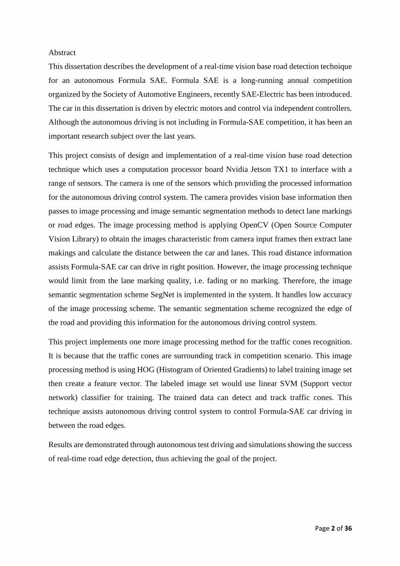
Abstract
This dissertation describes the development of a real-time vision base road detection technique
for an autonomous Formula SAE. Formula SAE is a long-running annual competition
organized by the Society of Automotive Engineers, recently SAE-Electric has been introduced.
The car in this dissertation is driven by electric motors and control via independent controllers.
Although the autonomous driving is not including in Formula-SAE competition, it has been an
important research subject over the last years.
This project consists of design and implementation of a real-time vision base road detection
technique which uses a computation processor board Nvidia Jetson TX1 to interface with a
range of sensors. The camera is one of the sensors which providing the processed information
for the autonomous driving control system. The camera provides vision base information then
passes to image processing and image semantic segmentation methods to detect lane markings
or road edges. The image processing method is applying OpenCV (Open Source Computer
Vision Library) to obtain the images characteristic from camera input frames then extract lane
makings and calculate the distance between the car and lanes. This road distance information
assists Formula-SAE car can drive in right position. However, the image processing technique
would limit from the lane marking quality, i.e. fading or no marking. Therefore, the image
semantic segmentation scheme SegNet is implemented in the system. It handles low accuracy
of the image processing scheme. The semantic segmentation scheme recognized the edge of
the road and providing this information for the autonomous driving control system.
This project implements one more image processing method for the traffic cones recognition.
It is because that the traffic cones are surrounding track in competition scenario. This image
processing method is using HOG (Histogram of Oriented Gradients) to label training image set
then create a feature vector. The labeled image set would use linear SVM (Support vector
network) classifier for training. The trained data can detect and track traffic cones. This
technique assists autonomous driving control system to control Formula-SAE car driving in
between the road edges.
Results are demonstrated through autonomous test driving and simulations showing the success
of real-time road edge detection, thus achieving the goal of the project.

Page 3 of 36
Acknowledgements
I would like to thank the following people for their assistance throughout the course of this
project:
Prof. Thomas Bräunl for his guidance, advice, and supervision throughout the project.
The 2017 Autonomous SAE Team Leader Thomas Drage for his support and project
management.
The 2017 Autonomous SAE Team, vision division Kai Li Lim for his support and
assistance.
The other two members of the 2017 Autonomous SAE Team, Samuel Evans-Thomson
and Mitchell Poole for their assistance and collaboration.
My friends and family for their support and encouragement over the course of the year.

Page 4 of 36
Nomenclature
GPS Global Positioning System
GPU Graphics Processing Unit
HOG Histogram Oriented Gradient
HSL Hue, Saturation, Lightness
HSV Hue, Saturation, Value
IMU Inertial Measurement Unit
LiDAR Light Density and Ranging
LUV CIE 1976 (L*, u*, v*) colour space
REV Renewable Energy Vehicle Project
SAE Society of Automotive Engineers
SVC Support Vector Machine Classifiers
SVM Support Vector Machines
UWA University of Western Australia
YUV YUV colour space
YCrCb YCrCb colour space

Page 5 of 36
Table of Contents Abstract ................................................................................................................................................... 2
Acknowledgements ................................................................................................................................. 3
Nomenclature .......................................................................................................................................... 4
1. Introduction ..................................................................................................................................... 7
1.1 Background ................................................................................................................................... 7
1.2 Motivation ..................................................................................................................................... 7
1.3 Project Delimitations ..................................................................................................................... 8
1.4 Report Layout ............................................................................................................................... 9
2. Literature review ........................................................................................................................... 11
3. System Design .............................................................................................................................. 12
3.1 Overview ..................................................................................................................................... 12
3.2 Software Framework ................................................................................................................... 13
4. Image processing .......................................................................................................................... 14
4.1 Lane Marking Detection ............................................................................................................. 14
4.1.1. Real road distance measurement ......................................................................................... 14
4.1.2. Distortion correction ........................................................................................................... 15
4.1.3. Image thresholding .............................................................................................................. 16
4.1.4. Perspective transformation .................................................................................................. 17
4.1.5. Locate road marking ........................................................................................................... 19
5. Machine learning .......................................................................................................................... 20
5.1 Traffic cone detection ................................................................................................................. 20
5.1.1. Feature Extraction ............................................................................................................... 20
5.1.2. Training ............................................................................................................................... 23
5.1.3. Searching objects ................................................................................................................ 24
5.1.4. Thresholding ....................................................................................................................... 25
5.1.5. Position calculation ............................................................................................................. 26
5.2 SegNet ......................................................................................................................................... 27
5.2.1. Data collection .................................................................................................................... 27
5.2.2. Training SegNet .................................................................................................................. 27
5.2.3. Implement SegNet algorithm on NVIDIA Jetson TX1 ....................................................... 28
6. Integration ..................................................................................................................................... 29
6.1 Software communication ............................................................................................................ 29
6.2 Software Environment Control ................................................................................................... 29
7. Results ........................................................................................................................................... 31
7.1 Lane Marking Detection ............................................................................................................. 31

Page 6 of 36
7.2 Traffic Cones Detection .............................................................................................................. 31
7.3 SegNet ......................................................................................................................................... 32
8. Conclusion and Future work ......................................................................................................... 33
8.1 Conclusion .............................................................................................................................. 33
8.2 Future Work ............................................................................................................................ 33
9. References ..................................................................................................................................... 35

Page 7 of 36
1. Introduction
1.1 Background
The Autonomous SAE car project is based on the REV project's 2010 SAE Electric car which
was developed from an earlier UWA Motorsport car.
The purpose of this project is that providing vision and sensors assist the autonomous SAE car
driving autonomously. This dissertation mainly focusses on vision base detection on road
objects that is going through the computer vision to do image processing. The results would
provide autonomous SAE car to make more accuracy of driving decisions. This project will
cooperate with two other projects. Samuel Evans-Thomson will provide the LiDAR sensor
base road detection to help autonomous drive decision and Mitchell Poole will provide the
IMU and GPS base road detection to help drive the decision of autonomous. The Autonomous
SAE car is a project to provide a platform for autonomous car research. This project build by
previous UWA research that has been done the autonomous mode drive base on recorded GPS
waypoint. However, this result still restrains from GPS accuracy and limited recorded waypoint.
This project intends to improve autonomous mode driving by visual assistance. Therefore, this
project will help the University to researching into fully autonomous vehicles. This
autonomous car also helps to promote the REV project.
1.2 Motivation
This project is proposed to develop the visual base road detection algorism to assist the
autonomous SAE car to do more advance drive decision. The previous developed autonomous
driving algorithm was relying on GPS signal to planning the driving path. However, the GPS
signal strength and accuracy would be restricted to the autonomous diving functionality.
Therefore, to improve the autonomous driving capability is utilizing different sensors and
vision ability, it needs to fusion different incoming data from sensors and vision then do a better
driver decision. The visual image is one of the useful data also very easy to acquire. This project
was developed real-time image detection and recognition functions to improve autonomous
SAE car’s capability.
Page 8 of 36
1.3 Project Delimitations
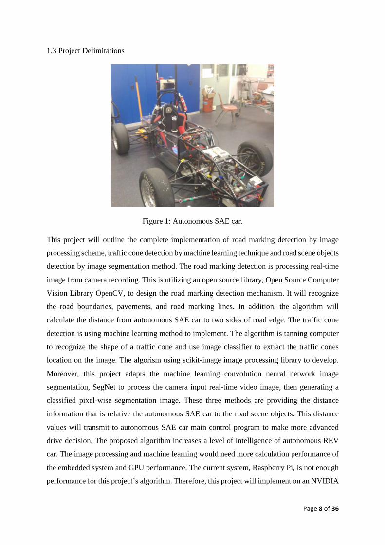
Figure 1: Autonomous SAE car.
This project will outline the complete implementation of road marking detection by image
processing scheme, traffic cone detection by machine learning technique and road scene objects
detection by image segmentation method. The road marking detection is processing real-time
image from camera recording. This is utilizing an open source library, Open Source Computer
Vision Library OpenCV, to design the road marking detection mechanism. It will recognize
the road boundaries, pavements, and road marking lines. In addition, the algorithm will
calculate the distance from autonomous SAE car to two sides of road edge. The traffic cone
detection is using machine learning method to implement. The algorithm is tanning computer
to recognize the shape of a traffic cone and use image classifier to extract the traffic cones
location on the image. The algorism using scikit-image image processing library to develop.
Moreover, this project adapts the machine learning convolution neural network image
segmentation, SegNet to process the camera input real-time video image, then generating a
classified pixel-wise segmentation image. These three methods are providing the distance
information that is relative the autonomous SAE car to the road scene objects. This distance
values will transmit to autonomous SAE car main control program to make more advanced
drive decision. The proposed algorithm increases a level of intelligence of autonomous REV
car. The image processing and machine learning would need more calculation performance of
the embedded system and GPU performance. The current system, Raspberry Pi, is not enough
performance for this project’s algorithm. Therefore, this project will implement on an NVIDIA
Page 9 of 36
Jetson TX1 platform. It can provide more powerful calculation and GPU performance. The
scope of this project will include installation of new Jetson TX1 platform on the autonomous
SAE car, development of proposed algorithm software, a development the communication
tunnel between different software language, and improvement of autonomous SAE electronic
system.
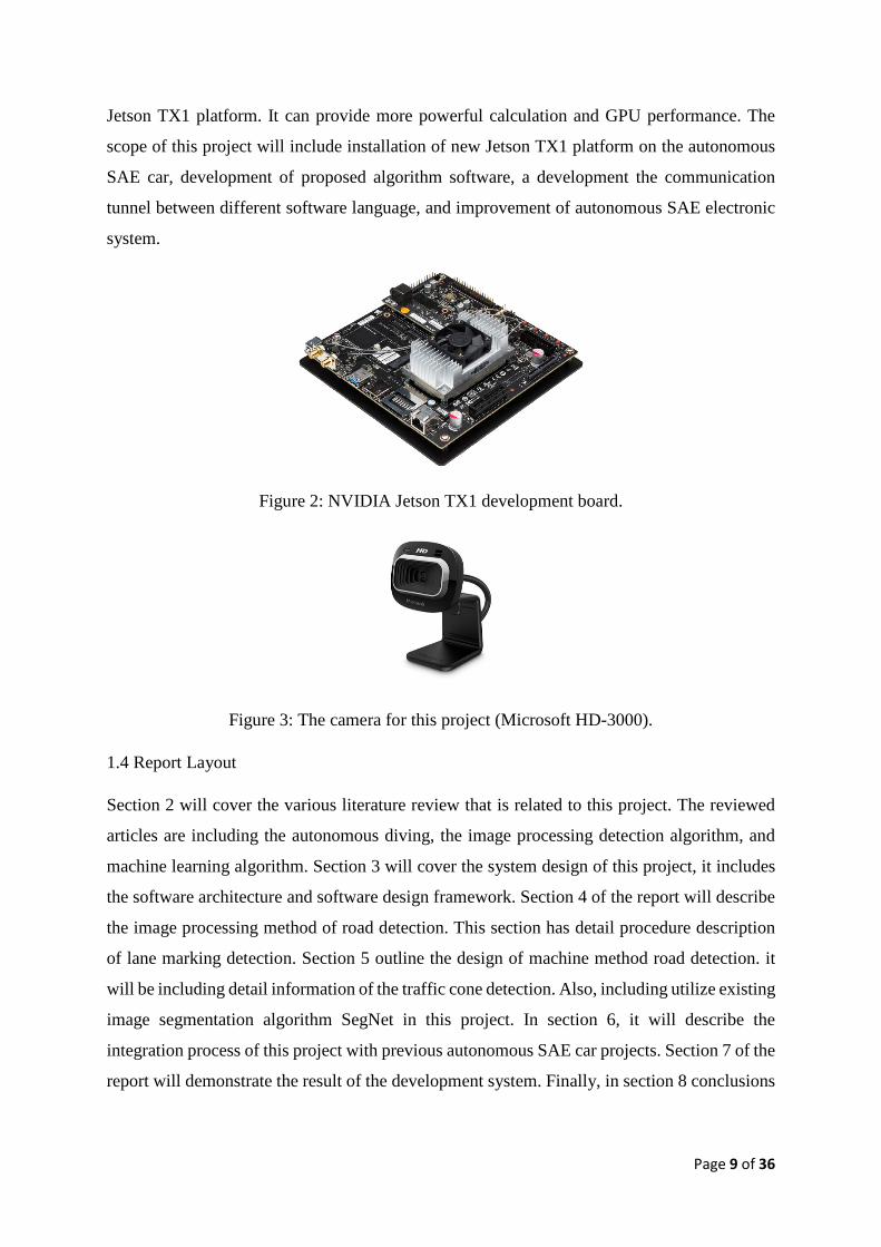
Figure 2: NVIDIA Jetson TX1 development board.
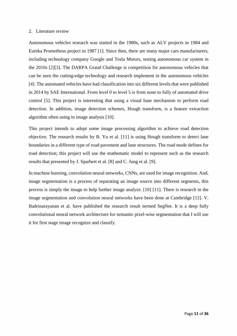
Figure 3: The camera for this project (Microsoft HD-3000).
1.4 Report Layout
Section 2 will cover the various literature review that is related to this project. The reviewed
articles are including the autonomous diving, the image processing detection algorithm, and
machine learning algorithm. Section 3 will cover the system design of this project, it includes
the software architecture and software design framework. Section 4 of the report will describe
the image processing method of road detection. This section has detail procedure description
of lane marking detection. Section 5 outline the design of machine method road detection. it
will be including detail information of the traffic cone detection. Also, including utilize existing
image segmentation algorithm SegNet in this project. In section 6, it will describe the
integration process of this project with previous autonomous SAE car projects. Section 7 of the
report will demonstrate the result of the development system. Finally, in section 8 conclusions

Page 10 of 36
are drawn about the effectiveness of the design for the autonomous SAE car. There are have
recommendations for the future work.
Page 11 of 36
2. Literature review
Autonomous vehicles research was started in the 1980s, such as ALV projects in 1984 and
Eureka Prometheus project in 1987 [1]. Since then, there are many major cars manufacturers,
including technology company Google and Tesla Motors, testing autonomous car system in
the 2010s [2][3]. The DARPA Grand Challenge is competition for autonomous vehicles that
can be seen the cutting-edge technology and research implement in the autonomous vehicles
[4]. The automated vehicles have had classification into six different levels that were published
in 2014 by SAE International. From level 0 to level 5 is from none to fully of automated drive
control [5]. This project is interesting that using a visual base mechanism to perform road
detection. In addition, image detection schemes, Hough transform, is a feature extraction
algorithm often using in image analysis [10].
This project intends to adopt some image processing algorithm to achieve road detection
objective. The research results by B. Yu et al. [11] is using Hough transform to detect lane
boundaries in a different type of road pavement and lane structures. The road mode defines for
road detection; this project will use the mathematic model to represent such as the research
results that presented by J. Sparbert et al. [8] and C. Jung et al. [9].
In machine learning, convolution neural networks, CNNs, are used for image recognition. And,
image segmentation is a process of separating an image source into different segments, this
process is simply the image to help further image analyze. [10] [11]. There is research in the
image segmentation and convolution neural networks have been done at Cambridge [12]. V.
Badrinarayanan et al. have published the research result termed SegNet. It is a deep fully
convolutional neural network architecture for semantic pixel-wise segmentation that I will use
it for first stage image recognize and classify.

Page 12 of 36
3. System Design
3.1 Overview
Figure 4 shows that the software architecture of proposed visual assistance method for
autonomous SAE car. This system will implement on the NVIDIA Jetson TX1 platform. First,
the architecture uses a camera to provide real-time video input which installed at front of
autonomous SAE car. The software is including three parts in this project development. First,
the road marking detection algorism would receive the camera image source to do image
processing. The road marking detection is utilizing conventional image processing to recognize
the road marking then implement the edge detection and distance estimation scheme to
extracting the distance information for driving assistance. Second, the traffic cone detection is
adapting machine learning method to detect traffic cone on the video frames. This algorism
would be detected the traffic in front of the car then estimate the relative distance for the driving
decision program. The existing image segmentation algorithm SegNet which is fully
convolutional neural network architecture for semantic pixel-wise segmentation. The results of
SegNet are classified images which use a different colour to represent a different type of objects.
The classified images would be helped the road boundary detection during the road marking
and traffic cone detection failed. Finally, these three algorisms providing the road detection
result to the distance estimation procedure then feedback the road detection information for the
current autonomous SAE car to make drive decision.
Figure 4: The software architecture of proposed method.

Page 13 of 36
3.2 Software Framework
The autonomous vehicles need visual scene understanding algorisms to recognize and identify
the objects at front of vehicle. The image processing algorithm is important for this project.
Recently, more and more machine learning image segmentation research has been done. These
research results are helpful to develop this project.
The main objective of this project is using the real-time image for road detection. Therefore,
image detection algorithm development is the core of this project. The literature review is an
important stage for design algorithm.
This algorism can operate in real-time and run on low-power devices. Therefore, this project
is trying to implement the proposed algorism and image segmentation algorithm, SegNet, on
the multicore GPU solution, NVIDIA Jetson TX1.
Autonomous formula SAE vehicle would use visual information to be one of reference for the
driving decision. Image data obtained from the camera is processed was the most important
thing for this project. This part mainly uses a camera to collect images then to apply OpenCV
(Open Source Computer Vision Library) and SegNet (a deep learning framework pixel-wise
image semantic segmentation) for road edges detection. OpenCV provides many modules, such
as image processing, video, and video I/O, that is useful for road edges detection. However,
using OpenCV for image recognition is limited by image quality, brightness, and contrast.
SegNet is an image semantic segmentation approach. It can classify road scene objects, such
as the pedestrian, lane marking, traffic light, vehicles etc., that complement the insufficient of
single image processing methods.

Page 14 of 36
4. Image processing
The programming language is Python for the image processing. Since it can compatible with
many open source image processing libraries such as OpenCV, scikit-image libraries.
4.1 Lane Marking Detection
4.1.1. Real road distance measurement
The main road detection algorithm is a post-processing scheme after the image received
from the camera. Firstly, the real distance measurement from the image is needed for the
road detection algorism. Figure 5 shows that a road model of distance measurement. The
bollards are the anchor point that will help positioning and calculation the point and
distance. This image is from the camera which installs on autonomous SAE car, the
resolution of the image is 800x600.
Figure 5: The model of road distance measurement.
Figure 6 shows that the values of the real road model. The values of road model can be
mapping to the camera captured image. The image resolution of the processed image is
smaller than the original image resolution. Therefore, the real distance from the image
processing output must be proportional to the original one.

Page 15 of 36
Figure 6: The values of the distance of road model.
4.1.2. Distortion correction
This project is using a conventional webcam as video input camera which is the cheap
pinhole camera. Unfortunately, this camera has distortion that caused by the optical design
of lenses, that result in some kind of deformation of images. Therefore, the images need to
do calibration before image processing. OpenCV provides camera calibration function to
correct this distortion. Furthermore, with calibration, the distance of the road can be
determined more accurately. It is because the results of this OpenCV function improving
the accuracy of the relation between the camera’s natural units (pixels) and the real-world
units (meters). The first step for the image processing is camera calibration to get a
undistorted image. This is using chessboard image and finding chessboard corners to get
two accumulated lists, 3D point in real-world space and 2D points in an image plane. Then
use the camera calibrate function in OpenCV library to obtain the camera calibration and
distortion coefficients [13]. This scheme would remove the camera distortions. The results
are shown in figure 7 that the distortion image can be correct effectively.

Page 16 of 36
Figure 7: Chessboard distortion correction.
4.1.3. Image thresholding
A camera input image is a number of combinations of colour that image was very unstable
since changing conditions in lighting and contrast. Therefore, the image has to convert into
the grayscale image to decrease the instability. After that use filter smoothing the image to
reduce the image noise. This processed image pass to the other OpenCV function to get the
edge information. Using canny edge detection extract structure information from the
grayscale image. Canny edge detection has high noise tolerance and low error rate. After
that, the algorithm can easier to get the road boundary information [14]. Road edges
detection scheme detects lane-marking at two sides of autonomous SAE vehicle. The road
marking detection utilize OpenCV library. Finding the edges of the whole image is
reducing the image complexity because numbers of colour and gradient of the image would
make the image processing more difficult. A canny edge detection is a convenient approach
in OpenCV library [15]. The results are shown in figure 8 that the image converted into
edge only binary image.
Figure 8: Threshold image processing.

Page 17 of 36
4.1.4. Perspective transformation
The edge image has produced from the previous step, then investigate the edge image and
finding the vanishing point, it will help to find the anchor point on the processed image.
Figure 9 demonstrates that an example processed image. At the middle of the image is a
vanishing point. This point is the end of the road in this image view. Therefore, it can be
found the around upper 40 percent of the image is redundant. Hence, it can mask out this
region to decrease the process loading.
Figure 9: Example processed image and road model.
Now, the road marking has shown on the edge image clearly, since the road markings are
approximated as lines, it can be used to extract four points that are actually on the road.
then use Hough transforms to detect the left and right road markers that are at two sides of
autonomous SAE vehicle. Hough transform is using for recognizing the road boundaries.
The road boundaries or edges are a pair of a straight line. Hence, it can use a parametric or
normal equation to represent.
𝑥𝑥𝑥𝑥𝑥𝑥𝑥𝑥𝑥𝑥 + 𝑦𝑦𝑥𝑥𝑦𝑦𝑦𝑦𝑥𝑥 = 𝑟𝑟

Page 18 of 36
Where r is the length from original to this line and 𝑥𝑥 is the orientation of r with respect to
x-axis.
Figure 10: Parametric description of a straight line [16].
The road modeling will be done after the Hough transform. The parameters are shown in
figure 9. Where ymax is located at the vanishing point, it means the end of the road. ymin is
the closest distance to the car. The algorithm will pick a y value between ymax and ymin for
the best position to feedback road distance. Where the Pmiddle is the middle position where
the car is. Then Pleft and Pright is the point corresponding to Hough transform line detection.
The making of lanes is detected then using perspective transforms to get a bird’s view of
the image. It can easily find 4 points to represent two-lane markings. Finally, using second
order polynomial method fits the points. The perspective transform image shown in figure
11, it converts the image into a bird’s view image.
Figure 11: The perspective transform image.
Page 19 of 36
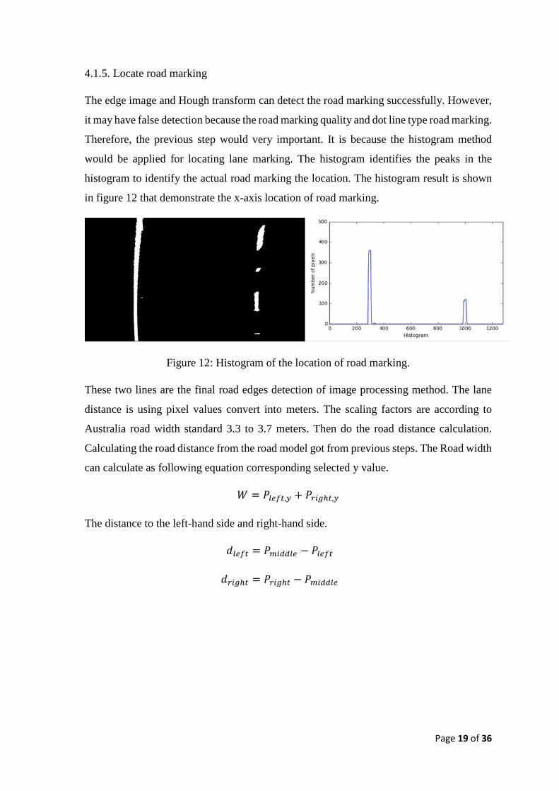
4.1.5. Locate road marking
The edge image and Hough transform can detect the road marking successfully. However,
it may have false detection because the road marking quality and dot line type road marking.
Therefore, the previous step would very important. It is because the histogram method
would be applied for locating lane marking. The histogram identifies the peaks in the
histogram to identify the actual road marking the location. The histogram result is shown
in figure 12 that demonstrate the x-axis location of road marking.
Figure 12: Histogram of the location of road marking.
These two lines are the final road edges detection of image processing method. The lane
distance is using pixel values convert into meters. The scaling factors are according to
Australia road width standard 3.3 to 3.7 meters. Then do the road distance calculation.
Calculating the road distance from the road model got from previous steps. The Road width
can calculate as following equation corresponding selected y value.
𝑊𝑊 = 𝑃𝑃𝑙𝑙𝑙𝑙𝑙𝑙𝑙𝑙,𝑦𝑦 + 𝑃𝑃𝑟𝑟𝑟𝑟𝑟𝑟ℎ𝑙𝑙,𝑦𝑦
The distance to the left-hand side and right-hand side.
𝑑𝑑𝑙𝑙𝑙𝑙𝑙𝑙𝑙𝑙 = 𝑃𝑃𝑚𝑚𝑟𝑟𝑚𝑚𝑚𝑚𝑙𝑙𝑙𝑙 − 𝑃𝑃𝑙𝑙𝑙𝑙𝑙𝑙𝑙𝑙
𝑑𝑑𝑟𝑟𝑟𝑟𝑟𝑟ℎ𝑙𝑙 = 𝑃𝑃𝑟𝑟𝑟𝑟𝑟𝑟ℎ𝑙𝑙 − 𝑃𝑃𝑚𝑚𝑟𝑟𝑚𝑚𝑚𝑚𝑙𝑙𝑙𝑙

Page 20 of 36
5. Machine learning
Machine learning method is popular for the image objects detection recently. Machine learning
is the computer program that is an algorithm that can recognize something would like to detect
in the image. There is two type of machine learning, supervised learning and unsupervised
learning. This project is using supervised learning type of machine learning. Therefore, the
algorithm needs a trained data set for recognizing the object in the image. This project develops
an algorithm to detect traffic cone and adapts existing advanced deep learning algorithms for
road scene objects detection.
5.1 Traffic cone detection
5.1.1. Feature Extraction
Using machine learning to detect traffic cone detection needs to be prepared at least 300
cone images for the algorithm learning the feature of traffic cones. This project was
collected traffic cone images dataset and non-traffic cone images for algorithm comparison.
The image is shown in figure 13 that including traffic cone images and non- traffic cone
images.
The next step is extracting the image feature. It is a necessary step for the supervised
machine learning. Therefore, the image feature is extracting by the Histogram Oriented
Gradient (HOG) feature descriptor. HOG feature descriptor is popular for object detection
[17]. This algorithm provides from the open source image library scikit-image. This
algorithm would do the following computation for the feeding images dataset, computing
the gradient image in x and y, computing gradient histograms, normalizing across blocks,
and flattening into a feature vector.
The first step of this algorithm is applying a global image normalization which is used for
illumination effects reduction. Usually, it applies gamma compression that commuting the
square root of each colour channel. The result is image texture strength that is proportional
to the surface illumination. Therefore, this compression is able to reduce the image
shadowing and illumination. Next step is computing first order image gradients. This step
would get the image contour or edge information. Then put it into previous illumination
variations results. On the other hand, the local colour channel provides colour invariance.
Combined these results that would be an original detector. The third step is to do encoding
sensitive local image. Then the image divides into a number of small spatial regions (cells).
In each cell do the one dimension histogram of edge orientation for each pixel in local cell.

Page 21 of 36
Figure 13: Traffic cone images and non-traffic cone images.
This one dimension histogram basically is orientation histogram. Every cell has this
orientation histogram, then divide gradient angle into previous image calculation results.
The gradient magnitude is used to vote the orientation histogram. The fourth step is
computing normalization which grouping the local cells and calculating normalize. The
normalized procedure would improve the invariance to different factors such as
illumination and shadowing. The local group of cells that called blocks. The normalized
result is applying in every cell of the block. Therefore, the normalize would do much time
for final output vector. It used many calculating sources but improved the performance.
This normalized block descriptor is basically being Histogram of Oriented Gradient (HOG)

Page 22 of 36
feature descriptor [17]. The final step is collecting all of the results in the previous step. All
blocks normalized results convert into a combined feature vector. The cone HOG future
descriptor result shown in figure 14.
Figure 14: HOG feature descriptor results.
The colour channel and different parameter setup are influenced the performance of
extracting time of the HOG feature descriptor. This project has experimented different
combination of parameters. The results show that the YUV colour space, 16 pixels per cell,
2 cells per block, and ALL HOG channel have better performance.
Test setting Colour
space Orientations
Pixels per
cell
Cells per
block
HOG
channel Time
1 HSL 9 8 2 1 26.40s
2 HSL 9 8 2 ALL 73.97 s
3 HSV 9 8 2 1 35.47 s
4 HSV 9 8 2 ALL 54.74 s
5 LUV 9 8 2 1 35.35 s
6 LUV 9 8 2 ALL 60.09 s
7 YCrCb 9 8 2 1 38.25 s
8 YCrCb 9 8 2 ALL 58.65 s
9 YUV 9 8 2 ALL 48.90 s
10 YUV 11 16 2 ALL 42.83 s
Table 1: HOG feature descriptor extracting time experiment results.

Page 23 of 36
5.1.2. Training
While the image future descriptor algorithm is ready, then the algorism can do the training.
The dataset training needs to extract input datasets and combine. The previous section has
defined 10 different combinations of HOG feature description parameters. Then test the
extracting speed for all datasets. The results are extracted from the HOG feature descriptor
would shuffle and split into training and test. This step feeds all feature vector of datasets
into a linear support vector machine (SVM) classifier. The propagation after linear SVC
would be the training time, and the shuffled datasets would test the accuracy. Table 2 shown
that 10th parameter setup got the best accuracy and reasonable training time. Therefore, this
project would use this setup as the default setting.
Test setting Classifier Accuracy Train time
1 Linear SVC 99.56 1.81 s
2 Linear SVC 99.56 3.03 s
3 Linear SVC 99.62 1.64 s
4 Linear SVC 99.84 27.96 s
5 Linear SVC 99.73 0.61 s
6 Linear SVC 99.84 11.42 s
7 Linear SVC 99.78 4.85 s
8 Linear SVC 99.83 10.62 s
9 Linear SVC 99.84 8.31 s
10 Linear SVC 99.95 3.72 s
Table 2: HOG feature descriptor with linear SVC training time and accuracy.
The classifier is applying linear SVC classifier which is including scikit-learn machine
learning library for the Python programming language. This classifier is based on support
vector machines (SVMs) to development. The SVMs is a supervised machine learning
methods. It is wildly applying at classification, regression, and outliers’ detection. there are
the SVMs advantages such as effective in high dimensional spaces, allow the number of
dimensions greater than the number of samples, it uses a subset for tanning (support vectors)
in the decision function, Memory efficient, and it support specifies custom kernel for
decision function. However, SVMs also have disadvantages such as do not directly provide
probability estimates and the kernel function and regularization term is hard to define while
the number of features more than the number of samples.

Page 24 of 36
5.1.3. Searching objects
This section describes the method for detecting traffic cones in an image. It needs the
trained data which was prepared by the previous steps. This method using HOG feature
extraction again, then applying sliding windows to searching the specific objects in an
image. However, extracting features and searching the object in the entire image is time-
consuming. Therefore, this algorithm has selected a portion of the image the perform the
HOG features extraction first. Then use this extracted feature image doing subsample by
different size of windows across a selected range of the image. This selected range of image
feeding into the linear SCV classifier. The algorithm performs the classifier prediction base
on HOG features for each selected window region. Then the classifier returns the result is
matching traffic cone’s features or not. The figure 15 shows that the window searching
across the image.
Figure 15: Different size of searching windows.
The algorithm has tried different configuration of window size and window overlap. The
previous experiment has tried the smallest size of the window was 0.5 scale of size and 50
and 75 percent of window overlap in both x and y-axis, but the results had too many false
detections. Therefore, the algorithm was increasing the window size to 1x, 1.5x, 2x, and 3x
times of scales and the overlap percentage set as 50 percent. After the four sizes of window
searching finished. Each size of the widow would mark the detected traffic cones’ position.

Page 25 of 36
It is shown in figure 16 that still has false detection in the image. Therefore, it needs a
further algorithm to filter the false detection.
Figure 16: Object searching results with false detection.
5.1.4. Thresholding
The false detection would happen that influence the object detection results. Therefore, the
algorithm has to deal with this problem. Analysing the results from the previous section,
the correct detection would be detected by different size of window searching. Figure 17
shows that the repetition of traffic cone detected by the different window size.
Figure 17: Repetition of traffic cone detected.
The false detections normally show one time only. The algorithm designs a simple filter to
cancel out the false detection. The method is creating a blank image then adding the pixel
value which is a relative position the different window detected the traffic cones. While the
cone position was detected by different size of window searching. The relative position
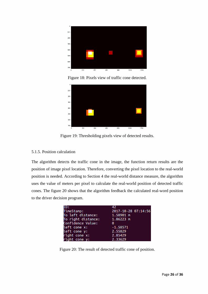
pixel values would greater. Figure 18 shows the repetition of traffic cone detected in pixels
view. The final step is given a threshold for the pixels view to filter out the false detection.
Figure 19 shows that the false detection pixels have been removed.
Page 26 of 36
Figure 18: Pixels view of traffic cone detected.
Figure 19: Thresholding pixels view of detected results.
5.1.5. Position calculation
The algorithm detects the traffic cone in the image, the function return results are the
position of image pixel location. Therefore, converting the pixel location to the real-world
position is needed. According to Section 4 the real-world distance measure, the algorithm
uses the value of meters per pixel to calculate the real-world position of detected traffic
cones. The figure 20 shows that the algorithm feedback the calculated real-word position
to the driver decision program.
Figure 20: The result of detected traffic cone of position.

Page 27 of 36
5.2 SegNet
SegNet is a pixel-wise semantic segmentation in deep learning framework. Semantic
segmentation is to apply for understanding the visual scene and object. This has been widely
adopted in autonomous driving. The architecture of SegNet is a convolution encoder and
decoder which is a pixel-wise classifier. The objects classify from SegNet is including
following classes, sky, Building, column-pole, road-marking, road, pavement, tree, sign-
symbol, fence, vehicle, pedestrian, and bicyclist. The accuracy of classify result is 65.9% for
classes average [12].
The image processing approach road marking detection has a chance to be failed because the
lane markings are not clear or no lane markings. Therefore, adapting existing algorithm SegNet
into this project’s software architecture to supplement image processing method’s insufficient.
The original software has hardware requirement, hence NVIDIA Jetson TX1 cannot run the
program directly. It needs modification of code to reduce hardware requirement. One of the
solutions is decreasing the image resolution. The origin SegNet image resolution is 640 by 480
that caused the memory shortage of Jetson TX1. Adjusting resolution to 320 by 240 can run on
the platform, but the FPS is low to run road detection. Therefore, the resolution 240 by 160 is
the acceptable speed of processing and quality image output.
The input images use the SegNet to do visual scene classification. It would produce the results,
road, road-marking, and pavement, are useful for road edges detection. This algorithm is
similar to machine learning method process to get the classification result. There are the process
steps of SegNet.
5.2.1. Data collection
The SegNet image segmentation mechanism needs a bunch of videos to train the program.
Current SegNet is using CamVid dataset as a training source. It is compatible with the
Australia traffic system. However, to improve the image recognize accuracy use local
traffic video source to train the segmentation program is needed.
5.2.2. Training SegNet
The current SegNet is using CamVid dataset. Therefore, the program can train by local
traffic system, after the video data collected. The training process needs a high GPU
performance computer. It is difficult to do that with low power devices. Hence, the training

Page 28 of 36
process was using dual NVIDIA TITAN X GPU computer that provides by robotics and
automation lab.
5.2.3. Implement SegNet algorithm on NVIDIA Jetson TX1
The image segmentation algorithm SegNet is a research result from V. Badrinarayanan et
al. [12]. The authors provide open source code on GitHub. The results of SegNet shown in
figure 21. The top image is input video source and the button one is the output of
segmentation, the right-hand side shows the colour map of the objects.
Figure 21: The SegNet result on high-performance computer (640x480) [12].

Page 29 of 36
6. Integration
6.1 Software communication
The software development of this project is using Python as the main programming language
because of it compatible with many image processing library and machine learning library.
However, the original autonomous SAE car was using C++ as the main programming language.
The communication between this project’s program and previous main drive decision program
needs an intermediate protocol. Therefore, this project applying the Google Protocol Buffers,
Protobuf, which is a language-neutral, platform-neutral extensible mechanism for serializing
structured data. Protobuf provides protocol between Python and C++. The data format was
defined that including data ID, timestamp, left lane distance, right lane distance, confidence
value, and detected cone position. The data format is shown in the following code block.
Protobuf can generate python and c++ code automatically. Then the algorithm establishes a
UDP connection between it then the data structure can directly provide for main driving
decision program.
package roadDistance; message Lane { required int32 id = 1; required string time = 2; required float left = 3; required float right = 4; required float left_x = 5; required float left_y = 6; required float right_x = 7; required float right_y = 8; required int32 cv = 9; } message roadDistance { repeated Lane lane = 1; }
6.2 Software Environment Control
This project was developing under Ubuntu 16.04 LTS operation system. Therefore, the
operating system environment has to be configurated for software running. The table 3 shows
that the library used for this project.

Page 30 of 36
Python 2.7.12 Numpy
Caffe Matplotlib
CUDA Toolkit Scipy
cuDNN v5 OpenCV
Glob Protobuf
Pickle Scikit-image
Scikit-learn Pillow
Table 3: Software and library usage.

Page 31 of 36
7. Results
7.1 Lane Marking Detection
The result of lane marking detection shown in figure 22 that demonstrate three different
windows which include original video input, bird’s view, and output of road marking detection.
At the output screen, it shows the annotated different colour on the detected road marking.
Moreover, the output screen also shows left and right lane distance simultaneously.
Figure 22: The result of lane marking detection.
7.2 Traffic Cones Detection
The result of traffic cone detection shown in figure 23 that use a blue rectangle to indicate the
traffic cone position. The results also demonstrate the algorithm can recognize the different
colour of traffic cones.

Page 32 of 36
Figure 23: The result of traffic cone detection.
7.3 SegNet
The SegNet output is restrained to Jetson TX1 performance. The output image is noisy, it is
shown in figure 24. The results still can recognize the road, and car objects, hence SegNet is
useful to be a backup algorithm during the road marking detection failed.
Figure 24: The SegNet result on NVIDIA Jetson TX1 (240x160)

Page 33 of 36
8. Conclusion and Future work
8.1 Conclusion
At the beginning of the project, the drive decision control of the autonomous SAE car was
identified to be a failure factor with regards to the accuracy of GPS location accuracy. This
generated a goal to investigate that require the software improve and sensors assistance the
control functionality. Whilst there exists research in the field of vision assistance for
autonomous vehicles, but no result was found the implementation of real-time image
processing method in the autonomous SAE vehicles. This is due to image processing would
require high-performance calculation.
The GPU performance was improved and the size of the embedded system was significantly
reduced. Thus, this project has developed the image processing method and machine learning
method to perform road detection. The algorithm can run on the high-performance GPU
platform NVIDIA Jetson TX1 with autonomous drive speed requirement.
The road marking detection and traffic cone detection was therefore integrated into the vehicle
as a result. The algorithm provides the lane marking distance information and traffic cone
position information to the dive decision program to improve the path planning accuracy of
autonomous SAE car. The test result was overcoming the GPS signal inaccuracy.
Overall, the autonomous SAE car is now able to navigate while driving on paths with better
accuracy, this allows for further research in new areas such as autonomous driving in
competitive environments.
8.2 Future Work
In terms of potential research to the road detection ability of the vehicle, the extension of the
algorithm capable use multiple cameras for the image processing. There is some research using
two cameras to measure the real-world distance. It can improve the method used in this project.
The GPU programming is one of a method to improve the program running speed. The
algorithm in this project has been applied it to improve the speed. However, some of the third-
party libraries did not support the GPU programming. For the future implementation, using
entire GPU programming for the algorithm would need for more complex algorithm
development.

Page 34 of 36
The machine learning can be having more improvement. The deep learning research results
have more and more been published. This is will help autonomous SAE car processing the
image input with reliable, accurate, and fast for the diving control.
Page 35 of 36
9. References
[1] "Autonomous car", wikipedia.org, 2017. [Online]. Available:
http://en.wikipedia.org/wiki/Autonomous_car.
[2] "History of autonomous cars", wikipedia.org, 2017. [Online]. Available:
https://en.wikipedia.org/wiki/History_of_autonomous_car.
[3] "Tesla Autopilot", wikipedia.org, 2017. [Online]. Available:
https://en.wikipedia.org/wiki/Tesla_Autopilot.
[4] "DARPA Grand Challenge", wikipedia.org, 2017. [Online]. Available:
https://en.wikipedia.org/wiki/DARPA_Grand_Challenge.
[5] System Classification and Glossary. Automated Driving Applications and
Technologies for Intelligent Vehicles, 2017.
[6] "Hough transform", wikipedia.org, 2017. [Online]. Available:
https://en.wikipedia.org/wiki/Hough_transform.
[7] B. Yu and A. Jain, "Lane boundary detection using a multiresolution Hough
transform", Proceedings of International Conference on Image Processing.
[8] J. Sparbert, K. Dietmayer and D. Streller, "Lane detection and street type
classification using laser range images", ITSC 2001. 2001 IEEE Intelligent Transportation
Systems. Proceedings (Cat. No.01TH8585).
[9] C. Jung and C. Kelber, "A robust linear-parabolic model for lane following",
Proceedings. 17th Brazilian Symposium on Computer Graphics and Image Processing.
[10] "Convolutional neural network", wikipedia.org, 2017. [Online]. Available:
https://en.wikipedia.org/wiki/Convolutional_neural_network.
[11] "Image segmentation", wikipedia.org, 2017. [Online]. Available:
https://en.wikipedia.org/wiki/Image_segmentation.
[12] V. Badrinarayanan, A. Kendall and R. Cipolla, "SegNet: A Deep Convolutional
Encoder-Decoder Architecture for Scene Segmentation", IEEE Transactions on Pattern
Analysis and Machine Intelligence, pp. 1-1, 2017.

Page 36 of 36
[13] "Camera Calibration — OpenCV-Python Tutorials 1 documentation", Opencv-
python-tutroals.readthedocs.io, 2017. [Online]. Available: https://opencv-python-
tutroals.readthedocs.io/en/latest/py_tutorials/py_calib3d/py_calibration/py_calibration.html#c
alibration.
[14] "Canny edge detector", wikipedia.org, 2017. [Online]. Available:
https://en.wikipedia.org/wiki/Canny_edge_detector.
[15] "Canny Edge Detection — OpenCV-Python Tutorials 1 documentation", Opencv-
python-tutroals.readthedocs.io, 2017. [Online]. Available: https://opencv-python-
tutroals.readthedocs.io/en/latest/py_tutorials/py_imgproc/py_canny/py_canny.html.
[16] "Image Transforms - Hough Transform", Image Processing Learning Resources,
2017. [Online]. Available: http://homepages.inf.ed.ac.uk/rbf/HIPR2/hough.htm.
[17] Dalal, N. and Triggs, B., “Histograms of Oriented Gradients for Human Detection,”
IEEE Computer Society Conference on Computer Vision and Pattern Recognition, 2005, San
Diego, CA, USA.