Aggregate Reallocation Shocks, Occupational Employment and

Distance

Jacob Wong The University of Adelaide

Working Paper No. 2017-09 May 2017

Copyright the author

School of Economics

Working Papers ISSN 2203-6024

Aggregate Reallocation Shocks, OccupationalEmployment and Distance

JACOB WONG∗

The University of Adelaide

This version : May 24, 2017

Abstract

A unique general equilibrium model featuring many occupations and aggregateshocks is created to study occupational employment dynamics by imposing a corre-lated TFP structure across occupations along with distance between occupations.Productivity processes across occupations are correlated with similar occupationsexperiencing similar fluctuations. Mobility frictions and the correlated-productivitystructure produce a systematic relationship between occupational employment cor-relations and occupational distance that does not arise when productivity processesare independent. Using employment data and measures of task-distance betweenoccupations from the U.S. economy, a negative relationship between the correla-tion of occupational employment and task-distance separating occupation-pairs isuncovered.

KEYWORDS: Labour reallocation, Occupation switching, Task-distanceJEL CLASSIFICATION: E24, J24, J31, J62

∗School of Economics, The University of Adelaide, Adelaide, SA 5005, Australia. Email: ja-cob.wong@adelaide.edu.au. Thanks to Chris Edmond, Aspen Gorry, William Hawkins, Nicolas Jacquet,Nicolas Petrosky-Nadeau, Petr Sedlacek, Serene Tan, Lawrence Uren, Venky Venkateswaren, and MarkWeder for valuable comments. Especial thanks to Paul Beaudry, Fabrice Collard, Francisco Gonzalezand Stephanie McWhinnie. This research is supported by a grant from the Australian Research Council(DP140102869).

1. INTRODUCTION

There is a dearth of models currently available to study the general equilibrium ef-

fects of aggregate shocks on costly labour reallocation that feature many heterogeneous

labour markets. Hence, implications concerning dynamics that may arise from standard

assumptions embedded in static general equilibrium models remain uninvestigated. An

intuitive view regarding the effects of supply or demand shocks on labour markets is that

similar labour markets should exhibit similar responses to these shocks. For example,

technological innovations that complement a particular set of tasks likely confer similar

productivity benefits to all occupations that employ these tasks in comparable manners.

Furthermore, these occupations likely experience similar employment responses condi-

tional on such shocks. Formalizing such intuition to derive testable implications requires

a theory that incorporates a notion of distance between labour markets (to measure

similarity) and structure on the random disturbances that alter the relative returns to

employment across labour markets. Without assuming away the distributional effects of

relative supply and demand, a difficulty arises as multiple distributions must be tracked

in order to solve for an equilibrium. By confronting this difficulty, a framework is created

in this paper to study costly labour reallocation in response to aggregate shocks that

have differential impacts across occupations depending on their similarity of the tasks

required for production. A stark qualitative property arises from the model relating the

correlation of employment across occupations to their relative distance. Data from the

U.S. economy shows that such a qualitative relationship exists.

A unique model of occupational choice is presented that features aggregate shocks

and a notion of distance between occupations. The aggregate reallocation shocks in-

troduced in this paper are shocks that simultaneously change the occupation-level total

factor productivity (TFP) across all occupations in the economy. A correlation structure

across occupational TFP is imposed with the correlation of TFP between any two occu-

pations being a function of the distance that separate them. The distance that separates

any occupation-pair represents the dissimilarity between the tasks required by the two

occupations. Distance also dictates the costs required of an individual who wishes to

switch between the two occupations. By tying the correlation of productivity between

occupations to their relative distances, this paper offers a granular view concerning the

differential effects that aggregate shocks can have across occupations.

Within the model, workers are distributed across a continuum of occupations. Each

1

occupation produces an intermediate good that is used in the production of a final con-

sumption good. At any point in time a given worker possesses skills to work in a particular

occupation. Every occupation has its own level of labour productivity and all occupa-

tions experience fluctuations in labour productivity over time. Each period, all workers

face an idiosyncratic fixed cost of retraining. Furthermore, if a worker chooses to retrain,

the cost of switching to an occupation that uses different tasks relative to the worker’s

current occupation is high in comparison to switching to an occupation using similar

tasks relative to the worker’s current occupation. Workers face the option of working, or

not working for the period, and retraining in order to have the skills to work in a different

occupation next period.

Over time, the economy is buffeted by reallocation shocks which can be interpreted

as technological innovations that favour some occupations at the expense of others. The

effect of the fixed costs of retraining as well as convex costs of retraining to dissimilar

occupations is that the distribution of workers across occupations changes over time.

This in turn affects the wage distribution across occupations. The distribution of wages

feeds back into the equilibrium decisions of workers to retrain generating an interplay

between the distribution of employment across occupations and the wage distribution.

Solving for the equilibrium of this economy requires the ability to keep track of the dis-

tributions of workers across occupations as well as the distribution of labour productivity

across occupations. As the distributions of workers across occupations has no analytical

solution and can play an economically significant role, numerical methods are used to

study the equilibrium dynamics. Two assumptions are used to manage the computa-

tional difficulties of tracking these two infinite dimensional objects. The first assumption

is that occupations are located on the circumference of a circle; in other words, there

is an occupation ring. The greater the distance between two occupations on the ring,

the more dissimilar the tasks used by the occupations in production. The second mod-

elling assumption is that the relative productivity across occupations in relation to the

most productive occupation is preserved across time. However, the identity of the most

productive occupation can change over time. In this specific sense, a reallocation shock

can be modelled simply as a change in the identity of the most productive occupation.

Once the identity of the most productive occupation is known the relative productivity

of all other occupations can be determined. These modelling assumptions reduce the

computational problem to that of tracking the distribution of workers across occupations

and tracking the identity of the most productive occupation.

2

The geometrical representation of occupations around a ring, along with the corre-

lation across productivities by distance, results in a way of viewing an intuitive type

of aggregate shock that differs from the typical aggregate TFP shock that is employed

in macroeconomic models. In order to determine whether such a productivity struc-

ture is plausible, U.S. wage data from the CPS Merged Outgoing Rotation Groups and

employment data from the CPS Basic Monthly Files are used along with the model’s

assumptions on the production functions and perfect competition to obtain a measure of

average relative labour productivity between a large number of occupation-pairs. With

these measures of average labour productivity in hand along with standard measures

of task-distance between occupation-pairs, a relationship between task-distance separat-

ing occupation-pairs and relative average labour productivity is estimated. Revealed

by this process is an increasing relationship between relative labour productivity across

occupation-pairs and the task-distance that separates them. This observation bestows

some credibility upon the model.

A stark implication of the model is that the correlation of employment per-capita

(or employment shares) between occupation-pairs should be related to a measure of dis-

tance that separates the occupations. In contrast, when shocks to occupational TFP

are independent across occupations, no systematic relationship arises in the correlation

of employment between occupation-pairs and the distance that separates them. Revisit-

ing the occupational employment data and the task-distance data, a simple econometric

model is employed to highlight a negative relationship between the correlation of em-

ployment across occupation-pairs and the task-distance that separates them; on average,

as the distance between occupation-pairs increase, the less positive is their correlation of

employment. It is shown that while this relationship holds across a large set of occupa-

tions, it also obtains when examining only occupations that are traditionally classified

as requiring routine manual tasks and when only examining occupations that are tradi-

tionally classified as requiring the performance of non-routine cognitive tasks. This lends

some additional value to modelling occupations at a granular level.

From the modelling perspective, the literature most related to the model in this paper

is that which has grown from the seminal paper of rational expectations, general equilib-

rium unemployment by Lucas and Prescott (1974). In their paper, Lucas and Prescott

introduced a theory of equilibrium unemployment in which workers are attached to is-

lands that, in this paper’s context, may be thought of as occupations. Occupations are

subject to idiosyncratic demand shocks that generate wage differentials across occupa-

3

tions. Each worker chooses either to work at their occupations’s prevailing wage, switch

to a different occupation or stay attached to their current occupation and wait for better

times. The model in the present paper adds a measure of distance between occupations

with distance representing a notion of task-similarity between occupations. The cost

that a worker incurs when switching occupations increases as the dissimilarity of tasks

increases relative to the worker’s current occupation. The assumption that task-distance

is relevant for labour market decisions at the individual level seems reasonable if task-

capital is lost when switching between occupations requiring dissimilar task usage. This

reasoning has been argued to be consistent with observations on occupation switching

in work by Poletaev and Robinson (2008), Gathmann and Schonberg (2010), Robinson

(2010) and Cortes and Gallipoli (2017). In the classic Lucas-Prescott island model occu-

pation switching is not directed; when workers decide to switch islands, they sit out of

the labour force for a period and then have unrestricted choice of islands upon which to

reenter the labour force.

Aside from intuitive appeal, incorporating distance enables the formulation of aggre-

gate reallocation shocks allowing for the examination of out-of-steady-state dynamics.

Most applications of the Lucas-Prescott island model that incorporate many islands

along with general equilibrium effects have examined steady state implications.1 There

exists a body of research using the Lucas-Prescott island model to examine the effects

of aggregate shocks on unemployment. These applications, typically assume that there

are only two islands thereby minimizing the distributional complexity involved in solving

for equilibrium outcomes. For example, Gouge and King (1997) as well as Garin et al.

(2017) use a two-island model to examine the relationships between productivity and

unemployment. The model constructed in this paper complements this previous work by

incorporating distance between islands with a large number of islands so that a richer

set of questions may be addressed by the model.2 Pilossoph (2014) uses a two-island

Lucas-Prescott island model to examine the effects of correlated sectoral shocks on sec-

toral transitions of workers and their aggregate effects on unemployment. In order to

1For example, Alvarez and Shimer (2009) presents an extension of the Lucas-Prescott model and usingcontinuous-time dynamic programming techniques are able to present elegant closed-form solutions to aversion of the economy’s steady state. They then use the model’s steady state dynamics to examine thewhether industry-level wages and unemployment satisfy the tight links implied by their model.

2As an example, one could use the framework in this paper to study dynamics of the wage distribution.In such a case, a richer set-up is required because in a two island model, if all workers on an island earnedthe same wage, the 50th percentile wage earner would necessarily earn the same wage as either the 90thpercentile worker or the 10th percentile worker.

4

keep the model tractable, wages within sectors are kept rigid at their steady state levels.

This allows the distribution of workers across employment states and sectors to be cut-off

from the determination of prices so that there is no feedback between prices and distri-

butions. The benefit of the fixed wage assumption is that the parameters of the model

can be estimated due to reduced computational complexity in calculating the economy’s

equilibrium. While the focus on sectoral transitions differs from the focus on occupa-

tion transitions in this paper, the use of correlated shocks (that allow sectoral shocks to

have an aggregate component) is similar to the use of reallocation shocks in this paper

with distance being the property that differentiates aggregate reallocation shocks from

correlated sectoral shocks.

A recent paper by Carrillo-Tudela and Visschers (2015) incorporates island-level

labour market frictions into a many island economy with aggregate shocks to examine the

effects of occupation-specific human capital on unemployment and occupational mobility

rates. An important assumption they make is that all goods produced by workers across

different islands are perfect substitutes. This assumption allows them to exploit the block

recursive property typically found in competitive search models in order to obtain many

analytical results regarding individual unemployment duration and determinants of rest

unemployment.3 The block recursive property results in employment decisions and job

finding probabilities that are independent of the distribution of workers across islands.

After individuals make their decisions, the employment states are aggregated across work-

ers to produce the new distribution of workers across islands. The model in this paper,

sticks close to the general equilibrium nature of the original Lucas-Prescott island model

with its main focus on producing a model that can be used to understand the simul-

taneous determination of the wage distribution and the distribution of workers across

islands (or occupations).4 Allowing for labour market frictions within occupations or the

accumulation of occupation-specific human capital remains computationally expensive

and so this paper can be viewed as a complementary effort to that of Carrillo-Tudela and

Visschers (2015).

Wiczer (2015) uses the Lucas-Prescott model along with correlated occupation-level

3The block recursive property of competitive labour search models, which originated with Moen(1997), was popularized by Shi (2009), Gonzalez and Shi (2010) and Menzio and Shi (2010).

4Even with the general equilibrium focus, a special case of the model that is useful to examine iswhen output produced across occupations are perfect substitutes. In this partial equilibrium case wagesequal exogenous labour productivity so the feedback from the distribution of workers across occupationsto wages is severed.

5

TFP to quantify the contribution of occupation-specific shocks and skills to unemploy-

ment duration over the business cycle. He estimates the costs of occupational switch-

ing as a function of occupational differences in skills. From the modelling perspective,

Wiczer’s work stands close to the work by Carrillo-Tudela and Visschers (2015) with

the Lucas-Prescott model being melded with the frictional labour markets of a textbook

Mortensen-Pissarides model (see Pissarides (2001) for an overview). An important fea-

ture of his work is that switching occupation is costly and aggregate shocks cause workers

attached to adversely hit occupations to switch into new occupations in which they may

earn lower wages because they have lower occupational-capital. While his empirical work

is concerned with unemployment duration and this paper is concerned with employment

correlations between occupations, both models share a notion that occupational distances

matter for individual decisions and both feature correlated occupational TFP processes.

The idea of modelling distance using the circumference of a circle has been exploited

in the equilibrium unemployment literature by Marimon and Zilibotti (1999) and Gautier

et al. (2010). These papers use distance around a circle to characterize mismatch between

a worker’s skills and a firm’s technology. In their models a worker is located at a point

on a circle and is matched with a firm that is also located at a point on the circle. The

greater the distance between the worker and the firm, the larger the mismatch and the

lower is output generated by the worker-firm production unit. Clearly such a concept of

mismatch carries a similar spirit as in this paper where the distance is used to characterize

mismatch between a worker’s current occupation specific skills and skills required for work

in other occupations. The main difference in this paper with this previous work is the

emphasis occupational employment dynamics stemming from aggregate shocks.

Regarding the layout of the rest of the paper, the theoretical framework is presented

upfront in Section 2 with the hope that the concept of an aggregate reallocation shock is

solidified before moving on to the empirical work. The use of data to perform the TFP

accounting process is presented following the model’s exposition so that some credibility

is built into the model before discussing the main theoretical implication to be tested

in this work. After providing some intuition behind the model’s testable implication in

Section 4, an econometric model is presented to test the implication in Section 5.

2. THE MODEL

Time is discrete and the economy is infinitely lived. Each period the economy is

buffetted by technological innovation which randomly shifts relative labour productivity

6

across occupations. Workers must choose whether to incur the costs of retraining to work

in new occupations or to work at the prevailing wage in his/her current occupation.5 For

simplicity, workers only possess the skills to work in one occupation at any point in

time. The timing is as follows: at the beginning of the period, workers are distributed

across a continuum of occupations. Each worker draws an idiosyncratic fixed cost of

switching occupations in the current period. The distribution of labour productivity

across occupations in the current period is then revealed and then workers decide whether

to switch occupations, or stay attached to their current occupation. Production, trade

and consumption occurs and, before the period ends, a small measure of individuals

leave the economy and are replaced by an equal measure of workers who are uniformly

allocated across all the occupations. The period ends and the next period begins.

2.1. Technology

There is a continuum of occupations on a circle with radius one indexed by i ∈ [0, 2π].

Consider a uni-modal function g(·) that is symmetric around the mode with domain

[−π, π].6 Let θ denote the location of the mode on the circumference in the current

period and assume that θ follows the process7

θ′ =

θ + ε′ if θ + ε′ ∈ [0, 2π]θ + ε′ − 2π if θ + ε′ > 2πθ + ε′ + 2π if θ + ε′ < 0

, ε ∼ F [−π, π].

Let F (ε) be continuously differentiable on (−π, π) and denote its density by f(ε). Let

the relative location of i ∈ [0, 2π] from the location of the mode at time t be given by

δ(i) =

θ − i if θ − i ∈ [−π, π]

θ − i− 2π if θ − i > πθ − i+ 2π if θ − i < −π

such that the distance of i from θ is |δ(i)| ∈ [0, π]. Let the value A(i) = g(δ(i)) be the

level of labour productivity in occupation i given that occupation i has a location δ(i)

relative to the location of the productivity frontier. Assume that g(·) is twice continuously

differentiable on (−π, π). Denote the height of g(·) at the mode by a so by construction,

g(0) = a. Finally, assume that g(·) ∈ [a, a] with limδ→−π g(δ) = limδ→π g(δ) = a.

5The model abstracts from an unemployment state in order to make the model’s implications for therelationship between employment and task-distance as transparent as possible.

6The assumption of a uni-modal function is made for simplicity and is not essential. As discussedlater, the essential property is that the function g(·) possesses a tractable reference point.

7I follow the convention that “primed” variables indicate the value of the variable in the next period.

7

−1−0.8

−0.6−0.4

−0.20

0.20.4

0.60.8

1

−1−0.8

−0.6−0.4

−0.20

0.20.4

0.60.8

1

00.10.20.30.40.50.60.70.80.91.0

θtδt(i)

i

εt+1

θt+1

δt+1(i)

0π

Figure 1: Reallocation Shocks and Determining the Value of δ(i)

The left side of Figure 1 shows an example in which the mode shifts from one period

to the next while the function g(δ) retains its shape. The height of the function g(·) at

any point on the circumference of the occupation ring denotes the labour productivity

of the occupation located at that point. As reallocation shocks swing the mode of the

g(·) function around the ring, the labour productivity of any occupation also changes

but the productivity of occupations a given distance from the productivity frontier (i.e.

the location of the mode of g(·)) remains constant over time. The right side of Figure 1

depicts an example of the determination of δ(i) for occupation i when θ shifts over time.

Given the assumption that g(·) is uni-model, the only relevant property to determine an

occupation’s labour productivity is its current distance from the productivity frontier.

The assumption that the function g(δ) is time-invariant can be relaxed but for this

paper, the assumption is held in order to understand the qualitative properties of model

economy as a first pass.8 One way to think about a reallocation shock is that there

is a technological innovation that favours a particular subset of occupations (or tasks)

relative to other occupations. For example, computer innovations have been argued by

Autor et al. (2003) to have favoured occupations requiring non-routine tasks as opposed to

occupations requiring routine tasks, say many of the occupations in the manufacturing

sector. As these innovations favoured particular types of tasks, all occupations using

similar tasks would gain in productivity, though some more than others.

8For example, there could be a set of possible functons from which the period t, gt(δ), is drawn.

8

2.1.1. Final Good Firms

There is an aggregate consumption good which is produced by perfectly competitive

final good firms. The final good firms use the output of intermediate good firms as inputs.

Intermediate good i can only be produced by firms in occupation i where i ∈ [0, 2π]. Final

good firms take the price of intermediate goods from occupation i as given and the price

of the final good is normalized to one. Given the assumptions on productivity, the output

of a firm-worker pair is independent of the occupation’s identity; it is only dependent

on the distance of the occupation from the most productive occupation. Thus, for an

occupation that is δ from the most productive occupation, it is possible to write the

output of a worker-firm pair as A(δ). Denote the measure of workers attached to an

occupation δ from the productivity frontier and the measure of employed workers in that

occupation in the current period by ψ(δ) and n(δ, ψ) respectively. Total output from an

occupation δ from the productivity frontier is y(δ, ψ) = A(δ)n(δ, ψ).

Final good firms aggregate across all available intermediate goods using the produc-

tion function

y(ψ) =

[∫ π

−πy(δ, ψ)

χ−1χ dδ

] χχ−1

where χ > 0 is the elasticity of substitution between intermediate goods.

2.1.2. Intermediate Good Firms

Intermediate good i is produced by worker-firm pairs in occupation i through use of

a linear production technology, such that, in the current period, each employed worker

in occupation i produces an amount A(i). Again, it is possible rewrite this in terms of

intermediate goods δ from the frontier so that δ ∈ [−π, π] and output of a worker-firm

pair in an occupation δ from the frontier in the current period is A(δ). There are no

set-up costs of period production which means that as long as production is profitable,

firms continue to enter any given occupation until all workers in that occupation are

hired.

Let the price of intermediate good produced by the occupation δ from the frontier,

given the distribution of workers ψ(δ) be p(δ, ψ). All intermediate good firms take the

price of their output as given. The inverse demand function for any firm operating in an

occupation δ from the frontier is given by

p(δ, ψ) =

[y(δ, ψ)

y(ψ)

]−1χ

,

9

where the price of the final consumption good has been normalized to be one.

2.2. A Worker’s Problem

There are no savings in this economy and a worker’s period utility is linear in period

consumption u(c) = c.9 A worker who is located in occupation i may choose to be em-

ployed or to switch occupations and not participate in the labour force during the current

period. Period consumption in the non-participation state is cb(ψ) = bminδ(w(δ, ψ)) > 0

where b ∈ (0, 1). In other words, individuals who choose to switch occupations receive

period consumption equal to a fraction of the lowest wage paid to employed individuals

in the current period. This permits a notion of non-employment benefits approaching the

idea of a replacement ratio.10 When a worker is not in the labour force, the worker may

choose to move to a different occupation. In choosing to switch occupations a worker

enjoys consumption in the amount cb(ψ) but must incur an idiosyncratic fixed utility cost

of switching, z. Each period a worker’s idiosyncratic cost of moving is drawn from a time

invariant distribution H(z) with density h(z) and support [0,∞). Assume that H(z) is

twice continuously differentiable everywhere and that∫∞

0zdH(z) is bounded from above.

Furthermore, there is also a convex disutility cost of retraining, ϕ(x) ≥ 0, where x is the

measure of distance between the worker’s current occupation and his/her desired, new

occupation. Simply, x is the distance around the circumference of the occupation ring

between the old and the new occupation. Assume that ϕ(0) = 0 so the cost of moving

zero distance is zero. Each worker faces the probability of death, 1 − β, at the end of

each period. In order to keep the size of the population at one, a measure 1− β of new

workers are born at the end of each period. New born workers are uniformly distributed

across all occupations.11

When a worker is employed in an occupation that is a distance δ from the frontier,

the period wage is w(δ, ψ) which yields period utility w(δ, ψ). Let the value of being

employed in an occupation that is δ units away from the productivity frontier be V (δ, ψ).

Denote the value of being a non-participant or occupation switcher (and retraining) to

9As there is an absence of savings in this model the linear utility assumption eliminates effects thatcan arise from occupations serving as a crude instrument for mitigating consumption risk.

10By making non-employment benefits to be a fraction of the lowest wage paid in the economy, it issuboptimal for individuals to prefer non-employment while not switching occupations. I abstract fromsuch “rest unemployment” to focus on the main mechanisms behind the correlations to be examinedlater in the empirical section.

11This ensures that there is a strictly positive measure of workers attached to each occupation in everyperiod so that wages are well-specified in each occupation.

10

be T (δ, ψ). Individuals in the retraining state are referred to as non-participants because

they are not actively seeking a job. The value of employment in an occupation that is δ

from the most productive occupation is

V (δ, ψ) = w(δ, ψ) + β

∫ π

−π

∫ ∞0

max {V (δ′, ψ′), T (δ′, ψ′)− z′} dH(z′)dF (δ′|δ). (1)

Individuals who choose to retrain incur a utility cost of z in addition to a convex utility

cost, ϕ(x), in the distance travelled, |x|, which denotes the measure of occupations that

the worker passes over in the period. Thus, for non-participants, δ′ = δ+ x+ ε′ allowing

the value function for a non-participant who is currently δ from the productivity frontier

to be written as

T (δ, ψ) = maxx

{cb(ψ)− ϕ(x) + β

∫ π

−π

∫ ∞0

max{V (δ′, ψ′), T (δ′, ψ′)− z′

}dH(z′)dF (δ′|δ + x)

}. (2)

Note that T (·) is the value of switching occupations after having incurred the fixed cost of

switching occupations. Conditional on choosing to switch occupation, a retraining worker

chooses to move along the occupational ring if the marginal cost of moving marginally

farther is less than the marginal expected benefit of being attached to an occupation

marginally farther along the occupational ring.

2.3. Equilibrium

Definition 1 An equilibrium is (i) a pair of value functions V (δ, ψ) and T (δ, ψ), along

with the decision rule for relocation, x(δ, ψ), and choice of employment states that satisfy

the Bellman equations (1) and (2), (ii) a distribution function ψ(δ) consistent with the

individual’s decision rules and satisfying a transition function ψ′ = Ξ(ψ, ε′), (iii) a price

function p(δ, ψ) that clears all markets in which there is output, (iv) an non-employment

consumption function cb(ψ) that is consistent with optimal decisions of workers, and (v)

a wage function w(δ, ψ) such that firms always obtain zero profits.

Free entry by firms into each occupation causes the worker’s wage to equal the worker’s

marginal revenue product, w(δ, ψ) = p(δ, ψ)A(δ). Thus firms in an occupation δ from

the productivity frontier pay their workers a wage of

w(δ, ψ) = A(δ)χ−1χ n(δ, ψ)−

1χy(ψ)

1χ .

11

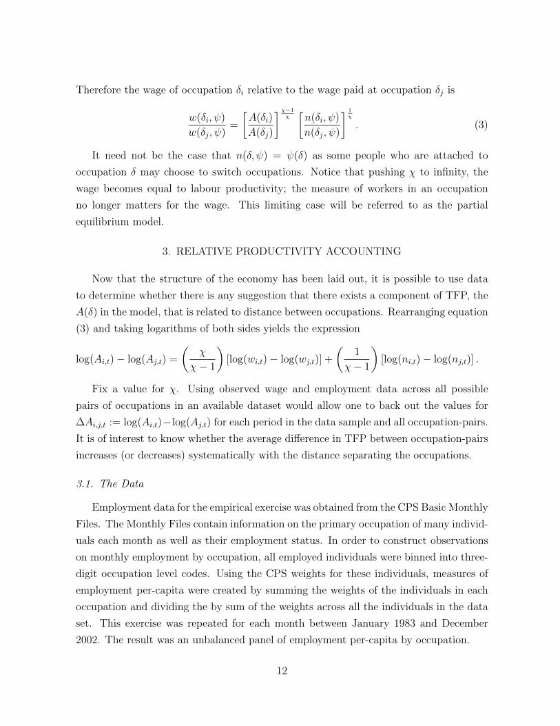
Therefore the wage of occupation δi relative to the wage paid at occupation δj is

w(δi, ψ)

w(δj, ψ)=

[A(δi)

A(δj)

]χ−1χ[n(δi, ψ)

n(δj, ψ)

] 1χ

. (3)

It need not be the case that n(δ, ψ) = ψ(δ) as some people who are attached to

occupation δ may choose to switch occupations. Notice that pushing χ to infinity, the

wage becomes equal to labour productivity; the measure of workers in an occupation

no longer matters for the wage. This limiting case will be referred to as the partial

equilibrium model.

3. RELATIVE PRODUCTIVITY ACCOUNTING

Now that the structure of the economy has been laid out, it is possible to use data

to determine whether there is any suggestion that there exists a component of TFP, the

A(δ) in the model, that is related to distance between occupations. Rearranging equation

(3) and taking logarithms of both sides yields the expression

log(Ai,t)− log(Aj,t) =

(χ

χ− 1

)[log(wi,t)− log(wj,t)] +

(1

χ− 1

)[log(ni,t)− log(nj,t)] .

Fix a value for χ. Using observed wage and employment data across all possible

pairs of occupations in an available dataset would allow one to back out the values for

∆Ai,j,t := log(Ai,t)− log(Aj,t) for each period in the data sample and all occupation-pairs.

It is of interest to know whether the average difference in TFP between occupation-pairs

increases (or decreases) systematically with the distance separating the occupations.

3.1. The Data

Employment data for the empirical exercise was obtained from the CPS Basic Monthly

Files. The Monthly Files contain information on the primary occupation of many individ-

uals each month as well as their employment status. In order to construct observations

on monthly employment by occupation, all employed individuals were binned into three-

digit occupation level codes. Using the CPS weights for these individuals, measures of

employment per-capita were created by summing the weights of the individuals in each

occupation and dividing the by sum of the weights across all the individuals in the data

set. This exercise was repeated for each month between January 1983 and December

2002. The result was an unbalanced panel of employment per-capita by occupation.

12

The panel was unbalanced because there were some occupations that existed in earlier

Census occupation classifications (say the 1980s and 1990s) that were either merged into

other occupation codes in subsequent Census occupation classifications or were elimi-

nated altogether. In order to deal with a balanced panel of occupations, the occupation

classification dataset featured in Dorn (2009) and Autor and Dorn (2013) was used. Fol-

lowing their occupation crosswalk, occupations from the 1980, 1990 and 2000 Census

occupation classifications were merged into a single classification based on the 1990 Cen-

sus occupation classification. The result is a panel of monthly employment shares by

occupation with 330 occupations.12 Taking these time-series, an employment correlation

was constructed for each pair of occupations in the data set.

Earnings data were constructed using the monthly outgoing rotation group files of

the CPS database. For the monthly files between January 1983 and December 2002, each

month, every full-time employed individual was sorted into an occupation and weighted

by their “earnings weight”. The average (weighted) weekly earnings (multiplied by four)

was then calculated for every occupation for every month yielding a panel data set ap-

proximating average monthly earnings per occupation. As there were months in which

some occupations did not register an observation for earnings, all occupations that were

missing at least one observation on earnings were dropped from the panel data set. Using

the remaining 195 occupations, the earnings were matched with per-capita employment

month-by-month to provide a time-series of coupled employment and earnings for each

occupation. Five-month centered moving averages of all earnings and occupational em-

ployment series were used in order to eliminate high-frequency fluctuations.‘’

The objective was to uncover any relationships between relative productivity by

occupation-pairs and the distance between these occupation-pairs. A necessary vari-

able for this exercise was a measure of distance between any occupation pair. Intuitively

if occupations require their workers to perform substantially different tasks then individ-

uals who choose to switch occupations will likely choose to switch between occupations

that require a similar set of tasks. The main reason for this may be to minimize any

loss of task-specific capital if it is the case that wages are tied to such task-specific

capital. Therefore in constructing measures of distance between occupations a data set

containing measures of task-intensity by occupation was required. In order to maintain

12Results spanning January 1983 through December 2009 exhibit similar patterns. However, manyhave noted that there was little change in the Census occupation classifications between the 1980 and1990 classifications while there was some larger changes in between the 1990 and 2000 classificationsystems. For this reason, the results featuring data ending in 2002 are displayed.

13

some comparability to existing work using measures of tasks by occupations, the data

set constructed by Dorn (2009) was utilized as it includes 3-dimensional vectors of task

measures used by each occupation. The task vectors are constructed from data in the

Dictionary of Occupational Titles and are aggregated into three components: Abstract

tasks, Manual tasks and Routine tasks. In using the Dorn measures of tasks, the data on

each task was normalized by subtracting the mean of the task measures (across occupa-

tions) and dividing by the standard deviation of the task measures (across occupations).

This normalization was used because the measures of task intensity preserve order but

their levels cannot be comparable across tasks.

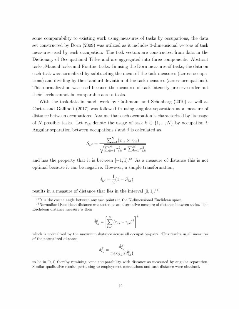
With the task-data in hand, work by Gathmann and Schonberg (2010) as well as

Cortes and Gallipoli (2017) was followed in using angular separation as a measure of

distance between occupations. Assume that each occupation is characterized by its usage

of N possible tasks. Let τi,k denote the usage of task k ∈ {1, ..., N} by occupation i.

Angular separation between occupations i and j is calculated as

Si,j =

∑Nk=1(τi,k × τj,k)√∑N

k=1 τ2i,k ×

∑Nk=1 τ

2j,k

and has the property that it is between [−1, 1].13 As a measure of distance this is not

optimal because it can be negative. However, a simple transformation,

di,j =1

2(1− Si,j)

results in a measure of distance that lies in the interval [0, 1].14

13It is the cosine angle between any two points in the N-dimensional Euclidean space.14Normalized Euclidean distance was tested as an alternative measure of distance between tasks. The

Euclidean distance measure is then

dEi,j =

[N∑

k=1

(τi,k − τj,k)2

] 12

which is normalized by the maximum distance across all occupation-pairs. This results in all measuresof the normalized distance

dEi,j =dEi,j

max(i,j){dEi,j}

to lie in [0, 1] thereby retaining some comparability with distance as measured by angular separation.Similar qualitative results pertaining to employment correlations and task-distance were obtained.

14

3.2. Relative Productivity and Task-Distance

For the accounting exercise a value for χ needed to be selected. Alvarez and Shimer

(2009) argue that in a model of sectoral mobility, elasticities in the range of 2.8 to

4.5 may be reasonable. The model of this paper is not directly comparable to theirs

as the current focus is on occupational mobility and they consider sectoral mobility.

Autor et al. (2008) present a simple model in which college workers and high school

workers work in separate sectors producing intermediate goods via linear production

technologies. These intermediate goods are combined into a final good through use of a

CES production technology. They estimate the elasticity of substitution between the two

types of intermediate inputs to be 1.57. In an attempt to obtain some comparability to

existing work using the Lucas-Island model set-up, the exercise was repeated for elasticity

of substitutions that took on integer values between four and eight. Results for χ = 8

are displayed and the reasons for this choice is explained in Section 4 where the details

concerning the parameterization of the quantitative model are expounded.

For each pair of occupations in the data set, the average of value of the ∆Ai,j,t

across the sample period was calculated, and these averages were binned by the distance

separating the occupation-pairs and plotted in a histogram. In constructing the data on

average distance, let

Ai,j :=1

T

T∑t=1

√(∆Ai,j,t)

2 (4)

which prevents the ordering of Ai and Aj in calculating the distance from mattering.

The left-panel of Figure 2 displays a histogram of these average values, Ai,j, across all

occupation-pairs in the data set.

In order to summarize the relationship between productivity differences and task-

distance, an econometric model was constructed to highlight any pattern that could

be teased out of the histogram. Note that each slice of the histogram, conditional on

distance, resembles a Gamma distribution. Assume that the observations on average

productivity differences, Ai,j, are drawn from a Gamma distribution whose mean and

variance are functions of distance, di,j. A Gamma distribution is characterized by two

parameters, its shape parameter κ, and its scale parameter, ν. The mean of the Gamma

distribution is κν while the variance of the distribution is κν2. Let these parameters

15

Figure 2: TFP Accounting by Distance

depend on distance in the following manner,

κ(d) = exp(φ0 + φ1d+ φ2d2 + ...+ φNΓ

dNΓ)

ν(d) = exp(λ0 + λ1d+ λ2d2 + ...+ λNΓ

dNΓ).

Given a choice for the order of the approximating polynomials, NΓ, a posterior distri-

bution for the parameters {φ0, ..., φNΓ, λ0, ..., λNΓ

} can be estimated. Conditional on this

posterior distribution, the mean of the Gamma distributions can be plotted as distance

is varied. Gather the parameters of the model into a vector Θ = [φ0, ..., φNΓ, λ0, ..., λNΓ

]′

and denote the data collection by Y = {Ai,j, di,j}i,j. According to Bayes’ Rule, posterior

beliefs over Θ, p(Θ|Y), given some priors p(Θ) and some likelihood of observing the data,

p(Y|Θ) is given by

p(Θ|Y) =p(Y|Θ)p(Θ)∫

Θp(Y|Θ)p(Θ)dΘ

,

so that up to a constant,

p(Θ|Y) ∝ p(Y|Θ)p(Θ).

16

Using the Gamma distribution,

p(Θ|Y) ∝∏j 6=i

Γ(Ai,j|κ(di,j), ν(di,j))p(θ).

Ignorance about the values of the parameters was represented by uniform distributions

across each of the parameters to be estimated over a very wide interval, U(−25, 25).15

Additionally, priors over each parameter were chosen to be independent to the priors over

other parameters. An approximation of the posterior distribution was constructed using

a random walk Metropolis-Hasting procedure. The model was estimated for polynomial

lengths NΓ = 1, 2, 3 and the posterior odds ratios revealed that the data preferred a

polynomial length NΓ = 2.16

The right-panel of Figure 2 shows the posterior mean of the Gamma distribution

means (the red line) along with the 95% confidence interval. Of note is the increasing

relationship between the sample mean of TFP differences and the occupational task

distances. It is important to recall that in constructing this empirical accounting exercise,

only the model’s assumptions on production functions along with the assumption that

workers are paid their marginal revenue product were exploited. Nowhere was the model’s

structure on relative productivies imposed. The observation that average relative TFP

between occupations tends to increase with distance suggests that there may be some

merit in the assumption that productivities across occupations may be correlated by the

distance separating them.

4. EMPLOYMENT CORRELATIONS VS TASK-DISTANCE: THE MODEL

This section provides a look at a stark property of the model given the assumptions

on the productivity structure. A quantitative application of the model is presented first

followed by a simple example that highlights the main mechanism at play in the model.

15The realized values for all the parameters were all in a small neighbourhood around zero so the choiceof U(−25, 25) did not play a meaningful role in the results. Initial values for the parameters used toinitiate the random walk Metropolis-Hastings algorithm were found by maximizing the likelihood. Thevariance of the normally distributed innovations to the random walk was adjusted so that approximately30% of the 100,000 draws were accepted.

16The posterior means for the parameters were φ0 = 0.7055, φ1 = 0.1555, φ2 = −0.1355, λ0 = −1.1262,λ1 = 0.2224, λ2 = 0.0472.

17

4.1. Parameterization of the Model

The model is highly stylized and parsimonious in the number of parameters to be

calibrated for the following reason. Several features of the model do not have counterparts

in much of the previous literature so there are no existing values for some parameters

which can be adopted from other work. The solution method is time-consuming and

calibrating the model requires resolving the model several times.17 Thus some functions

are chosen so that there are minimal parameters while retaining some intuitive appeal.

The two functions that are most model-specific are the function representing the levels

of TFP across occupations, g(δ), and the function representing the distibution of shocks

to the location of the g(·) function’s mode. For simplicity, the g(·) function is represented

by a symmetric Beta p.d.f. function. This choice means that there is a single parameter

governing the shape of the TFP function which can be bell-shaped or strictly concave

down. Both these shapes allow the most productive occupation to be centered in the

domain [−π, π] and are uni-modal. Let ξ represent the parameter governing the shape of

the TFP function. TFP in the most productive occupation is normalized to a = 1 and

the level of TFP in the least productive occupation is a.

As the shocks must be confined to lie in a circle, the (symmetric) Beta distribution

was chosen to govern the reallocation shock process. The Beta distribution has a domain

[0, 1] so this interval was stretched into [−π, π] using a linear change-in-variables. Given

the symmetry assumption, these shocks then have a mean of zero so that the identity of

the most productive occupation follows a Martingale process. Again, this choice allows

the shock process to be summarized by a single parameter, αε.

The parameters governing the productivity process were chosen in an effort to reflect

the findings from the productivity accounting exercise. A set of parameters, {a, ξ, αε, σ2e},

was picked where σ2e is the variance of a mean zero Normal distribution from which

“measurement error” would be drawn. As is discussed in the following, this measurement

error helped parameterizations of the shock process to fit the red line in the right-panel

of Figure 2. Given values for this set of parameters, a time series for the location of the

mode, {θt}Nsimt=0 , was simulated, with Nsim = 5000 being the number of periods in the

simulation. For each of these Nsim periods the TFP for occupations in a discrete number

17See Appendix for a detailed description of the solution method. While the partial equilibrium modelcan be solve within seconds, the general equilibrium model takes anywhere from several minutes to manyhours, depending on the elasticity of subsitution and the quality of initial guesswork for the equilibriumfunctions.

18

nocc of evenly-spaced occupations around the circle of radius one was constructed.18 This

yielded a simulated panel of data for TFP across a large number of occupations. With

this simulated panel-data in hand, for each pair of occupations, say i and j, a mean

TFP-distance, Ai,j, was calculated following equation (4).

Next, each of Ai,j constructed in the simulation, was multiplied by a “measurement

error” term to construct a set of observations

A∗i,j = Ai,j exp(ei,j), ei,j ∼ N(0, σ2

e).

Finally the set {A∗i,j} was sorted by the minimum distance between each pair i and j

around the circumference of the unit circle. Let D :={di,jπ

: i, j ∈ {1, ..., nocc}}

be the

set of all normalized distances between occupation-pairs that appear in the simulated

data set. The average of the A∗i,j for each distance d ∈ D was constructed as

ζχ(d) =

(1

Nd

) ∑di,j=d

A∗i,j.

Note that ζχ(d) is conditional on a value of χ as constructed values of A∗i,j are dependent

on the chosen value for χ.

Denote the estimated relationship linking occupation-pair productivity differences

and occupational distance (as illustrated in the right-panel of Figure 2) by ζχ(d). Let the

simulated analogue of the estimated relationship be given by ζχ(d). For a given elasticity

parameter, χ, the parameters {a, ξ, αε, σ2e} were chosen to minimize the sum of squared

distances,

D(χ) = min{a,ξ,αε,σ2

e}

{1

2

∑d∈D

(ζχ(d)− ζχ(d)

)2}.

In order to select a value for χ, the parameter fitting exercise was repeated for integer

values of χ from four to eight. The value of χ = 8 was selected for results presen-

tation in this paper because at this elasticity, the difference between the fitted TFP

correrlation-distance relationship and that estimated relationship was minimized (that

is, argminχ∈{4,5,6,7,8}D(χ) = 8).19

18For the exercise presented nocc = 201.19While the fit generated by the parameterization at χ = 8 is striking, the fit at all values of χ ∈{4, 5, 6, 7, 8} generated simulated relationships that mainly laid in the 90% interval from the estimatedrelationship. The estimated relationships across the various values of χ were similar in shape as thedisplayed results for χ = 8.

19

Figure 3: Parameterizing the Reallocation Shock Process

Fitted values for {a, ξ, αε, σ2e} are listed in Table 1 and the fit is illustrated in the

left-panel of Figure 3. The upper-right and lower-right panels in Figure 3 depict the

TFP function and the distribution for the aggregate reallocation shocks that are derived

from this parameter fitting exercise. The fitted value for the variance of the measurement

errors is σ2e = 0.1876. Measurement errors were added to the exercise to allow the level

of the fitted function in the left-panel of Figure 3 to match its target. In other words,

the presence of the measurement error shifts the intercept of the fitted function while

the shape of the fitted function derives mainly from the parameters, a, ξ, and αε. As the

focus of this paper is on the role of aggregate reallocation shocks, the shape of the fitted

function is of greater interest than the levels. The model features only a single type of

shock so if similar occupations are to experience similar TFP fluctuations, then there is

little hope in the model for similar occupations to have wildly different levels of TFP.20

Table 1 displays the values used for the various parameters in the quantitative exercise.

In order to abstract from issues of risk-aversion a linear utility function, u(c) = c, was

employed. As there is no saving in the model, adding risk-aversion would result in an

20Adding a persistent, occupation-specific TFP component that is independent across occupationswould create much more disperion in occupational TFP and suppress the need of measurement error.However, from the modelling perspective this component would put the problem back to tracking a jointdistribution of employment and TFP across occupations.

20

Table 1: Parameter Values

Parameter Value Descriptionβ 0.9976 Subjective discount factorχ 8 Elasticity of substitution in final goods CES aggregatora 0.2762 Lower bound for labour productivitya 1 Upper bound for labour productivityξ 1.8467 Shape parameter for labour productivity function g(δ)αε 1957 Parameter governing distribution of shocksµz 5 Mean of idiosyncratic shocks from Gamma Distributionσ2z 11 Variance of idiosyncratic shocks from Gamma Distributionb 0.3 Fraction of lowest wage consumed by occupation switchersη 375 Weight on quadratic retraining cost

occupational wealth property in occupational choice which could obscure the main results

to be depicted. As the data used in the empirical work was at a monthly frequency, the

discount factor, β, was chosen so that workers expect to participate in the labour force

for 420 months (or 35 years). When not employed, individuals enjoy consumption in the

amount cb = bminδ w(δ) where minδ w(δ) is the lowest wage paid in the economy within

the period. The idea of b is to act as a loose approximation to a replacement ratio.

The distance related cost function of switching occupations ϕ(x) is represented by a

simple quadratic function η2x2. The value of η was chosen in conjunction with the pa-

rameters governing the distribution of fixed costs, H(z), that is represented by a Gamma

function with mean µz and variance σ2z .

21 In parameterizing the triple (η, µz, σ2z),

a calibration procedure targetted an average (monthly) occupational mobility rate in

the neighbourhood of 1.7% along with a sample correlation for detrended real GDP per

worker with its own lag of 0.91 and a standard deviation for output per worker of 0.0117.22

The argument for a monthly occupation switching rate of 1.7% is that if each month,

individuals are randomly selected to switch occupations with equal probability, then the

annual occupational switching rate would be 18.5%. In their calculations of occupational

switching rates, Kambourov and Manovskii (2009), show that occupation switching rates

21Given the choice of µz and σ2z , it is easy to reverse engineer the Gamma distribution parameters

that correspond to this mean and variance.22In calculating the statistics for real GDP per worker, U.S. data for quarterly real GDP and quarterly

averaged total employmend between 1983Q1 and 2002Q4 was used. After calculating quarterly loga-rithms for real GDP per workers, a linear trend was extracted that minimized the Euclidean distancebetween the linear trend and the sample data. This resulted in a fitted intercept and growth rate forwhich the linear trend was constructed.

21

Table 2: Simulated Ensemble Results

Percentiles: 5th 17th 83rd 95th Mean Target

Monthly Switching Rate 0.0116 0.0125 0.0208 0.0271 0.0167 0.017Ave Persistence of Output Per Worker 0.7870 0.8504 0.9511 0.9680 0.8998 0.91Ave Volatility of Output Per Worker 0.0026 0.0041 0.0135 0.0183 0.0088 0.0117

in the U.S. ranged from 16% in the late-1970s to as high as 21% in the mid-1990s.

In order to accomplish this calibration task, the model was solved using a set of

parameter values and then simulated to produce an ensemble of time-series of size Nsim

such that each time-series in the ensemble contained 240 periods which is the length

of the data set used in the empirical work in this paper. For each time-series in the

ensemble, the average monthly occupation switching rate, the first-order autocorrelation

and the standard deviation for quarterly output per worker were calculated. This yielded

a ensemble distribution for each of these statistics. Table 2 provides some information

concerning the distribution of the ensemble statistics produced by this procedure using

the parameters shown in Table 1.

4.2. A Testable Implication of the Model

The property of the model that is the focus of this paper is the average correlation of

employment between occupation-pairs relative to the distance between them. In order

to get a feel for the model’s implication, the model was simulated for 15000 periods and

for each period, the distribution of employment and occupational TFP across a large

set of occupations (151 occupations in total on a uniformly-spaced grid of [0, 2π]) was

stored. The first 5000 periods of the simulation were then dropped. Given this data,

employment correlations were then calculated across all possible occupation-pairs and

occupation-pairs were binned by distance using a large set of distance bins (distances

between 0 and π).

The take-away from Figure 4 is that the model produces a negative relationship be-

tween employment-correlation and distance separating occupation-pairs. The red line

in Figure 4 plots the average employment correlations between occupation-pairs sorted

by distance (normalized so that the maximum distance is one) while the shaded region

represents the employment correlations covered by the [5,95] percentile interval condi-

tional on distance. The blue line plots the correlation of occupational TFP by distance.

22

Figure 4: G.E. Model: Distance Vs Employment Correlations

Note that the blue line lies in the 90% interval of the employment-distance relationship.

This implies that at the elasticity of substitution of χ = 8, the general equilibrium forces

are not sufficiently strong enough to generate endogenous employment correlations by

distance that are different than the exogenous TFP correlations by distance. Although

the general equilibrium model does feature some complementarity between intermediate

inputs, the general equilibrium pressures on wages are not large with χ = 8. By taking

the logarithm of equation (3), it is surmised that the general equilibrium effect of relative

employment on relative wages only gets large with χ approaching two or three.

The observation that the occupational employment correlation is systematically re-

lated to occupational distance is a qualitative property of the model. The observation

that this relationship is strictly decreasing is conditonal on the fitted productivity pro-

cess. In the following section it is shown that the correlated occupational TFP structure

is the responsible for the systematic relationship between employment correlations and

distance.

23

4.3. A Simple Example

The novelty of this model is that it provides a tractable framework that can be

solved quantitatively to study general equilibrium dynamics of an economy with many

occupations in which the wage function is allowed to be determined as an equilibrium

object. In order to achieve this, it is assumed that productivities across occupations are

correlated as a function of the distance between the occupations. This stands in contrast

to a standard assumption imposed in applications of the Lucas-Prescott island model

that productivity processes across islands are independent.

In order to highlight the contribution of the correlated occupational TFP assump-

tion, this section contrasts the equilibrium results to that of a similar economy in which

occupational total factor productivity processes are independent across islands.23 To

keep the argument as transparent as possible, consider an example in which occupational

outputs are perfect substitutes. This is the partial equilibrium case of the production

structure discussed in the more general model with χ, the elasticity of substitution in

the CES production function, pushed towards infinity. Retaining the assumption of free

entry into job creation and perfect competition, real wages are equated to occupational

TFP. Additionally, assume that individuals face an exogenous probability of being able

to switch occupations and individuals who choose to switch occupations are randomly

allocated to new occupations at the end of the current period with uniform probability;

in time to experience the new occupation’s productivity shock at the beginning of the

next period.24 Assume that the productivity function features the same properties in the

general equilibrium model with endogenous switching decisions; it is symmetric around

zero, unimodal, with productivity strictly decreasing with distance from the mode and

defined on the interval [−π, π]. Finally, retain the assumption that the probability of oc-

cupational TFP shocks are decreasing (symmetrically) with the size of the shocks. This

model will be referred to as the Simple Model.

Under the random reallocation assumption, individuals face the same continuation

value when switching occupations. As productivity is symmetric around the mode and

strictly decreasing with distance from the mode there are cut-off occupations associated

with a cut-off distance, such that occupations that are farther than the cut-off distance

from the mode feature endogenous outflows of individuals while those close enough to

23For a detailed description see the Appendix.24Examples of work using the assumptions of random assignment amongst island switchers along with

independent island TFP processes include Veracierto (2008) and Alvarez and Shimer (2009).

24

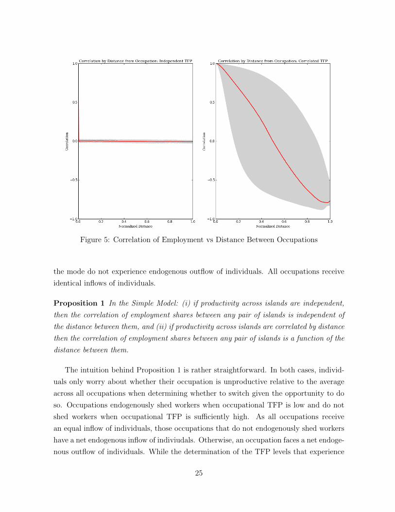
Figure 5: Correlation of Employment vs Distance Between Occupations

the mode do not experience endogenous outflow of individuals. All occupations receive

identical inflows of individuals.

Proposition 1 In the Simple Model: (i) if productivity across islands are independent,

then the correlation of employment shares between any pair of islands is independent of

the distance between them, and (ii) if productivity across islands are correlated by distance

then the correlation of employment shares between any pair of islands is a function of the

distance between them.

The intuition behind Proposition 1 is rather straightforward. In both cases, individ-

uals only worry about whether their occupation is unproductive relative to the average

across all occupations when determining whether to switch given the opportunity to do

so. Occupations endogenously shed workers when occupational TFP is low and do not

shed workers when occupational TFP is sufficiently high. As all occupations receive

an equal inflow of individuals, those occupations that do not endogenously shed workers

have a net endogenous inflow of indiviudals. Otherwise, an occupation faces a net endoge-

nous outflow of individuals. While the determination of the TFP levels that experience

25

outflows in each period is endogenous in the aggregate, the identity of the occupations

shedding workers depends only on whether or not that occupation’s TFP lies below a

threshold TFP level. Under independence of TFP processes, occupations that currently

shed individuals do so irrespective of the outcomes in nearby occupations because TFP

is not related to TFP in nearby occupations. By constast, consider an economy in which

the time-series properties of TFP for each occupation mirrors that of the independent

TFP case with the only difference being that TFP across occupations is correlated by

distance. In this case, when a given occupation’s TFP lies below the TFP threshold it

is highly likely that nearby occupations also have occupational TFP that lies below the

threshold for switching. In this case, occupations that are close to each other tend to

shed individuals simultaneously.

Figure 5 provides the correlations between employment and distance in such a partial

equilibrium example with random reallocation.25 The left-panel shows the case in which

occupational TFP processes are identical and independent. Occupation-pairs separated

by distances greater than zero all feature similar correlations. For comparison, the right-

panel plots employment correlations versus distance between occupation-pairs in the

economy where TFP between occupations is correlated by distance. By construction,

from the perspective of any given occupation, the dynamics of the TFP processes are

identical between the two examples and individuals in both economies have identical

value functions and decision rules. This highights the effects of correlating TFP by

distance between occupations and the potential that such a rather intuitive structure on

productivity has to help understand the employment flows that are observed in the data.

Thus the model provides a simple environment in which employment correlations

across occupation-pairs are related to the distance separating them. The following section

roots around the U.S. labour market data to see if such a relationship exists.

5. EMPLOYMENT CORRELATIONS VS TASK-DISTANCE: THE EMPIRICS

Given the implications arising from the assumptions concerning frictional reallocation

across occupations and the properties of the aggregate reallocation shock structure, the

employment and task data from Section 3 is reexamined to determine whether there is a

notable relationship between employment correlations between occupation-pairs and the

25In constructing Figure 5 the productivity processes were identical to that in the general equilibriummodel and the probability of switching was chosen to yield a switching rate of 1.7% per period.

26

Figure 6: Employment Correlations vs Distance: Using Angular Separation

distance that separates them.26

After constructing measures of distances between occupation-pairs, and correlation of

employment between each occupation pair, a simple econometric model was used to tease

out any relationship between distance and employment correlation. Figure 6 displays all

the data used in the econometric exercise. The left-panel is a three-dimensional plot of

the histogram of employment correlations as the distance between occupation-pairs is

varied. The right-panel provides a contour plot of the data. As can be seen there is

much variance in employment correlations conditional on each value of distance. Part of

this variance is likely due to approximation noise in constructing employment per-capita

by occupation using monthly CPS data files as some occupations only consist of one or

two observations per month which are then used to provide an approximation to the

aggregate number of individuals employed by the given occupation in the population.

Given a data set consisting of N employment correlation-distance pairs, the objective

was to estimate a model relating the employment correlation between two occupations

to the distance between the occupations. In order to do so, it was assumed that the

26As earnings data was not required for this exercise, I used employment data from all 330 occupationsin the Dorn (2009) dataset to construct the pairwise employment correlation data as well as the task-distances following the procedures outline in the previous sections.

27

correlation between two occupations that are a distance d from each other were drawn

from a Beta distribution with a mean and variance that were dependent on the value of

d. The reason for this modelling choice was that each cross-section of the histogram in

Figure 6 conditional on distance looked like it could be a sample from a Beta distribution

which is a simple two parameter distribution that has a support given by [0, 1].

Employment correlations take values in the interval [−1, 1] and normalized distances

belong to the interval [0, 1]. Let the distance between occupations i and j be denoted

by di,j and the correlation of employment between the two occupations be denoted by

ρi,j. Suppose ρi,j is drawn from a Beta distribution B(α, β). As the support of the Beta

distribution is the interval [0, 1], a simple change-of-variables ρi,j =ρi,j+1

2was used so

that the transformed correlations ρi,j lie in the interval [0, 1].

In an effort to permit flexibility in the correlation-distance relationship, the parame-

ters of the Beta distribution were modelled as functions of the distance between occupa-

tions. In order to accomplish this, consider the following functions

µ(d) = ϕ0 + ϕ1d+ ϕ2d2 + ...+ ϕnd

nα , (5)

σ(d) = η0 + η1d+ η2d2 + ...+ ηnd

nβ . (6)

These two functions were meant to capture the effects of distance on the mean and

variance of the Beta distribution. Here nα is the order of the approximating polynomial

µ(d) and nβ is the order of the approximating polynomial σ(d). Letting µ and σ2 represent

the mean and variance of the Beta distribution, I used the mapping,

µ(d) =exp(µ(d))

1 + exp(µ(d))

to obtain a mean in the interval (0, 1) and the mapping

σ2(d) =1

4

[exp(σ(d))

1 + exp(σ(d))

]to ensure that the variance lies in the interval (0, 0.25). Note that this allows the mean

and variance of the Beta distribution to vary with distance.

Given a feasible pair (µ, σ2) the parameters of the Beta distribution are retrieved as

α(d) =(1− µ(d))µ(d)2 − µ(d)σ2(d)

σ2(d)

and

β(d) = α(d)

(1− µ(d)

µ(d)

).

28

As the Beta distribution is defined on a domain of [0, 1], the estimated Beta distribu-

tion mean on the random variable ρ ∈ [0, 1] can be mapped back into the interval [−1, 1]

(in which the true correlations lie) by a simple linear transformation27

µb(d) = 2µ(d)− 1.

Gather the parameters of the model into a vector θ = [ϕ0, ..., ϕnα , η0, ..., ηnβ ]′ and

denote the data collection by y = {ρi,j, di,j}i,j. Using the Beta distribution, following

Bayes’ Rule, the posterior distribution is such that

p(θ|y) ∝∏j 6=i

B(ρi,j|α(di,j), β(di,j))p(θ).

Again, ignorance over the values of the parameters in the statistcal model are repre-

sented by uniform distributions over each of these parameters over a very wide interval,

U(−25, 25). Additionally, priors over each parameter are independent to the priors of

other parameters. An approximation of the posterior distribution was derived using a

random walk Metropolis-Hasting procedure.

5.1. Results

In constructing the empirical estimates using angular separation as a measure of dis-

tance, several versions of the model were estimated differing by the order of polynomials

used in equations (5) and (6) starting with third-order polynomials in both the mean

and variance equations and paring down to first-order polynomials. The posterior odd

ratios suggested that the data preferred the version of first-order polynomials to models

using second- or third-order polynomials in both equations.28

The left-panel in Figure 7 displays the estimated relationship beween employment-

correlations and distance between occupation-pairs. The red line plots the mean of the

correlations as a function of distance constructed from the estimated posterior distribu-

tion over the model parameters while the grey region covers the 95% confidence interval

of the function. The right-panel displays a plot of the posterior mean of the estimated

correlation-distance relationship over the contour plot of the data histogram. This plot

shows how the posterior mean follows a ridge in the joint distribution of the correlation-

distance data.29

The main feature to highlight from the econometric exercise is that there appears to

be a clear, negative relationship between employment correlations and distance between

27The variance of the random variable ρ ∈ [−1, 1] can be calculated using the estimated Beta distri-

29

Figure 7: Employment Correlations vs Distance: Using Angular Separation

occupations. While there is obviously much variation in this data conditional on distance,

this is likely to be expected given the number of shocks that can be thought of as buffeting

the labour markets in the aggregate, at the industry level, across geographical regions,

etc.

The empirical results suggest that there may be some merit to assuming some distance-

related correlation in productivity experienced at the occupation level. The model in this

paper has only featured a single type of shock, mainly for reasons related to minimizing

computational complexity.

5.1.1. Results for the Standard 3-Bin Classification System

The recent literature on occupational mobility has emphasized the hollowing out of

employment in the routine-manual tasks. Specifically, this literature has shown that over

the course of the last three decades employment has shifted from occupations exploiting

bution parameters (α(d), β(d)) and the linear change-of-variables ρ = 2ρ− 1.28The posterior means of the parameters were ϕ0 = 0.2540, ϕ1 = −0.4479, η0 = −1.5097, η1 = 0.0047.29The point estimates of a simple OLS regression of employment correlations on a set of regressors

comprised of first-, second- and third-order polynomials looks extremely similar to the plotted mean con-structed of the posterior distribution. However, the OLS model is not constrained to produce estimatesthat respect the maximum and minimum feasible correlations.

30

Figure 8: Employment Correlations vs Distance: The 3-Bin Classification System

routine manual (RM) tasks to those requiring either non-routine cognitive (NRC) or

non-routine (NRM) manual tasks. Examples of such work include Autor et al. (2003),

Acemoglu and Autor (2010), Jaimovich and Siu (2012), and Cortes (2016) amongst many

others. From this literature, it may not surprising that employment-correlations appear

to decrease with distance between occupational tasks.

In order to see whether the negative relationship between employment correlation and

task-distance is mainly driven by occupation-pairs that lie across separate bins in the 3-

Bin classification system, the econometric exercise was repeated separately by first sepa-

rating the 3-digit occupations into the three task bins; routine manual, non-routine man-

ual and non-routine cognitive using the classification tables provided in Cortes (2016).

Using the same econometric model as describe in Section 5, the relationship between em-

ployment correlation and task distance for occupation-pairs that belonged to the same

task classifications were estimated first. These results are shown in the top row of Fig-

ure 8 while the bottom row displays the results from estimating the results using only

occupation-pairs that lie across two occupation classification bins.

Each plot in Figure 8 displays the results with the red lines plotting the posterior

31

Table 3: Ave (Angular Separation) Distance Between Occupations within Categories

Occupation-Type NRC NRM RM

NRC 0.358 0.593 0.604NRM - 0.276 0.485RM - - 0.406

Note: Occupation-types are partitioned into Non-Routine Cognitive (NRC), Non-RoutineManual (NRM) and Routine Manual (RM).

means and the shaded-grey regions being the 95% confidence intervals. The lighter-

grey regions represent the distances within which the lowest and highest 10% of the

data lie while the intermediate darker-grey region shows the region in which the middle

80% of the observations (ordered by distance) lie. The dashed line signifies the mean

distance of all the observations within the sample used to estimate the model and their

numerical values are given in Table 3. Figure 8 shows that the negative relationship

between employment correlations and task-distances obtained when using the full sample

are likely driven by the relationships between occupation-pairs completely housed in the

non-routine cognitive classification, completely housed in routine manual classification

or spread between non-routine cognitive and routine manual classifications. All three of

these plots (top-left, top-middle and lower-right panels) show a clear negative relationship

between employment correlations and task-distances. Note that the slopes are clearly

negative at the mean task-distances of the sample used in each estimation exercise (i.e.

the slopes are negative when intersecting the dashed lines). Also note that the magnitude

of change from the maximum to the minimum in each of these plots is substantial in

relation to the difference between the maximum and minimum when using the entire

data set as shown in Figure 7. The estimates are less precise when using non-routine

manual occupations as these are the fewest in number.

Summarizing the empirical observations, it appears as though, on average, employ-

ment correlations of occupation-pairs are decreasing as their task-distances increase. Fur-

thermore, this observation is not only present in the panel of all occupations but also

exists when looking within occupation-pairs belonging to each of the standard 3-Bin

classifications. This suggests that when looking at such dynamic relationships across

occupations, it may be useful to have a model that involves a more granular view of

occupational change along with some notion of distance between occupations.

32

6. CONCLUSION

The model presented in this paper has provided a novel framework within which to

think about the effects of shocks to occupations which are linked by the task-distance that

separates the occupations. Given a productivity structure that links occupational TFP

differences to relative task-distances between occupations, a stark implication arose that

occupational employment correlations between any two occupations should be related to

their task-distance. An empirical exploration of U.S. labour market data revealed that

a negative relationship exists between the correlation of employment across occupations

and the task-distance that separates these occupations.

A contribution of the model to the existing literature on labour reallocation is that

it enables an explicit examination of labour market dynamics in a general equilibrium

setting with aggregate shocks and many distinct labour markets. As a main implication

of the model appears to be supported by employment data, researchers can be more

confident in adopting and upgrading the model to study the general equilibrium dynamics

of wage inequality, labour reallocation and issues related to trade-offs between retraining

subsidies and unemployment insurance at the aggregate level.

33

APPENDIX A. EMPLOYMENT CORRELATIONS: A SIMPLE MODEL

Consider the partial equilibrium model (perfect substitution of intermediate goods in

the final goods sector) without distance costs. In this case, w(i) = A(i). Furthermore,

for simplicity, assume that workers who switch islands are randomly allocated to a new

island with equal probability across all islands and each period, an individual faces an

exogenous probability λ of being able to switch islands. Also, assume that for each island

i, A(i) follows a Martingale process with the identity of the productivity frontier NOT

being uniformly distributed across occupations. Finally, retain the assumptions that

occupational TFP is decreasing (symmetrically) in distance from the productivity frontier

and that the probability of occupational TFP shocks are decreasing (symmetrically) with

the size of the shocks.

Proposition #1: In the Simple Model: (i) if productivity across islands are indepen-

dent, then the correlation of employment shares between any pair of islands is indepen-

dent of the distance between them, and (ii) if productivity across islands are correlated

by distance then the correlation of employment shares between any pair of islands is a

function of the distance between them.

Proof : Case #1: First fix some notation. Partition the interval [0, 2π] into 2N∆ + 1

bins of width ∆. Index this set of bins by LBG := {1, 2, ..., 2N∆ + 1} with the set of bin

edges denoted by LEG = {0,∆, 2∆, ..., 2π}. Denote the location of occupation i in the set

of bins LBG by

li := max{n ∈ LBG : (n− 1)∆ = max{l ∈ lEG : l ≤ i}}.

Define the distance between occupations j and k, with j, k ∈ [0, 2π] (in units of LBG bins)

by

dj,k := min {max{lj, lk} −min{lj, lk},min{lj, lk} −max{lj, lk}+ (2N∆ + 1)} .

Next, consider a grid of 2N∆ + 1 evenly-spaced bins of width ∆ indexed by elements

of the set ∆BG := {−N∆,−N∆ + 1, ..., 0, ..., N∆ − 1, N∆} (the grid of bins) with a set of

2(N∆ + 1) accompaying bin edges denoted by ∆EG := {−π,−π + ∆,−π + 2∆, ...,−π +

N∆∆,−π + (N∆ + 1)∆, ..., π}. Also, create a set of bins by partitioning [−π, π] into

(2N∆ + 1)α bins, α ∈ N begin a natural number. Denote the this set of (2N∆ + 1)α bins

by δBα and let δEα denote the set of (2N∆ + 1)α + 1 edges of the bins in δBα . This permits

34

each occupation i ∈ [0, 2π] to be assigned to a unique bin in δBα first by transforming

i ∈ [0, 2π] to i ∈ [−π, π] following

i =

{i if i ∈ [0, π]i− 2π if i ∈ [π, 2π],

and then finding δ(i) ∈[min{j ∈ δEα : j ≥ i} − 2π

(2N∆+1)α,min{j ∈ δEα : j ≥ i}

]. The val-

ues δ(i) can then be mapped into the bins belonging to ∆BG by first determining the

n ∈ {1, ..., 2N∆ + 1} such that δ(i) ∈ [−π + (n− 1)∆,−π + n∆] and using n to identify

the nth element of ∆BG. This mapping from i into ∆B

G provides a way to assign an initial

condition to each i in terms of bins in ∆BG. To reduce notation, from here onwards let

∆i denote the bin of ∆BG to which an occupation i is assigned.

Over time, occupations are reassigned between bins in the set ∆BG. Define the set of

possible shocks as ∆ε := {−N∆∆,−(N∆ − 1)∆, ..., 0, ..., (N∆ − 1)∆, N∆∆} so that there

are 2N∆ + 1 elements in ∆ε. As each shock in ∆ε is a multiple of ∆, we can index the

shocks by the size of the multiple which are gathered in the set ∆Mε := {−N∆,−(N∆ −

1), ..., 0, ..., N∆ − 1, N∆}. Note that ∆Mε = ∆B

G. The probability of a given shock, ε ∈ ∆ε,

being drawn is denoted by π(ε) with draws being independent across time and between

occupations. Thus the reallocation of occupations across bins in ∆BG is summarized by

∆′i =

∆i + ε

∆if ∆i + ε

∆∈ ∆B

G

∆i + ε∆

+ (2N∆ + 1) if ∆i + ε∆< −N∆

∆i + ε∆− (2N∆ + 1) if ∆i + ε

∆> N∆.

(A.1)

The probability of drawing shocks, π(ε) together with the transition equation (A.1) results

in a conditional distribution for ∆ denoted by F (∆′|∆). Assume that π(ε) is symmetric

with respect to |ε| and that π(ε′) > π(ε′′) if |ε′| < |ε′′|.Let the productivity of an island be a function of its bin ∆i ∈ ∆B

G so that produc-

tivity of island i is A(∆i). Consider a continuous and increasing function, A : ∆BG →

[0, Amax] (for finite Amax), with argmax∆∈∆BGA(∆) = ∆0, argmin∆∈∆B

GA(∆) = ∆N∆

and

A(∆N∆) = 0. Also assume that for i, j ∈ {−N∆,−N∆ + 1, ...,−1, 0, 1, ..., N∆ − 1, N∆},

A(∆i) > A(∆j) if |i| < |j|, and, for simplicity, impose symmetry so that A(∆i) = A(∆j)

if |∆i| = |∆j|.Each period, an individual has a probability λ of being able to switch occupations.

Otherwise, the individual has no other option but to work for the prevailing wage in

his/her current occupation. In switching occupations, individuals receive no consumption

35

in the current period. For any ∆ ∈ ∆BG, the value of switching from any island is

T (∆) = β

∫ π

−π

∫ π

−π{λmax [T (∆′), V (∆′)] + (1− λ)V (∆′)} dF (∆′|∆∗)dU(∆∗).

subject to

∆′ =

∆∗ + ε

∆if ∆∗ + ε

∆∈ ∆B

G

∆∗ + ε∆

+ (2N∆ + 1) if ∆∗ + ε∆< −N∆

∆∗ + ε∆− (2N∆ + 1) if ∆∗ + ε

∆> N∆.

(A.2)

Notice that the value of switching occupations is identical for all current period ∆ so we

can indicate the value of switching by T ∗. Rewriting,

T ∗ = β

∫ π

−π

∫ π

−π{λmax [T ∗, V (∆′)] + (1− λ)V (∆′)} dF (∆′|∆∗)dU(∆∗). (A.3)

subject to (A.2).

The value of employment in an occupation satisfies

V (∆) = A(∆) + β

∫ π

−π{λmax [T ∗, V (∆′)] + (1− λ)V (∆′)} dF (∆′|∆). (A.4)

subject to

∆′ =

∆ + ε

∆if ∆ + ε

∆∈ ∆B

G

∆ + ε∆

+ (2N∆ + 1) if ∆ + ε∆< −N∆

∆ + ε∆− (2N∆ + 1) if ∆ + ε

∆> N∆.

(A.5)

where T ∗ has been subsituted for T (∆′).30

In order to see that there is a solution to the individual’s problem, note that V (∆) and

T ∗ are bounded from below by zero and from above by Amax1−β . Let equations (A.3) and (A.4)

define a mapping (V j+1, T ∗j+1) = M(V j, T ∗j). Consider the space of bounded functions

endowed with the sup-norm. It can be shown that Blackwell’s sufficient conditions for a

contraction are met so that there exists a fixed point (V, T ∗) = M(V, T ∗).

Next it is shown that V (∆) is non-increasing in |∆|. Let the expected continuation

return be given by

R(∆) =

∫ π

−π{λmax{τ, v(∆′)}+ (1− λ)v(∆′)} dF (∆′|∆)

=

2N∆+1∑i=1

f(∆′i|∆) {λmax{τ, v(∆′i)}+ (1− λ)v(∆′i)}

30Notice that if π(ε) follows the uniform distribution then it is never optimal to switch occupations.This case is is ignored as it is uninteresting.

36

with the transition equation for ∆ given by (A.5). Let v(∆) be a non-increasing function

in |∆|. First show that R(∆) is non-increasing in |∆|. Clearly, the term λmax{τ, v(∆)}+(1− λ)v(∆) is non-increasing in |∆| given the assumed property of v(∆).

Consider the difference

R(∆∗)−R(∆) =

2N∆+1∑i=1

(f(∆′i|∆∗)− f(∆′i|∆)) {λmax{τ, v(∆′i)}+ (1− λ)v(∆′i)} . (A.6)

It will be shown that this difference is non-negative if ∆∗ ∈ [−π, 0] and |∆∗| < |∆|.First suppose that ∆∗ ∈ [−π, 0] and ∆ ∈ [−π,∆∗]. Find the bounds [∆L,∆U ] such

that f(∆′i|∆∗) ≥ f(∆′i|∆). By symmetry, for every ∆′i ∈ [∆L,∆U ] there is a ∆′i ∈[−π,∆L] ∪ [∆U , π] such that f(∆′i|∆∗) − f(∆′i|∆) = f(∆′i|∆) − f(∆′i|∆∗) with v(∆′i) >

v(∆′i). Therefore, in such cases, the difference in equation (A.6) is non-negative. The

left-panel of Figure 9 provides an illustration of such a case.

Similarly, suppose that ∆∗ ∈ [−π, 0] and let ∆ ∈ [−∆∗, π]. Again, define ∆L and

∆U such that for all ∆′i ∈ [∆L,∆U ], there is a ∆′i ∈ [−π,∆L] ∪ [∆U , π] with f(∆′i|∆∗)−f(∆′i|∆) = f(∆′i|∆) − f(∆′i|∆∗) and v(∆′i) ≥ v(∆′i). An example of such a case is

illustrated in the right-panel of Figure 9. In such cases, the difference in equation (A.6)

is non-negative. Thus for any value of ∆∗ ∈ [−π, 0] it is the case that if |∆∗| < |∆|, the

difference in equation (A.6) is non-negative.

It is straightforward to flip the previous reasoning around to show that the difference in

equation (A.6) is non-increasing in |∆| for ∆ ∈ [0, π]. Take the cases in which ∆∗ ∈ [0, π]

and ∆ ∈ [−∆∗, 0]. Find the bounds ∆U and ∆L such that ∆U < ∆ < ∆L < ∆∗ with

f(∆′i|∆) ≥ f(∆′i|∆∗) for ∆′i ∈ [∆U ,∆L]. For every ∆′i ∈ [−π,∆U ] ∪ [∆L, π], there is a

∆′i ∈ [∆U ,∆L] such that f(∆′i|∆∗)− f(∆′i|∆) = f(∆′i|∆)− f(∆′i|∆∗) and v(∆′i) ≥ v(∆′i).

For these cases, the difference in equation (A.6) is non-positive.

The last step to show that the difference in equation (A.6) is non-increasing for ∆ ∈[0, π] is to consider the cases in which ∆∗ ∈ [0, π] and ∆ ∈ [0,∆∗]. Find the bounds

∆U and ∆L such that f(∆′i|∆) ≥ f(∆′i|∆∗) on the interval [∆U ,∆L]. Then for every

∆′i ∈ [−π,∆U ] ∪ [∆L, π] there is a ∆′i ∈ [∆U ,∆L] such that f(∆′i|∆∗) − f(∆′i|∆) =

f(∆′i|∆)−f(∆′i|∆∗) and v(∆′i) ≥ v(∆′i). Again, for these cases, the difference in equation

(A.6) is non-positive. Then for any value of ∆∗ ∈ [0, π] it is the case that if |∆∗| >|∆|, the difference in equation (A.6) is non-positive. Hence, the function R(∆) is non-

increasing in |∆|.

37

∆L ∆U∆∗∆ ∆L ∆U∆∗ ∆

Figure 9: Properties of R(∆)

In the mapping (V j+1, T ∗j+1) = M(V j, T ∗j), it is the case that

V j+1(∆) = A(∆) + βRj(∆)

with

Rj(∆) =

∫ π

−π

{λmax

[T ∗j, V j(∆′)

]+ (1− λ)V j(∆′)

}dF (∆′|∆).

Given that A(∆) is symmetric and non-increasing in |∆| it must be that V (∆) is non-

increasing in |∆| and symmetric.

As T ∗ ∈ (min∆(V (∆)),max∆(V (∆)), there is some threshold value ∆NS > 0 such that

for all occupations with ∆ /∈ [−∆NS,∆NS] a fraction λ of the individuals attached to such

occupations will choose to switch islands while individuals attached to the occupations in

the “no-switch” occupations, ∆ ∈ [−∆NS,∆NS], will not elect to switch occupations when

given the opportunity.

Denote by ψi the measure of individuals attached to occupation i ∈ δBα . Then the total

measure of switchers in a period is

∆− =∑i/∈∆NS

λψi.

38

As switchers are randomly and uniformly allocated across islands, the endogenous inflow

of individuals to each island is

∆+ =∆−

(2N∆ + 1)α.

The flow of individuals attached to an occupation i that is currently in a bin ∆i /∈[−∆NS,∆NS] is

ψ′i = βψi(1− λ) + β∆+ +1− β

(2N∆ + 1)α.

In contrast, the flow of individuals attached to an occupation i that is currently in a bin

∆i ∈ ∆NS is

ψ′i = βψi + β∆+ +1− β

(2N∆ + 1)α.

If occupation i is farther than ∆NS from the productivity frontier, |∆i| > ∆NS, then

period employment is ni = (1−λ)ψi while employment for occupation i with |∆i| ≤ ∆NS

is ni = ψ(i).

Denote a period-t history of shocks to occupation i by sti := {εi,0, εi,1, εi,2, ..., εi,t−1, εi,t}with the associated period t history probability of π(sti). For analytical convenience, as-

sume that all occupations are initially endowed with an equal number of individuals. This

allows employment histories across occupations not to differ by initial endowments. Fur-

thermore, for simplicity in Case #1, assume that initial productivities are identical across

all occupations.

Expected employment for a given occupation is then

E(n) =∞∑t=0

∑st∈St

π(st)n(∆(st)) =: n.

with associated variance of

E[(n− n)2

]=∞∑t=0

∑st∈St

π(st)

(n(∆(st))−

∞∑t=0

∑st∈St

π(st)n(∆(st))

)2

=: σ2n.

As all occupations face the same population mean and variance in employment, the

correlation of employment between any two islands, say j and k, is

ρj,k =E [(nj − n)(nk − n)]√

σ2n

√σ2n

.

39

Showing that there is a systematic correlation by distance reduces to showing whether the

numerator is a function of distance between occupations. Letting stj and stk respectively

denote the histories of occupations j and k,

cov(nj, nk) = E [(nj − n)(nk − n)]

=∞∑t=0

∑stj∈St

∑stk∈St

π(stj, stk)[(n(∆(stj))− n)(n(∆(stk))− n)

]=

∞∑t=0

∑stj∈St

∑stk∈St

π(stj)π(stk)[(n(∆(stj))− n)(n(∆(stk))− n)

]= 0.

Notice that the probabilities of specific shock histories are identical across occupations.

As the initial distribution of individuals across occupations is uniform and initial TFP

is identical across occupations, the only force that leads to divergence in employment

histories across occupations is the realized shock sequences across occupations. Any pair

of occupations, (j, k) will both endogenously shed workers if |∆(stj)| > ∆NS and |∆(stk)| >∆NS while neither occupations will endogenously shed workers if |∆(stj)| ≤ ∆NS and

|∆(stk)| ≤ ∆NS. In the cases where |∆(stj)| > ∆NS and |∆(stk)| < ∆NS, or vice versa,

only one of the occupations will endogenously shed individuals. For any occupation, the

dynamics of ∆ are exogenously determined and the sequences of ∆j and ∆k are assumed

to be independent resulting in zero correlation, irrespective of distance.

Case #2: Preserve the notation from Case #1 but change the probability structure

governing the determination of the shock across occupations. Specifically, in Case #2 it

is assumed that the shock ε is identical for all occupations every period. This means that

any two islands that are initially separated by a given number of bins in the grid ∆BG, say

q bins, will always remain q bins apart in the shortest distance sense.

Now it is shown that the given two occupations j, k ∈ [0, 2π], the distance that occu-

pation k lies from the productivity frontier, can be written as a function of occupation j.

In the case that k > j, it is possible to write

∆k =

{∆j − dj,k if ∆j − dj,k ≥ −N∆,∆j − dj,k + (2N∆ + 1) if ∆j − dj,k < −N∆

so that

∆′k =

{∆j + ε′ − dj,k if ∆j + ε′ − dj,k ≥ −N∆,∆j + ε′ − dj,k + (2N∆ + 1) if ∆j + ε′ − dj,k < −N∆.

40

Otherwise,

∆k =

{∆j + dj,k if ∆j − dj,k ≤ N∆,∆j + dj,k − (2N∆ + 1) if ∆j − dj,k > N∆

so that

∆′k =

{∆j + ε′ + dj,k if ∆j + ε′ − dj,k ≤ N∆,∆j + ε′ + dj,k − (2N∆ + 1) if ∆j + ε′ − dj,k > N∆.

Clearly particular occupation k-histories correspond to specific occupation j-histories

so that the probabilities of these corresponding k-histories and j-histories are identical.

As it is possible to write ∆k as a function of ∆j and dj,k, employment in occupation k

is simply a mapping into the productivity state of occupation j and the time-invariant

distance between occupations j and k,

n(∆k(st)) ≡ n(∆j(s

t), dj,k).

The covariance between occupations j and k can be written as

E [(nj − n)(nk − n)] =∞∑t=0

∑st∈St

π(st)n(∆j(st))n(∆j(s

t), dj,k)− n2.

making it clear that the covariance (and hence correlation as the population variance is

identical across occupations) is a function of the distance between the occupations. In

this case, while inflows are equal across all occupations, the outflows of individuals across

islands are correlated by the history of shocks.

Intuitively, recall that any pair of occupations, (j, k) will both endogenously shed work-

ers if |∆(stj)| > ∆NS and |∆(stk)| > ∆NS while neither occupations will endogenously shed

workers if |∆(stj)| ≤ ∆NS and |∆(stk)| ≤ ∆NS. In the cases where |∆(stj)| > ∆NS and

|∆(stk)| < ∆NS, or vice versa, only one of the occupations will endogenously shed individ-

uals. Therefore, the likelihood of two occupations both spending time within the interval

[−∆NS,∆NS] or both spending time outside of this interval is higher the smaller the

(minimum) distance standing between the two occupations. In these states of the world,

their employment move in the same direction. Otherwise, only one of the occupations

endogenously sheds individuals. Thus, if the functions π(ε) and A(∆) result in the inter-

val [−∆NS,∆NS] being wide enough to capture at least three bins from ∆BG, employment

correlations of occupation-pairs are a function of the distance that separates them. �

41

APPENDIX B. IMPULSE RESPONSE FUNCTIONS

With the aim of providing some feel for the mechanics of the model, this section

illustrates the impulse response of the economy to a positive shock of two standard

deviations. Recall that a positive shock in this model’s context is a positive rotation

of the productivity function. In other words, the mode of the productivity function

rotates clockwise around the circle. The impulse responses displayed in Figure 10 are

constructed by running the economy for 5000 periods in the absense of any shocks with

the occupation at π being the most productive occupation. By the end of this “burn-in”

period, the economy is at (or near) its stochastic steady state. The blue line in the

lower panel of Figure 10 shows the distribution of individuals across occupations just

prior to the reallocation shock. Notice that the distribution is bi-modal. This is due to

the decreasing slope of the productivity function A(δ) as |δ| converges to zero (δ = 0

is initially located at i = π). Individuals face a fixed cost of switching in addition to a

convex distance cost. At some distance from the mode, costs of switching occupations are

no longer justified by the marginal increase in wages so individuals settle on occcupations

close to the mode.

A (positive) two standard deviation shock changes the identity of the most productive

occupation from π to approximately 3.158. This change in relative productivity sets

off a long period of occupation switching. As illustrated in the upper-left panel, the

percentage change in the occupation switching rate relative to the stochastic steady state

slowly rises to about 7.5% before a protracted return to its stochastic steady state level.

Corresponding to this shock is also a slow rise in output-per-worker. Given the shape of

the productivity function (displayed in the upper-right panel of Figure 3) the initial shift

in relative productivity results in an increase in output-per-worker. On the one hand,

there is a loss of output arising from the decrease in productivity from occupations housed

between 0.5 and 2.25 but given that the productivity function is strictly concave with a

very steep slopes near δ = π the output loss from these occupations are muted by the

gain in productivity for those individuals attached to occupations near i = π. Output

per worker continues rising as individuals resort themselves towards more productive

occupations and as mobility rates settle, output-per-worker begins its lengthy decrease

back to its stochastic steady state level.

Clearly, the response of the economy to a shock depends on the distribution of in-

dividuals across occupations at the time of the shock, along with the size and direction

42

Figure 10: G.E. Model: Impulse Responses

of the shock. Therefore, the response of occupational mobility rates and output-per-

worker may not be positive on impact given an identical shock as used in this example -

distributions matter.

APPENDIX C. SOLUTION METHOD

The solution method used in this paper is similar to the methods proposed in Reiter

(2002) and Reiter (2010).

C.1. Outline of the Algorithm

In order to approximate the equilibrium distribution of workers across occupations,

a grid of moments, M, was used that was formed as a Cartesian product from the set

of one-dimensional grids for a set of m moments, Mj with j ∈ {1, ...m}. In this paper

two moments were used: the mean and the variance of the location of workers across a

set of bins in the interval [−π, π]. Let m denote an element of M. The interval [−π, π]

was partitioned into nδ bins so that the density of workers could be approximated by a

43

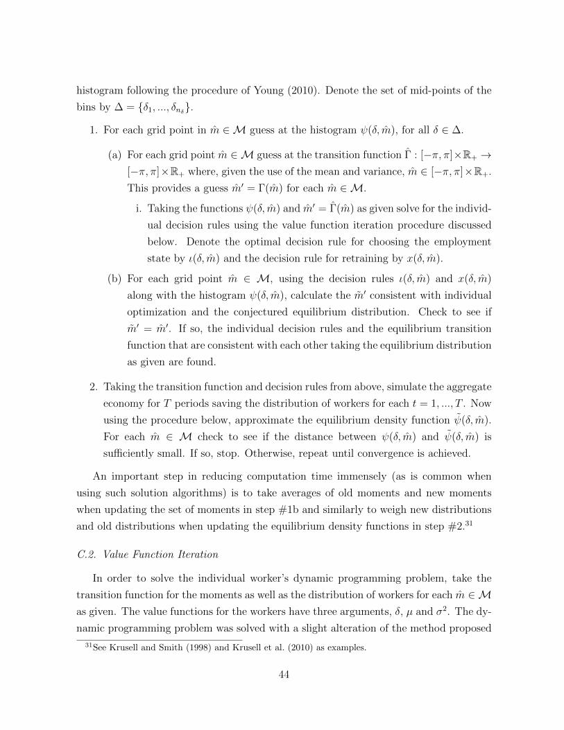
histogram following the procedure of Young (2010). Denote the set of mid-points of the

bins by ∆ = {δ1, ..., δnδ}.

1. For each grid point in m ∈M guess at the histogram ψ(δ, m), for all δ ∈ ∆.

(a) For each grid point m ∈M guess at the transition function Γ : [−π, π]×R+ →[−π, π]×R+ where, given the use of the mean and variance, m ∈ [−π, π]×R+.

This provides a guess m′ = Γ(m) for each m ∈M.

i. Taking the functions ψ(δ, m) and m′ = Γ(m) as given solve for the individ-

ual decision rules using the value function iteration procedure discussed

below. Denote the optimal decision rule for choosing the employment

state by ι(δ, m) and the decision rule for retraining by x(δ, m).

(b) For each grid point m ∈ M, using the decision rules ι(δ, m) and x(δ, m)

along with the histogram ψ(δ, m), calculate the m′ consistent with individual

optimization and the conjectured equilibrium distribution. Check to see if

m′ = m′. If so, the individual decision rules and the equilibrium transition

function that are consistent with each other taking the equilibrium distribution

as given are found.

2. Taking the transition function and decision rules from above, simulate the aggregate

economy for T periods saving the distribution of workers for each t = 1, ..., T . Now

using the procedure below, approximate the equilibrium density function ψ(δ, m).

For each m ∈ M check to see if the distance between ψ(δ, m) and ψ(δ, m) is

sufficiently small. If so, stop. Otherwise, repeat until convergence is achieved.

An important step in reducing computation time immensely (as is common when

using such solution algorithms) is to take averages of old moments and new moments

when updating the set of moments in step #1b and similarly to weigh new distributions

and old distributions when updating the equilibrium density functions in step #2.31

C.2. Value Function Iteration

In order to solve the individual worker’s dynamic programming problem, take the

transition function for the moments as well as the distribution of workers for each m ∈Mas given. The value functions for the workers have three arguments, δ, µ and σ2. The dy-

namic programming problem was solved with a slight alteration of the method proposed

31See Krusell and Smith (1998) and Krusell et al. (2010) as examples.

44

by Barillas and Fernandez-Villaverde (2007). I do not use information on the derivative

of the value functions as is standard in the endogenous grid point method because of

problems that potential kinks in the continuation values of employment, unemployment

or retraining pose along with the discrete choice nature of the worker’s problem. Partic-

ularly, by using derivatives of the continuation value, due to kinks, it is possible that two

occupations, say δ′ = δ+ x and δ′ = δ+ x are optimal continuation occupations from the

same current occupation, δ, even though in equilibrium, one of the occupations may not

be an optimal occupation to move to starting from δ.

Thus, instead of exploiting derivatives, the following procedure which combines some

ideas of traditional value function iteration procedures and some ideas from the EGM

methods was employed. Solve the dynamic programming problem forwards (in con-

trast to backwards as in the EGM) which avoids the problem detailed in the previous

paragraph. Following the EGM method, reduce the number of times that the expected

continuation values is solved per iteration of the value functions to reduce computational

time immensely.

The procedure used to solve the dynamic programming problem is now described.

Define a grid on the continuation occupation G′ ≡ {δ′1, ..., δ′N ′} and a grid for current

occupations G ≡ {δ1, ..., δN}. Construct a large (symmetric) grid for values of x, X ≡{x1, ..., xNx} which contains values between −π and π. The algorithm to iterate on the

value functions is as follows.

1. Start with k = 0 and guess values for V k(δ, µ, σ2) and T k(δ, µ, σ2).

2. Using Gaussian quadratures, for each (δ, µ, σ2), where δ denotes the end of period

occupation for a worker, construct the expected continuation values

W k(δ, µ, σ2) =

∫ ∫max

{T k(δ′, µ′, σ2′)− z′, V k(δ′, µ′, σ2′)

}dF (δ′|δ)dH(z′)

3. Construct a grid G(δ) = {δ + x1, ..., δ + xNx} for each δ and then interpolate the

vector W (δ, µ, σ2) across this grid. This yields the expected continuation value for

each end of the period occupation in the grid G(δ). For each δ ∈ G construct the

functions

V k+1(δ, µ, σ2) = w(δ, µ, σ2) + βW k(δ, µ, σ2)

T k+1(δ, µ, σ2) = maxx∈X

{cb(ψ)− ϕ(x) + βW k(δ + x, µ, σ2)

}.

45

4. If

supi,j,N

∣∣∣∣[ V k+1(δN , µi, σ

2j )− V k(δN , µi, σ

2j )

T k+1(δN , µi, σ2j )− T k(δN , µi, σ2

j )

]∣∣∣∣1 + supi,j,N

∣∣∣∣[ V k(δN , µi, σ2j )

T k(δN , µi, σ2j )

]∣∣∣∣ ≥ crt

then k k + 1 and go to 2. Otherwise, stop and store the value functions,

V (δ, µ, σ2), U(δ, µ, σ2), T (δ, µ, σ2) and the decision rule x(δ, µ, σ2).

For the results shown in the paper, a linear grid for X with 501 points and for G

and a linear grid with 151 points for G′ were used. In the partial equilibrium model,

increasing these grid sizes did not yield significantly different results for the simulation

output.32

C.3. Simulating the Economy

In order to simulate the economy, a method similar to that proposed by Young (2010)

was exploited. Specifically, a histogram over a fixed grid of the occupations was used to

construct moments for the next period. Suppose the interval [−π, π] is broken into NB

equal length bins whose midpoints serve as the “location” of the bin. Once the measure

of workers in each bin is known, it is ease to calculate the moments desired. In simulating

the model for T periods use the procedure that follows.

1. Take the histogram of workers at the beginning of the period t as given.

2. Given this histogram, construct the mean and variance of the distribution. Denote

the period t mean by µt and the variance by σ2t .

3. Use the value functions as obtained from the value function iteration and interpolate

across the moments in M to obtain V (δ, µt, σ2t ), T (δ, µt, σ

2t ) and x(δ, µt, σ

2t ) for all

δ ∈ G.

4. Using these value functions, for each bin, determine the cut-off cost (from the

distribution of idiosyncratic fixed cost of retraining) for which workers would prefer

to retrain rather than be employed.

32In the work presented crt = 1.0e−4. Smaller values such as 1.0e−6 did not lead to drastic differencein observed outcomes but resulted in drastically longer computation times due to the high discountfactor used for the model in which a period represents a month.

46

5. For those who elect to retrain, determine the bin in which their new occupation

falls. Assign all workers who retrain to their new bins.

6. Draw an aggregate shock for period t+ 1. Adjust the bins for all workers given the

end of period t histogram and the period t+ 1 reallocation shock.

7. For each bin, let a fraction 1 − β of the workers withdraw from the labour force.

In each bin add a measure 1−βNB

of new workers.

8. If t = T then stop. Otherwise, t t+ 1 and go to 1.

C.4. The Transition Function for the Moments

In order to determine the transition function for the moments the steps below were

followed. Suppose Nε nodes are used to evaluate the Gaussian quadrature in the distri-

bution for the reallocation shocks, that there are Nµ elements in the grid for the mean

and that there are Nσ2 elements in the grid for the variance.

1. For possible triple (µi, σ2j , εk), i ∈ {1, ..., Nµ}, j ∈ {1, ..., Nσ2}, k ∈ {1, ..., Nε}, con-

jecture the continuation moment pair {µ′ijk, σ2′

ijk}.

2. Using these continuation moments, for each {µ, σ2} ∈ M, construct the continua-

tion values

W (δ, µ, σ2) =

∫ ∫max

{T (δ′, µ′, σ2′)− z′, V (δ′, µ′, σ2′)

}dF (δ′|δ)dH(z′)

and then construct the functions

V (δ, µ, σ2) = w(δ, µ, σ2) + βW (δ, µ, σ2)

T (δ, µ, σ2) = maxx∈X

{cb(ψ)− ϕ(x) + βW (δ + x, µ, σ2)

}.

3. For each {µ, σ2} ∈ M, simulate the economy for one period and find the realized

moment pairs {µ′ijk, σ2′

ijk}. Note that this is a realized pair meaning one pair for

each possible shock ε′ ∈ {ε1, ..., εNε}.

4. For some set of weights {ωi,j,k}, if

sup

∣∣∣∣ωi,j,k [ µijk − µ′ijkσ2′

ijk − σ2′

ijk

]∣∣∣∣1 + sup

∣∣∣∣ωi,j,k [ µijk − µ′ijkσ2′

ijk − σ2′

ijk

]∣∣∣∣

≥ 1.0e−3

47

then set [µ′ijk, σ2′

ijk] = λ[µ′ijk, σ2′

ijk] + (1− λ)[µ′ijk, σ2′

ijk], where λ ∈ [0, 1) and go to 2.

Otherwise, stop.

In this process a set of weights {ωi,j,k} was introduced to reduce the computation

time. Effectively, the weights may be chosen to down-weight the importance of nodes

that are unlikely to be reached in equilibrium, for example, for mean and variances that

are at the extremes of their respective grids or for reallocation shocks that are of very

low probability of being drawn. This is useful as the grid upon which the value function

iteration is solved must be large enough to capture the equiibrium dynamics of the mean

and variance (which are not known at the time the model is solved). As such this grid

must be include some large and small values for the moments. However, in simulations,

it is likely that the economy never ventures near these nodes. By down-weighting their

importance in the solution method, their impact on solution time is minimized.

C.5. The Equilibrium Distribution

In order to characterize the equilibrium distribution necessary to determine the equi-

librium wages at each triplet (δ, µ, σ2) for each δ ∈ G, µ ∈ M1 and σ2 ∈ M2, the

procedure set forth by Reiter (2002) and Reiter (2010) was followed closely. This proce-

dures are repeated here. First, construct what is referred to as a “reference distribution”

for each {µ, σ2} ∈ M1 ×M2.

1. Initialize the reference distribution ψR(δ, µ, σ2) either by a uniform distribution or

by some other means.33

2. Starting with this reference distribution, simulate the economy for TBurn + T peri-

ods and then discard the statistics from the first TBurn “burn-in” periods. In the

results shown, I used TBurn = 1000 and T = 25000. Store the mean, variance and

histogram from each of these T periods. Let ψsim,t denote the simulated histogram

from period t = 1, ..., T (it is a vector). Let µsim,t and σ2sim,t be the corresponding

mean and variance from period t of the stored simulation data.

33In the computations, the partial equilibrium model was simulated in order to obtain some realizationsfor equilibrium distribution given a set of parameters. Then the general equilibrium model was resolvedmany times while reducing the elasticity parameter χ and adjusting a few other parameters governingmobility costs each time. This was the most time consuming process in calibrating the model.

48

3. Update the ψR(δ, µ, σ2) by the weighted sum

ψR(δ, µ, σ2) ≡T∑t=1

γtψsim,t

γt ≡d([µ, σ2], [µsim,t, σ

2sim,t])

ν∑Tt=1 d([µ, σ2], [µsim,t, σ2

sim,t])ν

where, in our application, d(·) was the Euclidean metric and the weight ν was

chosen to be −4.34

Given the reference distributions, ψR(δ, µ, σ2) for each pair (µ, σ2) ∈ M1 × M2,

construct the “proxy distribution”. Importantly, note that the mean and variance of the

reference distributions are not equal to µ and σ2, respectively. In order to adjust each

of these reference distributions the following steps were used. For each (µi, σ2j ) pair, for

i = 1, ..., Nµ, j = 1, ..., Nσ2 , calculate the mean and variance of the reference distribution

ψ(δ, µi, σ2j ). Denote this reference pair as (µR,i, σ

2R,j).

As histograms were used to approximate the continuous distribution, use the notation

ψl to denote the lth bin in the histogram with l = 1, ..., Nδ. The constrained optimization

problem below was solved for each (µ, σ2) ∈M.

min{ψl}

Nδl=1

Nδ∑l=1

(ψl − ψRl )2

subject to the constraints ψl ≥ 1−βNδ

and

δ1 δ2 ... δNδδ2

1 δ22 ... δ2

Nδ

1 1 ... 1

ψ1

ψ2...

ψNδ

=

µσ2 + µ2

1

.This results in a set of proxy distributions ψ(δ, µ, σ2) which were used as approximations

of the equilibrium distributions.

C.5.1. Updating the Proxy Distributions

In order to update the proxy distributions the simulated data, {µsim,t, σ2sim,t}Tt=1, that

was used to construct the new proxy distributions were obtained. Then data stored from

34Other values of ν were checked to see if the equilibrium changed much.

49

the simulation used in the previous proxy distribution updating iteration was recalled,

{µsim,t, σ2sim,t}Tt=1. In other words, simulation data constructed by using the previous

iteration’s moments and distributions were compared to simulation data constructed

using the current iteration’s moments and distributions. Comparing the time-series for

each moment, denote

resµ =|µsim,t − µsim,t|

1 + |µsim,t|, resσ =

∣∣∣σ2sim,t − σ2

sim,t

∣∣∣1 +

∣∣∣σ2sim,t

∣∣∣where resµ and resσ are both T × 1 vectors (T = 25000 in this particular application).

Finally, vertically stacking resµ and resσ construct res = mean([resµ; resµ]). If res ≥1.0e−2 then update the proxy distributions by taking the weighted average,

ψ(δ, µ, σ2)′ = λψψ(δ, µ, σ2) + (1− λψ)ψ(δ, µ, σ2)

where λψ ∈ (0, 1), ψ(δ, µ, σ2) is the newly constructed set of proxy distributions and

ψ(δ, µ, σ2) is the previous iteration’s value for the proxy distributions. Otherwise, stop.

This method of constructing a stopping criterion for the solution method was useful as

it tested whether changes in the distribution resulted in any substantial changes to the

moments that individuals were using to approximate the distribution of workers across

occupations when constructing their individual decision rules.

C.5.2. Additional Details

Given that the Beta distribution was employed to model the distribution of shocks,

and conditional on the fitted value for the standard deviation of the shocks, it turned

out that quadrature methods to approximate integrals were not very accurate. Instead,

a histogram was employed to approximate integrals relating to continuation values in the

value function iteration procedure. This histogram was constructed by first locating a

value in the domain of the Beta p.d.f. at the density first exceeds 1e−4. As the Beta

distribution employed was symmetric, this pinned down outer bounds for the histogram

to be used. A linear grid of 30 nodes was created within these bounds. These nodes were

located at the center of the 30 histogram bins and the value of the p.d.f. at these nodes

served as the probabilities that were then used to construct expectations in the value

function iteration procedure.

50

REFERENCES

Acemoglu, D. and D. Autor (2010): “Skills, Tasks and Technologies: Implications

for Employment and Earnings,” in Handbook of Labor Economics, ed. by O. Ashenfelter

and D. E. Card, Amsterdam: Elsevier, vol. 4.

Alvarez, F. and R. Shimer (2009): “Search and Rest Unemployment,” Econometrica,

79(1), 75–122.

Autor, D. and D. Dorn (2013): “The Growth of Low Service Skill Jobs and the

Polarization of the U.S. Labor Market,” American Economic Review, 103(5), 1553–

1597.

Autor, D., L. Katz, and M. Kearney (2008): “Trends in U.S. Wage Inequality:

Revising the Revisionists,” Review of Economics and Statistics, 90(2), 300–323.

Autor, D., F. Levy, and R. Murnane (2003): “The Skill Content of Recent Techno-

logical Change: An Empirical Exploration,” Quarterly Journal of Economics, 116(4),

1279–1333.

Barillas, F. and J. Fernandez-Villaverde (2007): “A generalizeation of the en-

dogenous grid method,” Journal of Economic Dynamics and Control, 31, 2698–2712.

Carrillo-Tudela, C. and L. Visschers (2015): “Unemployment and Endogenous

Reallocation over the Business Cycle,” Mimeo.

Cortes, G. M. (2016): “Where Have the Middle-Wage Workers Gone? A Study of

Polarization Using Panel Data,” Journal of Labor Economics, 34(1), 63–105.

Cortes, G. M. and G. Gallipoli (2017): “The Costs of Occupational Mobility: An

Aggregate Analysis,” Journal of the European Economic Association, Forthcoming.

Dorn, D. (2009): “Essays on Inequality, Spatial Interaction, and the Demand for Skills,”

Dissertation University of St. Gallen no. 3613.

Garin, J., M. Pries, and E. Sims (2017): “Reallocation and the Changing Nature of

Economic Fluctuations,” American Economic Journal: Macroeconomics, Forthcoming.

Gathmann, C. and U. Schonberg (2010): “How General is Human Capital? A

Task-Based Approach,” Journal of Labor Economics, 28(1), 1–49.

51

Gautier, P. A., C. N. Tuelings, and A. V. Vuuren (2010): “On-the-Job Search,

Mismatch and Efficiency,” Review of Economic Studies, 77, 245–272.

Gonzalez, F. and S. Shi (2010): “An Equilibrium Theory of Learning, Search and

Wages,” Econometrica, 78(2), 509–537.

Gouge, R. and I. King (1997): “A Competitive Theory of Employment Dynamics,”

Review of Economic Studies, 64(1), 1–22.

Jaimovich, N. and H. Siu (2012): “The Trend is the Cycle: Job Polarization and

Jobless Recoveries,” Working paper.

Kambourov, G. and I. Manovskii (2009): “Occupational Mobility and Wage In-

equality,” Review of Economic Studies, 76, 731–759.

Krusell, P., T. Mukoyama, and A. Sahin (2010): “Labour-Market Matching with

Precautionary Savings and Aggregate Fluctuations,” The Review of Economic Studies,

77(4), 1477–1507.

Krusell, P. and A. Smith (1998): “Income and Wealth Heterogeneity in the Macroe-

conomy,” Journal of Political Economy, 106(5), 867–896.

Lucas, R. E. and E. C. Prescott (1974): “Equilibrium Search and Unemployment,”

Journal of Economic Theory, 7, 188–209.

Marimon, R. and F. Zilibotti (1999): “Unemployment vs. Mismatch of Talent:

Reconsidering Unemployment Benefits,” The Economic Journal, 109, 266–291.

Menzio, G. and S. Shi (2010): “Block recursive equilibria for stochastic models of

search on the job,” Journal of Economic Theory, 145, 1453–1494.

Moen, E. (1997): “Competitive Search Equilibrium,” Journal of Political Economy,

105(2), 385–411.

Pilossoph, L. (2014): “Sectoral Shocks and Move Unemployment,” Working paper.

Pissarides, C. A. (2001): Equilibrium Unemployment Theory, Cambridge, MA : MIT

Press, 2nd ed.

52

Poletaev, M. and C. Robinson (2008): “Human Capital Specificity : Evidence

from the Dictionary of Occupational Titles and Displaced Worker Surveys, 1984-2000,”

Journal of Labor Economics, 26(3), 387–420.

Reiter, M. (2002): “Recursive computation of heterogeneous agent models,” Mimeo.

——— (2010): “Solving the incomplete markets model with aggregate uncertainty by

backward induction,” Journal of Economic Dynamics and Control, 34, 28–35.

Robinson, C. (2010): “Occupational Mobility, Occupational Distance and Basic Skills

: Evidence from Job-Based Skill Measures,” Mimeo.

Shi, S. (2009): “Directed Search for Equilibrium Wage-Tenure Contracts,” Economet-

rica, 77(2), 561–584.

Veracierto, M. (2008): “On the cyclical behavior of employment, unemployment and

labor force participation,” Journal of Monetary Economics, 55, 1143–1157.

Wiczer, D. (2015): “Long-Term Unemployment: Attached and Mismatched,” Working

paper, Federal Reserve Bank of St. Louis.

Young, E. (2010): “Solving the incomplete markets model with aggregate uncertainty

using the Krusell-Smith algorithm and non-stochastic simulations,” Journal of Eco-

nomic Dynamic and Control, 34, 36–41.

53