Embed Size (px)
Citation preview

School Funding, Taxes, and Economic Growth
An Analysis of the 50 States
NEA RESEARCHWORKING PAPER
April 2004

NEA RESEARCHWORKING PAPER
April 2004
School Funding, Taxes, and Economic GrowthAn Analysis of the 50 States
Richard G. SimsIndependent Consultant

The National Education Association is the nation’s largest professional employee
organization, representing 2.7 million elementary and secondary teachers, high-
er education faculty, education support professionals, school administrators,
retired educators, and students preparing to become teachers.
Complimentary copies of this publication are available in limited numbers from
NEA Research for NEA state and local associations, and UniServ staff. Call
202-822-7400. Additional copies may be purchased from the NEA Professional
Library, Distribution Center, P.O. Box 2035, Annapolis Junction, MD 20701-
2035. Telephone 800-229-4200 for price information. This publication may also
be downloaded from www.nea.org.
Reproduction: No part of this report may be reproduced in any form without
permission from NEA Research, except by NEA-affiliated associations or NEA
members. Any reproduction of the report materials must include the usual cred-
it line and copyright notice. Address communications to Editor, NEA Research,
1201 16th St., N.W., Washington D.C. 20036-3290.
Appendix B contains descriptions of an econometric model developed by
Regional Economic Models, Inc. (REMI), and draws on language and graphics
from the REMI Web site (www.remi.com/). These materials are adapted with the
permission of REMI, 306 Lincoln Avenue, Amherst, MA 01002.
Published April 2004
Copyright © 2004 by the
National Education Association
All Rights Reserved

Executive Summary . . . . . . . . . . . . . . . . . . . . . . . . . . . . . . . . . . . . . . . . . . . . . . . . . . . . . . . . . . . . . . . . . . . . . . . . . . . . . . . . . . . . . . . . . 1
School Funding, Taxes, and Economic Growth: An Analysis of the 50 States . . . . . . . . . . . . . . . . . . . . . . . . . . . . . . . . . . . . . . 3
Spending on Education: Schools, Teachers, and the Ripple Effect . . . . . . . . . . . . . . . . . . . . . . . . . . . . . . . . . . . . . . . . . . . 4
Role of Education Spending in Enhancing Regional Economic Competitiveness . . . . . . . . . . . . . . . . . . . . . . . . . . . . . . 6
Taxes: Paying the Piper . . . . . . . . . . . . . . . . . . . . . . . . . . . . . . . . . . . . . . . . . . . . . . . . . . . . . . . . . . . . . . . . . . . . . . . . . . . . . . 7
Taxing and Spending: The Delicate Balance . . . . . . . . . . . . . . . . . . . . . . . . . . . . . . . . . . . . . . . . . . . . . . . . . . . . . . . . . . . . 11
Conclusions . . . . . . . . . . . . . . . . . . . . . . . . . . . . . . . . . . . . . . . . . . . . . . . . . . . . . . . . . . . . . . . . . . . . . . . . . . . . . . . . . . . . . . 12
Appendix A: Education Expenditures of State and Local Governments, by State . . . . . . . . . . . . . . . . . . . . . . . . . . . . . . . . . 13
Appendix B: The Economic Model . . . . . . . . . . . . . . . . . . . . . . . . . . . . . . . . . . . . . . . . . . . . . . . . . . . . . . . . . . . . . . . . . . . . . . . . . . . 15
Model Structure . . . . . . . . . . . . . . . . . . . . . . . . . . . . . . . . . . . . . . . . . . . . . . . . . . . . . . . . . . . . . . . . . . . . . . . . . . . . . . . . . . . 16
Model Application . . . . . . . . . . . . . . . . . . . . . . . . . . . . . . . . . . . . . . . . . . . . . . . . . . . . . . . . . . . . . . . . . . . . . . . . . . . . . . . . . 17
Articles on Regional Econometric Models and the REMI Model . . . . . . . . . . . . . . . . . . . . . . . . . . . . . . . . . . . . . . . . . . . 18
Articles Describing Regional Econometric Models Generally . . . . . . . . . . . . . . . . . . . . . . . . . . . . . . . . . . . . . . . . . . . 18
Descriptions of the REMI Model . . . . . . . . . . . . . . . . . . . . . . . . . . . . . . . . . . . . . . . . . . . . . . . . . . . . . . . . . . . . . . . . . . 19
Articles Evaluating REMI and Similar Econometric Models . . . . . . . . . . . . . . . . . . . . . . . . . . . . . . . . . . . . . . . . . . . . 19
Articles Describing Uses of REMI . . . . . . . . . . . . . . . . . . . . . . . . . . . . . . . . . . . . . . . . . . . . . . . . . . . . . . . . . . . . . . . . . . 20
Appendix C: Detailed Results of 50-State Analyses . . . . . . . . . . . . . . . . . . . . . . . . . . . . . . . . . . . . . . . . . . . . . . . . . . . . . . . . . . . . 21
References . . . . . . . . . . . . . . . . . . . . . . . . . . . . . . . . . . . . . . . . . . . . . . . . . . . . . . . . . . . . . . . . . . . . . . . . . . . . . . . . . . . . . . . . . . . . . . . . 27
Tables
TABLE 1 Direct Primary and Secondary Employment Effects of a 2 Percent Increase in Education Spending
(Change in Number of Jobs, in Thousands) . . . . . . . . . . . . . . . . . . . . . . . . . . . . . . . . . . . . . . . . . . . . . . . . . . . . . . . . . . 5
TABLE 2 Indirect Employment Effects from a 2 Percent Increase in Education Spending:
Amenity and Competitiveness Aspects Direct Effects Added to (Change in Number of Jobs, in Thousands) . . . . . 8
TABLE 3 Employment Effects of an Increase in Consumption Tax Equivalent to 2 Percent of Education Spending
(Change in Number of Jobs, in Thousands) . . . . . . . . . . . . . . . . . . . . . . . . . . . . . . . . . . . . . . . . . . . . . . . . . . . . . . . . . 10
TABLE 4 Net Effects of 2 Percent Education Funding and Matching Tax Increase with
Educational Competitiveness Factors Considered (Change in Number of Jobs, in Thousands) . . . . . . . . . . . . . . . 11
TABLE A1 Direct General Expenditures of State and Local Governments for
Elementary and Secondary Education, by State ($ millions) . . . . . . . . . . . . . . . . . . . . . . . . . . . . . . . . . . . . . . . . . . . . 13
TABLE C1 Detailed Results of 50-State Analyses . . . . . . . . . . . . . . . . . . . . . . . . . . . . . . . . . . . . . . . . . . . . . . . . . . . . . . . . . . . . 21
Contents
iii

Figures
FIGURE B1 Underlying Structure of the REMI Model . . . . . . . . . . . . . . . . . . . . . . . . . . . . . . . . . . . . . . . . . . . . . . . . . . . . . . . . 17
FIGURE B2 Use of the REMI Model for Analysis of Policy Effects: A Two-Step Process . . . . . . . . . . . . . . . . . . . . . . . . . . . . 18
FIGURE B3 Introduction of Policy Variables into the REMI Model . . . . . . . . . . . . . . . . . . . . . . . . . . . . . . . . . . . . . . . . . . . . . 19
Boxes
BOX 1 Literature on the Effects of State and Local Education Spending on Economic Growth . . . . . . . . . . . . . . . . . . . . . . 6
BOX 2 Kentucky: Economic Losses Associated with Raising Revenue from Various Tax Sources
(Total new revenue = $68.8 million) . . . . . . . . . . . . . . . . . . . . . . . . . . . . . . . . . . . . . . . . . . . . . . . . . . . . . . . . . . . . . . . . . 9

Executive Summary
Recent court decisions and state studies indicate
that none of the states measure up on even rough
measures of adequacy and equity in school fund-
ing. Because of tax and spending limits, some states have
school funding systems that are equitable, but hardly ade-
quate. One way to address this problem is for states to get
on a path toward achieving adequacy and equity by
increasing education spending by a small percentage each
year. However, given the compelling need to balance state
budgets, governors and legislators frequently confront the
difficult choice of cutting spending or raising taxes. A
major aspect of this knotty fiscal dilemma is the effect
such a fiscal policy decision will have on employment lev-
els in the state.
This study employs a set of state-specific dynamic com-
putable general equilibrium (CGE) models to evaluate the
employment effects of a fiscal policy decision relating to
education-related taxing and spending. Specifically, the
study looks at the consequences of an increase in educa-
tion spending by 2 percent and an equal increase in state
residents’ consumer taxes. The analysis considers the
development impacts of education as an economic
“industry,” employing resources and producing an output.
It also considers effects that are unique to educational
spending, such as its role in regional amenity enhance-
ment (i.e., the value that the increased quality of life from
better-supported schools has in attracting a productive
and efficient workforce).
The study finds that the number of jobs created by
increasing education spending is larger than the number
of jobs lost from increasing taxes to support that spend-
ing. The study reveals that such a strategy has significant
net positive near- and long-term employment effects for
each of the 50 states.
1

What makes America great are the values we all
believe in—democracy, equal opportunity, and
fairness—the values that public education
helps us preserve. As parents, we want excellent schools for
our own children so that they can succeed in life. As mem-
bers of a community, we want a high-quality school system
so that we can attract and develop new businesses. As citi-
zens, we want our nation to have a world-class educational
system that enables our children to compete with the best
that other nations have to offer.
School funding typically tops the list of concerns of state
policymakers and of the electorate. Support for education is
widespread and transcends political, social, and economic
lines. (Brunori 2000, for example, noted that of five major
tax bills recently introduced to support education funding,
Republicans introduced four.) Yet, however popular it may
be, education funding is typically neither adequate nor
equitable. In almost all of the recent school finance cases,
courts have ruled in favor of plaintiffs, declaring state fund-
ing systems unconstitutional. An analysis of more than a
dozen states conducted by the National Education
Association shows that none of the states measure up to
even a rough measure of adequacy and equity.
In-depth studies using methods such as the professional
judgment method and the successful schools method also
show a significant gap between current levels of funding
and those necessary to achieve adequacy and equity (see
Ladd et al. 1999).
Adequacy and equity in school funding are necessary to
implement the programs and practices that work. But it
would be difficult to achieve adequacy and equity
overnight. Therefore, we assume in this study that each state
would take an incremental approach to the problem,
increasing education spending by an additional 2 percent
per year of current expenditures over 10 years. (See
Appendix A for by-state totals derived from NCES 2000.)
We believe that such an approach not only would move
states closer to achieving adequacy and equity but also
would have a positive impact on state economies.
Weighing against our desire to achieve adequate and
equitable funding is the reality that increased spending
comes at a cost—in particular, a cost in the form of taxes.
Higher taxes reduce the amount of money consumers have
to spend on other items, thereby reducing retail sales, cut-
ting business profits, lowering the demand for intermediate
goods and services, and lowering the level of employment.
Both spending for education and taxing to fund that
spending have significant effects on states’ economies. The
positive economic effects of education spending start with
direct spending for the education budget. Examples include
compensation for teachers, administrators, and other edu-
cation related personnel; payments for transportation,
school safety, environment and facility maintenance; and
purchases of school supplies, materials, equipment, and
business services. These direct spending effects in turn pro-
duce indirect effects. For example, the wages of school
employees support consumer spending in the community;
expansions of school buildings employ local construction
and maintenance services; and school purchases ring up as
sales for local businesses.
The negative economic impact of taxes start by taking
money out of the hands of individuals, reducing household
School Funding, Taxes, and Economic Growth:An Analysis of the 50 States
3

4 School Funding, Taxes, and Economic Growth:
purchasing power, and lowering the demand for local busi-
nesses’ goods and services. Faced with reduced sales and
falling profits, those local businesses reduce their own pur-
chases and payrolls, and that in turn leads to further reduc-
tions in spending in the community at large. The net eco-
nomic consequences that arise from these opposing ten-
sions between additional education spending and addition-
al taxes (when both occur in balanced budgetary environ-
ment) are the subject of this study.
Many studies have looked at the issue of taxes, spending,
and state economic growth. Typically, these studies begin
with broad aggregate levels of public finance—such as total
state and local revenues as a percentage of state personal
income, or state and local education spending per stu-
dent—and compare them with broad measures of state
economic growth, such as increase in per capita personal
income. These studies frequently address issues such as a
state’s tax competitiveness and the effects of improved
workforce quality and productivity on regional growth (see
Bartik 1992; Garcia-Mila and McGuire 1992; Helms 1985;
and Wasylenko 1997).
This study borrows heavily from the economic literature
but differs from most previous works in that it uses a set of
state economic simulation models incorporating detailed
data on each individual state to explore a specific fiscal poli-
cy measure and applies that measure to each of the 50 states
to observe the outcomes. The specific policy change
addressed herein is an increase in public school funding by 2
percent each year, fully funded by a broad-based sales tax. A
relatively small change is politically more realistic, and
changes at the margin largely avoid issues of structural shifts
that might be brought about by large initial changes. Use of
a simulation model allows an observer to isolate the effects
of the various aspects of a policy measure, separating out the
effects of taxes on their own and of the spending on its own.
The present study estimates the combined direct and
indirect effects on a state’s employment and the general
economy of the new education spending and the related
taxing by using a set of econometric models designed to
depict each state’s individual economy. Each state model
contains extensive data on the state economy that include
the linkages between taxes and the economy, between
industries, between regions, between changing demograph-
ics and the economy, and between the state and the nation-
al economy. In particular, the models look at current and
historical linkages between education spending and the
economy based largely on U.S. Census, Bureau of Labor
Statistics, and other official primary data. The long-term
impacts take into consideration expected trends in the U.S.
economy, including changes in the composition of indus-
tries, in supply and demand for the various inputs, in capi-
tal and labor productivity, and in regional demographics.
To avoid distracting from the main points of this study, the
study presents the details and technical features of the
model separately (see Appendix B).
The study starts by focusing on the employment aspects
of school funding and school-related taxation. Concen-
trating on one economic variable, such as jobs, should allow
presentation of the steps in analyzing the education funding
process in a relatively clear and uncluttered manner. After
explaining and analyzing the various steps in the economic
sequence for their employment impacts, the study then
expands the findings to include the broader economic
measure of personal income (see Appendix C).
Spending on Education: Schools, Teachers, and the Ripple Effect
Direct budgetary spending for K-12 education involves the
employment of teachers, school administrators, and class-
room aids and of clerical, maintenance, security, and other
personnel whose jobs and income come directly from the
education system. This analysis starts with the consideration
of the job effects of increasing public K–12 education spend-
ing by 2 percent of the current amount and maintaining that
increase in real, constant-dollar, terms in future years. We
assume that this added educational spending is allocated on
items and in proportions similar to those of current spend-
ing. Current expenditures are from NCES (2000).
Money that starts as spending for educational activities
soon becomes the income for households and for business-
es in the community. Additional wages paid to school per-
sonnel become part of their household income and are used
to purchase houses, automobiles, groceries, and theater
tickets and for other forms of consumer spending, thereby
stimulating the local economy. In addition, the budgetary
activities of operating a school system have a direct bearing
on the revenues and employment of the firms and non-
school-employed individuals who supply the education sys-
tem with goods and services. Regional building contractors,
food vendors, office suppliers, and other school service
providers derive part of their earnings from the direct
spending by educational institutions. These secondary
effects are sometimes referred to as the ripple effects of the
initial spending.
This simulation begins by entering a 2 percent increase
into each state’s simulation model. Again, the additional

Spending on Education 5
spending is allocated in the model in proportion to existing
spending patterns. Table 1 shows that the direct and indi-
rect effects of a 2 percent incremental increase in education
spending on employment are positive for all 50 states. We
expect this, of course, because we have not yet accounted for
the cost of the spending.
The increase in employment, although remaining posi-
tive for all states, diminishes over time and thus is somewhat
lower in real terms in 2014 than it was in 2004. This gradual
decline is caused in part by wage increases and in part by
productivity improvements. That is, an increase in educa-
tion spending, creating an added demand for educational
labor, will drive wages up slightly for that group, because the
offer of higher wages will be needed to attract new teachers,
for example, into the region. This in turn means that a given
amount of spending will support slightly fewer jobs after
the wage adjustment. In addition, producers of goods and
services typically become more efficient over time, thus
requiring progressively fewer workers to meet the added
demand brought on by the new spending.
This summary does not present detailed state results for
particular occupations affected by a spending increase. The
employment results also vary considerably from state to
state. In general, however, about one-third of the added jobs
are classroom personnel (primarily teachers, librarians, and
counselors); one-third other school personnel (administra-
tors, clerical, and support); and one-third non-school-relat-
ed workers. The added nonschool employment is largely in
retail trade but may also include construction, finance,
insurance, and real estate.
Alabama 3.2 2.5
Alaska 1.0 0.9
Arkansas 1.2 1.5
Arizona 2.9 2.2
California 24.2 16.0
Colorado 3.4 2.3
Connecticut 2.0 1.5
Delaware 0.3 0.2
Washington, DC 0.3 0.3
Florida 10.2 8.4
Georgia 5.5 4.2
Hawaii 0.5 0.4
Idaho 1.1 0.9
Illinois 7.8 5.7
Indiana 4.8 3.6
Iowa 2.7 2.2
Kansas 3.3 2.7
Kentucky 3.9 3.1
Louisiana 3.0 2.5
Maine 0.9 0.8
Maryland 3.4 2.7
Massachusetts 3.5 2.6
Michigan 8.8 6.2
Minnesota 4.8 3.3
Mississippi 1.8 1.5
Missouri 3.8 3.1
TABLE 1 Direct Primary and Secondary Employment Effects of a 2 Percent Increase in Education Spending
(Change in Number of Jobs, in Thousands)
State 2004 2014
Montana 1.1 0.9
Nebraska 1.6 1.3
Nevada 1.0 0.6
New Hampshire 0.8 0.6
New Jersey 6.5 4.7
New Mexico 1.5 1.3
New York 14.2 10.9
North Carolina 4.6 3.8
North Dakota 0.6 0.5
Ohio 9.8 7.0
Oklahoma 2.7 2.2
Oregon 3.6 2.6
Pennsylvania 7.6 6.0
Rhode Island 0.6 0.5
South Carolina 3.2 2.5
South Dakota 0.6 0.5
Tennessee 3.1 2.4
Texas 17.5 12.5
Utah 2.1 1.6
Vermont 0.6 0.6
Virginia 4.8 3.6
Washington 5.6 4.3
West Virginia 1.9 1.7
Wisconsin 4.8 3.7
Wyoming 0.7 0.5
State 2004 2014

6 School Funding, Taxes, and Economic Growth:
Role of Education Spending inEnhancing Regional EconomicCompetitiveness
Among all of the budgetary options facing state or govern-
ments, education stands out as one to which voters consis-
tently favor devoting more resources and personnel. The
local education system also factors into businesses’ location
decisions (see, e.g., Jacobson 2002). Public and business
support for education is generally not based on the number
of education jobs the spending creates but on the idea that
perceptions of the community are improved because of its
expanded educational effort and on expectations that stu-
dents in the area will have greater future earning power. In
economic terms, the increased education spending embod-
ies two compelling features: first, the increased economic
competitiveness and general desirability of areas where
schools improve; and, second, the increased productivity
that added educational support instills in future workers.
The competitiveness aspect of education spending is
predicated on the fact that people and businesses prefer to
locate in areas with comparatively better schools. Increased
education spending makes a community a more desirable
place to live and work, and thus more people move there.
An increase in the region’s attractiveness also means that
workers will be more willing to accept employment in the
Box 1 Literature on the Effects of State andLocal Education Spending on Economic Growth
Numerous researchers have addressed the concept ofthe effects of state and local education spending oneconomic growth. Among them, Helms (1985) foundthat increases in state and local taxes used to increasepublic spending in health, highways, schools, or high-er education caused growth in state personal income.Bartik (1989) observed that increases in state and localtaxes increased the rate of small business creation ifadditional tax revenues were spent on local school andfire protection. Garcia-Mila and McGuire (1992) con-sidered data over a 14-year period from the 48 con-tiguous states to estimate elasticity coefficients forpublicly provided highways and education. Theyfound that both highways and education are produc-tive inputs to state economic growth and that educa-tion has the stronger impact.
Bogart and Cromwell (1997) analyzed threeCleveland neighborhoods, part in one school districtand part in another, where one district clearly had abetter reputation than the other. After controlling forhousing size and quality, the authors found differ-ences attributable to perceived school quality of$5,600 in the first neighborhood, $10,900 in the sec-ond, and $12,000 in the third, using 1987 dollars. In2001-dollar terms, these differences would be $8,680,$16,895, and $18,600, respectively (inflation changescalculated by this author). These positive differencesoccur even though school taxes were higher in thehigh-reputation district. Dee (2000) consideredwhether new school districts’ resources were capital-ized into the housing values and residential rents with-in those districts. Dee’s estimates, based on district-level census data, indicate that new educationalexpenditures generated by court mandates substan-tially increased median housing values and residential
rents. His findings imply that court-mandated financereforms increased the perceived quality of the poorerschool districts in reform states.
Brasington (1999) used both traditional hedonichouse price estimation and a hedonic corrected forspatial autocorrelation to estimate the school quali-ty/housing value relationship. Proficiency tests, expen-diture per student and the student–teacher ratio areconsistently capitalized into housing prices. Teachersalary and student attendance rates are also valued,but these results are sensitive to the estimation tech-nique employed. Value-added measures, graduationrate, teacher experience levels, and teacher educationlevels are not consistently positively related to housingprices.
Finally, Weimer and Wolkoff (2003), in a study ofdistricts in New York State, found “substantively largeeffects of elementary school output on housing val-ues.” The researchers identified school quality indica-tors including average ELA scores, ratio of students toteachers, Regents’ diploma graduation rate, percent-age greater that 65% on Regents‘ English exam,school tax rate, and effective tax rate and found thatschool spending tends to be capitalized into housingvalues in a community.
For additional articles discussing the link betweenschools, economic growth, the labor force, and hous-ing values see Barro (2001); Betts (1995); Black (1999);Brasington (1999); Card and Krueger (1996); Crone(1998); Downes and Zabel (2002); Figlio and Lucas(2000); Fisher (1997); Goldin and Katz (2001); Gradsteinand Justman (2002); Haurin and Brasington (1996);Hayes and Taylor (1996); Hanushek and Kimko (2000);Kane, Staiger, and Samms (2003); Kodrzycki (2002);McGuire (2003); Nechyba (2003); and Yitzhaki (2003).

Taxes 7
area at relatively lower wages than before or than they might
get elsewhere. The expanded labor force in the area makes it
easier and less expensive for employers to find qualified
workers and holds down regional employment costs for
employers. The increase in the potential workforce thus
boosts the long-term productivity and competitiveness of
the region. The quality-of-life factors in a region’s “attrac-
tiveness,” its amenity value, influence a region’s competitive-
ness and growth potential.
The effects of in-migration related to education spend-
ing can be seen in housing values and wages. In-migration
increases the demand for housing and raises housing values
in communities of increasing school spending (Weimer and
Wolkoff 2003; Bogart and Cromwell 1997, 2000; Dee 2000).
Studies have shown that even people without children pre-
fer to live and own property in areas where schools are con-
sidered to be of high quality or at least improving (Hilber
and Mayer 2002).
The fact that people are willing to pay more for housing
or accept lower wages to live in areas with better schools is
consistent with everyday observation. People routinely
accept lower wages and pay higher housing prices to be near
amenities such as beaches, mountains, and golf courses, as
well as communities with wide choices for shopping, recre-
ation, and leisure activities or other factors they view as
contributing to their quality of life (see, e.g., Jensen and
Leven 1997; Kahn 1995; Kotkin and DeVol 2001; Florida
2002).
Similarly, the idea that people will accept higher taxes to
support the amenity of better-quality education is consis-
tent with a straightforward line of reasoning. (This is often
called willingness to pay.) Because education tax decisions
are generally made democratically (i.e., voters choose to
increase their own taxes either by direct vote or through the
vote of a representative), it is reasonable to assume that
individuals believe the added educational improvements
are worth at least what they are paying for them in added
taxation. Individuals might consider the educational
improvements as worth more than what they pay (i.e., they
got a “bargain,” or, in economists’ terms, they received a
consumer surplus). It is unlikely, however, that, as a group,
taxpayers would consider those improvements as worth less
than what they willingly pay for them. The idea that a loca-
tion’s appeal is influenced by the combination of school
spending and taxes is reinforced by empirical observations
that households do migrate (i.e., “vote with their feet”) fol-
lowing school funding increases (Margulis 2001).
Box 1 provides a brief review of the literature on the eco-
nomic effects of state and local education spending.
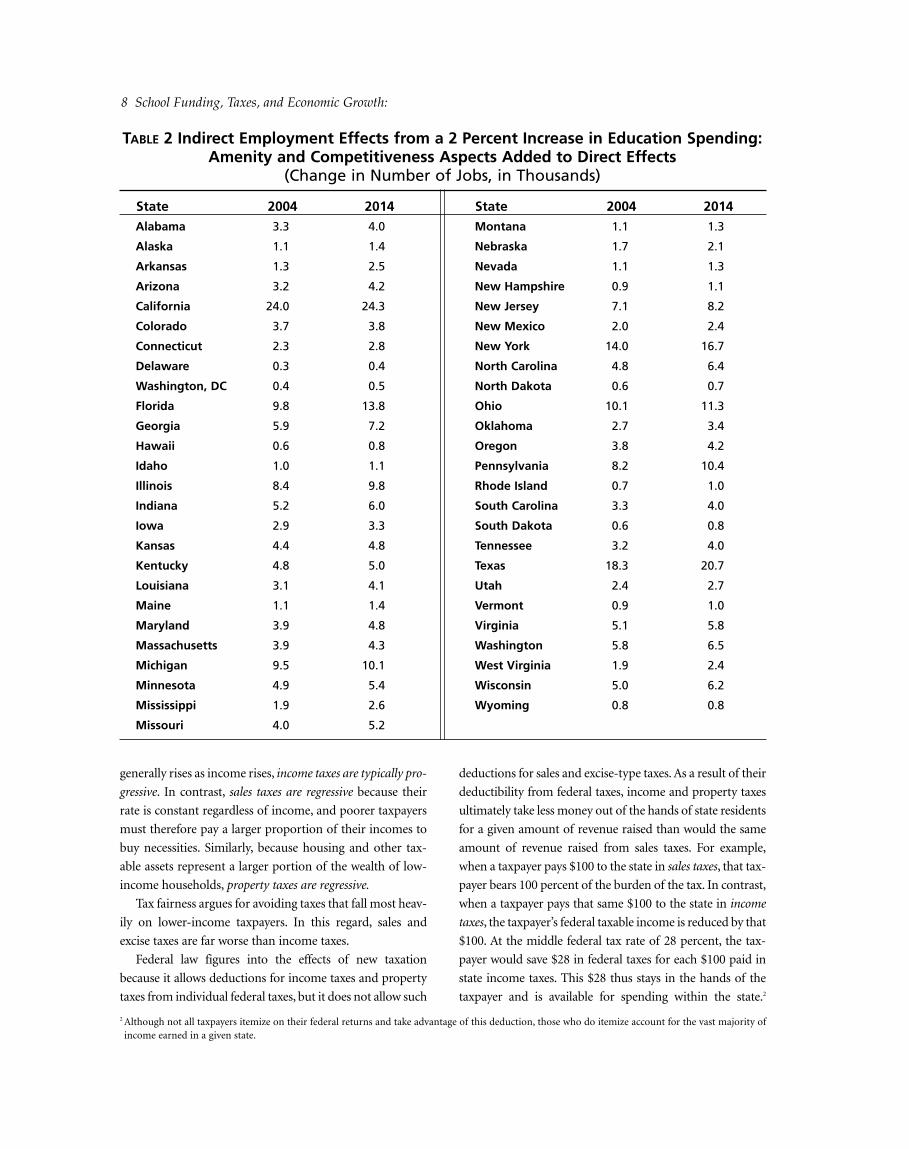
Incorporating the impacts of the amenity value of new
education spending along with the standard industrial
input-output impacts produces the results shown in Table
2. This table shows the effects on state employment when
the quality-of-life, or amenity, aspects of the increased edu-
cational effort are included. Adding amenities to the equa-
tion has relatively small near-term effects on the overall job
impact of the spending-and-taxing process. Over time,
however, as businesses and individuals make location deci-
sions and other adjustments in response to the higher qual-
ity of education, job growth continues to increase. The indi-
rect effects—the jobs resulting from the amenity and com-
petitiveness aspects—grow so that by the last year of the
analysis they are generally equal to, and for some states
greater than, the directs effects from education spending (as
can be seen by comparing the 2014 column in Table 2 with
that in Table 1).
Taxes: Paying the Piper
Because state and local governments must balance their
budgets, their additional spending requires an increase in
revenues, generally from an increase in taxes.1 As we
observed above, increased spending for education adds to
income and business activity within a region. Imposition of
new taxes has the reverse effect. That is, it reduces private
sector after-tax income, lowers demand for local goods and
services, and generally raises business costs.
The choice of a particular funding source for new spend-
ing—such as individual or corporate income taxes, sales or
excise taxes, or property taxes—has a different effect on the
state economy for a given amount of new taxes. The major
tax alternatives have somewhat different effects because they
place the burden on different components of the economy
and because federal law treats different taxes differently.
For example, increases in individual income taxes reduce
households’ disposable income, lower the returns from
working, and therefore reduce the supply of labor. Increases
in sales taxes increase the cost of goods and services, there-
by reducing what consumers can buy. Property taxes reduce
disposable income, lower the returns to asset ownership,
and reduce future investment in taxable property.
In addition, the burden of various state taxes falls differ-
ently on different taxpayers, according to their income lev-
els. Because the percentage of income paid in income taxes
1 Spending for one state program could come from a transfer of funding from other budget-supported activities, but, overall, new spending requires newrevenues.
8 School Funding, Taxes, and Economic Growth:
generally rises as income rises, income taxes are typically pro-
gressive. In contrast, sales taxes are regressive because their
rate is constant regardless of income, and poorer taxpayers
must therefore pay a larger proportion of their incomes to
buy necessities. Similarly, because housing and other tax-
able assets represent a larger portion of the wealth of low-
income households, property taxes are regressive.
Tax fairness argues for avoiding taxes that fall most heav-
ily on lower-income taxpayers. In this regard, sales and
excise taxes are far worse than income taxes.
Federal law figures into the effects of new taxation
because it allows deductions for income taxes and property
taxes from individual federal taxes, but it does not allow such
deductions for sales and excise-type taxes. As a result of their
deductibility from federal taxes, income and property taxes
ultimately take less money out of the hands of state residents
for a given amount of revenue raised than would the same
amount of revenue raised from sales taxes. For example,
when a taxpayer pays $100 to the state in sales taxes, that tax-
payer bears 100 percent of the burden of the tax. In contrast,
when a taxpayer pays that same $100 to the state in income
taxes, the taxpayer’s federal taxable income is reduced by that
$100. At the middle federal tax rate of 28 percent, the tax-
payer would save $28 in federal taxes for each $100 paid in
state income taxes. This $28 thus stays in the hands of the
taxpayer and is available for spending within the state.2
2 Although not all taxpayers itemize on their federal returns and take advantage of this deduction, those who do itemize account for the vast majority ofincome earned in a given state.
Alabama 3.3 4.0
Alaska 1.1 1.4
Arkansas 1.3 2.5
Arizona 3.2 4.2
California 24.0 24.3
Colorado 3.7 3.8
Connecticut 2.3 2.8
Delaware 0.3 0.4
Washington, DC 0.4 0.5
Florida 9.8 13.8
Georgia 5.9 7.2
Hawaii 0.6 0.8
Idaho 1.0 1.1
Illinois 8.4 9.8
Indiana 5.2 6.0
Iowa 2.9 3.3
Kansas 4.4 4.8
Kentucky 4.8 5.0
Louisiana 3.1 4.1
Maine 1.1 1.4
Maryland 3.9 4.8
Massachusetts 3.9 4.3
Michigan 9.5 10.1
Minnesota 4.9 5.4
Mississippi 1.9 2.6
Missouri 4.0 5.2
TABLE 2 Indirect Employment Effects from a 2 Percent Increase in Education Spending:Amenity and Competitiveness Aspects Added to Direct Effects
(Change in Number of Jobs, in Thousands)
State 2004 2014Montana 1.1 1.3
Nebraska 1.7 2.1
Nevada 1.1 1.3
New Hampshire 0.9 1.1
New Jersey 7.1 8.2
New Mexico 2.0 2.4
New York 14.0 16.7
North Carolina 4.8 6.4
North Dakota 0.6 0.7
Ohio 10.1 11.3
Oklahoma 2.7 3.4
Oregon 3.8 4.2
Pennsylvania 8.2 10.4
Rhode Island 0.7 1.0
South Carolina 3.3 4.0
South Dakota 0.6 0.8
Tennessee 3.2 4.0
Texas 18.3 20.7
Utah 2.4 2.7
Vermont 0.9 1.0
Virginia 5.1 5.8
Washington 5.8 6.5
West Virginia 1.9 2.4
Wisconsin 5.0 6.2
Wyoming 0.8 0.8
State 2004 2014
Taxes 9
Consequently, the impact on the state’s economy of selecting
a deductible versus a nondeductible tax is significant.
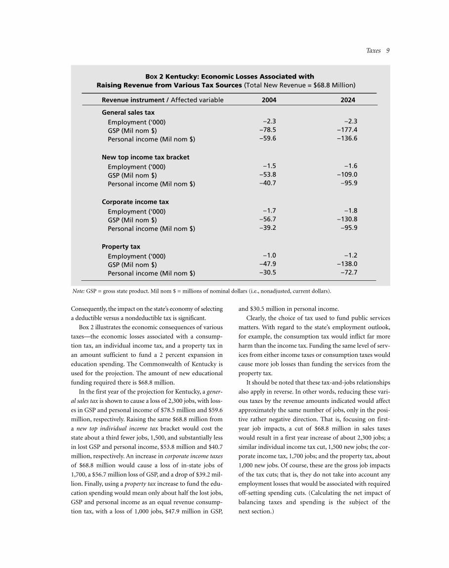
Box 2 illustrates the economic consequences of various
taxes—the economic losses associated with a consump-
tion tax, an individual income tax, and a property tax in
an amount sufficient to fund a 2 percent expansion in
education spending. The Commonwealth of Kentucky is
used for the projection. The amount of new educational
funding required there is $68.8 million.
In the first year of the projection for Kentucky, a gener-
al sales tax is shown to cause a loss of 2,300 jobs, with loss-
es in GSP and personal income of $78.5 million and $59.6
million, respectively. Raising the same $68.8 million from
a new top individual income tax bracket would cost the
state about a third fewer jobs, 1,500, and substantially less
in lost GSP and personal income, $53.8 million and $40.7
million, respectively. An increase in corporate income taxes
of $68.8 million would cause a loss of in-state jobs of
1,700, a $56.7 million loss of GSP, and a drop of $39.2 mil-
lion. Finally, using a property tax increase to fund the edu-
cation spending would mean only about half the lost jobs,
GSP and personal income as an equal revenue consump-
tion tax, with a loss of 1,000 jobs, $47.9 million in GSP,
and $30.5 million in personal income.
Clearly, the choice of tax used to fund public services
matters. With regard to the state’s employment outlook,
for example, the consumption tax would inflict far more
harm than the income tax. Funding the same level of serv-
ices from either income taxes or consumption taxes would
cause more job losses than funding the services from the
property tax.
It should be noted that these tax-and-jobs relationships
also apply in reverse. In other words, reducing these vari-
ous taxes by the revenue amounts indicated would affect
approximately the same number of jobs, only in the posi-
tive rather negative direction. That is, focusing on first-
year job impacts, a cut of $68.8 million in sales taxes
would result in a first year increase of about 2,300 jobs; a
similar individual income tax cut, 1,500 new jobs; the cor-
porate income tax, 1,700 jobs; and the property tax, about
1,000 new jobs. Of course, these are the gross job impacts
of the tax cuts; that is, they do not take into account any
employment losses that would be associated with required
off-setting spending cuts. (Calculating the net impact of
balancing taxes and spending is the subject of the
next section.)
BOX 2 Kentucky: Economic Losses Associated withRaising Revenue from Various Tax Sources (Total New Revenue = $68.8 Million)
Revenue instrument / Affected variable 2004 2024
General sales tax
Employment (‘000) –2.3 –2.3GSP (Mil nom $) –78.5 –177.4Personal income (Mil nom $) –59.6 –136.6
New top income tax bracketEmployment (‘000) –1.5 –1.6GSP (Mil nom $) –53.8 –109.0Personal income (Mil nom $) –40.7 –95.9
Corporate income tax
Employment (‘000) –1.7 –1.8GSP (Mil nom $) –56.7 –130.8Personal income (Mil nom $) –39.2 –95.9
Property tax
Employment (‘000) –1.0 –1.2GSP (Mil nom $) –47.9 –138.0Personal income (Mil nom $) –30.5 –72.7
Note: GSP = gross state product. Mil nom $ = millions of nominal dollars (i.e., nonadjusted, current dollars).

10 School Funding, Taxes, and Economic Growth:
Although state policymakers have the choice, at least in
principle, of using taxes such as income or property taxes
that would pass along a substantial part of the costs of
state spending to the federal government, most proposals
to increase state funding for education involve raising the
sales tax. Brunori (2001, pp. 597–98) found that of the five
education tax measures being considered, three involved
the sales tax, two the property tax, and none the income
tax. Poll results generally suggest as well that voters prefer
sales taxes to income or property taxes as ways of funding
any required new spending. For example, a recent poll in
New Jersey (Eagleton Poll 2003) found that 77 percent of
respondents thought that their state sales tax was “about
right,” and 61 percent answered that way about their
income tax, but only 25 percent said “about right” regard-
ing their property tax. Fully 50 percent said their property
tax was “much too high” compared with only 17 percent
answering that way for the income tax and 8 percent for
the sales tax.
Based in part on the current political reality that sales
taxes are the most likely source for new revenues, and in
part to illustrate the tax-and-spend effects using a “worst-
case” funding source, the present analysis uses a broad-
based general sales tax on all consumer goods as the
source of funding for the added educational expenditures.
Using any of the other major taxes as a funding source
should have a lesser negative impact on state employment
than does the consumption tax.
The results of increasing consumption taxes on each
state’s level of employment appear in Table 3. At this stage
of the analysis, tax revenues are simply being taken out of
the economy and not being respent. As would be expected,
Alabama –1.6 –1.8
Alaska –0.4 –0.6
Arkansas –0.1 –1.0
Arizona –2.0 –2.4
California –13.8 –13.3
Colorado –2.0 –2.0
Connecticut –1.1 –1.6
Delaware –0.1 –0.3
Washington, DC –0.2 –0.3
Florida –5.8 –7.0
Georgia –3.3 –3.8
Hawaii –0.3 –0.4
Idaho –0.3 –0.4
Illinois –4.5 –5.3
Indiana –2.7 –3.0
Iowa –1.3 –1.4
Kansas –2.2 –2.3
Kentucky –2.3 –2.3
Louisiana –1.7 –1.9
Maine –0.6 –0.7
Maryland –2.3 –2.5
Massachusetts –2.1 –2.3
Michigan –4.3 –5.1
Minnesota –2.7 –3.0
Mississippi –0.8 –1.1
Missouri –2.5 –2.9
TABLE 3 Employment Effects of an Increase in Consumption Tax Equivalent to 2 Percent of Education Spending (Change in Number of Jobs, in Thousands)
State 2004 2014Montana –0.5 –0.6
Nebraska –0.8 –1.0
Nevada –0.4 –0.7
New Hampshire –0.5 –0.6
New Jersey –3.4 –4.3
New Mexico –1.0 –1.1
New York –7.1 –8.6
North Carolina –2.8 –3.1
North Dakota –0.3 –0.3
Ohio –5.6 –6.0
Oklahoma –1.4 –1.7
Oregon –1.7 –1.9
Pennsylvania –5.3 –5.
Rhode Island –0.4 –0.5
South Carolina –1.5 –1.8
South Dakota –0.3 –0.3
Tennessee –1.8 –2.0
Texas –9.9 –10.4
Utah –1.1 –1.3
Vermont –0.4 –0.5
Virginia –2.7 –2.9
Washington –2.8 –2.9
West Virginia –0.7 –0.8
Wisconsin –2.7 –3.2
Wyoming –0.3 –0.3
State 2004 2014

Taxing and Spending 11
an increase in taxes affects jobs negatively in all states and
in all years. This negative effect on jobs increases over time,
as businesses and individuals continue to make location
decisions favoring areas offering greater opportunities.
Taxing and Spending: The Delicate Balance
The combined effects of an increase in education spending
and a general consumption tax (in a balanced-budget envi-
ronment) appear in Table 4. When all aspects of the added
K–12 education spending and the required consumer taxes
supporting that spending are considered, this analysis finds
that positive job growth occurs in all states and over all
future years. In every state, the job effects increase over
time, and in some states the effects in the last year of the
analysis, 2020, are substantially larger than in the initial
year. The difference in the state-to-state job growth rate is a
function of each state’s unique array of initial taxes, occu-
pational wage rates, industrial mix, self-supply of inputs,
and individual sensitivity to demand changes. The overall
impact is significantly positive for personal income in all
states in all years (see Appendix C).
What makes these job effects positive within a balanced-
budget fiscal policy? In the near-term, the positive effects
derive primarily from the fact that education spending is
(a) comparatively labor-intensive and (b) comparatively
local-supply intensive. On the first point, labor intensiveness,
consider that general consumer spending (i.e., other than
education), involves heavily capital-intensive items such as
Alabama 1.7 2.2
Alaska 0.7 0.9
Arkansas 1.2 1.5
Arizona 1.3 1.8
California 10.2 11.0
Colorado 1.7 1.8
Connecticut 1.2 1.3
Delaware 0.2 0.2
Washington, DC 0.2 0.2
Florida 4.0 6.7
Georgia 2.7 3.4
Hawaii 0.3 0.4
Idaho 0.7 0.8
Illinois 3.9 4.5
Indiana 2.5 3.0
Iowa 1.6 1.8
Kansas 2.2 2.5
Kentucky 2.5 2.7
Louisiana 1.3 2.2
Maine 0.5 0.7
Maryland 1.6 2.3
Massachusetts 1.8 2.0
Michigan 5.2 5.0
Minnesota 2.2 2.4
Mississippi 1.1 1.5
Missouri 1.5 2.3
TABLE 4 Net Effects of 2 Percent Education Funding and Matching Tax Increase with Educational Competitiveness Factors Considered
(Change in Number of Jobs, in Thousands)
State 2004 2014Montana 0.6 0.7
Nebraska 0.8 1.1
Nevada 0.7 0.6
New Hampshire 0.4 0.6
New Jersey 3.7 3.9
New Mexico 1.0 1.3
New York 6.9 8.1
North Carolina 2.0 3.3
North Dakota 0.3 0.4
Ohio 4.5 5.3
Oklahoma 1.3 1.7
Oregon 2.1 2.3
Pennsylvania 2.9 4.6
Rhode Island 0.4 0.5
South Carolina 1.8 2.3
South Dakota 0.4 0.5
Tennessee 1.4 2.0
Texas 8.4 10.3
Utah 1.3 1.4
Vermont 0.4 0.5
Virginia 2.4 2.9
Washington 3.0 3.5
West Virginia 1.2 1.5
Wisconsin 2.3 3.0
Wyoming 0.5 0.5
State 2004 2014

12 School Funding, Taxes, and Economic Growth:
automobiles, computers, appliances, and even food.
Typically, about 80 percent or more of school budgets are
for personnel costs. A given amount of spending on edu-
cation thus typically involves more labor and more per-
sonal income than does an identical amount of general
consumer spending. On the second point, the greater
local-supply intensiveness of education spending, consid-
er that purchases such as automobiles, televisions, elec-
tronic goods, and food as well as trips and vacations imply
substantial spending on out-of-state-produced goods and
services. State-funded public education spending on the
other hand, is heavily weighted toward in-state purchases,
not only for the main expenditure item of personnel but
also for goods and services.3
Over the longer term, the favorable impacts from
increased educational funding are largely attributable to
the effects educational support has on regional competi-
tiveness. Education spending is perceived in the market-
place as enhancing the quality of life in the affected area,
leading more people to move into the community. This
in-migration increases the labor supply in the area, mak-
ing the labor market more competitive, and it increases
the demand for locally produced goods and services.
Conclusions
This study finds that for state supported K–12 education
funding, the employment and economic effects of an
incremental increase in spending outweigh the losses asso-
ciated with the increased taxation in the near- and long-
terms. The positive net employment and economic effects
grow over time, as the enhanced educational spending
effort improves the perceived quality of life in the various
regions and as education-related productivity of the
regional workforce enables workers to command higher
earnings and makes businesses more profitable.
State-level decisions on public spending and taxation
clearly have significant implications for the regional econ-
omy and job creation, and both spending and taxation
must be carefully considered in making objective, accurate
evaluations. For the relatively small changes considered in
this analysis, education spending constitutes a significant
source of in-state jobs and economic growth, even consid-
ering the off-setting increases of a tax on local consump-
tion. The overall economic gains from education spending
increases arise from both the budgetary effects of educa-
tional spending in the near term and from the improve-
ments in regional competitiveness in the long term.
For the purposes of this analysis, a tax on consumer
spending is used as the funding source for the new educa-
tion spending. We noted earlier that consumption taxes
are highly regressive, because they impose a higher per-
centage of their burden on low-income households, and
that relying on alternative funding sources, such as income
or property taxes, would be more progressive and would
have less harmful economic effects. Unlike increased con-
sumption taxes (which among other things are not
deductible from federal taxes), federally deductible taxes
would decrease the local economic losses associated with
raising new tax revenues substantially.
Although these results are presented from the perspec-
tive of increases in spending and taxation, the results can
also be used as an approximation of the reverse case of
cutting education and taxes. For example, under the
assumptions of across-the-board education spending cuts
and a consumer spending tax cut, the resulting figures
would be approximately the same but in negative values.
In summary, when states confront the inevitable, difficult
decisions regarding public spending versus taxation, poli-
cymakers should bear in mind that both components of
the balanced-budget equation have implications for jobs
and income in the state. Policymakers should therefore
devote careful consideration to the likely results of those
specific decisions.
3 The present study is based on tax and spending changes made during periods of relative fiscal stability. Orszag and Stiglitz (2001) argued specificallythat during economic downturns, budget cuts have a more harmful effect on a state’s economy than do tax increases.

Appendix A: Education Expenditures ofState and Local Governments, by State
13
Alabama 3,570 71.4
Alaska 1,179 23.6
Arizona 4,085 81.7
Arkansas 1,999 40.0
California 29,890 597.8
Colorado 3,897 77.9
Connecticut 4,206 84.1
Delaware ,803 16.1
District of Columbia ,597 11.9
Florida 13,647 272.9
Georgia 7,858 157.2
Hawaii ,947 18.9
Idaho 1,178 23.6
Illinois 11,942 238.8
Indiana 5,967 119.3
Iowa 2,841 56.8
Kansas 2,827 56.5
Kentucky 3,441 68.8
Louisiana 3,773 75.5
Maine 1,303 26.1
Maryland 5,336 106.7
Massachusetts 6,066 121.3
Michigan 11,454 229.1
Minnesota 6,032 120.6
Mississippi 2,305 46.1
Missouri 5,180 103.6
TABLE A1 Direct General Expenditures of State and Local Governments forElementary and Secondary Education, by State ($ Millions)
State Actual 2% increaseMontana ,981 19.6
Nebraska 1,930 38.6
Nevada 1,510 30.2
New Hampshire 1,213 24.3
New Jersey 11,370 227.4
New Mexico 1,504 30.1
New York 26,188 523.8
North Carolina 6,382 127.6
North Dakota ,602 12.0
Ohio 11,896 237.9
Oklahoma 3,103 62.1
Oregon 3,596 71.9
Pennsylvania 12,549 251.0
Rhode Island 1,072 21.4
South Carolina 3,459 69.2
South Dakota ,673 13.5
Tennessee 4,254 85.1
Texas 20,130 402.6
Utah 2,096 41.9
Vermont ,661 13.2
Virginia 6,684 133.7
Washington 6,409 128.2
West Virginia 1,813 36.3
Wisconsin 6,303 126.1
Wyoming ,653 13.1
State Actual 2% increase
Source: U.S. Department of Commerce, Bureau of the Census (NCES 2000); Author’s calculations.

To determine the impacts of various fiscal policies
and economic proposals, the author used a set of
economic models of each state’s economy. The
modeling system, developed by Regional Economic
Models, Inc. (REMI), is a computable general equilibrium
model designed to simulate state and regional economic
and policy changes.4 Founded in 1980, REMI has devel-
oped and upgraded the model over time and currently has
users including state legislatures, state agencies, universi-
ties, regional planning agencies, national consulting firms,
utility companies, the U.S. Environmental Protection
Agency, and the National Institute of Standards and
Technology.
The model contains the economic linkages within the
state’s economy and allows the depiction of the conse-
quences of a wide range of policies and events for the
economy. It incorporates state-specific data along with
national economic trends and relationships to produce a
mathematical reproduction of the state economy.
To simulate the effects of a real-world change or devel-
opment, the model first states the change in the language
of economics, describing events in terms of their econom-
ic functions and implications. This language is precise and
sometimes subtle. For example, the model’s term increase
in output means that more of a good is produced, and,
because the local requirements for the good are
unchanged, the output is shipped outside the region. A
related term, increase in demand, means that local con-
sumers want more of the good but that local producers
will fulfill only a portion of that demand, and the remain-
der will come from outside the region. An increase in
demand may cause the price of the good to rise if the
model determines that the product is produced and used
primarily within the region.
Expressing events in terms of economic variables
allows careful and objective consideration of the event’s
impacts and implications.
The model is sensitive to a very wide range of policy and
project alternatives and to interactions between regional,
state, and national economies. It comprises explicit cause-
and-effect relationships, such as the following:
• Businesses use labor, capital, fuel, and intermediate
goods to produce output.
• Businesses change output in response to changes in
prices and costs.
• Supply and demand for labor depend on wage rates.
• The workforce expands when real after-tax wages rise
or the likelihood of being employed increases in a
region.
The cause-and-effect structure of the model allows
explanation of the results in terms of conventional eco-
nomic theory and relationships.
Simulations using the model begin by projecting a
baseline forecast for each state using historic trends and
relations and the expected outlook for the state and the
Appendix B: The Economic Model
4 Note: some descriptions of the REMI model are taken or adapted directly with permission from material supplied by REMI (see, e.g., REMI Web site,http://www.remi.com/overview/structure.html).
15

16 School Funding, Taxes, and Economic Growth:
nation. Policy changes that will affect this baseline forecast
can then be introduced using one or several of the more
than 8,000 variables in the model. The change can be in
the form of policy changes (e.g., increases or cuts in vari-
ous taxes, expansions or reductions in public programs, or
changes in regulations or standards) or market develop-
ments (e.g., an increase in demand for lumber, a rise in the
price of imported energy, a new aircraft engine assembly
plant, or an increase in the occupational training of the
local workforce). Any number of changes can be simulat-
ed at once. The initial changes introduced into the model
produce impacts on the region’s economic output; popu-
lation and labor supply; wages, prices, and profits;
demand for labor and capital; and local industry market
shares. Through the feedback responses in the model, each
of these induced impacts, in turn, produces further
impacts of its own, producing additional impacts, and so
on, until the economy returns to an equilibrium condi-
tion. Although the model does not strictly require a return
to equilibrium for any given period, it continually exerts
tendencies that push the results toward equilibrium. The
final results are presented as detailed changes in employ-
ment, income, population, and the demand for public
services in the area.
The data contained in the model are from original
sources, primarily the Bureau of Economic Analysis,
Bureau of Labor Statistics, Census Bureau, and U.S.
Department of Energy. For most series, the data history
extends back to 1969. The final results of the modeling
technique are a representation of the region’s economy
that predicts demand and supply conditions across 172
industry sectors, 94 occupations, 25 final-demand sectors,
and 202 age and sex categories.
A demographic component built into the model pro-
vides the ability to identify the changes in the workforce
and in the local population resulting from a simulation.
Changes in local employment opportunities, real wages,
living costs, and taxes lead to changes in the amount of
labor supplied in the region. Changes in the local labor
supply, in turn, lead to changes in the local population. An
initial increase in labor requirements would be met in part
by workers commuting into the region to pursue employ-
ment opportunities. Over time, a portion of these com-
muters and their families will move into the area, increas-
ing the local population and placing added demand on
public services. The model can produce detailed forecasts
of the state’s population by age, race, and sex.
The model incorporates forecasts of factor productivi-
ty and allows the option to modify the forecasts to accom-
modate policies that would change any of those produc-
tivities. Similarly, the model contains estimates of each
region’s relative amenity, or quality-of-life, values. These
amenity values, derived from heuristic analysis, are used to
explain why individuals and firms chose to locate in one
region as opposed to another when the directly measura-
ble economic factors were equal.
Model Structure
The structure of the model incorporates interindustry
transactions and endogenous final demand feedbacks. In
addition, the model includes substitution among factors
of production in response to changes in relative factor
costs, migration in response to changes in expected
income, wage responses to changes in labor market condi-
tions, and changes in the share of local and export markets
in response to changes in regional profitability and pro-
duction costs.
The power of the REMI model lies in its use of theo-
retical structural restrictions instead of individual econo-
metric estimates based on single time-series observations
for each region. The explicit structure of the model facili-
tates the use of policy variables that represent a wide range
of policy options and the tracking of the policy effects on
all the variables in the model.
The inclusion of price-responsive product and factor
demands and supplies give the REMI model much in
common with computable general equilibrium (CGE)
models. CGE models have been widely used in economic
development; public finance and international trade; and,
more recently, regional settings. Static CGE models usual-
ly invoke market clearing in all product and factor mar-
kets. Dynamic CGE models typically assume perfect fore-
sight intertemporal clearing of markets, or temporary
market clearing if expectations are imperfect. The REMI
model differs, however, because product and factor mar-
kets do not clear continuously. The time paths of respons-
es between variables are determined by combining a pri-
ori model structure with econometrically estimated
parameters.
Although the REMI model contains a large number of
equations, the five shaded blocks in Figure B1 describe its
underlying structure. Each block contains several compo-
nents, shown in rectangular boxes. The lines and arrows
represent the interaction of key components both within
and between blocks. Most interactions flow both ways,

Appendix B: The Economic Model 17
indicating a highly simultaneous structure. Block 1,
labeled output, forms the core of the model. An input-
output structure represents the inter-industry and final
demand linkages by industry. The interaction between
block 1 and the rest of the model is extensive. Predicted
outputs from block 1 drive labor demand in block 2.
Labor demand interacts with labor supply from block 3 to
determine wages. Combined with other factor costs, wages
determine relative production costs and relative prof-
itability in block 4, affecting the market shares in block 5.
The market shares are the proportions of local demand in
the region in block 1 and exogenous export demand that
local production fulfills.
The endogenous final demands include consumption,
investment, and state and local government demand. Real
disposable income drives consumption demands. An
accounting identity defines nominal disposable income as
wage income from blocks 2 and 4, plus property income
related to population and the cohort distribution of pop-
ulation calculated in block 3, plus transfer income related
to population less employment and retirement popula-
tion, minus taxes. Nominal disposable income deflated by
the regional consumer price deflator from block 4 gives
real disposable income. Optimal capital stock calculated in
block 2 drives stock adjustment investment equations.
Population in block 3 drives state and local government
final demand. The endogenous final demands, combined
with exports, drive the output block.
Model Application
The use of the REMI model for analysis of policy effects is
a two-step process, as shown in Figure B2. First, the model
generates a baseline forecast that uses a national forecast
as one of the inputs. Second, the direct effects of a policy
change are input into the REMI model to generate a fore-
cast for the local economy with the policy change (alter-
native forecast). The difference between the baseline and
alternative forecasts thus gives the total effects of a policy
change.
Direct effects of a policy change are input to the REMI
model through a large set of policy variables. They include
industry-specific variables, cohort-specific variables for 808
age-gender-race cohorts, and final demand-specific vari-
(1) Output
(4) Wages, prices, and production costs
State and local government spending
Investment Exports
OutputConsumption
Real disposable income
(2) Labor & capitaldemand
(3) Demographic (5) Market shares
Migration Population
Participationrate
Laborforce
Optimalcapitalstock
Employment
Labor/outputratio
Domesticmarketshare
Internationalmarketshare
Employment opportunity Wage rate Composite wage rate Production costs
Housing priceConsumer price
deflator Real wage rate Composite prices
FIGURE B1 Underlying Structure of the REMI Model
Source: Regional Economic Models, Inc., 306 Lincoln Ave. Amherst, MA 01002.

18 School Funding, Taxes, and Economic Growth:
ables for 25 final demand sectors. The policy variables cover
a wide range of possible types of inputs that make it possi-
ble to analyze any policy that may affect a subnational area.
Figure B3 shows how different types of policy variables
enter the REMI model through each of its five basic blocks.
Articles on Regional EconometricModels and the REMI Model
For readers who would like to pursue the details of econo-
metric modeling and the REMI model, a list follows of
further reading. The articles cited here are in four groups,
describing regional econometric models in general,
describing the REMI model in particular, evaluating the
REMI and similar regional policy models, and finally,
describing uses of the REMI model. Also included is an
overview of the REMI model structure and application.
Articles Describing Regional EconometricModels Generally
Almon, Clopper. 2001. The Craft of Economic Modeling.
5th ed. College Park: University of Maryland.
National Research Council. 1991. Improving Information
for Social Policy Decisions: The Uses of Microsimulation
Modeling. Vol. 1, Review and Recommendations, and
Vol. 2, Technical Papers. Washington, DC: National
Academy Press.
Schaffer, William A. 1999. Regional Impact Models.
Regional Research Institute, West Virginia University.
"What is the effect ofdecreasing electric rates?"
Policy Question
External Input
Decreased values forcommercial and industrialelectric rate policy variables and baseline values for all other external policy variables.
External InputBaseline value for all external policy variables.
Alternative Forecast1,975
1,769
year 1 year 2 year 3 year 4
Policy Effect1,975
1,769
year 1 year 2 year 3 year 4
Control Forecast1,975
1,769
year 1 year 2 year 3 year 4
REMI Model
FIGURE B2 Use of the REMI Model for Analysis of Policy Effects: A Two-Step Process
Source: Regional Economic Models, Inc., 306 Lincoln Ave. Amherst, MA 01002.

Appendix B: The Economic Model 19
Sims, Richard G. 2003. “Economic Modeling as an Aid to
Public Decision-Making.” In Jack Rabin, ed.,
Encyclopedia of Public Administration and Public Policy.
New York: Marcel Dekker.
Descriptions of the REMI Model
Treyz, G.I. 1993. Regional Economic Modeling: A
Systematic Approach to Economic Forecasting and Policy
Analysis. Norwell: Kluwer Academic Publishers.
Treyz, G.I., D.S. Rickman, and G. Shao. 1992. “The REMI
Economic-Demographic Forecasting and Simulation Model.”
International Regional Science Review 14(3): 221–53.
Articles Evaluating REMI and Similar Econometric Models
Brucker, Sharon M., Steven E. Hastings, and William R.
Latham III. 1990 “The Variation of Estimated Impacts
from Five Regional Input-Output Models.”
International Regional Science Review 13: 119–39.
DRI/McGraw-Hill. 1994. An Assessment of Input-Output
Models. Report prepared for the U.S. Department of
Transportation, New York.
Lahr, Michael L. 1996. “Comparison of Ready Made
Regional Economic Models in the U.S.” Paper given at
conference on Economic Impacts of Historic
Output
Supply Demand Market Shares
Wage Rates
Local and exportmarket sharesby industry
Wage rates, prices, and profits, by industry
Population by age, gender, race, and laborsupply
Employment demand byindustry andoccupation
Final demand by type and output by industry
FIGURE B3 Introduction of Policy Variables into the REMI Model
Source: Regional Economic Models, Inc., 306 Lincoln Ave. Amherst, MA 01002.

20 School Funding, Taxes, and Economic Growth:
Preservation, Rutgers University, Rutgers, N.J.
Rickman, D.S., and R.K. Schwer. 1995. “A Comparison of
the Multipliers of IMPLAN, REMI, and RIMS II:
Benchmarking Ready-Made Models for Comparison.”
Annals of Regional Science 29: 363–74.
Rickman, D.S., and R.K. Schwer. 1993. “A Systematic
Comparison of the REMI and IMPLAN Models: The
Case of Southern Nevada.” Review of Regional Studies
23(2, Fall): 143–61.
Articles Describing Uses of REMI
Braddock, David. 1995. “The Use of Regional Economic
Models in Conducting Net Present Value Analysis of
Development Programs.” International Journal of
Public Administration 18(1): 223–38.
Cassing, S., and F. Giarratani. 1992. “An Evaluation of the
South Coast Air Quality Management District’s REMI
Model.” Environment and Planning 24: 1549–64.
Lynch, T.M., P.J. Marsosudiro, M.G. Smith, and E.S.
Kimbrough. 1995. “The Use of Regional Economic
Models in Air Quality Planning.” International Journal
of Public Administration 18(1): 138–52.
Regan, Michael W., and Mark Prisloe. 2003. “Estimating
the Impact of Public Policy and Investment Decisions.”
Economic Digest 8(5, May): 1–6.

Appendix C: Detailed Results of 50-State Analyses
21
Alabama
Employment 1,671 1,808 1,830 2,266
Personal income (Mil nom $) 38 69 98 152
Alaska
Employment 687 717 719 856
Personal income (Mil nom $) 15 29 45 65
Arkansas
Employment 1,149 1,140 1,150 1,486
Personal income (Mil nom $) 21 38 57 92
Arizona
Employment 1,256 1,305 1,453 1,750
Personal income (Mil nom $) 24 57 83 142
California
Employment 10,610 11,390 10,050 11,150
Personal income (Mil nom $) 370 619 743 1,142
Colorado
Employment 1,663 1,505 1,612 1,798
Personal income (Mil nom $) 33 66 79 114
Connecticut
Employment 1,168 1,077 1,226 1,298
GRP (Mil fixed 92$) 8 4 (5) 10
Personal income (Mil nom $) 34 65 73 107
District of Columbia
Employment 155 126 138 148
Personal income (Mil nom $) 2 5 5 6
Delaware
Employment 207 194 170 179
Personal income (Mil nom $) 4 10 12 17
TABLE C1 Detailed Results of 50-State Analyses
State and economic measure 2004 2005 2010 2020
continues on next page

22 School Funding, Taxes, and Economic Growth:
Florida
Employment 4,047 4,972 6,624 7,295
Personal income (Mil nom $) 133 248 411 776
Georgia
Employment 2,674 2,711 3,139 3,466
Personal income (Mil nom $) 80 147 187 281
Hawaii
Employment 266 358 372 324
Personal income (Mil nom $) 7 14 19 29
Idaho
Employment 680 822 826 858
Personal income (Mil nom $) 17 30 43 61
Illinois
Employment 3,882 3,959 4,192 4,638
Personal income (Mil nom $) 125 218 257 385
Indiana
Employment 2,505 2,873 2,816 2,942
Personal income (Mil nom $) 54 100 130 190
Iowa
Employment 1,593 1,614 1,741 1,703
Personal income (Mil nom $) 32 56 75 105
Kansas
Employment 2,254 2,257 2,421 2,340
Personal income (Mil nom $) 22 42 58 88
Kentucky
Employment 2,485 2,515 2,721 2,768
Personal income (Mil nom $) 33 62 89 133
Louisiana
Employment 1,332 1,683 2,128 2,207
Personal income (Mil nom $) 41 74 108 166
Maine
Employment 425 448 568 657
Personal income (Mil nom $) 10 20 29 45
Maryland
Employment 1,580 1,670 2,285 2,443
Personal income (Mil nom $) 37 81 118 186
Massachusetts
Employment 1,818 1,860 1,939 2,107
Personal income (Mil nom $) 54 104 120 170
TABLE C1 Detailed Results of 50-State Analyses (continued)
State and economic measure 2004 2005 2010 2020

Appendix C: Detailed Results of 50-State Analyses 23
Michigan
Employment 5,154 5,512 5,080 4,517
Personal income (Mil nom $) 116 198 223 346
Minnesota
Employment 2,168 2,257 2,196 2,193
Personal income (Mil nom $) 53 98 116 172
Mississippi
Employment 1,108 1,233 1,318 1,534
Personal income (Mil nom $) 23 42 64 104
Missouri
Employment 1,504 1,998 2,290 2,198
Personal income (Mil nom $) 36 74 106 170
Montana
Employment 656 680 670 708
Personal income (Mil nom $) 12 21 30 44
Nebraska
Employment 848 854 840 946
Personal income (Mil nom $) 19 33 45 67
North Carolina
Employment 2,029 2,268 3,324 3,020
Personal income (Mil nom $) 59 111 159 255
North Dakota
Employment 337 344 337 346
Personal income (Mil nom $) 5 10 14 19
Nevada
Employment 655 549 625 676
Personal income (Mil nom $) 14 25 30 48
New Hampshire
Employment 347 452 552 608
Personal income (Mil nom $) 9 18 25 40
New Jersey
Employment 3,652 3,703 3,727 3,957
Personal income (Mil nom $) 106 186 227 335
New Mexico
Employment 972 1,133 1,279 1,219
Personal income (Mil nom $) 13 28 44 70
New York
Employment 6,864 8,659 8,130 8,993
Personal income (Mil nom $) 310 486 603 869
TABLE C1 Detailed Results of 50-State Analyses (continued)
State and economic measure 2004 2005 2010 2020
continues on next page

24 School Funding, Taxes, and Economic Growth:
Ohio
Employment 4,466 4,589 5,260 5,138
Personal income (Mil nom $) 104 197 244 370
Oklahoma
Employment 1,318 1,427 1,664 1,660
Personal income (Mil nom $) 30 54 76 117
Oregon
Employment 2,101 2,282 2,313 2,360
Personal income (Mil nom $) 46 80 107 158
Pennsylvania
Employment 2,880 3,972 4,612 4,810
Personal income (Mil nom $) 83 172 235 383
Rhode Island
Employment 393 394 451 457
Personal income (Mil nom $) 9 17 24 38
South Carolina
Employment 1,813 1,977 2,190 2,270
Personal income (Mil nom $) 39 72 103 156
South Dakota
Employment 364 468 471 508
Personal income (Mil nom $) 7 13 18 27
Tennessee
Employment 1,440 1,460 1,590 1,956
Personal income (Mil nom $) 45 76 102 164
Texas
Employment 8,400 9,664 10,281 10,371
Personal income (Mil nom $) 248 420 524 814
Utah
Employment 1,311 1,351 1,361 1,379
Personal income (Mil nom $) 23 45 57 78
Vermont
Employment 357 377 493 425
Personal income (Mil nom $) 6 12 18 26
Virginia
Employment 2,385 2,417 2,765 2,916
Personal income (Mil nom $) 56 107 141 209
Washington
Employment 3,047 3,150 3,348 3,577
Personal income (Mil nom $) 81 142 187 274
TABLE C1 Detailed Results of 50-State Analyses (continued)
State and economic measure 2004 2005 2010 2020

Appendix C: Detailed Results of 50-State Analyses 25
West Virginia
Employment 1,245 1,301 1,452 1,478
Personal income (Mil nom $) 24 41 61 93
Wisconsin
Employment 2,327 2,408 2,998 2,891
Personal income (Mil nom $) 57 107 140 216
Wyoming
Employment 471 499 498 494
Personal income (Mil nom $) 8 15 22 29
TABLE C1 Detailed Results of 50-State Analyses (continued)
State and economic measure 2004 2005 2010 2020
Note: GSP = gross state product. Mil nom $ = millions of nominal dollars (i.e., nonadjusted, current dollars).

Barro, Robert J. 2001. “Human Capital and Growth.”
American Economic Review 91(2, May): 12–17.
Bartik, Timothy J. 1992. “The Effects of State and Local
Taxes on Economic Development: A Review of Recent
Research.” Economic Development Quarterly 6(1
February): 102–10.
Betts, Julian R. 1995. “Does School Quality Matter?
Evidence from the National Longitudinal Survey of
Youth.” The Review of Economics and Statistics 77(2):
231–50.
Black, Sandra E. 1999.“Do Better Schools Matter? Parental
Valuation of Elementary Education.” Quarterly Journal
of Economics 114(May): 577–99.
Bogart, William T., and Brian A. Cromwell. 1997. “How
Much is a Good School District Worth?” National Tax
Journal 50: 215–32.
Bogart, William T., and Brian A. Cromwell. 2000. “How
Much is a Good Neighborhood School Worth?” Journal
of Urban Economics (March): 280–05.
Brasington, David M., 1999. “Which Measures of School
Quality Does the Housing Market Value?” Journal of
Real Estate Research 18(3): 395–413.
Brunori, David. 2000. “Good Politics—Tax Increases for
Schools.” State Tax Notes, February 21, 48.
Card, David, and Alan B. Krueger. 1996.“Labor Market
Effects of School Quality: Theory and Evidence.” In
Gary Burtless, ed., Does Money Matter? The Effect of
School Resources on Student Achievement and Adult
Success. Washington: Brookings Institution Press.
Crone, Theodore M. 1998. “House Prices and the Quality
Of Public Schools: What Are We Buying?” Business
Review, Federal Reserve Bank of Philadelphia,
(September/October): 3–14.
Dee, Thomas S. 2002. “The Capitalization of Education
Finance Reforms.” Journal of Law & Economics 43(1):
113–30.
Downes, Thomas A., and Jeffrey E. Zabel. 2000. “The
Impact of School Characteristics on House Prices:
Chicago 1987–1991.” Journal of Urban Economics 52:
1–25.
Eagleton Poll Archive. 2003. Scholarly Communication
Center, Rutgers University, January/February.
Retrieved February 2, 2004, from http://www.scc.rut-
gers.edu/eagleton/
Figlio, David N., and Maurice E. Lucas. 2000. “What’s in a
Grade? School Report Cards and Housing Prices.”
Working Paper 8019, National Bureau of Economic
Research, New York. November.
References
27
Note: For specialized bibliographic references on regional econometric modeling, see the section Articles on Regional
Econometric Models and the REMI Model, in Appendix B above.

28 K–12 Education in the U.S. Economy
Fisher, Ronald C. 1997. “The Effects of State and Local
Public Services on Economic Development.” New
England Economic Review (March/April): 53–62.
Florida, Richard. 2002. The Rise of the Creative Class and
How It’s Transforming Work, Leisure, Community and
Everyday Life. New York: Basic Books.
Garcia-Mila, Teresa, and Therese J. McGuire. 1992. “The
Contribution of Publicly Provided Inputs to States’
Economies.” Regional Science and Urban Economics 22:
709–38.
Goldin, Claudia, and Lawrence F. Katz. 2001. “The Legacy
of U.S. Educational Leadership: Notes on Distribution
and Economic Growth in the 20th Century.” American
Economic Review 91(2, May): 18–23.
Gradstein, Mark, and Moshe Justman. 2002. “Education,
Social Cohesion, and Economic Growth,” American
Economic Review 92(4): 1192–1204.
Hanushek, Eric A., and Dennis D. Kimko. 2000.
“Schooling, Labor-force Quality, and the Growth of
Nations.” American Economic Review 90(5, December):
1184–1208.
Haurin, D. R., and D. Brasington. 1996. “The Impact of
School Quality on Real House Prices:
Interjurisdictional Effects.” Journal of Housing
Economics (September): 957–71.
Hayes, Kathy J., and Lori L. Taylor. 1996. “Neighborhood
School Characteristics: What Signals Quality to
Homebuyers?” Federal Reserve Bank of Dallas,
Economic Review (Fourth Quarter): 2–9.
Helms, Jay. 1985. “The Effect of State and Local Taxes on
Economic Growth: A Time Series-Cross Section
Approach.” The Review of Economics and Statistics
67(4): 574–82.
Hilber, Christian A. L., and Christopher J. Mayer. 2002.
Do Households Without Children Support Local
Public Schools? Linking House Price Capitalization to
School Spending.” Wharton School Working Paper 02-
10, University of Pennsylvania, June.
Jacobson, Linda. 2002. “Poll: Public Sees Schools as a
Priority.” Education Week, April 24.
Jensen, Mark J., and Charles L. Leven. 1997. ”Quality of
Life Central Cities and Suburbs.” Annals of Regional
Science 31(4, September): 431–49.
Kahn, Matthew E. 1995. “A Revealed Preference Approach
to Ranking City Quality of Life.” Journal of Urban
Economics 38(2, September): 221–35.
Kane, Thomas J., Douglas O. Staiger, and Gavin Samms.
2003. “School Accountability Ratings and Housing
Values.” Brookings-Wharton Papers on Urban Affairs:
83–138.
Kodrzycki, Yolanda K. 2002. “Educational Attainment as a
Constraint on Economic Growth and Social Progress.”
In Education in the 21st Century: Meeting the Challenges
of a Changing World. Boston, MA: Federal Reserve
Bank of Boston. June.
Kotkin, Joe, and Ross C. DeVol. 2001. Knowledge-Value
Cities in the Digital Age. Los Angeles: Milken Institute.
February.
Margulis, Harry L. 2001. “Household Mobility, Housing
Traits, Public Goods, and School Quality in Cleveland’s
Metropolitan Statistical Area.” Urban Affairs Review
36(5, May): 646–77.
McGuire, Therese J. 2003 “Do Taxes Matter? Yes, No,
Maybe So.” State Tax Notes, June 9.
NCES (National Center for Education Statistics). 2000.
Digest of Education Statistics 2000. Table 34: Direct
general expenditures of state and local governments
for all functions and for education, by level and state:
1995–96. Retrieved January 27, 2004, from
http://www.nces.ed.gov/programs/digest/d00/dt034.ap
Nechyba, Thomas J. 2003. “What Can be (and What Has
Been) Learned from General Equilibrium Simulation
Models of School Finance?” National Tax Journal 56(2,
June): 387–414.
Orszag, Peter, and Joseph Stiglitz. 2001. “Budget Cuts vs.
Tax Increases at the State Level: Is One More Counter-
Productive than the Other During a Recession?” Center
on Budget and Policy Priorities, November 6.
Wasylenko, Michael. 1997. “Taxation and Economic
Development: The State of the Economic Literature.”
New England Economic Review (March–April): 37–52.
Weimer, David, and Michael Wolkoff. 2003. “School
Performance and Housing Values: Using Non-
Contiguous District and Incorporation Boundaries to
Identify School Effects.” National Tax Journal 56(2,
June): 231–54.
Yitzhaki, Shlomo. 2003. “Cost-benefit Analysis and the
Distributional Consequences of Government Projects.”
National Tax Journal 56(2, June): 319–36.