School Entry Policies and Skill Accumulation

Across Directly and Indirectly Affected Individuals

Kelly Bedard

Department of Economics

University of California, Santa Barbara

Elizabeth Dhuey

Centre for Industrial Relations and Human Resources

Department of Management

University of Toronto

September 2011

Abstract

During the past half century, there has been a trend towards increasing the minimum age a

child must reach before entering school in the United States. States have accomplished this

by moving the school entry cutoff date earlier in the school year: from January 1 towards

September 1. The evidence presented in this paper shows that these law changes increased

human capital accumulation and hence adult wages. Backing up the school entry cutoff by

one month (i.e. from January 1 to December 1) increases average male hourly earnings by

approximately 0.6 percent. Perhaps more importantly, the available evidence also suggests

that the majority of the cohort benefits from backing up the cutoff, not just those who must

delay entry.

We thank Sandra Black, David Card, Peter Kuhn, David Autor, Philip Babcock, and seminar

participants at the University of Calgary, UCLA, the University of Washington, UCSD, UC

Merced, the University of Manitoba, Tilberg University, Wilfrid Laurier University, the

University of Waterloo and the Society of Labor Economist Annual meetings for helpful

comments.

1

1. Introduction

What is the optimal age to start formal schooling? On one hand, the earlier children enroll in

school, the sooner they begin accumulating the skills taught there. On the other hand, enrolling a

child before he or she is ready for the academic rigors of formal education may be less

productive than waiting until that child is more mature. In addition, the presence of children who

are not yet ready for school may have a negative impact on the rate of human capital

accumulation among other students in the class, as teachers are forced to alter curriculum choices

and/or redirect resources towards these children. Despite the potential for offsetting effects, the

actions of policy makers suggest that they believe that students benefit from later school entry.

Early in the 20th century, most states allowed children to enter school in the fall as long as their

fifth birthday occurred before January 1 (Angrist and Krueger, 1991). Since the mid 1960s, 26

states have increased their minimum school entry age. In 1964, 18 states required children to turn

five on or before October 1, by 1988, 32 states had imposed this requirement (see Table 1).

State policymakers have enacted earlier school entry laws for a variety of reasons. First,

states with earlier cutoff dates have a higher average cohort age, which may improve school

readiness rates. Second, and perhaps more important to policy makers, backing up the cutoff date

means that cohorts are older when national assessments take place, which improves cross-state

relative test score rankings. Third, backing up the cutoff date generates a temporary reduction in

cohort size, and hence temporary cost savings. A recent policy study suggests that moving

California‘s cutoff date from December 2 to September 1 would save between $392 and $700

million dollars per year for the thirteen years that the smaller cohort attends public schools

(Cannon and Lipscomb, 2008).

2

While, to the best of our knowledge, there is no empirical research examining the overall

impact of school entry policies on student outcomes (both direct and indirect effects), there has

been a recent flurry of interest in the impact of school entry age on academic performance. The

usual approach is to use birth date variation relative to state-level school entry laws to estimate

the return to being relatively older within a cohort. Many studies find that children who are older

at school entry score higher on several important margins, ranging from better performance on

standardized achievement tests (Bedard and Dhuey, 2006; Datar, 2006; Elder and Lubotsky,

2009; Puhani and Weber, 2007; Smith, 2009; Crawford, Dearden, and Meghir, 2007), to higher

university enrollment rates (Bedard and Dhuey, 2006), to a higher probability of becoming a

high school leader (Dhuey and Lipscomb, 2008), to earning higher adult wages (Fredriksson and

Öckert, 2008; Kawaguchi, 2011). However, not all studies find long-term wage effects (Dobkin

and Ferreira, 2010; Fertig and Kluve, 2005; Black, Devereux, and Salvanes, 2011).

While parents are justifiably concerned about the impact of age at school entry, the

optimal minimum school entry age cutoff is the broader policy concern. In contrast to relative

age (or age at entry), which we have a limited ability to influence, given that all cohorts will have

an age continuum,1 we do have the ability to set public school minimum entry age laws.

Increasing the minimum entry age, by moving the cutoff date earlier in the year, has three

distinct effects.2 First, it increases the absolute age of directly affected children who must wait an

extra year before entering school due to the change in cutoff date. Second, it thereby increases

the average age of the entire cohort. Third, it increases the relative age of children who are

directly affected by the policy change and decreases the relative age of children who are not.

School entry law changes therefore have both a direct effect on the students affected by the

1 Although dual and multiple entry dates decrease relative age differences, these structures are rarely used.

2 Most school entry cutoff laws changes have moved the cutoff to earlier in the year. However, there are three cases

in which the cutoff has been moved to a later date (see Appendix Table 1).

3

policy change as well as spillover effects on their classmates who are not directly affected by the

policy change.

To give a concrete example, in 1973, New Mexico changed their school entry cutoff date

from January 1 to September 1. Before the law change, the youngest children entering

kindergarten were 56 months old (4 years and 8 months). After the law change, the youngest

entry age increased to 60 months.3 This entry law change therefore increased the average cohort

entry age from approximately 61.5 months to 65.5 months. While only children born between

September 1 and January 1 were directly affected by the policy change, children born during the

remainder of the year were indirectly affected by the increase in average starting age of their

cohort and the change in their location on the relative age scale. Our estimates encompass both

the effects on the directly and indirectly affected subsamples and should therefore be interpreted

as the average effect of the policy shift.4

Using a state of birth level repeated cross-section for 1959-1983 birth cohorts from the

2000 U.S. Census and the 2001-2007 American Community Surveys combined with school entry

laws from 1964-1988, we find that backing up the school entry cutoff by one month (i.e. from

January 1 to December 1) increases male hourly earnings by approximately 0.6 percent but has

little impact on average female hourly earnings. Given an ‗average‘ school entry change of about

3 months,5 this translates into a 1.8 percent increase in the average hourly earnings of males.

This is a sizeable increase and points to a substantial return for males to increased average age at

school entry within the entry cutoff range represented in the data, from September 1 through

January 1. As there are no school entry dates changes before September 1 during the period

3 This assumes that all children enter when eligible. We discuss early and late entry in Section 4.1.

4 In Section 5, we separately examine the effects for the directly and indirectly affected subsamples.

5 The unweighted mean school entry change is 2.7 months.

4

under study,6 it is an open question whether pushing the school entry cutoff date even farther

back would have a positive, negative, or neutral impact.

In an era in which backing up school entry dates is a popular potential education policy,

both because it involves short-term cost savings and because it is thought to improve inter-state

test score comparisons, it is important to point out that an average gain does not necessarily

imply that everyone gains. Directly affected individuals are forced wait a year to enter

elementary school and the labor market. Based on the male estimates reported in this paper, we

can approximate lifetime costs and benefits if we are willing to make strong assumptions about

labor market entry age, retirement age, the return to experience, the starting wage, and the

discount rate. For illustration purposes let us assume the following: labor market entry at age 20

with a starting wage of $25,000 per year, quadratic experience growth (0.02X-0.0003X2),

retirement at age 64, a 2 percent discount rate, and an extra $5,000 day care cost for children

who must wait an extra year to start school. Under these assumptions, the directly affected

individuals, those who must wait an extra year to enter school, suffer a lifetime wage loss if the

policy effect is less than approximately 4 percent because they must spend an extra year in

private cost childcare and they lose a year of employment (assuming that retirement age is

unaffected). At the same time, there is an overall gain to the cohort at large as long as the policy

effect is greater than approximately 0.35 percent. The gap between these estimates arises because

1/12 of the cohort pays the cost of policy change while 11/12 of the cohort only benefits from the

skill accumulation gain. The estimates reported in this paper suggest that the indirect effect is

6 The cutoff date in Missouri becomes August 1 in 1987 and July 1 in 1988. Since class sizes are also changing in

years with policy changes our specification includes state specific indicators for policy change years. Given this

specification and the fact that the only July and August policy change dates occur at the very end of the sample

period, with no cohorts following the policy change, our coefficient estimates for cutoff changes only reflect cutoff

changes between September and January. See Section 2.

5

approximately 1 percent, therefore there appears to be a small loss to directly affected

individuals and a substantial gain for the majority of the cohort.

2. The Impact of Minimum School Entry Age Laws

Since the innovative work of Angrist and Krueger (1991), who use quarter of birth as an

instrument for educational attainment,7 many researchers have used birth dates and school entry

and exit laws in somewhat modified ways. Prominent examples include Lleras-Muney‘s (2005)

examination of the impact of education on adult mortality using compulsory schooling and work

laws to instrument for educational attainment. Oreopoulos, Page and Stevens (2006) use the

same IV strategy to estimate the impact of parental education on offspring schooling outcomes.

In addition, McCrary and Royer (2011) use a regression discontinuity design in California and

Texas to compare the fertility outcomes of women born just before and just after the school entry

cutoff date. Finally, Oreopoulos (2006) and Clark and Royer (2010) use the increase in the

national compulsory law in the U.K. in 1947 to estimate the impact of educational attainment on

earnings (Oreopoulos, 2006) and health and mortality (Clark and Royer, 2010).

However, the results from the literature using school entry laws referenced in the

introduction along with the literature on school exit laws draws into question the use of quarter

of birth and compulsory schooling laws in instrumental variable, state panel, and regression

discontinuity frameworks, at least in the U.S. context.8 There are two key issues. First, if relative

age within a cohort directly affects human capital accumulation as well as affects educational

attainment, it likely has a direct impact on other outcomes. Therefore, using school entry laws as

7 See Bound, Jaeger and Baker (1995), Bound and Jaeger (2000), and Dobkin and Ferreira (2010) for detailed

discussions of the pros and cons of using quarter of birth as an instrument for educational attainment. 8 There is no evidence to suggest that the compulsory schooling change(s) used by Oreopoulos (2006) and Clark and

Royer (2010) are invalid.

6

instruments is invalid. Second, if compulsory schooling laws change educational attainment,

discontinuities in educational attainment should be localized near the binding cutoffs. However,

they appear over a range of high school grades, which leads one to wonder if it is really the

interaction between school entry and exit laws that are driving the observed educational

attainment differences (see Dobkin and Ferreira, 2010).

None of this, however, changes the fact that school entry and/or exit laws may have an

important impact on human capital accumulation. Rather, it suggests that there may be multiple

interacting effects associated with such laws. Minimum school entry age (cutoff) laws impact

student outcomes in at least two important ways. First, and most obviously, they determine age at

school entry: A January 1 cutoff implies a school entry age range of 56 to 67 months,9 while a

September 1 cutoff implies an entry age range of 60 to 71 months. Second, while only children

born between September 2 – December 31 are forced to wait an extra year before entering school

under the September 1 cutoff compared to the January 1 cutoff, the other children in each school

entry cohort are indirectly affected by the increase in average starting age and a change in their

relative age position within the cohort.

It is easiest to discuss the implications for the directly affected group first. Since this

group waits an extra year before entering school, there are three inter-related age effects. First,

they are a year older when they enter school, which may increase their level of school readiness

(see Stipek, 2002, for a review of the literature). While the rhetoric surrounding cutoff date

changes suggests that it is widely believed that children have more rapid human capital

accumulation if they enter school at older ages, theoretically, the impact is ambiguous and it is

therefore an empirical question. In addition to becoming absolutely older, directly affected

children also become relatively older; they switch from being the youngest children in their

9 For descriptive ease, we assume that all children enter when eligible, we will return to this issue.

7

cohort to being the oldest children in their cohort. The findings from the age at school entry

literature suggest that this aspect of the entry law change will have a positive, or at worst zero,

impact on directly affected children. Third, the entire cohort is now older. To the extent that

younger school—unready classmates have a negative impact on the entire class, postponing the

enrollment of these individuals by a year may have a positive impact on the entire cohort. Since

all of these effects are non-negative, with the possible exception of the absolute age effect, one

may expect a positive net effect for the directly affected subgroup. It is worth pointing out,

however, that these effects are not separately identifiable because the relative age and the cohort

age changes add up to the absolute age change for directly affected individuals.

In contrast, the net effect for the indirectly affected group is less complicated, but of

ambiguous direction. Since school entry age is unchanged for this group, the net effect has only

two components. Just as for the directly affected group, the entire cohort is older. As discussed

above, this should have a positive impact. On the other hand, this group is now relatively

younger. For example, children born in January switch from being the relatively oldest in their

cohort under a January 1 cutoff to a more middle position in the relative age distribution under a

September 1 cutoff. At the same time, children born in August move from the middle of the

relative age distribution to the relatively young end. Since the relative age and average cohort

age effects may go in opposite directions, the net effect is ambiguous for indirectly affected

children.

While the net effect for certain subgroups within school entry cohorts are theoretically

ambiguous, the average cohort effect is likely positive. We conjecture this because of the likely

positive absolute age effect for directly affected students, the likely positive average cohort age

8

effect for the entire cohort,10

and the fact that the relative age effects wash out on average.11

While the overall effect is therefore likely to be positive, there is no unambiguous prediction,

rendering both the sign and the magnitude an empirical question.

The primary objective of this paper is to estimate the overall policy impact. More

specifically, we estimate the net, or average, effect of changing the minimum school entry age.

We do this using a state of birth level repeated cross-section. Since age at school entry and the

peer effects associated with cohort age composition can affect skill accumulation either directly

through within grade human capital accumulation rates or through educational attainment, the

most natural way to think about estimating the impact of minimum school entry age laws on

adult earnings is as follows:

ibtybtbibtyibtybtibty TBAXSW 543210 (1)

where ibtyW denotes the ln adult wage, for individual i born in state b in year t observed in Census

or American Community Survey year y, btS denotes the age at which the youngest member of the

cohort is eligible for kindergarten in birth state b in birth year t, ibtyX is a vector of race indicators,

state of birth specific indicators denoting that it is the year of, before or after an entry age policy

change,12

and in most specifications birth state specific education institution and quality

controls,13

ibtyA is a vector of age indicators, bB is a vector of state of birth indicators, btT is a

10

Note that the first two effects are not separately identifiable since they move together. 11

While different students may be relatively older or younger, there is always a 12-month age range. Years in which

the cutoff changes are exceptions: The age range is shorter in these years. 12

This indicator allows for the fact that years surrounding entry age law changes also have cohort size changes. If

everyone enters on their legally defined date, every month that the school cutoff moves back implies a 1/12

reduction in the cohort size for the first year of the cutoff change. As leads and lags are often associated with law

changes, it is also possible that the years preceding and following changes also experience cohort fluctuations.

Including controls for these years ensures that we do not confound cohort size and entry age effects. 13

This includes kindergarten subsidization, pupil teacher ratio, relative teacher salaries, and compulsory school

leaving age. See Section 3.3 for details.

9

vector of census region of birth specific cohort indicators, and ibty is the usual error term.14

Notice that equation (1) does not hold educational attainment constant since school entry laws

may change skill accumulation through either within grade human capital accumulation or

through educational attainment. All models are population weighted and the standard errors are

clustered at the state of birth level.

It is worth re-emphasizing that the reduced form estimate of the effect of the minimum

school starting age on earnings described by equation (1) is the average effect of the policy on

the entire birth cohort. In other words, it is the overall average impact of a change in the

minimum school starting age, as opposed to the average impact of the policy on just those

children whose school entry are delayed by the change in the minimum school starting age. It

also is important to note that 1 is also net of changes in parental decisions regarding early and

late entry. If all parents simply enrolled their children as soon as they became eligible we would

observe exactly the correct fraction of each month or quarter of birth enrolled in school at age

five. However, some parents enroll their child a year early and some hold them back and enroll

them a year late. To the extent that these decisions are sensitive to cutoff dates, the reduced form

estimate is net of this. In particular, if backing up the cutoff date means that fewer children born

in the fall are voluntarily held out of school for a year by their parents then 1̂ will be smaller

than might be expected since there is less change in cohort composition than predicted as these

children were already ―conforming‖ to the new cutoff even before it existed. In the same vein,

backing up the cutoff may also induce some parents to switch from on-time entry to early entry,

which will again reduce the estimated effect since it again amounts to no change in observed

behavior. We will return to this issue in Section 4.1.

14

Alternative specifications are explored in Sections 4 and 5.

10

3. Data

3.1 School Entry Laws

In most states, a statewide statute or regulation mandates the age at which children are eligible to

enter primary school. For example, a child can enter school in California as long as the child

turns five by December 2 of that academic year. For descriptive ease, Table 1 reports the number

of states by cutoff month in 1964 and 1988. For example, the first row reports the number of

states that have a cutoff date of January 1 or February 1. This means that children need to reach

age five before January 1 or February 1, respectively. The last two rows report the number of

states that leave school entry to the discretion of local education authorities or have no school

entry law, respectively. Table 1 reveals a clear pattern: states have been backing up their school

entry laws over time forcing children to be older before entering the education system. In 1964, 8

states required children to be five by September but by 1988, 21 states had this requirement. The

complete set of entry laws from 1964-1988 are reported in Appendix Table 1.

All school entry cutoff dates were collected from state statutes and corresponding

historical state session laws and/or regulations. The current list of statutes with citations can be

found in Appendix Table 2. In addition, Appendix Table 3 lists the cutoff date in each state in

1964 with its corresponding legal citation regarding this cutoff date in 1964. The table then lists

the year of change, if any, what the new cutoff date is and the legal citation, which indicates the

changing of the cutoff date. A legislative history of each statute from 1964-1988 is available

from the authors upon request.15

15

These cutoff dates have been cross-referenced with Angrist and Krueger (1992), Cascio and Lewis (2006), the

Digest of Education Statistics (1972, 1973, and 1983), the Educational Research Service (1975), and information

from the website of the Education Commission of the States (http://www.ecs.org). Some conflicting cutoff date

information exists between sources. It is unclear why the dates differ but if our cutoff date differed from a

previously published source, we re-checked the legislative history for the statute. If the dates differ, we list the date

indicated in the statutes and corresponding historical state session laws for that particular year. See Appendix Tables

2 and 3 for more details regarding citations.

11

In order to simplify the coding of dates, all entry laws are coded as either the first of the

month or mid-month. This avoids confusion between end of month and beginning of month

differentiation and inconsequential law changes of one or two days.16

States that do not have

statutes or regulations regarding their entry law during a particular time period are reported as

none during those years in Table 1 and Appendix Table 1 and are coded as missing in the data.

States that leave school entry at the discretion of local authorities are also coded as missing in the

data since we do not have sub-state level information. Lastly, states requiring children to be five

years old by the start of the school year in order to enroll are coded as a September 1 cutoff.17

Estimating equation (1) requires that we restrict attention to the subset of years reported

in Appendix Table 1 (cohorts who are age five in 1964-1988). We use these cohorts because we

need to calculate the age at which the youngest member of the cohort is eligible for school entry

and link the cohort to adult wages later in life. As will be discussed in detail in the next section,

the best available wage data come from the 2000 U.S. Census and the 2001-2007 American

Community Surveys. Unless otherwise stated, all analyses use state school entry cutoffs from

1964-1988. This translates into using the entry cutoff dates for 1959-1983 birth cohorts.

3.2 Wages

In order to match people to the school cutoff in place when they were entering school, we assign

cutoffs to individuals based on the law in place in the state of birth when their ‗cohort‘ was 5

years old. Since quarter of birth is only available for the 2005-2007 ACSs—the census and the

2001-2004 ACS only report age as of April 1—we assign people to age 5 cohorts using year–

16

This simplification has no substantive effect. 17

The one exception is Montana, which is coded as mid-September because they list September 10th

as the school

entry cutoff date beginning in 1979, and it does not appear that this was a change in policy from the previous

regime.

12

age+4. While this incorrectly assigns some people, it is the best that we can do without more

detailed birth date data.18

Ideally, one would restrict attention to individuals who have completed all major

schooling and who are pre-retirement. For example, by restricting the sample to individuals aged

of 30-54. However, most of the cutoff changes occurred recently–there are only seven cutoff

changes between 1964 and 1975. Since it is important to use the most recent cohorts possible, we

restrict the sample to U.S. born individuals from the 1959-1983 birth cohorts in the 2000 U.S. 5

percent Public Use Micro Census and the 2001-2007 American Community Survey (ACS). The

ACS is a nationally representative annual 1 in 250-person sample of the United States. This

choice of sample allows the use of 20 statewide cutoff changes. Using the ACS has two

important advantages. First, it increases the available data for young cohorts surrounding cutoff

changes. Second, the addition of a year of observation dimension allows us to control for age and

birth cohort separately.

The drawback to focusing on the cohorts who were eligible to enter kindergarten from

1964 through 1988 is that wage observations are at younger than optimal ages for the later

cohorts. The sample includes people aged 23-45 who reside in the 48 contiguous states.19

This

choice is a tradeoff between two factors. On one hand, we would prefer to focus on wages after

age 30 when we are more confident that educational investments are largely complete. On the

18

In our case, incorrect cohort assignment is only a serious problem in years with policy changes. The inclusion of

state of birth specific policy year indicators is therefore important. We also check the robustness of our results by

dropping observations for the year before, of, and after a change in our base specification. The results are similar in

all cases. Our specification has four additional benefits. (1) It is appropriate in cases where there are leads or lags in

adoption. (2) It eliminates policy-timing difficulties associated with states in which school entry is grade one rather

than kindergarten. (3) As discussed in footnote 12, it ensures that we are not confounding entry age law changes

with changes in cohort size in the years immediately surrounding cutoff changes. (4) It mitigates problems

associated with the miss-match caused by allocating individuals to birth cohorts based on age rather than based on

school year cohorts because the miss-allocation only miss-assigns school entry policies in the years directly

surrounding changes. While cohort assignment based on school years rather than age does not suffer from the miss-

allocation problem, it is impossible to implement because we do not have exact birth dates. 19

Observations with imputed education, wage, sex, race, or place of birth data or missing education information are

excluded from the sample.

13

other hand, this would require excluding the post-1976 birth cohorts, which means losing a

quarter of the cutoff changes as well as losing more than half the wage observations surrounding

another quarter of the cutoff changes. Given these data limitations, we focus on employed young

adults, ages 23-45.

Table 2 summarizes the Census and ACS data. It reports summary statistics for U.S. born

men and women under the two different sample definitions used in this analysis. Column 1 and 3

report the summary statistics for all males and females. These samples are used to examine the

impact of cutoff changes on educational attainment. Columns 2 and 4 are restricted to males and

females who are not in school or prison and who work for wages (are not self-employed) and

report positive income. These are the primary samples used in the majority of the analysis.

3.3 Other Education Policy Controls

The identification of the model comes from state-time variation in minimum school entrance

ages induced by statewide school entry policy changes. If cutoff changes tend to be bundled with

other policies that affect academic and hence labor market outcomes, it is important to control

for these in equation (1). While we are aware of no evidence of other policies being bundled with

cutoff date changes, we control for school exit laws, pupil-teacher ratios, teachers salaries, and

the beginning of state subsidized kindergarten.

The pupil-teacher ratio is the number of students in each state divided by the number of

teachers. Birth cohorts are assigned the average pupil-teacher ratio during their thirteen years of

available public schooling. Relative teacher salaries are defined as the average wage of teachers

divided by the average wage of 30-49 year old male BA holders in the 1950-2000 U.S. Censuses

(inter-census years are linearly interpolated). The number of students, the number and the wages

14

of teachers, and the oldest age required by compulsory schooling laws are from the Digest of

Education Statistics. Information not provided by the Digest of Education Statistics regarding the

oldest age required by compulsory schooling are from state statutes and corresponding historical

session laws. The small number of cases with missing student and teacher counts and wages are

linearly extrapolated. The beginning of state subsidized kindergarten is an indicator variable for

whether states subsidized kindergarten with state revenue in a particular state for a particular

birth cohort.20

4. Short-Run Effects of Minimum School Entry Age Laws

While our ultimate goal is to examine the impact of minimum school entry age laws on adult

earnings, the existence of such effects depends on compliance with law changes. Before turning

to the wage estimates, we therefore examine the available evidence on compliance with school

entry date cutoff changes.

4.1 Do Minimum School Entry Age Laws Change School Entry?

Compliance with minimum school entry age law changes is imperfect because parents and/or

educators can advance or delay school entry for specific children. Acceleration and deferral

usually require petitioning the school or district for an exception. While in recent years it is rare

for children to enter school early, it was more common in the past.21

For example, in 1980, 8

percent of children born in the fourth quarter of the year in Minnesota were enrolled in

kindergarten even though the official cutoff date was September 1. At the same time, 5 percent

of the children born in the first quarter of the year from the same cohort were not enrolled in

20

See Dhuey (2011) for information regarding collection of data on state subsidized kindergarten. 21

Using data from the Early Childhood Longitudinal Study, Kindergarten Class of 1998-99, only 1.8 percent of

children entered kindergarten early in the 1998 school year.

15

kindergarten, even though according to the minimum school entry laws they were eligible. In

contrast, in Maryland, 87 percent of fourth quarter children were enrolled in kindergarten in

1980, which means that 13 percent deferred entry given the January 1 cutoff date.

We estimate the impact of changes in minimum school entry age laws on school

enrollment using data on six year olds22

residing in the 48 contiguous states that have state-level

minimum school entry laws in the 1960, 1970 and 1980 U.S. Censuses23

using the following

slightly simplified version of equation (1).

iryryriryryiry YRXSE 43210 (2)

where iryE is the enrollment status (1 = enrolled in first grade or higher)24

of child i in state of

residence r in census year y, ryS denotes the age at which the youngest member of the cohort is

eligible for school entry, iryX is a vector of race indicators and an indicator for the availability of

publically subsidized kindergarten, rR is a vector of state of residence indicators, ryY is a vector

of census region specific year indicators, and iry is the usual error term. All models are

population weighted and the standard errors are clustered at the state level.

The equation (2) results are reported in Table 3. The results for males are reported in

columns 1-4 and the results for females are reported in columns 5-8. Focusing on column 1 and

5, backing up the school cutoff date by one month decreases the fraction of six year olds enrolled

in grade one or higher by 3.4 percentage points and backing it up by three months decreases

enrollment by 10.2 percentage points, for both males and females. If the entire impact comes

22

We focus on enrollment in first grade rather than kindergarten for two related reasons: (1) kindergarten enrollment

is not compulsory in most states during this time period, and (2) some states have low kindergarten enrollment rates

during this period, at least partly due to kindergarten not being subsidized with state revenue. 23

Cohorts are defined by age rather school year due to data limitations. All results are similar if we define cohorts

based on the calendar year instead of age. 24

The results are almost identical if we define enrollment status as 1 if enrolled in grade 1.

16

from those directly affected by the cutoff change, this implies a compliance rate of

approximately 40 percent. These findings of imperfect compliance are consistent with Dobkin

and Ferreira (2010). The large discrepancy reflects the fact that children with birthdates near

cutoffs are more likely to be accelerated or retained.

Unlike the majority of the available wage data, the 1960, 1970 and 1980 Census data

includes quarter of birth information. This allows us to see whether changes in enrollment are

driven by groups directly affected by cutoff date changes. More specifically, since all cutoff

changes during this period occur between January 1 and September 1, most of the enrollment

change should be driven by children born in the fourth quarter, with a small impact on third

quarter children. We therefore generalize equation (2) to allow differential effects across

quarters. In particular, indicators for first, second and third quarter births and their interactions

with S, R, and Y are added to the model. This specification allows the impact of cutoff changes to

differ across birth quarters. The results for the generalized model are reported in columns 2 and 6

in Table 3 for males and females, respectively. Focusing on these columns, backing up the

school cutoff date by three months decreases the fraction of fourth quarter six year old males

(females) enrolled in grade one or higher by 39.6 (42.3) percentage points, reduces enrollment

among third quarter babies by 5.7 (5.1) percentage points, and has no measurable impact on

enrollment for first and second quarter six year olds. As a final specification check, columns 3, 4,

7, and 8 add linear state trends. The results are robust to the inclusion of this trend specification

in all cases.25

25

Appendix Table 4 generalizes the Table 3 models by adding interactions between race/ethnicity and btS . This

exercise reveals some evidence that black and Hispanic students are less likely to reduce enrolment in response to a

law change.

17

4.2 Educational Attainment

While it is not necessary for cutoff changes to effect educational attainment in order to have an

impact on labor market outcomes, given the possible direct impact on skill accumulation, it is

nonetheless useful to examine the possible educational attainment effects before estimating the

effect on wages. The most natural way to think about estimating the impact of school entry age

on educational attainment follows directly from the specification of the basic wage model

described by equation (1) in Section 2.

ibtybtbibtyibtybtibty TBAXSEd 543210 (3)

where ibtyEd denotes the attainment of a specified level of education, for individual i born in state

b in year t observed in Census or ACS year y, btS denotes the age at which the youngest member

of the cohort is eligible for school entry in birth state b in birth year t, ibtyA is a vector of current

age indicators, bB is a vector of state of birth indicators, and btT is a vector of census region of

birth specific cohort indicators. In the baseline specification (columns 1 and 6 in Tables 4 and

5), ibtyX includes race and state of birth specific indicators for it being the year of, before, or after

a policy change.26

Columns 2 and 7 expand ibtyX to include the availability of publicly subsidized

kindergarten, the pupil teacher ratio, relative teacher salaries, and the compulsory school leaving

age.

While the most reduced form approach is to exclude later life controls, such as marital

status and factors that depend on current residential location, as they may all be endogenous to

the policy change of interest, we nonetheless check the robustness of our results to a variety of

additional controls. The model reported in columns 3 and 8 add a vector of state of residence

26

The policy year indicators are state of birth specific because states changed school entry dates by different

amounts.

18

indicators, a vector of census region of residence specific age indicators, cohort size defined by

state of birth, state of residence specific GDP and unemployment rates,27

and marital status. The

model in columns 4 and 9 further adds a set of region of birth–region of residence interactions to

control for selective migration. Heckman, Layne-Farrar, and Todd (1996) show that non-random

migration across regions may confound education policy point estimates. We follow their

approach and check the sensitivity of our results to including a matrix of region of birth and

region of residence interactions that control for migration choices. Finally, columns 5 and 10 add

state of birth specific linear cohort trends.

Table 4 reports the educational attainment results using equation (3) for men and women

aged 23-45 in the 2000 U.S. Census and the 2001-2007 ACSs. The first row reports the

estimated impact of a one-month moving back of the school start date earlier in the year on the

probability of graduating from high school. Rows 2 and 3 similarly report the probability of

obtaining some college or more and obtaining an undergraduate degree or more. There is little

evidence that school start dates impact educational attainment at any level. As such, any

substantive impact on wages must be coming through changes in within grade skill

accumulation.

5. The Long-Run Effect of Minimum School Entry Age Laws on Adult Wages

The baseline equation (1) ln hourly wage estimate for men is reported in row 1 of column 1 in

Panel A of Table 5. The sample includes men aged 23-45 in 2000-2007 who are not in prison or

school and work for wages and report positive income. Similar to Table 4, columns 2-5

progressively expands the set of control variables for the male models. Column 2 adds a set of

27

State GDP data are from the Bureau of Economic Analysis and are reported in 2007 dollars. State unemployment

rates are from the Bureau of Labor Statistics.

19

education quality variables. Column 3 adds state of residence, census region of residence specific

age indicators, cohort size defined by state of birth, state of residence specific GDP and

unemployment rates, and marital status. Column 4 further adds an interaction between region of

birth and region of residence and Column 5 adds linear state of birth specific cohort trends.

Depending on the specification, we estimate that a one-month increase in the minimum school

starting age increases average male hourly wages by 0.55-0.68 percent. Using the mean cutoff

change of 3 months, this range translates into a 1.65-2.04 percent increase in average male

hourly wages.

The same set of results for women is reported in columns 6-10. While the female point

estimates are generally smaller, the male-female difference is not always statistically significant.

More specifically, the results indicate that a one-month increase in the minimum school starting

age is associated with a 0.21-0.47 increase in the average female hourly wage, which translates

into a 0.63-1.41 percent increase for a 3-month entry age change. There are two important

caveats. First, not all female coefficients are precisely estimated: We cannot reject the null

hypothesis of no effect even at the 10 percent level for the specifications reported in columns 6

and 7. Second, the female results are not robust to sample definition changes. We will return to

this issue shortly.

One might be concerned that the estimates reported on Panel A are downward biased

because the policy change implies a year less experience due to later school entry. It is true that

those who are directly affected by the policy wait an extra year to begin school, and hence have

one less year of work experience when observed in the wage data. However, for each month that

the school start date is backed up, only one-twelfth of the population is directly affected. If we

add back the 2 percent per year average return to experience lost to the directly affected month of

20

people, a point estimate of 0.0055 would rise to approximately 0.0072. Another way to gauge

this issue is to isolate a group for which there is no experience loss and measure the effect of the

policy change on this group‘s wages. We follow this strategy in Table 6 using a subset of the

ACS data.

When thinking about the magnitude of the policy effect it is also important to remember

that students receive the treatment for the entire time they are in school; thirteen years for high

school graduates. Furthermore, all students in the cohort may benefit from having an older

cohort. In other words, the average effect is the sum of all direct and spillover effects. More

specifically, in the following pages we show that indirectly affected children get a substantial

wage benefit from backing up the school entry cutoff. This finding is important because a point

estimate of 0.6 percent per month that comes only from directly affected children is clearly

unreasonable, as it would imply a 7.2 percent effect for the directly affected month and zero for

the other eleven months. As we show below, this is not the case–substantial indirect effect is

driving the male estimates.

On the surface, it may seem like the estimates reported in this paper contradict those

reported in some recent papers in the age at entry literature. For instance, Black, Devereux, and

Salvanes (2011) estimate short run small negative wage effects for those starting school older at

older ages and Fredriksson and Öckert (2008) estimate positive educational attainment effects.

But it is important to keep in mind that we are examining the impact of changing the cutoff for

the entire cohort rather the effect of individuals being relatively young or old within the cohort.

As such, the results are not directly comparable.

21

Before focusing on the spillover effects, it is worth pausing to probe the robustness of

estimates reported in Panel A.28

While excluding states that do not experience a policy change

from the sample changes the trend against which deviations are compared, it is worth checking

that the results are not driven by these states. This seems particularly worth checking because we

already exclude states in years in which school starting age is a local decision. These results are

reported in Panel B. While the magnitudes are not generally statistically different from those in

Panel A, four of the five female point estimates become statistically insignificant. As alluded to

above, this is a common theme–the male results are generally robust across samples and

specifications but the female results are not. The next two panels reveal the root cause of the

instability in the female point estimates.

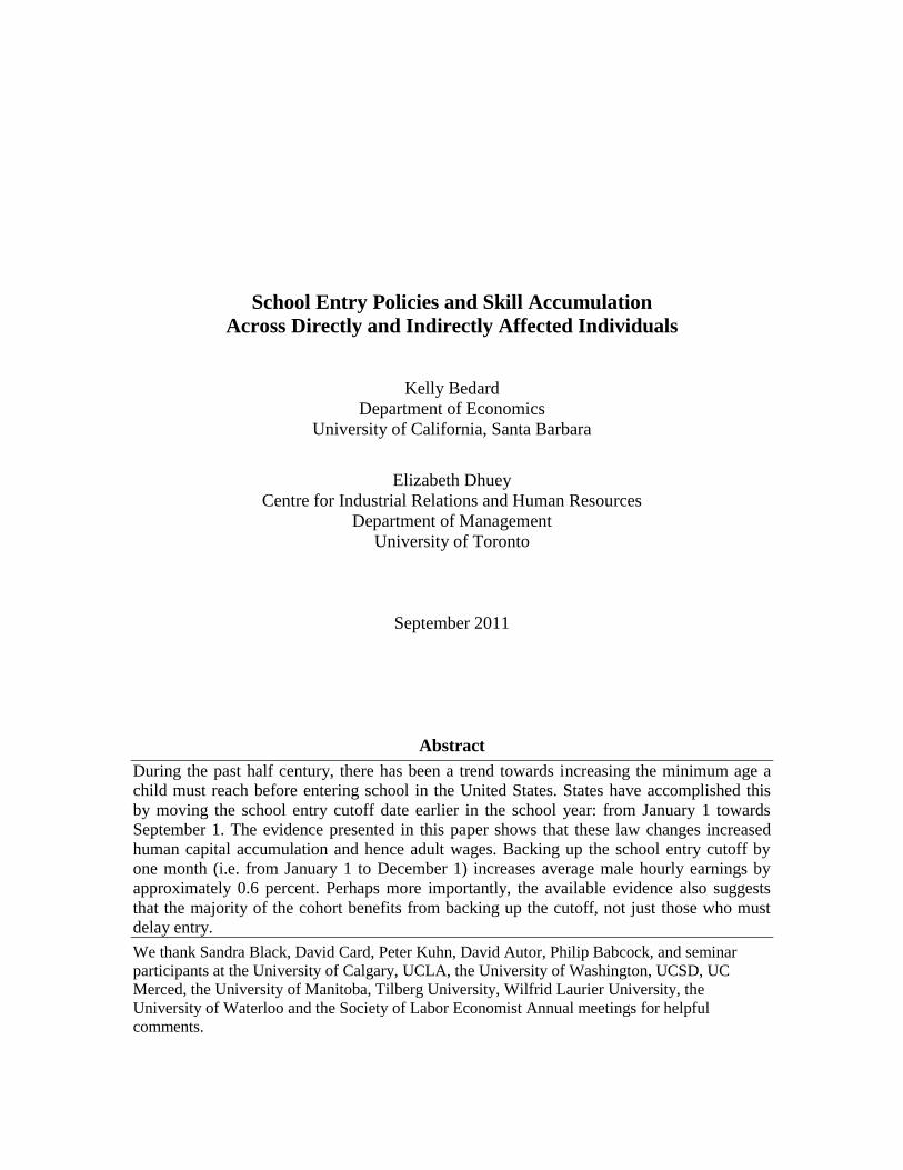
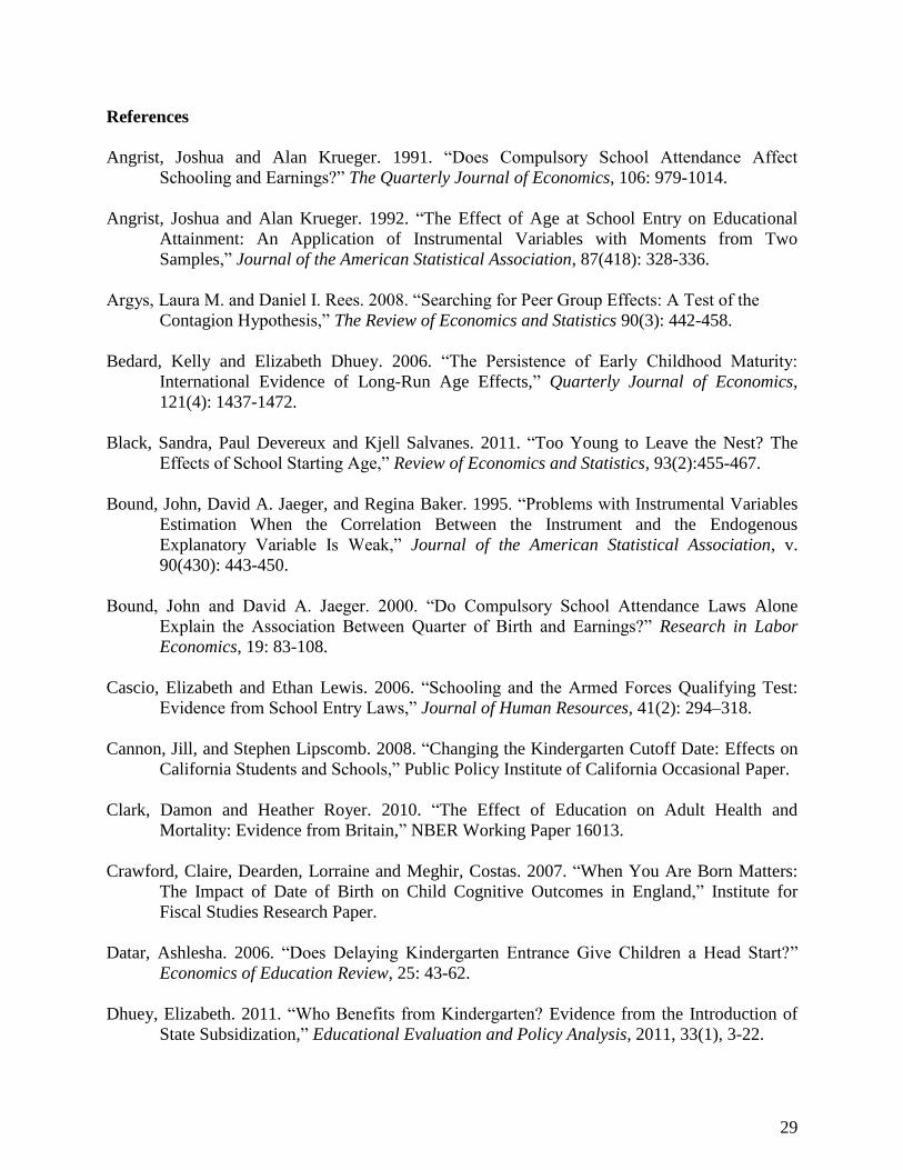
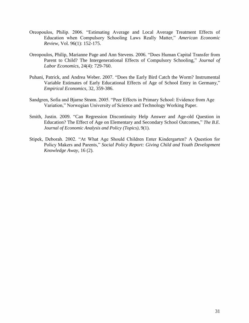
Before probing the estimates further, it is worth pausing to display the results for states

that experience a school entry age policy change graphically. Figures 1 and 2 display the wage

and education data for men and women, respectively. These figures plot the mean residuals

before and after cutoff changes29

from regressions that include only age controls.30

A strong

positive pattern emerges for ln hourly wages for males in Figure 1.1— average ln hourly wages

are higher after the cutoff date changes. However, similar to the results reported in Tables 4 and

5, no other clear pattern emerges for education for either sex or for women‘s ln hourly wages.

28

Appendix Table 5 reports the results for a placebo check of the randomization of the changes in the minimum

school entry age across demographic characteristics and education policy controls. There is little evidence that entry

age law changes are correlated with the available controls. Only one coefficient is statistically significant at the 5%

level—other race. This result reflects the fact that a few have unusually large increases in their Asian population that

occurred roughly during the same period as changes in entry age laws. 29

We plot the residuals for 4-8 years before the first cutoff change and 4-8 years after the last cutoff change. The

long gaps in the figures are necessary because many states slowly changed their cutoff dates over a period of several

years (See Appendix Table 1). 30

Figures 1.1 and 2.1 only include individuals who are not in school, not in prison, work for wages (are not self-

employed) and report positive income.

22

Panel C in Table 5 restricts the sample to full-year/full-time workers defined as reporting

employment of at least 30 usual hours per week, with at least 46 weeks of work, and $2000 in

annual earnings. This sample is included to help shed light on the pattern of female point

estimates reported in the remainder of the Tables 5 and 6. Once we focus on women who are

firmly attached to the labor market, there are few differences between the male and female point

estimates. The lone exception is the last specification, which falls to zero for men. In contrast,

the point estimates for the subsample age 30 or more (Panel D) fall to zero for women but remain

similar to the base specification for men. While this subsample has the benefit of ensuring that

education is largely complete, it also puts more weight on women during child bearing/rearing

years when labor market attachment is often weaker. The difference in male-female labor market

attachment is easily seen by comparing sample sizes at the bottom of the table.

The point estimates for wages naturally lead one to wonder about the impact on labor

force participation. Panel E examines this.31

Whether we measure labor market participation as

being in the labor force, being employed or being full-time/full-year we find that backing up the

school starting age increases male labor market participation, but has no impact on women.

More specifically, measured by in the labor force, the male point estimates range from a 0.11-

0.12 percentage point increases in the in the labor force reports per month that the school starting

age is backed up. As such, the positive male wage effects are not the result of driving men at the

bottom of the earnings distribution out of the labor market. In contrast, there is no discernable

labor force participation effect for women regardless of the definition used. The sample sizes at

the bottom of the table suggest that female selection into and out of the labor market is the most

likely reason for this difference. More specifically, a large fraction of women are choosing to

31

Panel E also includes whether the individual is currently in school as an outcome variable. We find no effect of

the minimum school starting age on this outcome.

23

either stay out of the labor market or only partially participate at different ages and in different

years (likely due to fertility and marriage) in large enough numbers and in heterogeneous enough

ways that it is impossible to detect the small types of effect we are looking for.

While the results reported in Table 5 point to a substantial return to later school entry

dates, they also raise the question of exactly who benefits from the policy change. Does the wage

return largely reflect an increase for those whose school entry is directly affected, or are there

indirect effects for other members of the cohort as well? Our ability to examine this issue is

limited by the relative scarcity of birth date data. However, beginning in 2005 the ACS reports

quarter of birth. The 2005-2007 ACS data can therefore be used to examine, at least crudely, the

impact of cutoff date changes on specific segments of class cohorts. We use the term crude

because quarter of birth does not allow for exact identification of school cutoff for all birth

months.

For the cohorts included in this analysis, only people born between September 1-

December 31 are directly affected by cutoff law changes (see Appendix Table 1). The

aggregation of birthdays to the quarter of birth level in the ACS substantially complicates the

analysis of who is affected. The problem arises because the policy change may affect children

either directly or indirectly, despite their being from the same quarter of birth. For example,

children born in December are directly affected when the cutoff is moved from January 1 to

December 1, whereas children born in October and November are indirectly affected. As the

ACS does not allow us to identify at any level more detailed than quarter of birth, we cannot

separate the directly affected children from the indirectly affected children in this case.

Unfortunately, these types of within quarter changes make up the majority of the cutoff changes

during the sample period. The estimates for both third (July-September) and fourth (October-

24

December) birth quarters are therefore difficult to interpret. This further means that it is

impossible to cleanly estimate the minimum age entry effect for directly affected children.

Given the fact that all cutoff changes during the sample period occur between September

1-December 31, on the surface it therefore appears that the impact of cutoff changes for quarters

one (January-March) and two (April-June) should be easily interpretable since all children in

these groups are indirectly affected. While this is true for quarter two, the quarter one estimates

should be interpreted with care due to possible non-random changes in voluntary school entry.

As the cutoff is backed up from December 31 towards earlier in the fall, it is likely that fewer

first quarter children enter school before they are legally eligible; parents stop enrolling their

children in school early. As such, a small fraction of first quarter children are essentially directly

affected by the policy change. The quarter one estimates cannot therefore be interpreted as

purely indirect. This leaves us with quarter two. We can obtain a lower bound estimate of the

cohort age effect using this sub-group. It is a lower bound because we cannot separate the

positive cohort effect and the negative relative age effect.

Operationally, we modify equation (1) to allow cutoff changes to differentially impact

individuals born in different birth quarters. More specifically, we add indicators for first, second,

and third quarters of birth and interact these indicators with the state of birth specific age at

which the youngest member of the cohort is eligible to enter school. We also interact quarter of

birth with state of birth, region of birth specific cohort indicators, state of birth specific indicators

for years surrounding cutoff changes.

Table 6 reports the impact of the minimum school starting age on ln hourly wages by

birth quarter using the 2005-2007 ACS. For comparative purposes, Panel A reports 1̂ for

equation (1) using only the 2005-2007 ACS. The next four rows (Panel B) report the quarter of

25

birth specific effects of backing up the cutoff by one month (from the quarter of birth interacted

model). For descriptive ease, denote the coefficient on S as 1 and the coefficients on S

interacted with the birth quarter one, two, and three indicators as ,, 32 4 and , respectively for

the quarter of birth interacted model. Row 1 reports 1̂ and its corresponding standard error and

rows 2-4 report the interaction terms ( ,ˆ,ˆ32 4

ˆ and ) and their appropriate standard errors.32

We begin by focusing on men in columns 1-4. To facilitate the presentation of results on

a single page, all columns use the column 3 specification from Tables 4 and 5, our preferred

specification. Column 1 reports the results for ln hourly wages. The point estimates for youngest

legal entry age are positive and statistically significant and the interaction terms for quarters one

and two are small and statistically insignificant. In other words, we cannot reject the null

hypothesis that backing up the cutoff by one month has the same effect on quarters one and two

as it does on four. In contrast, the interaction term for quarter three is always negative and

statistically significant at conventional levels, and we cannot reject the null hypothesis that

041 . The findings for quarter three likely reflect the following factors. First, the majority

of this group becomes the relatively youngest in most cases, which is a negative effect. Second,

similar to quarter four, the point estimate for quarter three is a mixture of direct and indirect

effects. As discussed above, the most interesting result reported in column 1 is the finding that

the point estimate for second quarter men is not statistically distinguishable from that of fourth

quarter men. As the second quarter only includes indirectly affected children, the point estimate

is a mixture of the effect of having an older cohort along with the effect of being relatively

younger in the age distribution. This point estimate is therefore a lower bound for the cohort age

32

For completeness, Appendix Table 6 reports the corresponding results for educational attainment for males and

females, respectively.

26

effect because the relative age effect is negative for this group. This finding is important for at

least two reasons. First, it means that the average point estimates reported in Table 5 reflects both

direct and indirect effects; backing up the school entry cutoff has positive spillover effects that

benefit all or at least most of the cohort. In the absence of these spillovers, the point estimates

reported in Table 5 would be too large. Second, it allows us to separate lost labor market

experience from the school entry age policy effect because the school entry timing of quarter two

children is not altered by the policy change. As such, the concern that we are under-estimating

the impact of the policy change does not apply in this case.

Columns 2-4 run several specification checks. The employment effects reported in

column 2 are smaller and less precise for the 2005-2007 ACS subsample. As a result, we cannot

reject no effect for any birth quarter. In contrast, the wage effect estimates for the full-time/full-

year subsample in column 3 and the age 30 or over subsample in column 4 are similar to the base

specification for men. The one caveat is that the second quarter interaction is too large given the

degree of precision to rule out a zero effect.

The results for the same specifications for women are reported in columns 5-8. As in

Table 5, the only non-zero point estimates are for full-time/full-year women in column 7. In this

case, the point estimate with no quarter of birth interactions (Panel A) is similar to that in Table

5, both in magnitude and in the fact that it is substantially smaller that its male counterpart.

However, the patterns of results reported in the quarter of birth specification (Panel B) differ

somewhat from the male results. In particular, we cannot reject a zero result for either the first or

the second quarter, but we can for the third quarter. We are not entirely sure what to make of the

third quarter results for women. While it is possible this is a real effect, it is also possible that it

27

is an anomaly since the fourth quarter estimates in columns 5 and 8 are much larger, but very

imprecise.

The finding that those indirectly affected benefit from later school entry suggests that

children benefit from having older peers in the classroom. However, very little literature exists

regarding the effect of having older peers. Both Leuven and Rønning (2011) and Sandgren and

Strøm (2005) find that students in Norway benefit from sharing the classroom with older peers.

Leuven and Rønning (2011) conclude that the students in multi-grade classrooms perform better

than students in single-grade classrooms perform and attribute this to students benefiting from

sharing the classroom with older peers. Sandgren and Strøm (2005) examine whether students

with older peers achieve higher achievement levels in math and reading in 4th grade. They find a

positive effect on achievement for male students but not for females. However, Argys and Rees

(2008) find that females with older peers are more likely to use marijuana, alcohol and tobacco

versus females with younger peers but find no effect for males.

While the available data is not ideal, in the sense that we cannot perfectly separate

directly and indirectly affected individuals, Table 6 still delivers a very important finding:

Backing up the cutoff date has an economically significant positive effect for both directly and

indirectly affected individuals.

6. Conclusion

This paper documents the statistically significant and economically important positive earning

effect associated with backing up school cutoff dates. We find that increasing the minimum

school entry age increases wages, but has no measurable effect on educational attainment. This

implies that increases in within grade human capital acquisition are mostly responsible for the

28

estimated wage return. In particular, a one-month increase in the minimum school entry age

increases wages by about 0.6 percent for males. In addition, we report evidence showing that

minimum entry age law changes have an impact on the fraction of the cohort that is indirectly

affected, not just children directly affected by the policy change.

While backing up cutoff dates is not costless—directly affected individuals are forced to

enter elementary school and the labor market a year later—it likely uses fewer public funds than

many other interventions (class size reductions, for example). This policy is also popular in an

era of national testing because students in earlier cutoff states score higher. Despite the positive

rhetoric, the optimal minimum entry cutoff remains unclear. While the estimates reported in this

paper show that there are gains associated with backing up the cutoff from January to September,

they do not tell us whether there would be gains or losses associated with backing it up farther.

The results reported in this paper also suggest that caution is required when interpreting

results from models that use school starting policies to instrument for completed education

because these policies have complex effects. We find no systematic relationship between

changes in school starting age rules and completed education for males or females for any

quarter of birth while at the same time finding adult wages effects. This leads us to interpret the

results as coming through increased human capital accumulation within education categories.

The finding of spillover effects on quarters of birth not directly impacted by policy changes is

also important in this regard because positive human capital effects for these groups do not

reflect changes in the timing of school entry.

29

References

Angrist, Joshua and Alan Krueger. 1991. ―Does Compulsory School Attendance Affect

Schooling and Earnings?‖ The Quarterly Journal of Economics, 106: 979-1014.

Angrist, Joshua and Alan Krueger. 1992. ―The Effect of Age at School Entry on Educational

Attainment: An Application of Instrumental Variables with Moments from Two

Samples,‖ Journal of the American Statistical Association, 87(418): 328-336.

Argys, Laura M. and Daniel I. Rees. 2008. ―Searching for Peer Group Effects: A Test of the

Contagion Hypothesis,‖ The Review of Economics and Statistics 90(3): 442-458.

Bedard, Kelly and Elizabeth Dhuey. 2006. ―The Persistence of Early Childhood Maturity:

International Evidence of Long-Run Age Effects,‖ Quarterly Journal of Economics,

121(4): 1437-1472.

Black, Sandra, Paul Devereux and Kjell Salvanes. 2011. ―Too Young to Leave the Nest? The

Effects of School Starting Age,‖ Review of Economics and Statistics, 93(2):455-467.

Bound, John, David A. Jaeger, and Regina Baker. 1995. ―Problems with Instrumental Variables

Estimation When the Correlation Between the Instrument and the Endogenous

Explanatory Variable Is Weak,‖ Journal of the American Statistical Association, v.

90(430): 443-450.

Bound, John and David A. Jaeger. 2000. ―Do Compulsory School Attendance Laws Alone

Explain the Association Between Quarter of Birth and Earnings?‖ Research in Labor

Economics, 19: 83-108.

Cascio, Elizabeth and Ethan Lewis. 2006. ―Schooling and the Armed Forces Qualifying Test:

Evidence from School Entry Laws,‖ Journal of Human Resources, 41(2): 294–318.

Cannon, Jill, and Stephen Lipscomb. 2008. ―Changing the Kindergarten Cutoff Date: Effects on

California Students and Schools,‖ Public Policy Institute of California Occasional Paper.

Clark, Damon and Heather Royer. 2010. ―The Effect of Education on Adult Health and

Mortality: Evidence from Britain,‖ NBER Working Paper 16013.

Crawford, Claire, Dearden, Lorraine and Meghir, Costas. 2007. ―When You Are Born Matters:

The Impact of Date of Birth on Child Cognitive Outcomes in England,‖ Institute for

Fiscal Studies Research Paper.

Datar, Ashlesha. 2006. ―Does Delaying Kindergarten Entrance Give Children a Head Start?‖

Economics of Education Review, 25: 43-62.

Dhuey, Elizabeth. 2011. ―Who Benefits from Kindergarten? Evidence from the Introduction of

State Subsidization,‖ Educational Evaluation and Policy Analysis, 2011, 33(1), 3-22.

30

Dhuey, Elizabeth and Stephen Lipscomb. 2008. ―What Makes A Leader? Relative Age and High

School Leadership,‖ Economics of Education Review, 27(2): 173-183.

Digest of Educational Statistics. National Center for Education Statistics. U.S. Dept. of Health,

Education, and Welfare, Office of Education.

Dobkin, Carlos and Fernando Ferreira. 2010. ―Do School Entry Laws Affect Educational

Attainment and Labor Market Outcomes,‖ Economics of Education Review, 29(1): 40-54.

Education Research Service. 1975. ―Kindergarten and First Grade Minimum Entrance Age

Policies,‖ ERS Informant.

Elder, Todd and Darren Lubotsky. 2009. ―Kindergarten Entrance Age and Children‘s

Achievement: Impacts of State Policies, Family Background, and Peers,‖ Journal of

Human Resources, 44: 641-683.

Fertig, Michael and Jochen Kluve. 2005. ―The Effect of Age at School Entry on Educational

Attainment in Germany.‖ IZA Discussion Paper Number 1507.

Fredriksson, Peter and Björn Öckert. 2008. ―The Effect of School Starting Age on School and

Labor Market Performance,‖ Stockholm University Working Paper.

Heckman, James, Anne Layne-Farrar and Petra Todd. 1996. ―Does Measured School Quality

Really Matter? An Examination of the Earnings-Quality Relationship,‖ in Burtless, G.

(ed.) Does Money Matter? The Effect of School Resources on Student Achievement and

Success. Brookings, July.

Kawaguchi, Daiji. 2011. ―Actual Age at School Entry, Educational Outcomes, and Earnings,‖

Journal of the Japanese and International Economies, 25(2): 64-80.

Lleras-Muney, Adriana. 2005. ―The Relationship Between Education and Adult Mortality in the

U.S.,‖ Review of Economic Studies, 72(250): 189-221.

Leuven, Edwin and Marte Rønning. 2011. ―Classroom Grade Composition and Pupil

Achievement,‖ École Nationale de la Statistique et de l‘Administration Économique

Working Paper.

McCrary, Justin and Heather Royer. 2011. ―The Effect of Female Education on Fertility and

Infant Health: Evidence from School Entry Policies Using Exact Date of Birth,‖

American Economic Review, 101(1): 158-195.

Mazumder, Bhashkar. 2008. ―Does Education Improve Health: A Reexamination of the

Evidence from Compulsory Schooling Laws,‖ Economic Perspectives, 33(2).

31

Oreopoulos, Philip. 2006. ―Estimating Average and Local Average Treatment Effects of

Education when Compulsory Schooling Laws Really Matter,‖ American Economic

Review, Vol. 96(1): 152-175.

Oreopoulos, Philip, Marianne Page and Ann Stevens. 2006. ―Does Human Capital Transfer from

Parent to Child? The Intergenerational Effects of Compulsory Schooling,‖ Journal of

Labor Economics, 24(4): 729-760.

Puhani, Patrick, and Andrea Weber. 2007. ―Does the Early Bird Catch the Worm? Instrumental

Variable Estimates of Early Educational Effects of Age of School Entry in Germany,‖

Empirical Economics, 32, 359-386.

Sandgren, Sofia and Bjarne Strøm. 2005. ―Peer Effects in Primary School: Evidence from Age

Variation,‖ Norwegian University of Science and Technology Working Paper.

Smith, Justin. 2009. ―Can Regression Discontinuity Help Answer and Age-old Question in

Education? The Effect of Age on Elementary and Secondary School Outcomes,‖ The B.E.

Journal of Economic Analysis and Policy (Topics), 9(1).

Stipek, Deborah. 2002. ―At What Age Should Children Enter Kindergarten? A Question for

Policy Makers and Parents,‖ Social Policy Report: Giving Child and Youth Development

Knowledge Away, 16 (2).

-.1

-.06

-.02

.02

-.1

-.06

-.02

.02

-8 -6 -4 -2 0 2 4 6 8 -8 -6 -4 -2 0 2 4 6 8

1. Ln Hourly Wage 2. % High School Graduate +

3. % Some College + 4. % BA +

Re

sid

ua

l

Years Before/After Policy Change

Figure 1: Pre and Post Entry Age Changes for Males-.

1-.

06

-.02

.02

-.1

-.06

-.02

.02

-8 -6 -4 -2 0 2 4 6 8 -8 -6 -4 -2 0 2 4 6 8

1. Ln Hourly Wage 2. % High School Graduate +

3. % Some College + 4. % BA +

Re

sid

ua

l

Years Before/After Policy Change

Figure 2: Pre and Post Entry Age Changes for Females

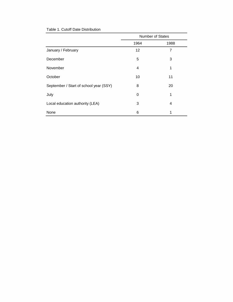
Table 1. Cutoff Date Distribution

1964 1988

January / February 12 7

December 5 3

November 4 1

October 10 11

September / Start of school year (SSY) 8 20

July 0 1

Local education authority (LEA) 3 4

None 6 1

Number of States

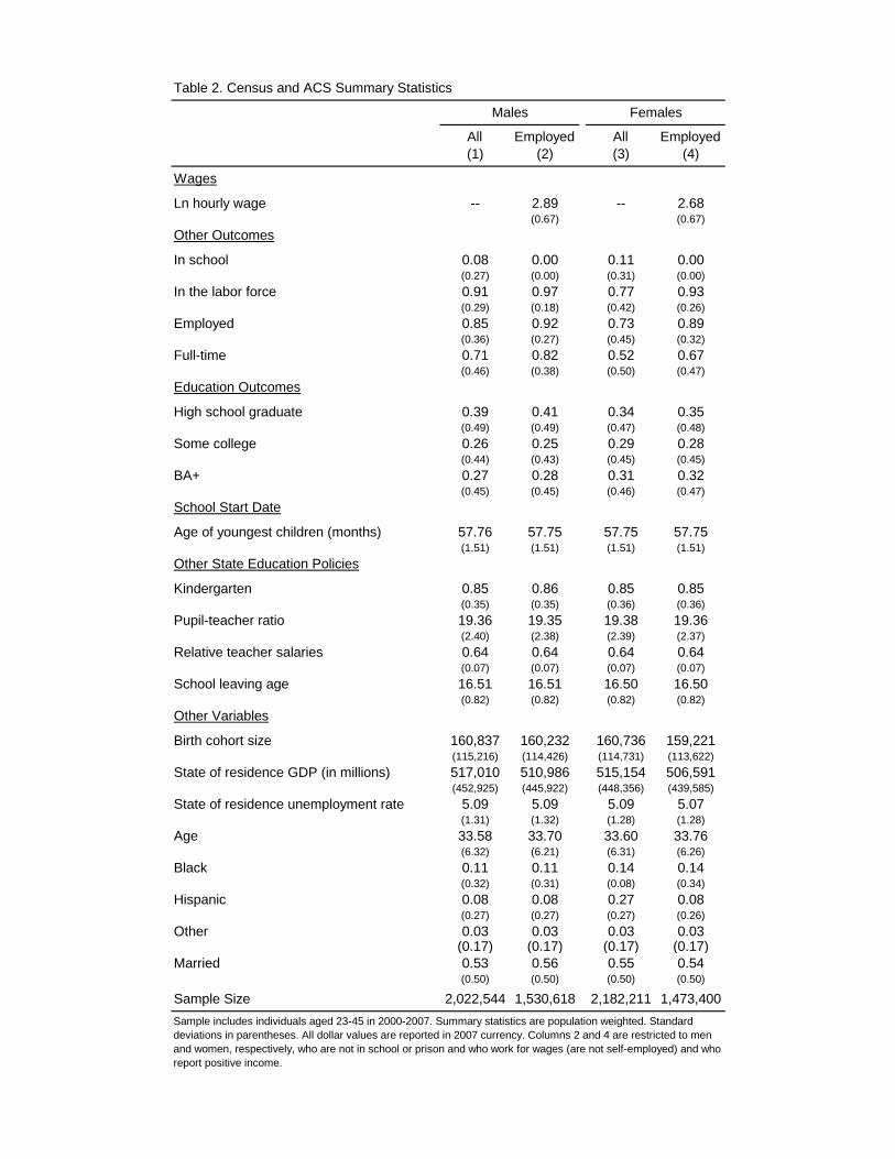
Table 2. Census and ACS Summary Statistics

All Employed All Employed

(1) (2) (3) (4)

Wages

Ln hourly wage -- 2.89 -- 2.68(0.67) (0.67)

Other Outcomes

In school 0.08 0.00 0.11 0.00(0.27) (0.00) (0.31) (0.00)

In the labor force 0.91 0.97 0.77 0.93(0.29) (0.18) (0.42) (0.26)

Employed 0.85 0.92 0.73 0.89(0.36) (0.27) (0.45) (0.32)

Full-time 0.71 0.82 0.52 0.67(0.46) (0.38) (0.50) (0.47)

Education Outcomes

High school graduate 0.39 0.41 0.34 0.35(0.49) (0.49) (0.47) (0.48)

Some college 0.26 0.25 0.29 0.28(0.44) (0.43) (0.45) (0.45)

BA+ 0.27 0.28 0.31 0.32(0.45) (0.45) (0.46) (0.47)

School Start Date

Age of youngest children (months) 57.76 57.75 57.75 57.75(1.51) (1.51) (1.51) (1.51)

Other State Education Policies

Kindergarten 0.85 0.86 0.85 0.85(0.35) (0.35) (0.36) (0.36)

Pupil-teacher ratio 19.36 19.35 19.38 19.36(2.40) (2.38) (2.39) (2.37)

Relative teacher salaries 0.64 0.64 0.64 0.64(0.07) (0.07) (0.07) (0.07)

School leaving age 16.51 16.51 16.50 16.50(0.82) (0.82) (0.82) (0.82)

Other Variables

Birth cohort size 160,837 160,232 160,736 159,221(115,216) (114,426) (114,731) (113,622)

State of residence GDP (in millions) 517,010 510,986 515,154 506,591(452,925) (445,922) (448,356) (439,585)

State of residence unemployment rate 5.09 5.09 5.09 5.07(1.31) (1.32) (1.28) (1.28)

Age 33.58 33.70 33.60 33.76(6.32) (6.21) (6.31) (6.26)

Black 0.11 0.11 0.14 0.14(0.32) (0.31) (0.08) (0.34)

Hispanic 0.08 0.08 0.27 0.08(0.27) (0.27) (0.27) (0.26)

Other 0.03 0.03 0.03 0.03(0.17) (0.17) (0.17) (0.17)

Married 0.53 0.56 0.55 0.54(0.50) (0.50) (0.50) (0.50)

Sample Size 2,022,544 1,530,618 2,182,211 1,473,400

Sample includes individuals aged 23-45 in 2000-2007. Summary statistics are population weighted. Standard

deviations in parentheses. All dollar values are reported in 2007 currency. Columns 2 and 4 are restricted to men

and women, respectively, who are not in school or prison and who work for wages (are not self-employed) and who

report positive income.

Males Females

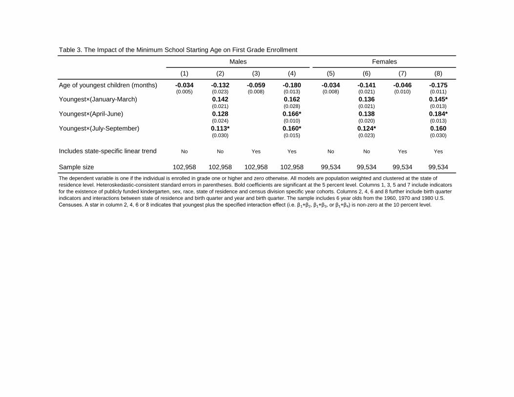
Table 3. The Impact of the Minimum School Starting Age on First Grade Enrollment

(1) (2) (3) (4) (5) (6) (7) (8)

Age of youngest children (months) -0.034 -0.132 -0.059 -0.180 -0.034 -0.141 -0.046 -0.175(0.005) (0.023) (0.008) (0.013) (0.008) (0.021) (0.010) (0.011)

Youngest×(January-March) 0.142 0.162 0.136 0.145*(0.021) (0.028) (0.021) (0.013)

Youngest×(April-June) 0.128 0.166* 0.138 0.184*(0.024) (0.010) (0.020) (0.013)

Youngest×(July-September) 0.113* 0.160* 0.124* 0.160(0.030) (0.015) (0.023) (0.030)

Includes state-specific linear trend No No Yes Yes No No Yes Yes

Sample size 102,958 102,958 102,958 102,958 99,534 99,534 99,534 99,534

Females

The dependent variable is one if the individual is enrolled in grade one or higher and zero otherwise. All models are population weighted and clustered at the state of

residence level. Heteroskedastic-consistent standard errors in parentheses. Bold coefficients are significant at the 5 percent level. Columns 1, 3, 5 and 7 include indicators

for the existence of publicly funded kindergarten, sex, race, state of residence and census division specific year cohorts. Columns 2, 4, 6 and 8 further include birth quarter

indicators and interactions between state of residence and birth quarter and year and birth quarter. The sample includes 6 year olds from the 1960, 1970 and 1980 U.S.

Censuses. A star in column 2, 4, 6 or 8 indicates that youngest plus the specified interaction effect (i.e. β1+β2, β1+β3, or β1+β4) is non-zero at the 10 percent level.

Males

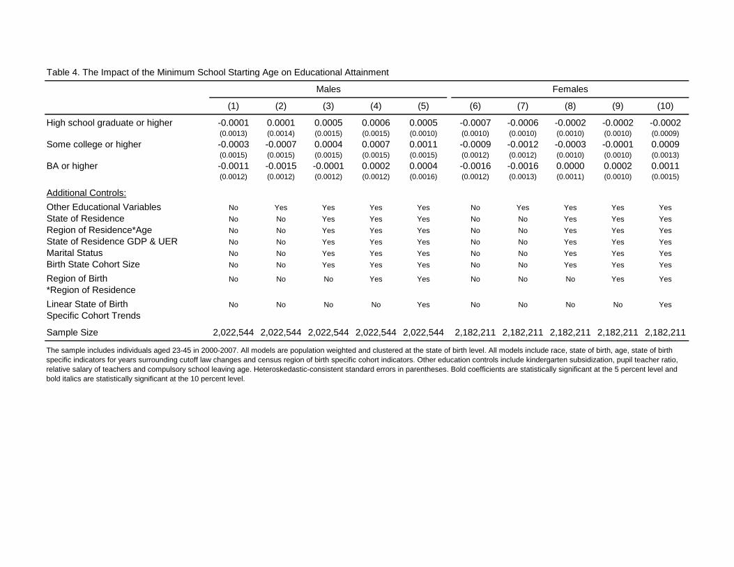
Table 4. The Impact of the Minimum School Starting Age on Educational Attainment

(1) (2) (3) (4) (5) (6) (7) (8) (9) (10)

High school graduate or higher -0.0001 0.0001 0.0005 0.0006 0.0005 -0.0007 -0.0006 -0.0002 -0.0002 -0.0002(0.0013) (0.0014) (0.0015) (0.0015) (0.0010) (0.0010) (0.0010) (0.0010) (0.0010) (0.0009)

Some college or higher -0.0003 -0.0007 0.0004 0.0007 0.0011 -0.0009 -0.0012 -0.0003 -0.0001 0.0009(0.0015) (0.0015) (0.0015) (0.0015) (0.0015) (0.0012) (0.0012) (0.0010) (0.0010) (0.0013)

BA or higher -0.0011 -0.0015 -0.0001 0.0002 0.0004 -0.0016 -0.0016 0.0000 0.0002 0.0011(0.0012) (0.0012) (0.0012) (0.0012) (0.0016) (0.0012) (0.0013) (0.0011) (0.0010) (0.0015)

Additional Controls:

Other Educational Variables No Yes Yes Yes Yes No Yes Yes Yes Yes

State of Residence No No Yes Yes Yes No No Yes Yes Yes

Region of Residence*Age No No Yes Yes Yes No No Yes Yes Yes

State of Residence GDP & UER No No Yes Yes Yes No No Yes Yes Yes

Marital Status No No Yes Yes Yes No No Yes Yes Yes

Birth State Cohort Size No No Yes Yes Yes No No Yes Yes Yes

Region of Birth No No No Yes Yes No No No Yes Yes

*Region of Residence

Linear State of Birth No No No No Yes No No No No Yes

Specific Cohort Trends

Sample Size 2,022,544 2,022,544 2,022,544 2,022,544 2,022,544 2,182,211 2,182,211 2,182,211 2,182,211 2,182,211

Males Females

The sample includes individuals aged 23-45 in 2000-2007. All models are population weighted and clustered at the state of birth level. All models include race, state of birth, age, state of birth

specific indicators for years surrounding cutoff law changes and census region of birth specific cohort indicators. Other education controls include kindergarten subsidization, pupil teacher ratio,

relative salary of teachers and compulsory school leaving age. Heteroskedastic-consistent standard errors in parentheses. Bold coefficients are statistically significant at the 5 percent level and

bold italics are statistically significant at the 10 percent level.

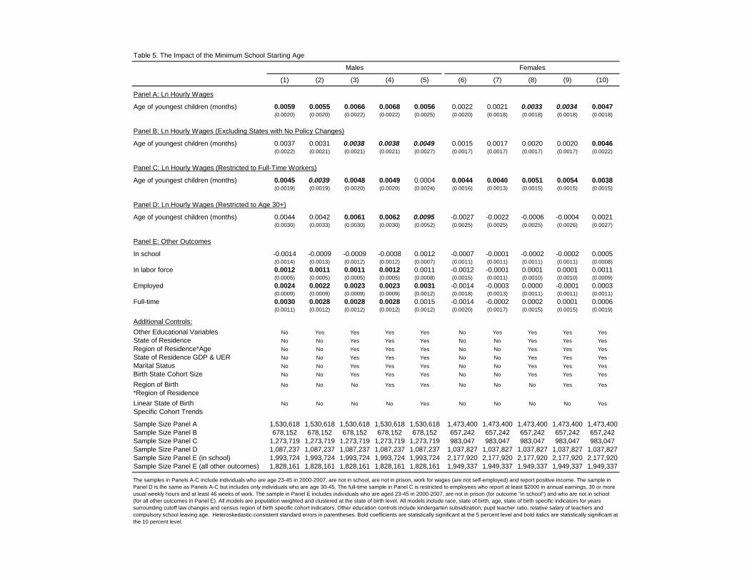
Table 5. The Impact of the Minimum School Starting Age

(1) (2) (3) (4) (5) (6) (7) (8) (9) (10)

Panel A: Ln Hourly Wages

Age of youngest children (months) 0.0059 0.0055 0.0066 0.0068 0.0056 0.0022 0.0021 0.0033 0.0034 0.0047(0.0020) (0.0020) (0.0022) (0.0022) (0.0025) (0.0020) (0.0018) (0.0018) (0.0018) (0.0018)

Panel B: Ln Hourly Wages (Excluding States with No Policy Changes)

Age of youngest children (months) 0.0037 0.0031 0.0038 0.0038 0.0049 0.0015 0.0017 0.0020 0.0020 0.0046(0.0022) (0.0021) (0.0021) (0.0021) (0.0027) (0.0017) (0.0017) (0.0017) (0.0017) (0.0022)

Panel C: Ln Hourly Wages (Restricted to Full-Time Workers)

Age of youngest children (months) 0.0045 0.0039 0.0048 0.0049 0.0004 0.0044 0.0040 0.0051 0.0054 0.0038(0.0019) (0.0019) (0.0020) (0.0020) (0.0024) (0.0016) (0.0013) (0.0015) (0.0015) (0.0015)

Panel D: Ln Hourly Wages (Restricted to Age 30+)

Age of youngest children (months) 0.0044 0.0042 0.0061 0.0062 0.0095 -0.0027 -0.0022 -0.0006 -0.0004 0.0021(0.0030) (0.0033) (0.0030) (0.0030) (0.0052) (0.0025) (0.0025) (0.0025) (0.0026) (0.0027)

Panel E: Other Outcomes

In school -0.0014 -0.0009 -0.0009 -0.0008 0.0012 -0.0007 -0.0001 -0.0002 -0.0002 0.0005(0.0014) (0.0013) (0.0012) (0.0012) (0.0007) (0.0011) (0.0011) (0.0011) (0.0011) (0.0008)

In labor force 0.0012 0.0011 0.0011 0.0012 0.0011 -0.0012 -0.0001 0.0001 0.0001 0.0011(0.0005) (0.0005) (0.0005) (0.0005) (0.0008) (0.0015) (0.0011) (0.0010) (0.0010) (0.0009)

Employed 0.0024 0.0022 0.0023 0.0023 0.0031 -0.0014 -0.0003 0.0000 -0.0001 0.0003(0.0009) (0.0009) (0.0009) (0.0009) (0.0012) (0.0018) (0.0013) (0.0011) (0.0011) (0.0011)

Full-time 0.0030 0.0028 0.0028 0.0028 0.0015 -0.0014 -0.0002 0.0002 0.0001 0.0006(0.0011) (0.0012) (0.0012) (0.0012) (0.0012) (0.0020) (0.0017) (0.0015) (0.0015) (0.0019)

Additional Controls:

Other Educational Variables No Yes Yes Yes Yes No Yes Yes Yes Yes

State of Residence No No Yes Yes Yes No No Yes Yes Yes

Region of Residence*Age No No Yes Yes Yes No No Yes Yes Yes

State of Residence GDP & UER No No Yes Yes Yes No No Yes Yes Yes

Marital Status No No Yes Yes Yes No No Yes Yes Yes

Birth State Cohort Size No No Yes Yes Yes No No Yes Yes Yes

Region of Birth No No No Yes Yes No No No Yes Yes

*Region of Residence

Linear State of Birth No No No No Yes No No No No Yes

Specific Cohort Trends

Sample Size Panel A 1,530,618 1,530,618 1,530,618 1,530,618 1,530,618 1,473,400 1,473,400 1,473,400 1,473,400 1,473,400

Sample Size Panel B 678,152 678,152 678,152 678,152 678,152 657,242 657,242 657,242 657,242 657,242

Sample Size Panel C 1,273,719 1,273,719 1,273,719 1,273,719 1,273,719 983,047 983,047 983,047 983,047 983,047

Sample Size Panel D 1,087,237 1,087,237 1,087,237 1,087,237 1,087,237 1,037,827 1,037,827 1,037,827 1,037,827 1,037,827

Sample Size Panel E (in school) 1,993,724 1,993,724 1,993,724 1,993,724 1,993,724 2,177,920 2,177,920 2,177,920 2,177,920 2,177,920

Sample Size Panel E (all other outcomes) 1,828,161 1,828,161 1,828,161 1,828,161 1,828,161 1,949,337 1,949,337 1,949,337 1,949,337 1,949,337

The samples in Panels A-C include individuals who are age 23-45 in 2000-2007, are not in school, are not in prison, work for wages (are not self-employed) and report positive income. The sample in

Panel D is the same as Panels A-C but includes only individuals who are age 30-45. The full-time sample in Panel C is restricted to employees who report at least $2000 in annual earnings, 30 or more

usual weekly hours and at least 46 weeks of work. The sample in Panel E includes individuals who are aged 23-45 in 2000-2007, are not in prison (for outcome "in school") and who are not in school

(for all other outcomes in Panel E). All models are population weighted and clustered at the state of birth level. All models include race, state of birth, age, state of birth specific indicators for years

surrounding cutoff law changes and census region of birth specific cohort indicators. Other education controls include kindergarten subsidization, pupil teacher ratio, relative salary of teachers and

compulsory school leaving age. Heteroskedastic-consistent standard errors in parentheses. Bold coefficients are statistically significant at the 5 percent level and bold italics are statistically significant at

the 10 percent level.

Males Females

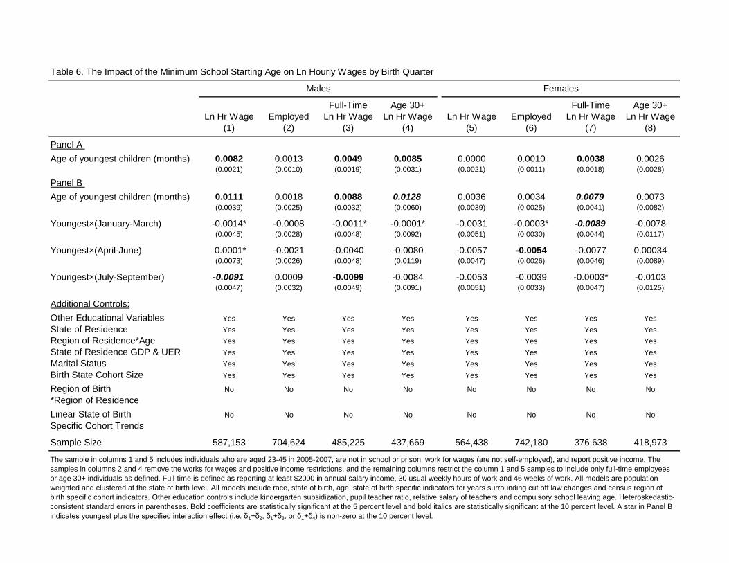
Table 6. The Impact of the Minimum School Starting Age on Ln Hourly Wages by Birth Quarter

Full-Time Age 30+ Full-Time Age 30+

Ln Hr Wage Employed Ln Hr Wage Ln Hr Wage Ln Hr Wage Employed Ln Hr Wage Ln Hr Wage

(1) (2) (3) (4) (5) (6) (7) (8)

Panel A

Age of youngest children (months) 0.0082 0.0013 0.0049 0.0085 0.0000 0.0010 0.0038 0.0026(0.0021) (0.0010) (0.0019) (0.0031) (0.0021) (0.0011) (0.0018) (0.0028)

Panel B

Age of youngest children (months) 0.0111 0.0018 0.0088 0.0128 0.0036 0.0034 0.0079 0.0073(0.0039) (0.0025) (0.0032) (0.0060) (0.0039) (0.0025) (0.0041) (0.0082)

Youngest×(January-March) -0.0014* -0.0008 -0.0011* -0.0001* -0.0031 -0.0003* -0.0089 -0.0078(0.0045) (0.0028) (0.0048) (0.0092) (0.0051) (0.0030) (0.0044) (0.0117)

Youngest×(April-June) 0.0001* -0.0021 -0.0040 -0.0080 -0.0057 -0.0054 -0.0077 0.00034(0.0073) (0.0026) (0.0048) (0.0119) (0.0047) (0.0026) (0.0046) (0.0089)

Youngest×(July-September) -0.0091 0.0009 -0.0099 -0.0084 -0.0053 -0.0039 -0.0003* -0.0103(0.0047) (0.0032) (0.0049) (0.0091) (0.0051) (0.0033) (0.0047) (0.0125)

Additional Controls:

Other Educational Variables Yes Yes Yes Yes Yes Yes Yes Yes

State of Residence Yes Yes Yes Yes Yes Yes Yes Yes

Region of Residence*Age Yes Yes Yes Yes Yes Yes Yes Yes

State of Residence GDP & UER Yes Yes Yes Yes Yes Yes Yes Yes

Marital Status Yes Yes Yes Yes Yes Yes Yes Yes

Birth State Cohort Size Yes Yes Yes Yes Yes Yes Yes Yes

Region of Birth No No No No No No No No

*Region of Residence

Linear State of Birth No No No No No No No No

Specific Cohort Trends

Sample Size 587,153 704,624 485,225 437,669 564,438 742,180 376,638 418,973

Males Females

The sample in columns 1 and 5 includes individuals who are aged 23-45 in 2005-2007, are not in school or prison, work for wages (are not self-employed), and report positive income. The

samples in columns 2 and 4 remove the works for wages and positive income restrictions, and the remaining columns restrict the column 1 and 5 samples to include only full-time employees

or age 30+ individuals as defined. Full-time is defined as reporting at least $2000 in annual salary income, 30 usual weekly hours of work and 46 weeks of work. All models are population

weighted and clustered at the state of birth level. All models include race, state of birth, age, state of birth specific indicators for years surrounding cut off law changes and census region of

birth specific cohort indicators. Other education controls include kindergarten subsidization, pupil teacher ratio, relative salary of teachers and compulsory school leaving age. Heteroskedastic-

consistent standard errors in parentheses. Bold coefficients are statistically significant at the 5 percent level and bold italics are statistically significant at the 10 percent level. A star in Panel B

indicates youngest plus the specified interaction effect (i.e. δ1+δ2, δ1+δ3, or δ1+δ4) is non-zero at the 10 percent level.

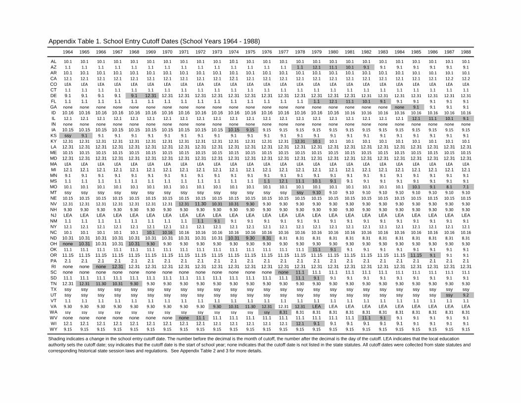
Appendix Table 1. School Entry Cutoff Dates (School Years 1964 - 1988)

1964 1965 1966 1967 1968 1969 1970 1971 1972 1973 1974 1975 1976 1977 1978 1979 1980 1981 1982 1983 1984 1985 1986 1987 1988

AL 10.1 10.1 10.1 10.1 10.1 10.1 10.1 10.1 10.1 10.1 10.1 10.1 10.1 10.1 10.1 10.1 10.1 10.1 10.1 10.1 10.1 10.1 10.1 10.1 10.1AZ 1.1 1.1 1.1 1.1 1.1 1.1 1.1 1.1 1.1 1.1 1.1 1.1 1.1 1.1 1.1 12.1 11.1 10.1 9.1 9.1 9.1 9.1 9.1 9.1 9.1AR 10.1 10.1 10.1 10.1 10.1 10.1 10.1 10.1 10.1 10.1 10.1 10.1 10.1 10.1 10.1 10.1 10.1 10.1 10.1 10.1 10.1 10.1 10.1 10.1 10.1CA 12.1 12.1 12.1 12.1 12.1 12.1 12.1 12.1 12.1 12.1 12.1 12.1 12.1 12.1 12.1 12.1 12.1 12.1 12.1 12.1 12.1 12.1 12.1 12.2 12.2CO LEA LEA LEA LEA LEA LEA LEA LEA LEA LEA LEA LEA LEA LEA LEA LEA LEA LEA LEA LEA LEA LEA LEA LEA LEACT 1.1 1.1 1.1 1.1 1.1 1.1 1.1 1.1 1.1 1.1 1.1 1.1 1.1 1.1 1.1 1.1 1.1 1.1 1.1 1.1 1.1 1.1 1.1 1.1 1.1DE 9.1 9.1 9.1 9.1 9.1 12.31 12.31 12.31 12.31 12.31 12.31 12.31 12.31 12.31 12.31 12.31 12.31 12.31 12.31 12.31 12.31 12.31 12.31 12.31 12.31FL 1.1 1.1 1.1 1.1 1.1 1.1 1.1 1.1 1.1 1.1 1.1 1.1 1.1 1.1 1.1 1.1 12.1 11.1 10.1 9.1 9.1 9.1 9.1 9.1 9.1GA none none none none none none none none none none none none none none none none none none none none none 9.1 9.1 9.1 9.1ID 10.16 10.16 10.16 10.16 10.16 10.16 10.16 10.16 10.16 10.16 10.16 10.16 10.16 10.16 10.16 10.16 10.16 10.16 10.16 10.16 10.16 10.16 10.16 10.16 10.16IL 12.1 12.1 12.1 12.1 12.1 12.1 12.1 12.1 12.1 12.1 12.1 12.1 12.1 12.1 12.1 12.1 12.1 12.1 12.1 12.1 12.1 12.1 11.1 10.1 9.1IN none none none none none none none none none none none none none none none none none none none none none none none none noneIA 10.15 10.15 10.15 10.15 10.15 10.15 10.15 10.15 10.15 10.15 10.15 9.15 9.15 9.15 9.15 9.15 9.15 9.15 9.15 9.15 9.15 9.15 9.15 9.15 9.15KS ssy 9.1 9.1 9.1 9.1 9.1 9.1 9.1 9.1 9.1 9.1 9.1 9.1 9.1 9.1 9.1 9.1 9.1 9.1 9.1 9.1 9.1 9.1 9.1 9.1KY 12.31 12.31 12.31 12.31 12.31 12.31 12.31 12.31 12.31 12.31 12.31 12.31 12.31 12.31 12.31 10.1 10.1 10.1 10.1 10.1 10.1 10.1 10.1 10.1 10.1LA 12.31 12.31 12.31 12.31 12.31 12.31 12.31 12.31 12.31 12.31 12.31 12.31 12.31 12.31 12.31 12.31 12.31 12.31 12.31 12.31 12.31 12.31 12.31 12.31 12.31

ME 10.15 10.15 10.15 10.15 10.15 10.15 10.15 10.15 10.15 10.15 10.15 10.15 10.15 10.15 10.15 10.15 10.15 10.15 10.15 10.15 10.15 10.15 10.15 10.15 10.15MD 12.31 12.31 12.31 12.31 12.31 12.31 12.31 12.31 12.31 12.31 12.31 12.31 12.31 12.31 12.31 12.31 12.31 12.31 12.31 12.31 12.31 12.31 12.31 12.31 12.31

MA LEA LEA LEA LEA LEA LEA LEA LEA LEA LEA LEA LEA LEA LEA LEA LEA LEA LEA LEA LEA LEA LEA LEA LEA LEAMI 12.1 12.1 12.1 12.1 12.1 12.1 12.1 12.1 12.1 12.1 12.1 12.1 12.1 12.1 12.1 12.1 12.1 12.1 12.1 12.1 12.1 12.1 12.1 12.1 12.1

MN 9.1 9.1 9.1 9.1 9.1 9.1 9.1 9.1 9.1 9.1 9.1 9.1 9.1 9.1 9.1 9.1 9.1 9.1 9.1 9.1 9.1 9.1 9.1 9.1 9.1MS 1.1 1.1 1.1 1.1 1.1 1.1 1.1 1.1 1.1 1.1 1.1 1.1 1.1 12.1 11.1 10.1 9.1 9.1 9.1 9.1 9.1 9.1 9.1 9.1 9.1MO 10.1 10.1 10.1 10.1 10.1 10.1 10.1 10.1 10.1 10.1 10.1 10.1 10.1 10.1 10.1 10.1 10.1 10.1 10.1 10.1 10.1 10.1 9.1 8.1 7.1MT ssy ssy ssy ssy ssy ssy ssy ssy ssy ssy ssy ssy ssy ssy ssy 9.10 9.10 9.10 9.10 9.10 9.10 9.10 9.10 9.10 9.10NE 10.15 10.15 10.15 10.15 10.15 10.15 10.15 10.15 10.15 10.15 10.15 10.15 10.15 10.15 10.15 10.15 10.15 10.15 10.15 10.15 10.15 10.15 10.15 10.15 10.15NV 12.31 12.31 12.31 12.31 12.31 12.31 12.31 12.31 11.30 10.31 10.31 9.30 9.30 9.30 9.30 9.30 9.30 9.30 9.30 9.30 9.30 9.30 9.30 9.30 9.30NH 9.30 9.30 9.30 9.30 9.30 9.30 9.30 9.30 9.30 9.30 9.30 9.30 9.30 9.30 9.30 9.30 9.30 9.30 9.30 9.30 9.30 9.30 9.30 9.30 9.30NJ LEA LEA LEA LEA LEA LEA LEA LEA LEA LEA LEA LEA LEA LEA LEA LEA LEA LEA LEA LEA LEA LEA LEA LEA LEA

NM 1.1 1.1 1.1 1.1 1.1 1.1 1.1 1.1 1.1 9.1 9.1 9.1 9.1 9.1 9.1 9.1 9.1 9.1 9.1 9.1 9.1 9.1 9.1 9.1 9.1NY 12.1 12.1 12.1 12.1 12.1 12.1 12.1 12.1 12.1 12.1 12.1 12.1 12.1 12.1 12.1 12.1 12.1 12.1 12.1 12.1 12.1 12.1 12.1 12.1 12.1NC 10.1 10.1 10.1 10.1 10.1 10.1 10.16 10.16 10.16 10.16 10.16 10.16 10.16 10.16 10.16 10.16 10.16 10.16 10.16 10.16 10.16 10.16 10.16 10.16 10.16ND 10.31 10.31 10.31 10.31 10.31 10.31 10.31 10.31 10.31 10.31 10.31 9.30 8.31 8.31 8.31 8.31 8.31 8.31 8.31 8.31 8.31 8.31 8.31 8.31 8.31OH none 10.31 10.31 10.31 10.31 9.30 9.30 9.30 9.30 9.30 9.30 9.30 9.30 9.30 9.30 9.30 9.30 9.30 9.30 9.30 9.30 9.30 9.30 9.30 9.30OK 11.1 11.1 11.1 11.1 11.1 11.1 11.1 11.1 11.1 11.1 11.1 11.1 11.1 11.1 11.1 11.1 9.1 9.1 9.1 9.1 9.1 9.1 9.1 9.1 9.1OR 11.15 11.15 11.15 11.15 11.15 11.15 11.15 11.15 11.15 11.15 11.15 11.15 11.15 11.15 11.15 11.15 11.15 11.15 11.15 11.15 11.15 11.15 9.1 9.1 9.1PA 2.1 2.1 2.1 2.1 2.1 2.1 2.1 2.1 2.1 2.1 2.1 2.1 2.1 2.1 2.1 2.1 2.1 2.1 2.1 2.1 2.1 2.1 2.1 2.1 2.1

RI none none none 12.31 12.31 12.31 12.31 12.31 12.31 12.31 12.31 12.31 12.31 12.31 12.31 12.31 12.31 12.31 12.31 12.31 12.31 12.31 12.31 12.31 12.31

SC none none none none none none none none none none none none none none 11.1 11.1 11.1 11.1 11.1 11.1 11.1 11.1 11.1 11.1 11.1SD 11.1 11.1 11.1 11.1 11.1 11.1 11.1 11.1 11.1 11.1 11.1 11.1 11.1 11.1 11.1 9.1 9.1 9.1 9.1 9.1 9.1 9.1 9.1 9.1 9.1TN 12.31 12.31 11.30 10.31 9.30 9.30 9.30 9.30 9.30 9.30 9.30 9.30 9.30 9.30 9.30 9.30 9.30 9.30 9.30 9.30 9.30 9.30 9.30 9.30 9.30TX ssy ssy ssy ssy ssy ssy ssy ssy ssy ssy ssy ssy ssy ssy ssy ssy ssy ssy ssy ssy ssy ssy ssy ssy ssy

UT ssy ssy ssy ssy ssy ssy ssy ssy ssy ssy ssy ssy ssy ssy ssy ssy ssy ssy ssy ssy ssy ssy ssy ssy 9.2VT 1.1 1.1 1.1 1.1 1.1 1.1 1.1 1.1 1.1 1.1 1.1 1.1 1.1 1.1 1.1 1.1 1.1 1.1 1.1 1.1 1.1 1.1 1.1 1.1 1.1VA 9.30 9.30 9.30 9.30 9.30 9.30 9.30 9.30 9.30 9.30 10.31 11.30 12.31 12.31 12.31 LEA LEA LEA LEA LEA LEA LEA LEA LEA LEA

WA ssy ssy ssy ssy ssy ssy ssy ssy ssy ssy ssy ssy ssy 8.31 8.31 8.31 8.31 8.31 8.31 8.31 8.31 8.31 8.31 8.31 8.31WV none none none none none none none none 11.1 11.1 11.1 11.1 11.1 11.1 11.1 11.1 11.1 11.1 11.1 9.1 9.1 9.1 9.1 9.1 9.1WI 12.1 12.1 12.1 12.1 12.1 12.1 12.1 12.1 12.1 12.1 12.1 12.1 12.1 12.1 12.1 9.1 9.1 9.1 9.1 9.1 9.1 9.1 9.1 9.1 9.1WY 9.15 9.15 9.15 9.15 9.15 9.15 9.15 9.15 9.15 9.15 9.15 9.15 9.15 9.15 9.15 9.15 9.15 9.15 9.15 9.15 9.15 9.15 9.15 9.15 9.15

Shading indicates a change in the school entry cutoff date. The number before the decimal is the month of cutoff, the number after the decimal is the day of the cutoff. LEA indicates that the local education

authority sets the cutoff date; ssy indicates that the cutoff date is the start of school year; none indicates that the cutoff date is not listed in the state statutes. All cutoff dates were collected from state statutes and

corresponding historical state session laws and regulations. See Appendix Table 2 and 3 for more details.

Appendix Table 2. State Statutes Regarding School Entry

State Statute AL ST § 16-28-4

AZ ST § 15-821

AR ST § 6-18-207

CA EDUC § 48000

CO ST § 22-32-119

CT ST § 10-15c

DE ST TI 14 § 2702

FL ST § 232.01; ST § 1003.21; ST § 232.04

GA ST § 20-2-150

ID ST § 33-201

IL ST SCH 105 § 5/10-20.12

IN ST § 20-8.1-3-17

IA ST § 282.3

KS ST § 72-1107(c)

KY ST § 158.030

LA R.S. 17:151.3 and 17:222

ME ST T. 20-A § 5201

MD EDUC § 7-101 & § 7-301 & COMAR 13A.08.01.02

MA ST § 76-1

MI ST 380.1147

MN ST § 120A.20

MS ST § 37-15-91

MO ST 160.051

MT ST 20-7-117

NE ST § 79-214

NV ST 392.040

NH ST § 193:1

NJ ST 18A:44-2

NM ST § 22-13-3

NY EDUC § 1712 § 3202

NC ST § 115C-364)

ND ST 15.1-06-01

OH ST § 3321.01

OK ST T. 70 § 1-114

OR ST § 336.092

PA ST 24 PS. § 5-503, §13-1304

RI ST § 16-2-27

SC ST § 59-63-20

SD ST § 13-28-2

TN ST § 49-6-201

TX EDUC § 29.151

UT ST § 53A-3-402

VT ST T. 16 § 1073

VA ST § 22.1-199 & 22-218.1

WA ADC 180-39-010

WV ST § 18-5-18

WI ST 118.14

WY ST § 21-4-302

Cutoff date changes in Appendix 1 were compiled from the state statutes

listed above along with information collected from corresponding historical

state session laws and regulations relating to the statute.

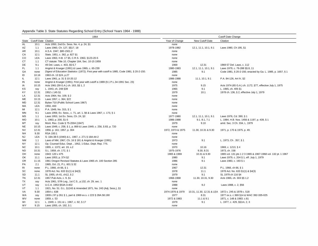
Appendix Table 3. State Statutes Regarding School Entry (School Years 1964 - 1988)

State Cutoff Date Citation Year of Change New Cutoff Date Citation

AL 10.1 Acts 1950, 2nd Ex. Sess. No. 4, p. 24, §1 none

AZ 1.1 Laws 1960, Ch. 127, §§17, 18 1978-1982 12.1, 11.1, 10.1, 9.1 Laws 1980, Ch 195, §1

AR 10.1 A.S.A. 1947, §80-1501.2 none

CA 12.1 Stats. 1951, c. 362, p. 827 §1 none

CO LEA Laws 1963, H.B. 17 §5, C.R.S. 1963, §123-20-5 none

CT 1.1 CT statute: Title 10, Chapter 164, Sec. 10-15 1959 none

DE 9.1 49 Del. Laws, c. 403, §§ 6,7 1969 12.31 1969 57 Del. Laws, c. 112

FL 1.1 Angrist & Krueger (1991) & Laws 1965, c. 65-239 1980-1983 12.1, 11.1, 10.1, 9.1 Laws 1979, c. 79-288 §§ 8, 11

GA none Digest of Education Statistics (1972). First year with cutoff is 1985, Code 1981, § 20-2-150. 1985 9.1 Code 1981, § 20-2-150, enacted by Ga. L. 1985, p. 1657, § 1

ID 10.16 1963 ch. 13 §24, p.27 none

IL 12.1 Laws 1961, p. 31 § 10-20.12 1986-1988 11.1, 10.1, 9.1 P.A. 84-126, Art IV, §2

IN none Angrist & Krueger (1991). First year with cutoff is 1989 (9.1 P.L.34-1991 Sec. 23) none

IA 10.15 Acts 1961 (59 G.A.) ch. 163, §§ 1, 2 1975 9.15 Acts 1974 (65 G.A.) ch. 1172, §77, effective July 1, 1975

KS ssy L. 1943, ch. 248 §39 1965 9.1 L. 1965, ch. 405 §1

KY 12.31 1952 c 145 §1 1979 10.1 1978 ch. 136, § 2, effective July 1, 1979

LA 12.31 Acts 1964, No. 109, § 2 none

ME 10.15 Laws 1957, c. 364, §22 none

MD 12.31 Bylaw 710 (Public School Laws 1967) none

MA LEA 1950, 400 none

MI 12.1 P.A. 1949, No. 315, § 1 none

MN 9.1 Laws 1959, Ex. Sess., c. 71, art. 1, §6 & Laws 1967, c. 173, § 1 none

MS 1.1 Laws 1953, 1st Ex. Sess, Ch. 24, §3 1977-1980 12.1, 11.1, 10.1, 9.1 Laws 1976, Cd. 390, § 1

MO 10.1 L. 1963, p. 200, §1-5 1986-1988 9.1. 8.1, 7.1 L. 1984, H.B. Nos. 1456 & 1197, p. 439, § 1

MT ssy Mont. Rev. Code § 75-2004 (1947) 1979 9.10 amd. Sec. 3 Ch. 334, L. 1979

NE 10.15 Laws 1949, c. 258, § 1, p. 869 & Laws 1949, c. 256, § 83, p. 720 none

NV 12.31 1956, p. 161; 1957, p. 304 1972, 1973 & 1975 11.30, 10.31 & 9.30 1971, p. 170 & 1975, p. 49.

NH 9.30 RSA 193:1 none

NJ LEA S: 18A:38-5 (1940) & L. 1967, c. 271 § 18A:44-2 none

NM 1.1 Laws of NM, 1967, Ch. 16 § 181 & Angrist & Krueger (1991) 1973 9.1 L. 1973, Ch . 357, § 1

NY 12.1 Op. Counsel Educ. Dept. , 1952, 1 Educ. Dept. Rep. 775. none

NC 10.1 1955, c. 1372, art. 19, s.2 1970 10.16 1969, c. 1213, § 4

ND 10.31 S.L. 1959, ch. 172, § 1 1975-1976 9.30, 8.31 1973, ch. 158

OH none 1943: 120 v 475 1965 & 1969 10.31 & 9.30 1965 vol. 131 pts 1 2 3 1965 & 1967-1968 vol. 132 pt. 1 1967

OK 11.1 Laws 1953, p. 374 §2 1980 9.1 Laws 1979, c. 204 § 1, eff. July 1, 1979

OR 11.15 1961 Oregon Revised Statutes & Laws 1965 ch. 100 Section 285 1986 9.1 Laws 1983, c. 193 § 1

PA 2.1 1965, Oct. 21, P.L. 601 § 32 none

RI none P.L. 1966, ch 66, § 1 1967 12.31 P.L. 1966, ch 66, § 1

SC none 1978 Act. No. 633 §1(1) & §4(3) 1978 11.1 1978 Act. No. 633 §1(1) & §4(3)

SD 11.1 SL 1955, ch 41, ch12, § 2 1979 9.1 SL 1979 ch 116 §4

TN 12.31 1957 Pub Acts, c. 9, §1 1966-1968 11.30, 10.31, 9.30 Acts 1965, ch. 303 §§ 1,2

TX ssy Acts 1961, 57th Leg., 1st C.S., p.132, ch. 29, sec. 1 none

UT ssy U.C.A. 1953 §53A-3-402 1988 9.2 Laws 1988, c. 2, §56

VT 1.1 1921, No. 51. G.L. §1243 & Amended 1971, No. 243 (Adj. Sess,), §1 none

VA 9.30 1954 c. 638 1974-1976 & 1979 10.31, 11.30, 12.31 & LEA 1972 c. 245 & 1978 c. 518

WA ssy 1909 c 97 p 261 § 1, part & 1969 ex.s. c 223 § 28A.58.190 1977 8.31 1977 ex.s. c 369 §14 & WAC 392-335-025

WV none 1959, c. 53 1972 & 1983 11.1 & 9.1 1971, c. 148 & 1983. c.61

WI 12.1 L. 1949, c. 151 & L. 1967, c. 92, § 17 1979 9.1 L. 1977, c. 429, §§1m, 2, 3

WY 9.15 Laws 1955, ch. 192, § 1 none

1964 Cutoff Date Change

Appendix Table 4. The Impact of the Minimum School Starting Age on First Grade Enrollment

(1) (2) (3) (4)

Age of youngest children (months) -0.0585 -0.1323 -0.0469 -0.1417(0.0080) (0.0235) (0.0110) (0.0213)

Youngest×(January-March) 0.1411 0.1363(0.0204) (0.0204)

Youngest×(April-June) 0.1287 0.1386(0.0243) (0.0204)

Youngest×(July-September) 0.1134* 0.1240*(0.0311) (0.0236)

Black interactions

Age of youngest children * Black -0.0030* 0.0009* 0.0013* 0.0027*(0.0044) (0.0053) (0.0062) (0.0050)

Youngest×(January-March) * Black 0.0005 0.0011(0.0003) (0.0003)

Youngest×(April-June) * Black -0.0023 -0.0018(0.0003) (0.0002)

Youngest×(July-September) * Black -0.0023* -0.0015*(0.0003) (0.0002)

Hispanic interactions

Age of youngest children * Hispanic 0.0003* 0.0011* -0.0001* 0.0002*(0.0001) (0.0003) (0.0002) (0.0004)

Youngest×(January-March) * Hispanic 0.0002 0.0005(0.0004) (0.0003)

Youngest×(April-June) * Hispanic -0.0016 -0.0012(0.0005) (0.0004)

Youngest×(July-September) * Hispanic -0.0012* -0.0012*(0.0004) (0.0004)

Other race interactions

Age of youngest children * Other race 0.0050* 0.0082* 0.0061* 0.0104*(0.0101) (0.0116) (0.0064) (0.0049)

Youngest×(January-March) * Other race -0.0005 -0.0006(0.0005) (0.0004)

Youngest×(April-June) * Other race -0.0024 -0.0014(0.0004) (0.0004)

Youngest×(July-September) * Other race -0.0018 -0.0019(0.0004) (0.0005)

Sample size 102,958 102,958 99,534 99,534

Males Females

The dependent variable is one if the individual is enrolled in grade one or higher and zero otherwise. All models are

population weighted and clustered at the state of residence level. Heteroskedastic-consistent standard errors in

parentheses. Bold coefficients are significant at the 5 percent level. Columns 1 and 3 include indicators for the existence

of publicly funded kindergarten, sex, race, state of residence and census division specific year cohorts. Columns 2 and 4

further include birth quarter indicators and interactions between state of residence and birth quarter and year and birth

quarter. The sample includes 6 year olds from the 1960, 1970 and 1980 U.S. Censuses. A star indicates that youngest

plus the specified interaction effects are non-zero at the 10 percent level.

Appendix Table 5. Randomization Across Background Demographics and Education Policy Controls

Female -0.0005(0.0006)

Black -0.0014(0.0013)

Hispanic -0.0041(0.0027)

Other race -0.0019(0.0009)

Kindergarten subsidization 0.0149(0.0262)

Pupil teacher ratio -0.0842(0.0881)

Relative salary of teachers 0.0035(0.0020)

Compulsory school leaving age -0.0076(0.0606)

Sample Size 4,204,755

The sample includes males and females aged 23-45 in 2000-2007. All models are population weighted and clustered at the state

of birth level. All models include state of birth, age, state of birth specific indicators for years surrounding cutoff law changes and

census region of birth specific cohort indicators. Heteroskedastic-consistent standard errors in parentheses. Bold coefficients are

statistically significant at the 5 percent level and bold italics are statistically significant at the 10 percent level.

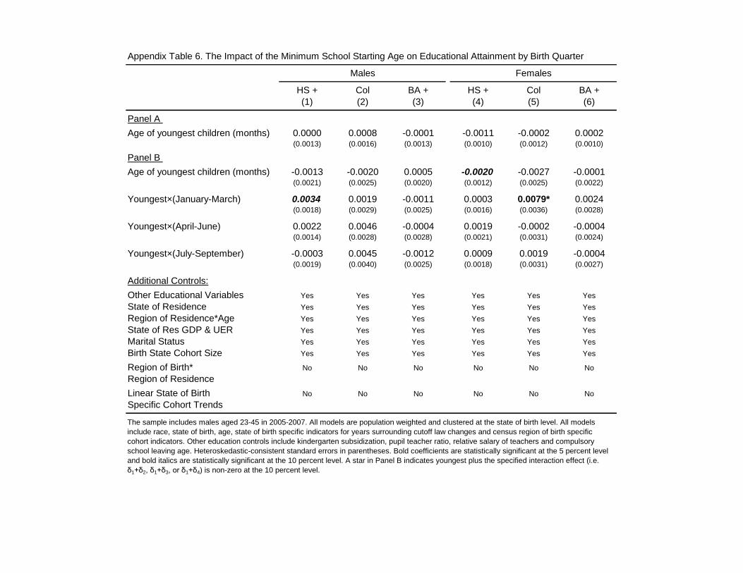
Appendix Table 6. The Impact of the Minimum School Starting Age on Educational Attainment by Birth Quarter

Males Females

HS + Col BA + HS + Col BA +

(1) (2) (3) (4) (5) (6)

Panel A

Age of youngest children (months) 0.0000 0.0008 -0.0001 -0.0011 -0.0002 0.0002(0.0013) (0.0016) (0.0013) (0.0010) (0.0012) (0.0010)

Panel B

Age of youngest children (months) -0.0013 -0.0020 0.0005 -0.0020 -0.0027 -0.0001(0.0021) (0.0025) (0.0020) (0.0012) (0.0025) (0.0022)

Youngest×(January-March) 0.0034 0.0019 -0.0011 0.0003 0.0079* 0.0024(0.0018) (0.0029) (0.0025) (0.0016) (0.0036) (0.0028)

Youngest×(April-June) 0.0022 0.0046 -0.0004 0.0019 -0.0002 -0.0004(0.0014) (0.0028) (0.0028) (0.0021) (0.0031) (0.0024)

Youngest×(July-September) -0.0003 0.0045 -0.0012 0.0009 0.0019 -0.0004(0.0019) (0.0040) (0.0025) (0.0018) (0.0031) (0.0027)

Additional Controls:

Other Educational Variables Yes Yes Yes Yes Yes Yes

State of Residence Yes Yes Yes Yes Yes Yes

Region of Residence*Age Yes Yes Yes Yes Yes Yes

State of Res GDP & UER Yes Yes Yes Yes Yes Yes

Marital Status Yes Yes Yes Yes Yes Yes

Birth State Cohort Size Yes Yes Yes Yes Yes Yes

Region of Birth* No No No No No No

Region of Residence

Linear State of Birth No No No No No No

Specific Cohort Trends

The sample includes males aged 23-45 in 2005-2007. All models are population weighted and clustered at the state of birth level. All models

include race, state of birth, age, state of birth specific indicators for years surrounding cutoff law changes and census region of birth specific

cohort indicators. Other education controls include kindergarten subsidization, pupil teacher ratio, relative salary of teachers and compulsory

school leaving age. Heteroskedastic-consistent standard errors in parentheses. Bold coefficients are statistically significant at the 5 percent level

and bold italics are statistically significant at the 10 percent level. A star in Panel B indicates youngest plus the specified interaction effect (i.e.

δ1+δ2, δ1+δ3, or δ1+δ4) is non-zero at the 10 percent level.