School Desegregation and Urban Change: Evidence … Joshua Angrist, Nathaniel Baum-Snow, Sandra Black, ... of Kansas and the KALER group at UCLA. The views expressed herein are those

NBER WORKING PAPER SERIES

SCHOOL DESEGREGATION AND URBAN CHANGE:EVIDENCE FROM CITY BOUNDARIES

Leah Platt Boustan

Working Paper 16434http://www.nber.org/papers/w16434

NATIONAL BUREAU OF ECONOMIC RESEARCH1050 Massachusetts Avenue

Cambridge, MA 02138October 2010

Matthew Baird, Lilia Garcia, David Lee and Angelina Morris provided excellent research assistance.Sarah Reber, Wendy Thomas and Dave Van Riper generously assisted with aspects of the data collection.I gratefully acknowledge financial support from the Center for American Politics and Public Policyand the California Center for Population Research, both at UCLA. I enjoyed productive conversationswith Joshua Angrist, Nathaniel Baum-Snow, Sandra Black, David Figlio, Claudia Goldin, LawrenceKatz, Robert Margo, Douglas Miller, Sarah Reber and seminar participants at MIT, NBER Economicsof Education program meeting, Society of Labor Economists, University of Arizona, UC-Davis, Universityof Kansas and the KALER group at UCLA. The views expressed herein are those of the author anddo not necessarily reflect the views of the National Bureau of Economic Research.

© 2010 by Leah Platt Boustan. All rights reserved. Short sections of text, not to exceed two paragraphs,may be quoted without explicit permission provided that full credit, including © notice, is given tothe source.

School Desegregation and Urban Change: Evidence from City BoundariesLeah Platt BoustanNBER Working Paper No. 16434October 2010JEL No. I28,N92,R21

ABSTRACT

I examine changes in the city-suburban housing price gap in metropolitan areas with and without court-ordereddesegregation plans over the 1970s, narrowing my comparison to housing units on opposite sides ofdistrict boundaries. The desegregation of public schools in central cities reduced the demand for urbanresidence, leading urban housing prices and rents to decline by six percent relative to neighboringsuburbs. The aversion to integration was due both to changes in peer composition and to student reassignmentto non-neighborhood schools. The associated reduction in the urban tax base imposed a fiscal externalityon remaining urban residents.

Leah Platt BoustanDepartment of Economics8283 Bunche HallUCLALos Angeles, CA 90095-1477and [email protected]

Boustan September 2010

1

I. Introduction

The desegregation of public schools outside of the South fundamentally changed the

bundle of public goods available to many central city residents. Before desegregation, the typical

white student attended a local public school with predominately white peers. In the early 1970s,

the Supreme Court ruled that non-southern school districts could be obligated to redress de facto

racial segregation arising from historical patterns of residential location. As a result, students in

some urban districts were exposed to cross-race peers for the first time, often by being reassigned

to a school outside of their immediate neighborhood.

Previous work demonstrates that school desegregation led to improvements in

educational outcomes for black students.1 However, as this paper shows, court-ordered

desegregation also generated considerable costs for central cities and their residents. Following

the implementation of desegregation plans, white enrollment in urban schools fell as some

households relocated to the suburbs and others opted for private schooling (Reber, 2005; Baum-

Snow and Lutz, 2008). I show that this reduction in demand for urban living resulted in a six

percent decline in urban housing prices and rents relative to neighboring suburbs. The associated

reduction in the urban tax base imposed a fiscal externality on the remaining residents of central

cities. Although the federal government provided some monetary support for the direct cost of

desegregation through the Emergency School Aid Act, these funds were not sufficient to fully

compensate for the costs of the program, both psychic and real.

Housing prices offer the possibility of estimating a precise metric of the marginal

resident’s willingness to pay to avoid school desegregation. In comparing the effect of

1 Guryan (2004) and Ashenfelter, Collins and Yoon (2006) document that cohorts of black students who attended high school after the implementation of desegregation plans have somewhat lower dropout rates and higher earnings later in life. Reber (forthcoming) demonstrates that, at least in the South, the net effect of desegregation on black educational attainment was due, in part, to the equalization of school resources between blacks and whites.


2

desegregation on housing prices to related hedonic estimates in the literature, I conclude that the

advent of racially integrated classrooms and any potentially associated effect on peer quality can

explain around two-thirds of the aversion to desegregation plans (Kane, Riegg and Staiger,

2006).2 The remainder can be attributed to the fact that desegregation plans often required some

children to be assigned to schools outside of their immediate neighborhood (Bogart and

Cromwell, 2000).

Housing price estimates also allow for a comparison of the responses to school

desegregation in southern and non-southern areas. Many southern school districts were

encouraged to desegregate through financial incentives embedded in Title I of the 1965

Elementary and Secondary Education Act. Cascio, et al. (2010) show that the average southern

district required $1000 (in 2000 dollars) of federal funding per pupil per year to move beyond

token levels of desegregation. After converting my housing price estimate into equivalent units,

it appears that the marginal resident of a non-southern city was up to four times less resistant to

desegregation than was the median southern voter. Studying the behavior of these “typical”

residents allows the history of desegregation to move beyond case studies that overemphasize the

most vocal and organized members of society.

This paper focuses on 81 city-suburban school district pairs outside of the South, 29 of

which were placed under court order to desegregate in the 1970s. In the 1950s and 1960s, case

law focused on the officially-sanctioned (de jure) separation of schools by race in the South.3 In

the 1973 Keyes v. Denver decision, the Supreme Court ruled that districts were also responsible

2 Angrist and Lang (2004) find no evidence of negative peer effects on existing students in school districts that accept minorities as part of Boston area’s voluntary METCO busing program, despite the fact that the average METCO student has lower test scores than the average in the receiving districts. See also Hoxby and Weingarth (2005). 3 50 percent of large southern districts that desegregated through the courts received their court order in 1970 or before, compared to only 18 percent of northern and western districts (Guryan, 2004).


3

for addressing de facto school segregation arising from factors like residential patterns. However,

despite the fact that a large fraction of residential segregation takes place between cities and

suburbs, the Court declared that desegregation remedies could not extend across district lines

(Miliken v. Bradley, 1974). Because suburban districts had few, if any, black residents, suburbs

were often not considered to be segregated and thus were not required to participate in

desegregation activity.

Motivated by this legal history, my research design takes the form of a difference-in-

differences estimation. The first difference considers the change in the city-suburban housing

price gap over the 1970s in metropolitan areas whose central city faced mandatory

desegregation. In these areas, neither the city nor the suburb were under court order to

desegregate in 1970, while the city fell under court order to desegregate by 1980. The second

difference incorporates city-suburban pairs in which neither the city nor the suburb (or,

alternatively, both districts) underwent desegregation during the period. This comparison

accounts for national trends that may have reduced the demand for urban residence over the

1970s, including the suburbanization of employment opportunities or fiscal mismanagement in

central cities. Reassuringly, I do not find a differential trend in the city-suburban housing price

gap between treatment and control borders in the previous decade (1960 to 1970).

In the ideal experiment, the city-suburban housing price gap would be measured by

comparing housing units that are identical in all respects except for their location. However, in

reality, city and suburban housing differ in many ways including age of the unit, lot size, and so

on. I approximate the experiment of interest by comparing neighboring housing units on opposite

sides of city-suburban school district boundaries, a method that has been used in other contexts


4

to study the willingness to pay for school quality.4 The estimated price response to desegregation

is twice as large in the district as a whole, suggesting that a focus on the border area may control

for important omitted variables.

The remainder of the paper is organized as follows. The next section introduces the

estimation equation that relates housing prices to the presence of a desegregation order. Section

III describes a unique data set combining Census blocks along school district borders with

information on the timing and content of desegregation plans. In section IV, I present the main

effect of desegregation on housing prices and rents, while Section V considers alternative

specifications. Section VI interprets the estimates in the context of the history of school

desegregation. Section VII concludes.

II. Estimation Strategy

The goal of this paper is to estimate the effect of court-ordered school desegregation on

housing prices in a school district. If the marginal homebuyer has a distaste for integration, I

expect that housing prices in urban districts that were required to desegregate will be lower than

in their neighboring suburbs. I estimate the effect of school desegregation on housing prices by

exploiting variation across metropolitan areas and over time. First, I evaluate changes in the city-

suburban price gap between 1970 and 1980 in metropolitan areas anchored by a central city that

faced mandatory desegregation. Then, I consider borders in which neither the city nor the

suburban district (or, in some cases, both districts) underwent court-ordered desegregation over

this period. Finally, my difference-in-differences specification compares changes in the city-

4 This border discontinuity method was pioneered by Black (1999), who studied the willingness to pay for school quality across school catchment area boundaries. See also Kane, Staiger and Samms (2003) and Figlio and Lucas (2004). Boustan (2007) compares housing prices across city-suburban boundaries to study the willingness to pay to live in a suburb with wealthy co-residents.


5

suburban housing price gap over the 1970s in metropolitan areas that were subject to court-

ordered desegregation and those that were not.

I begin with the sub-sample of metropolitan areas whose central city were required to

desegregate in the 1970s. Pooling data from 1970 and 1980, I estimate:

ln(PRICE)isbt = βPLAN(CITY x T) + S + T + (B x T) + εisbt (1)

where PRICE indicates the mean value of owner-occupied housing units on block i at time t.5

My preferred specification limits attention to blocks on either side of school district boundaries

in order to minimize differences in housing quality between the city and suburban housing units.

Equation 1 groups neighboring school districts into border areas, each containing one

central city and one adjacent suburb. Border area fixed effects (B) absorb neighborhood

attributes that are shared by houses on either side of the border such as the presence of a nearby

park, a bus line, or a commercial strip. The interaction between border area dummy variables and

the 1980 Census year (B x T) allows this common effect to change as the neighborhood

gentrifies or deteriorates over time. The regression is fully saturated by adding separate

indicators for the city and suburban side of each border (S). These side of the border fixed effects

capture long-standing differences in school quality or housing attributes across borders.6

The variable of interest is the interaction between CITY, an indicator for blocks on the

city side of the border, and the 1980 Census year. In this sub-sample, all city blocks were

exposed to desegregation over the 1970s. The coefficient βPLAN identifies how the difference in

5 Housing price (rent) regressions are weighted by the number of owner-occupied (rental) housing units on the block. 6 Some school districts contribute observations to two or more border areas in the sample. For example, the north side of Chicago adjacent to Evanston, IL is part of one border area, while the west side of Chicago next to Oak Park, IL forms another border. Side of the border fixed effects are more flexible than school district effects, allowing for local differences in school quality within a district.


6

housing prices between the city and suburban side of the average border changed as

desegregation plans were implemented. My hypothesis is that βPLAN < 0, or that the price of city

housing declined over the 1970s relative to its neighboring suburb as the city underwent a

process of school desegregation.

For comparison, I estimate a corresponding equation for the portion of the sample in

which the city did not undergo court-ordered desegregation (or both the city and suburb did) over

the 1970s:

ln(PRICE)isbt = βNOPLAN(CITY x T) + S + T + (B x T) + εisbt (2)

While I do not have a strong prediction about the sign of βNOPLAN, the coefficient will be less

than zero if other policy changes or events reduced the value of central city residence over the

1970s.

The full difference-in-differences specification combines data from the full set of borders,

both those that received court-orders to desegregate and those that did not, and estimates:

ln(PRICE)ibst = βD-D(ORDER x CITY x T) + γ(CITY x T) + S + T + (B x T) + εibst (3)

The variable of interest is now the interaction between location in a central city, receiving a

court-order, and being in the post-desegregation era. A negative value of βD-D indicates that

housing prices fell over time in cities that experienced desegregation over the 1970s relative to

their suburban neighbors, as compared to pairs that did not undergo desegregation. The

interaction term (CITY x T) controls for general trends that may have reduced the demand for

city residence over the 1970s.7

7 Note that the other two double interactions – (ORDER x TIME) and (CITY x ORDER) – are subsumed by the border area-by-time and the side of the border fixed effects, respectively.


7

The main threats to identification in this framework are other events or changes in local

policies over the 1970s that may be correlated with the implementation of a desegregation plan.

Given that relative city-suburban housing prices are measured at the border, we need only be

concerned about factors that change discretely as one crosses from one jurisdiction to the next.

Table 1 demonstrates that, already by 1970, urban districts that fell under court-order over the

next decade were larger and had a higher black population share than other urban districts, while

they are otherwise indistinguishable in terms of median income, poverty rate and the share of the

population with a college degree.8 Therefore, the most likely sources of bias are other changes

that are associated with initial differences in city size and racial composition. For example, cities

with a higher black population share were more likely to experience a race-related riot in the late

1960s, which may have reduced relative housing prices in the central city over the 1970s (Collins

and Margo, 2007). I show below that the estimates are robust to controlling for a measure of riot

intensity.

The generalizability of the price response to desegregation estimated at district borders

depends on whether residents of border areas reflect the preferences of other city and suburban

residents. Baum-Snow and Lutz (2008) show that households living near the city limits were

more likely to respond to desegregation by moving to the suburbs, while centrally located

households were more likely to shift to private schooling. However, the fact that different sub-

populations relied on different adjustment mechanisms does not imply that one group was more

accepting of integration than the other. Both of these responses would imply that the public

8 Differences in size and racial composition are consistent with the legal strategy of groups like the National Association for the Advancement of Colored People (NAACP), which targeted populous districts first in order to use most efficiently their limited legal resources.


8

schools that were bundled with urban housing services lost value with school desegregation, a

occurrence that would be reflected in urban housing prices.

III. Data

A. Block-level variables

Estimating the effect of desegregation on housing prices requires a combination of data

from multiple historical sources. I begin by using Census maps to identify pairs of neighboring

city and suburban school districts for which block level data on housing values are available in

the Census of Housing in 1970 and 1980. To increase the likelihood that housing and

neighborhood attributes are shared by units on either side of the border, I eliminate borders that

are obstructed by a body of water, industrial land, or a four-lane highway. Furthermore, I restrict

my attention to school districts with at least 10,000 residents to ensure the availability of the

necessary demographic and socio-economic variables. Because Census blocks were not digitally

mapped in 1970 or 1980, I code blocks by hand according to their distance from the border. This

study focuses on blocks that are themselves adjacent to the school district boundary.

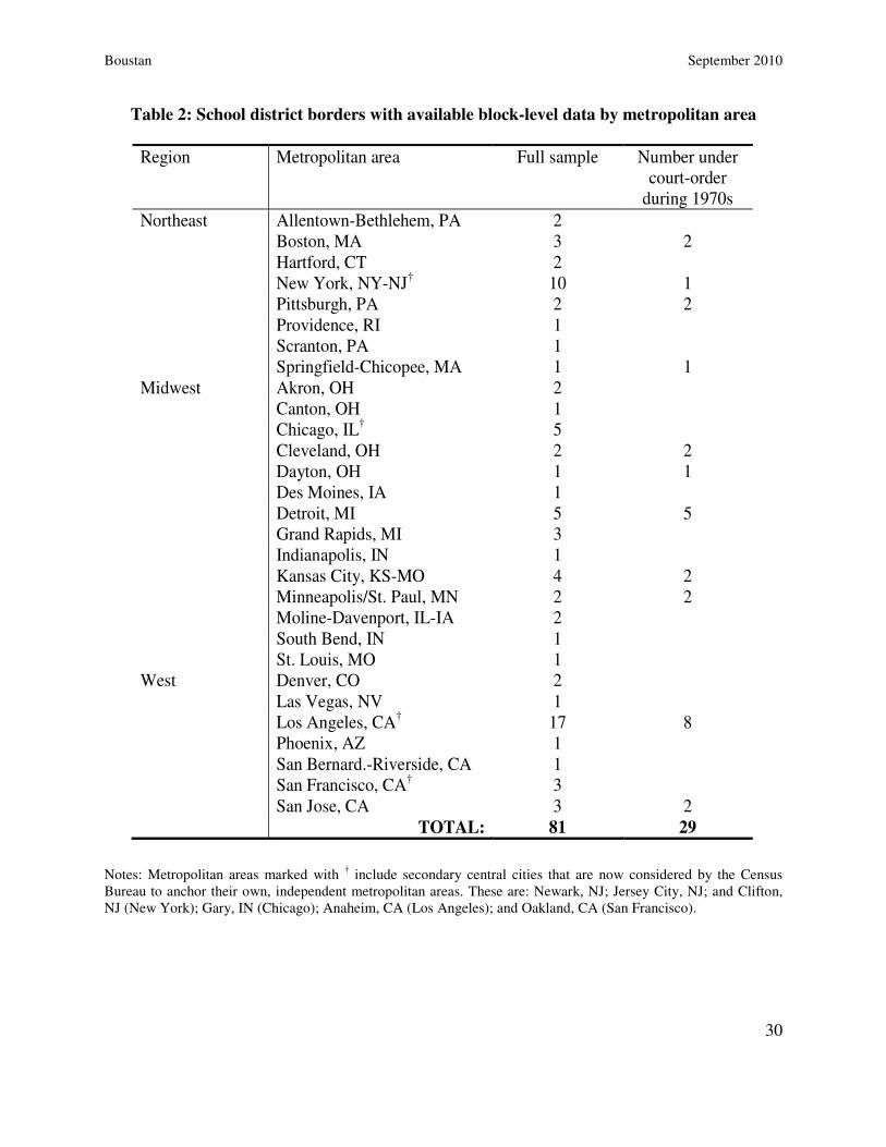
The dataset contains 81 city-suburban boundaries in 29 northern and western

metropolitan areas.9 Table 2 lists the metropolitan areas in the dataset and the number of borders

that each area contributes to the sample. The sample is evenly divided between the Northeast, the

Midwest and the West but slightly over-represents large, fragmented metropolitan areas with

populous suburbs. Los Angeles-Orange County, CA and New York City, NY-NJ, for example,

9 The number of district borders in the sample may seem small relative to the total number of such divisions in the typical urban area. The 15 metropolitan areas in the sample anchored by a large city (that is, one of the 50 largest cities in 1970) had an average of 10.5 borders, 6.7 of which had 10,000 or more residents and 4.9 of which were clear of any obvious obstruction. The average number of useable borders by metropolitan area in the sample is only 3.1 (median = 2.0) because the sample also includes areas anchored by smaller cities.


9

together contain a quarter of the non-southern metropolitan population in 1970 while accounting

for a third of the sample.10 I omit southern districts for three reasons. First, much of the school

desegregation activity in the South began in the 1960s, before the Census Bureau began sub-

dividing suburban areas into blocks. Second, many southern school districts cover an entire

county, incorporating both a central city and its suburban neighbors. Finally, the requirement to

desegregate was extended to many suburban school districts in the South.

The block-level dataset contains information on housing prices and rents and a small set

of housing quality measures from the Census of Housing. Due to confidentiality restrictions, the

mean housing value (rent) is only available for blocks containing at least five owner-occupied

(rental) units.11 Because desegregation may also affect the tenure decision, I also create a

measure of the average “user cost” of housing on the block. The user cost is calculated as a

weighted average of the annual rent paid by renters and the borrowing cost paid by homeowners

(= home value x interest rate).12

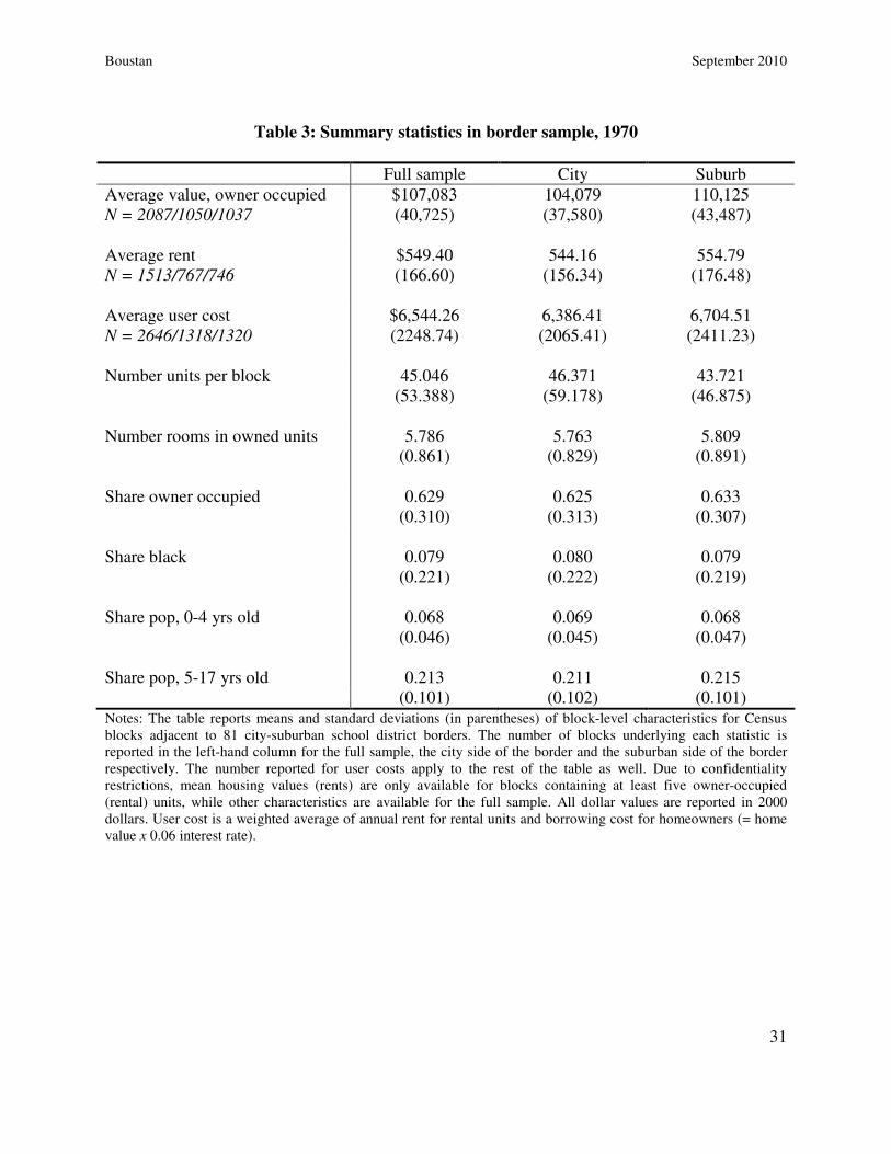
Table 3 presents summary statistics of these housing measures for the border sample.

Blocks on either side of the city-suburban border have typically “suburban” characteristics.

Nearly two-thirds of units were owner-occupied and residents on these blocks are

disproportionately white. Although eight percent of the residents on the average block were

black, over 80 percent of the blocks in the sample had no black residents at all. The racial

composition of sample blocks more closely resembles the average suburban district in the sample

(5.5 percent black) than the average city (14.5 percent black). The mean value of owner-

10 Many Ohio counties are unaccountably missing from the 1970 electronic block data. I limit coverage of Ohio to borders for which electronic data is available in 1970 and 1980. 11 Housing values are based on owner self-reports. Kain and Quigley (1972) argue that owner reports are reliable. However, self-reports may vary across district borders if some districts assess properties more regularly, thus providing owners with updated information. 12 I assume an interest rate of 6 percent, which is slightly lower than the average interest rate over the 1970s.


10

occupied units was slightly over $100,000 (in 2000 dollars) on both sides of the border and mean

monthly rents were around $550, figures that fall between the city and suburban means.

Although blocks on either side of the border are more similar to each other than they are to either

the typical city or suburban area, there are still discernable differences between them. In

particular, housing values were 5.7 percent higher on the suburban side of the border in 1970;

this difference is statistically significant.

B. School district variables

I collect data on the presence of desegregation court-orders by school district from the

State of Public School Integration website (Logan, 2004). The site contains the full text of

judicial decisions and enumerates each action that a district was required to take to counteract

desegregation. In the main specification, I measure the presence of a desegregation plan with a

dummy variable equal to one if the court required the district to engage in at least one remedial

step (PLAN). In alternative specifications, I also consider the number of remedial actions

required by the court-order or the years elapsed since the case was decided. Actions include steps

like redistricting school attendance areas, mandatory busing of students between schools, and the

creation of magnet schools. While the median court-order required that the school district engage

in two remedial steps, the number of steps ranges from one to ten.

The treatment group is made up of the 29 borders in the sample that divide an urban

district that faced a desegregation court-order in the 1970s from a suburban district that did not.

The other 52 borders constitute the control group. Of these, 40 borders did not receive a court-

order to desegregate on either side before 1980, 7 borders contain districts were both required to

desegregate over the 1970s, and 5 borders desegregated by early court-order in the 1960s.


11

Desegregation plans were intended to increase interracial contact in public schools. One

measure of the efficacy of these plans is the exposure index, which measures the share of the

student body at the average white student’s school that is black (or vice versa). The Office of

Civil Rights collected school-level enrollment data by race for all school districts in 1970 and a

sample of districts in 1980. The exposure index for district d is defined as:

Ed = (Σs=1…n [wsd · bsd/tsd]) / Wd (4)

where s indexes schools in the district. (bsd/tsd) measures the share of students at a given school

who are black or the number of black students divided by the total number of students enrolled at

that school. Ed calculates a weighted average of these black enrollment shares where the weights

are the number of white students at the school (wsd) and Wd indicates the number of white

students in the district as a whole.

The effect of desegregation on exposure to black peers may vary substantially across

households. Households living in school attendance areas whose local public school had a large

black enrollment share before desegregation may experience little increase in exposure to black

peers even with the implementation of a desegregation plan. In later specifications, I estimate

heterogeneous effects of desegregation plans on housing prices according to the black enrollment

share at the nearest high school in 1970. Without access to historical attendance area boundaries,

I assume that students would have been assigned to their nearest public school (as the crow

flies).13 I employ GIS software and school addresses from the 1970 Elementary and Secondary

General Information System (ELSEGIS) to match Census tracts to the nearest high school. The

mapping procedure is outlined in the Data Appendix.

13 The initial black enrollment share will be measured with error if school boards were able to successfully gerrymander school attendance areas before desegregation in order to prevent racially-mixed classrooms.


12

IV. Results

This section estimates the effect of court-ordered school desegregation on the demand for

urban residence by examining changes in the city-suburban housing price gap over the 1970s in

metropolitan areas with and without a court-ordered desegregation plan. White households may

have disliked school desegregation because of anxieties about mixed-race classrooms, concerns

about changes in peer quality, or objections to sending their children to non-neighborhood

schools. Because the block sample is disproportionately made up of white neighborhoods, the

estimates will recover the willingness to pay to avoid school desegregation for the marginal

white homeowner or renter.

A. Desegregation and exposure to cross-race peers

Desegregation court-orders were intended to increase racial balance across schools.

Reber (2005) demonstrates that the average desegregation plan successfully increased white

exposure to black peers and vice versa. I begin by replicating this finding in my sample to show

that the court-orders under study here were enforced (at least to some degree) and led to a

measurable change in school policy.

Table 4 compares changes in white exposure to black peers in urban districts that fell

under court-order during the 1970s with districts that avoided court supervision. At the beginning

of the decade, the black enrollment share at the average white student’s school was slightly lower

but not statistically different in districts that would fall under court-order (11.3 versus 12.6

percent), despite the fact that treated districts had a higher initial black population share. Over

the 1970s, average white exposure to black peers increased by 20 point in cities under court-

order but by only 5.5 points in cities that did not fall under court supervision. The difference-in-


13

differences estimator indicates that this 14.5 point difference in the change in exposure is

statistically significant and is robust to controlling for changes in total population and the black

population share over the 1970s.

B. Desegregation and housing values

Table 5 explores the effect of desegregation on the value of owner-occupied housing.

Column 1 begins by considering metropolitan areas whose central city received a court order to

desegregate during the 1970s. In 1970, the price for units on the city side of these borders was

already 4.7 percent lower than their suburban neighbors. This initial gap in housing prices could

reflect pre-existing disparities in school quality or in other municipal services, like police

protection. The presence of initial differences in housing prices underscores the importance of

being able to measure housing prices before and after the policy change.

From 1970 to 1980, after the imposition of court-ordered desegregation, the housing price

gap across these borders increased by 6.5 percentage points (equation 1). The declining relative

value of city housing likely reflects an aversion to school desegregation. This conclusion is

bolstered by the fact, illustrated in the second column, that the premium for suburban housing

remained steady, increasing by only 0.7 points at control borders over the 1970s (equation 2).

The difference-in-differences estimator indicates that the suburban price premium increased by

an additional 5.8 percentage points over the 1970s in metropolitan areas whose central city was

required to desegregate (equation 3).

The estimated decline in relative city housing prices may simply be a continuation of

trends from prior decades. The 1960s was a period of troubled race relations, prefaced by two

decades of black in-migration to central cities and resulting “white flight” (Collins and Margo,


14

2007; Boustan, 2010). The final row of Table 5 examines changes in the city-suburban housing

price gap across sample borders in the decade prior to the desegregation court-orders (1960 to

1970). I limit my attention to the 56 borders for which block-level data is available in 1960. Over

the 1960s, the city-suburban price gap expanded by 2 percentage points both in metropolitan

areas that fell under court-order in the 1970s and those that did not. The difference between these

two border types is negligible and not statistically significant. Therefore, it is unlikely that the

estimated change in housing prices is simply picking up long-run trends in urban demand.

For comparison, Table 6 estimates the effect of court-orders on the district-wide median

housing price for the 59 borders with available data in published Census volumes.14 The value of

owner-occupied housing in treated cities was already substantially lower than their suburban

counterparts in 1970 (18.5 percent). Over the decade, relative city prices declined by an

additional 10.5 percentage points in cities subject to court-ordered desegregation, compared to a

much smaller 1.7 percent in cities that were not. Altogether, relative housing prices fell by 12

percentage points more over the 1970s in cities that were subject to court-ordered desegregation.

The district-wide estimate of the willingness to pay to avoid school desegregation is

twice as large as the value obtained at the city-suburban border. The disparity in these estimates

may reflect differential trends in housing quality in the urban core relative to areas proximate to

the suburbs, which highlights the value of restricting the main analysis to blocks adjacent to the

district border. Alternatively, this gap could reflect different preferences between residents of

border areas and households in other parts of the metropolitan area. However, in this case, the

comparison between Tables 5 and 6 would imply that residents on the city side of border areas

14 The coefficient from the 1970 to 1980 difference-in-difference regression is qualitatively similar when I restrict the sample to either the 56 borders with available block data in 1960 or to the 59 borders with available district-level data.


15

were less averse to desegregation than was the typical city household; this pattern is unlikely to

hold given that households in border areas already selected to be close to the suburbs, perhaps to

avoid the heavily black neighborhoods in the urban core.

C. Desegregation and other housing and neighborhood outcomes

Table 7 examines the effect of desegregation on other neighborhood outcomes, including

rents, the user cost of housing, measures of housing quality and characteristics of local residents.

As before, I focus on the city-suburban gap in each outcome measured at the border. For brevity,

I do not present the level differences across borders in 1970 or 1980. Instead, the first column of

Table 7 reports the change in the city-suburban housing price gap over the 1970s in metropolitan

areas whose central city faced a desegregation court-order (equivalent to equation 1), the second

column presents this change for control areas (equation 2), and the third column compares the

two values (equation 3).

The monthly rent for rental units provides an additional measure of the market price of

housing. However, the effect of desegregation on owner-occupied and rental housing may differ

for two reasons. First, renters tend to be younger, less well-off, and less likely to have children,

all of which may lead them to have different preferences for local public goods. In addition,

housing prices incorporate expectations of future policy change between city and suburban

school districts, while rents capture a location’s value at a point in time. Given these factors, I

find that desegregation had a slightly smaller effect on rents, although, given the standard errors,

I cannot reject that the two estimates are the same. Over the 1970s, city rents fall by 6.6 percent

relative to their suburban neighbors across treated borders. The relative decline in city rents is


16

much more modest across control borders, resulting in a difference in differences estimate of a

4.0 percent decline in rents.

Due to data restrictions, only a subset of sample blocks have available data on average

rental rates (housing values). I calculate a measure of the user cost of housing for the full sample,

which is essentially a block-level weighted average of annual rents for rental units and annual

borrowing costs for owner-occupied units.15 Row 2 shows that the presence of a desegregation

plan is associated with a 7.1 percent reduction in the relative annual user costs of urban housing

in treated cities. Desegregation reduced both housing values and rents. Perhaps as a result, I find

little relationship between desegregation and owner-occupancy rates (row 3).

As prices fell, desegregation may have affected the financial return to home renovations

or maintenance. The only available measure of the quality of the housing stock is the number of

rooms in the typical unit. In areas under court-order to desegregate, the number of rooms in

suburban housing units increased by 0.12 of a room relative to the neighboring city (row 4). If all

home renovations consist of adding a single room, the difference-in-differences estimate

suggests that desegregation slowed the pace of renovation by 17 percent.

Beyond changes to the housing stock, desegregation may have induced a re-sorting of the

population at the local level, with households most opposed to the plan first to move out. White

households may have been more opposed to desegregation than black households because of

concerns about the effect of desegregation on peer quality. In addition, households with children

may have been particularly averse to living in a desegregated school district. As a result, districts

undergoing desegregation may have attracted more black residents and households without

children than neighboring blocks in the suburbs over the 1970s.

15 Note that the coefficient on user costs is not itself a weighted average of the housing price and rental estimates because many blocks have both owner-occupied and rental housing.


17

Despite the potential for re-sorting across borders, I find little relationship between

desegregation and either the racial composition or age distribution of the population in this

sample. The fifth row of Table 7 shows that the presence of a desegregation plan is associated

with a small and statistically insignificant increase in the probability of having a black neighbor.

The final row of Table 7 estimates the effect of desegregation on the share of residents made up

of school-aged children (5 to 17 years old). In both treatment and control areas, blocks on the

city side of the border experienced small relative declines in the presence of school-aged children

over the 1970s. Having a court-order did not lead to a differential decline in the size of the

school-aged population at city borders.16

V. Alternative specifications

Table 8 presents a series of robustness checks and alternative specifications for the

relationship between school desegregation and housing prices. The table’s first row reproduces

the baseline estimate, which finds that integration reduced housing prices by 5.8 percent. The

second row addresses the main threat to identification, namely other changes to central cities

over the 1970s that may have coincided with desegregation. Cities under court order were larger

and had a higher black population than cities that escaped court supervision (Table 1). A natural

candidate, then, for an omitted city-level variable is the incidence of race-related riot activity in

the 1960s and early 1970s. I use a city-level index of riot intensity proposed by Collins and

Margo (2007), which combines riot-related deaths, arrests, arsons and other forms of damage.

16 This pattern is consistent with Baum-Snow and Lutz’s (2008) finding that, outside the South, urban residents were more likely to respond to mandated school desegregation by shifting to private schooling rather than by leaving the central city. In this case, desegregation would not lead to out-migration from the city and resulting changes in household composition but would reduce the value of urban housing as the demand for the public schools bundled with city housing services falls.


18

For this application, I set the riot index equal to zero in all cities in 1970, despite the fact that

many riots occurred in the late 1960s, and assign the level of total riot activity over the period to

1980. Reassuringly, I find no effect of riot activity on housing prices from 1970 to 1980, either

because their consequences were already incorporated into housing prices by 1970, as Collins

and Margo’s results would suggest, or because the epicenter of the violence was far from the

suburban border. Most importantly for this context, adding a measure of riot activity has no

effect on magnitude or precision of desegregation estimate.

The third row of Table 8 augments the price regression with a control for the average

number of rooms on the block. In this case, desegregation court-orders reduce housing prices by

4.0 percent, implying that around 30 percent of the total relationship between desegregation and

housing prices can be explained by changes in the underlying housing stock. Readers may prefer

this value as the best hedonic estimate of the willingness to pay to avoid school integration given

that it controls for other observed differences in housing quality. In the fourth row of Table 8, I

drop the five borders that faced early desegregation plans from the control group. Doing so

reduces the coefficient of interest to 4.9 percent, which remains significant at the 10 percent

level. The results are qualitatively unchanged in regressions that weight each block or each

border equally (rows 5 and 6), rather than weighting by the number of owner-occupied units on

the block.

In the main specification, I group all desegregation court-orders into a single category

and compare cities that faced a court-order in the 1970s to those that did not. In the seventh row,

I instead count the number of required remedies contained in the court-order. Remedies include

actions like rezoning school attendance areas, transferring students between schools, busing

students between schools or creating a magnet school. The coefficient implies that each required


19

step reduced housing values by 1.9 percent. According to this estimate, a desegregation plan with

the median number of steps (two) would lead to a 3.8 percent reduction in housing values, which

is lower than the baseline estimate. This comparison suggests that the first step in a new plan had

a larger effect on housing values than did incremental steps added to an existing plan.

School districts may have phased in the reforms required by a court-order over a number

of years. In this case, we may expect the effect of a desegregation plan on housing values to

accumulate over time. On the other hand, as soon as a court-order is handed down, the intended

policy changes can be anticipated by the public and, therefore, any effect on the demand for

residence in the school district may occur immediately. The eighth row of Table 8 replaces the

dummy variable for the presence of a desegregation plan with a continuous variable indicating

the years since the court-order was handed down. Housing values decline by 1.3 percent for

every year since the court order was issued. This coefficient implies that the 5.9 percent decline

in housing values estimated is reached around five years after the plan is first announced.

In the ninth row, I restrict my attention to blocks whose residents are at least 98 percent

white. School desegregation has a larger negative effect on housing prices in this sub-sample (8.4

percent). The final rows of Table 8 allow for a heterogeneous response to desegregation on the

basis of the initial black enrollment share at the nearest high school. A district-wide

desegregation plan would have little effect on blocks that were already assigned to a racially

integrated school. The ninth row interacts the indicator for the presence of a desegregation plan

with the black enrollment share in the nearest high school in 1970. Desegregation reduces

housing values by 13.2 percent in areas of the city that otherwise would have attended an all-

white high school (that is, the blocks for which the local high school had a black enrollment

share of zero in 1970). As the initial black enrollment share of the local high school increases,


20

the estimated effect of desegregation on housing values declines. The coefficients suggest that

desegregation would have had no effect on housing values in areas that were assigned to a high

school with a 40 percent black enrollment share in 1970 (= -0.132 + [0.336 · 0.4]).17

VI. Interpretation

This section highlights three implications of the relationship between school

desegregation and urban housing prices. First, I argue that court-ordered desegregation reduced

the tax base of central cities, imposing a fiscal externality on city residents. Second, by

comparing my estimate with others from the literature, I show that the willingness to pay to

avoid school desegregation can be attributed both to concerns about cross-race peers and to

preferences for neighborhood schools. Finally, I argue that the housing price estimate suggests

that the marginal northern homeowner was substantially less resistant to desegregation than was

the median southern voter, in the sense that she would have needed less monetary compensation

in order to accept racial desegregation in local schools.

A. Tax revenue and fiscal externalities

The typical desegregation plan reduced housing values and rents in an urban school

district. As a result, desegregation reduced the residential tax base in urban school districts

relative to their neighboring suburbs. The average school district in the sample allocated $4,000

per pupil in educational expenditures (in 2000 dollars) and relied on residential property taxes for

17 There is substantial variation in the black enrollment share at the nearest high school across borders (mean gap = 15 pp; standard deviation = 23 pp). I find a similar effect on housing prices when I interact the presence of a desegregation order with the difference between the district-wide black enrollment share and enrollment at the local high school, a measure that provides a sense of how much the local school would have had to change in order to be in compliance with the court order.


21

75 percent of total revenue. Under various assumptions about the effect of desegregation on

housing values in black neighborhoods, my estimates suggest that desegregation would have

reduced the residential tax base by 4.9 to 6.0 percent.18 A decline of this magnitude would

translate into a $147 to $180 reduction in revenue per pupil assuming a constant property tax

rate.19

The full effect of desegregation on available resources per pupil depends on the

relationship between desegregation and both tax revenues and schooling costs. If desegregation

required new expenditures, such as additional buses or higher teacher salaries, the estimated

decline in available resources per pupil would understate the true decline. In contrast, if the

policy change resulted in a net loss of student enrollments in urban schools, this value would be

an overestimate. Furthermore, the research design in this paper can only identify changes in

urban housing prices relative to neighboring suburbs. Therefore, while it is clear that school

integration exacerbated inequities in school resources between cities and suburbs, we cannot

conclude definitively that the urban tax base experienced an absolute decline.

B. Cross-race peers and neighborhood schools

The typical desegregation plan altered the mechanism by which students were assigned to

schools. In order to comply with desegregation orders, school districts could no longer place all

18 The average decline in the residential tax base is a weighted average of changes in user costs in white and black neighborhoods. Given that residents on sample blocks are predominately white, I assume that my estimate indicates the change in housing prices in white neighborhoods. 84 percent of Census tracts in the median sample city were predominately white (defined as less than two percent black). If housing values were unchanged in black neighborhoods following desegregation, the residential tax base would have declined by 6.0 percent (= 0.16 · 0.000 + 0.84 · -0.071). If, instead, housing values increased in black neighborhoods by as much as they declined in white neighborhoods, the residential tax base would have declined by 4.9 percent (= 0.16 · 0.071 + 0.84 · -0.071). This calculation uses the user cost of housing estimates from Table 8, row 2. 19 Of course, cities were free to respond to this decline in the tax base by increasing the property tax rate, thereby holding constant the revenue collected per pupil. In that case, the cost of the unfunded mandate would have been borne broadly by property owners and renters, rather than only by households with school-aged children.


22

students in the nearest school. Rather, many white students were reassigned to schools in

predominately black neighborhoods and vice versa. Comparing my results with estimates from

the literature, I infer that objections to school desegregation were driven by more than just fears

about cross-race classrooms or concerns about peer quality but also reflect an aversion to the

assignment mechanism by which desegregation was achieved.

Kane, Riegg and Staiger (2006) compare housing prices on either side of elementary

school attendance area boundaries in Charlotte-Mecklenberg, NC, while controlling for distance

to school. According to their estimate, the increase in black enrollment associated with the

typical desegregation plan would cause housing prices to decline by 3.8 percent.20 By this

measure, two-thirds of the estimated housing price response to school desegregation can be

attributed to concern about mixed-race classrooms and associated changes in peer quality (=

3.8/5.9). The remainder of the estimated price response is likely due to concerns about school re-

assignment. Bogart and Cromwell find that assignment to a non-neighborhood school reduces

housing prices by 7.5 percent. The residual change in housing prices would therefore imply that

around 30 percent of sample households faced school re-assignment (= [5.9-3.8]/7.5), a value

consistent with qualitative accounts of how desegregation was implemented.

C. A revealed preference approach to the history of Civil Rights

Existing histories of the Civil Rights era generalize about the popular response to school

desegregation on the basis of the writings and actions of the most outspoken members of

20 Kane and co-authors estimate that a 10 percentage point increase in black enrollment share leads to a 2.6 percent decline in housing prices, suggesting that the 14.5 percentage point increase in black enrollment associated with the typical plan in my sample (Table 4, row 2) would lead to a 3.8 percent decline in housing prices. A related study is Clotfelter (1975), who compares housing prices across high school attendance areas following the desegregation of Atlanta schools.


23

society.21 These views – whether of angry segregationists who gathered to block the

desegregation of Central High in Little Rock, AR or of crusading integrationists who marched in

Selma, AL – may not be representative of the average resident. In contrast, this paper seeks to

elicit typical attitudes toward school desegregation by studying the behavior of the marginal

homeowner or renter.

In a related approach, Cascio, et al. (2010) study a large sample of southern school

districts. Title I of the 1965 Elementary and Secondary Education Act provided federal funding

for K-12 education nationwide. In order to be eligible for funding, school districts could not

maintain segregated schools. The authors reason that, by accepting the offer of federal funding,

school districts reveal the price at which their median voter was willing to forgo segregated

schools. To be in compliance, districts needed to increase the black enrollment share at the

average white student’s school by around four percentage points. Cascio, et al. estimate that the

typical southern district was willing to engage in this amount of desegregation for $1000 per

pupil per year of federal funding (in 2000 dollars).

To compare my results with Cascio, et al., I convert housing prices into dollars per pupil.

By my estimate, a four percentage point increase in black enrollment share is associated with a

2.0 percent decline in the user cost of housing, or a $130 reduction in annual user costs for the

average housing unit (=$6,508 · 0.020).22 Converting this value into dollars per child yields an

21 A non-exhaustive list of the vast historical literature on responses to desegregation includes Carter, 1995; Gaston, 1998; Webb, 2005; Sokol, 2006 and Crespino, 2009. 22 The typical plan in my sample increased black enrollment share by 14.5 percent (Table 4) and reduced user costs by 7.1 percent (Table 8). By this estimate, the 4 percentage point increase in black enrollment share associated with Title I funding would lead user costs to fall by 2.0 percent. User costs is the most relevant metric for this calculation because it combines the preferences of home-owners and renters.


24

annual payment of $234 per child, around one-fourth of the federal payments required to induce

the typical southern school district to begin the desegregation process.23

By this metric, the median southern voter appears to have been four times as resistant to

school desegregation as the marginal resident in the North.24 Despite potential differences

between the median voter and the marginal resident as bellwethers of “average” tastes, it appears

that the typical southerner was substantially more opposed to desegregation than was the typical

northerner. However, this gap is not as large as we might expect based on the case study

evidence alone.

VII. Conclusion

The integration of public schools by race was one of the most important changes to the

American educational system in the twentieth century. The Supreme Court first required school

districts to address the de facto school segregation associated with historical patterns of

residential location by race in the mid-1970s. The Court considered extending this obligation to

predominately white suburban areas, but ultimately rejected this possibility in the 1974 Miliken

v. Bradley decision. Therefore, outside of the South, court-ordered desegregation was applied

only to central cities.

As a result, the integration of public schools changed the value of urban residence in the

North and West. Urban schools became more racially diverse and students were often reassigned

23 The average block had 45 housing units and 25 school-aged children (5-17 years old). 24 This comparison could understate regional differences because northern desegregation plans often required school reassignment while southern plans did not. However, the comparison could also overstate the typical southerner’s distaste for integration for two reasons. First, residents most concerned about integration may have been most likely to vote in school board elections. Second, the Cascio, et al. paper generates variation in the size of federal grants by comparing rich and poor districts in states with greater and less school spending. Therefore, the marginal district that is indifferent about accepting the federal funding or not will be a rich district in an ungenerous state whose residents may have been more opposed to integration than the southern average.


25

to non-neighborhood schools in order to achieve the necessary racial mix. I show in this paper

that this process of school desegregation resulted in a decline in the demand for urban residence.

Housing prices and rents in cities under court-order fell by six percent relative to their

neighboring suburbs. The associated reduction in the urban tax base created a fiscal externality

for remaining residents of central cities.

Changes in housing prices reveal the marginal home owner’s willingness to pay to avoid

school desegregation. This value converts the average disapproval of school desegregation into a

dollar value that can then be compared to other programs, time periods, or regions. Cascio, et al.,

for instance, estimate that the typical southern district would have engaged in a token amount of

desegregation for a payment of $1,200 per pupil. By this measure, northern residents appear to

be four times less averse to desegregation than the median southern voter. Such a revealed

preference-based measure contributes to our understanding of the history of school desegregation

and of the Civil Rights era more broadly.


26

Data Appendix

Pairing each Census block with the nearest high school proceeds in three steps: 1. 1970 street addresses for schools in sample districts are obtained from the Elementary and Secondary General Information System (ELSEGIS). I identify academic high schools as those that contain grades 9-12 or 10-12 and do not include the words “manual,” “technical” or “vocational” in their name. Using GIS software, I locate these schools using the 2000 Census electronic road maps (http://www.esri.com/data/download/census2000_tigerline/). This process accurately geocoded over 90 percent of the schools in the sample. I checked the names and addresses of all unmatched schools using on-line resources. In some cases, road names had changed from 1970 to 2000 and could be edited by hand; in others, schools appears to have closed in the intervening three decades. 2. In a separate GIS layer, I map the centroid of Census tracts that contribute blocks to the sample. I then calculate the distance between Census tracts and high schools within the same district and select the high school with the minimum distance to be the assigned school for that area. 3. The Office of Civil Rights collected data on the racial composition of enrolled students by school. I match the OCR data with the ELSEGIS addresses using a cross-walk between the school identifiers. Districts with multiple tracts along one border area can match to more than one high school. In this cases, I assign the average racial composition of the two closest high schools to that area.


27

Bibliography

Angrist, Joshua D. and Kevin Lang. 2004. “Does School Integration Generate Peer Effects? Evidence from Boston’s Metco Program.” American Economic Review 94(5): 1613-1634.

Ashenfelter, Orley, William Collins, and Albert Yoon. 2006. “Evaluating the Role of Brown v.

Board of Education in School Equalization, Desegregation, and the Income of African Americans.” American Law and Economics Review 8(2): 213-248.

Baum-Snow, Nathaniel. 2007. “Did Highways Cause Suburbanization?” Quarterly Journal of Economics 122: 775-805. Baum-Snow, Nathaniel and Byron Lutz. 2008. “School Desegregation, School Choice and

Changes in Residential Location Patterns by Race.” Manuscript. Black, Sandra. 1999. “Do Better Schools Matter? Parental Valuation of Elementary Education.”

Quarterly Journal of Economics. 114(2): 577-599.

Bogart, William T. and Brian A. Cromwell. 2000. “How Much is a Neighborhood School Worth?” Journal of Urban Economics, 47: 280-305.

Boustan, Leah Platt. 2007. “Escape from the City? The Role of Race, Income, and Local Public

Goods in Post-War Suburbanization.” NBER Working Paper No. 13311. -----------------------. 2010. “Was Postwar Suburbanization ‘White Flight’? Evidence from the

Black Migration,” Quarterly Journal of Economics, 417-43. Carter, Dan. 1995. The Politics of Rage: George Wallace, the Origins of the New Conservatism,

and the Transformation of American Politics. Baton Rouge: LSU Press. Cascio, Elizabeth, Nora Gordon, Ethan Lewis and Sarah Reber. 2010. “Paying for

Progress: Conditional Grants and the Desegregation of the South.” Quarterly Journal of

Economics 125(1): 445-82. Clotfelter, Charles T. 1975. “The Effect of School Desegregation on Housing Prices.” Review of

Economics and Statistics 57: 395-404. Coleman, James S. 1975. “Trends in Social Segregation: 1968-73.” Urban Institute Paper No.

722-03-01. Collins, William J. and Robert A. Margo. 2007. “The Economic Aftermath of the 1960s Riots:

Evidence from Property Values.” Journal of Economic History. Crespino, Joseph. 2009. In Search of Another Country: Mississippi and the Conservative

Counterrevolution. Princeton: Princeton University Press.


28

Figlio, David and Maurice Lucas. 2004. “What’s in a Grade? School Report Cards and the Housing Market.” American Economic Review, 94(3), p. 591-604.

Gaston, Paul M. 1998. The Moderates’ Dilemma: Massive Resistance to School Desegregation

in Virginia. Charlottesville: University Press of Virginia. Guryan, Jonathan. 2004. “Desegregation and Black Dropout Rates,” American Economic

Review, 94(4): 919-943. Hoxby, Caroline and Gretchen Weingarth. 2005. “Taking Race Out of the Equation: School

Reassignment and the Structure of Peer Effects,” Manuscript. Kain, John F. and John M. Quigley. 1972. “Housing Market Discrimination, Home Ownership,

and Savings Behavior.” American Economic Review, 62: 263-277.

Kane, Thomas J. Douglas O. Staiger and Gavin Samms. 2003. “School Accountability Ratings and Housing Values.” In William Gale and Janet Rothenberg Pack (eds.) Brookings-

Wharton Papers on Urban Affairs, pp. 83-138. Kane, Thomas, Stephanie Riegg, and Douglas Staiger. 2006. “School Quality, Neighborhoods

and Housing Prices.” American Law and Economics Review 9(2): 183-212. Logan, John. 2004. “Desegregation Court Cases.” The State of Public School Integration. Brown

University. <http://www.s4.brown.edu/schoolsegregation/desegregationdata.htm.> Lutz, Byron. 2005. “Post Brown v. the Board of Education: The Effects of the End of Court-

Ordered Desegregation.” Finances and Economics Discussion Series, Federal Reserve Board, 2005-64.

Reber, Sarah J. 2005. “Court-Ordered Desegregation: Successes and Failures in Integration Since

Brown.” Journal of Human Resources, 40(3): 559-590. ----------------. Forthcoming. “School Desegregation and Educational Attainment for Blacks.”

Journal of Human Resources. Sokol, Jason. 2006. There Goes My Everything: White Southerners in the Age of Civil Rights.

New York: Knopf. Webb, Clive, ed. 2005. Massive Resistance: Southern Opposition to the Second Reconstruction.

Oxford: Oxford University Press. Welch, Finis and Audrey Light. 1987. New Evidence on School Desegregation. Washington,

DC: U.S. Commission on Civil Rights.


29

Table 1: Initial characteristics of urban school districts, 1970

Under order during 1970s

No order during 1970s

Difference

ln (population) 13.172 12.071 1.100 (1.307) (0.922) (0.334) Share black 0.189 0.130 0.059 (0.127) (0.136) (0.043) ln(median income) 10.718 10.716 0.002 (0.139) (0.132) (0.043) Share poverty 0.093 0.085 0.009 (0.027) (0.035) (0.010) Share college degree 0.122 0.104 0.017 (0.093) (0.056) (0.022) Notes: The regressions compare the 13 cities that received a desegregation court-order during the 1970s to the 36 cities that did not. Characteristics are measured in 1970.


30

Table 2: School district borders with available block-level data by metropolitan area

Notes: Metropolitan areas marked with † include secondary central cities that are now considered by the Census Bureau to anchor their own, independent metropolitan areas. These are: Newark, NJ; Jersey City, NJ; and Clifton, NJ (New York); Gary, IN (Chicago); Anaheim, CA (Los Angeles); and Oakland, CA (San Francisco).

Region Metropolitan area Full sample Number under court-order

during 1970s

Northeast Allentown-Bethlehem, PA 2 Boston, MA 3 2 Hartford, CT 2 New York, NY-NJ† 10 1 Pittsburgh, PA 2 2 Providence, RI 1 Scranton, PA 1 Springfield-Chicopee, MA 1 1 Midwest Akron, OH 2 Canton, OH 1 Chicago, IL† 5 Cleveland, OH 2 2 Dayton, OH 1 1 Des Moines, IA 1 Detroit, MI 5 5 Grand Rapids, MI 3 Indianapolis, IN 1 Kansas City, KS-MO 4 2 Minneapolis/St. Paul, MN 2 2 Moline-Davenport, IL-IA 2 South Bend, IN 1 St. Louis, MO 1 West Denver, CO 2 Las Vegas, NV 1 Los Angeles, CA† 17 8 Phoenix, AZ 1 San Bernard.-Riverside, CA 1 San Francisco, CA† 3 San Jose, CA 3 2 TOTAL: 81 29


31

Table 3: Summary statistics in border sample, 1970

Full sample City Suburb Average value, owner occupied $107,083 104,079 110,125 N = 2087/1050/1037 (40,725) (37,580) (43,487) Average rent $549.40 544.16 554.79 N = 1513/767/746 (166.60) (156.34) (176.48) Average user cost $6,544.26 6,386.41 6,704.51 N = 2646/1318/1320 (2248.74) (2065.41) (2411.23) Number units per block 45.046 46.371 43.721 (53.388) (59.178) (46.875) Number rooms in owned units 5.786 5.763 5.809 (0.861) (0.829) (0.891) Share owner occupied 0.629 0.625 0.633 (0.310) (0.313) (0.307) Share black 0.079 0.080 0.079 (0.221) (0.222) (0.219) Share pop, 0-4 yrs old 0.068 0.069 0.068 (0.046) (0.045) (0.047) Share pop, 5-17 yrs old 0.213 0.211 0.215 (0.101) (0.102) (0.101) Notes: The table reports means and standard deviations (in parentheses) of block-level characteristics for Census blocks adjacent to 81 city-suburban school district borders. The number of blocks underlying each statistic is reported in the left-hand column for the full sample, the city side of the border and the suburban side of the border respectively. The number reported for user costs apply to the rest of the table as well. Due to confidentiality restrictions, mean housing values (rents) are only available for blocks containing at least five owner-occupied (rental) units, while other characteristics are available for the full sample. All dollar values are reported in 2000 dollars. User cost is a weighted average of annual rent for rental units and borrowing cost for homeowners (= home value x 0.06 interest rate).


32

Table 4: School desegregation and white exposure to black peers

Dependent variable = White exposure to black peers

Mean/standard deviation Under court-order

during 1970s Not under court order

during 1970s Difference

1970 0.113 0.126 -0.012 (0.067) (0.114) (0.034) 1980 0.313 0.181 0.132 (0.206) (0.119) (0.053) ∆ 1970-1980 0.145 (0.063) ∆ 1970-80 with controls 0.135 (0.039) Notes: The sample includes city districts for which there is school-level data on racial composition in 1970 and 1980. The regressions compare the 13 cities that received a desegregation court-order during the 1970s to the 24 cities with available data that did not. The difference-in-differences specification in the fourth row controls for the black population share and logarithm of total population in the district.


33

Table 5: School desegregation and relative city housing prices at the district border,

1960-80

Dependent variable = ln(housing value)

Under court-order during 1970s

Not under order during 1970s

Difference

1970 -0.047 -0.026 -0.021 (0.014) (0.015) (0.020) 1980 -0.097 -0.023 -0.073 (0.028) (0.022) (0.035) ∆ 1970-1980 -0.065 -0.007 -0.058 (0.024) (0.015) (0.028) Pre-trend: ∆ 1960-1970 -0.023 -0.022 -0.001 (0.013) (0.017) (0.022) Notes: Standard errors are reported in parentheses and clustered by school district. In rows 1 and 2, cells contain coefficients from regressions of block-level housing values on an indicator variable for being in the central city in a given decade (1970 or 1980). Row 3 reports coefficients for regressions of changes in housing prices from 1970 to 1980 on the interaction between being in the central city and in the 1980 Census year (equations 1-3 in the text). Row 4 conducts the same regression for the previous decade (1960 to 1970). Note that the coefficients in row 3 are not equivalent to the difference between the coefficients in rows 1 and 2 because the regressions underlying row 3 also include side of border fixed effects. All regressions are weighted by the number of owner-occupied units on the block. For rows 1 to 3, the sample includes Census blocks adjacent to 81 city-suburban school district borders in 1970 and 1980. Data on housing values are only available for blocks containing at least five owner-occupied units. Regressions in row 3 contain 4386 observations, 2087 blocks from 1970 and 2299 blocks from 1980. Row 4 contains Census blocks adjacent to the 56 city-suburban borders with block-level data in 1960 (2495 observations, 1010 blocks from 1960 and 1485 blocks from 1970).


34

Table 6: School desegregation and relative city housing prices for the district as a whole

Dependent variable = ln(median housing value)

Under court-order during 1970s

Not under order during 1970s

Difference

1970 -0.185 -0.073 -0.112 (0.052) (0.036) (0.063) 1980 -0.290 -0.090 -0.200 (0.072) (0.050) (0.086) ∆ 1970-1980 -0.142 -0.022 -0.120 (0.044) (0.020) (0.040) Notes: Standard errors are reported in parentheses. See the notes to Table 5 for details on the specification. The sample consists of school districts along the 59 borders for which housing price data is available in published Census volumes in 1970 and 1980.


35

Table 7: The effect of desegregation on other housing and neighborhood outcomes

Court-order in 1970s ∆ 1970-80

No order in 1970s ∆ 1970-80

Difference Order vs. no order

ln(rent) -0.066 -0.027 -0.040 (0.024) (0.021) (0.030) ln(user cost) -0.102 -0.030 -0.071 (0.025) (0.021) (0.031) Share owner occupied -0.014 0.002 -0.017 (0.021) (0.009) (0.023) Number of rooms -0.115 0.050 -0.166 (0.076) (0.056) (0.094) Share black 0.020 0.003 0.017 (0.019) (0.010) (0.021) Share 5-17 years old -0.008 -0.008 0.000 (0.011) (0.004) (0.012) Notes: Standard errors are reported in parentheses and clustered by school district. The sample includes Census blocks adjacent to 81 city-suburban school district borders in 1970 and 1980. See notes to Table 5 for further details on the sample and regression specification.


36

Table 8: Alternate specifications: Desegregation and housing values

Dependent variable = ln(housing value)

Coefficient (1) Baseline effect -0.058 (0.028) (2) Control for riot activity in city -0.060 (0.028) (3) Control for number of rooms on block -0.040 (0.026) (4) Drop borders with early plans (in 1960s) -0.049 (0.028) (5) Weight each block equally -0.058 (0.027) (6) Weight each border equally -0.059 (0.029) (7) RHS = Number of steps in court-order -0.019 (0.003) (8) RHS = Number of years since order passed -0.013 (0.004) (9) Limit to blocks less than 2% black -0.084 (0.027) (10) Interaction with local high school Court-order during 1970s -0.132 (0.025) Order during 1970s x Black enroll share, 1970 0.336 (0.127) Notes: Standard errors are reported in parentheses and clustered by school district. The sample includes Census blocks adjacent to 81 city-suburban school district borders in 1970 and 1980. See notes to Table 5 for further details on the sample and regression specification. The Data Appendix explains how Census blocks were paired with their nearest high school in 1970. School-level racial composition data is from the Office of Civil Rights.

Documents

School Desegregation and Urban Change: Evidence … Joshua Angrist, Nathaniel Baum-Snow, Sandra Black, ... of Kansas and the KALER group at UCLA. The views expressed herein are those