DI

SC

US

SI

ON

P

AP

ER

S

ER

IE

S

Forschungsinstitut zur Zukunft der ArbeitInstitute for the Study of Labor

School Access, Resources, and Learning Outcomes:Evidence from a Non-formal School Programin Bangladesh

IZA DP No. 5659

April 2011

Hai-Anh DangLeopold SarrNiaz Asadullah

School Access, Resources, and Learning Outcomes: Evidence from a Non-formal

School Program in Bangladesh

Hai-Anh Dang World Bank

Leopold Sarr

World Bank

Niaz Asadullah University of Reading

and IZA

Discussion Paper No. 5659 April 2011

IZA

P.O. Box 7240 53072 Bonn

Germany

Phone: +49-228-3894-0 Fax: +49-228-3894-180

E-mail: iza@iza.org

Any opinions expressed here are those of the author(s) and not those of IZA. Research published in this series may include views on policy, but the institute itself takes no institutional policy positions. The Institute for the Study of Labor (IZA) in Bonn is a local and virtual international research center and a place of communication between science, politics and business. IZA is an independent nonprofit organization supported by Deutsche Post Foundation. The center is associated with the University of Bonn and offers a stimulating research environment through its international network, workshops and conferences, data service, project support, research visits and doctoral program. IZA engages in (i) original and internationally competitive research in all fields of labor economics, (ii) development of policy concepts, and (iii) dissemination of research results and concepts to the interested public. IZA Discussion Papers often represent preliminary work and are circulated to encourage discussion. Citation of such a paper should account for its provisional character. A revised version may be available directly from the author.

IZA Discussion Paper No. 5659 April 2011

ABSTRACT

School Access, Resources, and Learning Outcomes: Evidence from a Non-formal School Program in Bangladesh*

This study reports evidence from an unusual policy intervention – The Reaching Out of School Children (ROSC) project – in Bangladesh where school grants and education allowances are offered to attract hard-to-reach children to schools comprised of a single teacher and a classroom. The operating unit cost of these schools is a fraction of that of formal primary schools. We use panel data to investigate whether ROSC schools are effective in raising enrolment and learning outcomes. Our findings suggest that there is a modest impact on school participation: ROSC schools increase enrolment probability between 9 and 18% for children in the two age cohorts 6-8 and 6-10. They perform as well as non-ROSC schools in terms of raising test scores, and even have positive impacts on academically stronger students. There is also strong evidence of positive externalities on non-ROSC schools in program areas. These results point to the effectiveness of a new model of non-formal primary schools that can be replicated in similar settings. JEL Classification: I21, O10 Keywords: non-formal school, impact evaluation, multiple treatments, learning outcomes Corresponding author: Hai-Anh Dang South Asia Human Development Sector World Bank 1818 H Street NW, MC3-311 Washington, DC 20433 USA E-mail: hdang@worldbank.org

* We thank Amit Dar, Celine Ferre, Deon Filmer, Dilip Parajuli, Christel Vermeersch, Liang Choon Wang, and participants at a seminar at the World Bank for comments on previous versions of this paper. The findings and interpretations in this paper do not necessarily reflect the views of the World Bank or its Executive Directors.

1

I. Introduction

Despite their seemingly indispensable roles in promoting student educational

outcomes, there have been mixed results on the impacts of school supply and resources on

access and learning outcomes (Hanushek, 2006). Findings from recent rigorous impact

evaluation studies suggest that this is particularly the case for developing countries. On

one hand, providing educational inputs such as textbooks (Glewwe, Kremer and Moulin,

2009), flip charts (Glewwe et al., 2004), and reduced teacher-pupil ratios (Duflo, Dupas,

and Kremer, 2010) were generally found to have either no or very limited impacts on

student test scores. On the other hand, other inputs such as remedial education programs

(Banerjee et al., 2007), extra after-school classes (Banerjee et al., 2010), free school

uniform (Evans, Kremer, and Ngatia, 2008), and reduced student fees and scholarship

(Kremer, Miguel, and Thorton, 2009) were found to increase student reading skills and

test scores and/ or decrease drop-out rates. Even the building of new schools does not

always lead to large gains in school enrolment rates (Filmer, 2007). It appears that no

consensus has been reached on the best school (policy) interventions to expand

educational opportunities in developing countries.1

Even in the case such a consensus exists, providing more inputs into the existing

systems may not bring the best outcomes. Institutional issues with educational systems in

developing countries such as corruption, lack of transparency, and inefficient use of

resources may severely impair the effectiveness of increased school resources (Glewwe

and Kremer, 2006). In response to these problems, an alternative schooling model has

1 There is conflicting evidence as well about other school supply interventions such as teacher performance pay, which is found to have positive impacts on test scores in India (Muralidharan and Sundararaman, 2009) but no or limited impacts in Kenya (Glewwe, Ilias, and Kremer, 2010). See also Glewwe and Kremer (2006) and Kremer and Holla (2009) for more general review of the literature on the impacts of school inputs, and Dang and Rogers (2008) for a review on the impacts of extra tutoring classes.

2

been introduced: the non-formal schooling system. Starting in the late 1970s with the

Escuela Nueva (New School) program in rural Colombia (Psacharopolous, Rojas, and

Velez, 1993; McEwan, 1998), the non-formal schooling movement is gaining more

popularity and has spread to many developing countries including the BRAC (Bangladesh

Rural Advancement Committee) primary school program in Bangladesh in the mid-1980s

(Chabbot, 2006), the Community School program in Egypt in the early 1990s (Farrell,

2004), and the School for Life program in Ghana in the late 1990s (Hartwell, 2006).

In spite of their different names, these programs appear to share at least three common

characteristics: they are usually operated by non-state providers (in particular, NGOs)

with strong community participation, they have low operational costs, and they cater to

vulnerable and hard-to-reach students who were excluded for various reasons from the

formal education system.2 It is notable that these programs are currently spreading to

urban areas, post-primary schooling levels, and formal public schools as well. The

Reaching Out-Of-School Children (ROSC) program we evaluate in this paper is a

particular example where, inspired by the ‘success’ of the BRAC model,3 the Government

of Bangladesh brought this model into the formal schooling system and expanded it on a

large scale. Since 2005, ROSC has provided more than 15,000 schools (learning centers)

serving over 500,000 educationally disadvantaged children in the poorest 60 Upazilas

2 See Farrell and Hartwell (2008) and Ahmed (2008) for two recent (and qualitative) reviews of non-formal school programs. 3 A BRAC school is a school consisting of one teacher and one classroom that caters to out-of-school (and usually marginalized) children which is operated by the NGO BRAC. Although BRAC schools and government public schools teach the same the same competency-based curriculum, Chabbott (2006) points out three key operational differences between these schools: i) student intake occurs every four years at the former but annually at the latter, ii) the average class size is 25 to 33 students at the former, but around twice higher at 61 students at the latter, and iii) while the former averages 4,091 contact hours per primary cycle, the corresponding figure at the latter is lower at 4,046. At the same time, BRAC schools have higher attendance rates (96 percent) and completion rates (94 percent) than government public schools (61 and 67 percent respectively), and BRAC students have higher test scores across several different subjects including life skills, reading, writing, and numeracy. Chabbott also estimates the cost per BRAC school completer is $84, around one third that of $246 for government public school.

3

(sub-districts) in Bangladesh. The program is currently being expanded to include 30

additional Upazilas.

While these non-formal education programs have reached tens of thousands of schools

and millions of students all over the world, there are very few studies that rigorously

evaluate their impacts on enrolment and learning outcomes. Furthermore, the existing few

studies provide mixed results. The most comprehensive assessment of the relative

performance of BRAC schools in Bangladesh finds that non-formal schools in Bangladesh

are effective in raising female enrolment and test scores in rural areas (Sukontamarn,

2006). In the absence of panel data, Sukontamarn relies on cross-sectional data and

combines information on child year of birth and year of BRAC school establishment in

the village to compare the impacts of BRAC schools on enrolment across the exposed and

unexposed birth cohorts. For test scores, she estimates the cross-section relationship

between student performance and different types of schools, assuming that school

selection bias can be reduced by controlling for student, family, and village

characteristics. However, alternative evidence based on performance of secondary school

students does not support the view that BRAC graduates enjoy a learning advantage over

their peers educated in other school types (Asadullah, Chaudhury and Dar, 2007).

There is equally a lack of consensus on the impacts of non-formal schools for other

developing countries. For instance, Arif and Saqib (2003) find no gap between public and

NGO schools in terms of test scores for grade 4 students enrolled in 50 public, private,

and NGO schools located across six districts in Pakistan; but another study also analyzes

data from Pakistan and arrives at the opposite conclusion that non-governmental

organization schools are more effective than government or private schools (Khan and

4

Kiefer, 2007). Similar to the previous studies on Bangladesh, both these studies use cross-

sectional data for analysis and may thus suffer in varying degrees from estimation issues

with school selection bias.4 Thus it remains unclear if the true causal impacts of non-

formal schools have been correctly identified.5

In this paper, we investigate the impacts of ROSC schools on both school enrolment

and test scores using rich panel data from household and school surveys and censuses in

Bangladesh. Our contributions are threefold. First, ROSC is a large scale program that

serves the most educationally disadvantaged children in Bangladesh. Understanding the

program impacts on educational outcomes would be important in itself for the

Government of Bangladesh (GoB) and international donors in the cause of raising school

enrolment and learning quality. Faced with a variety of intervention options but perhaps

scanty rigorous impact evaluation evidence at the same time, policy makers could always

use new results from impact evaluation studies such as ours.

Second, to our knowledge, our study is the first to evaluate the impacts of a large-scale

government-financed non-formal school program on school enrolment and test scores. We

do not know of any previous rigorous evaluation of a non-formal program that is

mainstreamed into the formal primary education system. Our findings have much

4 Only the two studies by Asadullah, Chaudhury, and Dar (2007) and Khan and Kiefer (2007) address school endogeneity issues with instrumental variables. However, the findings in these two studies are limited by the nature of the cross-sectional data they use. The former combines fixed-effects specifications and intimate knowledge about school supply in Bangladesh to tease out selection bias into secondary school, but does not address previous selection bias into primary school. The instruments in the latter consist of number of siblings, parental education, and household wealth, and are not likely to satisfy the exclusion restrictions. For example, parental education can directly affect student test scores through parental help with homework and better genetic endowments for children (i.e. student innate ability). Similarly, the number of siblings and household wealth can affect test scores respectively through the well-known quantity-quality tradeoff regime (see, for example, Becker and Lewis, 1973) and availability of learning materials such as textbooks and computers which are conducive to better school performance. 5 In this paper we focus on the impacts of non-formal schools on school enrolment and test scores. See, for example, Sud (2010) for the impacts of non-formal schools on transition into post-primary education (who also relies on a cross-section of households for analysis).

5

relevance for other countries that plan to adopt and/ or expand this schooling model,

especially given the rising popularity of non-formal schools and the fact that our study

country is Bangladesh—which has one of the oldest and most widespread non-formal

school programs in the developing world. In addition, this non-formal school program has

even more policy relevance since it also includes a demand-side component that provides

stipends to students conditional on their school enrolment and performance.

Finally, the rich individual-level panel data that we collected allows us to provide

more rigorous estimates in at least two major aspects. Firstly, we use a child effects

model, which is at a disaggregated and more refined level than the usual school- or

village- effects model employed by most previous studies. Together with standard errors

for estimation results being clustered at the child level, this would control for unobserved

individual heterogeneity in identifying the causal impacts of ROSC schools. Secondly, we

use a (multiple) treatment/control model to evaluate the ROSC schools’ effects on both

schooling quantity (i.e., enrolment) and quality (i.e., standardized test scores), which

should represent a good picture of its impacts.

We find that ROSC schools increase enrolment probability by between 9 and 18

percent for children in the age cohorts 6- 8 and 6-10, and perform as well as non-ROSC

schools in terms of raising test scores. In particular, academically stronger students

attending ROSC schools improve their test scores by around 0.2- 0.4 standard deviations

compared to their peers at other schools. There is also strong evidence that ROSC schools

bring about positive externalities on non-ROSC schools in program areas.

This paper consists of seven sections. The context for the country and the program

description is provided in Section II, and the data is described in Section III. The impacts

6

of the ROSC project on education outcomes as measured by student enrolment and test

scores are discussed in Section IV and other program effects are considered in Section V,

with the empirical estimation frameworks being respectively detailed in each Section. The

relative efficiency of ROSC schools versus non-ROSC schools is discussed in Section VI

and Section VII concludes.

II. Country Background and Program Description

II.1. Country Background

Bangladesh has made significant progress in primary education over the past two

decades. With nearly 18 million children enrolled in about 80,000 primary schools in the

country, primary gross enrolment rate exceeds 90% and the net enrolment rate is close to

70% (our calculations using the 2005 Bangladesh Household Income and Expenditures

Survey).6 Gender parity in primary education has also been achieved. Despite this

important progress, considerable challenges remain. There is limited access to schooling

for the poorest and a significant number of school-aged children are still out of school.

Moreover, the quality of schooling remains weak as reflected in the low levels of learning

observed (Asadullah, Chaudhury, and Dar, 2007).

To address these critical issues of low quality of school and inequitable access

while pursuing the 2015 Education For All (EFA) goals, the Government of Bangladesh

decided, in 2004, to embark on an innovative experiment to reach out-of-school children.

A new schooling model (ROSC) akin to non-formal schools of BRAC was developed to

serve out-of-school children who reside in under-provided areas and belong mostly to

6 Primary enrolment can be further broken down as follows: 76% in public government schools, 11% in government-subsidized private schools, 5% in private schools, and the remaining in NGO and Madrassa schools (our calculations using the 2005 Bangladesh Household Income and Expenditures Survey).

7

poor households. These new schools were thus largely set up in areas with limited

provision of formal schools and have minimum operational costs. ROSC is a unique and

innovative model in that it combines both supply and demand side interventions targeted

towards children aged 7-14 who were left out of the formal primary education system,

especially those from disadvantaged areas and groups.

II.2. Program Description

Sixty Upazilas in Bangladesh were chosen for the ROSC project based on their net

enrollment rate (NER), primary completion rate, gender parity in enrollment and poverty

rate. The first selection criterion requires selected Upazilas to have a NER lower than 85

per cent. Once this screening criterion is satisfied, selected Upazilas must fulfill two out of

three following selection criteria: (i) the gender gap in enrolment should be greater, at

least, than 2 percentage points; (ii) the primary completion rate should not exceed 50 per

cent; and (iii) the poverty rate should be above 30 per cent.

Two major program interventions were designed for these Upazilas: the first is a

school-only grant (G intervention) that was implemented in 23 Upazilas and the other is a

school grant plus an education allowance to students (GA intervention) implemented in

the remaining 37 Upazilas. The school grant intervention—ranging between Taka 25,000-

31,000 per school for GA schools and 55,000- 65,000 for G schools7—provides funding

for the purpose of establishing a new school (hereafter referred to as ROSC schools),

together with educational materials and supplies, training, teacher salary, sanitation and

safe drinking water, and maintenance and repairs. On the other hand, the education

7 The exchange rate is around Taka 69 for one US dollar during 2006- 2009 (World Bank, 2011).

8

allowance provides a stipend ranging between Taka 800 and 970 annually for eligible

(e.g., out-of-school) children to attend school.8

The ROSC project is implemented by a ROSC implementation unit at the Department

of Primary Education, Ministry of Primary and Mass Education, which is responsible for

the overall implementation, monitoring and reporting on the project. However, day-to-day

management of ROSC schools—including establishment of the school, hiring of teachers,

education service providers and utilization of the grants—is highly decentralized with a

number of actors involved in the implementation. ROSC schools are managed and run by

a Center Management Committee (CMC)9. We provide in Appendix 1 a more detailed

comparison of the main characteristics of ROSC schools versus BRAC and GP schools.

Over the past five years of project implementation, the ROSC project managed to

enroll and provide education allowances to about half million out-of-school children from

60 Upazilas, as well as grants to about 15,000 ROSC schools established under a US$ 60

million investment project. ROSC is also credited with an ingrown monitoring cell with

good capacity to collect, analyze and report data. However, ROSC monitoring cell lacks

the capacity to carry out a rigorous evaluation of the project impacts. This study intends to

fill that analytical gap.

8 In Upazilas which receive education allowances and grants (GA) (i) each child in grade I-III receives Taka 800 annually while each child of grade IV-V receive Taka 970 annually. To continue to receive the education allowance, a student must maintain minimum pass mark of 40 percent in the annual examination and record 80 percent attendance. An annual grant of Taka 25,000-31,000 is provided to the CMCs of ROSC schools as discretionary grant for teacher salaries, quality improvements and payment for service providers. For Grants only (G) Upazilas, each ROSC school receives an annual grant of Taka 55,000-65,000 annually depending on enrollment size to be used for the same discretionary purposes. However, students do not receive any education allowances at the ROSC schools in G Upazilas. 9 A Center Management Committee is usually comprised of 11 members, which include five parents/guardians, a local education officer, a local administrative officer, an NGO representative, the head of the local government primary school, a person from the community, and the teacher of the ROSC school. This teacher also serves as the CMC secretary.

9

Unlike regular government primary (GP) schools which generally have five

classrooms or more, ROSC schools are organized around a single teacher in a single

classroom. This suggests that the unit operating cost of ROSC schools is likely to be lower

than that of GP schools. We will return to discuss the efficiency of ROSC schools in a

later section. In the next section, we describe the data for analysis.

III. Data Description

III.1. Baseline and Follow-up Surveys

We designed and implemented surveys at the household, school, and village levels to

measure the impacts of the ROSC program. Both the household and school surveys have

panel data with baseline and follow-up components. For the baseline survey, 14 Upazilas

(8 GA Upazilas and 6 G Upazilas) were randomly selected from out of the 60 ROSC

Upazilas for the treatment, and 6 non-ROSC Upazilas that were considered to have similar

program eligibility ratings to the ROSC Upazilas (based on the same selection criteria

above) were selected to form a comparison group.10

From each of these 20 Upazilas, 3 unions were randomly selected leading to a sample

of 60 unions, and one village was randomly selected in each union. Then a random sample

of 25 households was selected from each village for a detailed household survey, making

the total sample of interviewed households in the baseline 1,500. Out of these 1,500

households, 800 households were randomly selected for re-interview in the follow-up

survey,11 and detailed data was collected about children’s school enrolment and household

10 These 6 control Upazilas were randomly selected from a list of 98 non-ROSC Project Upazilas which were considered to have similar eligibility ratings as the ROSC Upazilas. More details are provided in Ahmed (2006). 11 The follow-up survey was implemented in 12 Upazilas and 36 unions out of the 20 Upazilas and 60 unions of the baseline survey. A simple random sampling technique was adopted to sample from the

10

expenditures from these households. A short census was also administered to all the

households in these sampled villages and provides data on the village infrastructure,

cultivation land areas, living standards (as measured by recent consumption of fish or

meat), and educational achievement.

Out of these 60 selected villages, the baseline school survey collected data on 8 ROSC

schools on average per village and some other primary schools, including government

primary schools (GPS) and NGO schools.12 To measure the quality of education in ROSC

schools and other formal primary schools, the baseline school survey administered an

achievement test to all students who were currently enrolled in Grade 2 in these schools.

In total, 5,063 Grade 2 students were tested, with the majority of these students (53%)

enrolled in ROSC schools and the remaining students (46%) mostly enrolled in public

primary schools.

Of these children, 3,019 children were selected for re-interview in the follow-up

survey.13 Compared to the baseline, a higher percentage of these children (67%) were

found to be enrolled in ROSC schools but the remaining children were mostly enrolled in

public primary schools. We could test most children at school; for those who were absent

surveyed baseline Upazilas, resulting in 9 ROSC Upazilas (5 GA Upazilas and 4 G Upazilas) and 3 non-ROSC Upazilas being covered in follow-up survey. All the 36 unions (e.g., 36 villages) in the baseline survey located in these 12 Upazilas were then resurveyed. Unions and villages were respectively the primary sampling units (PSU) for the schools and the households. The main reason for this reduction in sample size is due to shortage of funding. 12 For villages with more than 8 ROSC schools, 8 ROSC schools were randomly selected. For villages with fewer than 8 ROSC schools, all the ROSC schools in the village were selected and some ROSC schools in adjacent villages within the same union were selected to obtain 8 ROSC schools (DATA, March 2010). More details on the baseline surveys are provided in Ahmed (2006). A total of 333 ROSC schools, 63 government primary schools (GPS), and 104 NGO schools in both ROSC and non-ROSC areas were surveyed in the baseline school survey. 13 In fact, 3,885 children took the test in the follow-up survey, but out of these children, 866 were new students who were not tested in the baseline survey. Thus we dropped these new children from the sample for analysis.

11

from school on the test day we visited and tested them at home.14 In addition to test

scores, the school survey also collected data on school infrastructure such as the working

condition of blackboards, and whether the school has a toilet, alphabetic and numeric

charts, electricity, and water.

However, our data suffers from several limitations. First, data on student

characteristics were not collected in the baseline school survey (except for student gender

and grade) and were only collected in the follow-up school survey. Thus while we have

panel data (i.e., two observations) on student test scores, we only have a cross section of

data on student characteristics from the follow-up school survey. Second, there is no

information available to link the households in the baseline household census with those

in the follow-up household census. Third, while there is some overlapping between the

household data and the school data for some students, the sample size is too small to allow

meaningful analysis. Thus we use the household survey and school survey separately to

investigate the impacts of ROSC schools on enrolment and learning achievement

respectively.

III.2. Timing of Baseline and Follow-up Surveys and Effective Sample Sizes

It is important to note that the timing of the baseline survey has a major impact on the

design of our evaluation study. The baseline survey was implemented from February to

April 2006; however, by early 2006, most of the ROSC project villages already had a

ROSC school. Furthermore, given that a large number of ROSC schools were already in

operation in 2006, data collected in (or after) 2006 is likely to be “contaminated” and not

likely represents a good baseline.

14 Out of the 3,019 children with both baseline and follow-up test scores, 2,182 children took the test at school while 837 students took it at home. Out of these 837 students, around 21% are school drop-outs and 58% are enrolled in ROSC schools.

12

In order to circumvent the problem, the household surveys asked retrospective

questions on enrolment for the three years preceding the surveys and collected data on

enrolment for the children in these households from 2004 up to 2009. Thus we use data

from the household surveys to look at the changes in enrolment rates for children before

and after the introduction of ROSC schools. In other words, since the ROSC project came

into full operation during 2005 and 2006, enrolment in 2004 can be considered pre-ROSC

enrolment, and enrolment after 2006 can be considered post-ROSC enrolment. After

dropping all the missing observations, panel data on 955 children in the age range 6 to 14

in 2004 are available for analysis.

Since we cannot force children to randomly enroll in ROSC schools or non-ROSC

schools, we can only measure the changes in test scores over time for children who were

already enrolled in these schools. These changes would measure the impacts of ROSC

schools versus non-ROSC schools on the relative gains in student test score performance,

assuming student (ability as measured by) test scores are comparable in the baseline. We

will return to discuss this assumption in more detail in the next section. After cleaning the

data (such as dropping students with missing household and school characteristics or

students with suspicious data on current grade level and some transfer students), we are

left with a sample of 2,306 students with test scores in both the baseline and follow-up

surveys that can be analyzed.

III.3. Summary Statistics

Summary statistics were provided in Table 1 and Table 2 respectively for the

estimation samples of children age 6- 14 in the panel household surveys and children with

test scores in both the baseline and follow-up surveys. Children in our estimation sample

13

are equally likely to enroll in school in both G and GA areas compared to non-ROSC

areas (Table 1). However, it is perhaps not surprising that children living in ROSC areas

or studying at ROSC schools are at a disadvantage compared to their peers in non-ROSC

areas (schools) as shown by statistical t-tests.

Children in ROSC areas are more likely to live in households that have less educated

members and lower household consumption levels, and are more likely to live in villages

with lower educational achievement. Compared to children from ROSC areas, while

children in G areas live in villages with more cultivable land areas and electrification,

those in GA areas live in villages with less cultivable land.

While children at G schools have comparable baseline test scores to those at non-

ROSC schools, children studying in GA schools have much lower baseline test scores

(Table 2). Compared to their peers at non-ROSC schools, children at ROSC schools are

somewhat older, live in poorer households with less educated parents,15 and study in

schools with poorer infrastructures. For example, only 15 percent of ROSC schools have a

number chart, while the corresponding number for non-ROSC schools is more than three

times higher at 54 percent, and blackboards at ROSC schools have lower quality than

those in public schools.16

The distribution of standardized test scores for G, GA, and non-ROSC schools are

shown for 2006 and 2009 in Figure 1.17 Test scores for G schools have a very similar

distribution to those for non-ROSC schools for both years, and appear to have the same

15 Note that these differences alone appear to indicate the success for the ROSC project in attracting these educationally disadvantaged children to school. 16 The blackboard variable has four values ranging from 1 to 4 which respectively indicate in this order four statuses: unusable, disrepair, good, and very good. 17 Test scores in 2006 and 2009 are standardized based on the mean and standard deviation from the scores for non-ROSC schools in 2006.

14

improvement as those for non-ROSC schools. On the other hand, most of the distribution

of the test scores for GA schools shifted to the right from 2006 to 2009, indicating that test

scores at GA schools significantly improved in this period.

IV. Impacts of ROSC Program

IV.1. Impacts of ROSC Program on School Enrolment

Empirical Model

From the preceding discussion on the timing of the ROSC project, it is evident that

children in our sample were subject to a multiple treatment design. Since the panel

household data provide observations on children’s enrolment status for each year from

2004 to 2008, we can consider enrolment rates in 2004 as pre-ROSC outcomes, and

enrolment rates from 2006 onwards as post-ROSC outcomes.18 Since we have data on

children enrolment for several years from 2006 onwards, each of these years would

represent a year where children are “treated” to the ROSC school model.

While we also have data on children’s enrolment status in 2009, we prefer to restrict

the data to 2008 only. The main reason is that the pre-treatment year is 2004, thus by

2008, children in grade 1 in 2004 must be in grade 5 in 2008 already. Restricting the

sample to the year 2008 thus helps avoid the downward bias to the program effects caused

by some children who drop out of school immediately after finishing primary school;

however, as a robustness check we will also consider the results when the estimation

sample includes 2009.

18 Strictly speaking, the ROSC project covered most but not all villages in 2006, but we can still include the year 2006 in the model since we look at the impacts for each separate year.

15

Thus we can use the following multiple treatment model to estimate the impacts of the

ROSC project on children’s probability of school enrolment19

ivtiivt

K

k

T

ttkkt

T

ttt

K

kkkivt Z YP YPE εµηγδβα ++++++= ∑ ∑∑∑

= === 1 111* (1)

where the variables are defined as follows

α : constant term

ivtE : enrolment status for child i in village v at time t. ivtE equals 1 if the child is enrolled

and 0 otherwise.

kP : program area, with k= 1, 2. 1P being the Grant (G) areas and 2P being the Grant+

Allowance (GA) areas. The reference category is the non-ROSC areas.

tY : year dummy variable, with t= 2006, 2007, 2008. The reference category is the year

2004.

ivtZ : other control variables from the baseline and follow-up household surveys including

individual, household, and village characteristics.20 Individual characteristics in equation

(1) include student gender and age. Household characteristics include the years of

schooling for the most educated household member, household size, and household living

standards (as measured by log of monthly per capita expenditure). However, there is no

expenditure data in 2006 thus we use the expenditure aggregates from 2009 instead.

Village characteristics include the share of households with electricity in the village, the

19 We can also compare enrolments between the baseline and follow-up surveys at the village level instead of the children level. However, it is not optimal to do so for at least two reasons. First, there is a limited number of observations at the village level (18 observations for a single year or 36 observations for 2006 and 2009), and second, much precision is lost when data at the household level have to be aggregated up to the village level. Thus we do not use the household census data for regression analysis. However, we did run some regressions using this data, and there are no statistically significant impacts for ROSC schools. 20 There are only two observations (from two rounds of household surveys) on each of these variables. Thus we use the values in the 2006 survey for the years 2004 and 2006, and the values in the 2009 survey for the years 2007 and 2008.

16

average cultivable land area for households in the village, the share of cultivable land

under irrigation in winter season, village living standards (as measured by the share of

households in the village that consumed/ purchased fish or meat in the past 7 days), and

village education levels (as measured by the share of villagers having passed Grade 5 or

higher).

iµ : child (individual) random effects, where ivttki ZYP ,,|µ is assumed to have a normal

distribution with mean 0 and variance 2µσ .

ivtε : random error term. where ivttkivt ZYP ,,|ε is assumed to have a normal distribution

with mean 0 and variance 2εσ . A more interesting coefficient that will also be estimated is

ρ (22

2

εµ

µ

σσ

σ

+= ), which measures the within-individual correlation. If ρ is statistically

significantly different from 0, we need to use the random-effects model; otherwise, the

random-effects component is not necessary. To address any possible heterogeneity in the

error terms, we will use the robust standard errors clustered at the individual in our

estimates.

We use a linear probability model with individual random effects to estimate equation

(1).21 The most interesting coefficients in equation (1) are ktγ , which are the coefficients

on the multiple treatment variables tk YP * obtained by interacting the program variables

and the year variables. These coefficients represent the treatment impacts on enrolment in

21 Strictly speaking, the dependent variable is binary thus it may be more appropriate to use a random-effects probit. However, we prefer to use the random effects linear probability model since it will be easier to interpret results. In addition, it is also easier to control for robust standard error with this model. Another option is to use the child fixed-effects model, but Hausman test results (not shown) indicate no difference between this model and our random-effects model. In addition, we only have household consumption aggregrates for one year (2009), which will drop out in the fixed-effects model.

17

each program area for each year after ROSC begins. In other words, these coefficients tell

us about the impacts of ROSC on enrolment controlling for everything else.

To provide comparison and as a robustness check on the estimated results, we will use

three sequential models: the first model includes only the program and year dummy

variables and the treatment variables, the second model adds to the first model individual

and household characteristics, and the third model adds to the second model village

characteristics. If the sizes of the coefficients on the multiple treatment variables tk YP *

remain similar across the different models, this would mean estimation results are robust

and not explained away by, for example, the inclusion of household or village

characteristics.

Since we analyze enrolment rates for the same age cohort over 5 years, 2004 to 2008,

the age ranges we choose should be kept relevant to the primary school age. Thus we will

consider three different age cohorts, which are the ages 6- 10, 6- 8, and 7- 14 in 2004.

These three age cohorts will provide some comparison on the impacts of the projects, but

these impacts can be different for each age cohort. Since these age cohorts are in 2004, by

2008—that is 4 years later—the age cohort 6- 8 would be 10- 12. This cohort went

through primary school age during this interval, thus they were most likely to have been

affected by the project.

Similarly, the age cohort 7- 14 in 2004 would be the age cohort 11- 18 in 2008, thus

this age cohort would mostly have been past the primary school age by 2008. Thus in

terms of age, the age cohort 7- 14 in 2004 was likely to have been less affected by the

project, except perhaps in the beginning post-ROSC years. The age cohort 6- 10 in

2004—which would be the age cohort 10- 14 in 2008—shares some features of the age

18

cohorts 6- 8 and 7- 14, thus we may expect weaker ROSC impacts for this age cohort

compared to the age cohort 6- 8, and stronger ROSC impacts overall compared to the age

cohort 7- 14.

Estimation Results

Table 3 provides the estimated results using equation (1). Estimation results are

robust, with the sizes of the program impact coefficients ktγ being rather similar across

the different models (for the same age cohorts). ktγ are highly statistically significant for

the two age cohorts 6- 10 and 6- 8 but insignificant for the age cohort 7- 14—which is

expected given our discussion above.22 Moreover, the impacts of the ROSC projects on

enrolment for the age cohort 6-8 is largest, to be followed by that for the cohort 6- 10 and

lastly for the cohort 7- 14. Overall, enrolment rates in GA areas are only (statistically)

higher than those in non-ROSC areas in 2006, and are lower than enrolment rates in the G

areas in every year for the two cohorts 6- 8 and 6- 10. The within-individual correlation

coefficients ρ range from 0.25 to 0.54 and are strongly statistically significant, indicating

that it is necessary to include the child random-effects component in our model.

Since a linear probability model is used, estimates can just be read off of the

coefficients. For example, a child in the age cohort 6- 10 residing in the G areas is 12

percent more likely to be enrolled in school in 2006, but a child in the age cohort 6- 8

residing in the G areas is 19 percent more likely to be enrolled in school in the same year.

Other variables have the usually expected impacts on enrolment. Controlling for other

factors, older children are more likely to be enrolled in school, but age has a nonlinear

22 As a robustness check, we also extend the estimation sample to include year 2009 and estimation results (not shown) are very similar. In particular, the G intervention has highly statistically significant impacts for this year.

19

impact on enrolment. Children living in wealthier households or households with more

education levels (as represented by the years of schooling for the most educated household

member) have higher enrolment probabilities. On the other hand, households with large

sizes have negative impacts on enrolments, but this relationship should be interpreted as

correlational rather than causal because of the well-known quantity-quality tradeoff

between family sizes and children’s education achievement (see, for example, Becker and

Lewis, 1973). While children living in richer villages are 16 percent more likely to enroll

in school, this is only marginally significant at the 10 percent level, and other village

characteristics are not statistically significant in all the regressions.

Interestingly, girls are around 10 percent more likely to be enrolled in school than

boys for all the three age cohorts, controlling for other factors. Thus we estimate equation

(1) separately for girls and boys and show estimation results in Table 4. To save space,

only the program impact coefficients are shown, and the coefficients for other control

variables are suppressed.23

Consistent with the results in Table 3, ROSC has the strongest impacts on the age

cohort 6- 8 for both boys and girls, and has stronger impacts on girls than boys. For

example, for girls in the age cohort 6- 10, ROSC has strongly statistically significant

impacts in both the G and GA areas in 2006. However, the impacts appear to be

strongest in earlier years (i.e., 2006) for girls and later years (i.e. 2008) for boys. In 2006,

the GA intervention also has some impacts on enrolment for girls in the age cohort 7- 14,

although these impacts are marginally significant at the 10 percent level. Still, where the

23 Perhaps the most interesting result is that the share of villagers having passed Grade 5 or higher is highly statistically significant and has positive effects in the regressions for girls but statistically insignificant in the regressions for boys.

20

impacts are statistically significant, those in the G areas are consistently stronger than

those in the GA areas.

We turn to examine the impacts of the ROSC program on student test scores in the

next section.

IV.2. Impacts of ROSC Program on Test Scores

Empirical Model

Given that the provision of ROSC schools represents a shock to the supply of schools

in an area, it is natural to investigate the impacts of ROSC by interacting dummy variables

indicating ROSC areas with the year dummy variables in the previous Section. However,

a similar modeling approach for test scores may not provide a good estimate of the

impacts of ROSC schools since averaged test scores for all the students in an area can be a

noisy measurement. Thus in this Section we examine the gains in test scores over time for

students going to ROSC schools versus those for students attending non-ROSC by directly

interacting dummy variables indicating ROSC schools with the year dummy variables.

Since the characteristics of ROSC schools are fundamentally different from those of

other formal primary schools,24 we make two important assumptions to investigate the

impacts of ROSC schools on student test scores

i. school choice is not available for most children in Bangladesh, and

ii. the differences between ROSC schools and non-ROSC schools can be controlled

for with the observed school characteristics in our survey.

Given the previous studies on (religious) school choice in Bangladesh (see, for

example, Asadullah, Chaudhury, and Dar, 2007),25 we acknowledge that the first

24 As discussed in a previous section, ROSC schools have only one teacher and are mostly newly built schools.

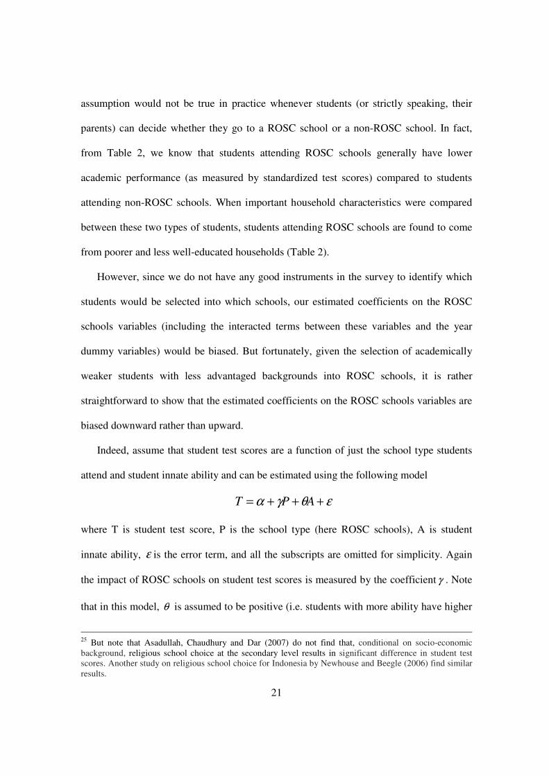
21

assumption would not be true in practice whenever students (or strictly speaking, their

parents) can decide whether they go to a ROSC school or a non-ROSC school. In fact,

from Table 2, we know that students attending ROSC schools generally have lower

academic performance (as measured by standardized test scores) compared to students

attending non-ROSC schools. When important household characteristics were compared

between these two types of students, students attending ROSC schools are found to come

from poorer and less well-educated households (Table 2).

However, since we do not have any good instruments in the survey to identify which

students would be selected into which schools, our estimated coefficients on the ROSC

schools variables (including the interacted terms between these variables and the year

dummy variables) would be biased. But fortunately, given the selection of academically

weaker students with less advantaged backgrounds into ROSC schools, it is rather

straightforward to show that the estimated coefficients on the ROSC schools variables are

biased downward rather than upward.

Indeed, assume that student test scores are a function of just the school type students

attend and student innate ability and can be estimated using the following model

εθγα +++= APT

where T is student test score, P is the school type (here ROSC schools), A is student

innate ability, ε is the error term, and all the subscripts are omitted for simplicity. Again

the impact of ROSC schools on student test scores is measured by the coefficient γ . Note

that in this model, θ is assumed to be positive (i.e. students with more ability have higher

25 But note that Asadullah, Chaudhury and Dar (2007) do not find that, conditional on socio-economic background, religious school choice at the secondary level results in significant difference in student test scores. Another study on religious school choice for Indonesia by Newhouse and Beegle (2006) find similar results.

22

test scores), and the correlation between P and A is negative or 0),cov( <AP (i.e.

academically weaker students are more likely to attend ROSC schools, which are shown

in Table 2). Since student innate ability is unobserved, and A cannot be included in the

regression, our estimate γ̂ of γ is biased, and it is in fact (Greene, 2008, p. 134)

.)var(

),cov(),|ˆ( θγγ

P

APAPE += Since ,0)var(,0),cov( >< PAP and 0>θ , the second term in

this expression is negative. Thus, our estimate γ̂ of γ is biased downward.

Thus, any estimated impacts of ROSC schools would represent the lower bounds of

the true impacts. And it is perhaps reasonable to make the second assumption with a

number of control variables on school characteristics that we use.

With some minor changes in notation, we can evaluate the impacts of ROSC schools

on student learning outcomes using a model which is similar to, although somewhat

simpler than, equation (1). However, the school (and student) questionnaires are slightly

different from the household questionnaires, thus the explanatory variables are slightly

different as described below. The model is an intention-to-treat (ITT) model and assumed

to be

istiis

K

kkk

K

kkkist Z YP YPT εµηγδβα ++++++= ∑∑

== 11* (2)

where the variables are defined as follows

α : constant term

istT : learning outcomes, as measured by standardized test scores, for child i in school s at

time t

23

kP : program school, with k= 1, 2. 1P being the Grant (G) schools and 2P being the

Grant+ Allowance (GA) schools. The reference category is the non-ROSC schools in non-

ROSC areas (pure control group).

Y : year dummy variable, which equals 1 for the year 2009 and 0 for the year 2006

isZ : other control variables including individual, household, and school characteristics

obtained from the follow-up survey.

Individual characteristics include student gender and age. Household characteristics

include parental literacy, household size, and household living standards as measured by a

housing asset index.26 School characteristics include the time it takes each student to get to

school, the frequency of homework assignment in English and Mathematics for each

student, the number of days the school was open in the last two weeks, the condition of

school classrooms, the condition of classroom blackboards, and school infrastructure such

as whether the school has a toilet, an alphabetic chart, a number chart, electricity or water.

The child random effects iµ , the random error term istε , and the within-individual

correlation ρ are defined in a similar way to equation (1).27 Also similar to equation (1),

standard errors are clustered at the individual level to address any possible heterogeneity

in the error terms.

Again, the most interesting coefficients in equation (2) are kγ , which are the

coefficients on the treatment variables YPk * obtained by interacting the program school

26 We use a housing asset index since the student questionnaire does not contain a household consumption module which can allow calculation of household expenditures. This asset index is the first principal component of household assets such as television, fan, bicycle, phone, and access to electricity. 27 Again, estimation results using a student fixed-effects model (not shown) are very similar to the random-effects model. Hausman tests do not reject the null of no difference between these two models, except for math scores. Furthermore, since all the time-invariant variables including student and school characteristics will be washed out in the student fixed-effects model, we prefer to use the random-effects model.

24

variables and the year variables. These coefficients represent the treatment impacts on test

scores in 2009 compared to 2006 for students attending different types of school. In other

words, these coefficients measure the relative gains in test scores for ROSC schools

compared to non-ROSC schools in non-ROSC areas (ITT sample) over time.

Estimation Results

Estimation results are provided in Table 5 for the impacts of ROSC schools (G schools

and GA schools) on test scores compared to non-ROSC schools. The coefficients on the

interacted terms between G schools and GA schools and the year dummy variable have

mixed signs, although they are mostly positive. However, these coefficients are small in

size and not statistically different from zero across all models. This implies that, both G

schools and GA schools have similar impacts on the gains in student test scores as non-

ROSC schools. In other words, during 2006- 2009, ROSC schools are performing as well

as non-ROSC schools in boosting student test scores.28

Given the lower starting points in test scores for students attending ROSC schools,

especially GA schools (Table 2), and that ROSC schools are much smaller and more

recently established than non-ROSC schools, this indicates perhaps no small achievement

of the ROSC project. In particular, as discussed above, since the true impacts of ROSC

schools are underestimated, these impacts are just conservative estimates.

28 It is interesting to see that there is not much difference between the impacts of G and GA schools on test scores, although G schools have somewhat stronger effects on enrolment as shown in the previous Section. We believe this can be explained by two main reasons. First, during the project implementation, G schools are also found to provide some allowances to students, thus effectively making them similar to GA schools. Second, there is evidence that allowances to students are not efficiently targeted toward the poorest through non-optimal project management which can contaminate the original project design. See Sarr et al. (2010) for more details and also the next footnote.

25

Other variables, except for student gender, have the expected impacts. Students

coming from wealthier households and/ or having literate parents have higher test scores.

The longer students live from school, the more likely they have lower test scores; however

this is mostly marginally significant at the 10 percent level. While the frequency of math

homework has no statistically significant impact on test scores, more English homework

can improve math test scores by 0.2 standard deviations, perhaps suggesting some

complementary impacts of verbal skills on math skills. School with better blackboards or

with number charts or with water has positive impacts on both Bangla and math test

scores. For example, a number chart can increase math scores by as much as 0.2 standard

deviations. But it is somewhat puzzling that alphabetic charts can somehow reduce student

math scores.

It is interesting to note in Table 5 that girls have around 0.1 standard deviations higher

gains in Bangla test scores than boys. However, girls do not have higher math scores than

boys. To further investigate these gender differences, we rerun the same regressions in

Table 5 separately for girls and boys and provide estimation results in Table 6. These

results show that in general there is no difference in the impacts of ROSC schools on test

scores for boys or girls, although girls studying at GA schools appear to have higher math

test scores (which are marginally significant at the 11 percent level).

Robustness Checks

Tests Taken at School versus at Home

As discussed in the previous section, around 70 percent of the children with both

baseline and follow-up test scores took the follow-up test at school, and the remaining

children took this test at home. It can be argued that the environment under which the test

26

was taken can affect student test scores in various ways (e.g. students may be more

focused at school or lighting conditions may be different between school and home). Thus

as robustness check, we drop all the children that took tests at home and rerun the

estimations in Table 5. Estimation results (not shown) indicate no difference from those in

Table 5, suggesting that our results are robust to the place where the tests were taken.

Student Transfer

Is it possible that parents may respond to the incentives offered in the ROSC schools

(e.g. student allowances at GA schools) by withdrawing their children from other schools

and enroll them in ROSC schools? Our calculation shows that around 30 percent of

children that were enrolled in ROSC schools had been enrolled in some other primary or

Madrasa schools before. In such cases, this can increase the test scores at ROSC schools

and bias our estimates upward if these students have better academic ability, and bias our

estimates downward vice versa. To check on this hypothesis, we drop all the children in

the estimation sample who had been attending non-ROSC schools before enrolling in

ROSC schools and re-run the estimation in Table 5. Estimation results (not shown here),

however, are not different from the previous results, thus indicate our results are robust to

including or excluding these transfer students who had been enrolled in non-ROSC

schools prior to attending ROSC schools.

Impact Heterogeneity for Student Ability

As shown in Figures 1 and 2 above, the gains in test scores appear to vary for students

with different baseline scores, especially in GA schools compared to non-ROSC schools.

27

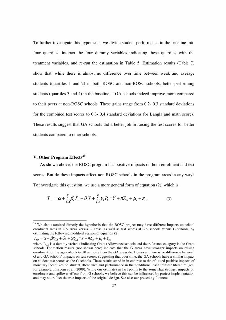
To further investigate this hypothesis, we divide student performance in the baseline into

four quartiles, interact the four dummy variables indicating these quartiles with the

treatment variables, and re-run the estimation in Table 5. Estimation results (Table 7)

show that, while there is almost no difference over time between weak and average

students (quartiles 1 and 2) in both ROSC and non-ROSC schools, better-performing

students (quartiles 3 and 4) in the baseline at GA schools indeed improve more compared

to their peers at non-ROSC schools. These gains range from 0.2- 0.3 standard deviations

for the combined test scores to 0.3- 0.4 standard deviations for Bangla and math scores.

These results suggest that GA schools did a better job in raising the test scores for better

students compared to other schools.

V. Other Program Effects29

As shown above, the ROSC program has positive impacts on both enrolment and test

scores. But do these impacts affect non-ROSC schools in the program areas in any way?

To investigate this question, we use a more general form of equation (2), which is

istiis

K

kkk

K

kkkist Z YP YPT εµηγδβα ++++++= ∑∑

== 11* (3)

29 We also examined directly the hypothesis that the ROSC project may have different impacts on school enrolment rates in GA areas versus G areas, as well as test scores at GA schools versus G schools, by estimating the following modified version of equation (2)

istiisGAGAist Z YP YPT εµηγδβα ++++++= *

where PGA is a dummy variable indicating Grant+Allowance schools and the reference category is the Grant schools. Estimation results (not shown here) indicate that the G areas have stronger impacts on raising enrolment for the age cohorts 6- 10 and 6- 8 than the GA areas do. However, there is no difference between G and GA schools’ impacts on test scores, suggesting that over time, the GA schools have a similar impact on student test scores as the G schools. These results stand in in contrast to the oft-cited positive impacts of monetary incentives on student attendance and performance in the conditional cash transfer literature (see, for example, Fiszbein et al., 2009). While our estimates in fact points to the somewhat stronger impacts on enrolment and spillover effects from G schools, we believe this can be influenced by project implementation and may not reflect the true impacts of the original design. See also our preceding footnote.

28

The variables are defined as in equation (2) above, except for the change to the variable kP

representing program schools, with k= 1, 2, 3, 4; 1P being the Grant (G) schools, 2P the

Grant+ Allowance (GA) schools, 3P non-ROSC schools in G areas, and 4P non-ROSC

schools in GA areas. The reference category is the non-ROSC schools in non-ROSC

areas.

Estimation results (Table 8) show that students attending non-ROSC schools in ROSC

areas generally improve their test scores more than students attending non-ROSC schools

in non-ROSC areas, with the improvement ranging from 0.3 standard deviations in math

scores to 0.53 standard deviations in Bangla scores and combined scores. In particular,

students attending non-ROSC schools in G areas gain more than those attending non-

ROSC schools in GA areas. The gains for the former group are from twice more than to

almost three times higher than those for the latter group.

There are two possible explanations for this difference. First, ROSC schools may have

done a good job in attracting both out-of-school children and the weaker students in

ROSC areas—who would have gone to non-ROSC school in ROSC areas in the absence

of ROSC schools—thus leaving non-ROSC schools in ROSC areas with better students.

This hypothesis appears to be consistent with the results in Table 3, where ROSC schools

are found to significantly raise school enrolment in ROSC areas. Second, the presence of

ROSC schools, especially G schools, may increase the efficiency for non-ROSC schools

in ROSC areas, perhaps most likely through increased competition for student enrolment.

This hypothesis would be consistent with Hoxby (2000, 2002)’s argument that public

schools are likely to respond to competition from choice schools (ROSC schools in our

case) by raising their student achievement.

29

At the same time, there is almost no change to the test scores for student attending

ROSC schools versus those attending non-ROSC schools in non-ROSC areas, which is

reassuring and confirms the robustness of the results discussed earlier in Table 5.

VI. Relative Efficiency of ROSC Schools

ROSC schools appear to operate more efficiently than government primary (GP)

schools in several aspects. 30 First, ROSC schools are organized around a single teacher in

one classroom, thus they exhibit low operating costs compared to GP schools. ROSC

schools often rent a room in a house to serve as a classroom in which multiple grades are

being taught by the same teacher.

Second, teacher salaries—which usually represent the lion’s share of operational

expenses for the education sector in developing countries—are also much smaller in

ROSC schools. While the average annual government expenditure per student at ROSC

schools is around Taka 1,489 (Sarr et al., 2010), the corresponding figure for GP schools

is more than twice higher at Taka 3,108 (GOB, 2009).31 Furthermore, the majority of

ROSC teachers (85%) earn a monthly salary less than Taka 1,200 and ROSC teachers’

monthly salaries are rarely higher than Taka 1,500 (ROSC Project Office Unit, 2009).

This monthly salary is more than six times less than the monthly salary of Taka 7,515 for

the least qualified teachers (who are assistant teachers without a Primary Training Institute

(PTI) certificate), and the monthly salary of Taka 7,950 for the average teachers with a

PTI certificate.

30 We do not have data on costs for other non-ROSC schools including Madrasa schools, but the majority (95% or more) of non-ROSC schools in our estimation samples are government primary schools. 31 These numbers are recurrent unit costs and the former figure is for 2009 and the latter for 2008.

30

Notably, while the student-teacher ratio in ROSC schools (35 students per teacher) is

smaller than the corresponding figure (52 students per teacher) for GP schools,32 this

difference is still disproportionate to the wide disparity in teacher salaries.

Third, compared to GP schools, the management of ROSC schools is more

decentralized with Community Management Centers (CMC) working closely with local

NGOs,33 thereby enhancing the accountability in school management. Low teacher

absenteeism—less than 5 percent—is another characteristic of ROSC schools (ROSC

Monitoring Report 2009). Among teachers present in school during the survey visit, over

80% were actually teaching.

At the same time, students attending ROSC schools have equally substantially

improved their performance in Bangla and Math tests as well as their peers at non-ROSC

schools, and academically stronger students at GA schools have even improved more.

This relatively good performance of ROSC schools despite their low operating costs

seems to suggest that they are more efficient compared to non ROSC schools.34

It may be useful to reflect on the driving factors behind this efficiency at ROSC

schools. Unsurprisingly, the advantages of ROSC schools are built upon the same

characteristics of its prototype—the successful BRAC school model. In addition to the

features discussed earlier (e.g., BRAC schools have smaller class sizes and more contact

hours), two features that are often missing in GP schools can be highlighted.

32 An obvious implication of this is that ROSC students are more likely to get more attention from their teacher than their peers in non-ROSC schools. However, while there is no ROSC (or BRAC) secondary school, it should be noted that in the Bangladeshi context, smaller class sizes at the secondary school level may not lead to higher test scores (Asadullah, 2005). 33 These NGOs assist the ROSC school in identifying out-of-school children and hard-to-reach children, ensuring their enrolment and attendance, and support CMCs in running the ROSC schools. 34 In fact, evidence elsewhere shows that other models of non-formal schools in Honduras, Ghana, and Mali are also more cost-effective than their public counterparts (DeStefano et al., 2006).

31

First, BRAC schools are built and continuously improved upon the principle of

“listening to the people” since BRAC itself is “constantly soliciting and acting on

feedback, criticism, and suggestions” (Ahmed and French, 2006). This spirit results in the

dynamism and flexibility behind the BRAC school model, which has now been adopted in

a number of countries in Africa and Asia including Afghanistan, Liberia, Pakistan,

Tanzania, Southern Sudan, and Sri Lanka. In fact, the non-formal primary education

program is just an area among several others such as silk worms, microfinance, solar

panels, maternal health, recycled paper, and high fashion in which BRAC operates

projects based on a social entrepreneurship approach (BRAC, 2009). ROSC schools

understandably inherit this dynamism through a highly decentralized system with strong

community participation in management.

Second, the quality of teachers at BRAC schools is perceived to be higher than that of

their GP counterparts in several ways.35 Firstly, BRAC teachers are recruited from the

same local community as their students and have a close relationship with their students,

who they are responsible for during the full three-year (or four- year) cycles. In contrast to

GP teachers who may either neglect or resort to corporal punishment for their students,

BRAC teachers are affectionate to their students (Chabbot, 2006). Secondly, although

BRAC teachers’ formal education levels are often limited to high-school level (i.e., nine

or ten years of schooling) and lower than those of GP teachers, their skills are constantly

developed through needs-based and practical refresher training which occurs monthly.36 In

35 While raising a number of issues about the effectiveness of school resources, Hanushek strongly advocates the role of teacher quality in raising educational outcomes. See, for example, Hanushek (2011) and Hanushek and Rivkin (2006). 36 It is interesting to note that recent evidence for the US suggests that neither holding a college major in education nor more advanced degree is associated with elementary and middle school teaching effectiveness (Chingos and Peterson, 2011).

32

addition, BRAC teachers also have much stronger support and supervision than their GP

counterparts (Haiplik, 2004). And thirdly, BRAC teachers are highly motivated, perhaps

not least because of the enhanced respect and standing in their communities obtained by

their teaching status.

VII. Conclusion

In this paper we investigate the impacts of ROSC schools versus other types of

schools on student enrolment and test score gains over time. This is a unique program

where the GOB for the first time experimented with bringing into the public system the

well-known NGO-run BRAC school model. We found that ROSC schools increase

enrolment probability between 9 and 18 percent and perform as well as non-ROSC

schools in raising test scores. In particular, better performing students attending GA

schools improve their test scores by around 0.2- 0.4 standard deviations compared to other

schools.

Furthermore, ROSC schools appear to have positive externalities on test scores for

students attending non-ROSC schools in program areas. These findings are robust to

different model assumptions and specifications. Given the selection of academically

weaker students coming from less advantaged households into ROSC schools, we also

show that our estimated impacts are conservative (i.e., biased downward). Notably,

despite this impressive performance ROSC schools, among other things, have much lower

operational costs than GP schools.

Given mixed results about the effects of different components of school resources,

these results about the positive impacts of ROSC schools appear quite encouraging. While

future research may focus on disentangling and quantifying further the particular

33

characteristics that make ROSC (or BRAC) schools stand out from other school models,

our results point to the effectiveness of this non-formal school model as a comprehensive

“package”, whose salient characteristics include streamlined operations, high teacher

quality, and a spirit of constant self-learning and self-improving.

Both the effectiveness and efficiency of the ROSC school program render it as an

attractive approach to increase schooling quantity and quality, especially as the GOB

plans to achieve the MDG goals of universal primary education by 2015. Our results

suggest that the ROSC program can be expanded on a larger scale in Bangladesh. We also

believe that these findings provide useful input for policy makers in Bangladesh and other

countries that may plan to adopt a similar schooling model.

34

References

Ahmed, Akhter U. (2006). “Evaluating the Reaching Out Of School Children Project in

Bangladesh: A Baseline Study.” International Food Policy Research Institute, IFPRI,

Washington, DC.

Ahmed, Manzoor. (2008). “Policy Options in Non-Formal Education”. In William K.

Cummings and James H. Williams. (Eds). “Policy-Making in Education Reforms in

Developing Countries: Policy Options and Strategies”. Rowman & Littlefield

Education: United States of America.

Ahmed, Salehuddin and Micaela French. (2006). “Scaling Up- The BRAC Experience”.

BRAC University Journal, 3(2): 35-40.

Arif, G. M. and Najam Us Saqib. (2003), “Production of Cognitive and Life Skills in

Public, Private, and NGO Schools in Pakistan”. Pakistan Development Review. 42: 1

(Spring 2003) pp. 1–28.

Asadullah, Mohammad Niaz. (2005). “The Effect of Class Size on Student Achievement:

Evidence from Bangladesh”. Applied Economics Letter, 12: 217- 221.

Asadullah, Mohammad Niaz, Nazmul Chaudhury, and Amit Dar. (2007). “Student

Achievement Conditioned upon School Selection: Religious and Secular Secondary

School Quality in Bangladesh.” Economics of Education Review 26(6): 648–59.

Banerjee, Abhijit V., Shawn Cole, Esther Duflo, and Leigh Linden. (2007). “Remedying

Education: Evidence from Two Randomized Experiments in India.” Quarterly Journal

of Economics 122 (3): 1235–64.

Banerjee, Abhijit V., Rukmini Banerji, Esther Duflo, Rachel Glennerster, and Stuti

Khemani. (2010). “Pitfalls of Participatory Programs: Evidence from a Randomized

Evaluation in Education in India”. American Economic Journal: Economic Policy,

2:1, 1–30.

Becker, Gary, and H. G. Lewis. (1973). “On the Interaction between the Quantity and

Quality of Children.” Journal of Political Economy 81: S279-288.

BRAC (Bangladesh Rural Advancement Committee). (2009). “BRAC Annual Report

2009”. Available on the Internet at http://www.brac.net/oldsite/useruploads/files/brac-

ar-2009.pdf. (Accessed in March 2011).

35

Chabbot, Colette. (2006). “Meeting EFA: Bangladesh Rural Advancement Committee

(BRAC) Primary Schools”. Washington DC: Academy for Education Development.

www.equip123.net

Chingos, Mathew M. and Paul E. Peterson. (2011). “It’s Easier to Pick a Good Teacher

Than to Train One: Familiar and New Results on the Correlates of Teacher

Effectiveness.” Economics of Education Review, 30: 449-465.

Dang, Hai-Anh, and Halsey Rogers. (2008). “The Growing Phenomenon of Private

Tutoring: Does It Deepen Human Capital, Widen Inequalities, or Waste Resources?”

World Bank Research Observer 23(2): 161-200.

Data Analysis and Technical Analysis (DATA). (2010). “Public Expenditure Tracking

Survey and Impact Evaluation for Reaching Out Of School Children Project (ROSC)

Follow-up Survey Report”. Dhaka, Bangladesh.

DeStefano, Joseph, Ash Hartwell, Audrey-marie Schuh Moore, and Jen Benbow. (2006).

“A Cross-National Cost-Benefit Analysis of Complementary (Out-Of-School)

Programs”. Journal of International Cooperation in Education, 9(1): 71- 88.

Duflo, Esther, Pascaline Dupas, and Michael Kremer. 2010. “Pupil-Teacher Ratio,

Teacher Management and Education Quality: Experimental Evidence from Kenyan

Primary Schools”. Mimeo, MIT.

Evans, David, Michael Kremer, and Muthoni Ngatia. (2008). “The Impact of Distributing

School Uniforms on Children’s Education in Kenya.” Working paper, Harvard

University.

Farrell, Joseph P. (2004). “The Egyptian Community Schools Program: A Case Study”.

Washington DC: Academy for Education Development. www.equip123.net

Farrell, Joseph P. and Ash Hartwell. (2008). “Planning for Successful Alternative

Schooling: A Possible Route to Education for All”. International Institute for

Education Planning research paper.

Filmer, Deon. (2007). "If You Build It, Will They Come? School Availability and School

Enrolment in 21 Poor Countries." Journal of Development Studies, 43(5): 901-928.

Fiszbein, Ariel, Norbert Schady, Francisco H. G. Ferreira, Margaret Grosh, Nial Kelleher,

Pedro Olinto, and Emmanuel Skoufias. (2009). "Conditional Cash Transfers:

Reducing Present and Future Poverty." World Bank. Washington DC: USA.

36

Glewwe, Paul, Michael Kremer, Sylvie Moulin, and Eric Zitzewitz. (2004).

“Retrospective vs. Prospective Analyses of School Inputs: The Case of Flip Charts in

Kenya”. Journal of Development Economics, 74: 251- 268.

Glewwe, Paul, and Michael Kremer. (2006). “School, Teachers, and Education Outcomes

in Developing Countries.” In Eric A. Hanushek and Finis Welch, eds., Handbook of

the Economics of Education. Amsterdam: North-Holland.

Glewwe, Paul, Michael Kremer, and Sylvie Moulin. (2009). “Many Children Left

Behind? Textbooks and Test Scores in Kenya”. American Economic Journal: Applied

Economics 2009, 1:1, 112–135

Glewwe, Paul, Nauman Ilias, and Michael Kremer. (2010). “Teacher Incentives”.

American Economic Journal: Applied Economics 2 (July 2010): 205–227.

Government of Bangladesh (GOB), General Economic Division, Planning Commission.

(2009). “Millennium Development Goals Needs Assessment and Costing 2009- 2015

Bangladesh”. Available on the Internet at

http://www.undp.org.bd/info/pub/MDG%20Needs%20Assessment%20&%20Costing

%202009-2015%20small.pdf (accessed in February 2011).

Haiplik, Brenda Mary. (2004). “An Educational Success Story from Bangladesh:

Understanding the BRAC Non-Formal Primary Education Model and Its Teacher

Training and Development System”. Unpublished Ph.D. thesis, University of Toronto.

Hanushek, Erik A. (2006). “School Resources”. In Eric A. Hanushek and Finis Welch,

eds., Handbook of the Economics of Education. Amsterdam: North-Holland.

---. (2011). “The Economic Value of Higher Teacher Quality”. Economics of Education

Review, 30: 466-479.

Hanushek, Erik A. and Steven G. Rivkin. (2006). “Teacher Quality”. In Eric A. Hanushek

and Finis Welch, eds., Handbook of the Economics of Education. Amsterdam: North-

Holland.

Hartwell, Ash. (2006). “Meeting EFA: Ghana School for Life”. Washington DC:

Academy for Education Development. www.equip123.net

Hoxby, Caroline. (2000). “Does Competition Among Public Schools Benefit Students and

Tax Payers?” American Economic Review, 90(5): 1209-1238.

---. (2002). “How School Choice Affects Public School Students’ Achievement”. In

Paul Hill, eds. Choice with Equity. Stanford: Hoover Institution Press.

37

Kremer, Michael and Alaka Holla. (2009). “Improving Education in the Developing

World: What Have We Learned from Randomized Evaluations?” Annual Review of

Economics, 1: 513-542.

Kremer, Michael, Edward Miguel, and Rebecca Thornton. (2009). “Incentives to Learn,”

Review of Economics and Statistics, 91(3): 437-456.

Khan, S.R. and Kiefer, D. (2007) “Educational Production Functions for Rural Pakistan:

A Comparative Institutional Analysis”, Education Economics, 15 (3): 327-342.

Greene, William. (2008). “Econometric Analysis, 6th Edition”. New Jersey: Prentice Hall.

McEwan, Patrick. (1998). “The Effectiveness of Multigrade Schools in Columbia”.

International Journal of Educational Development, 18(6): 435-452.

Muralidharan, Karthik and Venkatesh Sundararaman. (2009). “Teacher Performance Pay:

Experimental Evidence from India”. National Bureau of Economic Research Working

Paper #15323.

Newhouse, David and Kathleen Beegle. (2006). “The Effect of School Type on Academic

Achievement: Evidence from Indonesia.” Journal of Human Resources 41(3): 529–57.

Psacharopolous, George, Carlos Rojas, and Eduardo Velez. (1993). “Achievement

Evaluation of Colombia's" Escuela Nueva": Is Multigrade the Answer?”. Comparative

Education Review, 37(3): 263- 276.

Sarr, Leopold Remi, Hai-Anh Dang, Nazmul Chaudhury, Dilip Parajuli, and Niaz

Asadullah. (2010). “Reaching Out of Children Project Evaluation Report”. South

Asian Human Development Sector, World Bank.

ROSC Project Office Unit. (2009). “ROSC Monitoring Cell Report”. Dhaka, Bangladesh.

Sud, Pamela. (2010) “Can Non-formal Education Keep Working Children in School? A

Case Study from Punjab, India”, Journal of Education and Work, 23(1): 1 – 26.

Sukontamarn, Pataporn. (2006). “The Entry of NGO Schools and Girls’ Educational

Outcomes in Bangladesh”. Working paper, University of Adelaide.

World Bank. (2011). World Development Indicators Online. Available on the Internet at

http://data.worldbank.org/indicator/PA.NUS.FCRF (accessed February 2011).

38

Figure 1: Distribution of Standardized Test Scores, Bangladesh 2006- 2009

0.2

.4.6

De

nsity

-2 -1 0 1 2Test scores in 2006

std. test scores for G schools

std. test scores for GA schools

std. test scores for control schools

0.2

.4.6

De

nsity

-2 -1 0 1 2Test scores in 2009

std. test scores for G schools

std. test scores for GA schools

std. test scores for control schools

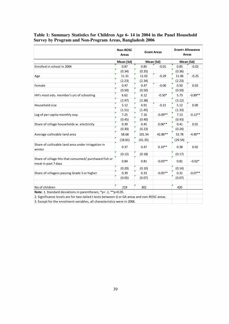
39

Table 1: Summary Statistics for Children Age 6- 14 in 2004 in the Panel Household

Survey by Program and Non-Program Areas, Bangladesh 2006

Non-ROSC

Areas

Mean (Sd)

Enrolled in school in 2004 0.87 0.85 -0.01 0.85 -0.02

(0.34) (0.35) (0.36)

Age 11.31 11.02 -0.29 11.06 -0.25

(2.23) (2.34) (2.23)

Female 0.47 0.47 -0.00 0.50 0.03

(0.50) (0.50) (0.50)

HH's most edu. member's yrs of schooling 6.62 6.12 -0.50* 5.73 -0.89**

(2.97) (3.38) (3.12)

Household size 5.12 4.91 -0.21 5.12 0.00

(1.51) (1.45) (1.33)

Log of per capita monthly exp. 7.25 7.16 -0.09** 7.13 -0.12**

(0.45) (0.40) (0.43)

Share of village households w. electricity 0.39 0.45 0.06** 0.41 0.01

(0.30) (0.23) (0.24)

Average cultivable land area 58.68 101.54 42.86** 53.78 -4.90**

(18.81) (41.35) (29.54)

Share of cultivable land area under irriagation in

winter0.37 0.47 0.10** 0.38 0.02

(0.12) (0.18) (0.17)

Share of village hhs that consumed/ purchased fish or

meat in past 7 days0.84 0.81 -0.03** 0.81 -0.02*

(0.20) (0.10) (0.14)

Share of villagers passing Grade 5 or higher 0.39 0.33 -0.05** 0.31 -0.07**

(0.05) (0.07) (0.07)

No of children 219 302 420

Note: 1. Standard deviations in parentheses; *p< .1, **p<0.05.

2. Significance levels are for two-tailed t tests between G or GA areas and non-ROSC areas.

3. Except for the enrolment variables, all characteristics were in 2006.

Grant AreasGrant+ Allowance

Areas

Mean (Sd) Mean (Sd)

40

Table 2: Summary Statistics for Children with Test Scores by Program and Non-

Program Schools, Bangladesh 2009

Non-ROSC Schools

in Non-ROSC areas

Mean (Sd) Mean (Sd) Dif. Mean (Sd) Dif.

Bangla Scores in 2006 (percent) 55.94 52.92 -3.02 33.27 -22.67**

(33.28) (36.42) (37.10)

Math Scores in 2006 (percent) 55.30 54.56 -0.74 43.54 -11.76**

(32.69) (34.34) (39.03)

Combined Scores in 2006 (percent) 55.70 53.53 -2.17 37.12 -18.58**

(27.34) (30.04) (33.63)

Age 10.87 11.67 0.80* 11.57 0.70

(6.07) (3.51) (5.78)

Female 0.53 0.45 -0.08** 0.49 -0.04

(0.50) (0.50) (0.50)

Household asset index 0.60 0.17 -0.43** -0.46 -1.06**

(1.66) (1.71) (1.39)

Literate parent(s) 0.70 0.51 -0.19** 0.53 -0.17**

(0.46) (0.50) (0.50)

Female head 0.10 0.09 -0.01 0.09 -0.01

(0.30) (0.28) (0.28)

Household size 4.89 4.82 -0.07 5.09 0.2

(1.51) (1.43) (2.13)

Time to school 12.79 7.74 -5.05** 6.21 -6.58**

(10.07) (6.53) (6.24)

English homework most of the week 0.97 0.92 -0.05** 0.76 -0.21**

(0.16) (0.27) (0.43)

Math homework most of the week 0.96 0.95 -0.01 0.77 -0.19**

(0.19) (0.22) (0.42)

No of days school open last 2 weeks 11.08 11.33 0.25** 10.03 -1.05**

(1.43) (1.81) (2.36)

Condition of blackboard 3.00 2.87 -0.13** 2.78 -0.22**

(0.00) (0.44) (0.64)

School has toilet 0.93 0.54 -0.39** 0.32 -0.61**

(0.25) (0.50) (0.47)

School has alphabetic chart 0.54 0.34 -0.2** 0.27 -0.27**

(0.50) (0.47) (0.45)

School has number chart 0.54 0.15 -0.39** 0.19 -0.35**

(0.50) (0.36) (0.39)

School has electricity 0.67 0.10 -0.57** 0.12 -0.55**

(0.47) (0.30) (0.32)

School has water 0.94 0.76 -0.18** 0.41 -0.53**

(0.24) (0.43) (0.49)

No of children 217 833 782

Note: 1. Standard deviations in parentheses. The differences are between program schools and control schools.

2. Significance levels are for two-tailed t tests with unequal variances between G or GA schools and

non-ROSC schools; *p< .1, **p<0.05.

3. Except for the test scores, all characteristics were in 2009.

G Schools GA Schools

41

Table 3: Impacts of ROSC Project on School Enrolment, Bangladesh 2009

Model 1 Model 2 Model 3 Model 4 Model 5 Model 6 Model 7 Model 8 Model 9

G areas* 2006 0.117*** 0.121*** 0.121*** 0.188*** 0.191*** 0.191*** 0.012 0.016 0.016

(0.043) (0.043) (0.043) (0.056) (0.056) (0.056) (0.034) (0.034) (0.034)

GA areas* 2006 0.089** 0.092** 0.092** 0.118** 0.121** 0.121** 0.042 0.044 0.044

(0.037) (0.037) (0.037) (0.048) (0.048) (0.048) (0.029) (0.029) (0.029)

G areas* 2007 0.071 0.075 0.074 0.165*** 0.164*** 0.161*** -0.031 -0.023 -0.024

(0.051) (0.051) (0.051) (0.062) (0.062) (0.062) (0.043) (0.042) (0.043)

GA areas* 2007 0.021 0.026 0.017 0.089 0.089 0.076 -0.019 -0.018 -0.024

(0.046) (0.046) (0.047) (0.056) (0.056) (0.057) (0.038) (0.038) (0.038)

G areas* 2008 0.117** 0.120** 0.120** 0.179*** 0.178*** 0.175*** 0.020 0.028 0.027

(0.055) (0.055) (0.055) (0.066) (0.066) (0.066) (0.047) (0.046) (0.047)

GA areas* 2008 0.013 0.018 0.010 0.060 0.060 0.047 -0.025 -0.024 -0.030

(0.051) (0.051) (0.052) (0.061) (0.061) (0.062) (0.043) (0.042) (0.042)

G areas -0.145*** -0.128*** -0.118** -0.215*** -0.194*** -0.189*** -0.042 -0.021 0.013

(0.045) (0.043) (0.049) (0.059) (0.055) (0.062) (0.035) (0.034) (0.041)

GA areas -0.098** -0.077** -0.061 -0.112** -0.097* -0.073 -0.067** -0.034 -0.016

(0.040) (0.039) (0.042) (0.053) (0.050) (0.054) (0.033) (0.031) (0.034)

Year 2006 0.097*** 0.094*** 0.094*** 0.133*** 0.130*** 0.130*** -0.002 -0.005 -0.005

(0.027) (0.027) (0.027) (0.035) (0.035) (0.035) (0.021) (0.021) (0.021)

Year 2007 0.077** 0.057 0.054 0.122*** 0.111** 0.112** -0.059** -0.093*** -0.100***

(0.035) (0.036) (0.036) (0.043) (0.044) (0.043) (0.029) (0.029) (0.029)

Year 2008 0.008 -0.012 -0.015 0.081* 0.069 0.070 -0.142*** -0.176*** -0.183***

(0.039) (0.040) (0.040) (0.047) (0.047) (0.047) (0.033) (0.033) (0.034)

Age 0.324*** 0.324*** 0.565 0.639 0.087 0.084

(0.107) (0.108) (0.421) (0.432) (0.069) (0.069)

Age squared -0.017*** -0.017*** -0.030 -0.034 -0.006** -0.006**

(0.005) (0.005) (0.023) (0.024) (0.003) (0.003)

Female 0.107*** 0.107*** 0.096*** 0.096*** 0.100*** 0.100***

(0.018) (0.018) (0.021) (0.021) (0.020) (0.020)

HH's most edu. member's yrs of

schooling0.023*** 0.023*** 0.021*** 0.021*** 0.038*** 0.038***

(0.003) (0.003) (0.004) (0.004) (0.004) (0.004)

Household size -0.028*** -0.028*** -0.031*** -0.030*** -0.019*** -0.019***

(0.007) (0.007) (0.008) (0.008) (0.007) (0.007)

Log of per capita monthly exp. 0.090*** 0.087*** 0.082*** 0.079** 0.120*** 0.115***

(0.025) (0.026) (0.030) (0.031) (0.028) (0.029)

Share of village households w.

electricity-0.085 -0.067 -0.088

(0.055) (0.064) (0.058)

Average cultivable land area 0.000 0.000 -0.000

(0.000) (0.000) (0.000)

Share of cultivable land area

under irriagation in winter0.036 -0.002 0.056

(0.071) (0.081) (0.075)

Share of village hhs that

consumed/ purchased fish or

meat in past 7 days

0.157* 0.133 0.159*

(0.084) (0.098) (0.084)

Share of villagers passing Grade

5 or higher0.173 0.274 0.214

(0.215) (0.247) (0.225)

Constant 0.841*** -1.394** -1.550*** 0.805*** -2.429 -2.945 0.862*** -0.330 -0.453

(0.031) (0.561) (0.565) (0.042) (1.890) (1.953) (0.025) (0.456) (0.457)

R2 0.04 0.13 0.14 0.08 0.17 0.18 0.03 0.22 0.22

ρ 0.34*** 0.27*** 0.27*** 0.31*** 0.25*** 0.25*** 0.54*** 0.44*** 0.44***

No of children 661 661 661 440 440 440 799 799 799

Total no of obs. 2620 2620 2620 1748 1748 1748 3164 3164 3164

Note: 1. *p< .1, **p<0.05, ***p<0.01; robust standard errors in parentheses accounts for clustering at the child level.

2. All regressions control for child random effects.

Age 6- 10 in 2004 Age 6- 8 in 2004 Age 7- 14 in 2004

42

Table 4: Impacts of ROSC Project on School Enrolment for Boys and Girls, Bangladesh 2009

Model 1 Model 2 Model 3 Model 4 Model 5 Model 6 Model 7 Model 8 Model 9

A. Boys

G areas* 2006 0.078 0.083 0.083 0.154* 0.157* 0.157* 0.008 0.011 0.011

(0.063) (0.063) (0.063) (0.081) (0.081) (0.081) (0.043) (0.043) (0.043)

GA areas* 2006 0.068 0.071 0.070 0.083 0.086 0.086 0.015 0.017 0.017

(0.057) (0.058) (0.058) (0.073) (0.073) (0.073) (0.039) (0.039) (0.039)

G areas* 2007 0.054 0.065 0.075 0.163* 0.166* 0.172* -0.030 -0.018 -0.016

(0.076) (0.075) (0.076) (0.090) (0.088) (0.088) (0.059) (0.058) (0.059)

GA areas* 2007 0.005 0.014 0.011 0.069 0.070 0.057 -0.039 -0.037 -0.035

(0.071) (0.072) (0.073) (0.085) (0.084) (0.086) (0.053) (0.054) (0.054)

G areas* 2008 0.136* 0.148* 0.157** 0.207** 0.209** 0.215** 0.043 0.055 0.057

(0.078) (0.077) (0.078) (0.092) (0.090) (0.091) (0.064) (0.063) (0.064)

GA areas* 2008 0.004 0.012 0.009 0.026 0.027 0.014 -0.030 -0.029 -0.026

(0.077) (0.077) (0.078) (0.093) (0.092) (0.094) (0.060) (0.059) (0.060)

Control variables

Individual &

householdsN Y Y N Y Y N Y Y

Schools N N Y N N Y N N Y

R2 0.04 0.15 0.16 0.07 0.19 0.20 0.03 0.20 0.20

ρ 0.41*** 0.35*** 0.35*** 0.39*** 0.33*** 0.33*** 0.61*** 0.54*** 0.54***

No of children 334 334 334 219 219 219 424 424 424

Total no of obs. 1326 1326 1326 873 873 873 1677 1677 1677

B. Girls

G areas* 2006 0.160*** 0.165*** 0.167*** 0.232*** 0.234*** 0.237*** 0.019 0.023 0.024

(0.057) (0.057) (0.057) (0.075) (0.075) (0.075) (0.054) (0.054) (0.054)

GA areas* 2006 0.114** 0.118*** 0.119*** 0.165*** 0.167*** 0.169*** 0.071* 0.075* 0.075*

(0.046) (0.046) (0.046) (0.061) (0.061) (0.061) (0.042) (0.043) (0.043)

G areas* 2007 0.091 0.093 0.087 0.162* 0.160* 0.154* -0.031 -0.025 -0.026

(0.068) (0.068) (0.068) (0.085) (0.085) (0.085) (0.063) (0.062) (0.062)

GA areas* 2007 0.030 0.034 0.024 0.096 0.095 0.084 0.004 0.005 -0.009

(0.057) (0.057) (0.058) (0.072) (0.072) (0.073) (0.053) (0.052) (0.053)

G areas* 2008 0.095 0.097 0.091 0.143 0.140 0.135 -0.007 -0.001 -0.002

(0.077) (0.077) (0.077) (0.095) (0.095) (0.095) (0.070) (0.069) (0.069)

GA areas* 2008 0.012 0.015 0.005 0.073 0.072 0.061 -0.020 -0.019 -0.032

(0.067) (0.067) (0.068) (0.080) (0.080) (0.080) (0.061) (0.060) (0.060)

Control variables

Individual &

householdsN Y Y N Y Y N Y Y

Schools N N Y N N Y N N Y

R2 0.06 0.10 0.11 0.12 0.16 0.17 0.04 0.22 0.23

ρ 0.17*** 0.14*** 0.14*** 0.15*** 0.11*** 0.11*** 0.41*** 0.28*** 0.28***

No of children 327 327 327 221 221 221 375 375 375

Total no of obs. 1294 1294 1294 875 875 875 1487 1487 1487

Note: 1. *p< .1, **p<0.05, ***p<0.01; robust standard errors in parentheses accounts for clustering at the child level.

2. All regressions control for child random effects.

3. The control variables for the regressions are the same as those in Table 3.

Age 6- 10 in 2004 Age 6- 8 in 2004 Age 7- 14 in 2004

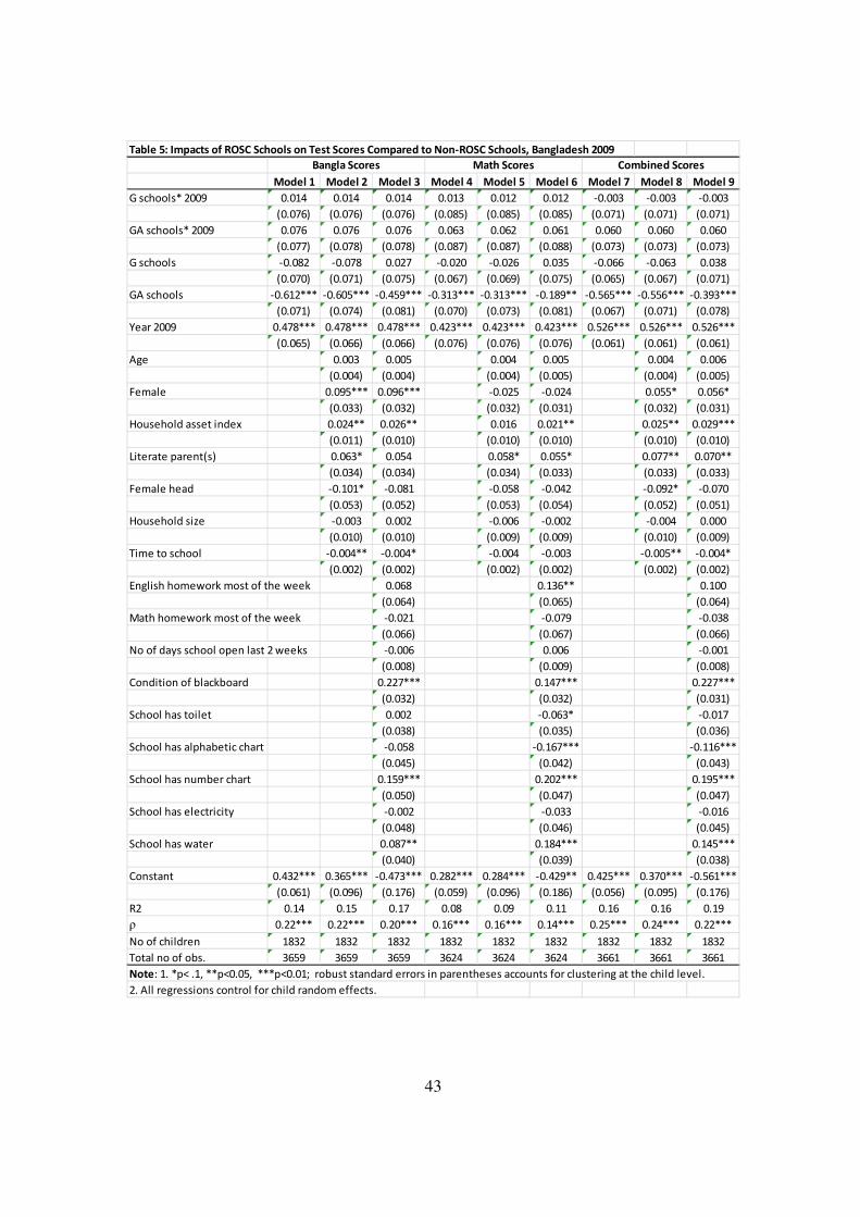
43

Table 5: Impacts of ROSC Schools on Test Scores Compared to Non-ROSC Schools, Bangladesh 2009

Model 1 Model 2 Model 3 Model 4 Model 5 Model 6 Model 7 Model 8 Model 9

G schools* 2009 0.014 0.014 0.014 0.013 0.012 0.012 -0.003 -0.003 -0.003

(0.076) (0.076) (0.076) (0.085) (0.085) (0.085) (0.071) (0.071) (0.071)

GA schools* 2009 0.076 0.076 0.076 0.063 0.062 0.061 0.060 0.060 0.060

(0.077) (0.078) (0.078) (0.087) (0.087) (0.088) (0.073) (0.073) (0.073)

G schools -0.082 -0.078 0.027 -0.020 -0.026 0.035 -0.066 -0.063 0.038

(0.070) (0.071) (0.075) (0.067) (0.069) (0.075) (0.065) (0.067) (0.071)

GA schools -0.612*** -0.605*** -0.459*** -0.313*** -0.313*** -0.189** -0.565*** -0.556*** -0.393***

(0.071) (0.074) (0.081) (0.070) (0.073) (0.081) (0.067) (0.071) (0.078)

Year 2009 0.478*** 0.478*** 0.478*** 0.423*** 0.423*** 0.423*** 0.526*** 0.526*** 0.526***

(0.065) (0.066) (0.066) (0.076) (0.076) (0.076) (0.061) (0.061) (0.061)

Age 0.003 0.005 0.004 0.005 0.004 0.006

(0.004) (0.004) (0.004) (0.005) (0.004) (0.005)

Female 0.095*** 0.096*** -0.025 -0.024 0.055* 0.056*

(0.033) (0.032) (0.032) (0.031) (0.032) (0.031)

Household asset index 0.024** 0.026** 0.016 0.021** 0.025** 0.029***

(0.011) (0.010) (0.010) (0.010) (0.010) (0.010)

Literate parent(s) 0.063* 0.054 0.058* 0.055* 0.077** 0.070**

(0.034) (0.034) (0.034) (0.033) (0.033) (0.033)

Female head -0.101* -0.081 -0.058 -0.042 -0.092* -0.070

(0.053) (0.052) (0.053) (0.054) (0.052) (0.051)

Household size -0.003 0.002 -0.006 -0.002 -0.004 0.000

(0.010) (0.010) (0.009) (0.009) (0.010) (0.009)

Time to school -0.004** -0.004* -0.004 -0.003 -0.005** -0.004*

(0.002) (0.002) (0.002) (0.002) (0.002) (0.002)

English homework most of the week 0.068 0.136** 0.100

(0.064) (0.065) (0.064)

Math homework most of the week -0.021 -0.079 -0.038

(0.066) (0.067) (0.066)

No of days school open last 2 weeks -0.006 0.006 -0.001

(0.008) (0.009) (0.008)

Condition of blackboard 0.227*** 0.147*** 0.227***

(0.032) (0.032) (0.031)

School has toilet 0.002 -0.063* -0.017

(0.038) (0.035) (0.036)

School has alphabetic chart -0.058 -0.167*** -0.116***

(0.045) (0.042) (0.043)

School has number chart 0.159*** 0.202*** 0.195***

(0.050) (0.047) (0.047)

School has electricity -0.002 -0.033 -0.016

(0.048) (0.046) (0.045)

School has water 0.087** 0.184*** 0.145***

(0.040) (0.039) (0.038)

Constant 0.432*** 0.365*** -0.473*** 0.282*** 0.284*** -0.429** 0.425*** 0.370*** -0.561***

(0.061) (0.096) (0.176) (0.059) (0.096) (0.186) (0.056) (0.095) (0.176)

R2 0.14 0.15 0.17 0.08 0.09 0.11 0.16 0.16 0.19

ρ 0.22*** 0.22*** 0.20*** 0.16*** 0.16*** 0.14*** 0.25*** 0.24*** 0.22***

No of children 1832 1832 1832 1832 1832 1832 1832 1832 1832

Total no of obs. 3659 3659 3659 3624 3624 3624 3661 3661 3661

Note: 1. *p< .1, **p<0.05, ***p<0.01; robust standard errors in parentheses accounts for clustering at the child level.

2. All regressions control for child random effects.

Bangla Scores Math Scores Combined Scores

44

Table 6 :Impacts of ROSC Schools on Test Scores for Boys and Girls, Bangladesh 2009

Model 1 Model 2 Model 3 Model 4 Model 5 Model 6 Model 7 Model 8 Model 9

A. Boys

G schools* 2009 -0.003 -0.003 -0.003 -0.113 -0.113 -0.114 -0.071 -0.071 -0.071

(0.106) (0.106) (0.106) (0.122) (0.122) (0.123) (0.098) (0.098) (0.098)

GA schools* 2009 0.135 0.135 0.136 -0.088 -0.088 -0.091 0.036 0.036 0.036

(0.108) (0.108) (0.108) (0.127) (0.127) (0.127) (0.101) (0.101) (0.101)

Control variables

Individual &

householdsN Y Y N Y Y N Y Y

Schools N N Y N N Y N N Y

R2 0.17 0.19 0.21 0.10 0.10 0.13 0.19 0.20 0.23

ρ 0.21*** 0.20*** 0.19*** 0.13*** 0.13*** 0.10*** 0.23*** 0.22*** 0.19***

No of children 965 965 965 965 965 965 965 965 965

Total no of obs. 1926 1926 1926 1910 1910 1910 1928 1928 1928

B. Girls

G schools* 2009 0.019 0.019 0.019 0.114 0.114 0.114 0.046 0.046 0.046

(0.108) (0.108) (0.108) (0.119) (0.119) (0.119) (0.101) (0.101) (0.101)

GA schools* 2009 0.006 0.006 0.006 0.194 0.194 0.193 0.067 0.067 0.067

(0.111) (0.111) (0.111) (0.120) (0.120) (0.120) (0.104) (0.104) (0.105)

Control variables

Individual &

householdsN Y Y N Y Y N Y Y

Schools N N Y N N Y N N Y

R2 0.12 0.12 0.16 0.07 0.07 0.10 0.12 0.13 0.17

ρ 0.23*** 0.23*** 0.20*** 0.19*** 0.19*** 0.18*** 0.26*** 0.26*** 0.23***

No of children 867 867 867 867 867 867 867 867 867

Total no of obs. 1733 1733 1733 1714 1714 1714 1733 1733 1733

Note: 1. *p< .1, **p<0.05, ***p<0.01; robust standard errors in parentheses accounts for clustering at the child level.

2. All regressions control for child random effects.

3. The control variables for the regressions are the same as those in Table 5.

Bangla Scores Math Scores Combined Scores

45

Table 7: Robustness Checks on Impacts of ROSC Schools on Test Scores, Bangladesh 2009

Model 1 Model 2 Model 3 Model 4 Model 5 Model 6 Model 7 Model 8 Model 9

Quartile 1* G schools* 2009 -0.083 -0.072 -0.074 -0.041 -0.038 -0.036 -0.165* -0.154 -0.158*

(0.095) (0.095) (0.096) (0.108) (0.108) (0.108) (0.094) (0.095) (0.094)

Quartile 2* G schools* 2009 -0.004 0.010 0.004 0.009 0.012 -0.005 0.023 0.029 0.010

(0.093) (0.094) (0.094) (0.094) (0.094) (0.095) (0.083) (0.083) (0.083)

Quartile 3* G schools* 2009 0.029 0.026 0.022 0.041 0.038 0.046 0.025 0.021 0.023

(0.083) (0.083) (0.083) (0.090) (0.090) (0.090) (0.076) (0.076) (0.076)

Quartile 4* G schools* 2009 0.075 0.062 0.073 -0.003 -0.007 0.008 0.025 0.019 0.037

(0.083) (0.083) (0.084) (0.111) (0.110) (0.110) (0.081) (0.081) (0.081)

Quartile 1* GA schools* 2009 -0.041 -0.041 -0.028 -0.043 -0.040 -0.013 -0.075 -0.075 -0.056

(0.087) (0.087) (0.087) (0.100) (0.101) (0.101) (0.085) (0.085) (0.085)

Quartile 2* GA schools* 2009 0.034 0.034 0.063 0.049 0.042 0.055 0.010 0.006 0.012

(0.096) (0.096) (0.095) (0.103) (0.103) (0.103) (0.087) (0.087) (0.085)

Quartile 3* GA schools* 2009 0.314*** 0.314*** 0.280*** 0.068 0.066 0.042 0.279*** 0.272*** 0.243***

(0.093) (0.093) (0.093) (0.100) (0.100) (0.099) (0.092) (0.092) (0.091)

Quartile 4* GA schools* 2009 0.127 0.127 0.100 0.354*** 0.357*** 0.306*** 0.184** 0.198** 0.179*

(0.108) (0.107) (0.106) (0.105) (0.105) (0.108) (0.091) (0.091) (0.091)

Control variables

Individual & households N Y Y N Y Y N Y Y

Schools N N Y N N Y N N Y

R2 0.16 0.16 0.18 0.09 0.09 0.11 0.17 0.18 0.20

ρ 0.09*** 0.09*** 0.08*** 0.07*** 0.07*** 0.06*** 0.10*** 0.09*** 0.07***

No of children 1832 1832 1832 1832 1832 1832 1832 1832 1832

Total no of obs. 3659 3659 3659 3624 3624 3624 3661 3661 3661

Note: 1. *p< .1, **p<0.05, ***p<0.01; robust standard errors in parentheses accounts for clustering at the child level.

2. All regressions control for child random effects.

3. The control variables for the regressions are the same as those in Table 5.

Bangla Scores Math Scores Combined Scores

46

Table 8: Impacts of Other School Types on Test Scores, Bangladesh 2009

Model 1 Model 2 Model 3 Model 4 Model 5 Model 6 Model 7 Model 8 Model 9

G schools* 2009 0.014 0.014 0.014 0.013 0.012 0.012 -0.003 -0.003 -0.003

(0.076) (0.076) (0.076) (0.085) (0.085) (0.085) (0.071) (0.071) (0.071)

GA schools* 2009 0.076 0.076 0.076 0.063 0.063 0.061 0.060 0.060 0.060

(0.077) (0.078) (0.078) (0.087) (0.087) (0.088) (0.073) (0.073) (0.073)

Non-ROSC

schools in G

areas* 2009

0.529*** 0.529*** 0.529*** 0.341*** 0.340*** 0.340*** 0.516*** 0.516*** 0.516***

(0.096) (0.096) (0.096) (0.113) (0.113) (0.113) (0.096) (0.096) (0.096)

Non-ROSC

schools in GA

areas* 2009

0.228** 0.228** 0.228** 0.072 0.072 0.072 0.166* 0.166* 0.166*

(0.092) (0.092) (0.092) (0.109) (0.109) (0.110) (0.088) (0.088) (0.088)

Control variables

Individual &

householdsN Y Y N Y Y N Y Y

Schools N N Y N N Y N N Y

R2 0.16 0.17 0.19 0.09 0.09 0.11 0.17 0.18 0.20

ρ 0.23*** 0.22*** 0.21*** 0.14*** 0.14*** 0.12*** 0.25*** 0.24*** 0.22***

No of children 2306 2306 2306 2306 2306 2306 2306 2306 2306

Total no of obs. 4607 4607 4607 4563 4563 4563 4609 4609 4609

Note: 1. *p< .1, **p<0.05, ***p<0.01; robust standard errors in parentheses accounts for clustering at the child level.

2. All regressions control for child random effects.

3. The control variables for the regressions are the same as those in Table 5.

Bangla Scores Math Scores Combined Scores

47

Appendix 1: Comparison of ROSC, BRAC, and GP Schools

ROSC BRAC GPS

Low teacher absenteism Low teacher absenteism High teacher absenteism

Multigrade Multigrade Single grade

No school fees No school fees School fees

Strong community involvement Strong community involvement (Varies)

One teacher One teacherMore than one teachers (3- 5 in

rural schools)

Teacher follows students to end of

cycle

Teacher follows students to end of

cycleDifferent teacher for each grade

Most teachers recruited from local

community

Most teachers recruited from local

community(Varies)

One classroom school One classroom school Multi-classroom school

Medium/ Small class size (35 or

less)Small class size (30 or less) Large class size (33 or more)

Own textbooks Own texbooks (Grade 1-3) Own textbooks

No life skill in curriculum Life skills included in curriculum No life skill in curriculum

Classroom is child-centered Classroom is child-centered Classroom is NOT child-centered

Curriculum

Infrastructure

Teacher

Organization/

Management