Schemes for scheduling control messages by hierarchical protocols

Schemes for scheduling control messages by hierarchical protocols

E. Bortnikov, R. Cohen*

Department of Computer Science, Technion, Haifa 32000, Israel

Received 18 February 2000; revised 9 August 2000; accepted 23 August 2000

Abstract

The paper addresses the problem of designing ef®cient scheduling policies for the transmission of control messages by hierarchical

network protocols. Such protocols encounter a tradeoff between the desire to forward a control message across the tree as soon as it is

received, and the desire to reduce control traf®c. Scheduling problems that arise in this context are de®ned and discussed. The paper mainly

concentrates on minimizing the average extra delay encountered by the control messages under an upper bound on the number of outgoing

messages a node can send during a ®xed period of time. A polynomial-time algorithm is presented for the off-line version of the problem, and

then several ef®cient on-line heuristics are presented and compared. q 2001 Elsevier Science B.V. All rights reserved.

Keywords: Hierarchical protocols; Scheduling algorithms; Dynamic programming; Competitive analysis

1. Introduction

The rapid growth of communication networks raises

certain issues that require careful planning. One of the

most important issues is protocol scalability. Scalability is

usually achieved using hierarchical organization, with

summarization of information between levels in the hierar-

chy. Protocol information maintained by nodes in different

hierarchy levels has to be updated from time to time. The

updates can be either due to some local activity, or triggered

by state changes in the neighboring nodes. Update informa-

tion is usually exchanged between neighboring nodes using

control messages that are propagated in both directions of

the tree representing the protocol hierarchy. Frequent

updates give the desired effect of a ¯at network, but waste

resources like bandwidth and CPU time. Infrequent updates,

on the other hand, waste less resources but lead to a slower

propagation of control information between the various

hierarchy levels.

There are many protocol families that achieve scalability

using hierarchical design. These protocols can be described

by the following model:

1. Tree nodes propagate protocol control messages, to be

referred as updates, upstream and downstream.

2. The protocol is associated with several variables at each

tree node. An update message may change the value of a

variable at the receiving node, in which case the message

is referred to as a state-changing message. Unless other-

wise stated, any update message we mention throughout

the paper is state-changing.

3. A received state-changing update message triggers the

transmission of an outgoing update message.

4. In accordance with the soft-state approach [5], once in a

timeout period every node sends an update to its parent

in the tree, in order to refresh the state at the parent node.

5. Two or more consecutive update messages can be

merged into a single one. Therefore, a node may not

necessarily send an upstream update message immedi-

ately following the receipt of such a message. Rather, the

node may wait until more update messages are received,

either from the same downstream node or from other

nodes. The node may react at some later time by sending

a single update message that re¯ects its new state result-

ing from all these updates.

There is an inherent tradeoff between the desire to forward a

received update message across the tree as soon as it is

received, and the desire to reduce control traf®c. A node

that receives an update from one of its neighbors has the

following two options: (1) to send an update message

immediately, with the value of its new state; and (2) to

wait some time, in accordance with some scheduling policy,

for the receipt of additional state-changing updatemessages, and then to send a single outgoing update. In

this case, the incoming update message is said to encounter

an extra delay.

Computer Communications 24 (2001) 731±743

0140-3664/01/$ - see front matter q 2001 Elsevier Science B.V. All rights reserved.

PII: S0140-3664(00)00276-0

www.elsevier.com/locate/comcom

* Corresponding author. Tel.: 1-972-429-4305; fax: 1-972-429-4353.

E-mail address: [email protected] (R. Cohen).

The problem of ef®cient scheduling of mergeable updatemessages arises mainly in highly dynamic environments,

where the node states change rapidly and update messages

are frequently exchanged. Unless properly controlled, these

messages may ¯ood the network and lay heavy processing

load on the network nodes. Hierarchical protocols are prob-

ably the best example of the problem, because unless the

upstream update messages are merged, the upper level

nodes are likely to be heavily loaded.

The paper addresses the problem of designing ef®cient

scheduling policies for the update messages. The rest of the

paper is organized as follows. Section 2 introduces and

discusses several protocols that may bene®t from the sche-

duling policies presented in the paper. Section 3 presents a

brief survey of the research in related areas. Sections 4 and 5

address the problem of minimizing the average extra delay

that incoming update messages encounter under a bound

on the number of outgoing messages that a node can send

during a ®xed period of time. Section 4 presents a polyno-

mial-time algorithm that ®nds an optimal solution for the

off-line problem, where the pattern of received messages is

known in advance, whereas Section 5 presents some on-line

heuristics for solving the problem under a more realistic

assumption where the schedule of the incoming messages

is not known in advance. Section 6 discusses the problem of

minimizing the number of outgoing messages while bound-

ing the extra delay, and Section 7 concludes the paper.

2. Hierarchical network protocols

This section describes several widespread protocol

families whose design matches the model described in

Section 1. These protocols may therefore bene®t from the

scheduling algorithms described in the following sections.

Consider ®rst the PNNI routing protocol for ATM

networks [1,2]. This protocol adopts the source routing

approach, where the source has to determine a route to the

destination over which a virtual channel will be set up.

Source routing is not a scalable concept, because in large

networks nodes cannot obtain up-to-date routing informa-

tion for remote nodes. Hence, in PNNI the network nodes

and links are organized hierarchically. At the lowest level of

the hierarchy, each node represents an ATM switch and

each link represents a physical link or an ATM virtual

path. The nodes and links of each level are recursively

aggregated into higher levels, such that a high-level node

represents a collection of one or more lower level nodes, and

a high-level link represents a collection of one or more

lower level links. Nodes within a given level are grouped

into sets of peer groups (PGs). Each PG is represented by a

peer group leader (PGL). The PGL collects from lower level

PGs routing information concerning its local PG, and propa-

gates this information upstream. The messages containing

this information can be viewed as the update messages

discussed in Section 1. Consecutive update messages can

be merged by a PGL before being forwarded upstream, even

if they are received from different children. As opposed to

traditional routing protocols [9], where topology changes

occur only when physical links or nodes go up or down,

in PNNI the set up and take down of every virtual channel

(VC) is considered as a topology change. This is because

every VC changes the available resources and QoS para-

meters, like available bandwidth, delay and jitter, associated

with all the links it traverses.

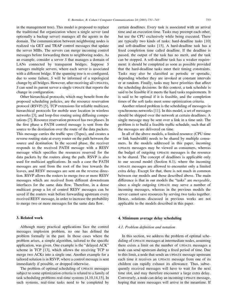
As an example, consider Fig. 1 that shows a three-level

ATM PNNI network. The upper level has a single logical

node, PG(1). This node consists of three logical level-1

nodes: PG(1.1), PG(1.2) and PG(1.3). PG(1.1) consists of

four level-0 (physical) nodes: 1.1.1, 1.1.2, 1.1.3 and 1.1.4.

Similarly, PG(1.2) consists of three-level-0 nodes and

PG(1.3) consists of four level-0 nodes. Suppose that a VC

is set up on link 1.1.3±1.2.2. This VC reduces the available

resources associated with this link. Hence, node 1.1.3 needs

to broadcast an update message to all nodes in PG(1.1).

However, this change affects also the resources and QoS

parameters associated with logical link 1.1±1.2, because

this link summarizes the properties of all physical links

between PG(1.1) and PG(1.2). Hence, node 1.1.4 Ð the

PGL of 1.1 Ð needs to send an update message to the

PGLs of 1.3 and 1.2. Instead of sending such an updateimmediately, which may impose heavy processing burden

on the PGLs, node 1.1.4 may delay the update until receiv-

ing more update messages, either from 1.1.3 regarding link

1.1.3±1.2.2 or from 1.1.2 regarding link 1.1.2±1.2.1. By

merging several update messages, node 1.1.4 as well as

the PGLs of PG(1.2) and PG(1.3), may signi®cantly reduce

the control traf®c exchanged in PG(1) and the processing

load they impose on each other.

As a second example for hierarchical network protocols,

consider distributed network management systems [8,12].

In such systems, multiple management servers are orga-

nized hierarchically. Every server maintains a Management

Information Base (MIB), to allow distributed network

monitoring and control. Each server manages a portion

of the network agents and, in addition to that, plays the

role of an agent to exchange information and accept

control from a higher-level management server (its parent

E. Bortnikov, R. Cohen / Computer Communications 24 (2001) 731±743732

Fig. 1. An ATM PNNI network.

in the management tree). This model is proposed to replace

the traditional ¯at organization where a single server (and

optionally a backup server) manages all the agents in the

domain. The communication between neighboring nodes is

realized via GET and TRAP control messages that update

the server MIBs. The servers can merge incoming control

messages before forwarding them to neighboring nodes. As

an example, consider a server S that manages a domain of

LANs connected by transparent bridges. Suppose S

manages multiple servers, where each server is associated

with a different bridge. If the spanning tree is re-con®gured,

due to some failure, S will be informed of a topological

change by all bridges. However, after receiving all updates,

S can send its parent server a single update that reports the

change in con®guration.

Other hierarchical protocols, which may bene®t from the

proposed scheduling policies, are the resource reservation

protocol (RSVP) [5], TCP extensions for reliable multicast,

hierarchical protocols for mobile user location in wireless

networks [3], and loop-free routing using diffusing compu-

tations [7]. Resource reservation protocol has two phases. In

the ®rst phase a PATH control message is sent from the

source to the destination over the route of the data packets.

This message carries the traf®c spec (Tspec), and creates a

reverse routing state at every router on the path between the

source and destination. In the second phase, the receiver

responds to the received PATH message with a RESV

message which speci®es the resources reserved for the

data packets by the routers along the path. RSVP is also

used for multicast applications. In such a case the PATH

messages are sent from the root of the tree towards the

leaves, and RESV messages are sent on the reverse direc-

tion. RSVP allows the routers to merge two or more RESV

messages which are received from different downstream

interfaces for the same data ¯ow. Therefore, in a dense

multicast group a lot of control RESV messages can be

saved if the routers wait before forwarding upstream every

received RESV message, in order to increase the probability

to merge two or more messages for the same data ¯ow.

3. Related work

Although many practical applications face the control

messages implosion problem, no one has de®ned the

problem formally in the past. In those cases where the

problem arises, a simple algorithm, tailored to the speci®c

application, was given. One example is the ªdelayed ACKº

scheme in TCP [13], which allows the receiving TCP to

merge two ACKs into a single one. Another example for a

tailored solution is in RSVP, where a control message is sent

immediately if possible, or dropped otherwise.

The problem of optimal scheduling of update messages

subject to some optimization criteria is related to a family of

task scheduling problems real-time systems [4,10,14,15]. In

such systems, real-time tasks need to be completed by

certain deadlines. Every task is associated with an arrival

time and an execution time. Tasks may preempt each other,

but use the CPU exclusively while being executed. There

are typically two kinds of tasks: hard-deadline tasks [10]

and soft-deadline tasks [15]. A hard-deadline task has a

®xed completion time called deadline. If the deadline is

passed, the output of the task has no merit, and the task

can be stopped. A soft-deadline task has a weaker require-

ment: it should be completed as soon as possible provided

that the hard-deadline tasks meet their timing constraints.

Tasks may also be classi®ed as periodic or sporadic,

depending whether they are invoked at constant intervals

or at random. Finally, tasks may have priorities that affect

the scheduling decisions. In this context, a task schedule is

said to be feasible if it meets the hard tasks requirements. It

is said to be optimal if it is feasible, and the completion

times of the soft tasks meet some optimization criteria.

Another related problem is the scheduling of messages in

synchronous networks [11]. In this model, a set of messages

should be shipped over the network at certain deadlines. A

single message may be sent over a link in a time unit. The

problem is to build a feasible traf®c schedule, such that all

the messages are delivered on time.

In all of the above models, a limited resource (CPU time

or link bandwidth) needs to be shared by multiple consu-

mers. In the models addressed in this paper, incoming

update messages may be viewed as consumers, whereas

the budget of outgoing update messages is the resource

to be shared. The concept of deadlines is applicable only

to our second model (Section 6.1), where the incoming

update messages are allowed to encounter only a limited

extra delay. Except for that, there is not much in common

between our models and those described above. The main

difference is that in our models the ªtasksº are mergeable,

since a single outgoing update may serve a number of

incoming messages, whereas in the previous models the

server cannot save resources by serving two tasks together.

Hence, solutions discussed in previous works are not

applicable to the models described in this paper.

4. Minimum average delay scheduling

4.1. Problem de®nition and notation

In this section, we address the problem of optimal sche-

duling of update messages at intermediate nodes, assuming

there exists a limit on the number of update messages a

node can send upstream during a ®xed period of time. Due

to this limit, a node that sends an update message upstream

each time it receives an update message from one of its

children can rapidly exhaust its allowance. Thus, subse-

quently received messages will have to wait for the next

time slot, and may therefore encounter a large extra delay.

Conversely, a node can delay an incoming update message,

hoping that more messages will arrive in the meantime. If

E. Bortnikov, R. Cohen / Computer Communications 24 (2001) 731±743 733

more messages indeed arrive, they are all merged into a

single upstream update message. If, however, no additional

update is received, the node will have to send an updateupstream for the received message, and the extra delay turns

to be a ªmistakeº.

The problem is to design a scheduling algorithm that will

run at each node, and determine when a new updatemessage should be sent upstream, while minimizing the

average delay of each received update message. In what

follows, we de®ne the problem formally.

Consider a division of the time domain into time slots of

length t . Suppose that each node must send an updatemessage upstream at the end of every slot. Such a message

is referred to as a mandatory outgoing message. In addition,

every node is allowed to send upstream at most M updatemessages during every slot, namely, between every two

consecutive mandatory messages. These messages are

referred to as optional outgoing messages.

Let Sin � {I1; I2;¼; Ik}; where 0 , I1 , I2 , ¼ , Ik;

denote the arrival times of k incoming update messages

during a time slot. Let Sout � {O1;O2;¼;Ol}; where 0 #O1 , O2 , ¼ , Ol , t and l # M; denote the transmis-

sion times of l outgoing update messages during a time

slot. Sin and Sout will be referred to as the input schedule

and the output schedule, respectively.

We de®ne the extra delay of an incoming updatemessage as the time interval between the arrival of the

message and the transmission of the next outgoing message.

We denote by D i the extra delay of the ith update message,

and de®ne the average extra delay for the whole slot as

1

k

Xk

i�1

Di:

The problem we address is ®nding an optimal schedule for

an (Sin, M) pair. The schedule Sout � {O1;O2;¼;Ol}; where

l # M; is said to be optimal if the following holds:

² There is no other schedule S 0out � {O 01;O02;¼;O 0l 0};

where l 0 # M; that yields a smaller average extra delay

than Sout.

² There is no other schedule S 0out � {O 01;O02;¼;O 0l 0};

where l 0 , l; that yields the same average extra delay

as Sout. This condition guarantees that the optimal solu-

tion does not use unnecessary outgoing messages.

The optimal solution for the period �0; it�; for every i $ 1; is

the union of the optimal solutions for slots

�0; t�; �t; 2t�;¼; ��i 2 1�t; it�: This is because during every

time slot a node can send at most M optional messages

regardless of the number of messages sent during previous

slots, implying that the solutions for every two slots are

independent of each other. Therefore, in order to ®nd an

optimal long-run schedule, it is suf®cient to ®nd the optimal

schedule for each time slot. Without loss of generality, we

shall concentrate upon solving the problem for the ®rst time

slot �0; t� only.

4.2. An optimal off-line algorithm

In the off-line version of the problem, the input schedule

Sin is known in advance, whereas in the on-line version Ii is

known only when the ith message is received. In what

follows, we analyze the optimal solution structure for the

off-line problem and present a naive algorithm that

computes the optimal solution in exponential time. We

then present a dynamic programming algorithm whose

running time complexity is O�Mk2�:Note that a schedule Sout minimizes the average delay if

and only if it minimizes the total extra delayPk

i�1 Di: The

minimum possible total delay for (Sin, M) will be denoted as

D OPT (Sin, M).


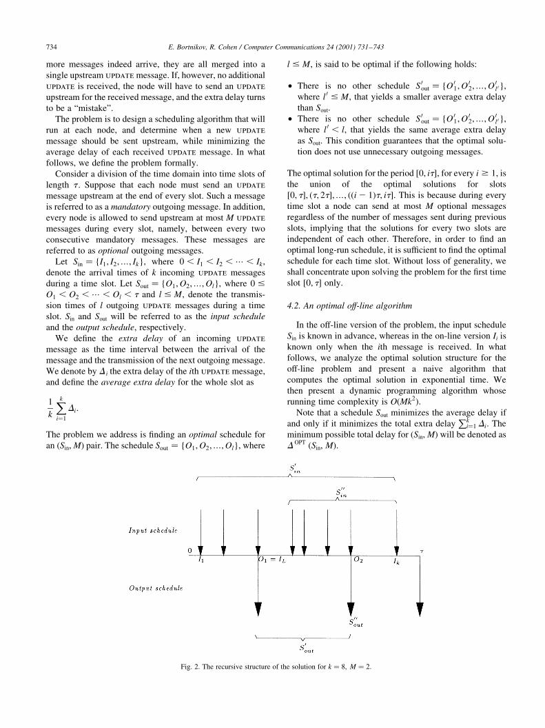
Fig. 2. The recursive structure of the solution for k � 8; M � 2:

In the following, if an update message is sent at time t

following the receipt of an incoming update message, then

the latter is said to be received at t2. The following lemma is

the key observation about the structure of the optimal solution.

Lemma 4.1. Let Sout � {O1;O2;¼;Ol} be an optimal

schedule for (Sin, M). Then, for every j, where 1 # j # l;

there exists an update message whose arrival time is O2j :

Proof. Consider an optimal schedule Sout for which the

lemma does not hold. Hence, there exists a time Oj when

an update message was sent after no message is received.

Observe the last update message that arrived before Oj (if

such a message does not exist, then the messages sent at

O1;¼;Oj are redundant and Sout is not an optimal schedule,

in contradiction to our assumption). Let I2 be the arrival

time of this message. Now, let us change the transmission

time of the j-th message from Oj to I. This results in a new

schedule with the same number of outgoing messages, that

does not increase the extra delay of any message, while

decreasing the delay of at least one message. Hence the

total delay of the new schedule is smaller than the total

delay of Sout, in contradiction to our assumption. B

By Lemma 4.1, each outgoing message in the optimal

solution is sent when some incoming message arrives.

Therefore, the optimal output schedule can be found by an

exhaustive search over allÿ

kM

�possible schedules of M

messages at k times. However, the running time of such

algorithm is exponential. In the following, we present a

dynamic programming algorithm that solves the optimal

off-line scheduling problem in polynomial time. It relies

on the following lemmas:

Lemma 4.2. If M � 0; then

DOPT�Sin;M� � kt 2Xk

i�1

Ii:

Proof. By de®nition, when M � 0; an update message is

sent only at the end of the time slot. Hence, the ith received

update message, that arrives at Ii, encounters a delay of t 2Ii; and

DOPT�Sin; 0� �Xk

i�1

�t 2 Ii� � kt 2Xk

i�1

Ii: A

Lemma 4.3. Let S 0in � {I1; I2;¼; Ik} and M . 0: Let

S 0out � {O1;¼;Ol} be an optimal schedule for �S 0in;M�:Let S 00in � {IiuIi [ S 0in ^ Ii . O1}: Then:

(a) S 0out 2 {O1}is an optimal schedule for �S 00in;M 2 1�:(see Fig. 2).

(b)

DOPT�S 0in;M� �XLi�1

�O1 2 Ii�1 DOPT�S 00in;M 2 1�;

where IL is the arrival time of the last message that

arrived before O1 (see Fig. 2).

Proof.

(a) To prove this part it is suf®cient to show that if S 0out 2{O1} is not an optimal schedule for �S 00in;M 2 1�; then S 0out

is not an optimal schedule for �S 0in;M�: Let S 00out be an

optimal schedule for �S 00in;M 2 1�: An assumption that

S 0out 2 {O1} is not an optimal schedule for �S 00in;M 2 1�implies that it yields a larger total delay for the input

schedule S 00in than S 00out: Hence, the output schedule

{O1} < S 00out yields a smaller total delay for S 0in than

S 0out does, in contradiction to our assumption.

(b) An update message that arrives at Ii # O1 encounters

an extra delay of O1±Ii: Hence, the total extra delay

encountered by all the messages that arrived before O1

isPL

i�1 �O1 2 Ii�: Since by (a) S 0out 2 {O1} is an optimal

schedule for �S 00in;M 2 1�; the total delay encountered by

the remaining update messages is DOPT�S 00in;M 2 1�; and

the claim holds. A

We de®ne the i-suf®x of an input schedule Sin � {I1;¼; Ik}

as the sub-schedule of i last messages in Sin, i.e. Siin �

{Ik2i11;¼; Ik}; where 1 # i # k: We also de®ne S0in as B.

The problem of computing an optimal output schedule for

�Siin;M

0� will be referred to as the �Siin;M

0�-subproblem. By

de®nition, the solution of the original problem is the solu-

tion of the �Skin;M�-subproblem.

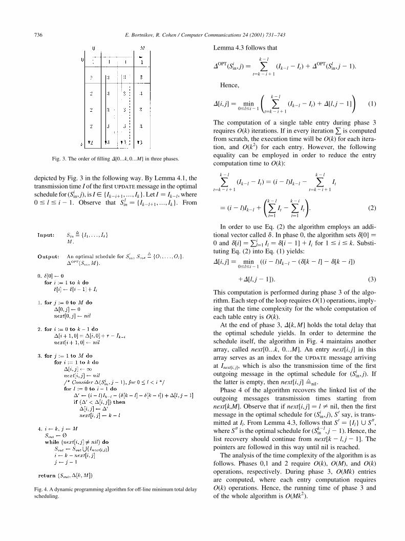
The dynamic programming algorithm operates as

follows. It maintains a two-dimensional array, called

D�0¼k; 0¼M�: At the end of the execution, D�i; j� holds

the total delay of the optimal schedule for �Siin; j�; and there-

fore D�k;M� holds the total delay yielded by the optimal

schedule for the original problem.

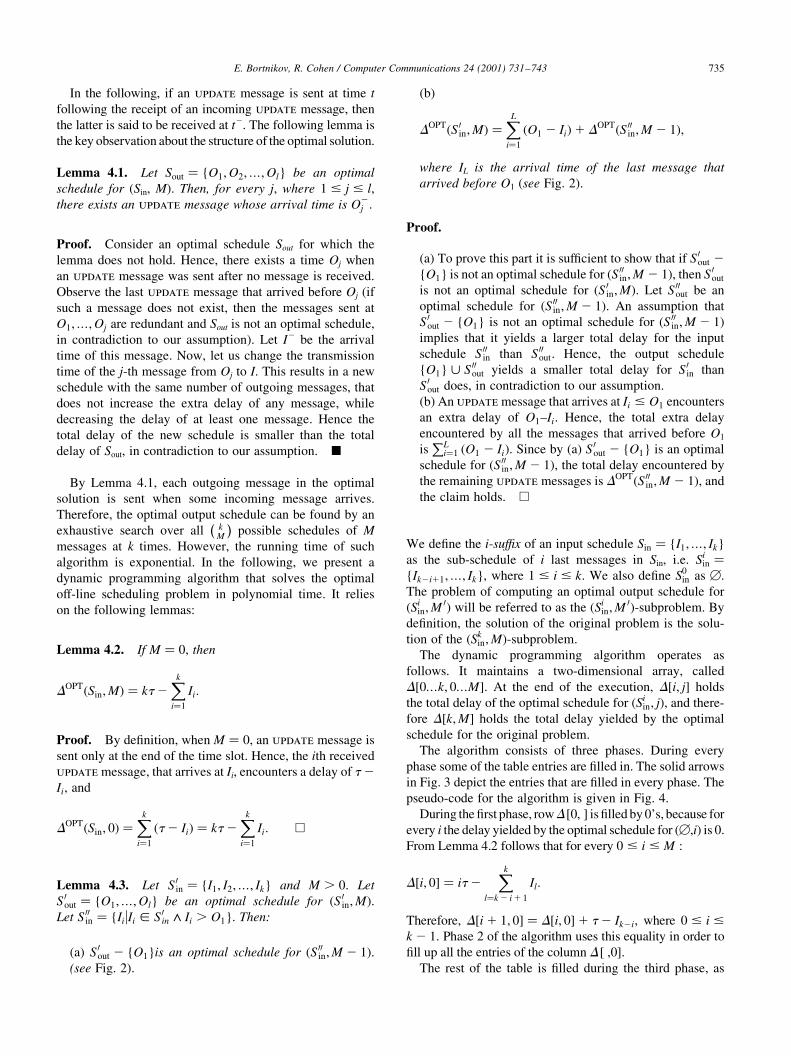
The algorithm consists of three phases. During every

phase some of the table entries are ®lled in. The solid arrows

in Fig. 3 depict the entries that are ®lled in every phase. The

pseudo-code for the algorithm is given in Fig. 4.

During the ®rst phase, rowD[0, ] is ®lled by 0's, because for

every i the delay yielded by the optimal schedule for (B,i) is 0.

From Lemma 4.2 follows that for every 0 # i # M :

D�i; 0� � it 2Xk

l�k 2 i 1 1

Il:

Therefore, D�i 1 1; 0� � D�i; 0�1 t 2 Ik2i; where 0 # i #k 2 1: Phase 2 of the algorithm uses this equality in order to

®ll up all the entries of the column D[ ,0].

The rest of the table is ®lled during the third phase, as


depicted by Fig. 3 in the following way. By Lemma 4.1, the

transmission time I of the ®rst update message in the optimal

schedule for �Siin; j�; is I [ {Ik2i11;¼; Ik}:Let I � Ik2l;where

0 # l # i 2 1: Observe that S lin � {Ik2l11;¼; Ik}: From

Lemma 4.3 follows that

DOPT�Siin; j� �

Xk 2 l

t�k 2 i 1 1

�Ik2l 2 It�1 DOPT�Slin; j 2 1�:

Hence,

D�i; j� � min0#l#i 2 1

Xk 2 l

t�k 2 i 1 1

�Ik2l 2 It�1 D�l; j 2 1� !

�1�

The computation of a single table entry during phase 3

requires O(k) iterations. If in every iterationP

is computed

from scratch, the execution time will be O(k) for each itera-

tion, and O(k2) for each entry. However, the following

equality can be employed in order to reduce the entry

computation time to O(k):

Xk 2 l

t�k 2 i 1 1

�Ik2l 2 It� � �i 2 l�Ik2l 2Xk 2 l

t�k 2 i 1 1

It

� �i 2 l�Ik2l 1Xk 2 l

t�1

It 2Xk 2 i

t�1

It

!: �2�

In order to use Eq. (2) the algorithm employs an addi-

tional vector called d . In phase 0, the algorithm sets d�0� �0 and d�i� � Pi

l�1 Il � d�i 2 1�1 Ii for 1 # i # k: Substi-

tuting Eq. (2) into Eq. (1) yields:

D�i; j� � min0#l#i 2 1

��i 2 l�Ik2l 2 �d�k 2 l�2 d�k 2 i��

1D�l; j 2 1��: (3)

This computation is performed during phase 3 of the algo-

rithm. Each step of the loop requires O(1) operations, imply-

ing that the time complexity for the whole computation of

each table entry is O(k).

At the end of phase 3, D�k;M� holds the total delay that

the optimal schedule yields. In order to determine the

schedule itself, the algorithm in Fig. 4 maintains another

array, called next�0¼k; 0¼M�: An entry next�i; j� in this

array serves as an index for the update message arriving

at Inext[i, j], which is also the transmission time of the ®rst

outgoing message in the optimal schedule for �Siin; j�: If

the latter is empty, then next�i; j� Wnil.

Phase 4 of the algorithm recovers the linked list of the

outgoing messages transmission times starting from

next[k,M]. Observe that if next�i; j� � l ± nil; then the ®rst

message in the optimal schedule for �Siin; j�; S 0 say, is trans-

mitted at Il. From Lemma 4.3, follows that S 0 � {Il} < S 00;where S 00 is the optimal schedule for �Sk2l

in ; j 2 1�: Hence, the

list recovery should continue from next�k 2 l; j 2 1�: The

pointers are followed in this way until nil is reached.

The analysis of the time complexity of the algorithm is as

follows. Phases 0,1 and 2 require O(k), O(M), and O(k)

operations, respectively. During phase 3, O�Mk� entries

are computed, where each entry computation requires

O(k) operations. Hence, the running time of phase 3 and

of the whole algorithm is O�Mk2�:


Fig. 3. The order of ®lling D�0¼k; 0¼M� in three phases.

Fig. 4. A dynamic programming algorithm for off-line minimum total delay

scheduling.

4.3. An alternative de®nition for ªextra delayº

The extra delay de®nition implicitly assumes that the

update messages are independent of each other, because

it aggregates the extra delays regardless of which state vari-

ables each update affects. In practice, this is not always the

case. In the following discussion, two update messages that

affect the same state variable are said to have the same type.

Suppose that two succeeding updates of the same type are

received by a node, and suppose that no outgoing message is

sent between their arrivals. Then, the effect of the ®rst

update terminates upon the arrival of the second one.

Hence, the extra delay the ®rst update encounters is

actually the time interval between the two arrivals.

A small modi®cation in the dynamic programming algo-

rithm can be made in order to compute an optimal schedule

under the new de®nition. First, note that Lemma 4.1 still holds.

Now, let O and O 0, where O , O 0;be the transmission times of

two consecutive outgoing messages. Let the arrival times of all

the updates of the same type received between O and O 0 be

I 01 , ¼ , I 0l: By the new de®nition, these messages encoun-

ter extra delays of I 02 2 I 01; I03 2 I 02;¼; I 0l 2 I 0l21; and O 0 2 I 0l;

respectively. Hence, the total extra delay encountered by all

these messages is O 0 2 I 01: This is exactly the extra delay

encountered by the ®rst update according to the original

de®nition. Therefore, in order to use the existing algorithm

for computing an optimal schedule under the new de®nition,

one has to limit the summation of extra delays only to the ®rst

message of every type the node receives after the last updatetransmission.

5. On-line algorithms for minimum average delayscheduling

In this section, we present a family of simple on-line

heuristics for the minimum average delay-scheduling

problem. These heuristics try to imitate the following beha-

vior of the optimal algorithm. On one hand, the optimal

algorithm ªrecognizesº bursts of incoming messages in

the input schedule, and reacts on each burst by sending an

update message. On the other hand, the optimal algorithm

balances the delays that incoming messages encounter, by

not delaying a large group of messages for a long period of

time while serving another group of comparable size

quickly.

The simplest heuristic is referred to as Greedy. As long as

it has used less than M outgoing messages, Greedy sends an

outgoing message in response to each incoming message. If

the allowance is exhausted, it delays each arriving message

until the end of the slot. Hence, Greedy performs optimally

on input schedules of size M or less, but may yield an

average delay close to t for heavily loaded inputs.

The second heuristic is referred to as EqualPart. The

scheduler divides the interval �0; t� to M 1 1 equal sub-

slots, and outgoing messages are sent only at the end of

each sub-slot. If no incoming message arrives during

some sub-slot, an outgoing message is not sent at the end

of the sub-slot.

The EqualPart algorithm provides the following guaran-

tees regardless of the input schedule size. First, the maxi-

mum delay a message encounters is �t=�M 1 1��: Second, if

the incoming messages are generated by a Poisson process,

the expected average delay is �t=2�M 1 1��: The main disad-

vantage of this algorithm is its performance under a lightly

loaded arrival schedule, where Greedy serves incoming

messages very fast.

In the following, we use simulations in order to compare

the performance of the heuristics to the performance of the

optimal algorithm. The slot size is t � 100; the average size

of the schedules varies from 5 to 200, and the maximum

number of outgoing messages is 10. For every average size


Fig. 5. The performance of Greedy and Equalpart.

of the input schedule, each algorithm was executed on 500

different exponentially distributed input schedules, and the

received results were averaged.

Fig. 5 depicts the performance of Greedy and EqualPart

versus the optimal (off-line) algorithm. As expected, Greedy

performs well for lightly loaded schedules, but becomes

impractical as the input load increases (see Fig. 5(a)). In

contrast, the performance of EqualPart improves as the

input schedule becomes heavier loaded (Fig. 5(b)).

EqualPart does not use outgoing messages that are sched-

uled to be sent at the end of empty sub-slots. Hence, it may

send less than M outgoing messages even when the number

of incoming messages is larger than M. In what follows,

we propose two variations of EqualPart that avoid this

weakness.

The ®rst variation, referred to as TokenAlgorithm, uses

the notion of tokens. At the beginning of a slot, the algo-

rithm has 0 tokens. When an update message arrives, the

algorithm operates as follows:

² If the number of tokens is greater than 0, an outgoing

message is immediately sent and the number of tokens

decreases by 1.

² Otherwise, the message is delayed until the end of the

sub-slot.

At the end of the sub-slot, the algorithm operates as

follows:

² If there is no waiting message, the token pool grows by 1.

² Otherwise, an outgoing message is sent immediately, and

the number of tokens does not change.

BalanceAlgorithm is another variation of EqualPart. Like

TokenAlgorithm, it uses the notion of tokens, but uses them

in a less greedy way, because each saved token reduces the

length of all remaining sub-slots. Let n denote the number of

update messages a node can send until the end of the slot,

and T denote the time remaining until the end of the slot.

When the slot starts, n is initialized to M 1 1 and T to t . The

length of each sub-slot is determined at the end of the

previous sub-slot as T =n: Hence, the ®rst sub-slot ends at

�t=�M 1 1��. If during a sub-slot i there is no incoming

message, no update message is sent at the end of the sub-

slot, and �T Ã T 2 �T =n�� whereas n does not change.

Consequently, each of the remaining sub-slots is shorter

than sub-slot i. If an incoming message does arrive during

sub-slot i, an update is sent at the end of the sub-slot, �T ÃT 2 �T=n�� and n Ã n 2 1: Consequently, the length of sub-

slot i 1 1 is equal to the length of sub-slot i.

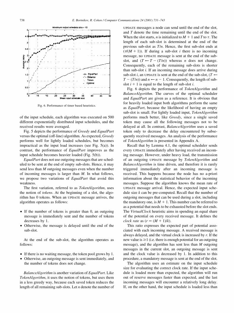
Fig. 6 depicts the performance of TokenAlgorithm and

BalanceAlgorithm. The curves of the optimal scheduler

and EqualPart are given as a reference. It is obvious that

for heavily loaded input both algorithms perform the same

as EqualPart, because the likelihood of having an empty

sub-slot is small. For lightly loaded input, TokenAlgorithm

performs much better, like Greedy, since a single saved

token may cause all the following messages not to be

delayed at all. In contrast, BalanceAlgorithm uses a saved

token only to decrease the delay encountered by subse-

quently received messages. An analysis of the performance

of TokenAlgorithm is presented in Appendix A.

Recall that by Lemma 4.1, the optimal scheduler sends

every update immediately after having received an incom-

ing message. However, under heavy load, the transmission

of an outgoing update message by TokenAlgorithm and

BalanceAlgorithm is time driven, and therefore it is rarely

triggered immediately after an incoming message is

received. This happens because the node has no a-priori

information about the statistical behavior of the incoming

messages. Suppose the algorithm knows the mean rate of

update message arrival. Hence, the expected input sche-

dule size k can be pre-computed. Recall that the number of

outgoing messages that can be used during a slot, including

the mandatory one, is M 1 1: This number can be referred to

as a potential that needs to be exhausted before the slot ends.

The VirtualClock heuristic aims in spending an equal share

of the potential on every received message. It de®nes the

clock rate as �r � �M 1 1�=k�:This ratio expresses the expected part of potential asso-

ciated with each incoming message. A received message is

always delayed, and the virtual clock is increased by r. If the

new value is $1 (i.e. there is enough potential for an outgoing

message), and the algorithm has sent less than M outgoing

messages in the current slot, an outgoing message is sent

and the clock value is decreased by 1. In addition to this

procedure, a mandatory message is sent at the end of the slot.

The algorithm uses an estimate on the input schedule

size for evaluating the correct clock rate. If the input sche-

dule is loaded more than expected, the algorithm will run

out of reserve messages faster than expected, and the last

incoming messages will encounter a relatively long delay.

If, on the other hand, the input schedule is loaded less than


Fig. 6. Performance of timer based heuristics.

expected, the algorithm may use less than M optional

messages.

VirtualClock overcomes an inherent problem of all the

timer-based approaches, namely their inability to recognize

bursts in the input schedule and to react accordingly. When

a burst of incoming messages is received, VirtualClock may

trigger the transmission of an outgoing update message

even if the previous message has just been sent. On the

other hand, it may delay for a long time an isolated incom-

ing message that does not affect the average delay signi®-

cantly. The ideas behind this heuristic are similar to those

behind Lixia Zhang's traf®c control algorithm for packet

switching networks, which is also called VirtualClock

[6,16].

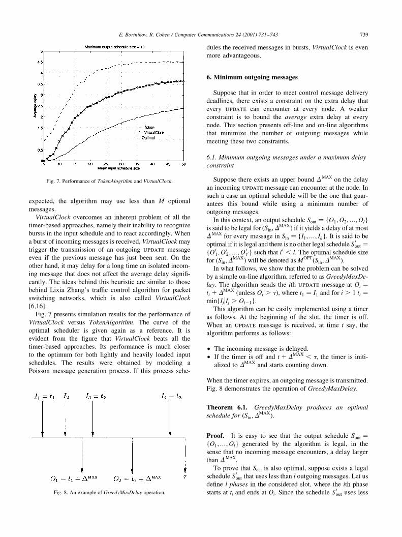
Fig. 7 presents simulation results for the performance of

VirtualClock versus TokenAlgorithm. The curve of the

optimal scheduler is given again as a reference. It is

evident from the ®gure that VirtualClock beats all the

timer-based approaches. Its performance is much closer

to the optimum for both lightly and heavily loaded input

schedules. The results were obtained by modeling a

Poisson message generation process. If this process sche-

dules the received messages in bursts, VirtualClock is even

more advantageous.

6. Minimum outgoing messages

Suppose that in order to meet control message delivery

deadlines, there exists a constraint on the extra delay that

every update can encounter at every node. A weaker

constraint is to bound the average extra delay at every

node. This section presents off-line and on-line algorithms

that minimize the number of outgoing messages while

meeting these two constraints.

6.1. Minimum outgoing messages under a maximum delay

constraint

Suppose there exists an upper bound DMAX on the delay

an incoming update message can encounter at the node. In

such a case an optimal schedule will be the one that guar-

antees this bound while using a minimum number of

outgoing messages.

In this context, an output schedule Sout � {O1;O2;¼;Ol}

is said to be legal for �Sin;DMAX� if it yields a delay of at most

DMAX for every message in Sin � {I1;¼; Ik}: It is said to be

optimal if it is legal and there is no other legal schedule S 0out �{O 01;O

02;¼;O 0l 0} such that l 0 , l: The optimal schedule size

for �Sin;DMAX� will be denoted as MOPT�Sin;D

MAX�:In what follows, we show that the problem can be solved

by a simple on-line algorithm, referred to as GreedyMaxDe-

lay. The algorithm sends the ith update message at Oi �ti 1 DMAX (unless Oi . t), where t1 � I1 and for i . 1 ti �min{IjuIj . Oi21}:

This algorithm can be easily implemented using a timer

as follows. At the beginning of the slot, the timer is off.

When an update message is received, at time t say, the

algorithm performs as follows:

² The incoming message is delayed.

² If the timer is off and t 1 DMAX , t; the timer is initi-

alized to DMAX and starts counting down.

When the timer expires, an outgoing message is transmitted.

Fig. 8 demonstrates the operation of GreedyMaxDelay.

Theorem 6.1. GreedyMaxDelay produces an optimal

schedule for �Sin;DMAX�:

Proof. It is easy to see that the output schedule Sout �{O1;¼;Ol} generated by the algorithm is legal, in the

sense that no incoming message encounters, a delay larger

than DMAX.

To prove that Sout is also optimal, suppose exists a legal

schedule S 0out that uses less than l outgoing messages. Let us

de®ne l phases in the considered slot, where the ith phase

starts at ti and ends at Oi. Since the schedule S 0out uses less


Fig. 7. Performance of TokenAlogrithm and VirtualClock.

Fig. 8. An example of GreedyMaxDelay operation.

than l messages, there is necessarily a phase, say i, where

S 0out sends no message. This implies that the incoming

message that arrives at ti encounters a delay of more

than DMAX. Hence, S 0out is illegal, in contradiction to our

assumption. A

6.2. Minimum outgoing messages under an average delay

constraint

The last problem we address is ®nding an optimal sche-

dule while bounding the average delay. In this context, an

output schedule Sout � {O1;O2;¼;Ol} is said to be legal for

�Sin;DAVG� if it yields an average delay of at most D AVG for

Sin � {I1;¼; Ik}: It is said to be optimal if it is legal and

there is no other legal schedule S 0out � {O 01;O02;¼;O 0l 0}

such that l 0 , l: The optimal schedule size for �Sin;DAVG�

will be denoted as MOPT�Sin;DAVG�:

An off-line solution for the problem can be found using a

variation of the algorithm for minimum average delay sche-

duling (Section 4). By de®nition, for every M $ 0 and Sin

DOPT�Sin;M� $ DOPT�Sin;M11�:Hence, if �DOPT�Sin;M��=k . DAVG holds for some M, no

output schedule of size M or less can yield an average

delay of D AVG or less for Sin. Therefore, MOPT(Sin,DAVG) is

the smallest value of M that ful®lls:

DOPT�Sin;M�k

# DAVG:

Once MOPT is determined, a possible optimal schedule is the

one that yields the minimum average delay for (Sin, MOPT).

MOPT�Sin;DAVG� can be found by performing a binary

search on the interval �1;¼; k�; invoking the dynamic

programming algorithm described in Section 4 at each

step. Such a search would require log2 k steps. However, a

single invocation of the dynamic programming algorithm

would suf®ce if the following modi®cation is made. The

modi®ed algorithm maintains a table D�0¼k; � of k 1 1

rows and a dynamic number of columns. Columns are

added to D and computed one by one, until j for

which �D�k; j�=k� # DAVG is found. The time complexity

of the algorithm is O�MOPT�Sin;DAVG�k2�: Since

MOPT�Sin;DAVG� # k;O�k3� is an upper bound.

In what follows we discuss two possible on-line heuristics

for the problem. The GreedyMaxDelay algorithm presented

in Section 6.1 is one possible solution. It produces a legal

output schedule by guaranteeing a delay of at most D AVG for

each incoming message. However, the produced schedule is

likely to be inef®cient because an optimal schedule may

delay some messages longer than D AVG.

A better heuristic is the GreedyAverageDelay algorithm.

This algorithm delays the next outgoing message as long as

the average delay of all the messages received after the

transmission of the last outgoing update does not exceed

D AVG. Let Bi � {IjuOi21 , Ij # Oi}; where O0 W 0: Then,

the algorithm ful®lls the following for every 1 # i # l:XI[Bi

�Oi 2 I�

uBiu� DAVG

: �4�

The only difference between this algorithm and the Greedy-

MaxDelay is that if an update message arrives at time t and

the timer is on, scheduled to expire at t 0, its expiration is

rescheduled to t 0 1 �DAVG 2 �t 0 2 t��=l; where l is the

number of waiting messages at t1 (i.e. including the new

one). If t 0 $ t; the timer is turned off. It is easy to verify that

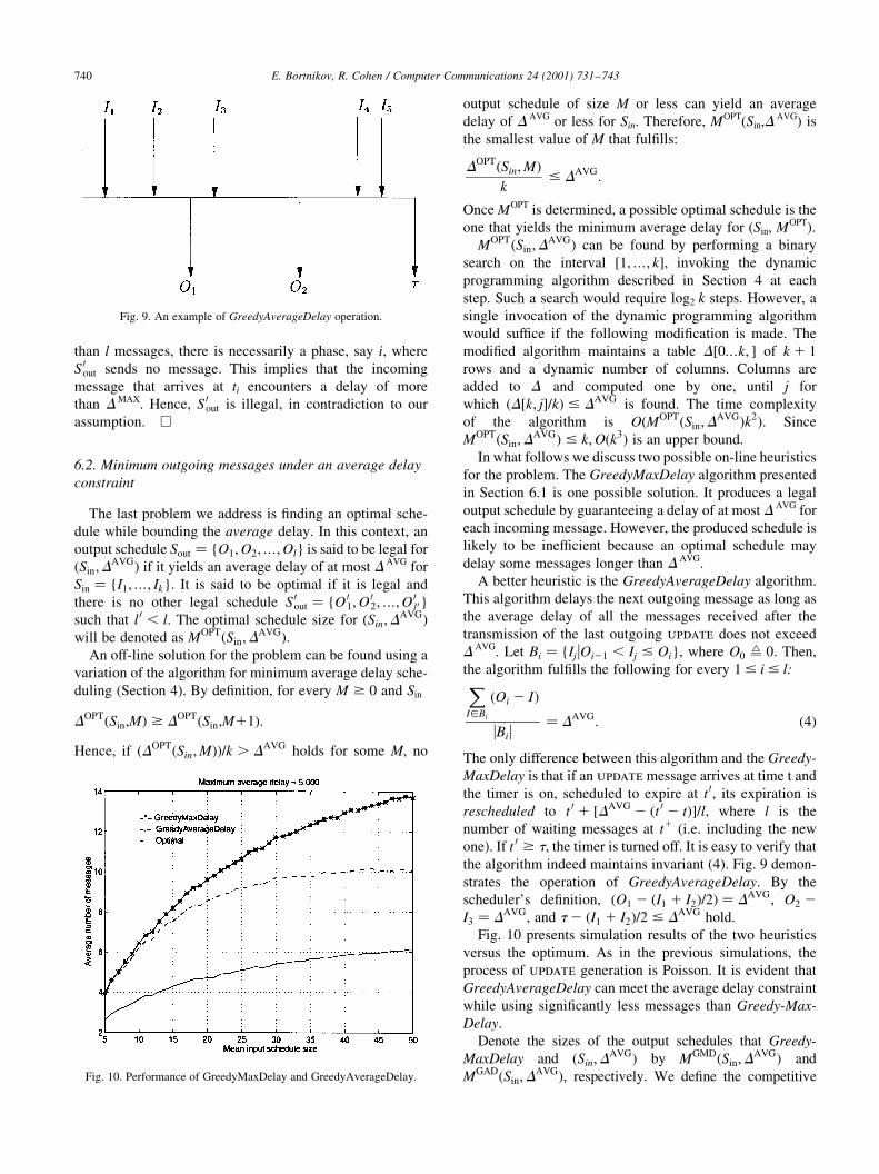
the algorithm indeed maintains invariant (4). Fig. 9 demon-

strates the operation of GreedyAverageDelay. By the

scheduler's de®nition, �O1 2 �I1 1 I2�=2� � DAVG; O2 2

I3 � DAVG; and t 2 �I1 1 I2�=2 # DAVG hold.

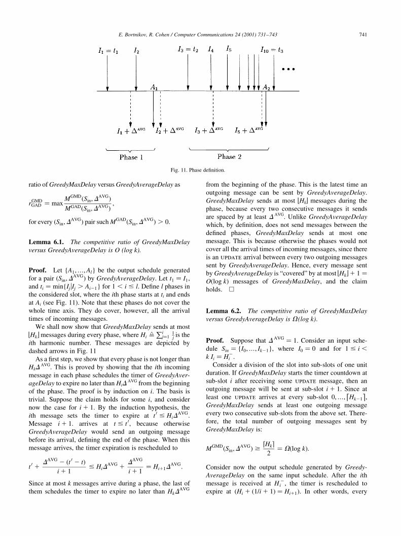
Fig. 10 presents simulation results of the two heuristics

versus the optimum. As in the previous simulations, the

process of update generation is Poisson. It is evident that

GreedyAverageDelay can meet the average delay constraint

while using signi®cantly less messages than Greedy-Max-

Delay.

Denote the sizes of the output schedules that Greedy-

MaxDelay and �Sin;DAVG� by MGMD�Sin;D

AVG� and

MGAD�Sin;DAVG�; respectively. We de®ne the competitive


Fig. 9. An example of GreedyAverageDelay operation.

Fig. 10. Performance of GreedyMaxDelay and GreedyAverageDelay.

ratio of GreedyMaxDelay versus GreedyAverageDelay as

rGMDGAD � max

MGMD�Sin;DAVG�

MGAD�Sin;DAVG� ;

for every �Sin;DAVG� pair such MGAD�Sin;D

AVG� . 0:

Lemma 6.1. The competitive ratio of GreedyMaxDelay

versus GreedyAverageDelay is O (log k).

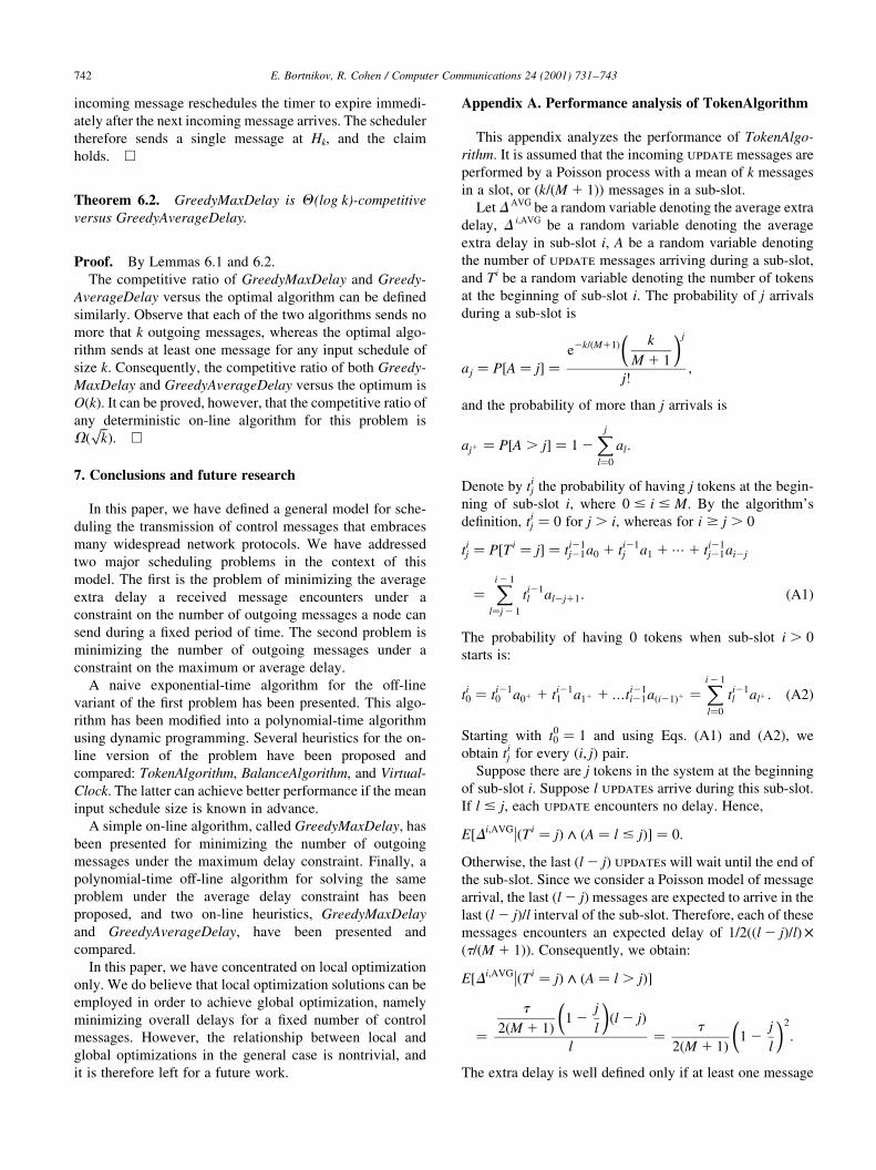
Proof. Let {A1;¼;Al} be the output schedule generated

for a pair �Sin;DAVG� by GreedyAverageDelay. Let t1 � I1;

and ti � min{IjuIj . Ai21} for 1 , i # l: De®ne l phases in

the considered slot, where the ith phase starts at ti and ends

at Ai (see Fig. 11). Note that these phases do not cover the

whole time axis. They do cover, however, all the arrival

times of incoming messages.

We shall now show that GreedyMaxDelay sends at most

bHkc messages during every phase, where Hi WPi

j�11jis the

ith harmonic number. These messages are depicted by

dashed arrows in Fig. 11

As a ®rst step, we show that every phase is not longer than

HkDAVG. This is proved by showing that the ith incoming

message in each phase schedules the timer of GreedyAver-

ageDelay to expire no later than HiDAVG from the beginning

of the phase. The proof is by induction on i. The basis is

trivial. Suppose the claim holds for some i, and consider

now the case for i 1 1: By the induction hypothesis, the

ith message sets the timer to expire at t 0 # HiDAVG

:

Message i 1 1: arrives at t # t 0; because otherwise

GreedyAverageDelay would send an outgoing message

before its arrival, de®ning the end of the phase. When this

message arrives, the timer expiration is rescheduled to

t 0 1DAVG 2 �t 0 2 t�

i 1 1# HiD

AVG 1DAVG

i 1 1� Hi11D

AVG:

Since at most k messages arrive during a phase, the last of

them schedules the timer to expire no later than HkDAVG

from the beginning of the phase. This is the latest time an

outgoing message can be sent by GreedyAverageDelay.

GreedyMaxDelay sends at most bHkc messages during the

phase, because every two consecutive messages it sends

are spaced by at least D AVG. Unlike GreedyAverageDelay

which, by de®nition, does not send messages between the

de®ned phases, GreedyMaxDelay sends at most one

message. This is because otherwise the phases would not

cover all the arrival times of incoming messages, since there

is an update arrival between every two outgoing messages

sent by GreedyAverageDelay. Hence, every message sent

by GreedyAverageDelay is ªcoveredº by at most bHkc 1 1 �O�log k� messages of GreedyMaxDelay, and the claim

holds. A

Lemma 6.2. The competitive ratio of GreedyMaxDelay

versus GreedyAverageDelay is V (log k).

Proof. Suppose that DAVG � 1: Consider an input sche-

dule Sin � {I0;¼; Ik21}; where I0 � 0 and for 1 # i ,k Ii � H2

i :

Consider a division of the slot into sub-slots of one unit

duration. If GreedyMaxDelay starts the timer countdown at

sub-slot i after receiving some update message, then an

outgoing message will be sent at sub-slot i 1 1: Since at

least one update arrives at every sub-slot 0;¼;�Hk21

�;

GreedyMaxDelay sends at least one outgoing message

every two consecutive sub-slots from the above set. There-

fore, the total number of outgoing messages sent by

GreedyMaxDelay is:

MGMD�Sin;DAVG� $

Hkd e2� V�log k�:

Consider now the output schedule generated by Greedy-

AverageDelay on the same input schedule. After the ith

message is received at H 2i ; the timer is rescheduled to

expire at �Hi 1 �1=i 1 1� � Hi11�: In other words, every


Fig. 11. Phase de®nition.

incoming message reschedules the timer to expire immedi-

ately after the next incoming message arrives. The scheduler

therefore sends a single message at Hk, and the claim

holds. A

Theorem 6.2. GreedyMaxDelay is Q (log k)-competitive

versus GreedyAverageDelay.

Proof. By Lemmas 6.1 and 6.2.

The competitive ratio of GreedyMaxDelay and Greedy-

AverageDelay versus the optimal algorithm can be de®ned

similarly. Observe that each of the two algorithms sends no

more that k outgoing messages, whereas the optimal algo-

rithm sends at least one message for any input schedule of

size k. Consequently, the competitive ratio of both Greedy-

MaxDelay and GreedyAverageDelay versus the optimum is

O(k). It can be proved, however, that the competitive ratio of

any deterministic on-line algorithm for this problem is

V� ��kp �: A

7. Conclusions and future research

In this paper, we have de®ned a general model for sche-

duling the transmission of control messages that embraces

many widespread network protocols. We have addressed

two major scheduling problems in the context of this

model. The ®rst is the problem of minimizing the average

extra delay a received message encounters under a

constraint on the number of outgoing messages a node can

send during a ®xed period of time. The second problem is

minimizing the number of outgoing messages under a

constraint on the maximum or average delay.

A naive exponential-time algorithm for the off-line

variant of the ®rst problem has been presented. This algo-

rithm has been modi®ed into a polynomial-time algorithm

using dynamic programming. Several heuristics for the on-

line version of the problem have been proposed and

compared: TokenAlgorithm, BalanceAlgorithm, and Virtual-

Clock. The latter can achieve better performance if the mean

input schedule size is known in advance.

A simple on-line algorithm, called GreedyMaxDelay, has

been presented for minimizing the number of outgoing

messages under the maximum delay constraint. Finally, a

polynomial-time off-line algorithm for solving the same

problem under the average delay constraint has been

proposed, and two on-line heuristics, GreedyMaxDelay

and GreedyAverageDelay, have been presented and

compared.

In this paper, we have concentrated on local optimization

only. We do believe that local optimization solutions can be

employed in order to achieve global optimization, namely

minimizing overall delays for a ®xed number of control

messages. However, the relationship between local and

global optimizations in the general case is nontrivial, and

it is therefore left for a future work.

Appendix A. Performance analysis of TokenAlgorithm

This appendix analyzes the performance of TokenAlgo-

rithm. It is assumed that the incoming update messages are

performed by a Poisson process with a mean of k messages

in a slot, or �k=�M 1 1�� messages in a sub-slot.

Let D AVG be a random variable denoting the average extra

delay, D i,AVG be a random variable denoting the average

extra delay in sub-slot i, A be a random variable denoting

the number of update messages arriving during a sub-slot,

and Ti be a random variable denoting the number of tokens

at the beginning of sub-slot i. The probability of j arrivals

during a sub-slot is

aj � P�A � j� �e2k=�M11� k

M 1 1

� �j

j!;

and the probability of more than j arrivals is

aj1 � P�A . j� � 1 2Xj

l�0

al:

Denote by tij the probability of having j tokens at the begin-

ning of sub-slot i, where 0 # i # M: By the algorithm's

de®nition, tij � 0 for j . i; whereas for i $ j . 0

tij � P�Ti � j� � ti21

j21a0 1 ti21j a1 1 ¼ 1 ti21

j21ai2j

�Xi 2 1

l�j 2 1

ti21l al2j11: �A1�

The probability of having 0 tokens when sub-slot i . 0

starts is:

ti0 � ti21

0 a01 1 ti211 a11 1 ¼ti21

i21a�i21�1 �Xi 2 1

l�0

ti21l al1 : �A2�

Starting with t00 � 1 and using Eqs. (A1) and (A2), we

obtain tij for every (i, j) pair.

Suppose there are j tokens in the system at the beginning

of sub-slot i. Suppose l updates arrive during this sub-slot.

If l # j; each update encounters no delay. Hence,

E�Di;AVGu�Ti � j� ^ �A � l # j�� 0:

Otherwise, the last �l 2 j� updates will wait until the end of

the sub-slot. Since we consider a Poisson model of message

arrival, the last �l 2 j�messages are expected to arrive in the

last �l 2 j�=l interval of the sub-slot. Therefore, each of these

messages encounters an expected delay of 1=2��l 2 j�=l� ��t=�M 1 1��: Consequently, we obtain:

E�Di;AVGu�Ti � j� ^ �A � l . j��

�t

2�M 1 1� 1 2j

l

� ��l 2 j�

l� t

2�M 1 1� 1 2j

l

� �2

:

The extra delay is well de®ned only if at least one message


is received during a sub-slot. The probability of receiving

l . 0 updateS during a sub-slot given that the sub-slot is

non-empty is

p�A � l . 0uA . 0� � al

a01

:

Hence,

E�Di;AVGuTi � j� � t

2�M 1 1�X1

l�j 1 1

1 2j

l

� �2 al

a01

;

and

E�Di;AVG� � t

2�M 1 1�Xi

j�0

tji

X1i�j 1 1

1 2j

l

� �2 al

a01

:

Since the incoming message generation process is Poisson,

an update message has an equal probability to be received

in every sub-slot, namely �1=�M 1 1��: For every 0 # i #M; a message arriving at sub-slot i encounters an expected

extra delay of E[Di,AVG]. Hence

E�DAVG� �

XMi�0

E�Di;AVG�M 1 1

:

These results give the same performance curve shown in

Fig. 6

References

[1] A. Alles, ATM internetworking, Engineering InterOp, Las Vegas,

March 1995.

[2] ATM Forum PNNI SWG 94-0471R13. ATM Forum PNNI Draft

Speci®cations, April 1994.

[3] B. Awerbuch, D. Peleg. Concurrent on-line tracking of mobile users,

SIGOMM, September 1991, pp. 221±233.

[4] S. Baruah, G. Koren, B. Mishra, A. Raghunathan, L. Rosier, D.

Shasha, On-line scheduling in the presence of overload, 32nd Sympo-

sium on Foundations of Computer Science, 1991, pp. 100±110.

[5] R. Braden, L. Zhang. S. Berson, S. Herzog, S. Jamin, Resource reser-

vation protocol (RSVP), RFC-2205, September 1997.

[6] D. Clark, S. Shenker, L. Zhang, Supporting real-time applications in

an integrated service packet network: Architecture and mechanisms,

SIGCOMM, 1992.

[7] J.J. Garcia-Luna-Aceves, Loop-free routing using diffusing computa-

tions, IEEE Transactions on Networking 1 (1) (1993).

[8] G. Goldszmidt, Distributed system management via elastic servers,

IEEE First International Workshop on Systems Management, Los

Angeles, CA, April 1993, pp. 31±35.

[9] C. Huitema, Routing in the Internet, Prentice-Hall, Englewoods

Cliffs, NJ, 1995.

[10] C.L. Liu, J.W. Layland, Scheduling algorithms for multiprogramming

in a hard real time environment, JACM 20 (1) (1973) 46±61.

[11] K.-S. Lui, S. Zaks, Scheduling in synchronous networks and the

greedy algorithm, WDAG, 1997.

[12] K. Meyer, M. Erlinger, J. Betserand, C. Sunshine, G. Goldszmidt, Y.

Yemini, Decentralizing control and intelligence in network manage-

ment, The Fourth International Symposium on Integrated Network

Management, May 1995.

[13] W. Richard Stevens, TCP/IP Illustrated, Addison-Wesley, Reading,

MA, 1994.

[14] J.K. Strosnider, J.P. Lehoczky, L. Sha, The deferrable server algo-

rithm for enhanced aperiodic responsiveness in hard real-time envir-

onments, IEEE Transactions on Computers 44 (1) (1995) 73±89.

[15] T.-S. Tia, J.W.-S. Liu, M. Shankar, Algorithms and optimality of

scheduling soft aperiodic request in ®xed-priority preempted systems,

Journal of Real-Time Systems 10 (1): 23±43, January 1996.

[16] L. Zhang, Virtual clock: A new traf®c control algorithm for packet

switching networks, ACM Transactions on Computer Systems 9 (2)

(1991) 101±124.


Documents

Schemes for scheduling control messages by hierarchical protocols