Embed Size (px)
Citation preview
Schelling’s Bounded Neighbourhood Model: A systematic
investigation
Ali J E H Afshar Dodson
PhD
University of York
Computer Science
April 2014

ii
Abstract
This thesis explores the role of modelling and computational simulation, in relation to social
systems, with specific focus on Schelling’s Bounded Neighbourhood Model. It discusses the
role of computational modelling and some techniques that can be used in the Social sciences.
Simulation of social interaction consistently creates debate in the Social sciences. However,
most models are dismissed as either too simplistic or unrealistic. In an attempt to counter
these criticisms, more complex models have been developed. However, by increasing the com-
plexity of the model, the underlying dynamics can be lost. Schelling’s models of segregation
are a classic example, with much of the work building on his simple segregation model. The
complexity of the models being developed are such that, real world implications are being in-
ferred from the results. The Complex Systems Modelling and Simulation (CoSMoS) process
has a proven track record in developing simulations of complex models. In a novel appli-
cation, the CoSMoS process is applied to Schelling’s Bounded Neighbourhood Model. The
process formalises Schelling’s Bounded Neighbourhood Model and develops a simulation. The
simulation is validated against the results from Schelling’s model and then used to question
the model. The questioning of the model is an attempt to examine the underlying dynamics
of the segregation model. In this respect, two measures, static and dynamic, are used in
the analysis of the results. Initally, the e↵ect of ordered movement was tested by chang-
ing the movement, from ordered to random. A second experiment examined agents’ perfect
knowledge of the system. By introducing a sample, the agents’ knowledge of the system is
reduced. The third experiment introduced a friction parameter, to examine the e↵ect of ease
of movement into and out of the neighbourhood. In the final experiment, Schelling’s model
is recast as a network model. Although the recasting of the model is slightly unorthodox, it
opens the model up to network analysis. This analysis allows the easy definition of a ‘social
network’ that is overlaid on Schelling’s ‘neighbourhood network’. Two di↵erent networks are
applied, Random and Small World. The results of the experiments showed, that Schelling’s
model is remarkably robust. Whilst the adjustments to the model all contributed to changes
in the output, the only significant di↵erence occurred when the social network was added.
iii

iv ABSTRACT
Contents
Abstract iii
List of Figures vii
List of Tables viii
Acknowledgements xv
Authour’s declaration xvii
1 Introduction 1
2 Modelling Social Systems 5
2.1 Di↵erential Equations . . . . . . . . . . . . . . . . . . . . . . . . . . . . . . . 5
2.2 Cellular Automata . . . . . . . . . . . . . . . . . . . . . . . . . . . . . . . . . 8
2.3 Game Theory . . . . . . . . . . . . . . . . . . . . . . . . . . . . . . . . . . . . 12
2.4 Networks . . . . . . . . . . . . . . . . . . . . . . . . . . . . . . . . . . . . . . 14
2.5 Agent Based Modelling . . . . . . . . . . . . . . . . . . . . . . . . . . . . . . 19
2.6 Geographic Information Systems . . . . . . . . . . . . . . . . . . . . . . . . . 23
2.7 Summary . . . . . . . . . . . . . . . . . . . . . . . . . . . . . . . . . . . . . . 26
3 Models of Segregation 29
3.1 Spatial Proximity Model . . . . . . . . . . . . . . . . . . . . . . . . . . . . . . 29
3.2 Bounded Neighbourhood Model . . . . . . . . . . . . . . . . . . . . . . . . . . 37
3.3 Tipping Model . . . . . . . . . . . . . . . . . . . . . . . . . . . . . . . . . . . 42
3.4 A critique of the Bounded Neighbourhood Model . . . . . . . . . . . . . . . . 44
3.5 Conclusions . . . . . . . . . . . . . . . . . . . . . . . . . . . . . . . . . . . . . 45
3.6 Further work on Schelling . . . . . . . . . . . . . . . . . . . . . . . . . . . . . 46
v
vi CONTENTS
4 Methodology 49
4.1 Verification . . . . . . . . . . . . . . . . . . . . . . . . . . . . . . . . . . . . . 49
4.2 Validation . . . . . . . . . . . . . . . . . . . . . . . . . . . . . . . . . . . . . . 51
4.3 The Complex System Modelling and Simulation process . . . . . . . . . . . . 52
4.4 Hypothesis Testing . . . . . . . . . . . . . . . . . . . . . . . . . . . . . . . . . 55
4.5 Experimental structure . . . . . . . . . . . . . . . . . . . . . . . . . . . . . . . 61
5 Formalising the Bounded Neighbourhood Model 63
5.1 Developing the Domain Model . . . . . . . . . . . . . . . . . . . . . . . . . . 63
5.2 Platform Model . . . . . . . . . . . . . . . . . . . . . . . . . . . . . . . . . . . 73
5.3 Simulation Platform . . . . . . . . . . . . . . . . . . . . . . . . . . . . . . . . 76
5.4 Results Model . . . . . . . . . . . . . . . . . . . . . . . . . . . . . . . . . . . . 78
5.5 Summary . . . . . . . . . . . . . . . . . . . . . . . . . . . . . . . . . . . . . . 78
6 Whose move is it anyway? 81
6.1 Introduction . . . . . . . . . . . . . . . . . . . . . . . . . . . . . . . . . . . . . 81
6.2 Hypothesis . . . . . . . . . . . . . . . . . . . . . . . . . . . . . . . . . . . . . 81
6.3 Domain model . . . . . . . . . . . . . . . . . . . . . . . . . . . . . . . . . . . 83
6.4 Platform Model . . . . . . . . . . . . . . . . . . . . . . . . . . . . . . . . . . . 83
6.5 Simulation Platform . . . . . . . . . . . . . . . . . . . . . . . . . . . . . . . . 83
6.6 Results Model . . . . . . . . . . . . . . . . . . . . . . . . . . . . . . . . . . . . 84
6.7 Conclusions . . . . . . . . . . . . . . . . . . . . . . . . . . . . . . . . . . . . . 91
7 Who do you know? 95
7.1 Introduction . . . . . . . . . . . . . . . . . . . . . . . . . . . . . . . . . . . . . 95
7.2 Hypothesis . . . . . . . . . . . . . . . . . . . . . . . . . . . . . . . . . . . . . 95
7.3 Domain model . . . . . . . . . . . . . . . . . . . . . . . . . . . . . . . . . . . 97
7.4 Platform Model . . . . . . . . . . . . . . . . . . . . . . . . . . . . . . . . . . . 97
7.5 Simulation Platform . . . . . . . . . . . . . . . . . . . . . . . . . . . . . . . . 98
7.6 Results Model . . . . . . . . . . . . . . . . . . . . . . . . . . . . . . . . . . . . 99
7.7 Conclusions . . . . . . . . . . . . . . . . . . . . . . . . . . . . . . . . . . . . . 107
8 Should I stay, or should I go? 111
8.1 Introduction . . . . . . . . . . . . . . . . . . . . . . . . . . . . . . . . . . . . . 111
8.2 Hypothesis . . . . . . . . . . . . . . . . . . . . . . . . . . . . . . . . . . . . . 113
8.3 Domain model . . . . . . . . . . . . . . . . . . . . . . . . . . . . . . . . . . . 113
8.4 Platform Model . . . . . . . . . . . . . . . . . . . . . . . . . . . . . . . . . . . 114
CONTENTS vii
8.5 Simulation Platform . . . . . . . . . . . . . . . . . . . . . . . . . . . . . . . . 116
8.6 Results Model . . . . . . . . . . . . . . . . . . . . . . . . . . . . . . . . . . . . 117
8.7 Conclusions . . . . . . . . . . . . . . . . . . . . . . . . . . . . . . . . . . . . . 120
9 Friends and Neighbours 127
9.1 Introduction . . . . . . . . . . . . . . . . . . . . . . . . . . . . . . . . . . . . . 127
9.2 Hypothesis . . . . . . . . . . . . . . . . . . . . . . . . . . . . . . . . . . . . . 127
9.3 Domain model . . . . . . . . . . . . . . . . . . . . . . . . . . . . . . . . . . . 129
9.4 Platform Model . . . . . . . . . . . . . . . . . . . . . . . . . . . . . . . . . . . 130
9.5 Simulation Platform . . . . . . . . . . . . . . . . . . . . . . . . . . . . . . . . 132
9.6 Results Model . . . . . . . . . . . . . . . . . . . . . . . . . . . . . . . . . . . . 133
9.7 Adding a social network . . . . . . . . . . . . . . . . . . . . . . . . . . . . . . 133
9.8 Hypothesis . . . . . . . . . . . . . . . . . . . . . . . . . . . . . . . . . . . . . 136
9.9 Domain model . . . . . . . . . . . . . . . . . . . . . . . . . . . . . . . . . . . 136
9.10 Platform Model . . . . . . . . . . . . . . . . . . . . . . . . . . . . . . . . . . . 138
9.11 Simulation Platform . . . . . . . . . . . . . . . . . . . . . . . . . . . . . . . . 138
9.12 Results Model . . . . . . . . . . . . . . . . . . . . . . . . . . . . . . . . . . . . 140
9.13 Conclusions . . . . . . . . . . . . . . . . . . . . . . . . . . . . . . . . . . . . . 146
10 Conclusions and Further work 149
10.1 Summary of Results . . . . . . . . . . . . . . . . . . . . . . . . . . . . . . . . 150
10.2 Summary of contributions of this thesis . . . . . . . . . . . . . . . . . . . . . 155
10.3 Further work . . . . . . . . . . . . . . . . . . . . . . . . . . . . . . . . . . . . 157

viii CONTENTS
List of Figures
2.1 Wolfram’s binary representation of 30 . . . . . . . . . . . . . . . . . . . . . . 9
2.2 The first 15 generations of rule 30 . . . . . . . . . . . . . . . . . . . . . . . . 9
2.3 An example run of the Game of Life . . . . . . . . . . . . . . . . . . . . . . . 10
2.4 The r-pentomino . . . . . . . . . . . . . . . . . . . . . . . . . . . . . . . . . . 11
2.5 The reflection/translation action of the ‘glider’ . . . . . . . . . . . . . . . . . 11
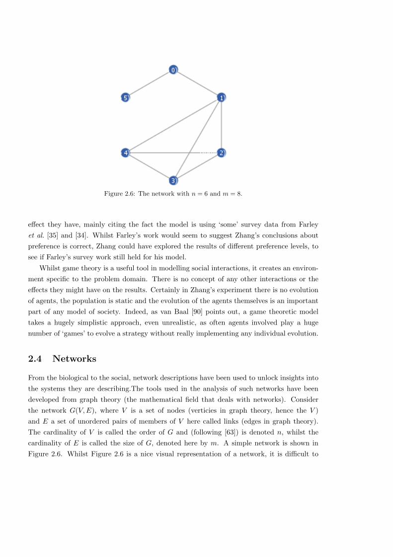
2.6 The network with n = 6 and m = 8 . . . . . . . . . . . . . . . . . . . . . . . . 14
2.7 A comparison of path lengths . . . . . . . . . . . . . . . . . . . . . . . . . . . 17
2.8 The degree distribution . . . . . . . . . . . . . . . . . . . . . . . . . . . . . . 17
2.9 The network with p0 = 1 . . . . . . . . . . . . . . . . . . . . . . . . . . . . . . 18
2.10 A GIS representation of Ya↵o . . . . . . . . . . . . . . . . . . . . . . . . . . . 24
2.11 An example neighbourhood . . . . . . . . . . . . . . . . . . . . . . . . . . . . 25
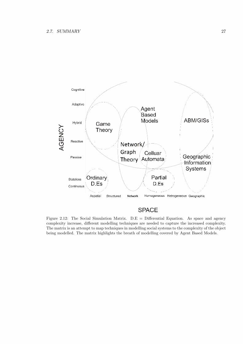
2.12 The Social Simulation Matrix . . . . . . . . . . . . . . . . . . . . . . . . . . . 27
3.1 Schelling’s one dimensional Spatial Proximity Model . . . . . . . . . . . . . . 30
3.2 Schelling’s two dimensional Spatial Proximity Model . . . . . . . . . . . . . . 35
3.3 Spatial Proximity Model final configuration . . . . . . . . . . . . . . . . . . . 35
3.4 Spatial Proximity Model ‘random movement’ final configuration . . . . . . . . 36
3.5 Schelling’s Tolerance Schedule . . . . . . . . . . . . . . . . . . . . . . . . . . . 37
3.6 Schelling’s Bounded Neighbourhood Model . . . . . . . . . . . . . . . . . . . 40
3.7 Schelling’s Bounded Neighbourhood model setup . . . . . . . . . . . . . . . . 41
3.8 Schelling’s Bounded Neighbourhood model with limited ratios . . . . . . . . . 42
3.9 Schelling’s Tipping model diagram . . . . . . . . . . . . . . . . . . . . . . . . 43
3.10 Schelling’s second Tipping Model diagram . . . . . . . . . . . . . . . . . . . . 44
4.1 Sargent’s framework . . . . . . . . . . . . . . . . . . . . . . . . . . . . . . . . 51
4.2 The CoSMoS process . . . . . . . . . . . . . . . . . . . . . . . . . . . . . . . . 53
4.3 Static results of Schelling’s Bounded Neighbourhood Model . . . . . . . . . . 56
ix
x LIST OF FIGURES
4.4 Dynamic results of Schelling’s Bounded Neighbourhood Model . . . . . . . . 57
4.5 Dynamic results of Schelling’s Bounded Neighbourhood Model . . . . . . . . 58
4.6 Distributions of data to be analysed . . . . . . . . . . . . . . . . . . . . . . . 60
4.7 Distributions of further data to be analysed . . . . . . . . . . . . . . . . . . . 62
5.1 Tolerance schedule and its realisation . . . . . . . . . . . . . . . . . . . . . . . 64
5.2 Schelling’s process in developing the Bounded Neighbourhood Model . . . . . 64
5.3 Applying CoSMoS to Schelling’s Bounded Neighbourhood Model . . . . . . . 65
5.4 The straight line tolerance schedules of the W and B populations . . . . . . . 69
5.5 Movement rules for the W population moving in . . . . . . . . . . . . . . . . 74
5.6 Movement rules for the W population moving out . . . . . . . . . . . . . . . 75
5.7 Validating the simulation . . . . . . . . . . . . . . . . . . . . . . . . . . . . . 79
6.1 Applying CoSMoS to test the movement rule . . . . . . . . . . . . . . . . . . 82
6.2 Comparison of deterministic and random movement . . . . . . . . . . . . . . 85
6.3 Comparison of population flows . . . . . . . . . . . . . . . . . . . . . . . . . . 86
6.4 Cumulative frequency distribution of I . . . . . . . . . . . . . . . . . . . . . . 87
6.5 Selected flows . . . . . . . . . . . . . . . . . . . . . . . . . . . . . . . . . . . . 88
6.6 Cumulative frequency of I for di↵ering seeds. . . . . . . . . . . . . . . . . . . 90
7.1 An application of the CoSMoS process in testing the e↵ect of agents’ exact
knowledge . . . . . . . . . . . . . . . . . . . . . . . . . . . . . . . . . . . . . . 96
7.2 Comparison of the population colour maps . . . . . . . . . . . . . . . . . . . . 100
7.3 Comparison of the population flows . . . . . . . . . . . . . . . . . . . . . . . . 101
7.4 Comparing S = 75 and S = 50 . . . . . . . . . . . . . . . . . . . . . . . . . . 102
7.5 Comparing S = 25 and S = 10 . . . . . . . . . . . . . . . . . . . . . . . . . . 103
7.6 Comparison of the population flows for S = 75 and S = 50 . . . . . . . . . . . 104
7.7 Comparison of the population flows for S = 25 and S = 10 . . . . . . . . . . . 105
7.8 Comparison of the distribution of I for di↵ering values of S . . . . . . . . . . 106
7.9 Three dimensional flow of di↵erent seeds, from initial condition (25O, 50B). . 109
8.1 An application of the CoSMoS process in testing the e↵ect of agents’ instant
movement . . . . . . . . . . . . . . . . . . . . . . . . . . . . . . . . . . . . . . 112
8.2 Probability distributions . . . . . . . . . . . . . . . . . . . . . . . . . . . . . . 115
8.3 A colour map of the adapted segregation model . . . . . . . . . . . . . . . . . 118
8.4 The population flows of the adapted segregation model . . . . . . . . . . . . . 119
8.5 Colour map of the final population levels for F = 1 and F = 5 . . . . . . . . 121
LIST OF FIGURES xi
8.6 Colour map of the final population levels for F = 10 and F = 20 . . . . . . . 122
8.7 Population flows with F = 1 and F = 5 . . . . . . . . . . . . . . . . . . . . . 123
8.8 Population flows with F = 10 and F = 20 . . . . . . . . . . . . . . . . . . . . 124
8.9 Distibution of population runtimes for the di↵erent values of F . . . . . . . . 125
9.1 An application of the CoSMoS process to develop a network model . . . . . . 128
9.2 Translating Schelling’s Bounded Neighbourhood model as a network . . . . . 129
9.3 A simple run of the Platform Model . . . . . . . . . . . . . . . . . . . . . . . 132
9.4 Comparing the dynamic results of the network implementation . . . . . . . . 134
9.5 Adding a social network . . . . . . . . . . . . . . . . . . . . . . . . . . . . . . 135
9.6 Comparison of social networks and their resulting ms. . . . . . . . . . . . . . 137
9.7 An example run of the small world social network . . . . . . . . . . . . . . . . 139
9.8 The distributions of six social networks . . . . . . . . . . . . . . . . . . . . . 140
9.9 Comparing runtime distributions of di↵erent small world networks . . . . . . 141
9.10 Comparing runtime distributions of di↵erent random networks . . . . . . . . 142
9.11 Comparing neighbourhood network configurations . . . . . . . . . . . . . . . 143
9.12 Plot of M against ⇢ . . . . . . . . . . . . . . . . . . . . . . . . . . . . . . . . 147

xii LIST OF FIGURES
List of Tables
1.1 Examples of complexity . . . . . . . . . . . . . . . . . . . . . . . . . . . . . . 2
3.1 Techniques used by researchers modelling segregation . . . . . . . . . . . . . . 47
4.1 U test example data . . . . . . . . . . . . . . . . . . . . . . . . . . . . . . . . 59
6.1 Results from Chapter 6 . . . . . . . . . . . . . . . . . . . . . . . . . . . . . . 90
7.1 Results from Chapter 7 . . . . . . . . . . . . . . . . . . . . . . . . . . . . . . 107
8.1 Results from Chapter 8 . . . . . . . . . . . . . . . . . . . . . . . . . . . . . . 120
9.1 Results from Chapter 9 . . . . . . . . . . . . . . . . . . . . . . . . . . . . . . 145
xiii

xiv LIST OF TABLES

Acknowledgements
I would like to thank my supervisors, Susan Stepney, Leo Caves and Emma Uprichard for
their continual guidance and support. In addition thanks to Dan Franks for some fruitful
discussions about networks, and Simon Poulding for help with the statistical analysis. Finally
thanks to my family for their endless help, support and patience.
xv

xvi ACKNOWLEDGEMENTS

Authour’s declaration
I declare that this thesis is a presentation of original work and I am the sole author. This
work has not previously been presented for an award at this, or any other, University. All
sources are acknowledged as References.
xvii

xviii AUTHOUR’S DECLARATION
Chapter 1
Introduction
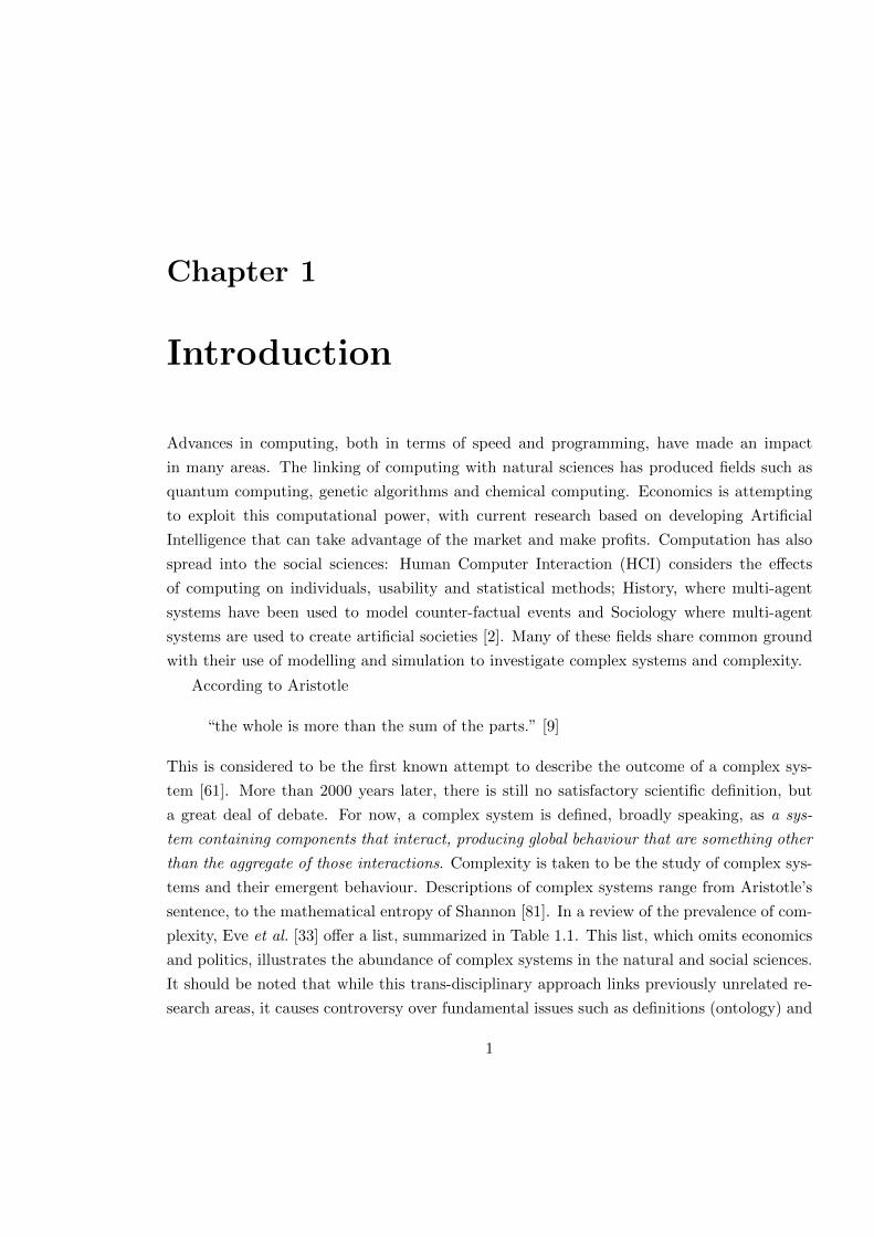
Advances in computing, both in terms of speed and programming, have made an impact
in many areas. The linking of computing with natural sciences has produced fields such as
quantum computing, genetic algorithms and chemical computing. Economics is attempting
to exploit this computational power, with current research based on developing Artificial
Intelligence that can take advantage of the market and make profits. Computation has also
spread into the social sciences: Human Computer Interaction (HCI) considers the e↵ects
of computing on individuals, usability and statistical methods; History, where multi-agent
systems have been used to model counter-factual events and Sociology where multi-agent
systems are used to create artificial societies [2]. Many of these fields share common ground
with their use of modelling and simulation to investigate complex systems and complexity.
According to Aristotle
“the whole is more than the sum of the parts.” [9]
This is considered to be the first known attempt to describe the outcome of a complex sys-
tem [61]. More than 2000 years later, there is still no satisfactory scientific definition, but
a great deal of debate. For now, a complex system is defined, broadly speaking, as a sys-
tem containing components that interact, producing global behaviour that are something other
than the aggregate of those interactions. Complexity is taken to be the study of complex sys-
tems and their emergent behaviour. Descriptions of complex systems range from Aristotle’s
sentence, to the mathematical entropy of Shannon [81]. In a review of the prevalence of com-
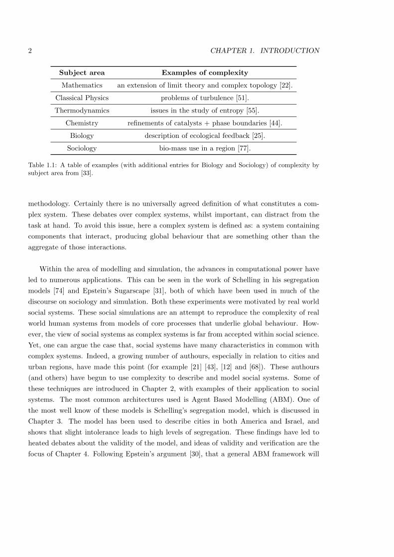
plexity, Eve et al. [33] o↵er a list, summarized in Table 1.1. This list, which omits economics
and politics, illustrates the abundance of complex systems in the natural and social sciences.
It should be noted that while this trans-disciplinary approach links previously unrelated re-
search areas, it causes controversy over fundamental issues such as definitions (ontology) and
1
2 CHAPTER 1. INTRODUCTION
Subject area Examples of complexity
Mathematics an extension of limit theory and complex topology [22].
Classical Physics problems of turbulence [51].
Thermodynamics issues in the study of entropy [55].
Chemistry refinements of catalysts + phase boundaries [44].
Biology description of ecological feedback [25].
Sociology bio-mass use in a region [77].
Table 1.1: A table of examples (with additional entries for Biology and Sociology) of complexity bysubject area from [33].
methodology. Certainly there is no universally agreed definition of what constitutes a com-
plex system. These debates over complex systems, whilst important, can distract from the
task at hand. To avoid this issue, here a complex system is defined as: a system containing
components that interact, producing global behaviour that are something other than the
aggregate of those interactions.
Within the area of modelling and simulation, the advances in computational power have
led to numerous applications. This can be seen in the work of Schelling in his segregation
models [74] and Epstein’s Sugarscape [31], both of which have been used in much of the
discourse on sociology and simulation. Both these experiments were motivated by real world
social systems. These social simulations are an attempt to reproduce the complexity of real
world human systems from models of core processes that underlie global behaviour. How-
ever, the view of social systems as complex systems is far from accepted within social science.
Yet, one can argue the case that, social systems have many characteristics in common with
complex systems. Indeed, a growing number of authours, especially in relation to cities and
urban regions, have made this point (for example [21] [43], [12] and [68]). These authours
(and others) have begun to use complexity to describe and model social systems. Some of
these techniques are introduced in Chapter 2, with examples of their application to social
systems. The most common architectures used is Agent Based Modelling (ABM). One of
the most well know of these models is Schelling’s segregation model, which is discussed in
Chapter 3. The model has been used to describe cities in both America and Israel, and
shows that slight intolerance leads to high levels of segregation. These findings have led to
heated debates about the validity of the model, and ideas of validity and verification are the
focus of Chapter 4. Following Epstein’s argument [30], that a general ABM framework will
3
emerge from individual frameworks, the Complex System Modelling and Simulation (CoS-
MoS) process is applied to Schelling’s model. The CoSMoS process (discussed in Section 4.3)
has successfully developed valid simulations of complex systems. In a novel application, the
process is applied to Schelling’s Bounded Neighbourhood Model. The development of a valid
simulation of Schelling’s Bounded Neighbourhood Model is described in Chapter 5. Once val-
idated, the simulation is used to test Schelling’s ordered movement rule, the work is presented
in Chapter 6. Following the CoSMoS process, the results from the experiment lead to more
questions about the model. From this three assumptions are examined: Chapter 7 explores
the e↵ects of agents’ complete knowledge of the system; Chapter 8 restricts the movement of
the agents; whilst Chapter 9 recasts the model as a network and introduces a social network.
A summary of the results and contributions of the thesis, as well as some conclusions and
further work, are presented in Chapter 10.

4 CHAPTER 1. INTRODUCTION
Chapter 2
Modelling Social Systems
Although there is disagreement about the structural aspects of social systems, a minimal
requirement is the interaction of two organisms [100]. There is agreement that social systems
have many characteristics in keeping with complex systems [73]. From this stems the belief
that the tools and techniques of complexity can be applied to social systems. Although the
field of complexity could be seen to have strong links to sociology [21], the ideas are still
far from accepted by many in the social sciences. Authours such as Sawyer [73], Byrne [21],
Fossett [37] and Walby [95] are suggesting that the tools of complexity o↵er a great deal to
social science. Some of the tools are now presented, with brief examples of their application
to social systems.
2.1 Di↵erential Equations
Di↵erential Equations are at the heart of mathematical physics and are a significant motiva-
tion for mathematical analysis [82]. Di↵erential equations involve the relationship between
infinitesimal changes of independent variables (such as time) and the dependent variables
such as temperature. In the simplest case, given a ‘smooth’ function y = f(x), its derivative
f 0(x) = dy/dx can be interpreted as the rate of change of y with respect to x. Many of the
general laws of nature, such as physics, chemistry, biology and astronomy, can be expressed
in this language. In the physical sciences the equations are developed from a deep and precise
understanding of the phenomena being studied. It is e↵ective where the constituent entities
are homogeneous, deterministic and smooth (at least statistically).
The Italian mathematician Volterra, known for his work on integral equations, used dif-
ferential equations to model biological systems [92]. This mathematical biology led Alfred
Lotka to theorise that natural selection was a struggle for available energy. Those organisms
5
6 CHAPTER 2. MODELLING SOCIAL SYSTEMS
that capture and use energy most e�ciently are the ones that prosper. (It is interesting that
he suggested the switch in society from solar to non-renewable energy would pose a funda-
mental challenge [5]). Applying these ideas of e�ciency to animal populations led to the
development of the Lotka-Volterra predator prey model. The equations model the growth
and decline of two populations, one predator (often referred to as foxes) and one prey (often
rabbits). Let R(t) and F (t) represent the number of rabbits and foxes respectively that are
alive at time t, then the Lotka-Volterra model [86] is:
dR
dt= aR� bRF,
dF
dt= eRF � cF,
where a is the natural growth rate of rabbits in the absence of predation (foxes), b is the death
rate per encounter of rabbits due to predation (foxes), c is the natural death rate of foxes in
the absence of food (rabbits), and e is the e�ciency of turning predated rabbits into fox’s
o↵spring. The equations are part of a family of models known as logistic growth equations,
other types include the parasitic model and the competition model. The parameters selected
are considered to be the most important aspects of the system being analysed. Certainly
birth and death rates are the most important factor in population size and these are clearly
a↵ected by the presence (or absence) of food. In the model the number of encounters between
the two groups is found to be proportional to the number of rabbits times the number of
foxes. This would seem to imply there is no spatial segregation of the populations as they
appear to consistently encounter each other. Despite their relative simplicity these equations
have been successful at modelling pairs of populations such as lynxs and hares in the Hudson
Bay [54] and, according to Kau↵mann [50, p210], arctic foxes and hares as well as commercial
fishing in the Adriatic.
In an influential paper, Hosler et al. [48] used di↵erential equations to model the collapse
of the Mayan civilization between 750 - 900AD. Basing their work on the anthropologi-
cal theory put forward by Willey and Shimkin [101], they developed a model based on a
deviation-amplifying feedback loop, between the increasing ritual and public building. This
enhanced the prestige of the elite, led to the consequent decline in food production, which
was considered demeaning [48]. These and other elements, of the social and economic systems
that made up the society, were quantified. From these, specified recurrence equations1 were
1“A recurrence equation (or di↵erence equation) is the discrete analog of a di↵erential equation. A dif-ference equation involves an integer function f(n) in a form like f(n) � f(n � 1) = g(n) where g issome integer function. This equation is the discrete analog of the first-order ordinary di↵erential equationf 0(x) = g(x).” [59].
2.1. DIFFERENTIAL EQUATIONS 7
chosen, to determine their interacting behaviour over time. The model produced showed a
collapse, and further, that di↵erent behaviours from the ruling elite, could have postponed
the collapse (although not prevent it). However, it is important to note that, in his critique,
Gilbert [43, p42] points out this model completely ignores some, seemingly important, fac-
tors such as interactions with other tribes, warfare and spatial factors. Indeed later studies
showed the Mayan ‘collapse’ was less suddenm and pointed towards a more gradual shift
of dominance from one part of the region to another. This result exemplifies the danger of
producing models with inaccurate data, and without careful consideration of the techniques
being used. It certainly shows that, when modelling complex systems, even the ‘correct’ result
can sometimes be ‘wrong’. Often di↵erential equations, or some variation such as di↵erence
equations, are more than adequate for simulating dynamical systems. But, if the system be-
ing measured is non-linear, even the smallest of variations in the initial settings can have an
exponential e↵ect on the outcome (sensitivity to initial data or ‘Butterfly E↵ect [86]). This
problem has become well known and can be traced back to Lorenz’s attempts to model the
weather using a computer simulation based on the following simple system of three ordinary
coupled di↵erential equations that describe the relevant atmospheric physics [86].
dx
dt= �(y � x)
dy
dt= x(�� z)� y
dz
dt= xy � �z,
where �,�,� > 0 are physical constants.2 After Lorenz repeated his calculations from an
earlier data point, he noticed significant deviations developed in time even though calculation
were restarted from the exact same point in the plot. This was the origin of the familiar
Butterfly E↵ect, as apparently insignificant rounding errors correspond to the e↵ect that the
motion of a butterfly’s wings could have on the weather.
Di↵erential equations are often used to investigate systems in the natural sciences. How-
ever they are unable to capture individual behaviours of members of a population being
modelled. Additionally they are only able to incorporate spatial aspects of the system by
2for the interested reader � is the Prandtl number which “. . . is a dimensionless number approximating theratio of momentum di↵usivity (kinematic viscosity) and thermal di↵usivity. It is named after the Germanphysicist Ludwig Prandtl” [97]. � is the Rayleigh number which “. . . is a dimensionless number associatedwith buoyancy driven flow (also known as free convection or natural convection). When the Rayleigh numberis below the critical value for that fluid, heat transfer is primarily in the form of conduction; when it exceedsthe critical value, heat transfer is primarily in the form of convection” [98].
8 CHAPTER 2. MODELLING SOCIAL SYSTEMS
introducing further variables. This leads to more intractable partial di↵erential equations.
Moreover, while models of complex systems using di↵erential equations can be accurate over
small timescales, their nature means that any real long term predictions su↵er from expo-
nential error rates. Parameters selected for modelling in the natural sciences are usually very
simplistic and are, perhaps, chosen more for mathematical simplicity. For example in the
predator-prey model, the parameter that relates the food obtained to the number of o↵spring
is hardly a realistic representation. The o↵spring are the result of far more complex inter-
actions than just the amount of food available. Introducing more parameters to make the
simulation more realistic would obviously make the equations more complicated. Moreover
some natural aspects such as hunting or escape strategies cannot be incorporated in a simple
way into numerical equations. There is no way, at present, of introducing modifications to
the environment; the results of external changes can only be seen in terms of population
numbers. Drogoul and Ferber [27] point this out, arguing that, with numerical modelling,
the hunting/feeding process can only be represented by the volume of available prey, and
the probability of the predator finding the prey. Rather than describing the behaviour of
the predators/prey, it can only quantify the relation between the numbers involved. Finally,
numerical simulations are unable to cope with qualitative data, such as the relation between
a stimulus and the behaviour of an individual, which are well beyond the scope of analytical
equations and numerical simulations [27]. Perhaps most important, there seems to be no way
of capturing the evolution of ‘emergent’ behaviour or structure. Whilst modelling complex
systems using di↵erential equations o↵ers a reasonable representation at a population level,
it is clear that there are limitations that need to be taken into consideration. Most impor-
tantly, dealing with qualitative data is proving intractable in models for the natural and
social sciences. Nevertheless, despite this, some simpler complex systems can be represented
by a relatively small number of key variables.
2.2 Cellular Automata
Cellular Automata (CAs) were developed by von Neumann and Ulam [94] in the 1940s.
In collaboration with another mathematician Ulam, von Neumann had been searching for
logical solutions to the complexity of natural growth [99]. Von Neumann demonstrated that,
on a two dimensional lattice grid, particular patterns of cells, with 29 states and specific
state transitions, could self-replicate. It was discoverd that simple rules, governing state
transitions, can create a variety of unexpected behaviours. Wolfram [104] used a simple form
of CA, what he called an ‘elementary cellular automata’. Elementary CAs have two possible
values for each cell (0 or 1), and rules that depend only on the values of the cells directly
2.2. CELLULAR AUTOMATA 9
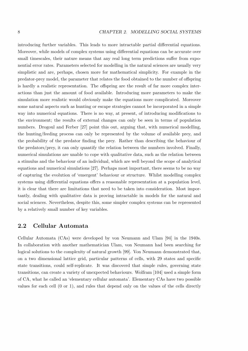
Figure 2.1: Wolfram’s binary representation of 30
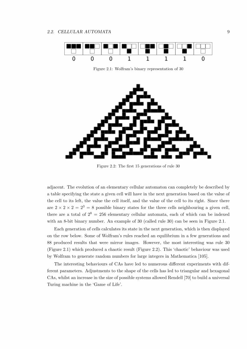
Figure 2.2: The first 15 generations of rule 30
adjacent. The evolution of an elementary cellular automaton can completely be described by
a table specifying the state a given cell will have in the next generation based on the value of
the cell to its left, the value the cell itself, and the value of the cell to its right. Since there
are 2 ⇥ 2 ⇥ 2 = 23 = 8 possible binary states for the three cells neighbouring a given cell,
there are a total of 28 = 256 elementary cellular automata, each of which can be indexed
with an 8-bit binary number. An example of 30 (called rule 30) can be seen in Figure 2.1.
Each generation of cells calculates its state in the next generation, which is then displayed
on the row below. Some of Wolfram’s rules reached an equilibrium in a few generations and
88 produced results that were mirror images. However, the most interesting was rule 30
(Figure 2.1) which produced a chaotic result (Figure 2.2). This ‘chaotic’ behaviour was used
by Wolfram to generate random numbers for large integers in Mathematica [105].
The interesting behaviours of CAs have led to numerous di↵erent experiments with dif-
ferent parameters. Adjustments to the shape of the cells has led to triangular and hexagonal
CAs, whilst an increase in the size of possible systems allowed Rendell [70] to build a universal
Turing machine in the ‘Game of Life’.
10 CHAPTER 2. MODELLING SOCIAL SYSTEMS
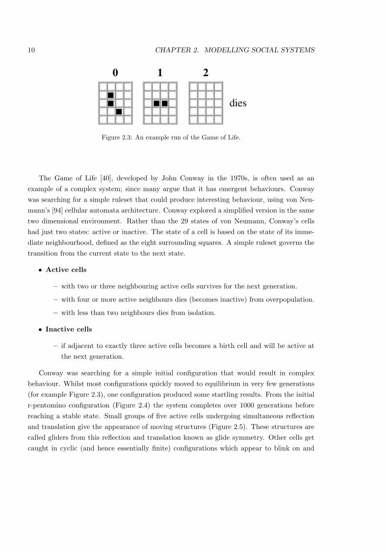
Figure 2.3: An example run of the Game of Life.
The Game of Life [40], developed by John Conway in the 1970s, is often used as an
example of a complex system; since many argue that it has emergent behaviours. Conway
was searching for a simple ruleset that could produce interesting behaviour, using von Neu-
mann’s [94] cellular automata architecture. Conway explored a simplified version in the same
two dimensional environment. Rather than the 29 states of von Neumann, Conway’s cells
had just two states: active or inactive. The state of a cell is based on the state of its imme-
diate neighbourhood, defined as the eight surrounding squares. A simple ruleset governs the
transition from the current state to the next state.
• Active cells
– with two or three neighbouring active cells survives for the next generation.
– with four or more active neighbours dies (becomes inactive) from overpopulation.
– with less than two neighbours dies from isolation.
• Inactive cells
– if adjacent to exactly three active cells becomes a birth cell and will be active at
the next generation.
Conway was searching for a simple initial configuration that would result in complex
behaviour. Whilst most configurations quickly moved to equilibrium in very few generations
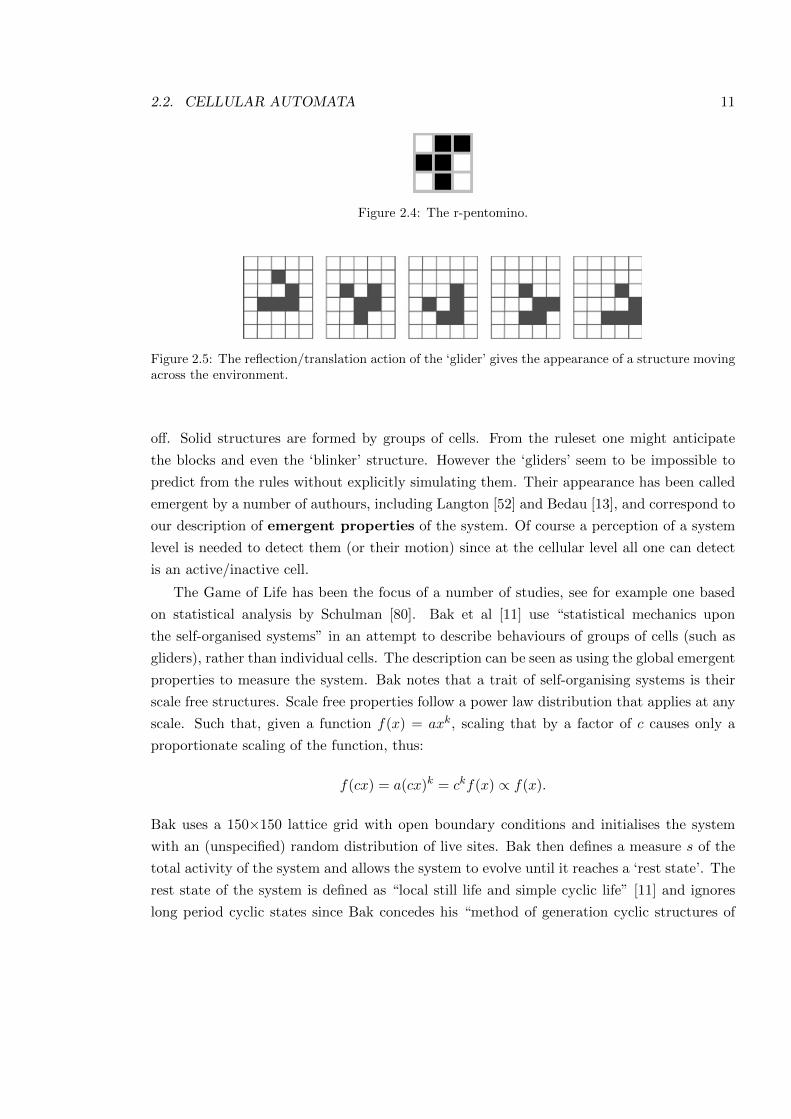
(for example Figure 2.3), one configuration produced some startling results. From the initial
r-pentomino configuration (Figure 2.4) the system completes over 1000 generations before
reaching a stable state. Small groups of five active cells undergoing simultaneous reflection
and translation give the appearance of moving structures (Figure 2.5). These structures are
called gliders from this reflection and translation known as glide symmetry. Other cells get
caught in cyclic (and hence essentially finite) configurations which appear to blink on and
2.2. CELLULAR AUTOMATA 11
Figure 2.4: The r-pentomino.
Figure 2.5: The reflection/translation action of the ‘glider’ gives the appearance of a structure movingacross the environment.
o↵. Solid structures are formed by groups of cells. From the ruleset one might anticipate
the blocks and even the ‘blinker’ structure. However the ‘gliders’ seem to be impossible to
predict from the rules without explicitly simulating them. Their appearance has been called
emergent by a number of authours, including Langton [52] and Bedau [13], and correspond to
our description of emergent properties of the system. Of course a perception of a system
level is needed to detect them (or their motion) since at the cellular level all one can detect
is an active/inactive cell.
The Game of Life has been the focus of a number of studies, see for example one based
on statistical analysis by Schulman [80]. Bak et al [11] use “statistical mechanics upon
the self-organised systems” in an attempt to describe behaviours of groups of cells (such as
gliders), rather than individual cells. The description can be seen as using the global emergent
properties to measure the system. Bak notes that a trait of self-organising systems is their
scale free structures. Scale free properties follow a power law distribution that applies at any
scale. Such that, given a function f(x) = axk, scaling that by a factor of c causes only a
proportionate scaling of the function, thus:
f(cx) = a(cx)k = ckf(x) / f(x).
Bak uses a 150⇥150 lattice grid with open boundary conditions and initialises the system
with an (unspecified) random distribution of live sites. Bak then defines a measure s of the
total activity of the system and allows the system to evolve until it reaches a ‘rest state’. The
rest state of the system is defined as “local still life and simple cyclic life” [11] and ignores
long period cyclic states since Bak concedes his “method of generation cyclic structures of
12 CHAPTER 2. MODELLING SOCIAL SYSTEMS
long period are extremely rare and essentially never encountered” (Bak does not define what
the length of a long period is). Once the system is at rest, Bak perturbs it (without saying
what form the perturbation takes) and measures the activity that arises. This activity s is
the cumulative number of ‘births’ and ‘deaths’ from the initial rest state to the next rest
state. By averaging 40,000 such perturbations Bak finds that, not only does the distribution
of the activity of the system D(s) follow a power law D(s) / s�⌧ for ⌧ ⇡ 1.4, but so does the
distribution of the duration of the perturbations, D(T ) / T�b for b ⇡ 1.6 [11]. By ignoring
the low level interactions and instead focusing on the emergent behaviour of the system, Bak
is able to neatly side step having to track a possibly exponentially growing number of micro-
states. Since each cell can have two possible states n cells need to consider 2n possible states,
this means the possibles number of states for Bak’s experimental setup is 222500. The problem
is akin to the gas laws, whereby, whilst it is possible to work out the temperature, one could
never know the individual velocities of the molecules. So Bak et al. resort to measuring
the emergent properties rather than calculating individual cell positions and states. The
complexity the Game of Life produces from such simple rules o↵ers the possibility that, some
of the complexities of social interaction could be reduced to a few simple rules.
2.3 Game Theory
Game theory is a well known field of mathematics and was introduced by John von Neu-
mann and Oskar Morgenstern in their influential book “Theory of Games and Economic
behaviour” [93]. Game theory is the formal study of interactions between ‘goal-oriented’
agents and the strategic scenarios that arise in these settings. Further details can be found
in von Neumann’s book [93]. However, briefly, players interact through games of chance.
Their strategies are the executions of choices, based on a payo↵ and probability. Players
work towards maximizing their payo↵s by assuming all players will be doing the same and
thus attempting to develop a ‘best response’ to a rational choice.
A famous example of modelling using game theory is the prisoners’ dilemma. In this
problem two players (A and B) face a choice of betraying or co-operating. If both choose to
co-operate their payo↵ is 2, if they both betray the payo↵ is 1. The dilemma comes from
the fact that if one player betrays whilst the other co-operates the betraying player gets
a payo↵ of 3 whilst the co-operator gets nothing. Consider player A: if B co-operates, A
does better by betraying (3) than cooperating (2); if B betrays, A does better by betraying
than co-operating (0). Therefore, whatever happens, the best response for both players is to
betray, even though they would both be better o↵ if they both co-operated.
2.3. GAME THEORY 13
Zhang [109] uses Game Theory to model Schelling’s Bounded Neighbourhood Model. His
model is a lattice graph with periodic boundary conditions (i.e a torus), where each vertex
is a residential location. Any location i has H neighbouring vertices, where H is a fixed
integer. So that H = 4 would be a von Neumann neighbourhood and H = 8 is a Moore
neighbourhood. Pi is the price of location i, Wi the number of White neighbours and Bi the
number of Black neighbours. Zhang assumes all the agents earn an identical income Y, since
he claims that “even if each person i earns a di↵erent Yi, all results remain the same” [108].
The price Pi is determined by a simplified market mechanism whereby prices respond to
demand, more demand implies higher prices, so that Pi = Bi +Wi. From this Zhang is able
to define a utility of a White agent as Uwi = Y +⇡Wi�Pi = Y +(⇡�1)Wi�Bi where ⇡ > 0.
A positive value of ⇡ implies the more White neighbours a White agent has the happier the
agent is. Letting ✓ = ⇡ � 1 > �1 gives
Uwi = Y + ✓Wi �Bi.
Zhang now assumes Blacks care only about price at location j giving them a utility,
Ubj = Y � Pj
= Y �Wj �Bj .
From this utility Zhang makes a proposition:
If Blacks are colour-neutral and Whites have a slight preference for like-colour
neighbours, then, in the long run: (i) residential segregation is observed most of
the time; (ii) the rate of vacancy is higher in Black neighbourhoods than in White
neighbourhoods; and (iii) Whites pay more than Blacks do for equivalent housing.
Zhang’s model points to this proposition, since Whites would be unwilling to move to a black
neighbourhood, whereas blacks would have no problem moving. Although Zhang introduces
a bounded rationality, in that agents will sometimes make utility decreasing moves, the e↵ect
is negated over the time periods he uses. The erroneous moves are eventually outweighed
by rational movement. Zhang’s Pi equation assumes location i is occupied because Zhang
believes it odd that i commands a di↵erent price before and after an agent moves in. No
evidence to support this assumption is given (and if one considers a property that has been
vacant for a long period of time, the price could increase if it became occupied). It is possible
that Zhang would consider the change in price to be led by the market as a whole rather than
an individual in the market. Additionally the model uses rental housing market data to define
the pricing mechanism. Zhang fails to experiment with the preference parameters to see the
14 CHAPTER 2. MODELLING SOCIAL SYSTEMS
Figure 2.6: The network with n = 6 and m = 8.
e↵ect they have, mainly citing the fact the model is using ‘some’ survey data from Farley
et al. [35] and [34]. Whilst Farley’s work would seem to suggest Zhang’s conclusions about
preference is correct, Zhang could have explored the results of di↵erent preference levels, to
see if Farley’s survey work still held for his model.
Whilst game theory is a useful tool in modelling social interactions, it creates an environ-
ment specific to the problem domain. There is no concept of any other interactions or the
e↵ects they might have on the results. Certainly in Zhang’s experiment there is no evolution
of agents, the population is static and the evolution of the agents themselves is an important
part of any model of society. Indeed, as van Baal [90] points out, a game theoretic model
takes a hugely simplistic approach, even unrealistic, as often agents involved play a huge
number of ‘games’ to evolve a strategy without really implementing any individual evolution.
2.4 Networks
From the biological to the social, network descriptions have been used to unlock insights into
the systems they are describing.The tools used in the analysis of such networks have been
developed from graph theory (the mathematical field that deals with networks). Consider
the network G(V,E), where V is a set of nodes (verticies in graph theory, hence the V )
and E a set of unordered pairs of members of V here called links (edges in graph theory).
The cardinality of V is called the order of G and (following [63]) is denoted n, whilst the
cardinality of E is called the size of G, denoted here by m. A simple network is shown in
Figure 2.6. Whilst Figure 2.6 is a nice visual representation of a network, it is di�cult to
2.4. NETWORKS 15
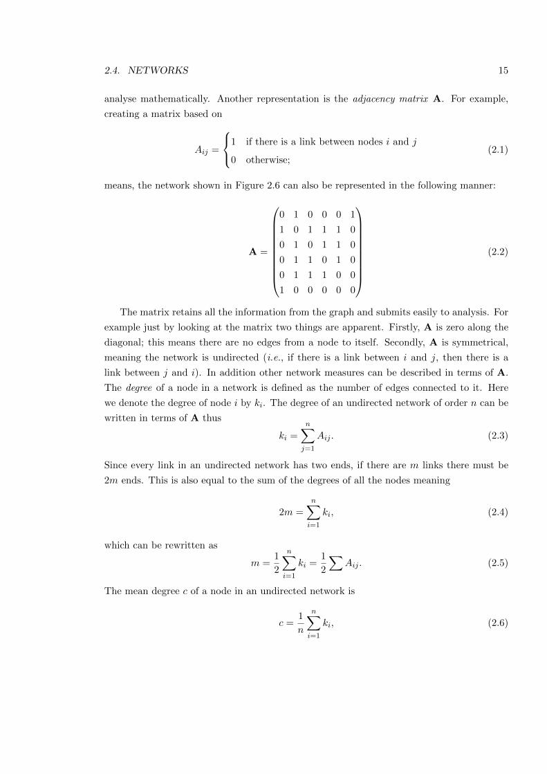
analyse mathematically. Another representation is the adjacency matrix A. For example,
creating a matrix based on
Aij =
8<
:1 if there is a link between nodes i and j
0 otherwise;(2.1)
means, the network shown in Figure 2.6 can also be represented in the following manner:
A =
0
BBBBBBBBB@
0 1 0 0 0 1
1 0 1 1 1 0
0 1 0 1 1 0
0 1 1 0 1 0
0 1 1 1 0 0
1 0 0 0 0 0
1
CCCCCCCCCA
(2.2)
The matrix retains all the information from the graph and submits easily to analysis. For
example just by looking at the matrix two things are apparent. Firstly, A is zero along the
diagonal; this means there are no edges from a node to itself. Secondly, A is symmetrical,
meaning the network is undirected (i.e., if there is a link between i and j, then there is a
link between j and i). In addition other network measures can be described in terms of A.
The degree of a node in a network is defined as the number of edges connected to it. Here
we denote the degree of node i by ki. The degree of an undirected network of order n can be
written in terms of A thus
ki =nX
j=1
Aij . (2.3)
Since every link in an undirected network has two ends, if there are m links there must be
2m ends. This is also equal to the sum of the degrees of all the nodes meaning
2m =nX
i=1
ki, (2.4)
which can be rewritten as
m =1
2
nX
i=1
ki =1
2
XAij . (2.5)
The mean degree c of a node in an undirected network is
c =1
n
nX
i=1
ki, (2.6)
16 CHAPTER 2. MODELLING SOCIAL SYSTEMS
which, when combined with equation (2.3), gives
c =2m
n. (2.7)
Applying this to the example network m = 8 and n = 6,
c =2(8)
6=
8
3. (2.8)
The maximum possible connections available to a network (with n � 2) is 12n(n � 1). This
can be used to calculate the density
⇢ =2m
n(n� 1)=
c
n� 1. (2.9)
The range of ⇢ is strictly 0 ⇢ 1. Applying this to the example network (Figure 2.6)
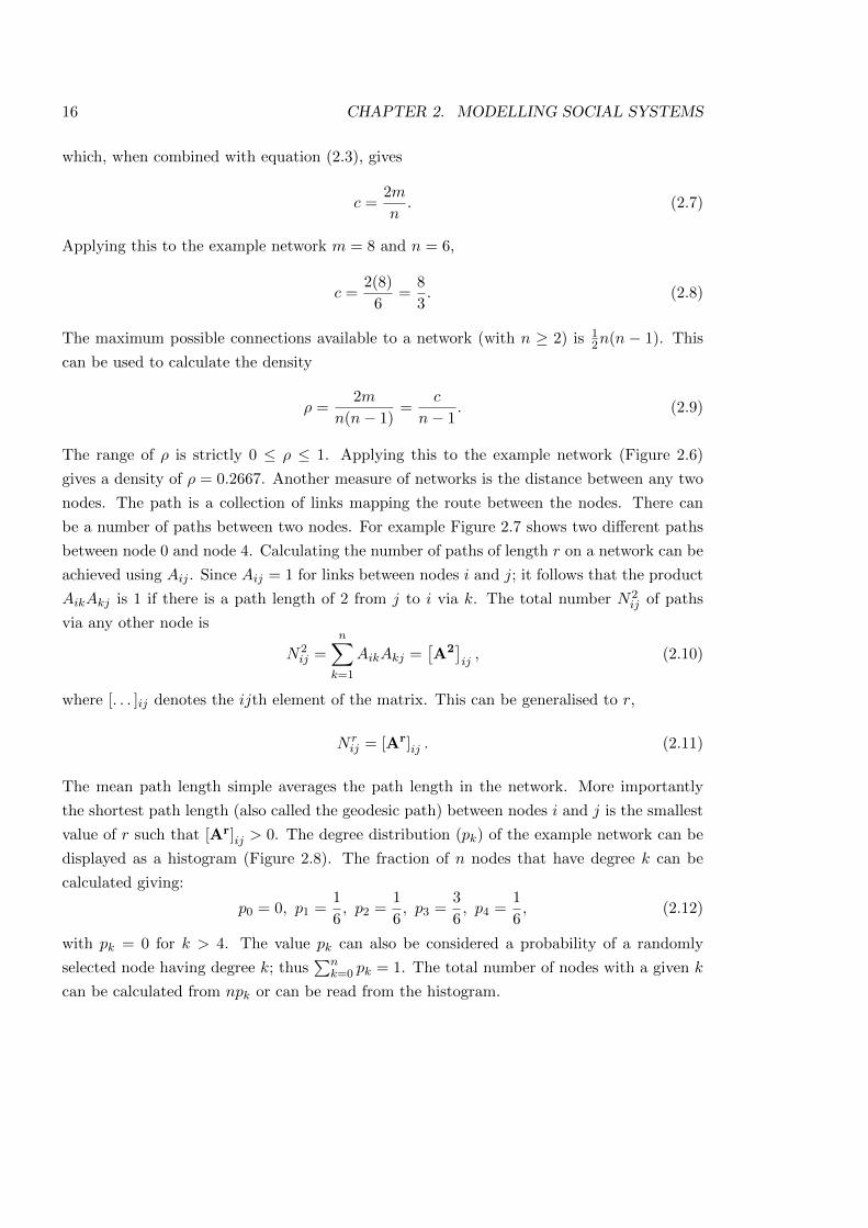
gives a density of ⇢ = 0.2667. Another measure of networks is the distance between any two
nodes. The path is a collection of links mapping the route between the nodes. There can
be a number of paths between two nodes. For example Figure 2.7 shows two di↵erent paths
between node 0 and node 4. Calculating the number of paths of length r on a network can be
achieved using Aij . Since Aij = 1 for links between nodes i and j; it follows that the product
AikAkj is 1 if there is a path length of 2 from j to i via k. The total number N2ij of paths
via any other node is
N2ij =
nX
k=1
AikAkj =⇥A2
⇤ij, (2.10)
where [. . . ]ij denotes the ijth element of the matrix. This can be generalised to r,
N rij = [Ar]ij . (2.11)
The mean path length simple averages the path length in the network. More importantly
the shortest path length (also called the geodesic path) between nodes i and j is the smallest
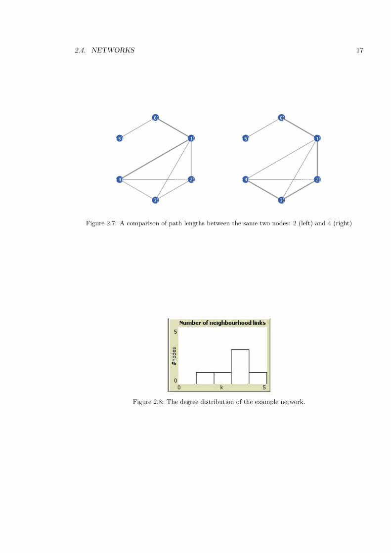
value of r such that [Ar]ij > 0. The degree distribution (pk) of the example network can be
displayed as a histogram (Figure 2.8). The fraction of n nodes that have degree k can be
calculated giving:
p0 = 0, p1 =1
6, p2 =
1
6, p3 =
3
6, p4 =
1
6, (2.12)
with pk = 0 for k > 4. The value pk can also be considered a probability of a randomly
selected node having degree k; thusPn
k=0 pk = 1. The total number of nodes with a given k
can be calculated from npk or can be read from the histogram.
2.4. NETWORKS 17
Figure 2.7: A comparison of path lengths between the same two nodes: 2 (left) and 4 (right)
Figure 2.8: The degree distribution of the example network.
18 CHAPTER 2. MODELLING SOCIAL SYSTEMS
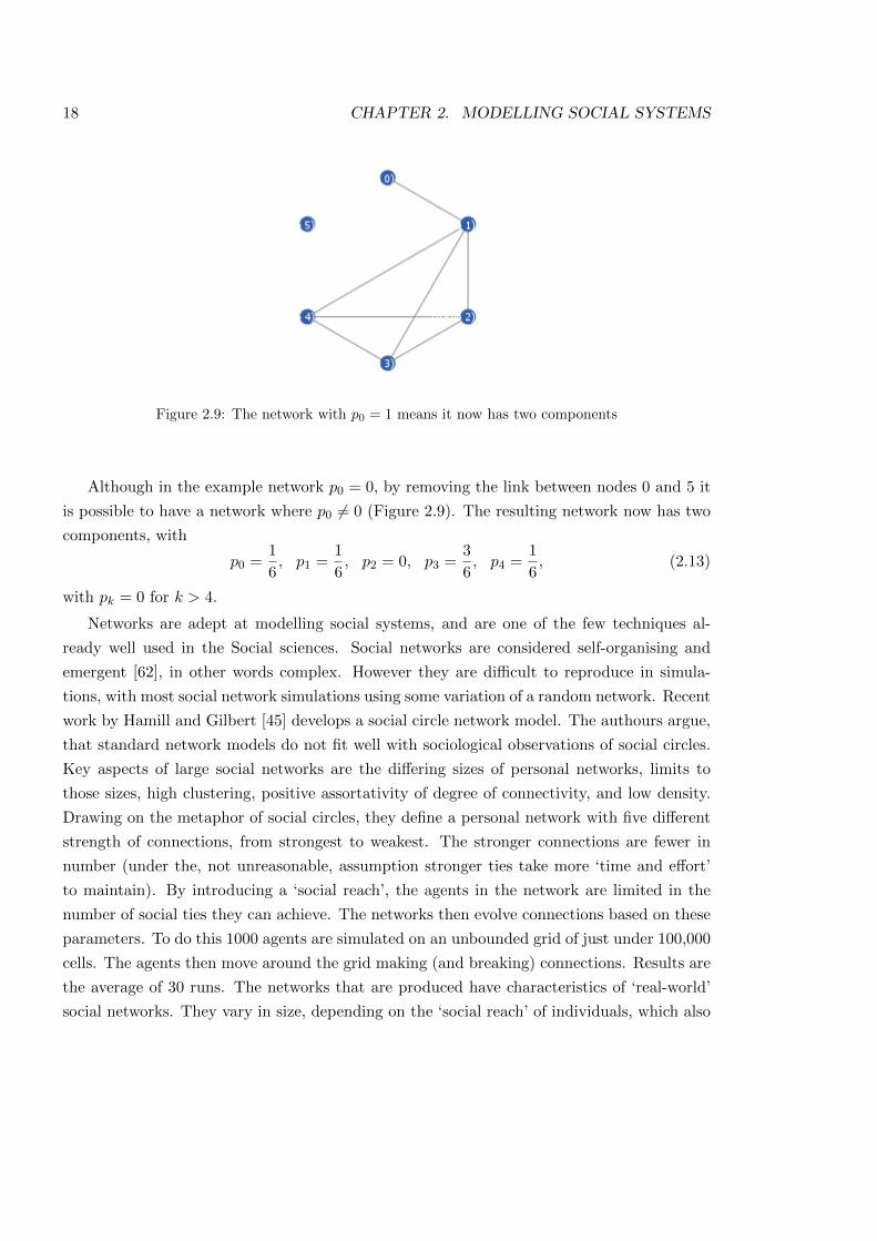
Figure 2.9: The network with p0 = 1 means it now has two components
Although in the example network p0 = 0, by removing the link between nodes 0 and 5 it
is possible to have a network where p0 6= 0 (Figure 2.9). The resulting network now has two
components, with
p0 =1
6, p1 =
1
6, p2 = 0, p3 =
3
6, p4 =
1
6, (2.13)
with pk = 0 for k > 4.
Networks are adept at modelling social systems, and are one of the few techniques al-
ready well used in the Social sciences. Social networks are considered self-organising and
emergent [62], in other words complex. However they are di�cult to reproduce in simula-
tions, with most social network simulations using some variation of a random network. Recent
work by Hamill and Gilbert [45] develops a social circle network model. The authours argue,
that standard network models do not fit well with sociological observations of social circles.
Key aspects of large social networks are the di↵ering sizes of personal networks, limits to
those sizes, high clustering, positive assortativity of degree of connectivity, and low density.
Drawing on the metaphor of social circles, they define a personal network with five di↵erent
strength of connections, from strongest to weakest. The stronger connections are fewer in
number (under the, not unreasonable, assumption stronger ties take more ‘time and e↵ort’
to maintain). By introducing a ‘social reach’, the agents in the network are limited in the
number of social ties they can achieve. The networks then evolve connections based on these
parameters. To do this 1000 agents are simulated on an unbounded grid of just under 100,000
cells. The agents then move around the grid making (and breaking) connections. Results are
the average of 30 runs. The networks that are produced have characteristics of ‘real-world’
social networks. They vary in size, depending on the ‘social reach’ of individuals, which also
2.5. AGENT BASED MODELLING 19
limits the size of the network. Overlapping social reaches cause high clustering, whilst the
movement of agents makes the networks dynamic. The social reach parameter seems to be
the key to the development of the networks. Whilst this is something that could lead to criti-
cism of simplicity, the authours note that their method simply “create[s] agent-based models
that represent empirical social networks with greater veracity than the standard network
models” [45, p91]. Certainly this is a useful method for developing ‘non-standard’ networks,
and further applications are likely. It is interesting to note, the method the authours use to
develop the network is Agent Based Modelling, which is one of the most used methods in
Social simulation.
2.5 Agent Based Modelling
Agent (or Individual) Based Modelling (ABM) is the use of a multi-agent environment archi-
tecture to model a system. The architecture is able to overcome some of the limitations of
previous techniques, by directly modelling individuals, and their interactions, in an environ-
ment. The agents are an abstract representation of the individual members of the population,
and the environment they interact with is an abstraction of their real world environment.
Therefore, modelling is done at a local scale, with the agent and its interactions with the
environment being modelled, rather than attempting to model the population as a whole. It
is defined by Wooldrige and Jennings [106] as
“An agent is a computer system that is situated in an environment and that is
capable of autonomous action in that environment to achieve its set objectives.”
According to Galan et al. [39], with agent-based modelling, the entities of the system are
represented explicitly and individually (but not necessarily accurately) in the model. The
limits of the entities in the target system, correspond to the limits of the agents in the model;
and the interactions between entities, correspond to the interactions of the agents in the
model. This abstract impression of an agent, means that it lends itself well to modelling a
number of di↵erent phenomena. Since the modelling of a system can now be done at a local
scale, it is believed that valid results will emerge from these individual processes.
There are those that argue agent models are non-mathematical and non-deductive, claim-
ing they lack the mathematical rigour of equation based analysis. Epstein [29] counters these
claims, arguing that every agent is a computer program and, as such, is computable by a
Turing machine (Turing computable). Since for every Turing machine there is a unique corre-
sponding, and equivalent, partial recursive function [47], in principle, one can cast any agent
based computational model as an explicit set of recursive functions. Although, in practice,
20 CHAPTER 2. MODELLING SOCIAL SYSTEMS
these might be extremely complex and di�cult to interpret they surely exist. This is a pow-
erful counter to the arguments that agent-based models are non-mathematical. As Epstein
points out, the non-deductiveness follows since recursive functions are computed determin-
istically from initial values. Given the nth (including the initial) state the nth+1st state is
computable, in a strictly mechanical and deterministic way, by recursion.
According to Epstein [31], Agent Based Modelling was first used by Schelling in his ‘Dy-
namical Models of Segregation’ [74] (although Schelling used di↵erent terminology). During
the first half of the 1990s researchers at the Santa Fe Institute, led by Joshua Epstein and
Robert Axtell, used agent architecture techniques and developed Sugarscape, an agent based
simulation, using a generative social science model [31]. The Santa Fe Institute has long
argued that ABMs are an excellent tool for modelling social phenomena, such as segrega-
tion. This is in no small part due to their suitability for modelling complex agents. ABMs
have been able to show how simple, and predictable, local interactions can generate familiar
global patterns, such as the di↵usion of information [31], emergence of norms [71], wealth
aggregation [31], segregation of populations [74] or participation in collective action [57]. Ep-
stein [29] talks of a generative social science and growing artificial societies from the bottom
up claiming “if you didn’t grow it, you didn’t explain its emergence.” Macy [57] gives strong
support to the generative views of Epstein, believing that ABMs o↵er theoretical leverage,
where the global patterns of interest can be seen to be more than, the aggregation of indi-
vidual attributes. Macy argues that emergent behaviours cannot be understood without a
bottom up dynamical model of the micro processes from individuals [57]. The simulation of
these individuals combines to give, what Sawyer calls, artificial societies, which he defines as
“a set of autonomous agents operating in parallel and communicating with each other” [73,
p2]. Sawyer argues these artificial societies will lead to an understanding of the mechanics
of micro-to-macro emergence, macro-to-micro causation and “the dialectic between social
emergence and social causation” [73, p8]. Macy hopes that ABMs could o↵er an alternative
approach for sociologists (and all social scientists), who have often modelled social processes
as interactions among variables [57]. Certainly ABMs seem to o↵er an excellent way to
model social systems. Schelling [74] used an ABM consisting of coins and a checkers board
to explore the e↵ects of individual preference on global segregation (the experiment is ex-
plored in full in section 3). His conclusions generated huge interest and some controversy
with sociologists such as Massey [58] and Yinger [107] criticising its simplistic nature. Even
so, Schelling’s models of segregation have become well known within the social simulation
community, precisely because they provide alternative modes of exploring issues, more com-
monly investigated using traditional statistical analysis. The apparent ease of modelling using
ABMs, most notably by Epstein [29] and the Santa Fe Institute, but also by Gilbert [43],
2.5. AGENT BASED MODELLING 21
Sawyer [73] and others, has led to an explosion of ABMs modelling social interaction. This
is well documented by both Railsback [69] and Nikolai and Madey [64] who identify over 50
current ABM platforms. However for all these platforms there is no universal approach to
this technique. Epstein believes a framework will emerge over time, as these many approaches
merge and are refined [30].
In the mean time, Laurie and Jaggie [53] use ABM techniques to explore some of the
e↵ects of changing the values of parameters selected by Schelling. They suggest most work
on Schelling’s models has focused on the preferences (p) of agents (defined in Section ?? as
⌧). Although Laurie and Jaggie use p, their main focus is on the neighbourhood of agents,
up to a distance of R, calling this parameter an agent’s vision. The environment consists
of an N ⇥ N square array, with periodic boundary conditions. This creates a society on
an edgeless torus rather than a square grid which, they argue, suppresses possible boundary
e↵ects. They then propose two more parameters: c for concentration of the minority race
and v, for the concentration of vacant residences. The system is initialised with N = 50,
whilst v is randomly initialised so that (1 � v)N2 sites are occupied by c(1 � v)N2 Blacks,
and (1 � c)(1 � v)N2 Whites. Since they are only interested in the e↵ect of R, they set
c = 0.5, so that the number of Blacks is equal to the number of Whites. At each iteration an
agent is chosen at random for ‘evaluation’. The agent checks its R-neighbourhood and makes
a movement decision based on the ratio of the neighbourhood. If the ratio of an agent’s
own type is greater or equal to p the agent is ‘satisfied’ and will not move. However if the
ratio is lower the agent makes a series of attempts to move. Selecting a random vacant site
the agent calculates the ratio and, if its satisfaction is increased, moves. If the satisfaction
is not increased (i.e is the same or lower) the agent randomly selects a di↵erent vacant site
repeating the process a maximum of vN2 times before admitting defeat and staying put. To
measure the degree of segregation within the system, Laurie and Jaggie define an “ensemble
averaged, von Neumann segregation coe�cient at equilibrium” [53, p2693]. This value S is
defined as;
S =1
(1� v)N2
2
4X
j,white
(fj � fw)
(1� fw)+
X
k,black
(fk � fb)
(1� fb)
3
5
where fw(c) and fb(c) represents the expected fraction of white or black neighbours respec-
tively from a random initial configuration. Their results show that for p < 0.4 the population
does indeed reach a stable equilibrium with S < 0.5 (i.e. more integrated than segregated).
Going further their model shows that when p = 0.3 and R = 5, S = 0.03±0.03 suggesting the
possibility of a completely integrated stable state. Laurie and Jaggie argue that there is “a
22 CHAPTER 2. MODELLING SOCIAL SYSTEMS
large region of the parameter space (p,R), particularly for moderate values of R(2 R 7),
where integrated communities remain stable for arbitrarily long times.” They claim that,
once R is expanded from the myopic level of Schelling to modest levels 3 R 5, non-
segregated stable communities form. This happens even when preference p is non-zero and
“quite substantive” [53, p2691].
Whilst the results are interesting, their hope that it could o↵er insights to policy makers
is di�cult to support. Firstly their environment has no real relation to reality. With no ge-
ographic or economic factors, the model is just too abstract to be able to claim any relation
to reality. Laurie and Jaggie’s suggestion seems not to add anything to defend the criticisms
levelled at Schelling’s models about their simplistic nature (discussed in section 3). Indeed
one would argue their suggestion of policy implementation, coming without consultation of
any sociological experts (when both are physicists), compounds the problems agent based
modellers have when trying to model social systems, that of credibility amongst the socio-
logical community. Additionally, their use of two equal populations completely removes any
ideas of minorities which Schelling was attempting to address. However they highlight an
important factor in the value of p. They report that in a number of studies (although they
only cite Epstein and Axtell [31]) p = 0.5 is considered a ‘colour-blind’ value. However, they
rightly point out that far from being colour-blind an agent with p = 0.5 will never be ‘happy’
in a minority and will actively seek to leave any neighbourhood within which they are not at
least equal.
The success of ABMs in modelling social interactions, has led to the field of Computational
Social Science. This fast growing field can be traced back to Epstein’s book ‘Generative social
science’ [29]. The field combines social models and computer simulation, mainly through
ABMs, and attempts to give social scientists access to the power of simulation. Although
other techniques are applicable (for example network models), ABMs are by far the most
common. This is could easily be attributed to the abstract nature of ABMs, most models
can be described as ABMs. This, almost overwhelming, use of a single modelling technique,
limits the ability of the field to o↵er di↵erent perspectives of the same problem. Finally, there
is a noticeable lack of discussion of the environment. Although it has been fifteen years since
Beer [14] stated, [emphasis added]:
“we must learn to think of an agent as containing only a latent potential to
engage in appropriate patterns of interaction. It is only when coupled with a
suitable environment that this potential is actually realized through the agent’s
behavior in that environment.”
2.6. GEOGRAPHIC INFORMATION SYSTEMS 23
Since then there has been relatively little progress in incorporating spatial factors in ABMs.
The focus of ABMs on agents is understandable and, once again, Beer is correct in asserting
that “an agent’s behavior properly resides only in the dynamics of the coupled system and not
in the individual dynamics of either” [14]. Thus, for the power of ABMs to be truly exploited
there is a need for improvement in the models of the environment. The rigid conformity
of grid based systems is slowly being reduced, although ideas of irregular grids still cling
to abstract ideas of space. Surprisingly, a way forward has been suggested by the video
game industry. Their consumers demand highly realistic and dynamic environments that are
coupled with intelligent agents. This demand has led to the implementation of Geographical
Information Systems into ABMs and o↵ers the possibility of building models with much more
complex spatial environments.
2.6 Geographic Information Systems
Information systems are a useful tool to manage knowledge by making it easy to organize,
store, access, manipulate and synthesise, as well as applying the knowledge to a problem.
Geographic Information Systems (GISs) are a form of information system where the knowl-
edge is geographical. These GISs are tools that are often developed in a task specific way,
so that two GISs are often incompatible. GISs were initially developed in Canada in the
1960s by Roger Tomlinson and colleagues for the Canadian Land Registry. These systems
were able to hold information about a spatial location and their inital success meant that
within 5 years a GIS lab has opened in Harvard [56]. Although initially developed by town
planners, recent developments have attempted to combine GISs with Agent Based Models.
O’Sullivan [65] believes GISs form an important part of modelling complex systems and ar-
gues they are a fundamental tool for modelling spatially explicit agent based models of social
systems. A GIS is able to define multiple scales, from streets to neighbourhoods to areas
to cities. Rather than having a static grid environment, GIS can o↵er the opportunity to
explore dynamical evolving environments. Using a real world example of Ya↵o (an area in
Tel Aviv, Israel), Benenson et al. [15] implement a GIS environment (Figure 2.10) into an
ABM of Schelling’s segregation model. The selection of the area is based on two main factors.
Firstly, there is 50 years of empirical data about the makeup of the population; secondly, the
street network has remained relatively unchanged over the timescale with residential con-
struction limited. Within the environment a population of 30,000 agents representing Arabs
and Jews is randomly distributed with a ratio of 1:2. This ratio is selected on the basis of
census information from 1955. Residencies are split into two types, oriental and modern block
buildings. Agents’ preferences were asymmetrical in relation to each other, Jews preferred to
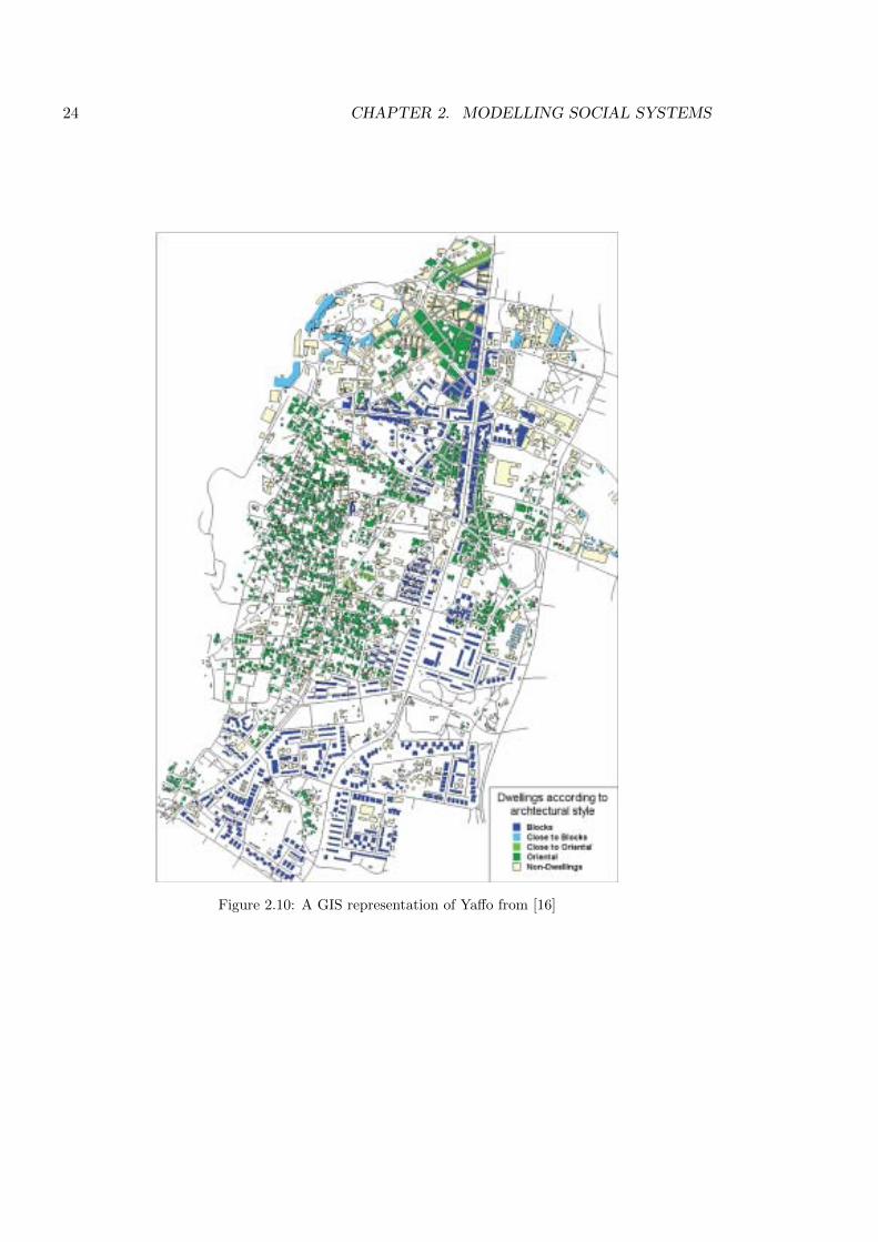
24 CHAPTER 2. MODELLING SOCIAL SYSTEMS
Why Is the Yaffo Model so Insensitive to Parameters?
The reason for the Yaffo model’s robustness was the ‘‘try the better’’(TRB) algorithm of residential choice we formulated. An agent who usesTRB orders opportunities by their utilities prior to making a choice
Figure 1Yaffo Model: (a) Definition of the Neighborhood Relationships
and (b) Map of Buildings’ Architectural Styles
Source: Benenson et al. (2002).
Table 1Correspondence Between the Yaffo Model and Reality, 1995
Measure of Correspondence Yaffo Model
Overall percentage of Arab agents in the area 32.2 34.8
Moran index I for Arab agents 0.65 0.66
Percentage of Jewish agents in houses of oriental style 28.1 15.0
Percentage of Arab agents in houses of block style 18.5 8.0
Benenson et al. / Spatially Explicit Modeling 473
at University of York on March 22, 2010 http://smr.sagepub.comDownloaded from
Figure 2.10: A GIS representation of Ya↵o from [16]
2.6. GEOGRAPHIC INFORMATION SYSTEMS 25
Why Is the Yaffo Model so Insensitive to Parameters?
The reason for the Yaffo model’s robustness was the ‘‘try the better’’(TRB) algorithm of residential choice we formulated. An agent who usesTRB orders opportunities by their utilities prior to making a choice
Figure 1Yaffo Model: (a) Definition of the Neighborhood Relationships
and (b) Map of Buildings’ Architectural Styles
Source: Benenson et al. (2002).
Table 1Correspondence Between the Yaffo Model and Reality, 1995
Measure of Correspondence Yaffo Model
Overall percentage of Arab agents in the area 32.2 34.8
Moran index I for Arab agents 0.65 0.66
Percentage of Jewish agents in houses of oriental style 28.1 15.0
Percentage of Arab agents in houses of block style 18.5 8.0
Benenson et al. / Spatially Explicit Modeling 473
at University of York on March 22, 2010 http://smr.sagepub.comDownloaded from
Figure 2.11: An example neighbourhood from [16]
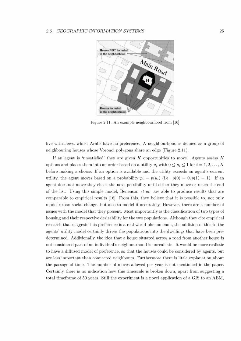
live with Jews, whilst Arabs have no preference. A neighbourhood is defined as a group of
neighbouring houses whose Voronoi polygons share an edge (Figure 2.11).
If an agent is ‘unsatisfied’ they are given K opportunities to move. Agents assess K
options and places them into an order based on a utility ui with 0 ui 1 for i = 1, 2, . . . ,K
before making a choice. If an option is available and the utility exceeds an agent’s current
utility, the agent moves based on a probability pi = p(ui) (i.e. p(0) = 0, p(1) = 1). If an
agent does not move they check the next possibility until either they move or reach the end
of the list. Using this simple model, Benenson et al. are able to produce results that are
comparable to empirical results [16]. From this, they believe that it is possible to, not only
model urban social change, but also to model it accurately. However, there are a number of
issues with the model that they present. Most importantly is the classification of two types of
housing and their respective desirability for the two populations. Although they cite empirical
research that suggests this preference is a real world phenomenon, the addition of this to the
agents’ utility model certainly drives the populations into the dwellings that have been pre-
determined. Additionally, the idea that a house situated across a road from another house is
not considered part of an individual’s neighbourhood is unrealistic. It would be more realistic
to have a di↵used model of preference, so that the houses could be considered by agents, but
are less important than connected neighbours. Furthermore there is little explanation about
the passage of time. The number of moves allowed per year is not mentioned in the paper.
Certainly there is no indication how this timescale is broken down, apart from suggesting a
total timeframe of 50 years. Still the experiment is a novel application of a GIS to an ABM,
26 CHAPTER 2. MODELLING SOCIAL SYSTEMS
and should be an important tool in future research.
More recently, ideas of Participatory GISs have been advocated. Participatory GIS looks
to utilise the knowledge of local communities to enhance the applications of GISs. It is hoped
that by combining GISs and Participatory Learning and Action PGISs will increase the use-
fulness of GISs [26]. By inviting this input it is hoped the previously static nature of GISs can
become more dynamic and responsive to the needs of users. The practice integrates several
tools and methods whilst often relying on the combination of expert skills with socially dif-
ferentiated local knowledge [26]. It promotes interactive participation of stakeholders in gen-
erating and managing spatial information and it uses information about specific landscapes
to facilitate broadly-based decision making processes that support e↵ective communication
and community advocacy [26]. However the approach is limited to technologically confident
participants, meaning some important stakeholders could be missed.
2.7 Summary
One of the problems of dealing with complex systems is that complexity is not boolean.
Rather, complexity can be considered a scale from simple complex systems, such as reacting
particles, to highly complex systems, such as social systems. Additionally the complexity
can be in both the environment and the components within the environment. The problem
is probably best described by Herb Simon’s ‘situated ant’ [83]. An ant following a random
walk on a beach produces a complex path. An observer watching might be amazed at this
complexity created by the ant. However, Simon suggests, the complexity of the environment
is creating the complex path rather than the ant. The analogy suggests complexity of the
environment is as important as the complexity of the individual.
From the previous sections, it would appear that complex systems can be considered (at
least) an individual situated within an interacting environment. By creating a matrix based
on the complexities of both the environment and the individuals one should be able to classify
the system being studied accordingly. Taking the environment as the horizontal axis, it is
clear there are a number of ways to represent the environment. Aspatial environments are
probably the simplest since their is no spatial representation, the environment is considered
just the mixture of individuals. Network space is a graphical representation of connections
(often called vertices) between individuals (nodes). Distance is considered in terms of the
number of nodes between two individual nodes, rather than Euclidean distance along the
links. Structured space has a notion of distance between nodes but it is not a metric as
it does not satisfy the triangle inequality (i.e., for the distance between two nodes, A and
C, is not necessarily less than or equal to the distance between A and B plus B and C).
2.7. SUMMARY 27
Figure 2.12: The Social Simulation Matrix. D.E = Di↵erential Equation. As space and agencycomplexity increase, di↵erent modelling techniques are needed to capture the increased complexity.The matrix is an attempt to map techniques in modelling social systems to the complexity of the objectbeing modelled. The matrix highlights the breath of modelling covered by Agent Based Models.
28 CHAPTER 2. MODELLING SOCIAL SYSTEMS
Moving away from these abstract notions we come to simple homogeneous space. Here
the environment is a uniform collection of Euclidian space incorporating ideas of distance
and location. Introducing variation in the space takes us to heterogeneous space. Now
di↵erent spatial locations can have di↵erent attributes. Increasing the heterogeneity of the
environment eventually brings us to geographical space which can be considered an almost
one to one mapping with a ‘real-world’ environment.
Individuals within the environments can be scaled according to agency. By this we mean
an ability to act independently and make choices based on available information. The sim-
plest form of agency is a population level, statelessness form. Individual components are
indistinguishable and, therefore, treated as a continuum rather than as single components.
Identifying individual components allows us to introduce ideas of agency properly, the sim-
plest form of which is passive components. As the name suggests these components are
unable to respond to any changes in their environment and continue with their set goal
irrespective of external influence. More complex reactive components are able to react to
environmental changes to achieve goals. This reaction is based on a hierarchical set of be-
havioural rules. Hybrid components introduce a subsystem responsible for abstract planning
and decision making. Adaptive components are similar to hybrids but have an important
addition, namely they are able to learn from their environment. Whilst reactive and hybrid
components have a knowledge about their environment, adaptive components have additional
knowledge about their own structure and evolutionary capacity. This knowledge and learning
ability allows components to adapt their behaviours to reach their goal. Finally cognitive
components are able to create a symbolic internalised model of their environment. From this
model they are able to reason and plan strategies to achieve their goal.
By plotting these two aspects of a system we can produce the social simulation matrix in
Figure 2.12. The matrix can be used to guide the process of selecting a modelling tool for the
task at hand. As complex systems are multi-faceted, the toolset needed for analysis can be
compared to the Swiss army knife. The very nature of a complex system requires many tools
to process the huge amount of information. With so many tools available to model social
systems it is useful to map the available techniques onto the social simulation matrix. The
development of these (and other) techniques using computational modelling and simulation,
has led to the birth of Computational Social Science [29]. One of the most well used models
in the field is Schelling’s ‘Dynamic Models of Segregation’, which is now introduced in detail.
Chapter 3
Schelling’s models of Segregation
Schelling’s models of segregation have been the focus of a number of studies using a variety of
di↵erent techniques. In his ground breaking paper [74], Schelling used ABMs to explore ideas
of segregation in heterogeneous populations. The models he developed used simplified ideas
of social interaction. As has been mentioned, this has been described as the first ABM [30].
It has also been called the first simulation of an artificial society [73]. Although described
as ‘elegant’ [28], Schelling’s models are at times confused (for example, Axelrod talks of
Schelling’s Bounded Neighbourhood Model but describes the Spatial Proximity Model [10])
and closer analysis reveals intricacies (such as the movement of the agents) that have been
overlooked. Schelling actually describes two distinct models, a Spatial Proximity Model [74,
p149] and a Bounded Neighbourhood Model [74, p167]. Finally he combines aspects of the
two into a Tipping Model [74, p181]. His models are now described in detail.
3.1 Spatial Proximity Model
The Spatial Proximity Model explores the aggregate/global e↵ects of two groups of characters
making decisions based on a local neighbourhood N for each character. Schelling created a
one dimensional environment with two types of characters, equal in number and randomly
arranged along the environment. The environment was Schelling’s typewriter which defined
the limits of 70 characters per line. Each character has a location, a thresholded ‘happiness’
about the makeup of their own neighbourhood N and a movement rule. An example of the
system can be seen in Figure 3.1. For characters situated a distance of at least n from the
boundary, Schelling chooses the neighbourhood N to contain 2n characters, n on the left and
n on the right. For characters closer to the boundary, say m < n units, he considers a reduced
29
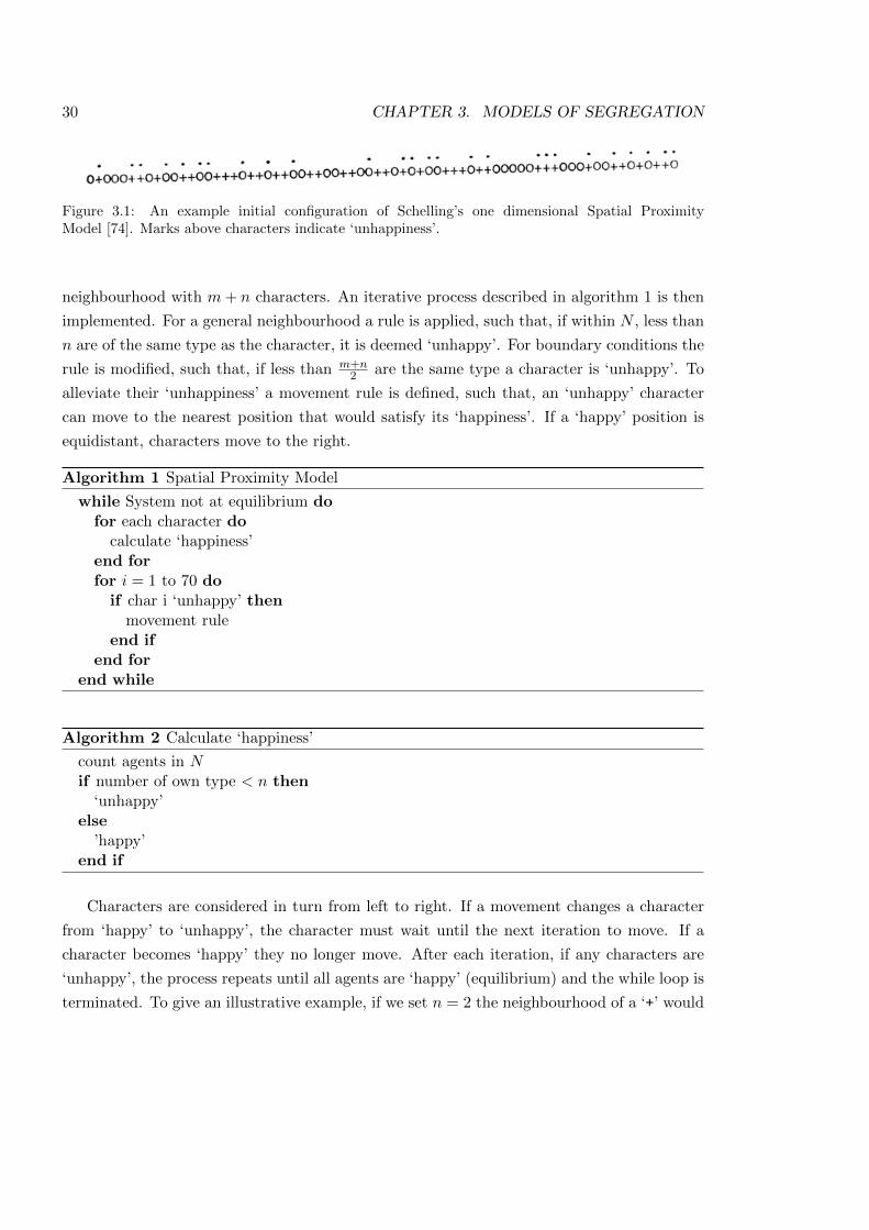
30 CHAPTER 3. MODELS OF SEGREGATION
Figure 3.1: An example initial configuration of Schelling’s one dimensional Spatial ProximityModel [74]. Marks above characters indicate ‘unhappiness’.
neighbourhood with m+ n characters. An iterative process described in algorithm 1 is then
implemented. For a general neighbourhood a rule is applied, such that, if within N , less than
n are of the same type as the character, it is deemed ‘unhappy’. For boundary conditions the
rule is modified, such that, if less than m+n2 are the same type a character is ‘unhappy’. To
alleviate their ‘unhappiness’ a movement rule is defined, such that, an ‘unhappy’ character
can move to the nearest position that would satisfy its ‘happiness’. If a ‘happy’ position is
equidistant, characters move to the right.
Algorithm 1 Spatial Proximity Model
while System not at equilibrium dofor each character do
calculate ‘happiness’end forfor i = 1 to 70 do
if char i ‘unhappy’ thenmovement rule
end ifend for
end while
Algorithm 2 Calculate ‘happiness’
count agents in Nif number of own type < n then‘unhappy’
else’happy’
end if
Characters are considered in turn from left to right. If a movement changes a character
from ‘happy’ to ‘unhappy’, the character must wait until the next iteration to move. If a
character becomes ‘happy’ they no longer move. After each iteration, if any characters are
‘unhappy’, the process repeats until all agents are ‘happy’ (equilibrium) and the while loop is
terminated. To give an illustrative example, if we set n = 2 the neighbourhood of a ‘+’ would
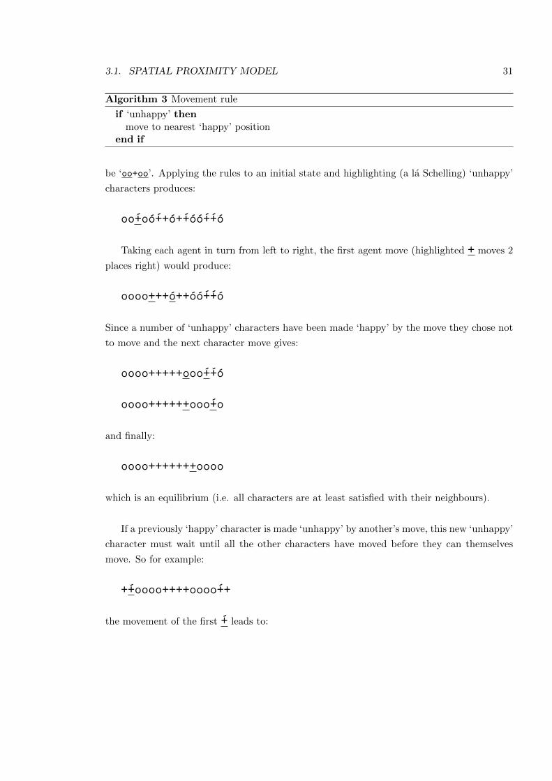
3.1. SPATIAL PROXIMITY MODEL 31
Algorithm 3 Movement rule
if ‘unhappy’ thenmove to nearest ‘happy’ position
end if
be ‘oo+oo’. Applying the rules to an initial state and highlighting (a la Schelling) ‘unhappy’
characters produces:
oo
´
+oo
´
++o+
´
+oo
´
+
´
+o
Taking each agent in turn from left to right, the first agent move (highlighted + moves 2
places right) would produce:
oooo+++o++oo
´
+
´
+o
Since a number of ‘unhappy’ characters have been made ‘happy’ by the move they chose not
to move and the next character move gives:
oooo+++++ooo
´
+
´
+o
oooo++++++ooo
´
+o
and finally:
oooo+++++++oooo
which is an equilibrium (i.e. all characters are at least satisfied with their neighbours).
If a previously ‘happy’ character is made ‘unhappy’ by another’s move, this new ‘unhappy’
character must wait until all the other characters have moved before they can themselves
move. So for example:
+
´
+oooo++++oooo
´
++
the movement of the first ´+ leads to:

32 CHAPTER 3. MODELS OF SEGREGATION
+oooo+++++oooo
´
++
which creates a newly ‘unhappy’ character (the leftmost +). This character must wait for
the iteration to complete before itself moving.
Schelling concludes that, with all things being equal, di↵erent random sequences of 70
characters with n = 4 “... yield[s] from about five groupings with an average of 14 members
to about seven or eight groupings with an average of 9 or 10, six being the modal number of
groups and 12 the modal size.”
To highlight this finding two di↵erent initial configurations with the same ruleset are ex-
plored below. If a character is equidistant from a ‘happy’ position, it will move to the right.
The first configuration achieves equilibrium after one iteration:
o+++++oo++ooo++oo+++oooo++++ooo+++++oooooo+++oooo++++oooooo++o++ooo+++
+++++++oooooooooooo++++++++++++++ooooooooooooo+++++++oooooooooo+++++++
as does the second:
++o++o++oo+++ooo++++ooo++oooo+++ooooo++++oo++++oo+oo+ooo++++ooo++ooo+o
+++++++++ooooooo++++++oooooooooooo++++++++++++oooooooooo++++++++oooooo
A third configuration has two runs to explore the e↵ect of the movement rule. The first
is from Schelling’s movement rule:
oo+++ooo+++oo+++oo+++oooo+++oooo+++ooo++ooo+++ooo+o+o+++ooo++++oooo+++
+ooooooo+++++++++++ooooooooo+++o+++o++oooooooooo++++++++++++++ooooooo+
ooooooo++++++++++++oooooooooo++++++++ooooooooooo+++++++++++++++ooooooo
and the second from modifying a movement rule to consider the characters in a random order
(rather than the sequential left to right order):
oo+++ooo+++oo+++oo+++oooo+++oooo+++ooo++ooo+++ooo+o+o+++ooo++++oooo+++
ooooooo++++++++++++++ooooooooooo++++++oooooooooo++++++++++++++ooooooo+
ooooooo++++++++++++++ooooooooooo++++++oooooooooo+++++++++++++++ooooooo
As these results show, the movement rule of left to right or random does not produce
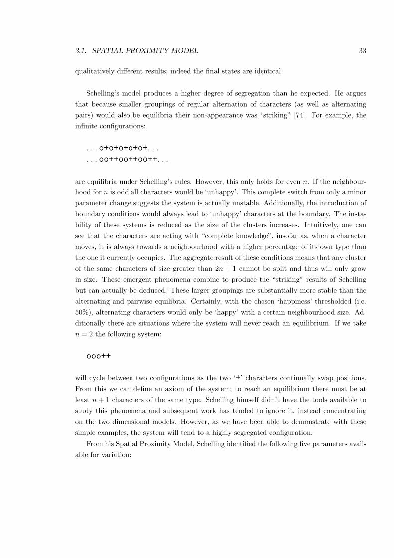
3.1. SPATIAL PROXIMITY MODEL 33
qualitatively di↵erent results; indeed the final states are identical.
Schelling’s model produces a higher degree of segregation than he expected. He argues
that because smaller groupings of regular alternation of characters (as well as alternating
pairs) would also be equilibria their non-appearance was “striking” [74]. For example, the
infinite configurations:
. . . o+o+o+o+o+. . .
. . . oo++oo++oo++. . .
are equilibria under Schelling’s rules. However, this only holds for even n. If the neighbour-
hood for n is odd all characters would be ‘unhappy’. This complete switch from only a minor
parameter change suggests the system is actually unstable. Additionally, the introduction of
boundary conditions would always lead to ‘unhappy’ characters at the boundary. The insta-
bility of these systems is reduced as the size of the clusters increases. Intuitively, one can
see that the characters are acting with “complete knowledge”, insofar as, when a character
moves, it is always towards a neighbourhood with a higher percentage of its own type than
the one it currently occupies. The aggregate result of these conditions means that any cluster
of the same characters of size greater than 2n + 1 cannot be split and thus will only grow
in size. These emergent phenomena combine to produce the “striking” results of Schelling
but can actually be deduced. These larger groupings are substantially more stable than the
alternating and pairwise equilibria. Certainly, with the chosen ‘happiness’ thresholded (i.e.
50%), alternating characters would only be ‘happy’ with a certain neighbourhood size. Ad-
ditionally there are situations where the system will never reach an equilibrium. If we take
n = 2 the following system:
ooo++
will cycle between two configurations as the two ‘+’ characters continually swap positions.
From this we can define an axiom of the system; to reach an equilibrium there must be at
least n + 1 characters of the same type. Schelling himself didn’t have the tools available to
study this phenomena and subsequent work has tended to ignore it, instead concentrating
on the two dimensional models. However, as we have been able to demonstrate with these
simple examples, the system will tend to a highly segregated configuration.
From his Spatial Proximity Model, Schelling identified the following five parameters avail-
able for variation:
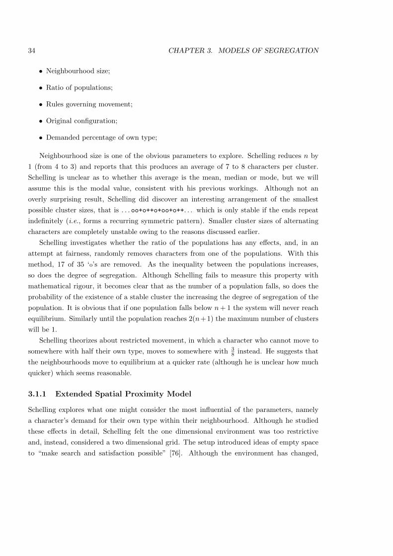
34 CHAPTER 3. MODELS OF SEGREGATION
• Neighbourhood size;
• Ratio of populations;
• Rules governing movement;
• Original configuration;
• Demanded percentage of own type;
Neighbourhood size is one of the obvious parameters to explore. Schelling reduces n by
1 (from 4 to 3) and reports that this produces an average of 7 to 8 characters per cluster.
Schelling is unclear as to whether this average is the mean, median or mode, but we will
assume this is the modal value, consistent with his previous workings. Although not an
overly surprising result, Schelling did discover an interesting arrangement of the smallest
possible cluster sizes, that is . . . oo+o++o+oo+o++. . . which is only stable if the ends repeat
indefinitely (i.e., forms a recurring symmetric pattern). Smaller cluster sizes of alternating
characters are completely unstable owing to the reasons discussed earlier.
Schelling investigates whether the ratio of the populations has any e↵ects, and, in an
attempt at fairness, randomly removes characters from one of the populations. With this
method, 17 of 35 ‘o’s are removed. As the inequality between the populations increases,
so does the degree of segregation. Although Schelling fails to measure this property with
mathematical rigour, it becomes clear that as the number of a population falls, so does the
probability of the existence of a stable cluster the increasing the degree of segregation of the
population. It is obvious that if one population falls below n+ 1 the system will never reach
equilibrium. Similarly until the population reaches 2(n+1) the maximum number of clusters
will be 1.
Schelling theorizes about restricted movement, in which a character who cannot move to
somewhere with half their own type, moves to somewhere with 38 instead. He suggests that
the neighbourhoods move to equilibrium at a quicker rate (although he is unclear how much
quicker) which seems reasonable.
3.1.1 Extended Spatial Proximity Model
Schelling explores what one might consider the most influential of the parameters, namely
a character’s demand for their own type within their neighbourhood. Although he studied
these e↵ects in detail, Schelling felt the one dimensional environment was too restrictive
and, instead, considered a two dimensional grid. The setup introduced ideas of empty space
to “make search and satisfaction possible” [76]. Although the environment has changed,
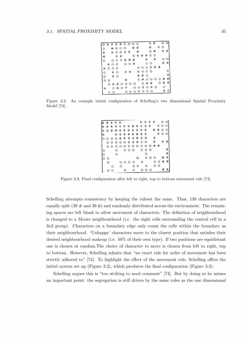
3.1. SPATIAL PROXIMITY MODEL 35
Figure 3.2: An example initial configuration of Schelling’s two dimensional Spatial ProximityModel [74].
Figure 3.3: Final configuration after left to right, top to bottom movement rule [74].
Schelling attempts consistency by keeping the ruleset the same. Thus, 138 characters are
equally split (39 # and 39 o) and randomly distributed across the environment. The remain-
ing spaces are left blank to allow movement of characters. The definition of neighbourhood
is changed to a Moore neighbourhood (i.e. the eight cells surrounding the central cell in a
3x3 group). Characters on a boundary edge only count the cells within the boundary as
their neighbourhood. ‘Unhappy’ characters move to the closest position that satisfies their
desired neighbourhood makeup (i.e. 50% of their own type). If two positions are equidistant
one is chosen at random.The choice of character to move is chosen from left to right, top
to bottom. However, Schelling admits that “no exact rule for order of movement has been
strictly adhered to” [74]. To highlight the e↵ect of the movement rule, Schelling o↵ers the
initial system set up (Figure 3.2), which produces the final configuration (Figure 3.3).
Schelling argues this is “too striking to need comment” [74]. But by doing so he misses
an important point: the segregation is still driven by the same rules as the one dimensional
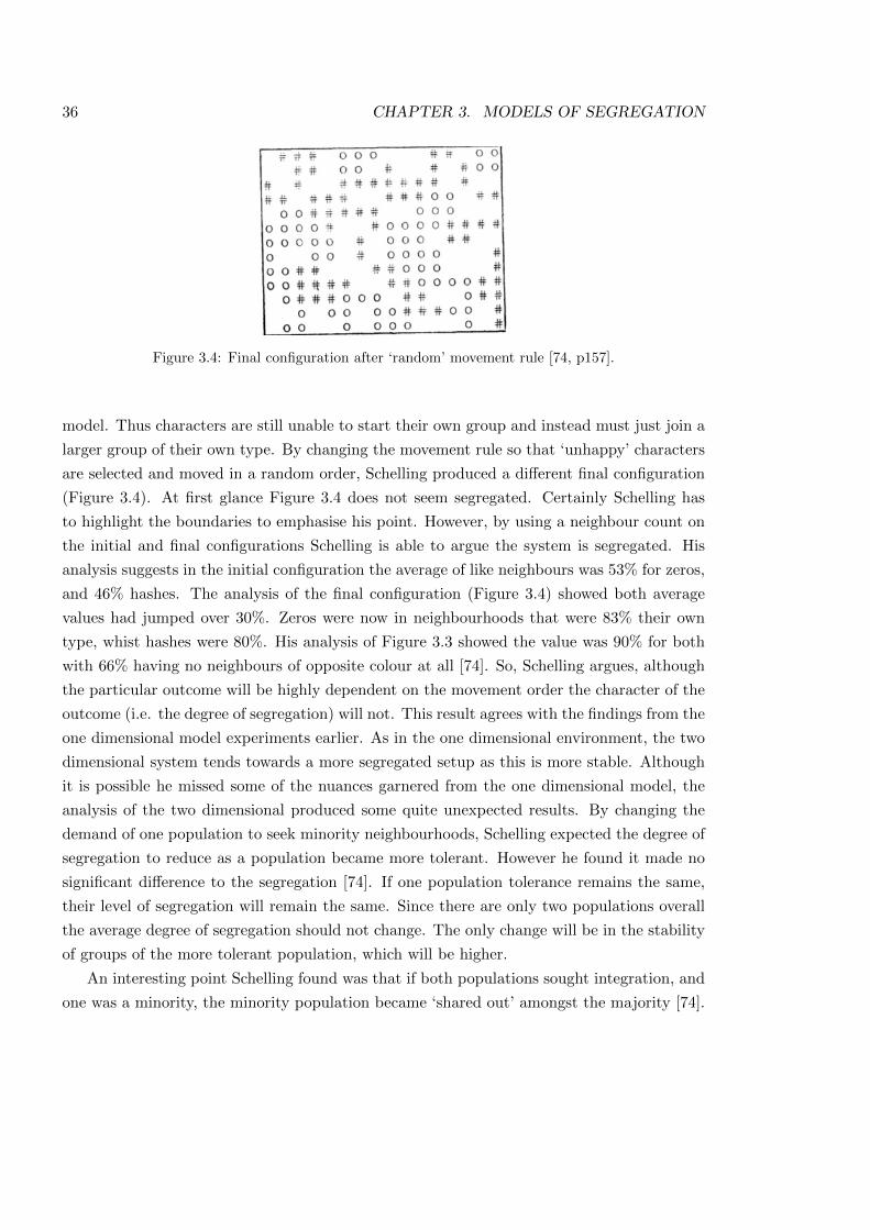
36 CHAPTER 3. MODELS OF SEGREGATION
Figure 3.4: Final configuration after ‘random’ movement rule [74, p157].
model. Thus characters are still unable to start their own group and instead must just join a
larger group of their own type. By changing the movement rule so that ‘unhappy’ characters
are selected and moved in a random order, Schelling produced a di↵erent final configuration
(Figure 3.4). At first glance Figure 3.4 does not seem segregated. Certainly Schelling has
to highlight the boundaries to emphasise his point. However, by using a neighbour count on
the initial and final configurations Schelling is able to argue the system is segregated. His
analysis suggests in the initial configuration the average of like neighbours was 53% for zeros,
and 46% hashes. The analysis of the final configuration (Figure 3.4) showed both average
values had jumped over 30%. Zeros were now in neighbourhoods that were 83% their own
type, whist hashes were 80%. His analysis of Figure 3.3 showed the value was 90% for both
with 66% having no neighbours of opposite colour at all [74]. So, Schelling argues, although
the particular outcome will be highly dependent on the movement order the character of the
outcome (i.e. the degree of segregation) will not. This result agrees with the findings from the
one dimensional model experiments earlier. As in the one dimensional environment, the two
dimensional system tends towards a more segregated setup as this is more stable. Although
it is possible he missed some of the nuances garnered from the one dimensional model, the
analysis of the two dimensional produced some quite unexpected results. By changing the
demand of one population to seek minority neighbourhoods, Schelling expected the degree of
segregation to reduce as a population became more tolerant. However he found it made no
significant di↵erence to the segregation [74]. If one population tolerance remains the same,
their level of segregation will remain the same. Since there are only two populations overall
the average degree of segregation should not change. The only change will be in the stability
of groups of the more tolerant population, which will be higher.
An interesting point Schelling found was that if both populations sought integration, and
one was a minority, the minority population became ‘shared out’ amongst the majority [74].
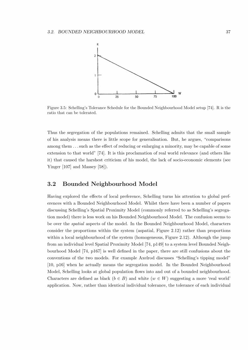
3.2. BOUNDED NEIGHBOURHOOD MODEL 37
Figure 3.5: Schelling’s Tolerance Schedule for the Bounded Neighbourhood Model setup [74]. R is theratio that can be tolerated.
Thus the segregation of the populations remained. Schelling admits that the small sample
of his analysis means there is little scope for generalisation. But, he argues, “comparisons
among them . . . such as the e↵ect of reducing or enlarging a minority, may be capable of some
extension to that world” [74]. It is this proclamation of real world relevance (and others like
it) that caused the harshest criticism of his model, the lack of socio-economic elements (see
Yinger [107] and Massey [58]).
3.2 Bounded Neighbourhood Model
Having explored the e↵ects of local preference, Schelling turns his attention to global pref-
erences with a Bounded Neighbourhood Model. Whilst there have been a number of papers
discussing Schelling’s Spatial Proximity Model (commonly referred to as Schelling’s segrega-
tion model) there is less work on his Bounded Neighbourhood Model. The confusion seems to
be over the spatial aspects of the model. In the Bounded Neighbourhood Model, characters
consider the proportions within the system (aspatial, Figure 2.12) rather than proportions
within a local neighbourhood of the system (homogeneous, Figure 2.12). Although the jump
from an individual level Spatial Proximity Model [74, p149] to a system level Bounded Neigh-
bourhood Model [74, p167] is well defined in the paper, there are still confusions about the
conventions of the two models. For example Axelrod discusses “Schelling’s tipping model”
[10, p16] when he actually means the segregation model. In the Bounded Neighbourhood
Model, Schelling looks at global population flows into and out of a bounded neighbourhood.
Characters are defined as black (b 2 B) and white (w 2 W ) suggesting a more ‘real world’
application. Now, rather than identical individual tolerance, the tolerance of each individual

38 CHAPTER 3. MODELS OF SEGREGATION
is defined by a straight line cumulative distribution schedule plotted against R, the ratio that
a character is willing to accept in the neighbourhood, with a maximum of R = 2 (i.e., a ratio
of 2:1) (Figure 3.5).
Thus, according to Schelling,
“for each number of whites along the horizontal axis the number of blacks whose
presence they will tolerate is equal to their own number times the corresponding
ratio [on Figure 3.5].”
The schedule is applied at a population level. That is, for a population of 100W ; 25W can
tolerate 37.5B (25⇥ 1.5), 50W can tolerate 50B, 75W can tolerate 37.5B (75⇥ 0.5) and the
most tolerant W is ‘happy’ with two Bs for each W . So long as the system configuration
lies below the curve, the population is ‘happy’. If the system lies above the line (i.e. W =
100, R = 1), there will be ‘unhappy’ members of the population. The tolerance schedule is
applied to both populations B and W irrespective of whether they are inside or outside of
the bounded neighbourhood. Thus, those outside the system will enter based on the current
make up of the system population.
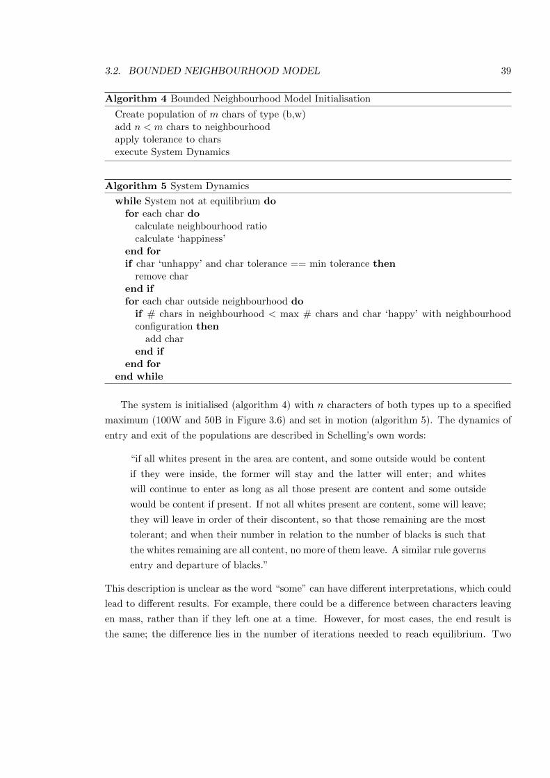
3.2. BOUNDED NEIGHBOURHOOD MODEL 39
Algorithm 4 Bounded Neighbourhood Model Initialisation
Create population of m chars of type (b,w)add n < m chars to neighbourhoodapply tolerance to charsexecute System Dynamics
Algorithm 5 System Dynamics
while System not at equilibrium dofor each char do
calculate neighbourhood ratiocalculate ‘happiness’
end forif char ‘unhappy’ and char tolerance == min tolerance then
remove charend iffor each char outside neighbourhood do
if # chars in neighbourhood < max # chars and char ‘happy’ with neighbourhoodconfiguration thenadd char
end ifend for
end while
The system is initialised (algorithm 4) with n characters of both types up to a specified
maximum (100W and 50B in Figure 3.6) and set in motion (algorithm 5). The dynamics of
entry and exit of the populations are described in Schelling’s own words:
“if all whites present in the area are content, and some outside would be content
if they were inside, the former will stay and the latter will enter; and whites
will continue to enter as long as all those present are content and some outside
would be content if present. If not all whites present are content, some will leave;
they will leave in order of their discontent, so that those remaining are the most
tolerant; and when their number in relation to the number of blacks is such that
the whites remaining are all content, no more of them leave. A similar rule governs
entry and departure of blacks.”
This description is unclear as the word “some” can have di↵erent interpretations, which could
lead to di↵erent results. For example, there could be a di↵erence between characters leaving
en mass, rather than if they left one at a time. However, for most cases, the end result is
the same; the di↵erence lies in the number of iterations needed to reach equilibrium. Two
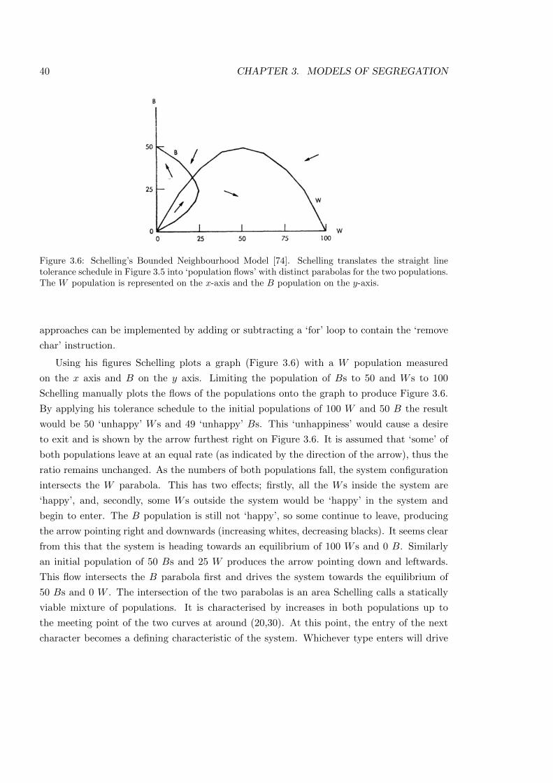
40 CHAPTER 3. MODELS OF SEGREGATION
Figure 3.6: Schelling’s Bounded Neighbourhood Model [74]. Schelling translates the straight linetolerance schedule in Figure 3.5 into ‘population flows’ with distinct parabolas for the two populations.The W population is represented on the x-axis and the B population on the y-axis.
approaches can be implemented by adding or subtracting a ‘for’ loop to contain the ‘remove
char’ instruction.
Using his figures Schelling plots a graph (Figure 3.6) with a W population measured
on the x axis and B on the y axis. Limiting the population of Bs to 50 and W s to 100
Schelling manually plots the flows of the populations onto the graph to produce Figure 3.6.
By applying his tolerance schedule to the initial populations of 100 W and 50 B the result
would be 50 ‘unhappy’ W s and 49 ‘unhappy’ Bs. This ‘unhappiness’ would cause a desire
to exit and is shown by the arrow furthest right on Figure 3.6. It is assumed that ‘some’ of
both populations leave at an equal rate (as indicated by the direction of the arrow), thus the
ratio remains unchanged. As the numbers of both populations fall, the system configuration
intersects the W parabola. This has two e↵ects; firstly, all the W s inside the system are
‘happy’, and, secondly, some W s outside the system would be ‘happy’ in the system and
begin to enter. The B population is still not ‘happy’, so some continue to leave, producing
the arrow pointing right and downwards (increasing whites, decreasing blacks). It seems clear
from this that the system is heading towards an equilibrium of 100 W s and 0 B. Similarly
an initial population of 50 Bs and 25 W produces the arrow pointing down and leftwards.
This flow intersects the B parabola first and drives the system towards the equilibrium of
50 Bs and 0 W . The intersection of the two parabolas is an area Schelling calls a statically
viable mixture of populations. It is characterised by increases in both populations up to
the meeting point of the two curves at around (20,30). At this point, the entry of the next
character becomes a defining characteristic of the system. Whichever type enters will drive
3.2. BOUNDED NEIGHBOURHOOD MODEL 41
Figure 3.7: Schelling’s Bounded Neighbourhood model setup with equal populations and 5:1 toler-ance [74].
the system to their equilibrium. Thus, the point bears the hallmarks of an unstable fixed
point, whilst the parabolas can be considered null clines. However, the language of dynamical
systems was in its infancy at this time, and ‘unstable fixed point’ and ‘null clines’ were terms
Schelling may have been unaware of. The figures certainly have a similarity to the phase
portraits of non-linear systems. The arrows suggest the flow of the population and Schelling
talks of equilibrium points at (0,50) and (100,0).
Schelling now defines two parameters to explore, namely population size and the toler-
ance schedule. By levelling the population sizes and increasing the tolerance schedule to a
maximum of 5:1 he produces Figure 3.7. An analysis of the this configuration displays what
Schelling calls a “mixed equilibrium” [74] at (80,80). Schelling suggests the mixed equilibrium
is stable so long as “slightly over 40%” of both colours are present and the entry of one is
“not much more rapid” than the other. The arrows would suggest the point corresponds to
a stable fixed point.
In another experiment, Schelling explores the e↵ects of limiting the ratios by restricting
the entry of a population. So that, for example, if the ratio of white to black is exceeded
no more whites may enter (although blacks are free to leave). The result (with symmetric
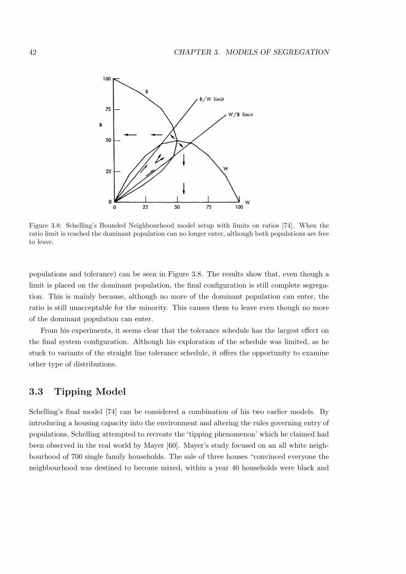
42 CHAPTER 3. MODELS OF SEGREGATION
Figure 3.8: Schelling’s Bounded Neighbourhood model setup with limits on ratios [74]. When theratio limit is reached the dominant population can no longer enter, although both populations are freeto leave.
populations and tolerance) can be seen in Figure 3.8. The results show that, even though a
limit is placed on the dominant population, the final configuration is still complete segrega-
tion. This is mainly because, although no more of the dominant population can enter, the
ratio is still unacceptable for the minority. This causes them to leave even though no more
of the dominant population can enter.
From his experiments, it seems clear that the tolerance schedule has the largest e↵ect on
the final system configuration. Although his exploration of the schedule was limited, as he
stuck to variants of the straight line tolerance schedule, it o↵ers the opportunity to examine
other type of distributions.
3.3 Tipping Model
Schelling’s final model [74] can be considered a combination of his two earlier models. By
introducing a housing capacity into the environment and altering the rules governing entry of
populations, Schelling attempted to recreate the ‘tipping phenomenon’ which he claimed had
been observed in the real world by Mayer [60]. Mayer’s study focused on an all white neigh-
bourhood of 700 single family households. The sale of three houses “convinced everyone the
neighbourhood was destined to become mixed, within a year 40 households were black and
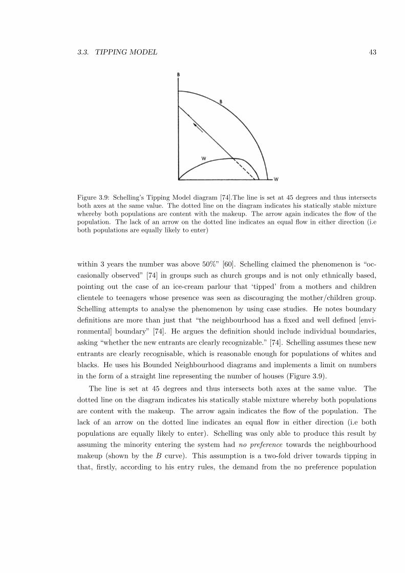
3.3. TIPPING MODEL 43
Figure 3.9: Schelling’s Tipping Model diagram [74].The line is set at 45 degrees and thus intersectsboth axes at the same value. The dotted line on the diagram indicates his statically stable mixturewhereby both populations are content with the makeup. The arrow again indicates the flow of thepopulation. The lack of an arrow on the dotted line indicates an equal flow in either direction (i.eboth populations are equally likely to enter)
within 3 years the number was above 50%” [60]. Schelling claimed the phenomenon is “oc-
casionally observed” [74] in groups such as church groups and is not only ethnically based,
pointing out the case of an ice-cream parlour that ‘tipped’ from a mothers and children
clientele to teenagers whose presence was seen as discouraging the mother/children group.
Schelling attempts to analyse the phenomenon by using case studies. He notes boundary
definitions are more than just that “the neighbourhood has a fixed and well defined [envi-
ronmental] boundary” [74]. He argues the definition should include individual boundaries,
asking “whether the new entrants are clearly recognizable.” [74]. Schelling assumes these new
entrants are clearly recognisable, which is reasonable enough for populations of whites and
blacks. He uses his Bounded Neighbourhood diagrams and implements a limit on numbers
in the form of a straight line representing the number of houses (Figure 3.9).
The line is set at 45 degrees and thus intersects both axes at the same value. The
dotted line on the diagram indicates his statically stable mixture whereby both populations
are content with the makeup. The arrow again indicates the flow of the population. The
lack of an arrow on the dotted line indicates an equal flow in either direction (i.e both
populations are equally likely to enter). Schelling was only able to produce this result by
assuming the minority entering the system had no preference towards the neighbourhood
makeup (shown by the B curve). This assumption is a two-fold driver towards tipping in
that, firstly, according to his entry rules, the demand from the no preference population
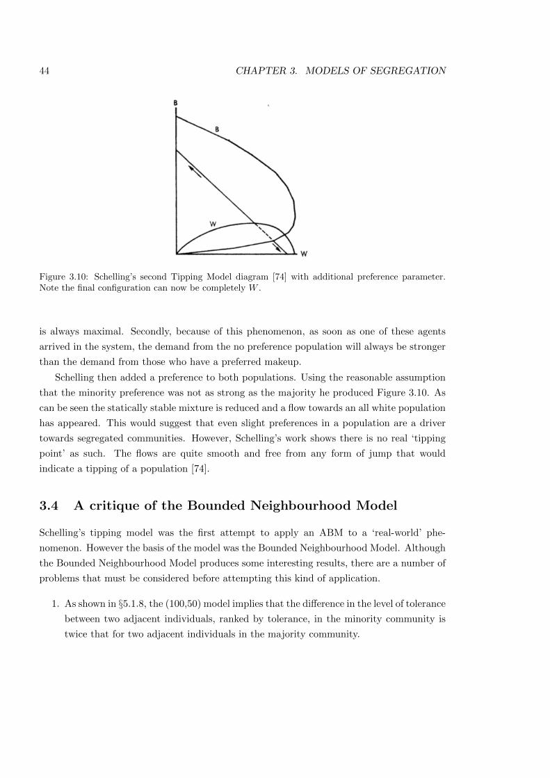
44 CHAPTER 3. MODELS OF SEGREGATION
Figure 3.10: Schelling’s second Tipping Model diagram [74] with additional preference parameter.Note the final configuration can now be completely W .
is always maximal. Secondly, because of this phenomenon, as soon as one of these agents
arrived in the system, the demand from the no preference population will always be stronger
than the demand from those who have a preferred makeup.
Schelling then added a preference to both populations. Using the reasonable assumption
that the minority preference was not as strong as the majority he produced Figure 3.10. As
can be seen the statically stable mixture is reduced and a flow towards an all white population
has appeared. This would suggest that even slight preferences in a population are a driver
towards segregated communities. However, Schelling’s work shows there is no real ‘tipping
point’ as such. The flows are quite smooth and free from any form of jump that would
indicate a tipping of a population [74].
3.4 A critique of the Bounded Neighbourhood Model
Schelling’s tipping model was the first attempt to apply an ABM to a ‘real-world’ phe-
nomenon. However the basis of the model was the Bounded Neighbourhood Model. Although
the Bounded Neighbourhood Model produces some interesting results, there are a number of
problems that must be considered before attempting this kind of application.
1. As shown in §5.1.8, the (100,50) model implies that the di↵erence in the level of tolerance
between two adjacent individuals, ranked by tolerance, in the minority community is
twice that for two adjacent individuals in the majority community.
3.5. CONCLUSIONS 45
2. Not surprisingly a su�ciently high tolerance ⌧ will ensure the existence of subsets of
the two communities that can coexist ‘stably’, in the sense that no-one wishes to leave.
3. The Bounded Neighbourhood Model can be seen as a deterministic model certainly once
the movement rule has been clearly defined it is quite simple to work out the results.
Whilst this allows stringent testing of the simulation accuracy against the model it is
so simplistic that it cannot be said to have any bearing on reality.
4. Although agents distinguish between type, there is no di↵erence within type (i.e., all
whites are the same and all blacks are the same).
3.5 Conclusions
The popularity of Schelling’s ideas led to criticisms most notably, Yinger [107], who argued
that there was no consideration of a number of factors such as economics and social mobility.
Similarly, Massey [58], argued that not accounting for environmental/spacial factors and using
a homogenous environment meant the model was too simplistic to have any relation to reality.
These were the main criticisms, suggesting that simplistic models cannot capture enough
information about what really drives segregation. Simple notions of preference, although they
probably exist, are superseded by the more important factors of economics and social mobility.
Today this could be a fair criticism since the input of experts in the field is an important
part of the modelling process. But what Schelling was suggesting with his models is a far
cry from the criticisms of Yinger and Massey. Schelling demonstrated that a simple desire
for non-minority status in a population could lead to highly segregated systems. However,
his attempts to apply his model to reality, by exploring the ‘tipping’ phenomena of a small
case study, was at best clumsy and certainly invited the criticisms. Although Schelling
seemed to cover a reasonable exploration of the tipping phenomena, the exploration was
limited by his adherence to the straight line tolerance schedule. His failure to explore any
other type of distribution could mean that the interesting tipping phenomenon is actually a
result of the distribution of the tolerance. Experimentation on the parameters with di↵erent
distributions might leads to some clarification. Certainly in Schelling’s model as soon as an
upper bound of tolerance is set, then it becomes a tipping point beyond which no other agent
of that type will enter the system. Because of the simplistic nature of his models Schelling
was able to isolate and explore abstract ideas of social interaction in Dynamical Models of
Segregation [74], a paper that has been cited over two thousand times [79]. Although cautious
in his conclusions, this paper was an important chapter in his later book ‘Micromotives and
Macrobehaviour’ [75]. Nevertheless his attempts to apply the model to real world situations
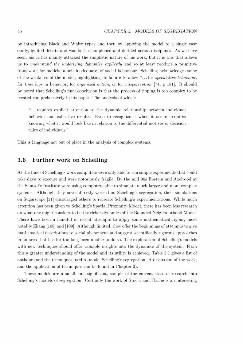
46 CHAPTER 3. MODELS OF SEGREGATION
by introducing Black and White types and then by applying the model to a single case
study, ignited debate and was both championed and derided across disciplines. As we have
seen, his critics mainly attacked the simplistic nature of his work, but it is this that allows
us to understand the underlying dynamics explicitly and so at least produce a primitive
framework for models, albeit inadequate, of social behaviour. Schelling acknowledges some
of the weakness of the model, highlighting its failure to allow “. . . for speculative behaviour,
for time lags in behavior, for organized action, or for misperception”[74, p 181]. It should
be noted that Schelling’s final conclusion is that the process of tipping is too complex to be
treated comprehensively in his paper. The analysis of which:
“. . . requires explicit attention to the dynamic relationship between individual
behavior and collective results. Even to recognize it when it occurs requires
knowing what it would look like in relation to the di↵erential motives or decision
rules of individuals.”
This is language not out of place in the analysis of complex systems.
3.6 Further work on Schelling
At the time of Schelling’s work computers were only able to run simple experiments that could
take days to execute and were notoriously fragile. By the mid 90s Epstein and Axelrood at
the Santa Fe Institute were using computers able to simulate much larger and more complex
systems. Although they never directly worked on Schelling’s segregation, their simulations
on Sugarscape [31] encouraged others to recreate Schelling’s experimentations. While much
attention has been given to Schelling’s Spatial Proximity Model, there has been less research
on what one might consider to be the richer dynamics of the Bounded Neighbourhood Model.
There have been a handful of recent attempts to apply some mathematical rigour, most
notably Zhang [108] and [109]. Although limited, they o↵er the beginnings of attempts to give
mathematical descriptions to social phenomena and suggest scientifically rigorous approaches
in an area that has for too long been unable to do so. The exploration of Schelling’s models
with new techniques should o↵er valuable insights into the dynamics of the system. From
this a greater understanding of the model and its utility is achieved. Table 3.1 gives a list of
authours and the techniques used to model Schelling’s segregation. A discussion of the work,
and the application of techniques can be found in Chapter 2).
These models are a small, but significant, sample of the current state of research into
Schelling’s models of segregation. Certainly the work of Stocia and Flache is an interesting
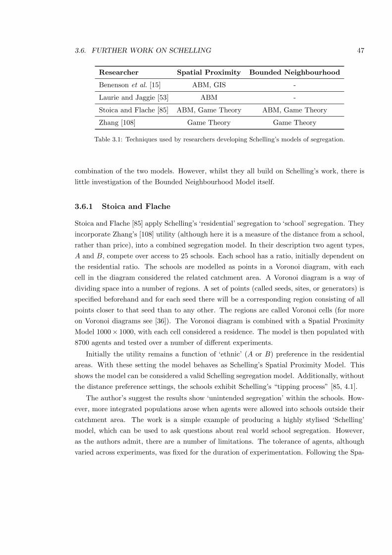
3.6. FURTHER WORK ON SCHELLING 47
Researcher Spatial Proximity Bounded Neighbourhood
Benenson et al. [15] ABM, GIS -
Laurie and Jaggie [53] ABM -
Stoica and Flache [85] ABM, Game Theory ABM, Game Theory
Zhang [108] Game Theory Game Theory
Table 3.1: Techniques used by researchers developing Schelling’s models of segregation.
combination of the two models. However, whilst they all build on Schelling’s work, there is
little investigation of the Bounded Neighbourhood Model itself.
3.6.1 Stoica and Flache
Stoica and Flache [85] apply Schelling’s ‘residential’ segregation to ‘school’ segregation. They
incorporate Zhang’s [108] utility (although here it is a measure of the distance from a school,
rather than price), into a combined segregation model. In their description two agent types,
A and B, compete over access to 25 schools. Each school has a ratio, initially dependent on
the residential ratio. The schools are modelled as points in a Voronoi diagram, with each
cell in the diagram considered the related catchment area. A Voronoi diagram is a way of
dividing space into a number of regions. A set of points (called seeds, sites, or generators) is
specified beforehand and for each seed there will be a corresponding region consisting of all
points closer to that seed than to any other. The regions are called Voronoi cells (for more
on Voronoi diagrams see [36]). The Voronoi diagram is combined with a Spatial Proximity
Model 1000⇥ 1000, with each cell considered a residence. The model is then populated with
8700 agents and tested over a number of di↵erent experiments.
Initially the utility remains a function of ‘ethnic’ (A or B) preference in the residential
areas. With these setting the model behaves as Schelling’s Spatial Proximity Model. This
shows the model can be considered a valid Schelling segregation model. Additionally, without
the distance preference settings, the schools exhibit Schelling’s “tipping process” [85, 4.1].
The author’s suggest the results show ‘unintended segregation’ within the schools. How-
ever, more integrated populations arose when agents were allowed into schools outside their
catchment area. The work is a simple example of producing a highly stylised ‘Schelling’
model, which can be used to ask questions about real world school segregation. However,
as the authors admit, there are a number of limitations. The tolerance of agents, although
varied across experiments, was fixed for the duration of experimentation. Following the Spa-

48 CHAPTER 3. MODELS OF SEGREGATION
tial Proximity Model, each agent had an identical tolerance, no ideas of a distribution of
tolerance were discussed. In addition the model has a deterministic choice function, which
the authors admit, should be replaced with a random utility function akin to Zhang’s [108].
The attempts of the authours’, to apply the model to ‘real world’ situations, is hindered
by the lack of understanding into some of the workings of Schelling’s model. In addition by
combining the two models, it is di�cult to analyse the e↵ects of space on the Bounded Neigh-
bourhood Model. To gain further insights, it will be important to build a valid simulation of
Schelling’s Bounded Neighbourhood Model. From this process, some of the mechanics that
drive to model should be exposed.
Chapter 4
Methodology
In examining and developing Schelling’s Bounded Neighbourhood model it is important to
build a solid, defendable framework in which simulations can be developed and run. The
simulations can then be used to test hypotheses about the model. Since models are unable
to capture all the information within complex systems, there is a need for some level of
abstraction. This abstraction will exclude information. In addition, since emergent properties
of the system are being sought and so not explicitly included in the simulation, it can be
di�cult to tell if an emergent behaviour is a result of the property being sought, or just
created by a bug in the code (or model).1 Therefore it is important that the development
follows a systematic and scientifically sound process. The CoSMoS process has been widely
used to model a number of real-world phenomena (see Section 4.3). However, the application
of the process to a social model is a novel approach. The CoSMoS process provides a rigorous
framework o↵ering a solid foundation necessary for methodological soundness.
4.1 Verification
Verification and validation of computer simulations are important ways of checking for cor-
rectness of computer code (in this case a software simulation). Despite thirty years of research
in the area, their use is far from widespread. This is possibly because software development
in science is typically ‘hacked’, rather than ‘engineered’in a formal sense. While the ideas
were not intended for complex systems, they are certainly a useful tool for improving models
and their simulations.
Ideas verification and validation of computational accuracy were first defined by Schlesinger,
1Whilst this can also be considered an emergent behaviour, we believe it is not the class of emergence wedesire.
49
50 CHAPTER 4. METHODOLOGY
calling verification the: “. . . substantiation that a computerized model represents a concep-
tual model within specified limits of accuracy” [78]. This initial description was simplified by
Sargent who argues verification can be defined as: “. . . ensuring that the computer program
of the computerized model and its implementation are correct” [72]. Thus, the verification
process is designed to show that the software is internally consistent and correct. This is
usually achieved through rigorous testing, using procedures that have been developed and
refined in the software engineering field. As with any program there is a need for stringent
checks of protocols and structures, to make sure the language is correct; additionally, the
program needs to be as bug-free as possible. Tests are done using techniques such as correct-
ness proofs and structured walk-throughs [72]. Rigorous testing of software has developed a
number of techniques that can be implemented, including running a trace, entering variables
incorrectly, reprogramming critical components and many others [103]. The fact that the
verification process is an established knowledge based on years of research means that it can
be applied with some confidence.
4.1.1 Prediction
Popper suggests that the power of physics comes from verification through prediction [67].
This is almost impossible with complex systems and certainly not to the degree of accuracy de-
manded by physics and mathematics. For this reason the issue of prediction is contentious in
the field of complexity. Epstein [30] argues that prediction is not the only reason for modelling
complex systems and believes that an understanding of the system is much more important.
Thompson and Derr [87] counter that with this understanding there must be an ability to
predict, citing apparent abilities to predict earthquakes and tra�c jams. Troitzsch [88] o↵ers
a good summation of the arguments and suggests that without defining what is meant by
a prediction the argument is flawed. Using Thompson and Derr’s arguments about plate
tectonics, Troitzsch o↵ers three di↵erent types of prediction:
1. Which kinds of behaviour can be expected [from a system like this] under arbitrarily
given parameter combinations and initial conditions?
2. Which kind of behaviour will a given target system (whose parameters and previous
states may or may not have been precisely measured) display in the near future?
3. Which state will the target system reach in the near future, again given parameters and
previous states which may or may not have been precisely measured?
(a) Which are the expected value and the confidence interval around the expected
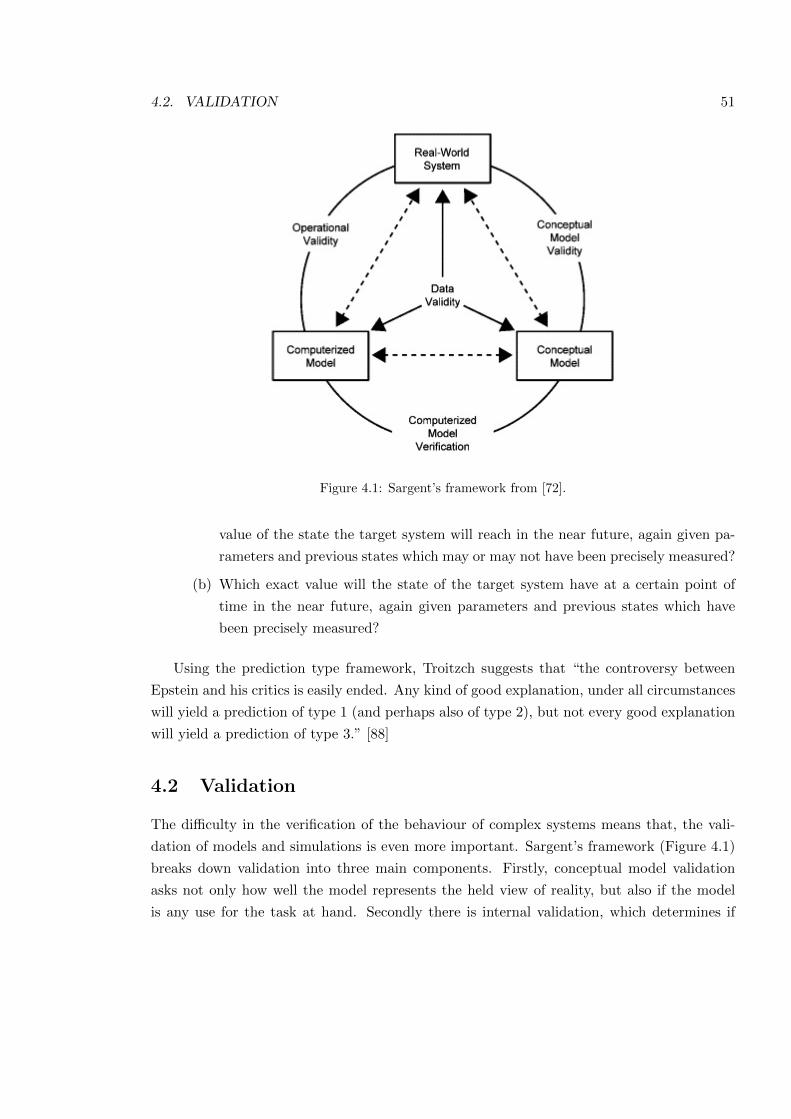
4.2. VALIDATION 51
Figure 4.1: Sargent’s framework from [72].
value of the state the target system will reach in the near future, again given pa-
rameters and previous states which may or may not have been precisely measured?
(b) Which exact value will the state of the target system have at a certain point of
time in the near future, again given parameters and previous states which have
been precisely measured?
Using the prediction type framework, Troitzch suggests that “the controversy between
Epstein and his critics is easily ended. Any kind of good explanation, under all circumstances
will yield a prediction of type 1 (and perhaps also of type 2), but not every good explanation
will yield a prediction of type 3.” [88]
4.2 Validation
The di�culty in the verification of the behaviour of complex systems means that, the vali-
dation of models and simulations is even more important. Sargent’s framework (Figure 4.1)
breaks down validation into three main components. Firstly, conceptual model validation
asks not only how well the model represents the held view of reality, but also if the model
is any use for the task at hand. Secondly there is internal validation, which determines if
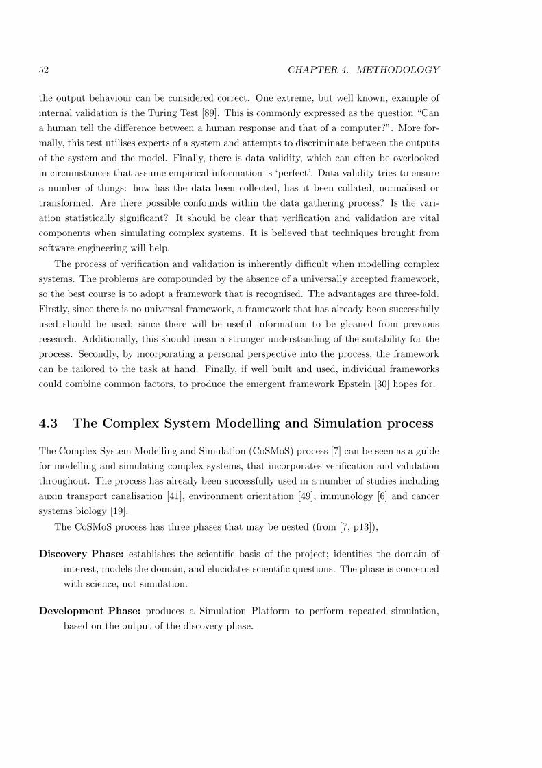
52 CHAPTER 4. METHODOLOGY
the output behaviour can be considered correct. One extreme, but well known, example of
internal validation is the Turing Test [89]. This is commonly expressed as the question “Can
a human tell the di↵erence between a human response and that of a computer?”. More for-
mally, this test utilises experts of a system and attempts to discriminate between the outputs
of the system and the model. Finally, there is data validity, which can often be overlooked
in circumstances that assume empirical information is ‘perfect’. Data validity tries to ensure
a number of things: how has the data been collected, has it been collated, normalised or
transformed. Are there possible confounds within the data gathering process? Is the vari-
ation statistically significant? It should be clear that verification and validation are vital
components when simulating complex systems. It is believed that techniques brought from
software engineering will help.
The process of verification and validation is inherently di�cult when modelling complex
systems. The problems are compounded by the absence of a universally accepted framework,
so the best course is to adopt a framework that is recognised. The advantages are three-fold.
Firstly, since there is no universal framework, a framework that has already been successfully
used should be used; since there will be useful information to be gleaned from previous
research. Additionally, this should mean a stronger understanding of the suitability for the
process. Secondly, by incorporating a personal perspective into the process, the framework
can be tailored to the task at hand. Finally, if well built and used, individual frameworks
could combine common factors, to produce the emergent framework Epstein [30] hopes for.
4.3 The Complex System Modelling and Simulation process
The Complex System Modelling and Simulation (CoSMoS) process [7] can be seen as a guide
for modelling and simulating complex systems, that incorporates verification and validation
throughout. The process has already been successfully used in a number of studies including
auxin transport canalisation [41], environment orientation [49], immunology [6] and cancer
systems biology [19].
The CoSMoS process has three phases that may be nested (from [7, p13]),
Discovery Phase: establishes the scientific basis of the project; identifies the domain of
interest, models the domain, and elucidates scientific questions. The phase is concerned
with science, not simulation.
Development Phase: produces a Simulation Platform to perform repeated simulation,
based on the output of the discovery phase.
4.3. THE COMPLEX SYSTEM MODELLING AND SIMULATION PROCESS 53
Figure 2.1: Relationships among products (rectangles) and the domain of interest. Ar-rows give a sense of the information flow involved in development of products. TheResearch Context is the central and unavoidable product, on which all other productsare dependent
Domain Model: encapsulates understanding of appropriate aspects of the domaininto explicit domain understanding. The domain model focuses on the scientificunderstanding; no simulation implementation details are considered.
Platform Model: comprises design and implementation models for the simulation plat-form, based on the domain model and research context.
Simulation Platform : encodes the platform model into a software and hardware plat-form upon which simulations can be performed.
Results Model : encapsulates the understanding that results from simulation: thesimulation platform behaviour, results of data collection and observations of sim-ulation runs. Note that the way that the domain model captures the relevant un-derstanding of the domain is mirrored by the way that the results model capturesunderstanding of the simulation platform.
Figure 2.1 summarises the relationships among the CoSMoS products, showing howinformation flows between the products.
The CoSMoS process iterates through the three phases until a stopping condition ismet. At each stage, the products may be updated, though it is also possible to simply
14
Figure 4.2: The Complex Systems Modelling and Simulation (CoSMoS) process from [7].
Exploration Phase: uses the Simulation Platform resulting from the development phase
to explore the scientific questions established during the discovery phase.
In recognition of the challenges involved in understanding and recreating complex behaviours,
these phases are not constrained; they can be used iteratively or alternatively, as best suits
the problem being considered.
The CoSMoS process identifies products that represent artefacts that are created and
modified during these phases. By separating out these artefacts, the process is able to clarify
the verification and validation of the model, simulation and results. This separation allows
problems to be identified at specific points in the process. The artefacts as defined in [7, p13]
are:
The Research Context: captures the overall scientific research context of the project. In-
cluding motivation for doing the research, the questions to be addressed by the Simu-
lation Platform, and requirements for validation and evaluation. The research context
is discussed in Chapter 2, as well as in the introduction to each experiment (Chapter
6, 7, 8 and 9).
The Domain Model: encapsulates understanding of appropriate aspects of the domain
into explicit domain understanding. The Domain Model focuses on the scientific un-
derstanding; no simulation implementation details are considered. The Domain Model
54 CHAPTER 4. METHODOLOGY
is described in Chapter 5.1.
Platform Model: comprises design and implementation models for the Simulation Plat-
form, based on the Domain Model and research context. The Platform Model can
be UML, pseudo-code or any style that describes the model as it will be run, by the
Simulation Platform. This allows the highlighting of possible artefacts arising from the
code. The simplicity of Schelling’s Bounded Neighbourhood Model means it is easily
described using pseudo-code in Chapter 5.2.
Simulation Platform: encodes the Platform Model into a software and hardware platform
upon which simulations can be performed. This process is a straightforward process of
translating the pseudo-code in Chapter 5.2 into Netlogo [3].
Results Model: encapsulates the understanding that results from simulation: the Simula-
tion Platform behaviour, results of data collection and observations of simulation runs.
Note that the way that the Domain Model captures the relevant understanding of the
domain is mirrored by the way that the Results Model captures understanding of the
Simulation Platform. The results are analysed using the Wilcoxon-Mann-Whitney U
test. This nonparametric test is introduced in Chapter 4.4.
The problems discussed by Epstein [30] and Thompson & Derr [87] rather than being
systemic, can be addressed at di↵erent stages of the modelling process. Thompson and Derr’s
arguments of verification are based on a simple comparison of their Results Model with actual
results. This is problematic on at least a couple of levels. Firstly, if their results di↵er from
expected they will be unable to gauge where the ‘fault’ lies. Secondly, and more importantly,
if their results are as expected, they will still be unable to validate the model or the simulation
individually, since it is quite possible an inaccuracy in the model is nullified by an error in the
simulation and produces the ‘correct’ result. This holistic approach to modelling a complex
system renders one blind to where anomalies could lie. Without knowing where the problem
is, one might have to start again from scratch.
By following the CoSMoS process an important distinction is made, not only between the
model and the software that implements the model in the simulation, but also between the
results from the simulation and any results from the ‘real’ world domain. By breaking down
the process of modelling, it can be seen that the arguments of Epstein [30], Thompson &
Derr [87] and Troitzsch [88] have arisen from an attempt to move straight from the domain
to the simulation. Without considering a Domain Model one can see their problems are
exacerbated by the attempts to build simulations directly from the domain.
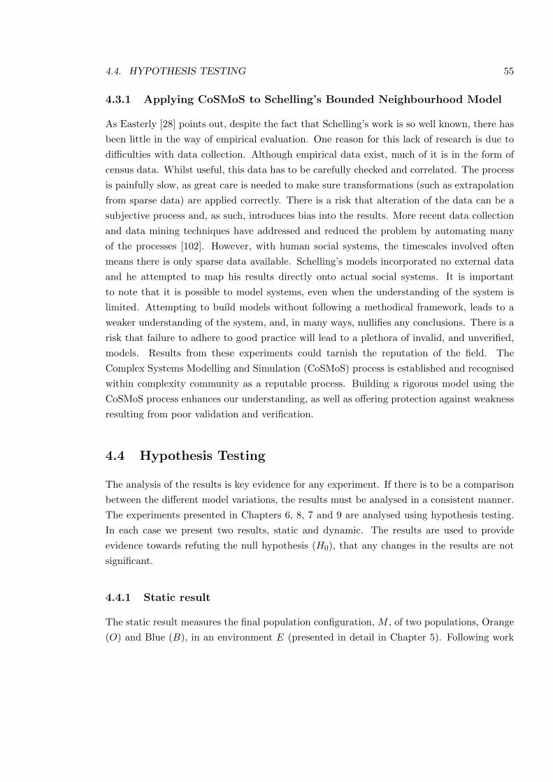
4.4. HYPOTHESIS TESTING 55
4.3.1 Applying CoSMoS to Schelling’s Bounded Neighbourhood Model
As Easterly [28] points out, despite the fact that Schelling’s work is so well known, there has
been little in the way of empirical evaluation. One reason for this lack of research is due to
di�culties with data collection. Although empirical data exist, much of it is in the form of
census data. Whilst useful, this data has to be carefully checked and correlated. The process
is painfully slow, as great care is needed to make sure transformations (such as extrapolation
from sparse data) are applied correctly. There is a risk that alteration of the data can be a
subjective process and, as such, introduces bias into the results. More recent data collection
and data mining techniques have addressed and reduced the problem by automating many
of the processes [102]. However, with human social systems, the timescales involved often
means there is only sparse data available. Schelling’s models incorporated no external data
and he attempted to map his results directly onto actual social systems. It is important
to note that it is possible to model systems, even when the understanding of the system is
limited. Attempting to build models without following a methodical framework, leads to a
weaker understanding of the system, and, in many ways, nullifies any conclusions. There is a
risk that failure to adhere to good practice will lead to a plethora of invalid, and unverified,
models. Results from these experiments could tarnish the reputation of the field. The
Complex Systems Modelling and Simulation (CoSMoS) process is established and recognised
within complexity community as a reputable process. Building a rigorous model using the
CoSMoS process enhances our understanding, as well as o↵ering protection against weakness
resulting from poor validation and verification.
4.4 Hypothesis Testing
The analysis of the results is key evidence for any experiment. If there is to be a comparison
between the di↵erent model variations, the results must be analysed in a consistent manner.
The experiments presented in Chapters 6, 8, 7 and 9 are analysed using hypothesis testing.
In each case we present two results, static and dynamic. The results are used to provide
evidence towards refuting the null hypothesis (H0), that any changes in the results are not
significant.
4.4.1 Static result
The static result measures the final population configuration, M , of two populations, Orange
(O) and Blue (B), in an environment E (presented in detail in Chapter 5). Following work
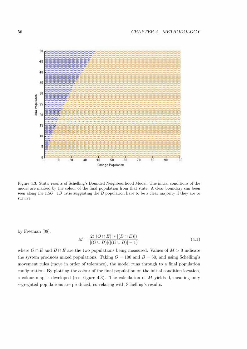
56 CHAPTER 4. METHODOLOGY
Figure 4.3: Static results of Schelling’s Bounded Neighbourhood Model. The initial conditions of themodel are marked by the colour of the final population from that state. A clear boundary can beenseen along the 1.5O : 1B ratio suggesting the B population have to be a clear majority if they are tosurvive.
by Freeman [38],
M =2(|(O \ E)| ⇤ |(B \ E)|)
|(O [B)|(|(O [B)|� 1), (4.1)
where O \ E and B \ E are the two populations being measured. Values of M > 0 indicate
the system produces mixed populations. Taking O = 100 and B = 50, and using Schelling’s
movement rules (move in order of tolerance), the model runs through to a final population
configuration. By plotting the colour of the final population on the initial condition location,
a colour map is developed (see Figure 4.3). The calculation of M yields 0, meaning only
segregated populations are produced, correlating with Schelling’s results.
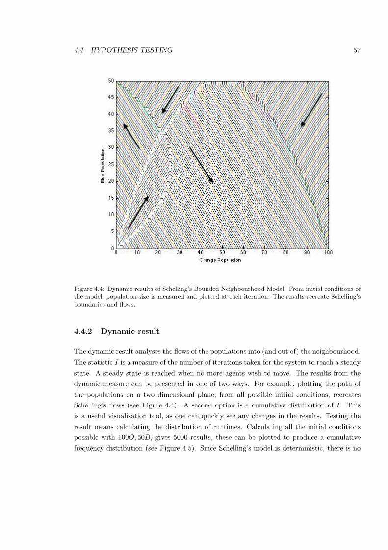
4.4. HYPOTHESIS TESTING 57
Figure 4.4: Dynamic results of Schelling’s Bounded Neighbourhood Model. From initial conditions ofthe model, population size is measured and plotted at each iteration. The results recreate Schelling’sboundaries and flows.
4.4.2 Dynamic result
The dynamic result analyses the flows of the populations into (and out of) the neighbourhood.
The statistic I is a measure of the number of iterations taken for the system to reach a steady
state. A steady state is reached when no more agents wish to move. The results from the
dynamic measure can be presented in one of two ways. For example, plotting the path of
the populations on a two dimensional plane, from all possible initial conditions, recreates
Schelling’s flows (see Figure 4.4). A second option is a cumulative distribution of I. This
is a useful visualisation tool, as one can quickly see any changes in the results. Testing the
result means calculating the distribution of runtimes. Calculating all the initial conditions
possible with 100O, 50B, gives 5000 results, these can be plotted to produce a cumulative
frequency distribution (see Figure 4.5). Since Schelling’s model is deterministic, there is no
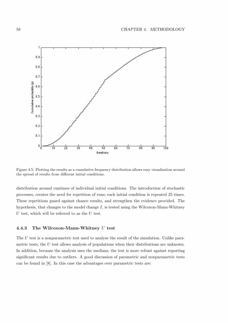
58 CHAPTER 4. METHODOLOGY
Figure 4.5: Plotting the results as a cumulative frequency distribution allows easy visualisation aroundthe spread of results from di↵erent initial conditions.
distribution around runtimes of individual initial conditions. The introduction of stochastic
processes, creates the need for repetition of runs; each initial condition is repeated 25 times.
These repetitions guard against chance results, and strengthen the evidence provided. The
hypothesis, that changes to the model change I, is tested using the Wilcoxon-Mann-Whitney
U test, which will be referred to as the U test.
4.4.3 The Wilcoxon-Mann-Whitney U test
The U test is a nonparametric test used to analyse the result of the simulation. Unlike para-
metric tests, the U test allows analysis of populations when their distributions are unknown.
In addition, because the analysis uses the medians, the test is more robust against reporting
significant results due to outliers. A good discussion of parametric and nonparametric tests
can be found in [8]. In this case the advantages over parametric tests are:
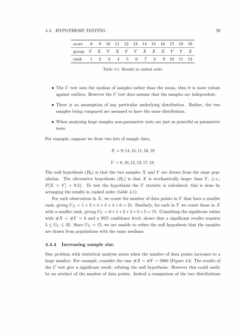
4.4. HYPOTHESIS TESTING 59
score 8 9 10 11 12 13 14 15 16 17 18 19
group Y X Y X Y Y X X X Y Y X
rank 1 2 3 4 5 6 7 8 9 10 11 12
Table 4.1: Results in ranked order
• The U test uses the median of samples rather than the mean, thus it is more robust
against outliers. However the U test does assume that the samples are independent.
• There is no assumption of any particular underlying distribution. Rather, the two
samples being compared are assumed to have the same distribution.
• When analysing large samples non-parametric tests are just as powerful as parametric
tests.
For example, suppose we draw two lots of sample data,
X = 9, 14, 15, 11, 16, 19
Y = 8, 10, 12, 13, 17, 18.
The null hypothesis (H0) is that the two samples X and Y are drawn from the same pop-
ulation. The alternative hypothesis (H1) is that X is stochastically larger than Y , (i.e.,
P [X > Y ] > 0.5). To test the hypothesis the U statistic is calculated, this is done by
arranging the results in ranked order (table 4.1).
For each observation in X, we count the number of data points in Y that have a smaller
rank, giving UX = 1 + 2 + 4 + 4 + 4 + 6 = 21. Similarly, for each in Y we count those in X
with a smaller rank, giving UY = 0+1+2+2+5+5 = 15. Consulting the significant tables
with #X = #Y = 6 and a 95% confidence level, shows that a significant results requires
5 UY 32. Since UY = 15, we are unable to refute the null hypothesis that the samples
are drawn from populations with the same medians.
4.4.4 Increasing sample size
One problem with statistical analysis arises when the number of data points increases to a
large number. For example, consider the case #X = #Y = 5000 (Figure 4.6. The results of
the U test give a significant result, refuting the null hypothesis. However this could easily
be an artefact of the number of data points. Indeed a comparison of the two distributions
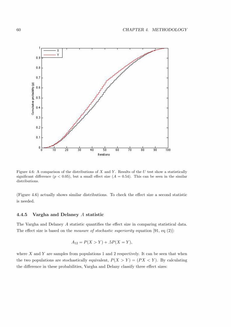
60 CHAPTER 4. METHODOLOGY
Figure 4.6: A comparison of the distributions of X and Y . Results of the U test show a statisticallysignificant di↵erence (p < 0.05), but a small e↵ect size (A = 0.54). This can be seen in the similardistributions.
(Figure 4.6) actually shows similar distributions. To check the e↵ect size a second statistic
is needed.
4.4.5 Vargha and Delaney A statistic
The Vargha and Delaney A statistic quantifies the e↵ect size in comparing statistical data.
The e↵ect size is based on the measure of stochastic superiority equation [91, eq (2)]:
A12 = P (X > Y ) + .5P (X = Y ),
where X and Y are samples from populations 1 and 2 respectively. It can be seen that when
the two populations are stochastically equivalent, P (X > Y ) = (PX < Y ). By calculating
the di↵erence in these probabilities, Vargha and Delany classify three e↵ect sizes:
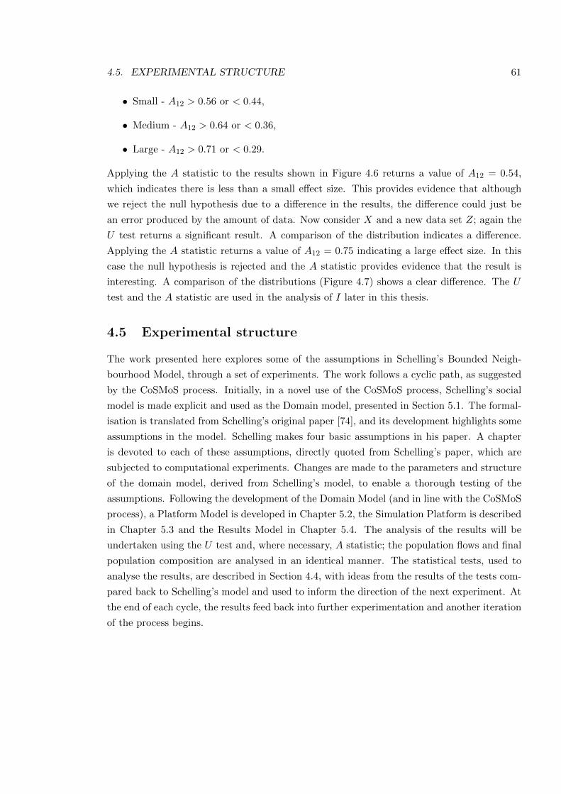
4.5. EXPERIMENTAL STRUCTURE 61
• Small - A12 > 0.56 or < 0.44,
• Medium - A12 > 0.64 or < 0.36,
• Large - A12 > 0.71 or < 0.29.
Applying the A statistic to the results shown in Figure 4.6 returns a value of A12 = 0.54,
which indicates there is less than a small e↵ect size. This provides evidence that although
we reject the null hypothesis due to a di↵erence in the results, the di↵erence could just be
an error produced by the amount of data. Now consider X and a new data set Z; again the
U test returns a significant result. A comparison of the distribution indicates a di↵erence.
Applying the A statistic returns a value of A12 = 0.75 indicating a large e↵ect size. In this
case the null hypothesis is rejected and the A statistic provides evidence that the result is
interesting. A comparison of the distributions (Figure 4.7) shows a clear di↵erence. The U
test and the A statistic are used in the analysis of I later in this thesis.
4.5 Experimental structure
The work presented here explores some of the assumptions in Schelling’s Bounded Neigh-
bourhood Model, through a set of experiments. The work follows a cyclic path, as suggested
by the CoSMoS process. Initially, in a novel use of the CoSMoS process, Schelling’s social
model is made explicit and used as the Domain model, presented in Section 5.1. The formal-
isation is translated from Schelling’s original paper [74], and its development highlights some
assumptions in the model. Schelling makes four basic assumptions in his paper. A chapter
is devoted to each of these assumptions, directly quoted from Schelling’s paper, which are
subjected to computational experiments. Changes are made to the parameters and structure
of the domain model, derived from Schelling’s model, to enable a thorough testing of the
assumptions. Following the development of the Domain Model (and in line with the CoSMoS
process), a Platform Model is developed in Chapter 5.2, the Simulation Platform is described
in Chapter 5.3 and the Results Model in Chapter 5.4. The analysis of the results will be
undertaken using the U test and, where necessary, A statistic; the population flows and final
population composition are analysed in an identical manner. The statistical tests, used to
analyse the results, are described in Section 4.4, with ideas from the results of the tests com-
pared back to Schelling’s model and used to inform the direction of the next experiment. At
the end of each cycle, the results feed back into further experimentation and another iteration
of the process begins.
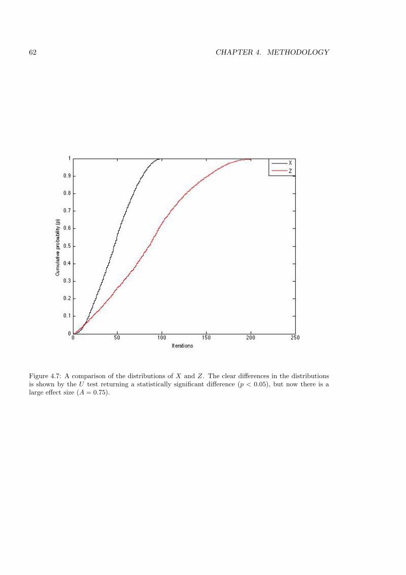
62 CHAPTER 4. METHODOLOGY
Figure 4.7: A comparison of the distributions of X and Z. The clear di↵erences in the distributionsis shown by the U test returning a statistically significant di↵erence (p < 0.05), but now there is alarge e↵ect size (A = 0.75).
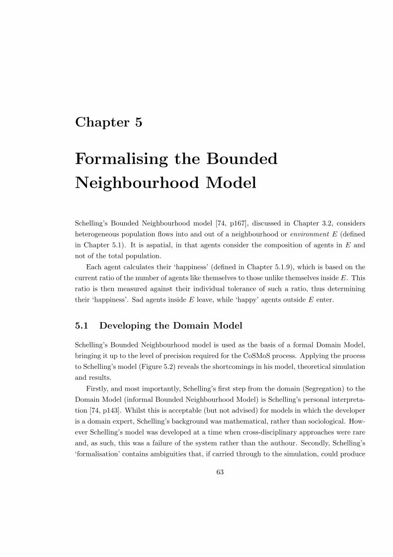
Chapter 5
Formalising the Bounded
Neighbourhood Model
Schelling’s Bounded Neighbourhood model [74, p167], discussed in Chapter 3.2, considers
heterogeneous population flows into and out of a neighbourhood or environment E (defined
in Chapter 5.1). It is aspatial, in that agents consider the composition of agents in E and
not of the total population.
Each agent calculates their ‘happiness’ (defined in Chapter 5.1.9), which is based on the
current ratio of the number of agents like themselves to those unlike themselves inside E. This
ratio is then measured against their individual tolerance of such a ratio, thus determining
their ‘happiness’. Sad agents inside E leave, while ‘happy’ agents outside E enter.
5.1 Developing the Domain Model
Schelling’s Bounded Neighbourhood model is used as the basis of a formal Domain Model,
bringing it up to the level of precision required for the CoSMoS process. Applying the process
to Schelling’s model (Figure 5.2) reveals the shortcomings in his model, theoretical simulation
and results.
Firstly, and most importantly, Schelling’s first step from the domain (Segregation) to the
Domain Model (informal Bounded Neighbourhood Model) is Schelling’s personal interpreta-
tion [74, p143]. Whilst this is acceptable (but not advised) for models in which the developer
is a domain expert, Schelling’s background was mathematical, rather than sociological. How-
ever Schelling’s model was developed at a time when cross-disciplinary approaches were rare
and, as such, this was a failure of the system rather than the authour. Secondly, Schelling’s
‘formalisation’ contains ambiguities that, if carried through to the simulation, could produce
63
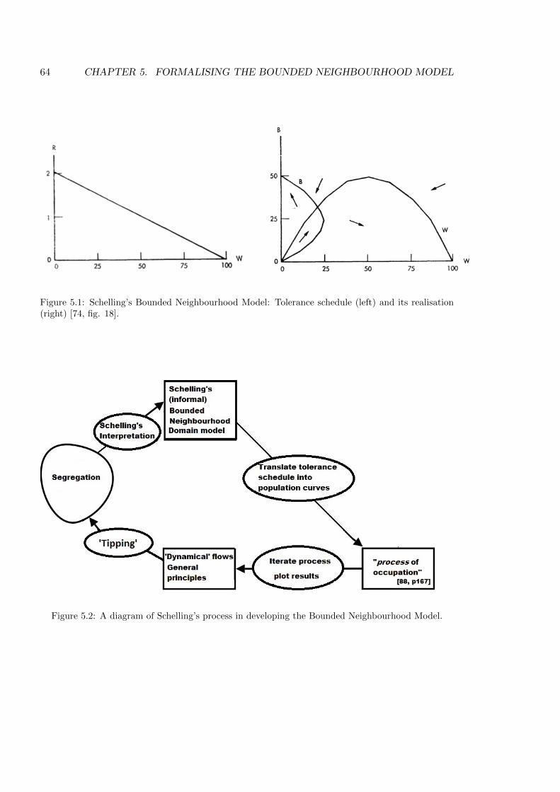
64 CHAPTER 5. FORMALISING THE BOUNDED NEIGHBOURHOOD MODEL
Figure 5.1: Schelling’s Bounded Neighbourhood Model: Tolerance schedule (left) and its realisation(right) [74, fig. 18].
Figure 5.2: A diagram of Schelling’s process in developing the Bounded Neighbourhood Model.
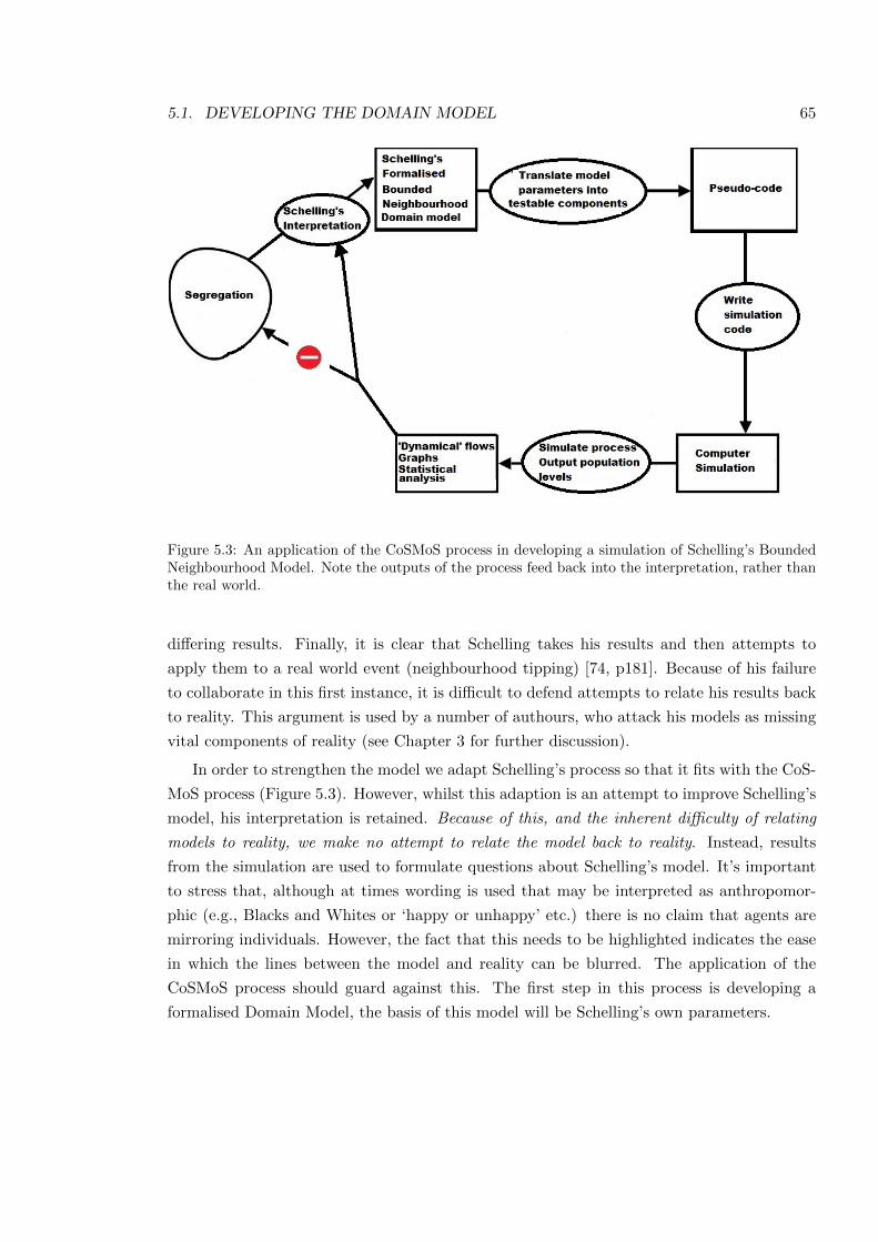
5.1. DEVELOPING THE DOMAIN MODEL 65
Figure 5.3: An application of the CoSMoS process in developing a simulation of Schelling’s BoundedNeighbourhood Model. Note the outputs of the process feed back into the interpretation, rather thanthe real world.
di↵ering results. Finally, it is clear that Schelling takes his results and then attempts to
apply them to a real world event (neighbourhood tipping) [74, p181]. Because of his failure
to collaborate in this first instance, it is di�cult to defend attempts to relate his results back
to reality. This argument is used by a number of authours, who attack his models as missing
vital components of reality (see Chapter 3 for further discussion).
In order to strengthen the model we adapt Schelling’s process so that it fits with the CoS-
MoS process (Figure 5.3). However, whilst this adaption is an attempt to improve Schelling’s
model, his interpretation is retained. Because of this, and the inherent di�culty of relating
models to reality, we make no attempt to relate the model back to reality. Instead, results
from the simulation are used to formulate questions about Schelling’s model. It’s important
to stress that, although at times wording is used that may be interpreted as anthropomor-
phic (e.g., Blacks and Whites or ‘happy or unhappy’ etc.) there is no claim that agents are
mirroring individuals. However, the fact that this needs to be highlighted indicates the ease
in which the lines between the model and reality can be blurred. The application of the
CoSMoS process should guard against this. The first step in this process is developing a
formalised Domain Model, the basis of this model will be Schelling’s own parameters.
66 CHAPTER 5. FORMALISING THE BOUNDED NEIGHBOURHOOD MODEL
Neighbourhood. Schelling describes this as a particular bounded area that is preferred
to any alternative (where possible in this thesis we avoid terminology with spatial
connotations). He gives as examples membership of a club or participation in a job.
“A person is either inside it or outside it” [74, p167].
Colour Ratio. It is measured against agents’ tolerance to calculate the state of the agent.
“Absolute numbers do not matter, only ratios.” [74, p167]
Tolerance. A limit that, once reached, triggers agent movement.
“He will reside in it unless the percentage of residents of opposite color exceeds some
limit. Each person, black or white, has his own limit. (’Tolerance,’ we shall occasionally
call it.) If a person’s limit is exceeded in this area he will go someplace else” [74, p167].
Process of occupation. Population movement into and out of the system. This is the
process Schelling was most interested in,
“What we can do is look at the process by which the area becomes occupied” [74, p167].
Following these, Benenson [15] suggests some “standard settings” for a Schelling segrega-
tion model. Although based on Schelling’s Spatial Proximity Model (see Chapter 3.1), the set-
tings (set out below) are used as the basis for the formalisation of the Bounded Neighbourhood
Model. The major di↵erences between the models are the agents’ consideration/definition
of neighbourhood and their tolerance. Although both use the same concept of Neighbour-
hood Ratio to determine ‘happiness’ (defined below), the models explore di↵erent dynamics.
The Spatial Proximity Model looks at the dynamics within a neighbourhood, whereas the
Bounded Neighbourhood Model explores the e↵ects of agents’ movement into and out of a
neighbourhood. Agent ‘happiness’ is measured by comparing the tolerance of the agent with
the current ratio of the neighbourhood. If the neighbourhood ratio is above the level of the
agent’s tolerance then the agent is deemed ‘unhappy’ and will attempt to move.
The Bounded Neighbourhood Model parameter settings are described below:
The Environment. The environment is defined as a global neighbourhood, in which agents
are either inside or outside.
Neighbourhood Ratio. This is the number of agents of other type compared to the number
of own type inside the neighbourhood.
Agent Location. Agents are either inside or outside of the neighbourhood.
Agent Tolerance. Agents’ level of tolerance of the ratio of their neighbourhood. Unlike the
Spatial Proximity Model, where agents all have the same tolerance, here the agents’
5.1. DEVELOPING THE DOMAIN MODEL 67
tolerance is defined as a cumulative straight line schedule (Figure 5.1). Individual agents
of the same type have a di↵erent level of tolerance. Two agents of di↵erent type could
have the same level of tolerance.
Agent Dynamics. The ‘unhappy’ Bounded Neighbourhood Model agents (within the neigh-
bourhood) remove themselves one by one, starting with the most ‘unhappy’ of the pop-
ulation. If there are agents outside the system who would be ‘happy’ to be inside, they
move in one at a time starting with the most ‘happy’.
By using an aspatial model, Schelling is able to extend the model beyond spatial grids. This
allows the encapsulation of groups that are not necessarily spatially linked. The model can
be described by the following characteristics.
5.1.1 The Environment
The model has two aspatial regions (sets of agents), the neighbourhood E (agents ‘inside’)
and its complement E⇤ (agents ‘outside’).
5.1.2 Agent Location
Agents are located in E or in E⇤. Agents’ decisions are based solely on the composition of
E.
5.1.3 Agent Type
Schelling’s model explores ideas of segregation with two distinct populations distributed inside
the neighbourhoods E. The populations consist of two types or sets W and B (it is natural
to think that B represents the set of ‘blacks’ and W the set of ‘whites’):
TYPE = {B,W}. (5.1)
Clearly this can be generalised to any number of types:
TYPE = {T1, T2, . . . , Tn} ; n � 2. (5.2)
5.1.4 Agent numbers
The set of all agents is B[W = E[E⇤ (all agents are either inside or outside); their number
is |B| + |W |. The number of agents in B and in E (the number of black agents inside)
68 CHAPTER 5. FORMALISING THE BOUNDED NEIGHBOURHOOD MODEL
is |(B \ E)|, the number of agents in W and in E (the number of white agents inside) is
|(W \ E)|. In his initial experiment Schelling [74, fig.18] chooses |B| = 50, |W | = 100.
5.1.5 Ratio of the two populations
Schelling defines the Ratio RWB for B to be the number of white agents inside compared to
the number of black agents inside. This can be formalised as
RWB =|(W \ E)|
|(B \ E)|(5.3)
and the ratio RBW for W is the reciprocal of RWB,
RBW =|(B \ E)|
|(W \ E)|, (5.4)
provided that the denominators do not vanish. The case when they do vanish is discussed in
Chapter 5.1.6.
In the general case, Rij is the ratio of the number of all agents of type j to the number
of type i:
Rij =1
|(Ti \ E)|
X
j 6=i
|(Tj \ E)|, (5.5)
provided Ti \E 6= ;. Here we also assume that all other types are equally weighted (equally
disliked); a more complicated model could include a weighting factor zij(i 6= j) for each type
relative to each other type.
5.1.6 The tolerance schedule and definition of ⌧
Schelling assigns each agent a tolerance, which we denote by ⌧ . The tolerance of an agent
w is thus w(⌧) and that of an agent b is b(⌧). These tolerances are defined by a schedule
comprising a straight line cumulative frequency distribution1 (see equations (5.6) and (5.7)
below). Here we quote the relevant passage from [74, p.168], with our parenthetical additions
of specific model parameters and values:
We can take the total of whites to be 100 [|W | = 100]. Suppose that the median
white [w50] is willing to live with blacks in equal numbers [has ⌧ = 1], so that 50
among our 100 whites [w1 to w50] will abide a ratio of black to white of 1.0 or
greater. The most tolerant white [w1] can abide a black-white ratio of two to one
1Strictly speaking a cumulative distribution function must be monotonic increasing; and would be if theaxis was “intolerance”.
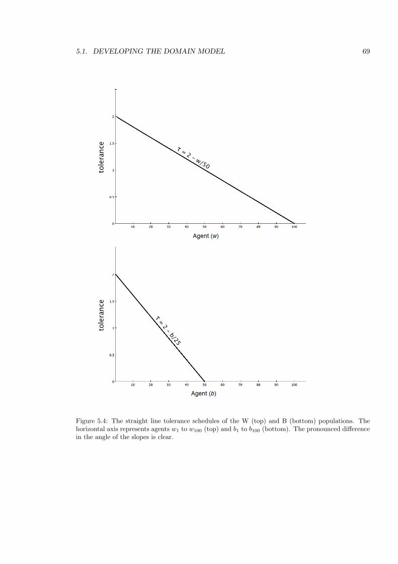
5.1. DEVELOPING THE DOMAIN MODEL 69
Figure 5.4: The straight line tolerance schedules of the W (top) and B (bottom) populations. Thehorizontal axis represents agents w1 to w100 (top) and b1 to b100 (bottom). The pronounced di↵erencein the angle of the slopes is clear.
70 CHAPTER 5. FORMALISING THE BOUNDED NEIGHBOURHOOD MODEL
[has ⌧ = 2], that is, is willing to be in a one-third minority; and the least tolerant
white [w100] cannot stand the presence of any blacks [has ⌧ = 0]. The cumulative
distribution of tolerances for a white population will then appear as in the top
of Figure 18 [our Figure 5.1]. It is a straight line with intercept at a ratio of 2.0
on the vertical axis and intercept on the horizontal axis at the 100 whites who
comprise the white population.
In other words, the W population is ordered according to tolerance, and giving them a
numerical identification according to its position in the line. The first (most tolerant) agent
(w1) has ⌧ = ⌧max = 2, the last (least tolerant) agent (w100) has ⌧ = 0, and the intermediate
agents have ⌧ values defined by a linear interpolation. This is shown in Figure 5.4. The hor-
izontal axis represents the numerical identification w1 �w100 of agents, in order of tolerance.
The vertical axis ⌧ represents the maximum ratio an agent will tolerate. The mathematical
formulation gives the linear equation
wn(⌧) = 2�wn
50, (5.6)
so that, for instance, w100 has tolerance ⌧ = 0 (Figure 5.4). However there is a problem
concerning the origin. It is clear from Schelling’s sentence
“The most tolerant white . . . is willing to be in a one-third minority;” [74, p.168],
he assumes that w1 has a tolerance ⌧ = 2 in contradiction to (5.6), where when w0(> w1) has
tolerance ⌧ = 2. The formula can be reconciled with the above sentence either by altering
the end points or the slope. For instance the linear schedule can be chosen to pass through
the points (1, 2) and (100, 0) in which case the slope is �2/99 and the tolerance ⌧ is given by
wn(⌧) = �
2wn
99+
200
99.
Nevertheless we will continue to use equation (5.6) for ease of comparison with Schelling’s
paper (noting that the relatively small discrepancy does not a↵ect the conclusions drawn).
Schelling’s initial model also uses a similar tolerance schedule with the same maximal
tolerance ⌧ = 2 but with |B = 50| and with slope �1/25. This gives the lower of the two
diagram shown in Figure 5.4. The mathematical formulation gives the linear equation
bn(⌧) = 2�bn25
, (5.7)
so that, for instance, agent b50 has ⌧ = 0 (again, the same problems with the origin, as
mentioned earlier, arise and are ignored).
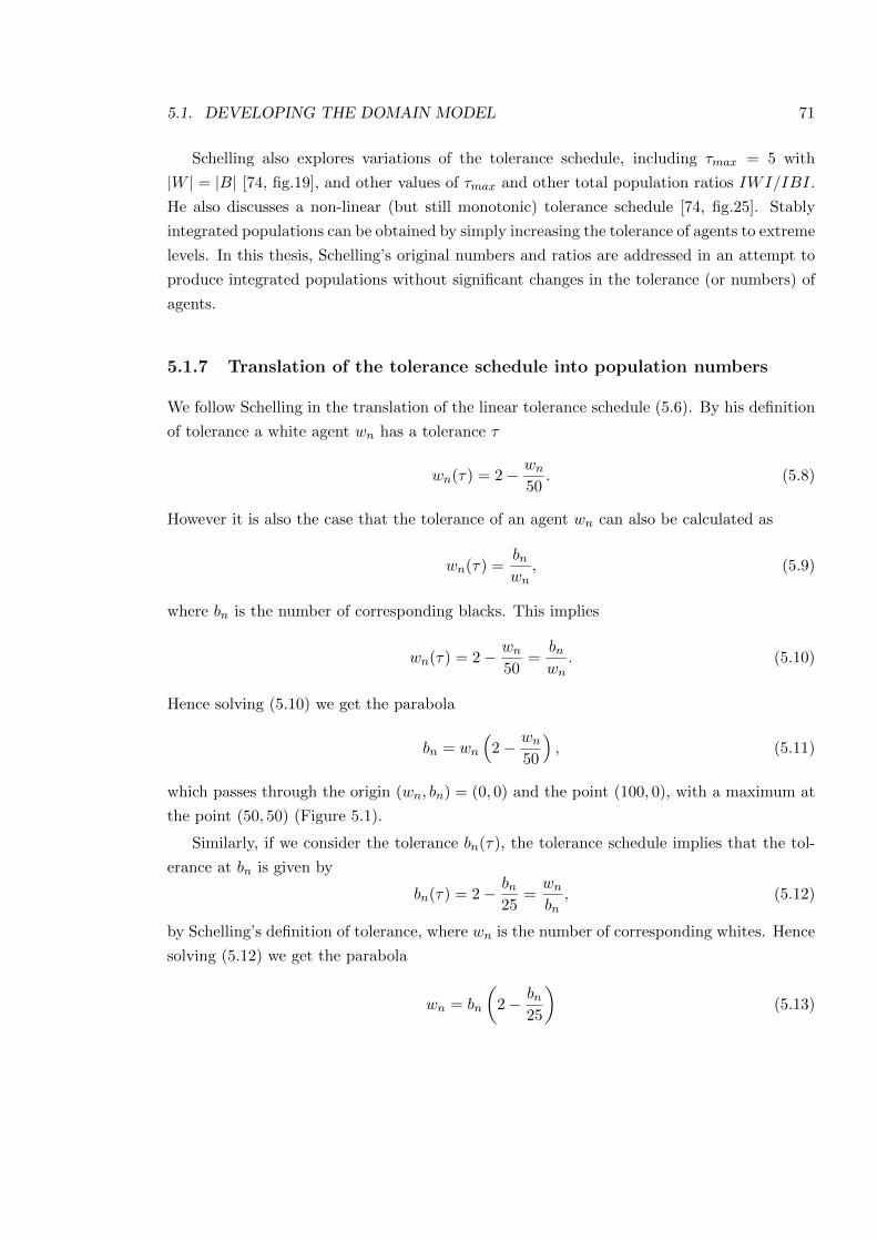
5.1. DEVELOPING THE DOMAIN MODEL 71
Schelling also explores variations of the tolerance schedule, including ⌧max = 5 with
|W | = |B| [74, fig.19], and other values of ⌧max and other total population ratios IWI/IBI.
He also discusses a non-linear (but still monotonic) tolerance schedule [74, fig.25]. Stably
integrated populations can be obtained by simply increasing the tolerance of agents to extreme
levels. In this thesis, Schelling’s original numbers and ratios are addressed in an attempt to
produce integrated populations without significant changes in the tolerance (or numbers) of
agents.
5.1.7 Translation of the tolerance schedule into population numbers
We follow Schelling in the translation of the linear tolerance schedule (5.6). By his definition
of tolerance a white agent wn has a tolerance ⌧
wn(⌧) = 2�wn
50. (5.8)
However it is also the case that the tolerance of an agent wn can also be calculated as
wn(⌧) =bnwn
, (5.9)
where bn is the number of corresponding blacks. This implies
wn(⌧) = 2�wn
50=
bnwn
. (5.10)
Hence solving (5.10) we get the parabola
bn = wn
⇣2�
wn
50
⌘, (5.11)
which passes through the origin (wn, bn) = (0, 0) and the point (100, 0), with a maximum at
the point (50, 50) (Figure 5.1).
Similarly, if we consider the tolerance bn(⌧), the tolerance schedule implies that the tol-
erance at bn is given by
bn(⌧) = 2�bn25
=wn
bn, (5.12)
by Schelling’s definition of tolerance, where wn is the number of corresponding whites. Hence
solving (5.12) we get the parabola
wn = bn
✓2�
bn25
◆(5.13)
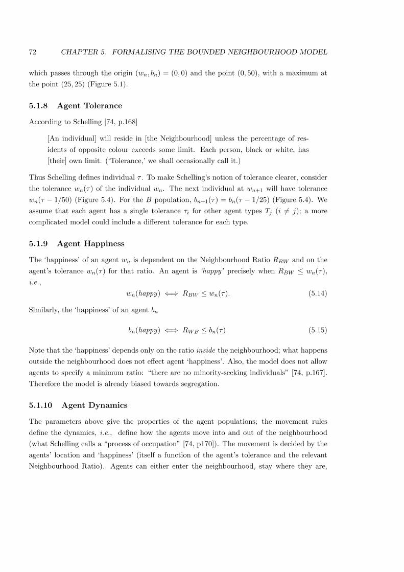
72 CHAPTER 5. FORMALISING THE BOUNDED NEIGHBOURHOOD MODEL
which passes through the origin (wn, bn) = (0, 0) and the point (0, 50), with a maximum at
the point (25, 25) (Figure 5.1).
5.1.8 Agent Tolerance
According to Schelling [74, p.168]
[An individual] will reside in [the Neighbourhood] unless the percentage of res-
idents of opposite colour exceeds some limit. Each person, black or white, has
[their] own limit. (‘Tolerance,’ we shall occasionally call it.)
Thus Schelling defines individual ⌧ . To make Schelling’s notion of tolerance clearer, consider
the tolerance wn(⌧) of the individual wn. The next individual at wn+1 will have tolerance
wn(⌧ � 1/50) (Figure 5.4). For the B population, bn+1(⌧) = bn(⌧ � 1/25) (Figure 5.4). We
assume that each agent has a single tolerance ⌧i for other agent types Tj (i 6= j); a more
complicated model could include a di↵erent tolerance for each type.
5.1.9 Agent Happiness
The ‘happiness’ of an agent wn is dependent on the Neighbourhood Ratio RBW and on the
agent’s tolerance wn(⌧) for that ratio. An agent is ‘happy’ precisely when RBW wn(⌧),
i.e.,
wn(happy) () RBW wn(⌧). (5.14)
Similarly, the ‘happiness’ of an agent bn
bn(happy) () RWB bn(⌧). (5.15)
Note that the ‘happiness’ depends only on the ratio inside the neighbourhood; what happens
outside the neighbourhood does not e↵ect agent ‘happiness’. Also, the model does not allow
agents to specify a minimum ratio: “there are no minority-seeking individuals” [74, p.167].
Therefore the model is already biased towards segregation.
5.1.10 Agent Dynamics
The parameters above give the properties of the agent populations; the movement rules
define the dynamics, i.e., define how the agents move into and out of the neighbourhood
(what Schelling calls a “process of occupation” [74, p170]). The movement is decided by the
agents’ location and ‘happiness’ (itself a function of the agent’s tolerance and the relevant
Neighbourhood Ratio). Agents can either enter the neighbourhood, stay where they are,
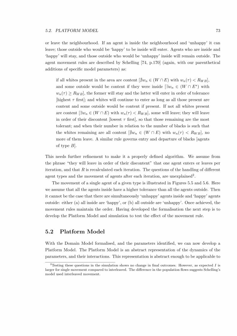
5.2. PLATFORM MODEL 73
or leave the neighbourhood. If an agent is inside the neighbourhood and ‘unhappy’ it can
leave; those outside who would be ‘happy’ to be inside will enter. Agents who are inside and
‘happy’ will stay, and those outside who would be ‘unhappy’ inside will remain outside. The
agent movement rules are described by Schelling [74, p.170] (again, with our parenthetical
additions of specific model parameters) as:
if all whites present in the area are content [@wn 2 (W \E) with wn(⌧) < RWB],
and some outside would be content if they were inside [9wn 2 (W \ E⇤) with
wn(⌧) � RWB], the former will stay and the latter will enter in order of tolerance
[highest ⌧ first]; and whites will continue to enter as long as all those present are
content and some outside would be content if present. If not all whites present
are content [9wn 2 (W \E) with wn(⌧) < RWB], some will leave; they will leave
in order of their discontent [lowest ⌧ first], so that those remaining are the most
tolerant; and when their number in relation to the number of blacks is such that
the whites remaining are all content [@wn 2 (W \ E) with wn(⌧) < RWB], no
more of them leave. A similar rule governs entry and departure of blacks [agents
of type B].
This needs further refinement to make it a properly defined algorithm. We assume from
the phrase “they will leave in order of their discontent” that one agent enters or leaves per
iteration, and that R is recalculated each iteration. The questions of the handling of di↵erent
agent types and the movement of agents after each iteration, are unexplained2.
The movement of a single agent of a given type is illustrated in Figures 5.5 and 5.6. Here
we assume that all the agents inside have a higher tolerance than all the agents outside. Then
it cannot be the case that there are simultaneously ‘unhappy’ agents inside and ‘happy’ agents
outside: either (a) all inside are ‘happy’, or (b) all outside are ‘unhappy’. Once achieved, the
movement rules maintain the order. Having developed the formalisation the next step is to
develop the Platform Model and simulation to test the e↵ect of the movement rule.
5.2 Platform Model
With the Domain Model formalised, and the parameters identified, we can now develop a
Platform Model. The Platform Model is an abstract representation of the dynamics of the
parameters, and their interactions. This representation is abstract enough to be applicable to
2Testing these questions in the simulation shows no change in final outcomes. However, as expected I islarger for single movement compared to interleaved. The di↵erence in the population flows suggests Schelling’smodel used interleaved movement.
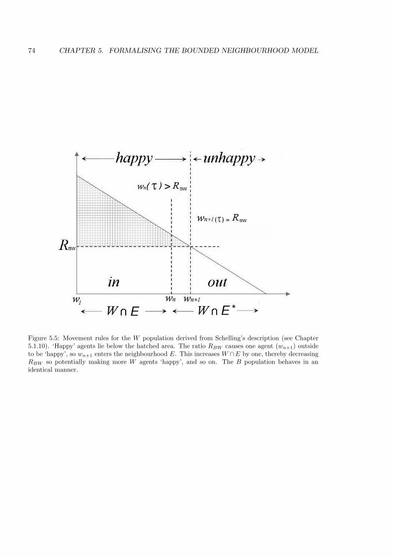
74 CHAPTER 5. FORMALISING THE BOUNDED NEIGHBOURHOOD MODEL
Figure 5.5: Movement rules for the W population derived from Schelling’s description (see Chapter5.1.10). ‘Happy’ agents lie below the hatched area. The ratio RBW causes one agent (wn+1) outsideto be ‘happy’, so wn+1 enters the neighbourhood E. This increases W \E by one, thereby decreasingRBW so potentially making more W agents ‘happy’, and so on. The B population behaves in anidentical manner.
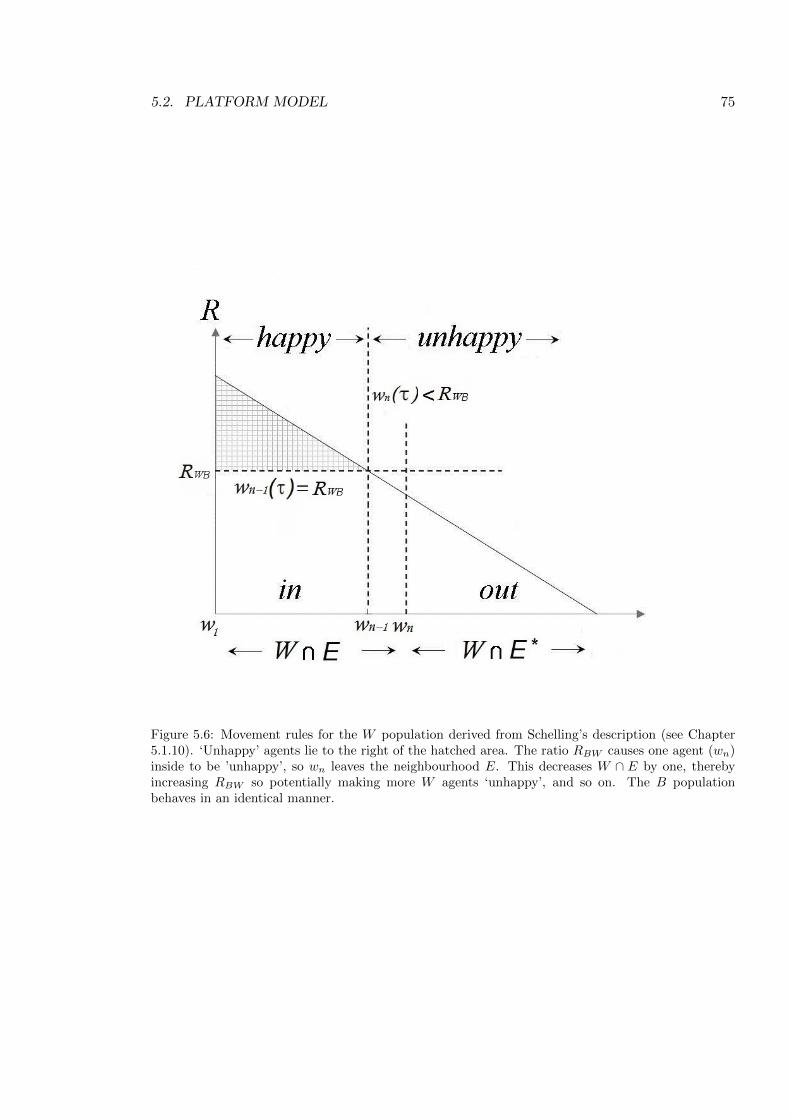
5.2. PLATFORM MODEL 75
Figure 5.6: Movement rules for the W population derived from Schelling’s description (see Chapter5.1.10). ‘Unhappy’ agents lie to the right of the hatched area. The ratio RBW causes one agent (wn)inside to be ’unhappy’, so wn leaves the neighbourhood E. This decreases W \ E by one, therebyincreasing RBW so potentially making more W agents ‘unhappy’, and so on. The B populationbehaves in an identical manner.
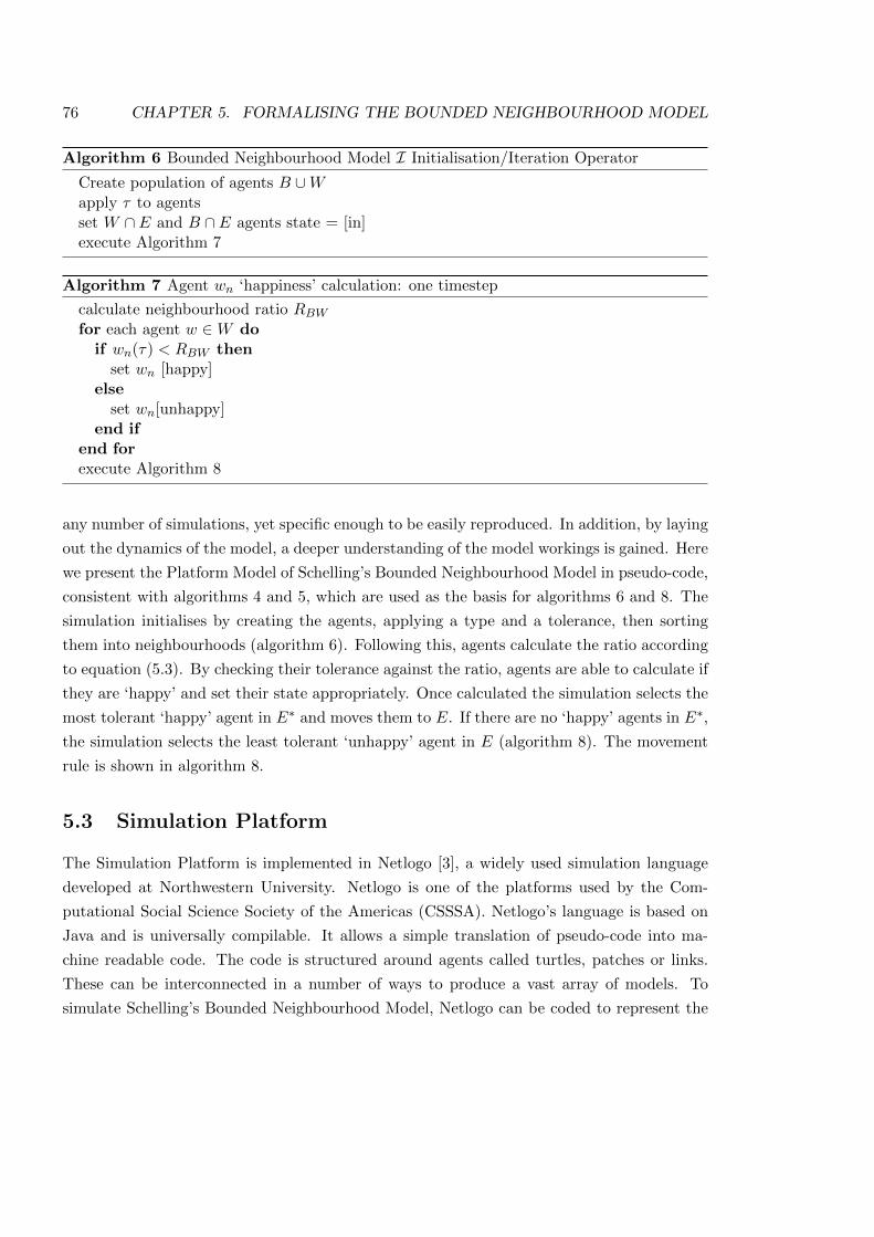
76 CHAPTER 5. FORMALISING THE BOUNDED NEIGHBOURHOOD MODEL
Algorithm 6 Bounded Neighbourhood Model I Initialisation/Iteration Operator
Create population of agents B [Wapply ⌧ to agentsset W \ E and B \ E agents state = [in]execute Algorithm 7
Algorithm 7 Agent wn ‘happiness’ calculation: one timestep
calculate neighbourhood ratio RBW
for each agent w 2 W doif wn(⌧) < RBW then
set wn [happy]else
set wn[unhappy]end if
end forexecute Algorithm 8
any number of simulations, yet specific enough to be easily reproduced. In addition, by laying
out the dynamics of the model, a deeper understanding of the model workings is gained. Here
we present the Platform Model of Schelling’s Bounded Neighbourhood Model in pseudo-code,
consistent with algorithms 4 and 5, which are used as the basis for algorithms 6 and 8. The
simulation initialises by creating the agents, applying a type and a tolerance, then sorting
them into neighbourhoods (algorithm 6). Following this, agents calculate the ratio according
to equation (5.3). By checking their tolerance against the ratio, agents are able to calculate if
they are ‘happy’ and set their state appropriately. Once calculated the simulation selects the
most tolerant ‘happy’ agent in E⇤ and moves them to E. If there are no ‘happy’ agents in E⇤,
the simulation selects the least tolerant ‘unhappy’ agent in E (algorithm 8). The movement
rule is shown in algorithm 8.
5.3 Simulation Platform
The Simulation Platform is implemented in Netlogo [3], a widely used simulation language
developed at Northwestern University. Netlogo is one of the platforms used by the Com-
putational Social Science Society of the Americas (CSSSA). Netlogo’s language is based on
Java and is universally compilable. It allows a simple translation of pseudo-code into ma-
chine readable code. The code is structured around agents called turtles, patches or links.
These can be interconnected in a number of ways to produce a vast array of models. To
simulate Schelling’s Bounded Neighbourhood Model, Netlogo can be coded to represent the
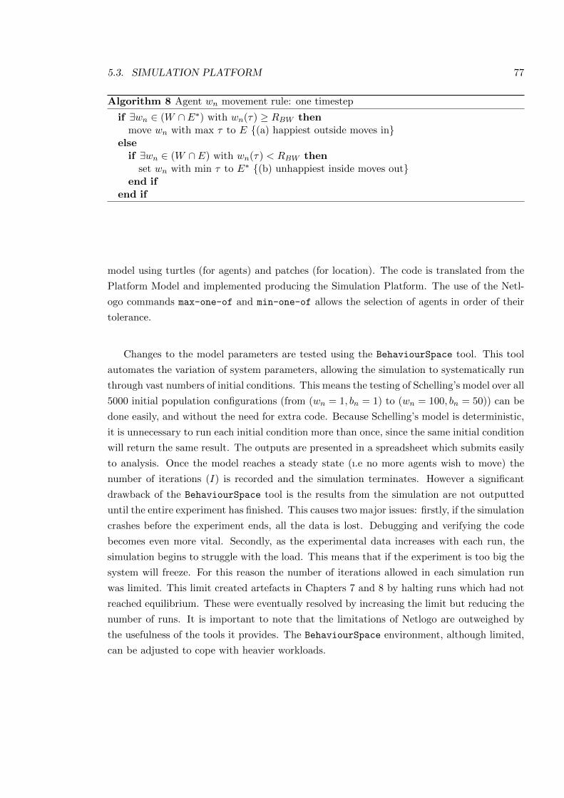
5.3. SIMULATION PLATFORM 77
Algorithm 8 Agent wn movement rule: one timestep
if 9wn 2 (W \ E⇤) with wn(⌧) � RBW thenmove wn with max ⌧ to E {(a) happiest outside moves in}
elseif 9wn 2 (W \ E) with wn(⌧) < RBW then
set wn with min ⌧ to E⇤{(b) unhappiest inside moves out}
end ifend if
model using turtles (for agents) and patches (for location). The code is translated from the
Platform Model and implemented producing the Simulation Platform. The use of the Netl-
ogo commands max-one-of and min-one-of allows the selection of agents in order of their
tolerance.
Changes to the model parameters are tested using the BehaviourSpace tool. This tool
automates the variation of system parameters, allowing the simulation to systematically run
through vast numbers of initial conditions. This means the testing of Schelling’s model over all
5000 initial population configurations (from (wn = 1, bn = 1) to (wn = 100, bn = 50)) can be
done easily, and without the need for extra code. Because Schelling’s model is deterministic,
it is unnecessary to run each initial condition more than once, since the same initial condition
will return the same result. The outputs are presented in a spreadsheet which submits easily
to analysis. Once the model reaches a steady state (ı.e no more agents wish to move) the
number of iterations (I) is recorded and the simulation terminates. However a significant
drawback of the BehaviourSpace tool is the results from the simulation are not outputted
until the entire experiment has finished. This causes two major issues: firstly, if the simulation
crashes before the experiment ends, all the data is lost. Debugging and verifying the code
becomes even more vital. Secondly, as the experimental data increases with each run, the
simulation begins to struggle with the load. This means that if the experiment is too big the
system will freeze. For this reason the number of iterations allowed in each simulation run
was limited. This limit created artefacts in Chapters 7 and 8 by halting runs which had not
reached equilibrium. These were eventually resolved by increasing the limit but reducing the
number of runs. It is important to note that the limitations of Netlogo are outweighed by
the usefulness of the tools it provides. The BehaviourSpace environment, although limited,
can be adjusted to cope with heavier workloads.
78 CHAPTER 5. FORMALISING THE BOUNDED NEIGHBOURHOOD MODEL
5.4 Results Model
In keeping with the CoSMoS process described in Chapter 4.1, the results of the simula-
tion will be measured and analysed using hypothesis testing (see Chapter 4.4). To recover
Schelling’s flows, the population level will be recorded at each iteration and plotted on a
two dimensional diagram, identical to Schelling’s results. One iteration is defined as the
movement of one agent, as described in Chapter 5.1.10. A run terminates when no more
agents wish to move, with I being the number of iterations taken to reach that point. The
configuration of the final population is calculated using M (see Equation (4.1)). In later
experiments, these results will be used to test the hypothesis, that changing the parameters
of the model changes the results.
5.4.1 Validation
By comparing the results of the simulation with Schelling’s results, evidence is provided
towards validation of the simulation. Because Schelling’s movement rules were imprecise,
we are unable to measure the number of iterations the model takes to reach a steady state.
Instead the flows of the populations are plotted from each initial condition. Figure 5.7 shows
a comparison of these simulation flows, against Schelling’s diagrammatical flows. The flows of
the simulation mimic Schelling’s results, the parabolas clearly identify identical boundaries.
5.5 Summary
This chapter has presented a formalisation of Schelling’s Bounded Neighbourhood Model
within the CoSMoS framework (Section 5.1), from which a Netlogo simulation has been
developed (Section 5.2). The formalisation and development of a simulation allows for the
testing of the e↵ects of a number of possible parameter values of the system. This initial
work has focused on the formalisation of the model and the development of a simulation. The
analysis of results (Section 5.4) show that the simulation replicates Schelling’s population
dynamics. However there is a small ambiguity, the B population in Schelling’s model appear,
from his diagrams, to exit the neighbourhood more slowly than the simulation results. This
is an interesting point, and is explored further in Chapter 8.
Schelling’s Bounded Neighbourhood Model can be considered a highly simplistic first
step in the understanding of how prejudices can e↵ect the movement of populations into
and out of ‘neighbourhoods’. The simplicity of the model allows a full understanding of
the dynamics that are driving it but, unfortunately, those dynamics are unable to produce
any ‘interesting’ results. However it is possible to use this model as a basis for a more
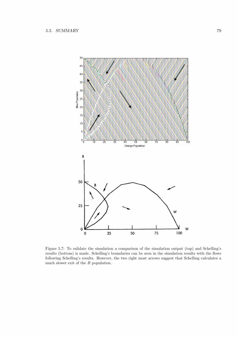
5.5. SUMMARY 79
Figure 5.7: To validate the simulation a comparison of the simulation output (top) and Schelling’sresults (bottom) is made. Schelling’s boundaries can be seen in the simulation results with the flowsfollowing Schelling’s results. However, the two right most arrows suggest that Schelling calculates amuch slower exit of the B population.
80 CHAPTER 5. FORMALISING THE BOUNDED NEIGHBOURHOOD MODEL
complex model by modifying or adding appropriate features which allow the modified model
to be tested systematically. Indeed, by developing a valid simulation of Schelling’s Bounded
Neighbourhood model, it is now possible to ask questions of the model, such as the existence of
stable equilibria, that have previously been di�cult to answer. This is done for the formalised
Bounded Neighbourhood model to test the robustness of the assumptions made by Schelling
(listed below) and carried out in Chapters 6, 7, 8 and 9.
Whose move is it anyway? The movement of the agents depends on their knowledge of
every other agent’s ‘happiness’. By changing the movement rule, Chapter 6, explores
the e↵ect of randomly choosing agents who wish to move, rather than moving by order.
Who do you know? The fact that agents have complete knowledge of the neighbourhood.
This is tested in Chapter 7, in which agents sample the neighbourhood to calculate
their ‘happiness’.
Should I stay, or should I go? This refers to the assumption that agents move as soon
as they are ‘unhappy’. This is tested in Chapter 8, where it is assumed their decision
to move is based on a level of ‘happiness’ derived from the neighbourhood ratio.
Friends and neighbours. The fact that all agents are treated equally within type. By
recasting Schelling’s Bounded Neighbourhood Model as a network in Chapter 9, we
explore the e↵ects of social ties within the neighbourhood.
At each step the formalisation of Schelling’s Bounded Neighbourhood Model is adjusted
to develop a simulation to test these assumptions. The work begins with the movement of
the agents and what e↵ect their order of movement has on the results.
Chapter 6
Whose move is it anyway?
“It is the least tolerant whites that move out first, and the most tolerant that
move in first, and similarly for blacks.” [74, p168]
6.1 Introduction
The formalisation of the Bounded Neighbourhood Model has highlighted a testable assump-
tion. The movement of the agents is dependent on their complete knowledge of the ‘happiness’
of every other agent, as the least ‘happy’ inside (or the most ‘happy’ outside) moves first. By
removing this knowledge, we can test the hypothesis that the movement of agents, ordered
by their level of tolerance, has no significant e↵ect on the results. In this chapter, we apply
a variation to the agents’ movement rule, and test it against Schelling’s rule. Thus, we have
two movement rules:
1. Agents move one at a time according to level of tolerance (as described by Schelling).
2. Agents wishing to move are chosen randomly.
6.2 Hypothesis
The hypotheses tests the e↵ects of changing the movement rule on the model. We o↵er the
null hypothesis (H0) that changing the movement will have no e↵ect on the outcome of the
simulation. This is tested using two measures, static and dynamic (discussed in Section 4.4).
81
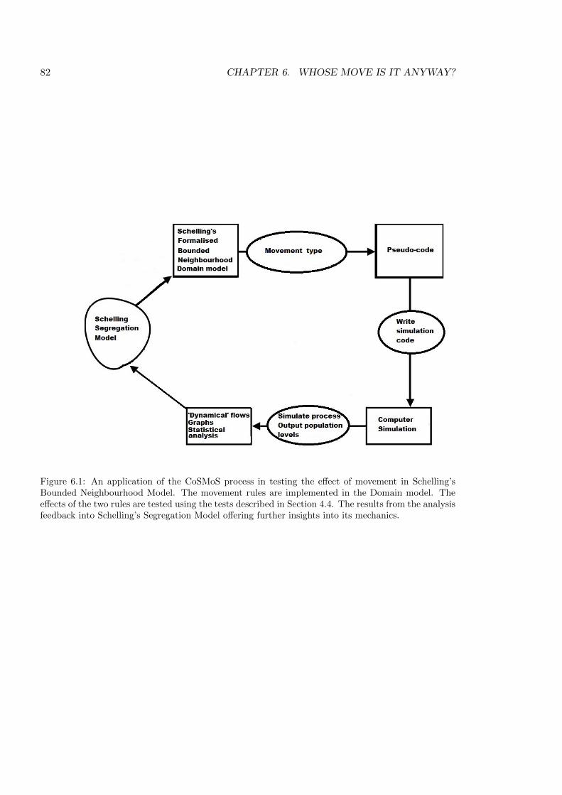
82 CHAPTER 6. WHOSE MOVE IS IT ANYWAY?
Figure 6.1: An application of the CoSMoS process in testing the e↵ect of movement in Schelling’sBounded Neighbourhood Model. The movement rules are implemented in the Domain model. Thee↵ects of the two rules are tested using the tests described in Section 4.4. The results from the analysisfeedback into Schelling’s Segregation Model o↵ering further insights into its mechanics.
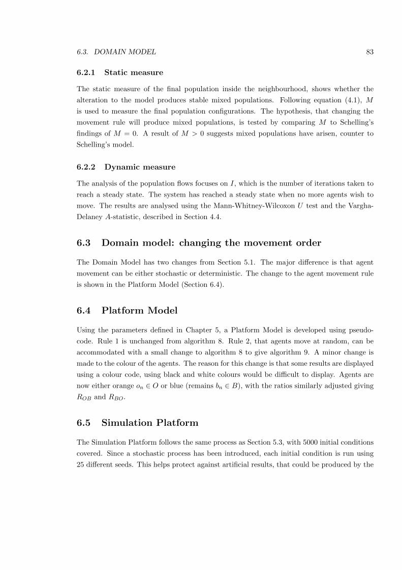
6.3. DOMAIN MODEL 83
6.2.1 Static measure
The static measure of the final population inside the neighbourhood, shows whether the
alteration to the model produces stable mixed populations. Following equation (4.1), M
is used to measure the final population configurations. The hypothesis, that changing the
movement rule will produce mixed populations, is tested by comparing M to Schelling’s
findings of M = 0. A result of M > 0 suggests mixed populations have arisen, counter to
Schelling’s model.
6.2.2 Dynamic measure
The analysis of the population flows focuses on I, which is the number of iterations taken to
reach a steady state. The system has reached a steady state when no more agents wish to
move. The results are analysed using the Mann-Whitney-Wilcoxon U test and the Vargha-
Delaney A-statistic, described in Section 4.4.
6.3 Domain model: changing the movement order
The Domain Model has two changes from Section 5.1. The major di↵erence is that agent
movement can be either stochastic or deterministic. The change to the agent movement rule
is shown in the Platform Model (Section 6.4).
6.4 Platform Model
Using the parameters defined in Chapter 5, a Platform Model is developed using pseudo-
code. Rule 1 is unchanged from algorithm 8. Rule 2, that agents move at random, can be
accommodated with a small change to algorithm 8 to give algorithm 9. A minor change is
made to the colour of the agents. The reason for this change is that some results are displayed
using a colour code, using black and white colours would be di�cult to display. Agents are
now either orange on 2 O or blue (remains bn 2 B), with the ratios similarly adjusted giving
ROB and RBO.
6.5 Simulation Platform
The Simulation Platform follows the same process as Section 5.3, with 5000 initial conditions
covered. Since a stochastic process has been introduced, each initial condition is run using
25 di↵erent seeds. This helps protect against artificial results, that could be produced by the
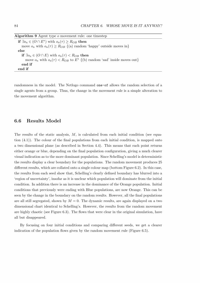
84 CHAPTER 6. WHOSE MOVE IS IT ANYWAY?
Algorithm 9 Agent type o movement rule: one timestep
if 9on 2 (O \ E⇤) with on(⌧) � ROB thenmove on with on(⌧) � ROB {(a) random ‘happy’ outside moves in}
elseif 9on 2 (O \ E) with on(⌧) < ROB then
move on with on(⌧) < ROB to E⇤{(b) random ‘sad’ inside moves out}
end ifend if
randomness in the model. The Netlogo command one-of allows the random selection of a
single agents from a group. Thus, the change in the movement rule is a simple alteration to
the movement algorithm.
6.6 Results Model
The results of the static analysis, M , is calculated from each initial condition (see equa-
tion (4.1)). The colour of the final populations from each initial condition, is mapped onto
a two dimensional plane (as described in Section 4.4). This means that each point returns
either orange or blue, depending on the final population configuration, giving a much clearer
visual indication as to the more dominant population. Since Schelling’s model is deterministic
the results display a clear boundary for the populations. The random movement produces 25
di↵erent results, which are collated onto a single colour map (bottom Figure 6.2). In this case,
the results from each seed show that, Schelling’s clearly defined boundary has blurred into a
‘region of uncertainty’, insofar as it is unclear which population will dominate from the initial
condition. In addition there is an increase in the dominance of the Orange population. Initial
conditions that previously were ending with Blue populations, are now Orange. This can be
seen by the change in the boundary on the random results. However, all the final populations
are all still segregated, shown by M = 0. The dynamic results, are again displayed on a two
dimensional chart identical to Schelling’s. However, the results from the random movement
are highly chaotic (see Figure 6.3). The flows that were clear in the original simulation, have
all but disappeared.
By focusing on four initial conditions and comparing di↵erent seeds, we get a clearer
indication of the population flows given by the random movement rule (Figure 6.5).
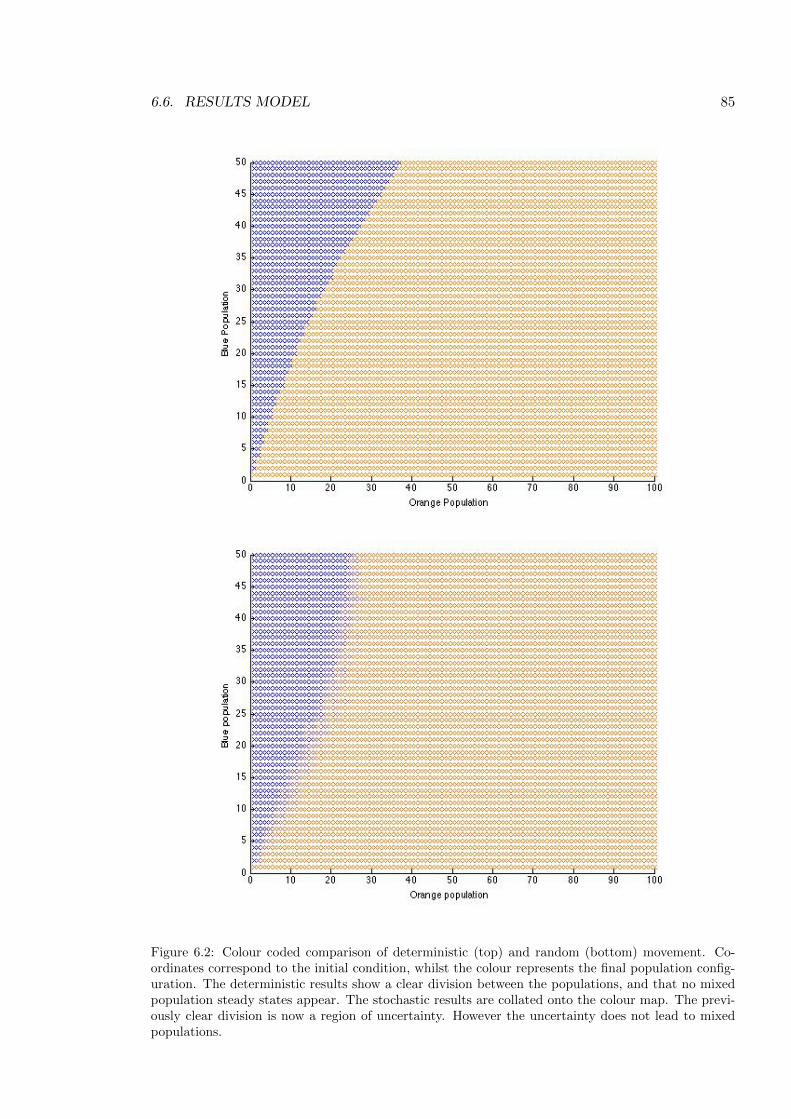
6.6. RESULTS MODEL 85
Figure 6.2: Colour coded comparison of deterministic (top) and random (bottom) movement. Co-ordinates correspond to the initial condition, whilst the colour represents the final population config-uration. The deterministic results show a clear division between the populations, and that no mixedpopulation steady states appear. The stochastic results are collated onto the colour map. The previ-ously clear division is now a region of uncertainty. However the uncertainty does not lead to mixedpopulations.
86 CHAPTER 6. WHOSE MOVE IS IT ANYWAY?
Figure 6.3: The population flow of the random movement rule, plotted on a two dimensional plane(bottom). The stochastic nature of agent movement partially obscures the parabolas that are clearlyshown in the deterministic model (top).
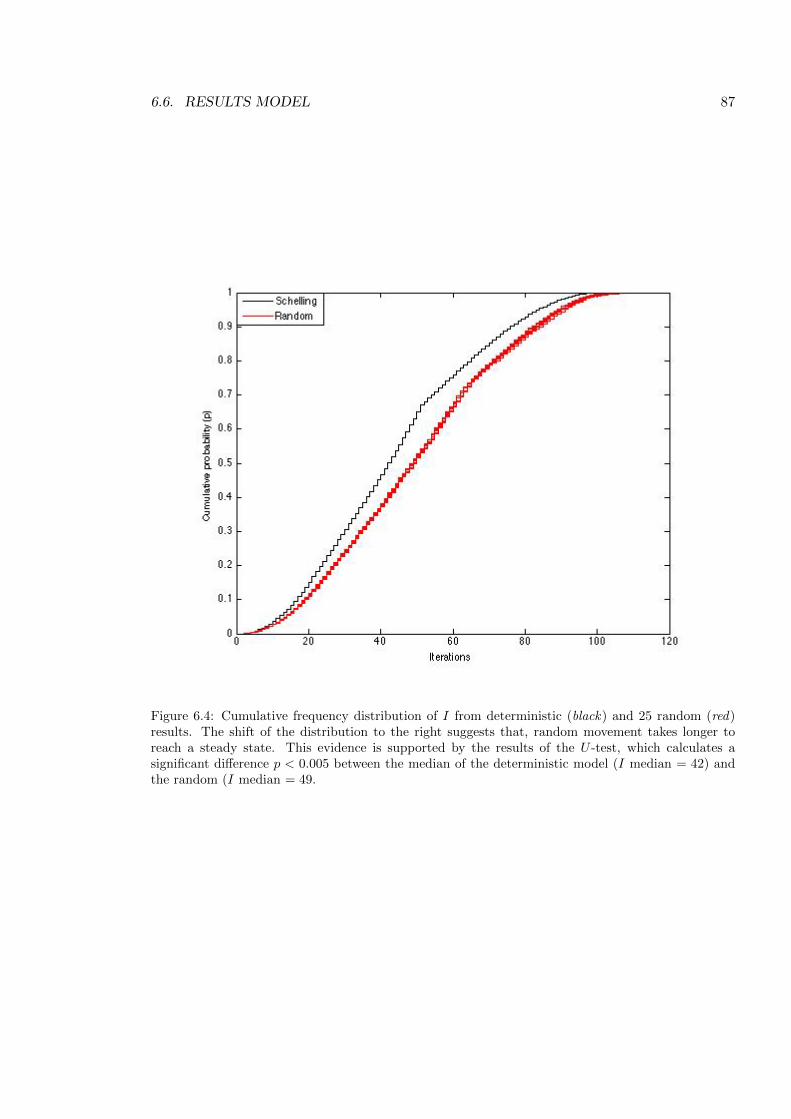
6.6. RESULTS MODEL 87
Figure 6.4: Cumulative frequency distribution of I from deterministic (black) and 25 random (red)results. The shift of the distribution to the right suggests that, random movement takes longer toreach a steady state. This evidence is supported by the results of the U -test, which calculates asignificant di↵erence p < 0.005 between the median of the deterministic model (I median = 42) andthe random (I median = 49.
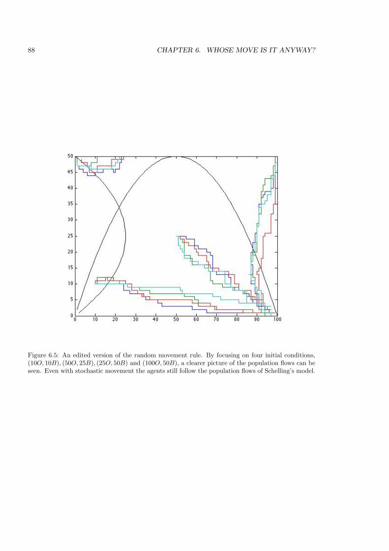
88 CHAPTER 6. WHOSE MOVE IS IT ANYWAY?
Figure 6.5: An edited version of the random movement rule. By focusing on four initial conditions,(10O, 10B), (50O, 25B), (25O, 50B) and (100O, 50B), a clearer picture of the population flows can beseen. Even with stochastic movement the agents still follow the population flows of Schelling’s model.
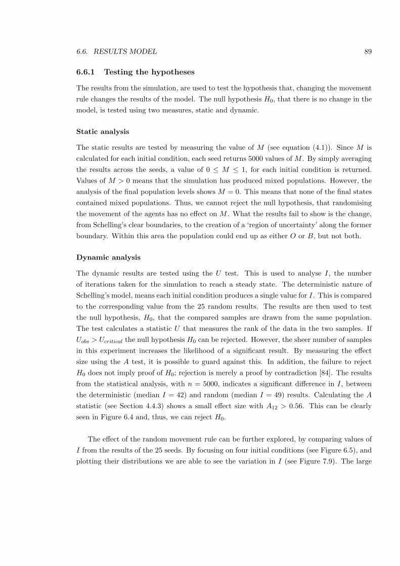
6.6. RESULTS MODEL 89
6.6.1 Testing the hypotheses
The results from the simulation, are used to test the hypothesis that, changing the movement
rule changes the results of the model. The null hypothesis H0, that there is no change in the
model, is tested using two measures, static and dynamic.
Static analysis
The static results are tested by measuring the value of M (see equation (4.1)). Since M is
calculated for each initial condition, each seed returns 5000 values of M . By simply averaging
the results across the seeds, a value of 0 M 1, for each initial condition is returned.
Values of M > 0 means that the simulation has produced mixed populations. However, the
analysis of the final population levels shows M = 0. This means that none of the final states
contained mixed populations. Thus, we cannot reject the null hypothesis, that randomising
the movement of the agents has no e↵ect on M . What the results fail to show is the change,
from Schelling’s clear boundaries, to the creation of a ‘region of uncertainty’ along the former
boundary. Within this area the population could end up as either O or B, but not both.
Dynamic analysis
The dynamic results are tested using the U test. This is used to analyse I, the number
of iterations taken for the simulation to reach a steady state. The deterministic nature of
Schelling’s model, means each initial condition produces a single value for I. This is compared
to the corresponding value from the 25 random results. The results are then used to test
the null hypothesis, H0, that the compared samples are drawn from the same population.
The test calculates a statistic U that measures the rank of the data in the two samples. If
Uobs > Ucritical the null hypothesis H0 can be rejected. However, the sheer number of samples
in this experiment increases the likelihood of a significant result. By measuring the e↵ect
size using the A test, it is possible to guard against this. In addition, the failure to reject
H0 does not imply proof of H0; rejection is merely a proof by contradiction [84]. The results
from the statistical analysis, with n = 5000, indicates a significant di↵erence in I, between
the deterministic (median I = 42) and random (median I = 49) results. Calculating the A
statistic (see Section 4.4.3) shows a small e↵ect size with A12 > 0.56. This can be clearly
seen in Figure 6.4 and, thus, we can reject H0.
The e↵ect of the random movement rule can be further explored, by comparing values of
I from the results of the 25 seeds. By focusing on four initial conditions (see Figure 6.5), and
plotting their distributions we are able to see the variation in I (see Figure 7.9). The large
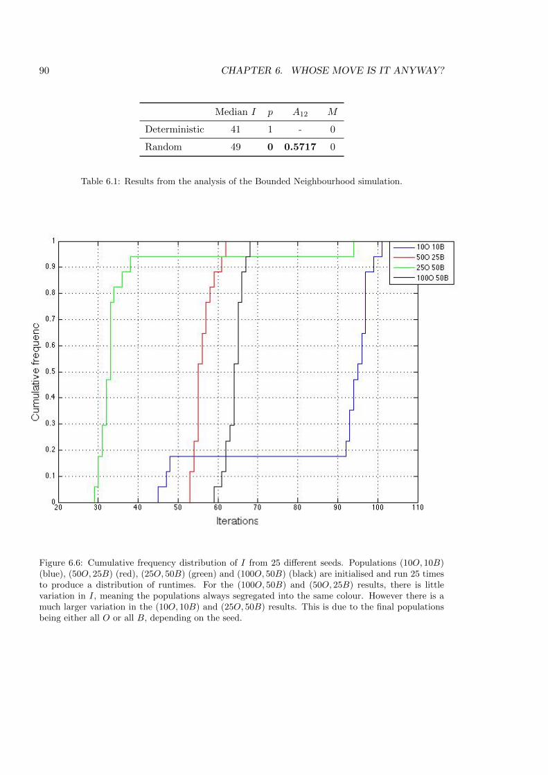
90 CHAPTER 6. WHOSE MOVE IS IT ANYWAY?
Median I p A12 M
Deterministic 41 1 - 0
Random 49 0 0.5717 0
Table 6.1: Results from the analysis of the Bounded Neighbourhood simulation.
Figure 6.6: Cumulative frequency distribution of I from 25 di↵erent seeds. Populations (10O, 10B)(blue), (50O, 25B) (red), (25O, 50B) (green) and (100O, 50B) (black) are initialised and run 25 timesto produce a distribution of runtimes. For the (100O, 50B) and (50O, 25B) results, there is littlevariation in I, meaning the populations always segregated into the same colour. However there is amuch larger variation in the (10O, 10B) and (25O, 50B) results. This is due to the final populationsbeing either all O or all B, depending on the seed.
6.7. CONCLUSIONS 91
variation in the distributions, for the initial conditions (10O, 10B) and (25O, 50B), can be
attributed to the di↵erence in the number of iterations taken to reach one of the two final
states. Since there are less iterations to reach 50B, compared to 100O, initial conditions
that reach both have a wider distribution. Since the random movement of an individual in a
smaller populations has more of an e↵ect, this result is unsurprising for the initial population
(10O, 10B). What is more interesting is the final population configuration, this is O around
80% of the time, as opposed to the expected 66%1. More surprising is the initial population
(25O, 50B). This population initialises at the maximum ⌧ for the O population and, as
such, should segregate to B. However the results indicate that, around 5% of the time the
population segregates to O. Both these results highlight the increased dominance of the O
population. However, when compared to results from the original simulation, none of the
results returned a significant di↵erence (see Table 6.2).
6.7 Conclusions
The work presented here, explored the e↵ect of Schelling’s deterministic movement rule. The
results show that changing the the movement rule in the Bounded Neighbourhood Model,
from ordered to random movement, causes a significant di↵erence in the number of itera-
tions (I) taken to reach stability. By applying the Vargha-Delaney test, we have shown the
di↵erence is not just a consequence of the number of samples used in analysis. However,
the changes have no e↵ect on the final population configuration of the model, as the only
stable populations are totally segregated (M = 0). The ability to a↵ect, what Schelling
would call, “the process of occupation” [74, 170] but not the final segregation, highlights the
model’s resistance to change. In addition the change in the movement rules increased the
dominance of the Orange population. In the original model, there was a definite divide of
RBO = 2 : 1 for B < 25. Any population initialising above that ratio would end up Blue,
those below ended up Orange. However, the ratio steadily decreases as B increases, meaning
when B = 50, RBO = 1.5 : 1. In the random model, the divide becomes blurred and changes
shape, so that, RBO ⇡ 2 : 1 8B. This is because it is no longer the most unhappy moving
(which, when RBO > 1, is an Orange), instead one is chosen at random. This means that,
when B > 25 and RBO ⇡ 2 : 1, although a Blue is more likely to be ‘happy’, they are twice
as likely to be chosen.
The distribution of the Schelling model shows a disjoint in the curve. The distribution
suggests that, by the time 50 iterations have been reached the model has reached a steady
1which is expected because the O population is twice that of B. This means the population would beexpected to dominate, from an equal initial condition, two-thirds of the time (or 66%).
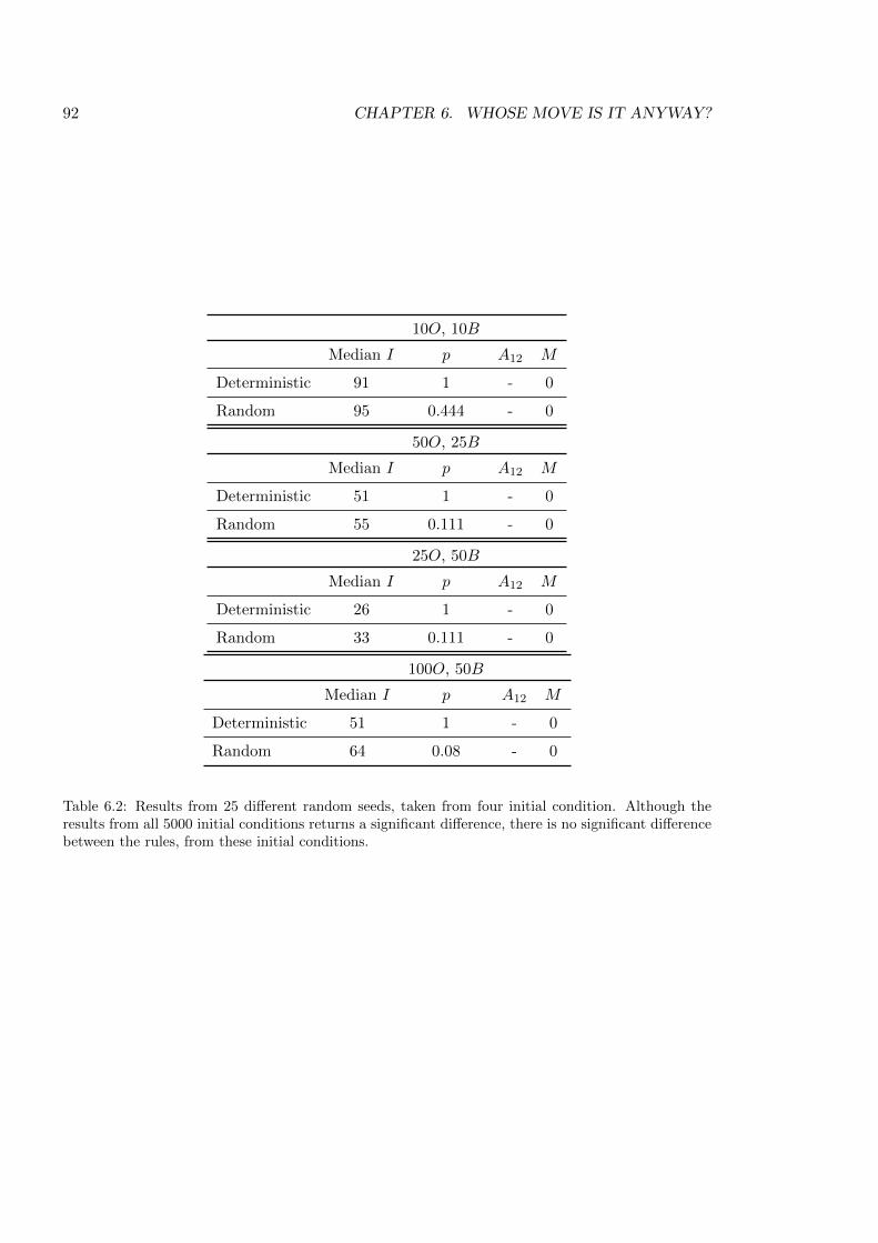
92 CHAPTER 6. WHOSE MOVE IS IT ANYWAY?
10O, 10B
Median I p A12 M
Deterministic 91 1 - 0
Random 95 0.444 - 0
50O, 25B
Median I p A12 M
Deterministic 51 1 - 0
Random 55 0.111 - 0
25O, 50B
Median I p A12 M
Deterministic 26 1 - 0
Random 33 0.111 - 0
100O, 50B
Median I p A12 M
Deterministic 51 1 - 0
Random 64 0.08 - 0
Table 6.2: Results from 25 di↵erent random seeds, taken from four initial condition. Although theresults from all 5000 initial conditions returns a significant di↵erence, there is no significant di↵erencebetween the rules, from these initial conditions.
6.7. CONCLUSIONS 93
state 66% of the time. This is due to the disparity in population sizes, since by 50 iterations
the entire B population will have made their moves, but only half of the O. This means
that, although the majority population dominate the final mix, the minority population
reach their steady state more quickly. This can be seen when exploring the results from
di↵erent seeds from certain initial conditions. Here the distributions of I, for certain initial
conditions, were stretched by the final configurations being either all O or all B. Further
examination suggests that randomising the movement of the agents, increases the dominance
of the majority population. However, no significant di↵erence was found in the runtimes
from the four selected initial conditions. This suggests that the significant di↵erence in the
original results was an artefact of the sample size. However, the results of the distributions
(Figure 7.9) show a similar increase compared to the cumulative results in Figure 6.4. This
means none of the random results reach stability before the expected result. Whilst this is
not completely unsurprising, it highlights the simplicity of the model. Since, with a more
complex model, one could expect a random results to perform at least as well at least once,
compared to the control. The overall results suggest that, whilst the ordered movement of
agents quickens the process of segregation, there is no discernible e↵ect on the segregation
of the populations. This can be seen as altering the kinetics of physical processes, but not
the thermodynamics. It is clear that, a much more significant alteration to the movement of
agents is necessary to change the stability of the system. Simply randomising those who are
leaving is not enough to change the results of segregation the model, however the random
movement can change the colour of the final population.
Further work could explore increasing the uncertainty in the model, by choosing from all
the agents at random, rather than from those who wish to move.. Even so, the experiment has
shown that the segregation is not driven simply by the order of agent movement. Although
this might seem an obvious statement, it is important to be able to provide evidence for
it. In addition, this has been a successful application of the CoSMoS process to Schelling’s
model. Continuing the process, the results from the simulation are fed back into the Schelling
Segregation model, increasing understanding, and raising new questions.

94 CHAPTER 6. WHOSE MOVE IS IT ANYWAY?
Chapter 7
Who do you know?
“Information is perfect: everybody knows the color ratio within the area at the
moment he makes his choice.” [74, p168]
7.1 Introduction
In Schelling’s Bounded Neighbourhood Model, agents have a precise knowledge of the colour
ratio of the neighbourhood. From this knowledge they make a decision about moving. Pre-
vious work (Chapter 6) has shown that, although changing the order of movement increases
the number of iterations taken to reach a steady state, the final outcome is always complete
segregation. In this chapter, rather than calculating the ratio from the neighbourhood in its
entirety, agents select a sample of other agents in the neighbourhood, and use that to calculate
their ratio. This means that agents no longer have a uniform response to the environment.
7.2 Hypothesis
Consistent with Chapter 6, the null hypothesis (H0) is that changing the agents’ perception
will have no e↵ect on the results of the simulation. This is tested using the two familiar
measures, static and dynamic.
7.2.1 Static measure
The static measure M is used to analyse the mix of the final population. M is calculated
according to equation (4.1), and compared to the mix of M = 0, resulting from Schelling’s
model. Values of M > 0 indicate mixed populations and highlight a change in the results.
95
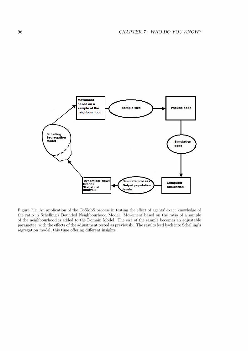
96 CHAPTER 7. WHO DO YOU KNOW?
Figure 7.1: An application of the CoSMoS process in testing the e↵ect of agents’ exact knowledge ofthe ratio in Schelling’s Bounded Neighbourhood Model. Movement based on the ratio of a sampleof the neighbourhood is added to the Domain Model. The size of the sample becomes an adjustableparameter, with the e↵ects of the adjustment tested as previously. The results feed back into Schelling’ssegregation model, this time o↵ering di↵erent insights.
7.3. DOMAIN MODEL 97
7.2.2 Dynamic measure
The dynamic measure tests whether the changes in the model, e↵ects the population flows.
This is tested by measuring the parameter I (described in Section 5.4), and comparing it to
the results from the original simulation. The results are analysed using the Mann-Whitney-
Wilcoxon U test and (if necessary) the Vargha-Delaney A statistic (described in Section 4.4.5).
7.3 Domain model: sampling the neighbourhood
The language of the Domain Model is retained from the formalisation presented in Chapter
5. Two populations of agents on 2 O and bn 2 B, calculate the ratio of the neighbourhood E
(RBO and ROB respectively). Agents compare R against their tolerance ⌧ . If the comparison
is unfavourable, on(⌧) < RBO or bn(⌧) < ROB the agent leaves the neighbourhood.
7.3.1 Changes to the Domain Model
In this extension agents take a random sample (S) of the neighbourhood (E) and use it to
calculate a sample ratio. This gives the ratio for on 2 O population as
RBOS =#(B \ S)
#(O \ S), (7.1)
with an equivalent equation for bn of
ROBS =#(O \ S)
#(B \ S). (7.2)
It is useful that, as S approaches E, the model tends to Schelling’s Bounded Neighbourhood
Model, since this can be used to validate the simulation.
7.4 Platform Model
The implementation of the alteration to the model is shown in algorithms 10 and 11. The
algorithms show the process for an agent on, an equivalent process governs the bn agents. The
only change to the algorithms presented in Section 5.2 is the calculation of R in algorithm 8.
Creating a sample ratio from the total neighbourhood is a simple change in how the variables
used to calculate the ratio are ascertained. Now agents take a random sample (S) of the
neighbourhood and use it to calculate a sample ratio ROBS or RBOS . This new ratio calcu-
lation propagates through the Platform Model, changing ROB and RBO to ROBS and RBOS
98 CHAPTER 7. WHO DO YOU KNOW?
Algorithm 10 Agent type o ‘happiness’ calculation: one timestep
calculate sample ratio RBOS
while on(⌧) < RBOS dofor each agent o 2 O do
if on(⌧) < RBOS thenset on [happy]
elseset on[unhappy]
end ifend forexecute Algorithm 11
end while
Algorithm 11 Agent type w movement rule: one timestep
if 9on 2 (O \ E⇤) with on(⌧) � RBOS thenmove on with max ⌧ to E
elseif 9on 2 (O \ E) with on(⌧) < RBOS then
set on with min ⌧ to E⇤
end ifend if
respectively. However, in other respects, the movement rule is unchanged from Schelling’s
original model, meaning agent’s still move in order of tolerance (see algorithm 11).
7.5 Simulation Platform
The Platform Model is simulated using Netlogo (see Section 5.2). Using this tool maintains
a consistency that is important for valid comparisons of results. In addition, Netlogo has
a number of useful environments that help facilitate the experiment. For example, the Be-
haviourSpace environment automates the testing of a number of di↵erent parameters, over
a range of values. This is useful for testing across all initial conditions, with varying values
of S. For consistency, the initial population values are retained from previous experiments.
This gives 5000 data points for each value of S. These are analysed to test the hypotheses
using the techniques set out previously (see Section 4.4). The values of the sample size S
are 150 (for validation) 75, 50, 25 and 10. These values, whilst arbitrary in some aspects,
nonetheless, o↵er a good sample representation of a range of possible sample sizes. Since
each sample is chosen randomly, 25 di↵erent runs of each initial condition are performed,
identical to Section 6.5.
7.6. RESULTS MODEL 99
7.6 Results Model
The results from the simulation are validated and analysed, using the static and dynamic
measures. The results of which provide evidence towards accepting, or refuting, H0.
7.6.1 Validation
The simulation is validated by setting S = 150 (the total number of agents). This makes
the sample the complete neighbourhood. As with the previous validation (Section 5.4.1)
the output is measured against Schelling’s results. The analysis of the static results shows
M = 0, whilst the colour maps are identical (Figure 7.2). The population flows are compared
in Figure 7.3 and show identical dynamics.
Following the validation of the simulation the remaining values of S are analysed. The
results are analysed using the static and dynamic measures. This allows testing of H0, that
the reduction of agents’ knowledge has no e↵ect on the model. For the analysis of the static
results, M is calculated from the steady state, reached by each initial condition. The value
of M is then compared to Schelling’s findings of M = 0. The final populations from each
of those initial conditions, are displayed as colour maps (Figures 7.4 and 7.5). The dynamic
measure (I) is used to test for changes in the number of iterations the system takes to reach
a steady state. To give a visual comparison to Schelling’s work, the results are displayed as
flows (Figures 7.3, 7.6 and 7.7). The dynamic results are tested using the U test (described
in Section 4.4.3).
7.6.2 Static analysis
To test H0, a comparison of the final population configurations is made. Results can be seen
in Figures 7.4 and 7.5, as well as in Table 7.1. Final populations are represented by their
colour, with their location on the grid representing the initial condition. As can be seen, as
S is reduced the dominance of the O population is increased.
7.6.3 Dynamic analysis
The dynamic test of the hypothesis argues that changing S will have no e↵ect on I. The
population flows in Figures 7.6 and 7.7 show that, as the sample size is reduced, the flows of
the populations are disrupted (see Figures 7.5 and 7.5).
A comparison of the number of iterations (I) to reach a steady state is shown in Figure 7.8,
with a full analysis of results presented in table 7.1.
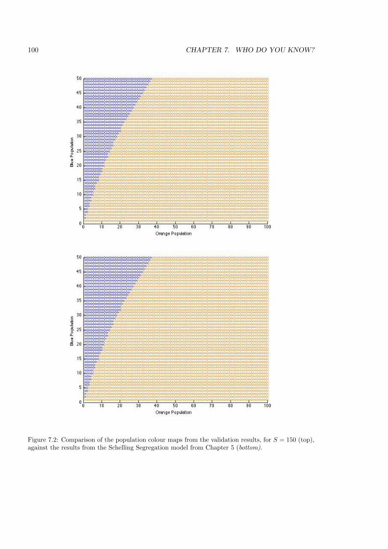
100 CHAPTER 7. WHO DO YOU KNOW?
Figure 7.2: Comparison of the population colour maps from the validation results, for S = 150 (top),against the results from the Schelling Segregation model from Chapter 5 (bottom).
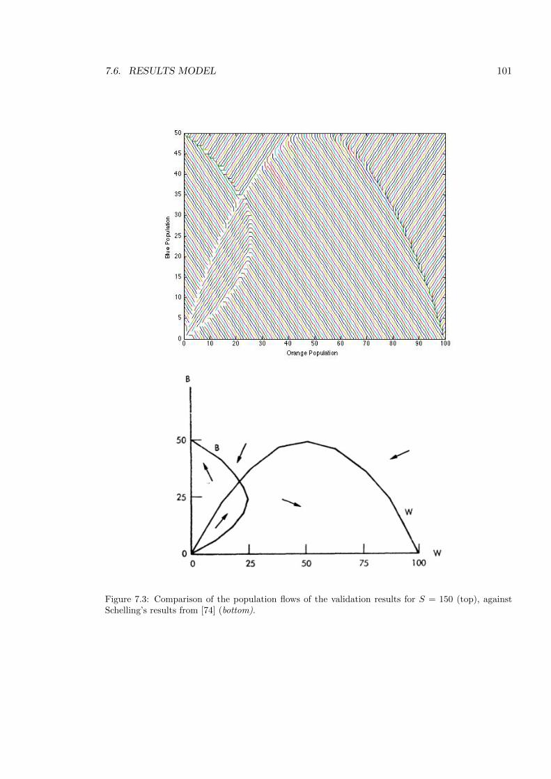
7.6. RESULTS MODEL 101
Figure 7.3: Comparison of the population flows of the validation results for S = 150 (top), againstSchelling’s results from [74] (bottom).
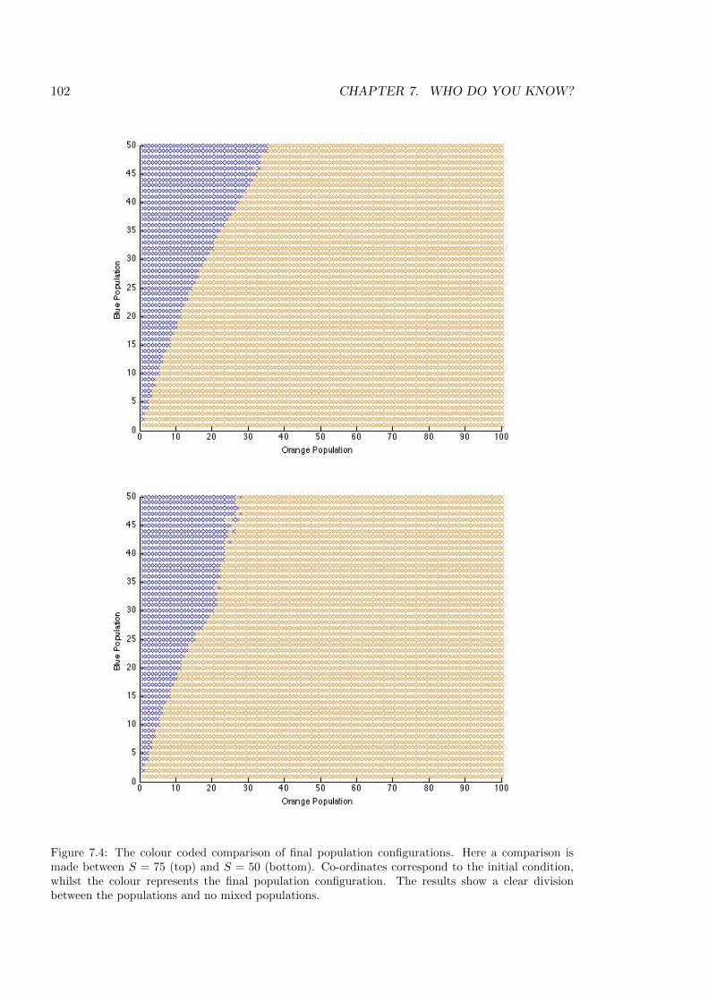
102 CHAPTER 7. WHO DO YOU KNOW?
Figure 7.4: The colour coded comparison of final population configurations. Here a comparison ismade between S = 75 (top) and S = 50 (bottom). Co-ordinates correspond to the initial condition,whilst the colour represents the final population configuration. The results show a clear divisionbetween the populations and no mixed populations.
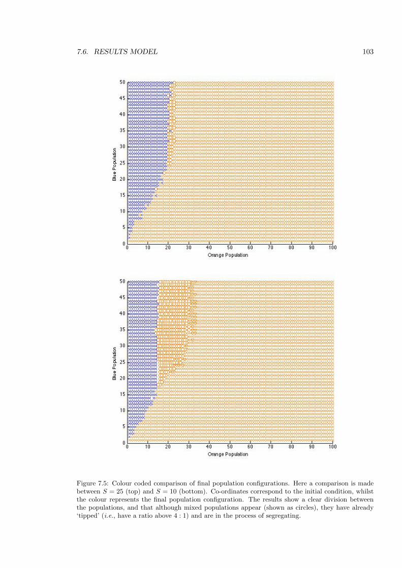
7.6. RESULTS MODEL 103
Figure 7.5: Colour coded comparison of final population configurations. Here a comparison is madebetween S = 25 (top) and S = 10 (bottom). Co-ordinates correspond to the initial condition, whilstthe colour represents the final population configuration. The results show a clear division betweenthe populations, and that although mixed populations appear (shown as circles), they have already‘tipped’ (i.e., have a ratio above 4 : 1) and are in the process of segregating.
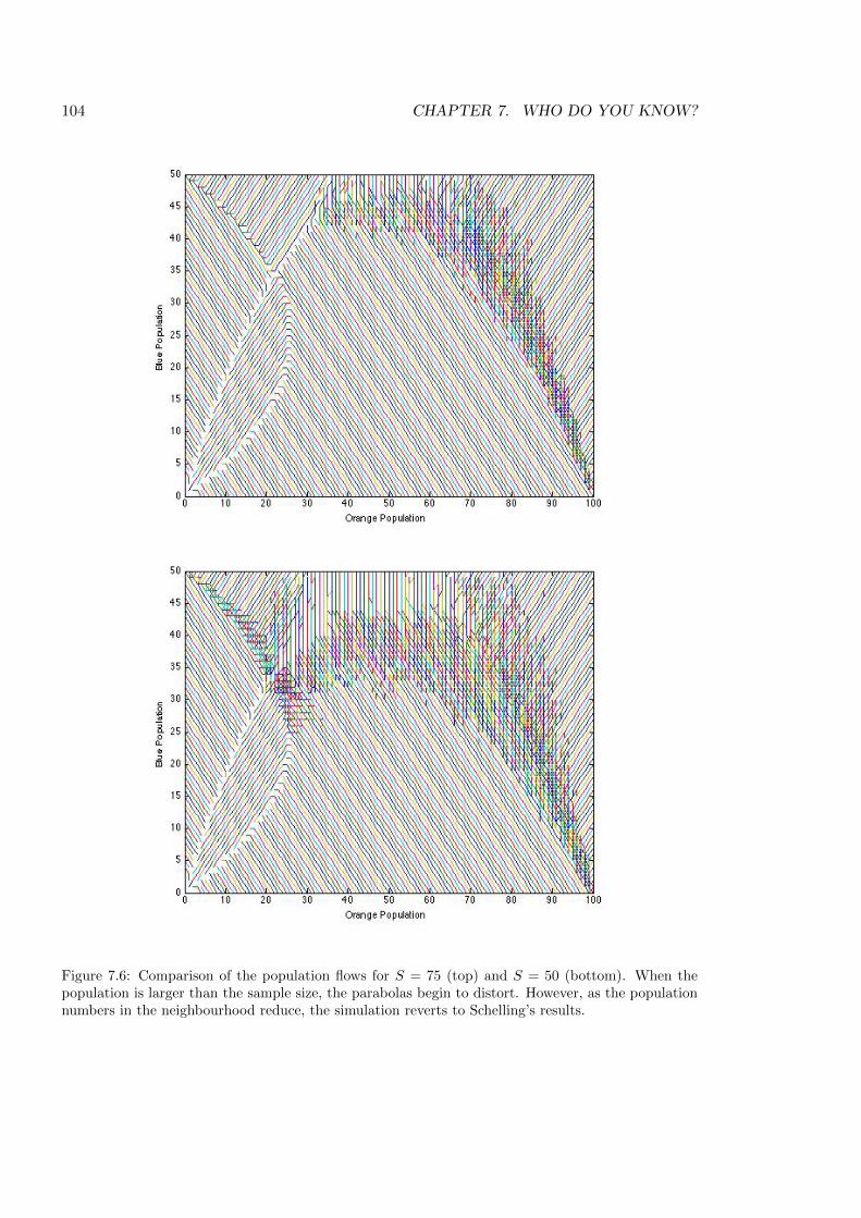
104 CHAPTER 7. WHO DO YOU KNOW?
Figure 7.6: Comparison of the population flows for S = 75 (top) and S = 50 (bottom). When thepopulation is larger than the sample size, the parabolas begin to distort. However, as the populationnumbers in the neighbourhood reduce, the simulation reverts to Schelling’s results.
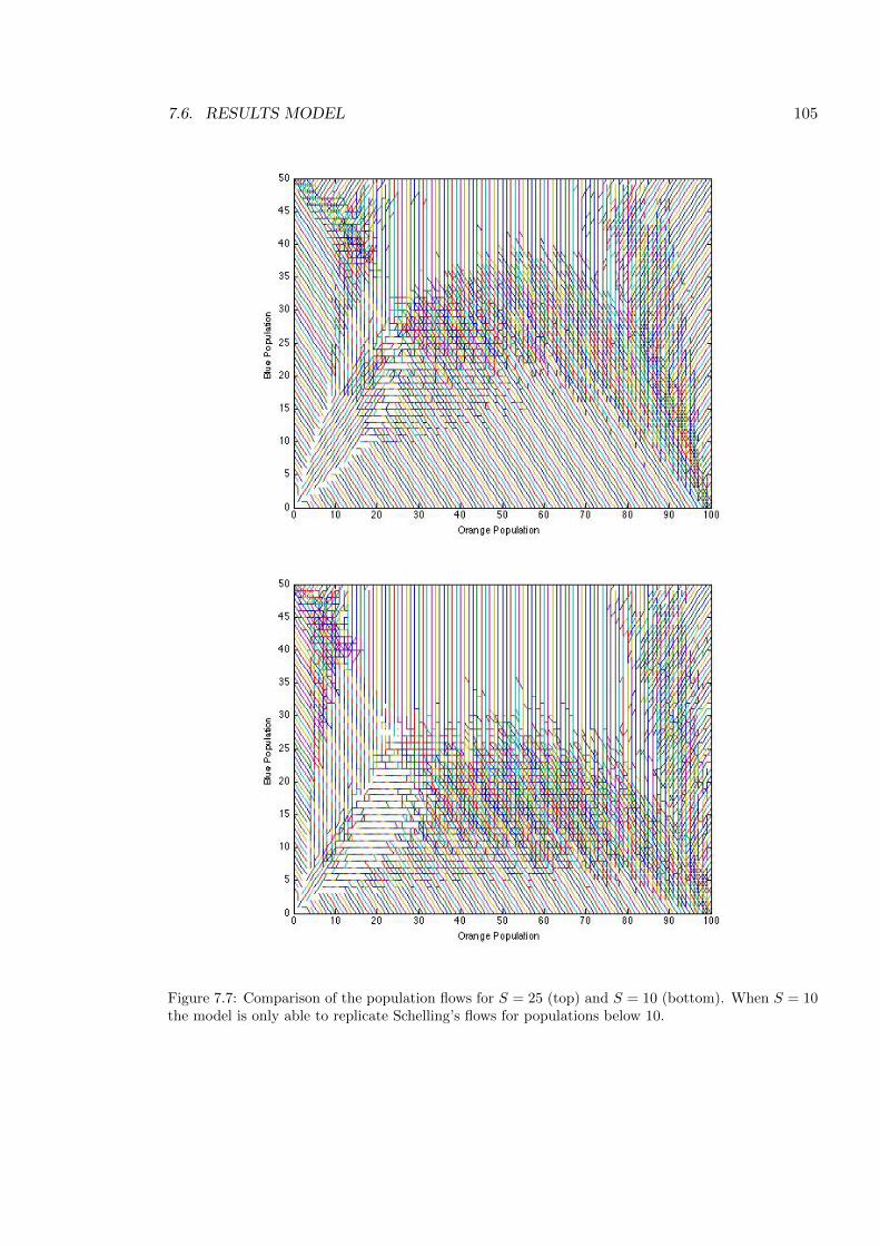
7.6. RESULTS MODEL 105
Figure 7.7: Comparison of the population flows for S = 25 (top) and S = 10 (bottom). When S = 10the model is only able to replicate Schelling’s flows for populations below 10.
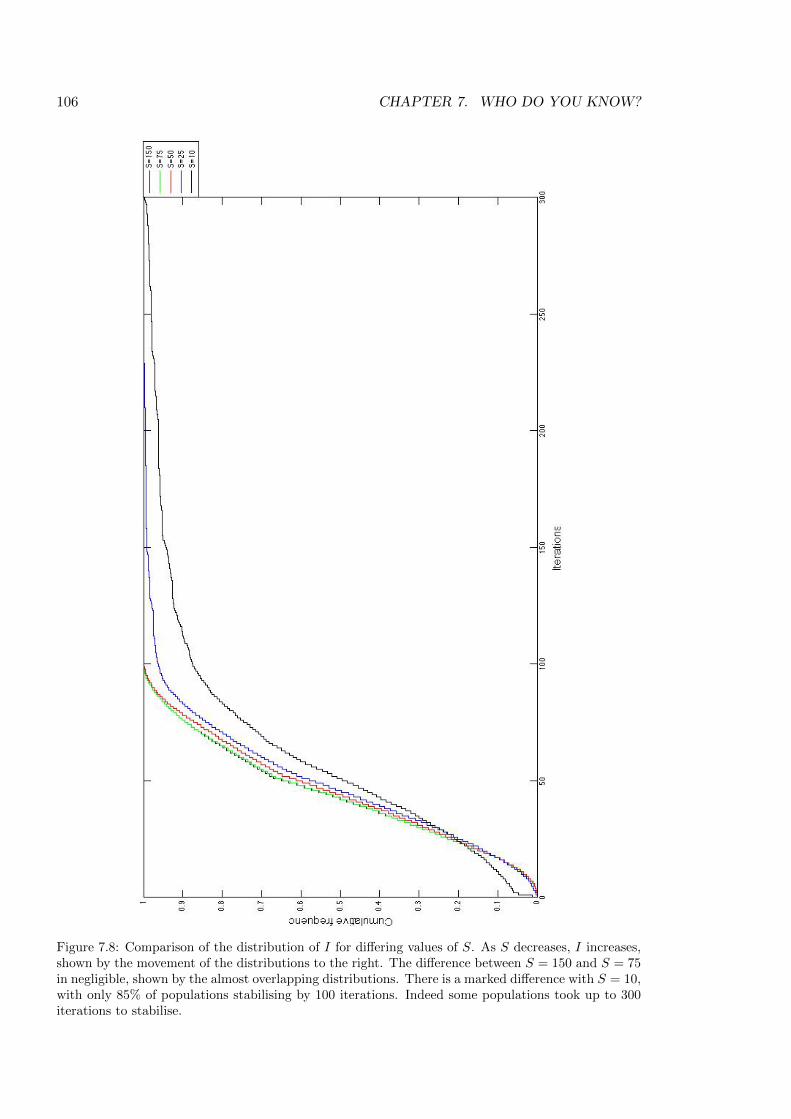
106 CHAPTER 7. WHO DO YOU KNOW?
Figure 7.8: Comparison of the distribution of I for di↵ering values of S. As S decreases, I increases,shown by the movement of the distributions to the right. The di↵erence between S = 150 and S = 75in negligible, shown by the almost overlapping distributions. There is a marked di↵erence with S = 10,with only 85% of populations stabilising by 100 iterations. Indeed some populations took up to 300iterations to stabilise.
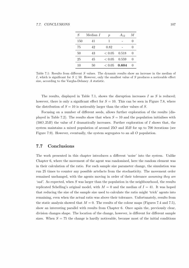
7.7. CONCLUSIONS 107
S Median I p A12 M
150 41 1 - 0
75 42 0.82 - 0
50 43 < 0.05 0.518 0
25 45 < 0.05 0.559 0
10 50 < 0.05 0.604 0
Table 7.1: Results from di↵erent S values. The dynamic results show an increase in the median ofI, which is significant for S 50. However, only the smallest value of S produces a noticeable e↵ectsize, according to the Vargha-Delaney A statistic.
The results, displayed in Table 7.1, shows the disruption increases I as S is reduced;
however, there is only a significant e↵ect for S = 10. This can be seen in Figure 7.8, where
the distribution of S = 10 is noticeably larger than the other values of S.
Focusing on a number of di↵erent seeds, allows further exploration of the results (dis-
played in Table 7.2). The results show that when S = 10 and the population initialises with
(50O, 25B) the value of I dramatically increases. Further exploration of I shows that, the
system maintains a mixed population of around 25O and 35B for up to 700 iterations (see
Figure 7.9). However, eventually, the system segregates to an all O population.
7.7 Conclusions
The work presented in this chapter introduces a di↵erent ‘noise’ into the system. Unlike
Chapter 6, where the movement of the agent was randomised, here the random element was
in their calculation of the ratio. For each sample size parameter change, the simulation was
run 25 times to counter any possible artefacts from the stochasticity. The movement order
remained unchanged, with the agents moving in order of their tolerance assuming they are
‘sad’. As expected, when S was larger than the population in the neighbourhood, the results
replicated Schelling’s original model, with M = 0 and the median of I = 41. It was hoped
that reducing the size of the sample size used to calculate the ratio might ‘trick’ agents into
remaining, even when the actual ratio was above their tolerance. Unfortunately, results from
the static analysis showed that M = 0. The results of the colour maps (Figures 7.4 and 7.5),
show an interesting parallel with results from Chapter 6. Once again the, previously clear,
division changes shape. The location of the change, however, is di↵erent for di↵erent sample
sizes. When S = 75 the change is hardly noticeable, because most of the initial conditions
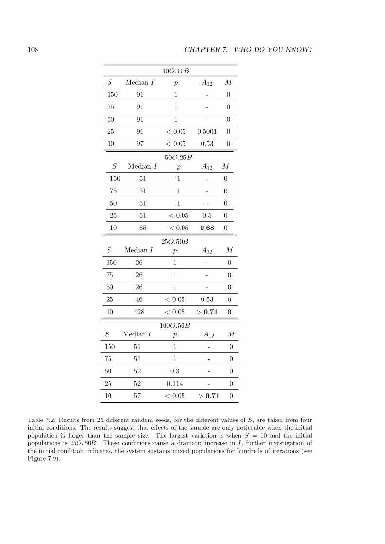
108 CHAPTER 7. WHO DO YOU KNOW?
10O,10B
S Median I p A12 M
150 91 1 - 0
75 91 1 - 0
50 91 1 - 0
25 91 < 0.05 0.5001 0
10 97 < 0.05 0.53 0
50O,25BS Median I p A12 M
150 51 1 - 0
75 51 1 - 0
50 51 1 - 0
25 51 < 0.05 0.5 0
10 65 < 0.05 0.68 0
25O,50BS Median I p A12 M
150 26 1 - 0
75 26 1 - 0
50 26 1 - 0
25 46 < 0.05 0.53 0
10 428 < 0.05 > 0.71 0
100O,50BS Median I p A12 M
150 51 1 - 0
75 51 1 - 0
50 52 0.3 - 0
25 52 0.114 - 0
10 57 < 0.05 > 0.71 0
Table 7.2: Results from 25 di↵erent random seeds, for the di↵erent values of S, are taken from fourinitial conditions. The results suggest that e↵ects of the sample are only noticeable when the initialpopulation is larger than the sample size. The largest variation is when S = 10 and the initialpopulations is 25O, 50B. These conditions cause a dramatic increase in I, further investigation ofthe initial condition indicates, the system sustains mixed populations for hundreds of iterations (seeFigure 7.9).
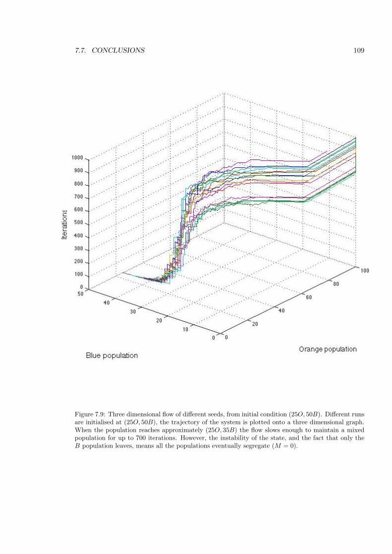
7.7. CONCLUSIONS 109
Figure 7.9: Three dimensional flow of di↵erent seeds, from initial condition (25O, 50B). Di↵erent runsare initialised at (25O, 50B), the trajectory of the system is plotted onto a three dimensional graph.When the population reaches approximately (25O, 35B) the flow slows enough to maintain a mixedpopulation for up to 700 iterations. However, the instability of the state, and the fact that only theB population leaves, means all the populations eventually segregate (M = 0).
110 CHAPTER 7. WHO DO YOU KNOW?
a↵ected have populations less than the sample size (i.e., they revert to the Schelling model).
By S = 50 the change is noticeable for initial conditions with a population above 50. When
S = 25 the results are most similar to the random movement change, with the divide blurring
along RBO ⇡ 2 : 1. By S = 10, whilst the divide is broadly the same shape, the region of
uncertainty has increased. The dynamic result provided evidence that reducing S increased
I, with a significant increase (median of I = 50) when S = 10. Further exploration has
shown the increase is due to the system sustaining mixed populations for hundreds of it-
erations (see Figure 7.9). Whilst, this is a promising result, only the B population would
only leave. Once they had left, they would not return and the O population begins to dom-
inate the neighbourhood. These results o↵er evidence that H0 can be rejected. Although
mixed populations arose, and were briefly maintained, the populations would all eventually
segregate. The results from the experiment show that reducing the knowledge of the agents
increases the number of iterations taken to reach a steady state. Indeed, for S = 10 unsta-
ble mixed populations appeared; however, eventually, all the populations segregated. This
highlights the precariousness of mixed populations, compared to the segregated populations.
Once segregated the sampling has no e↵ect, since no matter what the sample will always be
the same. When the population is mixed the ratio of the sample can change, displacing the
balance. This is something that could be explored further as, it would appear, the system
is beginning to sustain mixed populations. It is possible that the slowing of the population
dynamics, could be a route towards increasing the stability of mixed populations. If agents
were prevented from leaving the moment ⌧ < R, it is possible that the flow of other agents
could alter R enough such that ⌧ � R.

Chapter 8
Should I stay, or should I go?
“If a person’s limit is exceeded in this area he will go someplace else–a place, pre-
sumably, where his own color predominates or where color does not matter..” [74,
p167]
8.1 Introduction
In Schelling’s model, the moment an agent can no longer tolerate the ratio of the neigh-
bourhood, they leave. Previous results (Section 6.6) have shown that, although changing
the order of movement can slow the population dynamics, the model is unable to produce
anything other than complete segregation. In the Bounded Neighbourhood Model, agents in
the population move as soon as they are ‘sad’, to any place that is more tolerable. However,
movement should have a cost. If agent movement was restricted, the system might change
enough for the agent to remain.
In this modification, we define a ‘sadness’ parameter. Now, the movement of the agents is
based on a probability derived from their level of ‘sadness’ relative to the second neighbour-
hood. Agents attempt to minimise their ‘sadness’ by switching to the other neighbourhood.
By considering the problem in terms of energy minimisation, a friction parameter F is defined
to indirectly ‘control’ the flow of the system. These characteristics are added to the Domain
model in Section 8.3, and from there (following the CoSMoS process) the Platform Model
is adjusted. The Simulaton Platform is used to run the model and produce results that are
used to test the hypothesis described below.
111
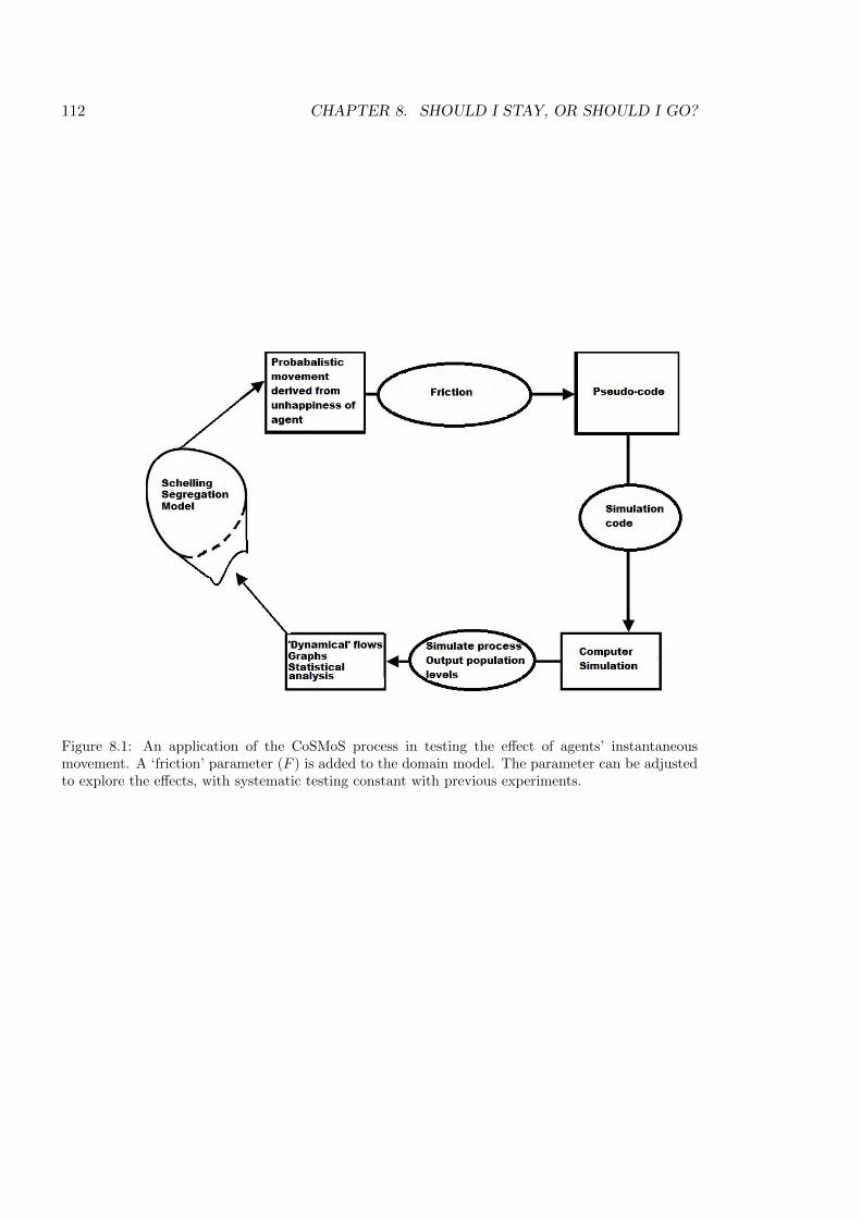
112 CHAPTER 8. SHOULD I STAY, OR SHOULD I GO?
Figure 8.1: An application of the CoSMoS process in testing the e↵ect of agents’ instantaneousmovement. A ‘friction’ parameter (F ) is added to the domain model. The parameter can be adjustedto explore the e↵ects, with systematic testing constant with previous experiments.
8.2. HYPOTHESIS 113
8.2 Hypothesis
The null hypothesis (H0) argues that, increasing F will have no e↵ect on the results of the
model. The static and dynamic measures (M and I) are used in the analysis of results, and
testing of the hypothesis.
8.2.1 Static measure
The static measure analyses the final population configurations. Using Equation (4.1) the
mix of the population M is measured and compared to the results from Schelling’s model,
where M = 0. Values of M > 0 indicates mixed populations have arisen.
8.2.2 Dynamic measure
The dynamic measure analyses the flows of the populations into and out of the neighbourhood.
The U test (described in Section 4.4.3 is used to analyse the results of the number I of
iterations, testing the e↵ects of the changes of the model. Results that return significant
results undergo further analysis using the A statistic (described in Section 4.4.5).
8.3 Domain model: adding friction
The parameters and language of the Domain Model are retained (see Section 5.1). The
‘sadness’ of an agent (on 2 O)1 is calculated thus
on(u) = RBO � on(⌧) (8.1)
where on(⌧) is the tolerance of the agent on and RBO is the ratio inside the neighbourhood (see
(5.3)). However, problems arise with agents who find themselves ‘‘outside” the neighbourhood
(on 2 (O \ E⇤)), but are calculating their ‘sadness’ based on the ratio inside (RBO, see
equation (5.5)). Agents that are inside (on 2 (O \ E)) now have di↵erent behaviours from
those outside (i.e., if an agent is ‘sad’ inside they move but if they are ‘sad’ outside they stay
outside).
8.3.1 Changes to the model
In the extension considered in this chapter, agents now utilise the ratio of a second neigh-
bourhood E⇤. Introduced in Section 5.1, E⇤ was simply (in Schelling’s words) “someplace
1As with the previous Domain Model the agent on 2 O has an equivalent agent bn 2 B.
114 CHAPTER 8. SHOULD I STAY, OR SHOULD I GO?
else” [74, p168]. In this extension, E⇤ is defined as the neighbourhood where the agent is
considering moving to. Thus, the ratio of E⇤ is needed to allow a comparison and (for the O
population) is given by the ratio
RBO⇤ =(B \ E⇤)
(O \ E⇤). (8.2)
The agents on use this ratio in the equation
on(u⇤) = RBO⇤
� on(⌧), (8.3)
to calculate their ‘sadness’ if they switch neighbourhoods. By comparing this value with u,
the ‘sadness’ di↵erence �u is calculated,
�u = u� u⇤. (8.4)
The same equations are used to calculate the �u of the B population. It is reasonable to
assume that smaller �u is, the more likely an agent will move. This can be modelled as
follows. Substitute �u for x into the exponential function e�x and dividing the exponent
��u by a friction parameter (F ) to obtain a function e��u/F that decreases steeply to 0 as
�u decreases and increases up to 1 as F increases. The movement of agents, can be modelled
by a probability derived from �u and ‘controlled’ by F :
P (stay) = min{1, e��u/F}. (8.5)
This means that, as �u increases, the probability of staying decreases; as F increases the
probability of staying increases (Figure 8.2). Thus, instead of agents moving as soon as they
are sad, their movement is controlled by a probability, based on the di↵erence between the
ratio of populations. If �u < 0, agents will not move, since it implies that R⇤ > R, where R
and R⇤ are the respective neighbourhood ratios.
8.4 Platform Model
Using the structure and language developed in Section 5.2, the Platform Model is presented
using algorithms 12 and 13. Agent movement is based on the calculation of P [stay], shown
in the movement calculation algorithm 13. Now the question remains as to the order of
movement. In Schelling’s model, agents moved “in order of their tolerance” [74, p167],
if agents are moving into, and out of, two neighbourhoods, both of which are now being
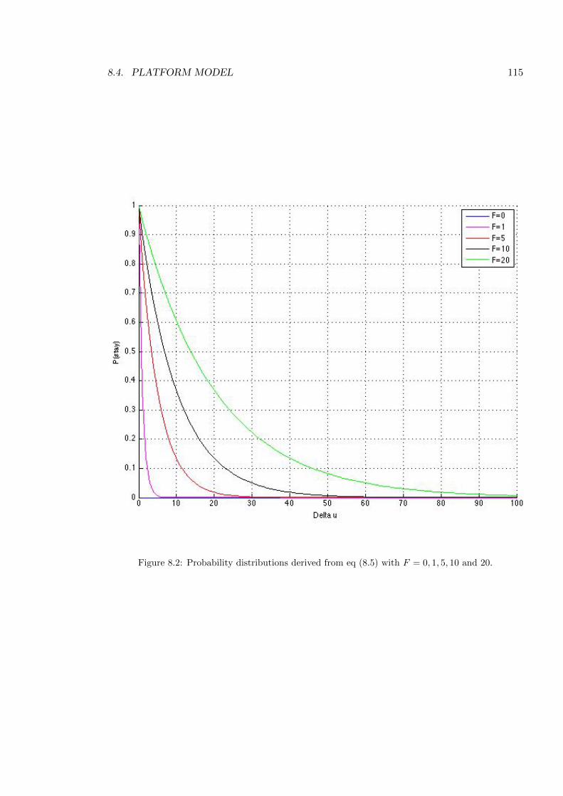
8.4. PLATFORM MODEL 115
Figure 8.2: Probability distributions derived from eq (8.5) with F = 0, 1, 5, 10 and 20.
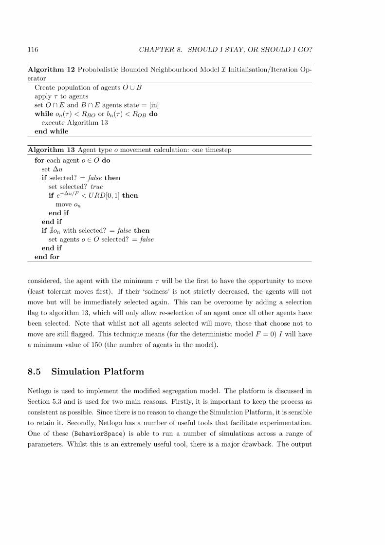
116 CHAPTER 8. SHOULD I STAY, OR SHOULD I GO?
Algorithm 12 Probabalistic Bounded Neighbourhood Model I Initialisation/Iteration Op-eratorCreate population of agents O [Bapply ⌧ to agentsset O \ E and B \ E agents state = [in]while on(⌧) < RBO or bn(⌧) < ROB doexecute Algorithm 13
end while
Algorithm 13 Agent type o movement calculation: one timestep
for each agent o 2 O doset �uif selected? = false then
set selected? trueif e��u/F < URD[0, 1] thenmove on
end ifend ifif @on with selected? = false then
set agents o 2 O selected? = falseend if
end for
considered, the agent with the minimum ⌧ will be the first to have the opportunity to move
(least tolerant moves first). If their ‘sadness’ is not strictly decreased, the agents will not
move but will be immediately selected again. This can be overcome by adding a selection
flag to algorithm 13, which will only allow re-selection of an agent once all other agents have
been selected. Note that whilst not all agents selected will move, those that choose not to
move are still flagged. This technique means (for the deterministic model F = 0) I will have
a minimum value of 150 (the number of agents in the model).
8.5 Simulation Platform
Netlogo is used to implement the modified segregation model. The platform is discussed in
Section 5.3 and is used for two main reasons. Firstly, it is important to keep the process as
consistent as possible. Since there is no reason to change the Simulation Platform, it is sensible
to retain it. Secondly, Netlogo has a number of useful tools that facilitate experimentation.
One of these (BehaviorSpace) is able to run a number of simulations across a range of
parameters. Whilst this is an extremely useful tool, there is a major drawback. The output
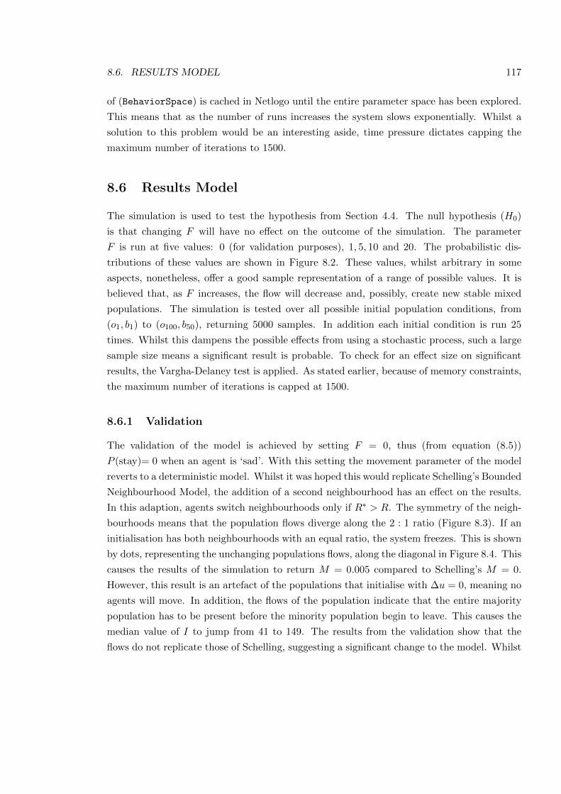
8.6. RESULTS MODEL 117
of (BehaviorSpace) is cached in Netlogo until the entire parameter space has been explored.
This means that as the number of runs increases the system slows exponentially. Whilst a
solution to this problem would be an interesting aside, time pressure dictates capping the
maximum number of iterations to 1500.
8.6 Results Model
The simulation is used to test the hypothesis from Section 4.4. The null hypothesis (H0)
is that changing F will have no e↵ect on the outcome of the simulation. The parameter
F is run at five values: 0 (for validation purposes), 1, 5, 10 and 20. The probabilistic dis-
tributions of these values are shown in Figure 8.2. These values, whilst arbitrary in some
aspects, nonetheless, o↵er a good sample representation of a range of possible values. It is
believed that, as F increases, the flow will decrease and, possibly, create new stable mixed
populations. The simulation is tested over all possible initial population conditions, from
(o1, b1) to (o100, b50), returning 5000 samples. In addition each initial condition is run 25
times. Whilst this dampens the possible e↵ects from using a stochastic process, such a large
sample size means a significant result is probable. To check for an e↵ect size on significant
results, the Vargha-Delaney test is applied. As stated earlier, because of memory constraints,
the maximum number of iterations is capped at 1500.
8.6.1 Validation
The validation of the model is achieved by setting F = 0, thus (from equation (8.5))
P (stay)= 0 when an agent is ‘sad’. With this setting the movement parameter of the model
reverts to a deterministic model. Whilst it was hoped this would replicate Schelling’s Bounded
Neighbourhood Model, the addition of a second neighbourhood has an e↵ect on the results.
In this adaption, agents switch neighbourhoods only if R⇤ > R. The symmetry of the neigh-
bourhoods means that the population flows diverge along the 2 : 1 ratio (Figure 8.3). If an
initialisation has both neighbourhoods with an equal ratio, the system freezes. This is shown
by dots, representing the unchanging populations flows, along the diagonal in Figure 8.4. This
causes the results of the simulation to return M = 0.005 compared to Schelling’s M = 0.
However, this result is an artefact of the populations that initialise with �u = 0, meaning no
agents will move. In addition, the flows of the population indicate that the entire majority
population has to be present before the minority population begin to leave. This causes the
median value of I to jump from 41 to 149. The results from the validation show that the
flows do not replicate those of Schelling, suggesting a significant change to the model. Whilst
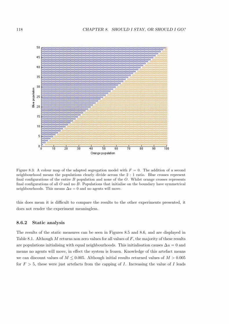
118 CHAPTER 8. SHOULD I STAY, OR SHOULD I GO?
Figure 8.3: A colour map of the adapted segregation model with F = 0. The addition of a secondneighbourhood means the populations clearly divide across the 2 : 1 ratio. Blue crosses representfinal configurations of the entire B population and none of the O. Whilst orange crosses representsfinal configurations of all O and no B. Populations that initialise on the boundary have symmetricalneighbourhoods. This means �u = 0 and no agents will move.
this does mean it is di�cult to compare the results to the other experiments presented, it
does not render the experiment meaningless.
8.6.2 Static analysis
The results of the static measures can be seen in Figures 8.5 and 8.6, and are displayed in
Table 8.1. AlthoughM returns non zero values for all values of F , the majority of these results
are populations initialising with equal neighbourhoods. This initialisation causes �u = 0 and
means no agents will move, in e↵ect the system is frozen. Knowledge of this artefact means
we can discount values of M 0.005. Although initial results returned values of M > 0.005
for F > 5, these were just artefacts from the capping of I. Increasing the value of I leads
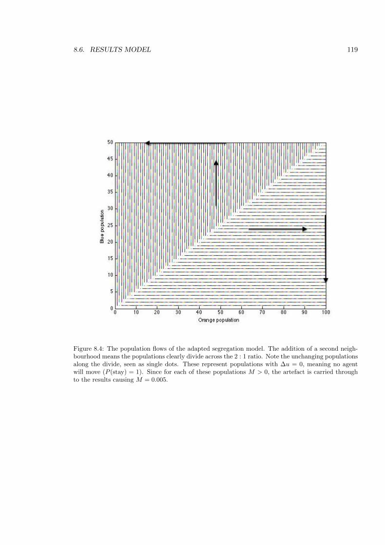
8.6. RESULTS MODEL 119
Figure 8.4: The population flows of the adapted segregation model. The addition of a second neigh-bourhood means the populations clearly divide across the 2 : 1 ratio. Note the unchanging populationsalong the divide, seen as single dots. These represent populations with �u = 0, meaning no agentwill move (P (stay) = 1). Since for each of these populations M > 0, the artefact is carried throughto the results causing M = 0.005.
120 CHAPTER 8. SHOULD I STAY, OR SHOULD I GO?
F Median I p A12 M
0 149 1 - 0.005
1 220 0 > 0.71 0.005
5 588 0 > 0.71 0.005
10 1088 0 > 0.71 0.005
20 2214 0 > 0.71 0.005
Table 8.1: Results from di↵erent F values. The dynamic results show a significant result, with a largee↵ect size for even the smallest value of F . Although the results for M indicate mixed populationsthey are actually artefacts of the simulation. The M value is a result of the populations that initialisedwith perfectly balanced neighbourhoods (i.e., �u = 0), meaning no agents will move.
to M = 0.005 (see Table 8.1). As figures 8.7 and 8.8 show, the populations are still clearly
segregated along the 2 : 1 boundary.
8.6.3 Dynamic analysis
The results from the dynamic analysis are displayd in Figures 8.7 and 8.8. They show that as
F increases, the flow of the population is disrupted (i.e., the number of iterations I increases).
This can be seen in a comparison of the population runtimes shown in Figure 8.9. When
F = 0 the median I = 149, setting F = 1 increases the median I = 220. This increase
is due to the system having to iterate through the population twice more, before reaching
stability. This can be seen by the plateaus in the distributions every 150 iterations. As F
increases further, increase between plateaus is reduced, suggesting less systems stabilising
at each round of iterations. It is noticeable that when F > 5 the maximum I is reached
before the system reaches stability. Although for F = 5 this only happens in 5% of cases,
for F = 10 it has increased to 35% and, by F = 20 around 66% of populations have failed
to reach stability. This artefact means the median I for F = 20 is 1500. By increasing the
maximum I the results for F = 20 return a median I = 2214. However, adjusting F had no
e↵ect on populations initialised with identical neighbourhoods. This is because of �u = 0
so, no matter the value of F , P (stay) = 1.
8.7 Conclusions
The work presented in this chapter has explored the e↵ect of restricting agent movement.
This has been tested by introducing a parameter F to control the ease of movement in the
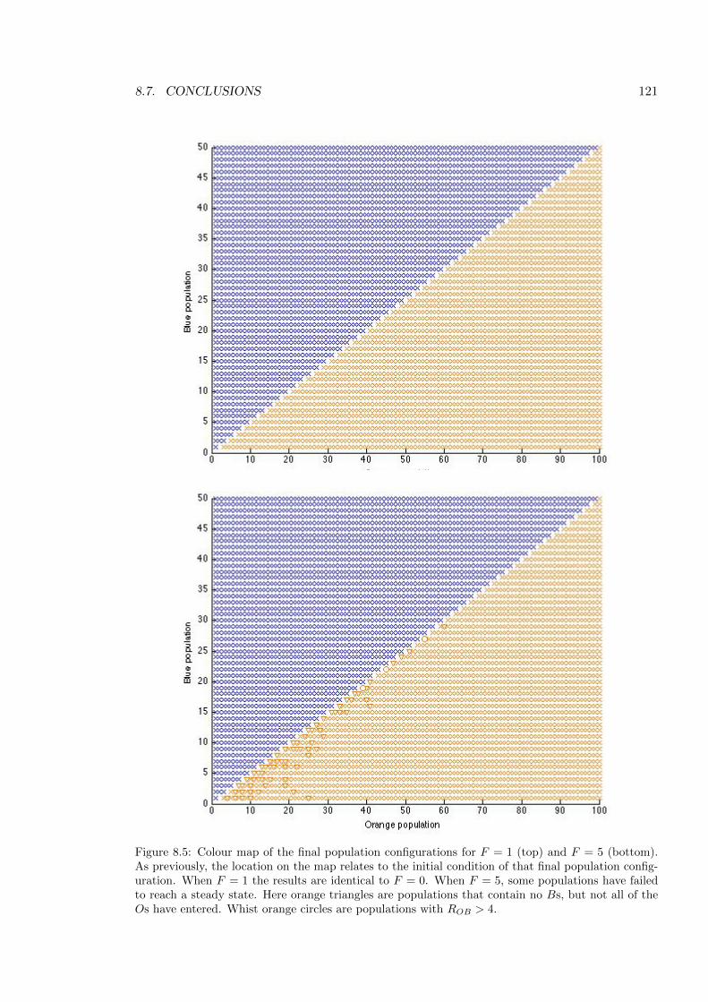
8.7. CONCLUSIONS 121
Figure 8.5: Colour map of the final population configurations for F = 1 (top) and F = 5 (bottom).As previously, the location on the map relates to the initial condition of that final population config-uration. When F = 1 the results are identical to F = 0. When F = 5, some populations have failedto reach a steady state. Here orange triangles are populations that contain no Bs, but not all of theOs have entered. Whist orange circles are populations with ROB > 4.
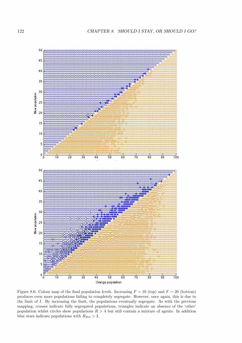
122 CHAPTER 8. SHOULD I STAY, OR SHOULD I GO?
Figure 8.6: Colour map of the final population levels. Increasing F = 10 (top) and F = 20 (bottom)produces even more populations failing to completely segregate. However, once again, this is due tothe limit of I. By increasing the limit, the populations eventually segregate. As with the previousmapping, crosses indicate fully segregated populations, triangles indicate an absence of the ‘other’population whilst circles show populations R > 4 but still contain a mixture of agents. In additionblue stars indicate populations with RBO > 3.
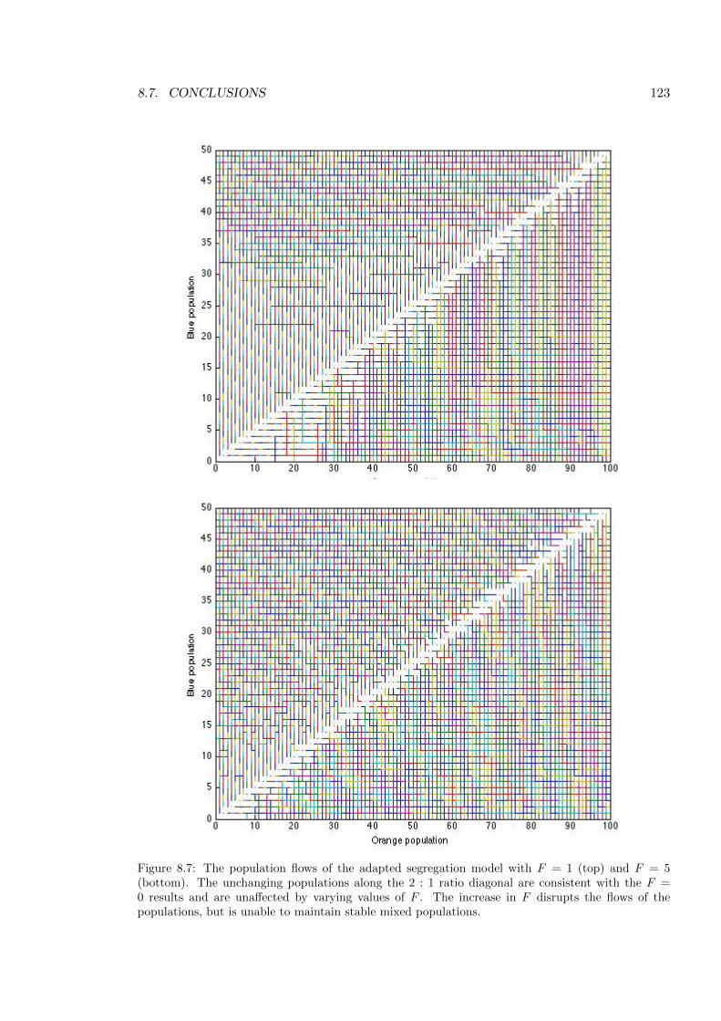
8.7. CONCLUSIONS 123
Figure 8.7: The population flows of the adapted segregation model with F = 1 (top) and F = 5(bottom). The unchanging populations along the 2 : 1 ratio diagonal are consistent with the F =0 results and are una↵ected by varying values of F . The increase in F disrupts the flows of thepopulations, but is unable to maintain stable mixed populations.
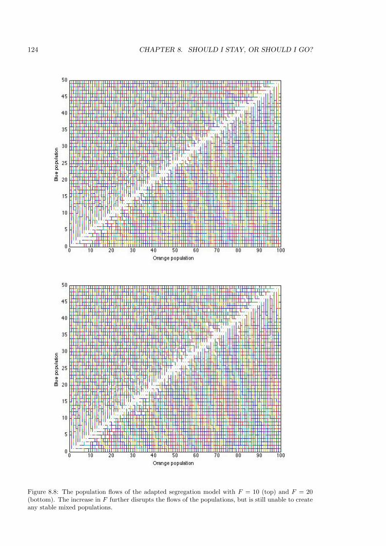
124 CHAPTER 8. SHOULD I STAY, OR SHOULD I GO?
Figure 8.8: The population flows of the adapted segregation model with F = 10 (top) and F = 20(bottom). The increase in F further disrupts the flows of the populations, but is still unable to createany stable mixed populations.
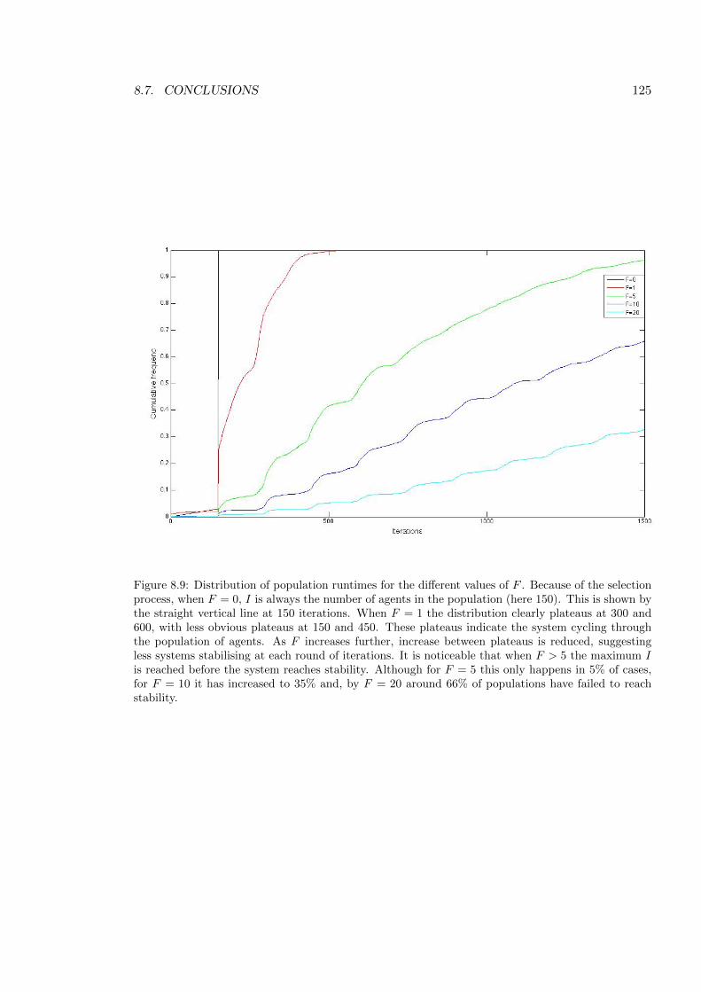
8.7. CONCLUSIONS 125
Figure 8.9: Distribution of population runtimes for the di↵erent values of F . Because of the selectionprocess, when F = 0, I is always the number of agents in the population (here 150). This is shown bythe straight vertical line at 150 iterations. When F = 1 the distribution clearly plateaus at 300 and600, with less obvious plateaus at 150 and 450. These plateaus indicate the system cycling throughthe population of agents. As F increases further, increase between plateaus is reduced, suggestingless systems stabilising at each round of iterations. It is noticeable that when F > 5 the maximum Iis reached before the system reaches stability. Although for F = 5 this only happens in 5% of cases,for F = 10 it has increased to 35% and, by F = 20 around 66% of populations have failed to reachstability.
126 CHAPTER 8. SHOULD I STAY, OR SHOULD I GO?
model. The adjustment has meant a second ‘comparison’ neighbourhood has been defined.
The validation of the model has provided evidence that the model produces di↵erent results
in both static and dynamic analysis. However the static results returning M > 0 have been
shown to be artefacts created from the calculation of �u. The failure of the validation means
the model cannot be considered a valid replication of Schelling’s Bounded Neighbourhood
Model. This makes the results di�cult to compare to either Schelling’s model, or the results
of other experiments. However, the results of the experiment are interesting, since they show
that even heavily restricting the movement of the agents is unable to prevent total segregation.
The experimentation on varying values of F , did initially suggest that the model maintained
mixed populations (M > 0). However, further analysis highlights two artefacts causing the
result. Firstly, when the system initialises with the two neighbourhoods having equal ratios,
no agents move. This is shown by the single dots, signifying unchanging populations, along
the diagonals of Figures 8.4, 8.7 and 8.8. The agents in these populations will not move,
because the identical ratio means �u = 0, leading to P (stay) = 1 and M = 0.005. Secondly,
as F is increased I also increases; however, since the maximum of I = 1500, the remaining
mixed populations are merely in the process of segregating. By increasing the maximum
value of I, the second artefact disappears. The results indicate that, the change in the model
produces a large e↵ect on the dynamic results but, even though stable mixed populations are
maintained, they are shown to be just an artefact of the model. The increase in I is a result
that is to be expected, since the adjustment to the model is the first time the movement of
the agents has been restricted. However, the failure of the validation test makes a comparison
between these results, and those from Chapters 6 and 7 di�cult. This means that, although
the change in the model shows a significant increase in I, it cannot be known if the results
are due to the change in the movement parameter, or the change in the environment. The
adjustment means that, although the model is able to replicate Schelling’s segregation, it is
unable to recreate Schelling’s flows. This reduces its defendability as a model of Schelling’s
Bounded Neighbourhood. However, the fact that a second neighbourhood can cause such an
e↵ect on the model is an important result. This suggests that the environment ‘outside’ the
model needs much more careful consideration before being applied, something that is often
disregarded in social interaction models.
Chapter 9
Friends and Neighbours
9.1 Introduction
Networks have been widely used to model social systems, such as group membership [42] and,
interestingly, segregation [38]. Networks are described in Section 2.4, so here we provide a
brief introduction to the additional concepts and terms needed for this chapter. Networks are
described in terms of nodes and their connections to other nodes. They are often characterised
in terms of distances between nodes (path length), connectivity (degree) and density ⇢. It is
natural to interpret nodes connected to a network being agents inside a neighbourhood, and
vice-versa. By describing Schelling’s Bounded Neighbourhood Model as a network, we can
exploit network techniques. As with the previous Bounded Neighbourhood Model, the ratio
of the neighbourhood network changes over the time of the run. As the ratio changes, nodes
(which, for consistency, we call agents) connect and disconnect from the neighbourhood,
until no more change their connection. Implementing a social network creates a subset of
agents in each of the population types. Those inside the social network alter the calculation
of the neighbourhood network. This allows the investigation of the e↵ect, if any, of the
di↵erentiation by type alone (i.e., there is no di↵erence between agents other than their
type).
9.2 Hypothesis
The hypotheses tests the e↵ects of recasting the model. We o↵er the null hypothesis (H0)
that recasting the model will have no e↵ect on the outcome of the simulation. This is tested
using two measures, static and dynamic (discussed in Section 4.4).
127
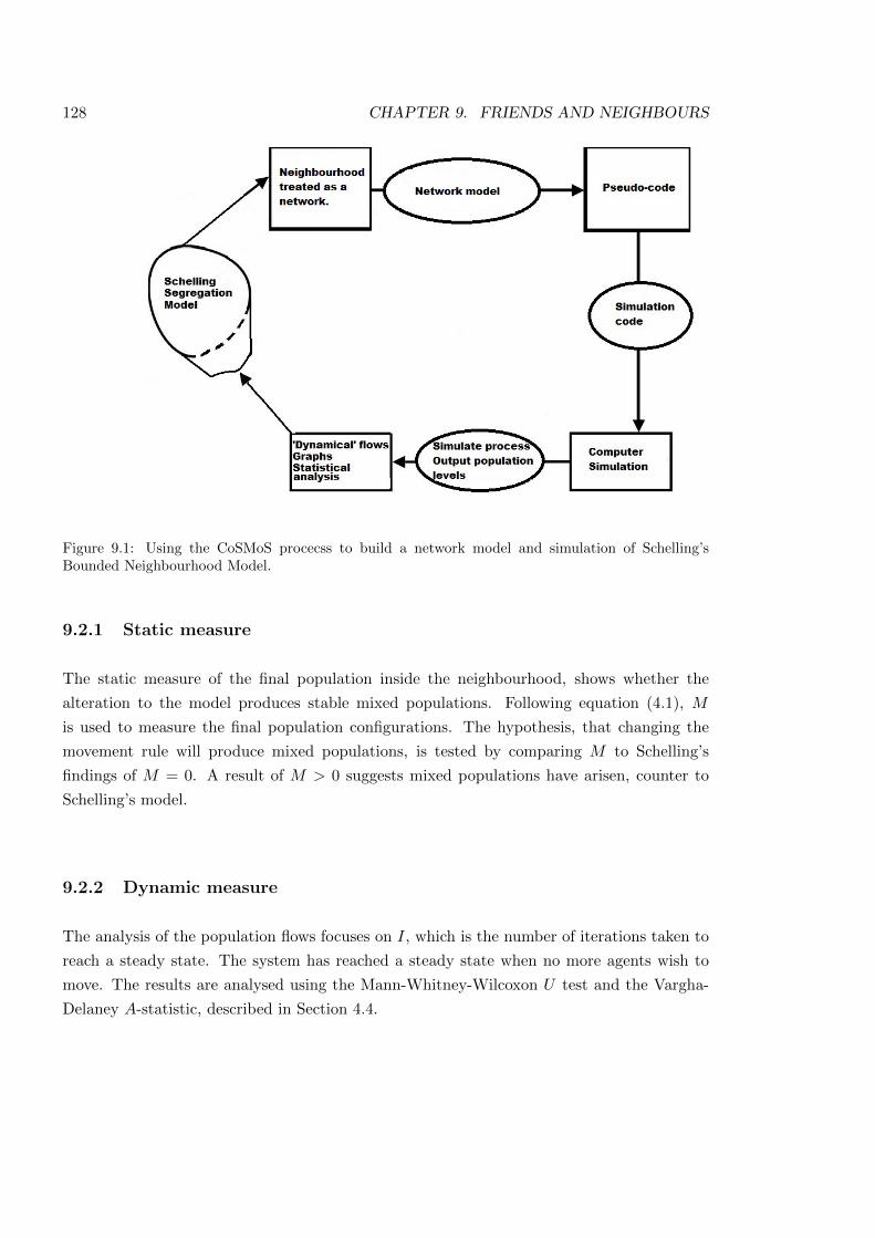
128 CHAPTER 9. FRIENDS AND NEIGHBOURS
Figure 9.1: Using the CoSMoS procecss to build a network model and simulation of Schelling’sBounded Neighbourhood Model.
9.2.1 Static measure
The static measure of the final population inside the neighbourhood, shows whether the
alteration to the model produces stable mixed populations. Following equation (4.1), M
is used to measure the final population configurations. The hypothesis, that changing the
movement rule will produce mixed populations, is tested by comparing M to Schelling’s
findings of M = 0. A result of M > 0 suggests mixed populations have arisen, counter to
Schelling’s model.
9.2.2 Dynamic measure
The analysis of the population flows focuses on I, which is the number of iterations taken to
reach a steady state. The system has reached a steady state when no more agents wish to
move. The results are analysed using the Mann-Whitney-Wilcoxon U test and the Vargha-
Delaney A-statistic, described in Section 4.4.
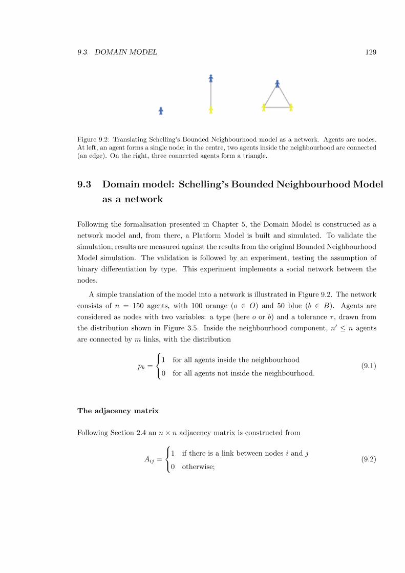
9.3. DOMAIN MODEL 129
Figure 9.2: Translating Schelling’s Bounded Neighbourhood model as a network. Agents are nodes.At left, an agent forms a single node; in the centre, two agents inside the neighbourhood are connected(an edge). On the right, three connected agents form a triangle.
9.3 Domain model: Schelling’s Bounded Neighbourhood Model
as a network
Following the formalisation presented in Chapter 5, the Domain Model is constructed as a
network model and, from there, a Platform Model is built and simulated. To validate the
simulation, results are measured against the results from the original Bounded Neighbourhood
Model simulation. The validation is followed by an experiment, testing the assumption of
binary di↵erentiation by type. This experiment implements a social network between the
nodes.
A simple translation of the model into a network is illustrated in Figure 9.2. The network
consists of n = 150 agents, with 100 orange (o 2 O) and 50 blue (b 2 B). Agents are
considered as nodes with two variables: a type (here o or b) and a tolerance ⌧ , drawn from
the distribution shown in Figure 3.5. Inside the neighbourhood component, n0 n agents
are connected by m links, with the distribution
pk =
8<
:1 for all agents inside the neighbourhood
0 for all agents not inside the neighbourhood.(9.1)
The adjacency matrix
Following Section 2.4 an n⇥ n adjacency matrix is constructed from
Aij =
8<
:1 if there is a link between nodes i and j
0 otherwise;(9.2)
130 CHAPTER 9. FRIENDS AND NEIGHBOURS
where i and j are i and jth agents in the network. This gives the matrix
A =
0
BBBBBBB@
0 A1,2 . . . A1,149 A1,150
A2,1 0 . . . A2,149 A2,150...
.... . .
......
A149,1 A149,2 . . . 0 A149,150
A150,1 A150,2 . . . A150,149 0
1
CCCCCCCA
(9.3)
Agents connected to the neighbourhood are defined as in E, and are fully connected to
all other agents in E. If |E| ⌘ n0, where |E| is the cardinality of E, then the number of
connections m can be calculated thus,
m =n0(n0
� 1)
2. (9.4)
The ratio for the O population, RBO, is derived from equation (5.3) giving:
RBO =n0(B)
n0(O). (9.5)
Similarly for the B population,
ROB =n0(O)
n0(B). (9.6)
Agents that are connected with ⌧ < R, disconnect from the network. They disconnect
from smallest to largest, in order of ⌧ and one at a time. When an agent disconnects from the
network (i.e., removes all links) they become completely disconnected, and become a node (or
component of one node). Amongst these components, if R changes enough such that R � ⌧ ,
the agent with largest ⌧ reconnects. Thus, the network is made up of one major component
(the neighbourhood), where all nodes are fully connected, whilst the rest are components of
single nodes. The number of components in the network can be calculated by (n � n0) + 1;
and can be used to verify the density of the network.1
9.4 Platform Model
The dynamics of the model are formalised in algorithms 14 and 15. The advantages of this
approach are discussed in Chapter 5. Briefly, the pseudo-code description is a useful stepping
stone from the model to the simulation. It gives an accurate representation of the model that
is easily translated into code.
1Since, as n0 ! n, the number of components ! 1.
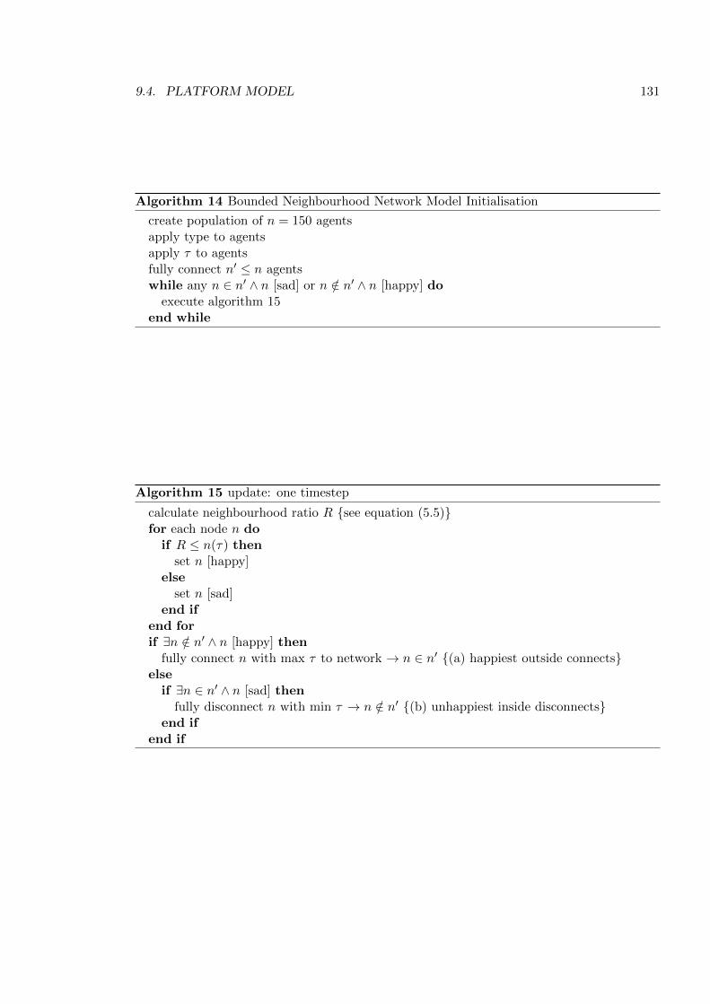
9.4. PLATFORM MODEL 131
Algorithm 14 Bounded Neighbourhood Network Model Initialisation
create population of n = 150 agentsapply type to agentsapply ⌧ to agentsfully connect n0
n agentswhile any n 2 n0
^ n [sad] or n /2 n0^ n [happy] do
execute algorithm 15end while
Algorithm 15 update: one timestep
calculate neighbourhood ratio R {see equation (5.5)}for each node n doif R n(⌧) then
set n [happy]else
set n [sad]end if
end forif 9n /2 n0
^ n [happy] thenfully connect n with max ⌧ to network ! n 2 n0
{(a) happiest outside connects}elseif 9n 2 n0
^ n [sad] thenfully disconnect n with min ⌧ ! n /2 n0
{(b) unhappiest inside disconnects}end if
end if
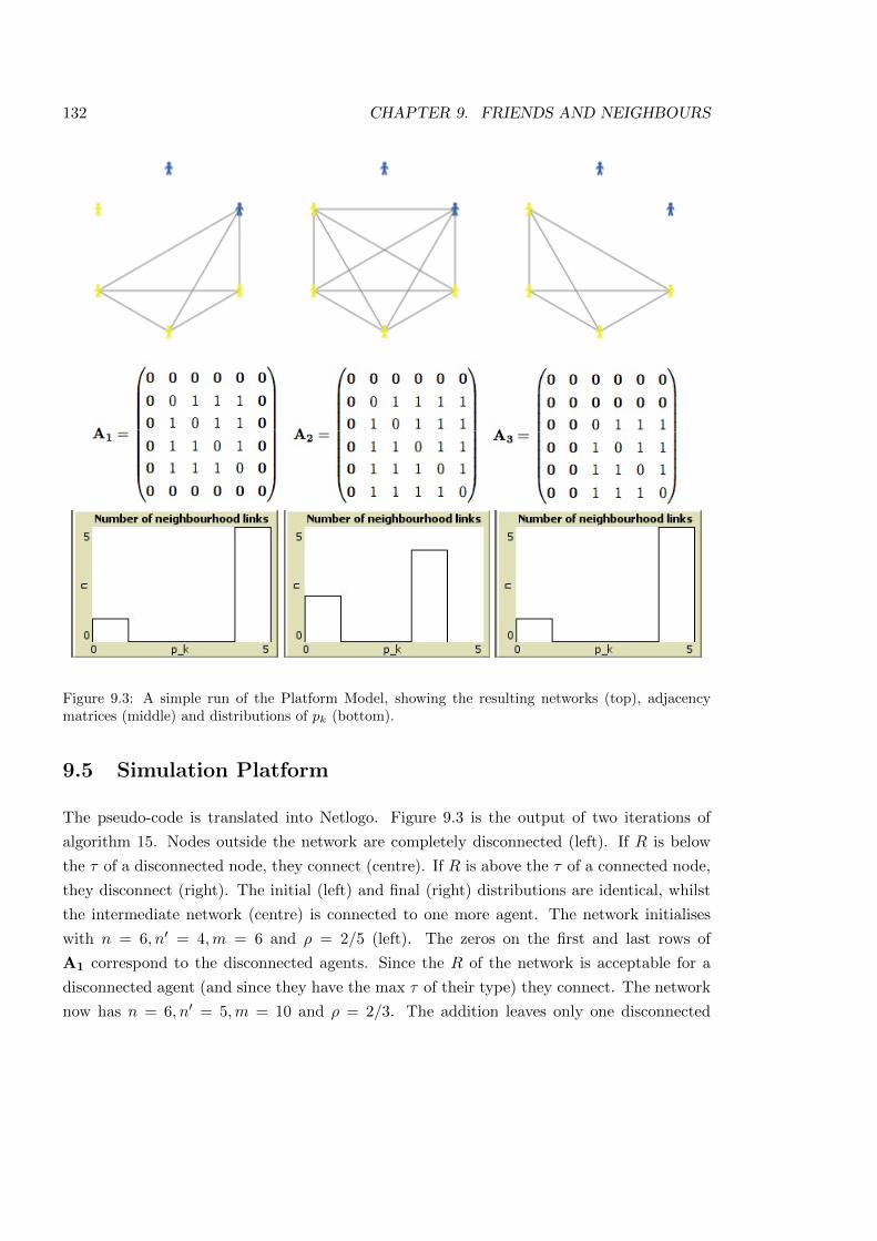
132 CHAPTER 9. FRIENDS AND NEIGHBOURS
Figure 9.3: A simple run of the Platform Model, showing the resulting networks (top), adjacencymatrices (middle) and distributions of pk (bottom).
9.5 Simulation Platform
The pseudo-code is translated into Netlogo. Figure 9.3 is the output of two iterations of
algorithm 15. Nodes outside the network are completely disconnected (left). If R is below
the ⌧ of a disconnected node, they connect (centre). If R is above the ⌧ of a connected node,
they disconnect (right). The initial (left) and final (right) distributions are identical, whilst
the intermediate network (centre) is connected to one more agent. The network initialises
with n = 6, n0 = 4,m = 6 and ⇢ = 2/5 (left). The zeros on the first and last rows of
A1 correspond to the disconnected agents. Since the R of the network is acceptable for a
disconnected agent (and since they have the max ⌧ of their type) they connect. The network
now has n = 6, n0 = 5,m = 10 and ⇢ = 2/3. The addition leaves only one disconnected
9.6. RESULTS MODEL 133
agent, highlighted in A2. In addition R has increased for the blue agents and decreased for
the orange. Since no ‘happy’ agents exist outside the network, the removal of ‘sad’ agents is
activated, leading to the final configuration (right). In this configuration, no agents change
their connection to the network, and the run is terminated. In this case the network has an
identical makeup to the first network with n = 6, n0 = 4,m = 6 and ⇢ = 2/5. However the
di↵erence betweenA1 andA3, highlights the di↵erent nodes connected to the neighbourhood.
9.6 Results Model
To check the validity of the model, the results of the simulation are measured against the
results from the original Schelling simulation (see Chapter 5). As with previous experiments,
the same initial conditions are used (see Chapter 6). In network terms, each possible adja-
cency matrix is constructed. This gives 5000 matrices, which are run until a steady state
is achieved. When the network reaches a steady state (defined as the point where no more
nodes wish to connect or disconnect), the number of iterations is recorded (I) and the pop-
ulation configuration is measured (M). Since the model is deterministic, there is only need
for a single run across all the initial conditions. As previously, due to memory constraints,
the maximum value of I is capped to 1500.
The simulation results of the population dynamics, are measured against the results from
the original Bounded Neighbourhood Model simulation (see Chapter 6). The comparison
of flows (shown in Figure 9.4) suggests they are identical. However, to provide statistical
evidence, the U test is applied. This is a non-parametric test that evaluates two di↵erent
samples and estimates a probability that two samples are drawn from the same population.
The use of the test is discussed in Section 4.4.3. The test is normally used to measure
di↵erences in samples rather than similarities; however, since there is no test to test for
similarities, here we use it by inferring the failure to refute the null hypothesis provides
evidence towards the similarities of the results. The test returns a p value of 1, meaning from
the evidence presented, the hypothesis cannot be rejected. Although this does not prove the
null hypothesis, it is felt the evidence is enough to validate the model.
9.7 Adding a social network
With the network implementation validated, a social network is added, allowing investigation
into the e↵ect of in-group homogeneity. In Schelling’s model, agents can decipher between
type but are unable to further di↵erentiate, i.e., all agents of the same type are given equal
weighting. This assumption of binary di↵erentiation is apparent in all Schelling models,
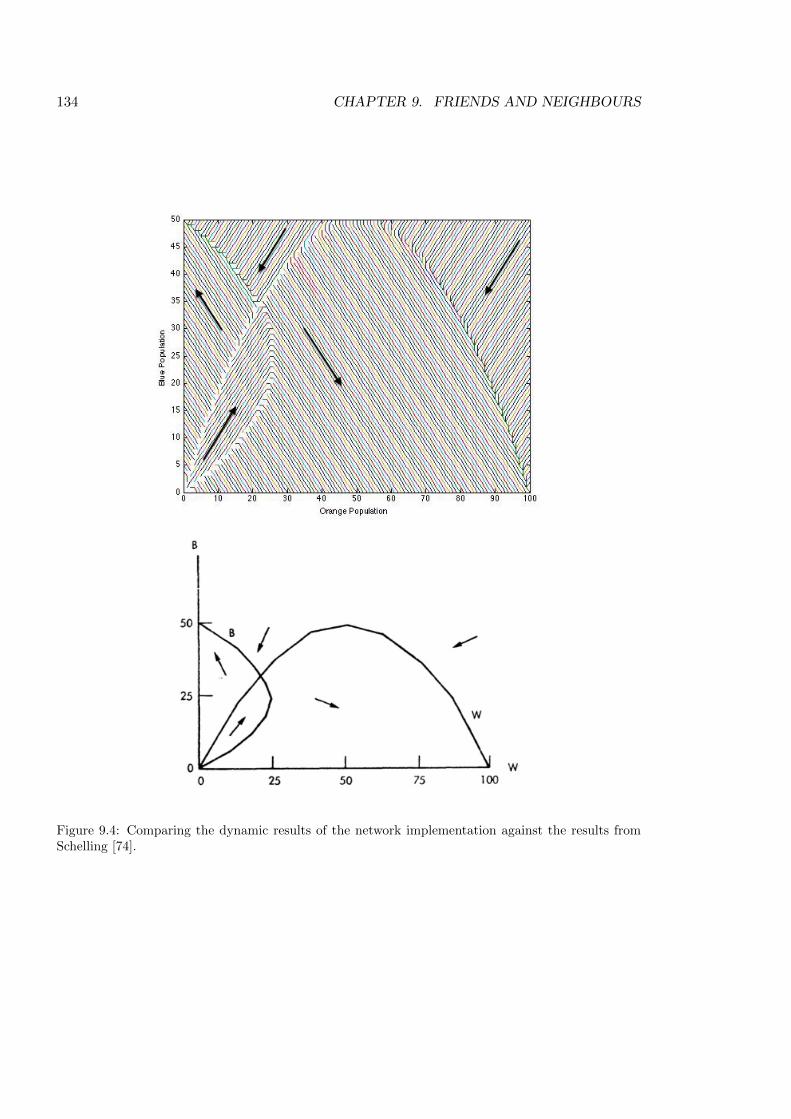
134 CHAPTER 9. FRIENDS AND NEIGHBOURS
Figure 9.4: Comparing the dynamic results of the network implementation against the results fromSchelling [74].
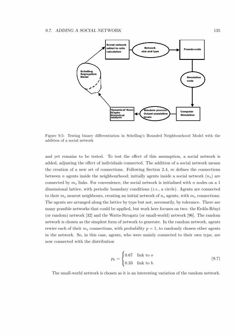
9.7. ADDING A SOCIAL NETWORK 135
Figure 9.5: Testing binary di↵erentiation in Schelling’s Bounded Neighbourhood Model with theaddition of a social network
and yet remains to be tested. To test the e↵ect of this assumption, a social network is
added, adjusting the e↵ect of individuals connected. The addition of a social network means
the creation of a new set of connections. Following Section 2.4, m defines the connections
between n agents inside the neighbourhood; initially agents inside a social network (ns) are
connected by ms links. For convenience, the social network is initialised with n nodes on a 1
dimensional lattice, with periodic boundary conditions (i.e., a circle). Agents are connected
to their ms nearest neighbours, creating an initial network of ns agents, with ms connections.
The agents are arranged along the lattice by type but not, necessarily, by tolerance. There are
many possible networks that could be applied, but work here focuses on two: the Erdos-Renyi
(or random) network [32] and the Watts-Strogatz (or small-world) network [96]. The random
network is chosen as the simplest form of network to generate. In the random network, agents
rewire each of their ms connections, with probability p = 1, to randomly chosen other agents
in the network. So, in this case, agents, who were mainly connected to their own type, are
now connected with the distribution
pk =
8<
:0.67 link to o
0.33 link to b.(9.7)
The small-world network is chosen as it is an interesting variation of the random network.
136 CHAPTER 9. FRIENDS AND NEIGHBOURS
For the small-world network, the initial connections are rewired according to a probability
p = 0.33. Thus the initial bias in the social networks is maintained, but one third of the
agents’ connections will be randomly distributed as described previously. Simple examples
of the initialisation and implementation of the two types of networks and their resulting ms
are shown in Figure 9.6. The small world network retains more of the order, with agents
more likely to be connected to their own type. The random network connections follow the
random distribution, with agents more likely to be connected to an agent of type O.
9.8 Hypothesis
The hypotheses tests the e↵ects of adding a social network to the model. We o↵er the
hypothesis that changing the movement will have an e↵ect on the outcome of the simulation.
This is tested by attempting to refute the null hypothesis (H0), that the change has no e↵ect,
using two measures, static and dynamic (discussed in Section 4.4).
9.8.1 Static measure
The static measure of the final population inside the neighbourhood, shows whether the
alteration to the model produces stable mixed populations. Following equation (4.1), M
is used to measure the final population configurations. The hypothesis, that changing the
movement rule will produce mixed populations, is tested by comparing M to Schelling’s
findings of M = 0. A result of M > 0 suggests mixed populations have arisen, counter to
Schelling’s model.
9.8.2 Dynamic measure
The analysis of the population flows focuses on I, which is the number of iterations taken to
reach a steady state. The system has reached a steady state when no more agents wish to
move. The results are analysed using the Mann-Whitney-Wilcoxon U test and the Vargha-
Delaney A-statistic, described in Section 4.4.
9.9 Domain model: adding a social network
The addition of a social network necessitates a change in the calculation of R. Agents of
the same type inside a social network are counted double, if and only if they are connected
to the neighbourhood component. Agents of the other type, inside a social network and
connected to the neighbourhood component are negated. As with Schelling’s model, agents
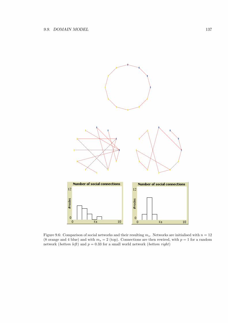
9.9. DOMAIN MODEL 137
Figure 9.6: Comparison of social networks and their resulting ms. Networks are initialised with n = 12(8 orange and 4 blue) and with ms = 2 (top). Connections are then rewired, with p = 1 for a randomnetwork (bottom left) and p = 0.33 for a small world network (bottom right)
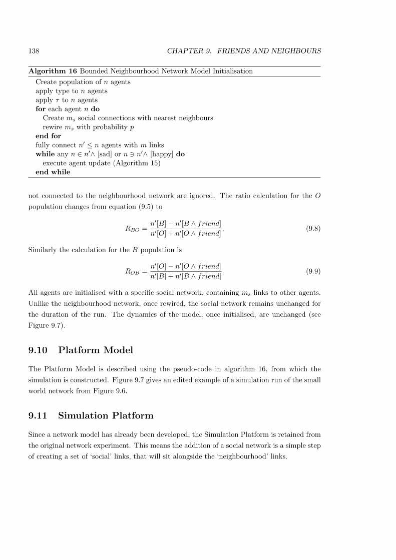
138 CHAPTER 9. FRIENDS AND NEIGHBOURS
Algorithm 16 Bounded Neighbourhood Network Model Initialisation
Create population of n agentsapply type to n agentsapply ⌧ to n agentsfor each agent n doCreate ms social connections with nearest neighboursrewire ms with probability p
end forfully connect n0
n agents with m linkswhile any n 2 n0
^ [sad] or n 3 n0^ [happy] do
execute agent update (Algorithm 15)end while
not connected to the neighbourhood network are ignored. The ratio calculation for the O
population changes from equation (9.5) to
RBO =n0[B]� n0[B ^ friend]
n0[O] + n0[O ^ friend]. (9.8)
Similarly the calculation for the B population is
ROB =n0[O]� n0[O ^ friend]
n0[B] + n0[B ^ friend]. (9.9)
All agents are initialised with a specific social network, containing ms links to other agents.
Unlike the neighbourhood network, once rewired, the social network remains unchanged for
the duration of the run. The dynamics of the model, once initialised, are unchanged (see
Figure 9.7).
9.10 Platform Model
The Platform Model is described using the pseudo-code in algorithm 16, from which the
simulation is constructed. Figure 9.7 gives an edited example of a simulation run of the small
world network from Figure 9.6.
9.11 Simulation Platform
Since a network model has already been developed, the Simulation Platform is retained from
the original network experiment. This means the addition of a social network is a simple step
of creating a set of ‘social’ links, that will sit alongside the ‘neighbourhood’ links.
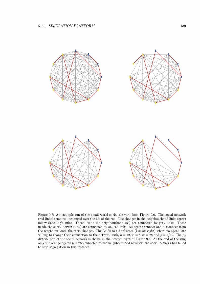
9.11. SIMULATION PLATFORM 139
Figure 9.7: An example run of the small world social network from Figure 9.6. The social network(red links) remains unchanged over the life of the run. The changes in the neighbourhood links (grey)follow Schelling’s rules. Those inside the neighbourhood (n0) are connected by grey links. Thoseinside the social network (ns) are connected by ms red links. As agents connect and disconnect fromthe neighbourhood, the ratio changes. This leads to a final state (bottom right) where no agents arewilling to change their connection to the network with, n = 12, n0 = 8,m = 28 and ⇢ = 7/12. The pkdistribution of the social network is shown in the bottom right of Figure 9.6. At the end of the run,only the orange agents remain connected to the neighbourhood network; the social network has failedto stop segregation in this instance.
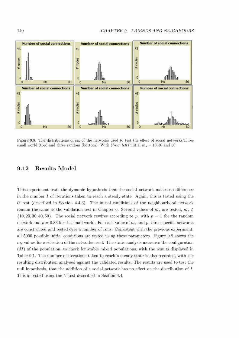
140 CHAPTER 9. FRIENDS AND NEIGHBOURS
Figure 9.8: The distributions of six of the networks used to test the e↵ect of social networks.Threesmall world (top) and three random (bottom). With (from left) initial ms = 10, 30 and 50.
9.12 Results Model
This experiment tests the dynamic hypothesis that the social network makes no di↵erence
in the number I of iterations taken to reach a steady state. Again, this is tested using the
U test (described in Section 4.4.3). The initial conditions of the neighbourhood network
remain the same as the validation test in Chapter 6. Several values of ms are tested, ms 2
{10, 20, 30, 40, 50}. The social network rewires according to p, with p = 1 for the random
network and p = 0.33 for the small world. For each value of ms and p, three specific networks
are constructed and tested over a number of runs. Consistent with the previous experiment,
all 5000 possible initial conditions are tested using these parameters. Figure 9.8 shows the
ms values for a selection of the networks used. The static analysis measures the configuration
(M) of the population, to check for stable mixed populations, with the results displayed in
Table 9.1. The number of iterations taken to reach a steady state is also recorded, with the
resulting distribution analysed against the validated results. The results are used to test the
null hypothesis, that the addition of a social network has no e↵ect on the distribution of I.
This is tested using the U test described in Section 4.4.
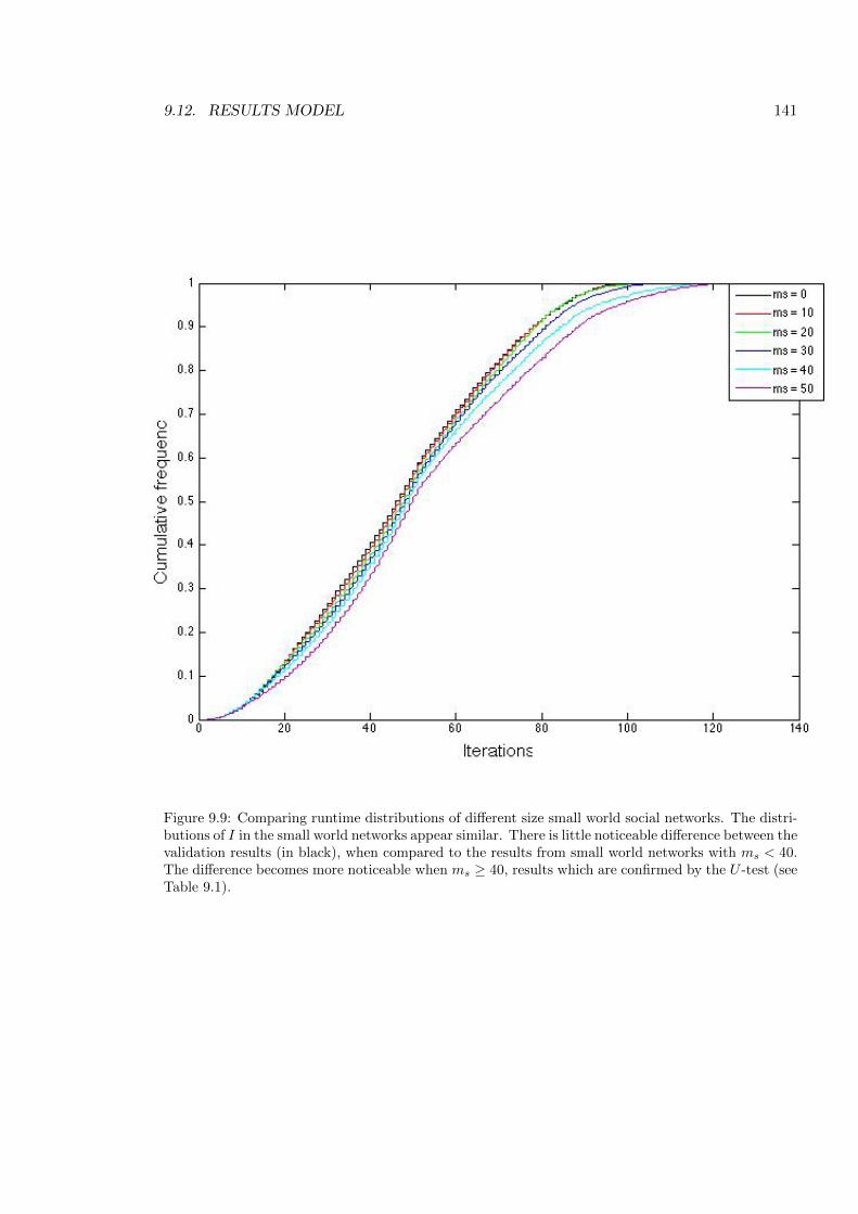
9.12. RESULTS MODEL 141
Figure 9.9: Comparing runtime distributions of di↵erent size small world social networks. The distri-butions of I in the small world networks appear similar. There is little noticeable di↵erence between thevalidation results (in black), when compared to the results from small world networks with ms < 40.The di↵erence becomes more noticeable when ms � 40, results which are confirmed by the U -test (seeTable 9.1).
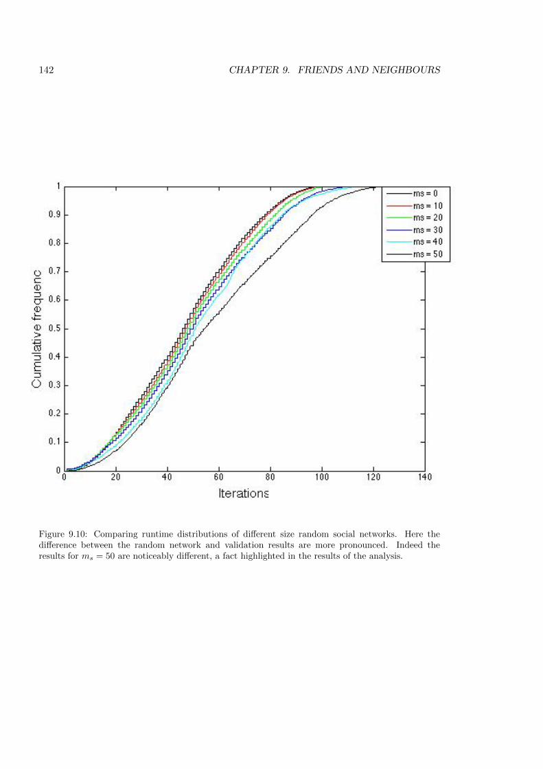
142 CHAPTER 9. FRIENDS AND NEIGHBOURS
Figure 9.10: Comparing runtime distributions of di↵erent size random social networks. Here thedi↵erence between the random network and validation results are more pronounced. Indeed theresults for ms = 50 are noticeably di↵erent, a fact highlighted in the results of the analysis.
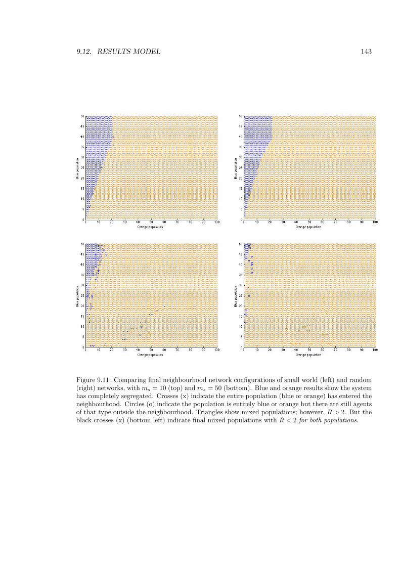
9.12. RESULTS MODEL 143
Figure 9.11: Comparing final neighbourhood network configurations of small world (left) and random(right) networks, with ms = 10 (top) and ms = 50 (bottom). Blue and orange results show the systemhas completely segregated. Crosses (x) indicate the entire population (blue or orange) has entered theneighbourhood. Circles (o) indicate the population is entirely blue or orange but there are still agentsof that type outside the neighbourhood. Triangles show mixed populations; however, R > 2. But theblack crosses (x) (bottom left) indicate final mixed populations with R < 2 for both populations.
144 CHAPTER 9. FRIENDS AND NEIGHBOURS
9.12.1 Appearance of mixed populations
Following work by Freeman [38], we define m⇤n as neighbourhood links connecting agents of
di↵erent type (i.e., blue with orange and vice-versa). The measure M of the segregation of
the population is now given as
M =m⇤
n
mn, (9.10)
thusM = 1 implies an equal mix andM = 0 complete segregation. Summing all theM values
and dividing by the number of samples in each run returns the mean M value. The results are
displayed in Table 9.1. Positive values of M imply that mixed populations exist; using their
initial conditions these points are mapped onto Figure 9.11. Since previous results of M > 0
were simply artefacts of the system reaching the maximum allowed number of iterations, it
is important to show that these populations are not in the process of segregating. This is
refuted by showing all the populations reaching a steady state (whereby no agents wishes to
move), before the number of iterations reaches the maximum. As Figures 9.9 and 9.10 show,
none of the runtimes come close to the maximum value of I. The population flows show
mixed population that have arisen not as an artefact of, either, an initial condition, or the
maximum I (as with Chapter 8).
The analysis of the runtime distributions highlights a di↵erence for both network sizes and
types (figures 9.9, 9.10). Statistical analysis suggests that, whilst the null hypothesis can be
rejected for social networks initialised with ms � 10; there is no e↵ect size until ms � 20 on
the random network, and none for the small world. While this suggests that the significant
results for ms < 20 are caused by the sample size, we have to reject the null hypothesis.
However the A statistic shows no e↵ect size for the small world networks and only appears
when ms � 20. A representative sample of results are displayed in table 9.1. Results with an
e↵ect size are displayed in bold.
Although the social networks have to reach a relatively large size before having a no-
ticeable e↵ect on the simulation runtime, both types of social networks are able to maintain
stable mixed populations (M > 0) for smaller values of ms. This is the first time the Bounded
Neighbourhood Model has produced stable mixed populations using Schelling’s original pa-
rameters. These results are shown in red in Figure 9.11.
In addition, the density ⇢ of the mixed neighbourhood networks gives an indication of the
stability of the network. A network with a higher density is less likely to be a↵ected by the
changes caused by a single agent moving. Plotting M against ⇢ gives a clearer picture of the
neighbourhood network. As can be seen in Figure 9.12, the highest value of ⇢ corresponds to
the lowest value of M . When M = 0, ⇢ = 0.66 or 0.33, corresponding to the neighbourhood
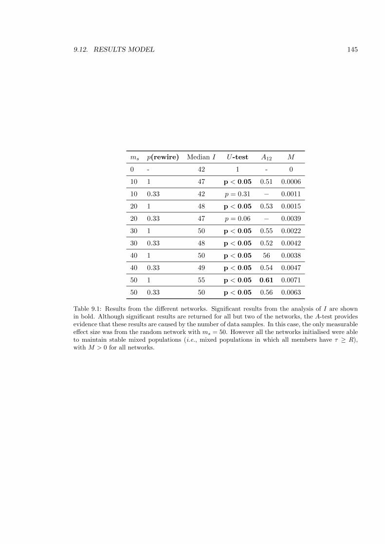
9.12. RESULTS MODEL 145
ms p(rewire) Median I U-test A12 M
0 - 42 1 - 0
10 1 47 p < 0.05 0.51 0.0006
10 0.33 42 p = 0.31 � 0.0011
20 1 48 p < 0.05 0.53 0.0015
20 0.33 47 p = 0.06 � 0.0039
30 1 50 p < 0.05 0.55 0.0022
30 0.33 48 p < 0.05 0.52 0.0042
40 1 50 p < 0.05 56 0.0038
40 0.33 49 p < 0.05 0.54 0.0047
50 1 55 p < 0.05 0.61 0.0071
50 0.33 50 p < 0.05 0.56 0.0063
Table 9.1: Results from the di↵erent networks. Significant results from the analysis of I are shownin bold. Although significant results are returned for all but two of the networks, the A-test providesevidence that these results are caused by the number of data samples. In this case, the only measurablee↵ect size was from the random network with ms = 50. However all the networks initialised were ableto maintain stable mixed populations (i.e., mixed populations in which all members have ⌧ � R),with M > 0 for all networks.
146 CHAPTER 9. FRIENDS AND NEIGHBOURS
network either being all orange or all blue respectively. It is interesting to note that ⇢ increases
as the size of the social network increases, however M gets smaller. This suggests that larger
networks are able to sustain populations with higher levels of segregation.
9.13 Conclusions
By translating the Bounded Neighbourhood Model as a network, we have been able to add
a social network, allowing investigation into the e↵ect of binary di↵erentiation. The results
show that integrated populations are possible within the Bounded Neighbourhood Model. In
addition, according to the Vargha-Delaneytest results the random social network significantly
changes the time taken for the simulation to reach a steady state (although the e↵ect size
is small). As ms increases, fewer runs terminate with the minority population inside the
neighbourhood. In fact when ms = 50 and p = 1, the minority population are unable to
maintain a segregated population, even when the initialisation is heavily their favour (lower
right diagram in Figure 9.11). The majority population manages to maintain itself. This is
because, when the social network is the size of the minority population (i.e., 50), the majority
population will be able to ignore them completely (50 � 50 = 0). In contrast, the minority
population can, at best, ignore only half of the majority population (100� 50 = 50).
9.13.1 Appearance of integrated populations
A number of mixed populations remained unchanged over the runtime. Although these fixed
points existed, no other populations flowed into them. This suggests they are fixed points
that are di�cult to reach from other initial conditions. The fact that the small world network
was unable to match the e↵ect of the random network, suggests the bias of type in the social
network has an e↵ect and is certainly an area for further exploration. The creation of mixed
steady states (M > 0) is a novel result from the Schelling model. This provides evidence
that the model can support mixed populations without explicitly altering the tolerance or
population parameters. It is interesting to note that, although the small world network does
not cause a significant di↵erence in the runtime, it results in more integrated populations
than the random network (Ssw > Sr). The density of the final networks has a maximum
of ⇢ = 0.66, which corresponds to a network with 100 out of 150 agents connected. Thus,
although the social network is able to produce mixed populations, it is unable to create
mixed neighbourhood networks with a density higher than 0.6. However, the fact that the
simulation produces mixed populations at all is an important result, since this is the first
time Schelling’s Bounded Neighbourhood Model has produced stable integrated populations.
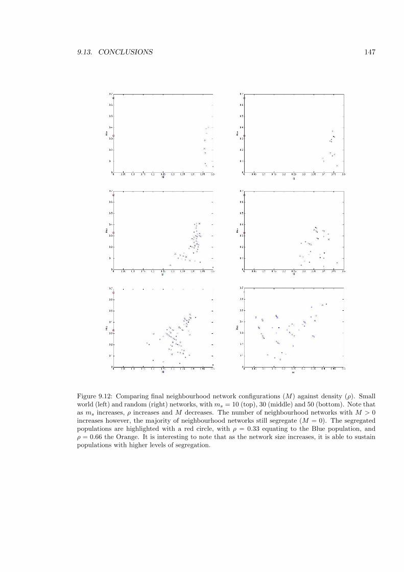
9.13. CONCLUSIONS 147
Figure 9.12: Comparing final neighbourhood network configurations (M) against density (⇢). Smallworld (left) and random (right) networks, withms = 10 (top), 30 (middle) and 50 (bottom). Note thatas ms increases, ⇢ increases and M decreases. The number of neighbourhood networks with M > 0increases however, the majority of neighbourhood networks still segregate (M = 0). The segregatedpopulations are highlighted with a red circle, with ⇢ = 0.33 equating to the Blue population, and⇢ = 0.66 the Orange. It is interesting to note that as the network size increases, it is able to sustainpopulations with higher levels of segregation.

148 CHAPTER 9. FRIENDS AND NEIGHBOURS
Chapter 10
Conclusions and Further work
Schelling’s seminal segregation models helped to found the field of Computational Social
Science. With well over 2000 citations, the influence of the models is matched only by Sug-
arscape [4]. However, the majority of work on his models has focused on the Spatial Proximity
Model, where the environment is represented as a grid of cells (discussed in Chapter 3.1).
This thesis has explored the less well known, but no less interesting, Bounded Neighbour-
hood Model. Schelling himself asked why there has been so little research into the Bounded
Neighbourhood Model [76]. Claims by Hatna et al. that the Bounded Neighbourhood Model
has been “analytically investigated” [46, p6], by Schelling [75] and Clark [23], [24] may be
the explanation. However the investigation by Clark was limited to discussing the Bounded
Neighbourhood Model as a variant of the Spatial Proximity Model. Indeed in [24], the model
developed is an exploration of the “Schelling segregation model”, with no consideration of
the Bounded Neighbourhood Model. His argument, that the model has been mathematically
solved, is based on Zhang’s game theoretical description of the Spatial Proximity Model, in
which the tolerance is the same for all individuals in a particular population, and so does
not apply to the Bounded Neighbourhood Model. It is also possible that there is confusion
over the models that has arisen from the terms ‘Schelling segregation’ and Spatial Proximity
Model being used interchangeably. Fossett [37] claims his simulation “SimSeg” is a simula-
tion of a combined Spatial Proximity Model and Bounded Neighbourhood Model. Although
adjusting the spatial parameters can result in a bounded neighbourhood on the system, the
agents’ tolerance remains identical, as required by the Spatial Proximity Model. Although
Fossett’s model can vary the tolerance between groups (i.e., blacks are more tolerant than
whites), there is no variation within the groups (i.e., all blacks have the same tolerance).
However one of the defining characteristics of the Bounded Neighbourhood Model is individ-
ually variable tolerance, in which each agent within a group has a unique level of tolerance
149
150 CHAPTER 10. CONCLUSIONS AND FURTHER WORK
(see Section 3.2).
The analyses presented here have shown that the behaviour of the Bounded Neighbour-
hood Model exhibits a remarkable resistance to changes in the parameters. For many (e.g.,
[15], [37], [23]) this is a vindication of the strength of the model. However, applying the model
to real world segregation requires a much greater understanding of the model (not to mention
reality). Nevertheless, taken as a tool to explore ideas of segregation, Schelling’s model has
been widely used as an example of how even relatively low levels of intolerance, in a simple
population, can create highly segregated populations. Attempts to apply Schelling’s model
to real world areas has, rightly, created much debate. Benenson and Hatna [15] and [46]
use Schelling’s model to explain segregation in certain Israeli cities. However, as with many
segregation models that use Schelling’s model, some of Schelling’s assumptions are ignored.
Indeed more assumptions are added in [15] (see Section 2.6). In addition there is rarely any
consideration of individual adaption in the models. Thus, even though the system changes
over time, the agents can only change their location. An obvious comparison is Sugarscape
where, a simple inheritance rule allows adaption, such as the aggregation of wealth. However,
Schelling’s segregation models involve no adaption of the agents’ behaviour at all.
10.1 Summary of Results
The work in this thesis has examined Schelling’s Bounded Neighbourhood Model. No at-
tempt has been made to relate it to any ‘real-world’ social system. Instead, following the
CoSMoS process, experiments have been performed to first understand, and then probe cer-
tain key aspects of the model. This process eventually led to the development of the network
model (chapter 9) which exhibited the emergence of stable mixed populations. The develop-
ment of the formalisation brings out some hitherto unexplored assumptions in the Bounded
Neighbourhood Model (Chapter 5) and the results from the simulation were used to validate
further variations of the model. Schelling’s four basic assumptions, namely movement order
(Chapter 6), perfect knowledge (Chapter 7), perfect response (Chapter 8) and homogeneous
populations (Chapter 9) are set out and their analysis briefly reviewed below.
For each experiment, two measures were used to test the model. One static, analysing
final population mixtures, and one dynamic, analysing population movement over time. The
static measure calculated the final population configurations of Schelling’s model, using a
parameter M that defines the mix of the population (where M = 1 indicates a 50/50 mix).
This type of final state measure is often used when analysing Schelling segregation models
(for example [15],[17] and [53]). However, in reality, systems are in constant flux, making an
analysis of the dynamics of the system desirable. By measuring the number of iterations the
10.1. SUMMARY OF RESULTS 151
system took to reach equilibrium, the dynamics of the model can be analysed (see Section
4.4). In addition, taking two perspectives in the analysis gives a better understanding of the
model.
10.1.1 Changing the movement order: Whose move is it anyway?
In Chapter 6, Schelling’s assumption that agents moved in order of their tolerance was exam-
ined. Using the formalisation and simulation developed in Chapter 5, a validated change to
the movement rule was implemented. By choosing the agents in order of tolerance, the sim-
ulation replicated Schelling’s flows; while choosing at random produced more chaotic flows
(Figure 6.3). The e↵ects of the change were measured and analysed using a U test (see
Section 4.4) on the hypotheses:
Static measure M
The static measure analysed the robustness of segregation in the model, in response to changes
in the movement order. In this experiment, changing the order of the movement had no
discernible e↵ect on the final population mix, all populations ended with complete segregation
(M = 0).
Dynamic measure I
The dynamic hypothesis tested the number I of iterations taken for the simulation to reach a
‘steady state’ (as defined in Section 4.4). When agents were chosen to move at random, the
number of iterations increased. The U test returned a significant result with the follow up A
statistic returning a large e↵ect size. This confirms the expectation that the time taken to
reach a steady state can be increased by randomising the movement of the agents.
Results of the simulation: M = 0, but increased I.
Although the median value of I for the random movement was larger than the deterministic
model, for both cases, every steady state was completely segregated with M = 0. The
results from the experiment (summarised in table 10.1) show that the final populations always
segregate regardless of the order of movement, although the number of iterations to reach
segregation is increased.
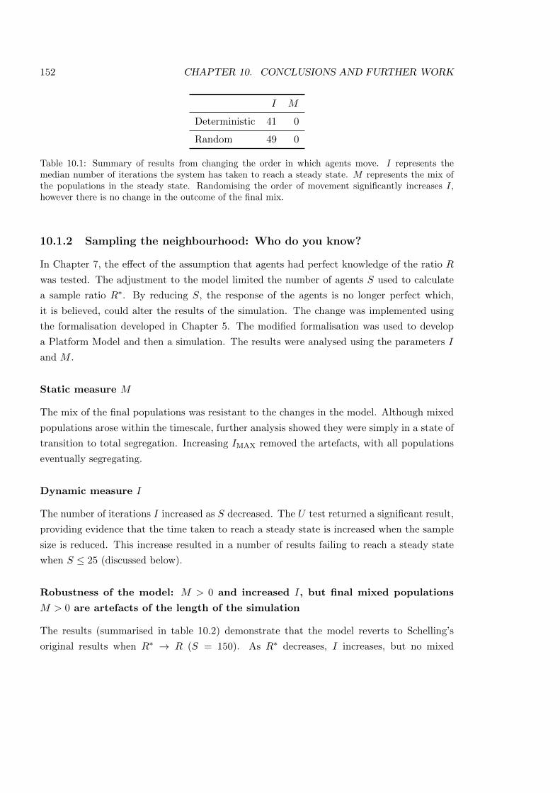
152 CHAPTER 10. CONCLUSIONS AND FURTHER WORK
I M
Deterministic 41 0
Random 49 0
Table 10.1: Summary of results from changing the order in which agents move. I represents themedian number of iterations the system has taken to reach a steady state. M represents the mix ofthe populations in the steady state. Randomising the order of movement significantly increases I,however there is no change in the outcome of the final mix.
10.1.2 Sampling the neighbourhood: Who do you know?
In Chapter 7, the e↵ect of the assumption that agents had perfect knowledge of the ratio R
was tested. The adjustment to the model limited the number of agents S used to calculate
a sample ratio R⇤. By reducing S, the response of the agents is no longer perfect which,
it is believed, could alter the results of the simulation. The change was implemented using
the formalisation developed in Chapter 5. The modified formalisation was used to develop
a Platform Model and then a simulation. The results were analysed using the parameters I
and M .
Static measure M
The mix of the final populations was resistant to the changes in the model. Although mixed
populations arose within the timescale, further analysis showed they were simply in a state of
transition to total segregation. Increasing IMAX removed the artefacts, with all populations
eventually segregating.
Dynamic measure I
The number of iterations I increased as S decreased. The U test returned a significant result,
providing evidence that the time taken to reach a steady state is increased when the sample
size is reduced. This increase resulted in a number of results failing to reach a steady state
when S 25 (discussed below).
Robustness of the model: M > 0 and increased I, but final mixed populations
M > 0 are artefacts of the length of the simulation
The results (summarised in table 10.2) demonstrate that the model reverts to Schelling’s
original results when R⇤! R (S = 150). As R⇤ decreases, I increases, but no mixed
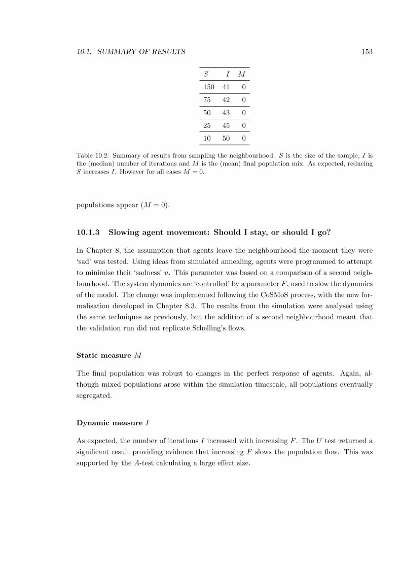
10.1. SUMMARY OF RESULTS 153
S I M
150 41 0
75 42 0
50 43 0
25 45 0
10 50 0
Table 10.2: Summary of results from sampling the neighbourhood. S is the size of the sample, I isthe (median) number of iterations and M is the (mean) final population mix. As expected, reducingS increases I. However for all cases M = 0.
populations appear (M = 0).
10.1.3 Slowing agent movement: Should I stay, or should I go?
In Chapter 8, the assumption that agents leave the neighbourhood the moment they were
‘sad’ was tested. Using ideas from simulated annealing, agents were programmed to attempt
to minimise their ‘sadness’ u. This parameter was based on a comparison of a second neigh-
bourhood. The system dynamics are ‘controlled’ by a parameter F , used to slow the dynamics
of the model. The change was implemented following the CoSMoS process, with the new for-
malisation developed in Chapter 8.3. The results from the simulation were analysed using
the same techniques as previously, but the addition of a second neighbourhood meant that
the validation run did not replicate Schelling’s flows.
Static measure M
The final population was robust to changes in the perfect response of agents. Again, al-
though mixed populations arose within the simulation timescale, all populations eventually
segregated.
Dynamic measure I
As expected, the number of iterations I increased with increasing F . The U test returned a
significant result providing evidence that increasing F slows the population flow. This was
supported by the A-test calculating a large e↵ect size.
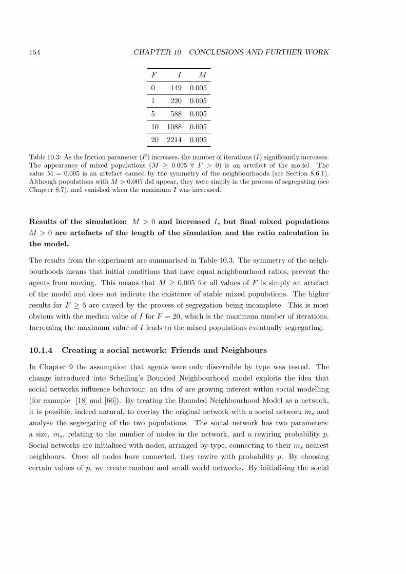
154 CHAPTER 10. CONCLUSIONS AND FURTHER WORK
F I M
0 149 0.005
1 220 0.005
5 588 0.005
10 1088 0.005
20 2214 0.005
Table 10.3: As the friction parameter (F ) increases, the number of iterations (I) significantly increases.The appearance of mixed populations (M � 0.005 8 F > 0) is an artefact of the model. Thevalue M = 0.005 is an artefact caused by the symmetry of the neighbourhoods (see Section 8.6.1).Although populations with M > 0.005 did appear, they were simply in the process of segregating (seeChapter 8.7), and vanished when the maximum I was increased.
Results of the simulation: M > 0 and increased I, but final mixed populations
M > 0 are artefacts of the length of the simulation and the ratio calculation in
the model.
The results from the experiment are summarised in Table 10.3. The symmetry of the neigh-
bourhoods means that initial conditions that have equal neighbourhood ratios, prevent the
agents from moving. This means that M � 0.005 for all values of F is simply an artefact
of the model and does not indicate the existence of stable mixed populations. The higher
results for F � 5 are caused by the process of segregation being incomplete. This is most
obvious with the median value of I for F = 20, which is the maximum number of iterations.
Increasing the maximum value of I leads to the mixed populations eventually segregating.
10.1.4 Creating a social network: Friends and Neighbours
In Chapter 9 the assumption that agents were only discernible by type was tested. The
change introduced into Schelling’s Bounded Neighbourhood model exploits the idea that
social networks influence behaviour, an idea of are growing interest within social modelling
(for example [18] and [66]). By treating the Bounded Neighbourhood Model as a network,
it is possible, indeed natural, to overlay the original network with a social network ms and
analyse the segregating of the two populations. The social network has two parameters:
a size, ms, relating to the number of nodes in the network, and a rewiring probability p.
Social networks are initialised with nodes, arranged by type, connecting to their ms nearest
neighbours. Once all nodes have connected, they rewire with probability p. By choosing
certain values of p, we create random and small world networks. By initialising the social
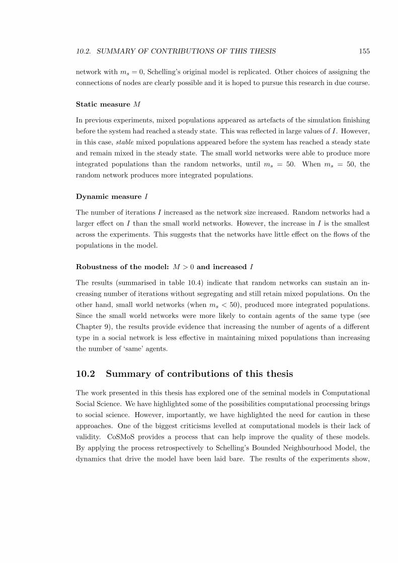
10.2. SUMMARY OF CONTRIBUTIONS OF THIS THESIS 155
network with ms = 0, Schelling’s original model is replicated. Other choices of assigning the
connections of nodes are clearly possible and it is hoped to pursue this research in due course.
Static measure M
In previous experiments, mixed populations appeared as artefacts of the simulation finishing
before the system had reached a steady state. This was reflected in large values of I. However,
in this case, stable mixed populations appeared before the system has reached a steady state
and remain mixed in the steady state. The small world networks were able to produce more
integrated populations than the random networks, until ms = 50. When ms = 50, the
random network produces more integrated populations.
Dynamic measure I
The number of iterations I increased as the network size increased. Random networks had a
larger e↵ect on I than the small world networks. However, the increase in I is the smallest
across the experiments. This suggests that the networks have little e↵ect on the flows of the
populations in the model.
Robustness of the model: M > 0 and increased I
The results (summarised in table 10.4) indicate that random networks can sustain an in-
creasing number of iterations without segregating and still retain mixed populations. On the
other hand, small world networks (when ms < 50), produced more integrated populations.
Since the small world networks were more likely to contain agents of the same type (see
Chapter 9), the results provide evidence that increasing the number of agents of a di↵erent
type in a social network is less e↵ective in maintaining mixed populations than increasing
the number of ‘same’ agents.
10.2 Summary of contributions of this thesis
The work presented in this thesis has explored one of the seminal models in Computational
Social Science. We have highlighted some of the possibilities computational processing brings
to social science. However, importantly, we have highlighted the need for caution in these
approaches. One of the biggest criticisms levelled at computational models is their lack of
validity. CoSMoS provides a process that can help improve the quality of these models.
By applying the process retrospectively to Schelling’s Bounded Neighbourhood Model, the
dynamics that drive the model have been laid bare. The results of the experiments show,
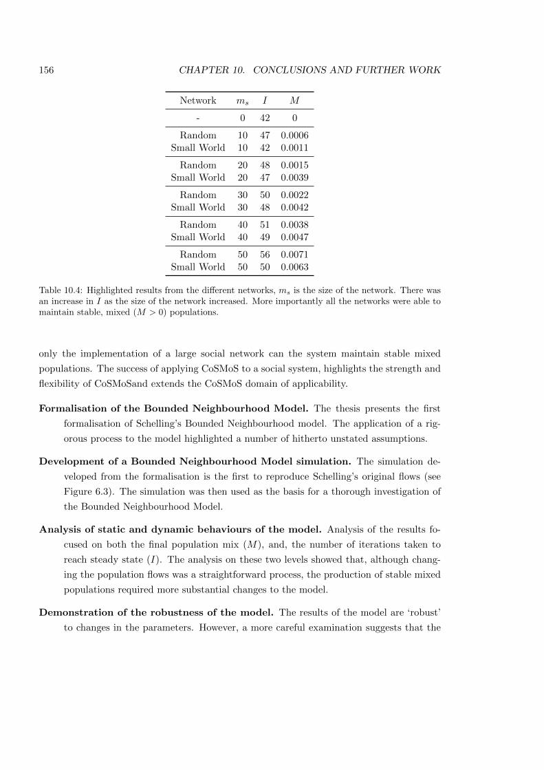
156 CHAPTER 10. CONCLUSIONS AND FURTHER WORK
Network ms I M
- 0 42 0
Random 10 47 0.0006Small World 10 42 0.0011
Random 20 48 0.0015Small World 20 47 0.0039
Random 30 50 0.0022Small World 30 48 0.0042
Random 40 51 0.0038Small World 40 49 0.0047
Random 50 56 0.0071Small World 50 50 0.0063
Table 10.4: Highlighted results from the di↵erent networks, ms is the size of the network. There wasan increase in I as the size of the network increased. More importantly all the networks were able tomaintain stable, mixed (M > 0) populations.
only the implementation of a large social network can the system maintain stable mixed
populations. The success of applying CoSMoS to a social system, highlights the strength and
flexibility of CoSMoSand extends the CoSMoS domain of applicability.
Formalisation of the Bounded Neighbourhood Model. The thesis presents the first
formalisation of Schelling’s Bounded Neighbourhood model. The application of a rig-
orous process to the model highlighted a number of hitherto unstated assumptions.
Development of a Bounded Neighbourhood Model simulation. The simulation de-
veloped from the formalisation is the first to reproduce Schelling’s original flows (see
Figure 6.3). The simulation was then used as the basis for a thorough investigation of
the Bounded Neighbourhood Model.
Analysis of static and dynamic behaviours of the model. Analysis of the results fo-
cused on both the final population mix (M), and, the number of iterations taken to
reach steady state (I). The analysis on these two levels showed that, although chang-
ing the population flows was a straightforward process, the production of stable mixed
populations required more substantial changes to the model.
Demonstration of the robustness of the model. The results of the model are ‘robust’
to changes in the parameters. However, a more careful examination suggests that the
10.3. FURTHER WORK 157
results are by construction, rather than by emergence. The parameters drive the model
to segregation rather than allowing segregation to emerge. This hardwiring of the model
is not immediately obvious and it has taken a thorough investigation to highlight the
issue. This result has important implications for the use of the Bounded Neighbourhood
Model in discussions of the determinants of segregation in social studies.
Demonstration of e↵ect of social networks on segregation in the model. The demon-
stration that the addition of a social network produces stable, integrated, populations is
more evidence of why not to apply the model blindly to real world situations. However
Schelling’s Bounded Neighbourhood Model still has utility and is an excellent segrega-
tion model.
10.3 Further work
Clearly Schelling’s models have a plethora of possible future research ideas, some of which
were examined in Chapter 3.6. The work presented in this thesis is a first step in a systematic
exploration of Schelling’s Bounded Neighbourhood model and related models. Further work
could develop some of the questions raised in this study. For example:
Heterogeneous populations. Further work could use the model developed in Chapter 9
and explore the e↵ects of di↵erent types within populations.
Space. The network model is a first step in the introduction of space into the Bounded
Neighbourhood Model. The treatment of space is an important aspect of social science
(especially urban studies). However, Schelling’s models have a complete disregard for
anything other than uniform space. It would be interesting to examine if changing the
perceptions of space in the model would e↵ect the outcomes.
Timescales. Further exploration of the movement rule could explore the e↵ect of agents
moving at di↵erent timescales, either individually or by type.
Time decay for social bonds. Linked to timescales, would a social bond that decayed
over time e↵ect the results of the network model?
Ratio calculations Although Chapter 7 explored ideas of agents calculating di↵erent ratios
from the same population, further work could explore ideas of agents retaining their
calculated ratio for a period of time, rather than recalculating at each iteration?
Population adaption. The character of the members in the populations undergoes no
change in Schelling’s models and the Bounded Neighbourhood Model in particular.

158 CHAPTER 10. CONCLUSIONS AND FURTHER WORK
This is a serious limitation and leads one to ask what e↵ects an evolutionary model
could have on a Schelling segregation model?
These are just a few of the many questions the formalisation and testing of Schelling’s
Bounded Neighbourhood Model has promted. The thorough examination presented here
has given an insight into the key drivers of the model. The further work described is merely
the beginning of what is sure to be a rich field of research.
Bibliography
[1] Colorbrewer, http://colorbrewer2.org, December 2013.
[2] The Journal of Artificial Societies and Social Simulation,
http://jasss.soc.surrey.ac.uk/jasss.html, March 2014.
[3] Netlogo, http://ccl.northwestern.edu/netlogo, January 2014.
[4] Sugarscape, http://sugarscape.sourceforge.net, October 2012.
[5] A. J. Lotka, http://www.eoearth.org/view/article/51cbee5a7896bb431f6973ee/,
November 2010.
[6] K. Alden, J. Timmis, P. S. Andrews, H. Veiga-Fernandes, and M. C. Coles. Pairing
experimentation and computational modeling to understand the role of tissue inducer
cells in the development of lymphoid organs. Frontiers in immunology, 3(172), 2012.
[7] P. S. Andrews, F. A. C. Polack, A. T. Sampson, S. Stepney, and J. Timmis. The
CoSMoS Process, Version 0.1: A Process for the Modelling and Simulation of Complex
Systems. Technical Report YCS-2010-453, University of York, 2010.
[8] A. Arcuri and L. Briand. A Hitchhiker’s Guide to Statistical Tests for Assessing Ran-
domized Algorithms in Software Engineering. Technical Report 2011-13, Simula Re-
search Laboratory, P.O. Box 134, Lysaker, Norway, 2011.
[9] Aristotle. Aristotle’s Metaphysics, volume translation by W Ross. Oxford University
Press, 1924.
[10] R. Axelrod. Advancing the art of simulation in the Social Sciences. Japanese Journal
for Management Information System, 12(3):1–19, December 2003.
[11] P. Bak, K. Chen, and M. Creutz. Self-organized criticality in the ‘Game of Life’. Nature,
342(6251):780–782, December 1989.
159
160 BIBLIOGRAPHY
[12] M. Batty. Agent-based pedestrian modelling. Advanced spatial analysis: the CASA
book of GIS, page 81, 2003.
[13] M. Bedau. Weak Emergence. Philosophical Perspectives 11: Mind, Causation and
World, 31(11):375–399, 1997.
[14] R. D. Beer. A dynamical systems perspective on agent-environment interaction. Arti-
ficial Intelligence, 72(1-2):173–215, 1995.
[15] I. Benenson and E. Hatna. The third state of the Schelling model of residential dynam-
ics. Arxiv preprint arXiv:0910.2414, 2009.
[16] I. Benenson, E. Hatna, and E. Or. From Schelling to spatially explicit modeling of
urban ethnic and economic residential dynamics. Sociological Methods & Research,
37(4):463–497, May 2009.
[17] J. M. Benito and P. Hernandez. Schelling’s dynamic models of segregation: a cellular
automata approach’. XXIX Simposio de Analisis Economico, Universidad de Navara,
2004.
[18] N. W. F. Bode, A. J. Wood, and D. W. Franks. The impact of social networks on
animal collective motion. Animal Behaviour, 82(1):29–38, 2011.
[19] J. Bown, P. S. Andrews, Y. Denni, A. Goltsov, M. Idowu, F. A. C. Polack, A. T.
Sampson, M. Shovman, and S. Stepney. Engineering Simulations for Cancer Systems
Biology. Current Drug Targets, 13(12):1560–1574, 2012.
[20] G. E. P. Box and N. R. Draper. Empirical Model-Building and Response Surfaces.
Wiley, 1987.
[21] D. Byrne. Complexity Theory and the Social Sciences: An Introduction. Routledge,
1998.
[22] J. L. Casti and A. Karlqvist, editors. Complexity, Language and Life: Mathematical
Approaches, volume 16. Springer-Verlag, 1980.
[23] W. A. V. Clark. Ethnic preferences and residential segregation: A commentary on
outcomes from agent-based modeling. The Journal of Mathematical Sociology, 30(3-
4):319–326, 2006.
BIBLIOGRAPHY 161
[24] W. A. V. Clark and M. Fossett. Understanding the social context of the Schelling
segregation model. Proceedings of the National Academy of Sciences, 105(11):4109,
2008.
[25] J. E. Cohen, T. Jonsson, and S. R. Carpenter. Ecological community description using
the food web, species abunance and body size. Proceedings of the National Academy of
Sciences, 100(4):1781–1786, Feb 2003.
[26] J. Corbett, G. Rambaldi, P. Kyem, D. Weiner, R. Olson, J. Muchemi, M. McCall,
and R. Chambers. Overview: Mapping for change - the emergence of a new practice.
Participatory Learning and Action, 54(1):13–19, 2006.
[27] A. Drogoul and J. Ferber. Multi-agent simulation as a tool for studying emergent
processes in society. Proceedings of Simulating Societies: The computer simulation of
social phenomena, LNCS, 830:2–23, 1994.
[28] W. Easterly. Empirics of strategic interdependence: the case of the racial tipping point.
The B.E. Journal of Macroeconomics, 9(1):1–33 (Article 25), 2009.
[29] J. M. Epstein. Generative Social Science - Studies in Agent-Based Modeling. Princton
University Press, 2006.
[30] J. M. Epstein. Why model? Journal of Artificial Societies and Social Simulation,
11(4):12, 2008.
[31] J. M. Epstein and R. Axtell. Growing Artificial Societies - Social science from the
bottom up. Brooking Institute Press, 1996.
[32] P. Erdos and Renyi A. On the evolution of random graphs. Publ. Mathematical Institute
of Hungarian Academic Sciences, 5:17–61, 1960.
[33] R. Eve, M. Lee, and S. Horsfall. Chaos, complexity, and sociology: myths, models, and
theories. SAGE Publications, 1997.
[34] R. Farley, E. Fielding, and M. Krysian. The residential preferences of blacks and whites:
A four-metropolis analysis. Housing Policy Debate, 8(4):763–800, 1997.
[35] R. Farley, H. Schuman, S. Bianchi, D. Colsanto, and S. Hatchett. Chocolate city, vanilla
suburbs: Will the trend toward racially seperate communities continue? Social Science
Research, 7:319–344, 1978.
162 BIBLIOGRAPHY
[36] A. Flache and R. Hegselmann. Do irregular grids make a di↵erence? Relaxing the
spatial regularity assumption in cellular models of social dynamics. Journal of Artificial
Societies and Social Simulation, 4(4), 2001.
[37] M. Fossett. Ethnic preferences, social distance dynamics and residential segregation.
Presented at the Annual Meetings of the American Sociological Association, March
1999.
[38] L. C. Freeman. Segregation in social networks. Sociological Methods and Research,
6:411–429, 1978.
[39] J M Galan, L R Izquierdo, S S Izquierdo, R del Olmo, A Lopez-Paredes, and B Ed-
monds. Errors and artefacts in agent-based modelling. Journal of Artificial Societies
and Social Simulation, 12(1):1, 2009.
[40] M. Gardner. Mathematical games: The fantastic combinations of John Conway’s new
solitaire game ‘Life’. Scientific American, 223(4):120–123, 1970.
[41] P. Garnett, S. Stepney, F. Day, and O. Leyser. Using the CoSMoS Process to enhance
an executable model of auxin transport canalisation. In CoSMoS 2010: Proceedings of
the 2010 Workshop on Complex Systems Modelling and Simulation, pages 9–32, 2010.
[42] N. Geard and S. Bullock. Competition and the dynamics of group a�liation. Advances
in Complex Systems, 13(4):501–507, 2010.
[43] N Gilbert and J Doran. Simulating societies: The computer simulation of social phe-
nomena. Routledge, 1994.
[44] A Gorban, I Karlin, and A Zinovyev. Invariant Grids: Method of Complexity Reduction
in Reaction Networks. Complexus, 2:110–127, Aug 2006.
[45] L. Hamill and N. Gilbert. Simulating large Social Networks in Agent-Based Models: A
Social Circle Model. Emergence: Complexity and Organization, 12(4):78–94, 2010.
[46] E. Hatna and I. Benenson. The Schelling model of ethnic residential dynamics: Beyond
the integrated - segregated dichotomy of patterns. Journal of Artificial Societies and
Social Simulation, 15(1):6, 2012.
[47] R E Hodel. An Introduction to Mathematical Logic. 1995.
[48] D Hosler, J A Sablo↵, and D Runge. Simulation model development: a case study of
the Classical Mayan collapse, pages 552–590. 1977.
BIBLIOGRAPHY 163
[49] T. Hoverd and S. Stepney. Environment orientation: an architecture for simulating
complex systems. CoSMoS 2009, pages 67–82, 2009.
[50] S. Kau↵man. At home in the universe. Viking, 1995.
[51] D. Kivotides and A. Leonard. Quantized turbulence physics. Phys. Rev. Lett,
90(23):234503, Jun 2003.
[52] C. Langton. Computation at the edge of chaos: Phase transitions and emergent com-
putation. Physica D: Nonlinear Phenomena, 42(1-3):12–37, 1990.
[53] A. J. Laurie and N. K. Jaggi. Role of ‘vision’ in neighbourhood racial segregation: A
variant of the Schelling segregation model. Urban Studies, 40(13):2687–2704, 2003.
[54] E R Leigh. Some Mathematical Problems in Biology. American Mathematical Society,
1968.
[55] S. Lloyd and H. Pagels. Complexity as thermodynamic depth. Annals of Physics,
188(1):186–213, Nov 1988.
[56] P. A. Longley, M. F. Goodchild, D. J. Maguire, and D. W. Rhind. Geographic Infor-
mation Systems and Science. Wiley, 2001.
[57] M. Macy and R. Willer. From factors to actors: Computational Sociology and Agent-
Based Modeling. Annual Review of Sociology, 28(143-166), Jan 2002.
[58] D. S. Massey and N. A. Denton. American apartheid: segregation and the making of
the underclass. Harvard University Press, 1993.
[59] Mathworld. Di↵erence equation, http://mathworld.wolfram.com/recurrenceequation.html,
Sep 2009.
[60] A. J. Mayer. Russel Woods : Change without conflict. Studies in housing and minority
groups, 1960.
[61] F. Mazzocchi. Complexity in Biology. EMBO Reports, 9(1):10–14, 2008.
[62] M. Newman, A-L Barabasi, and D. J. Watts. The Structure and Dynamics of Network-
setworks. Princeton Studies in Complexity. Princeton University Press, 2006.
[63] M. E. J. Newman. Networks An Introduction. Oxford Universit Press, 2010.
164 BIBLIOGRAPHY
[64] C. Nikolai and G. Madey. Tools of the trade: A survey of various Agent Based Modeling
platforms. Journal of Artificial Societies and Social Simulation, 12(2), 2009.
[65] D. O’Sullivan. Changing neighborhoods–neighborhoods changing: A framework for spa-
tially explicit Agent-Based Models of social systems. Sociological Methods & Research,
37(4):498, 2009.
[66] F. Passy and G-A. Monsch. Do social networks really matter in contentious politics?
Social Movement Studies: Journal of Social, Cultural and Political Protest, 13(1):22–47,
2014.
[67] K. R. Popper. The logic of scientific discovery. Basic Books Inc., 1959.
[68] D. Pumain. Pour une theorie evolutive des villes. Espace geographique, 26(2):119–134,
1997.
[69] S. Railsback, S. Lytinen, and S. Jackson. Agent-Based Simulation platforms: Review
and development recommendations. Simulation, 82(9):609–623, Sep 2006.
[70] P. Rendell. Collision-based Computing, pages 513–539. Springer-Verlag, 2001.
[71] N. Saam and A. Harrer. Simulating norms, social inequality, and functional change in
artificial societies. Journal of Artificial Societies and Social Simulation, 2(1), Jan 1999.
[72] R. G. Sargent. Verification and Validation of Simulation Models. In Proceedings of
1996 Winter Simulation Conference, pages 55–64, 1996.
[73] R. Sawyer. Social Emergence, Societies as Complex Systems. Cambridge University
Press, 2008.
[74] T. C. Schelling. Dynamic Models of Segregation. Journal of Mathematical Sociology,
1:143–186, 1971.
[75] T. C. Schelling. Micromotives and macrobehavior. W. W. Norton and Co., 1978.
[76] T. C. Schelling. Some fun, thirty-five years ago. Handbook of Computational Economics,
2:1639–1644, 2006.
[77] F. Schiller, A. Skeldon, T. Balke, M. Grant, A. S. Penn, L. Basson, P. Jensen, N. Gilbert,
O. D. Kalkan, and A. Woodward. Defining relevance and finding rules: An Agent-Based
Model of biomass use in the humber area. Advances in Social Simulation, 229:373–384,
2014.
BIBLIOGRAPHY 165
[78] S. Schlesinger, R. Crosbie, R. Gagne, G. Innis, C. Lalwani, J. Loch, R. Sylvester,
R. Wright, N. Kheir, and D. Bartos. Terminology for model credibility. Simulation,
32:103–104, 1979.
[79] Google Scholar. http://scholar.google.co.uk/scholar?hl=en&q=dynamic+models+of+
segregation+schelling.
[80] L. S. Schulman and P. E. Seiden. Statistical mechanics of a dynamical system based
on Conway’s game of life. Journal of Statistical Physics, 19(3):293–314, 1978.
[81] C. E. Shannon. A mathematical theory of communication. The Bell System Technical
Journal, 27:379–423, Jul 1948.
[82] G. Simmons. Di↵erential Equations with Applications and Historical Notes. McGraw-
Hill, 1972.
[83] H. A. Simon. The Sciences of the Artificial. MIT Press, 1969.
[84] S. Stepney. Statistics with confidence. Lecture, Aug 2009.
[85] V. I. Stoica and A. Flache. From Schelling to Schools: A comparison of a model of
residential segregation with a model of school segregation. Journal of Artificial Societies
and Social Simulation, 17(1):5, 2014.
[86] S. Strogatz. Nonlinear Dynamics and Chaos. Westview Press, 1994.
[87] N. Thompson and P. Derr. Contra Epstein, good explanations predict. Journal of
Artificial Societies and Social Simulation, 12(1):9, Jan 2009.
[88] K. Troitzsch. Not all explanations predict satisfactorily, and not all good predictions
explain. Journal of Artificial Societies and Social Simulation, 12(1):10, Jan 2009.
[89] A. Turing. Computing machinery and intelligence. Mind, 59:433–460, 1950.
[90] P. van Baal. Computer simulations of criminal deterence: From public policy to local
interaction to individual behaviour. PhD thesis, 2004.
[91] A. Vargha and H. D. Delaney. A Critique and Improvement of the ‘CL ’Common
Language E↵ect Size Statistics of McGraw and Wong. Journal of Educational and
Behavioral Statistics, 25(2):101–132, 2000.
[92] V. Volterra. Fluctuations in the abundance of a species considered mathematically.
Nature, 118:558–560, 1926.
166 BIBLIOGRAPHY
[93] J. von Neuman and O. Morgenstern. Theory of games and economic behavior. NJ:
Princeton, 1947.
[94] J. von Neumann. Theory of Self-Reproducing Automata. University of Illinois Press,
1966.
[95] S. Walby. Complexity theory, systems theory, and multiple intersecting social inequal-
ities. Philosophy of the Social Sciences, 37(4):449, 2007.
[96] D. J. Watts and S. H. Strogatz. Collective dynamics of ‘small world’ networks. Nature,
393:440–442, 1998.
[97] Wikipedia. Prandtl number, http://en.wikipedia.org/wiki/prandtl number, Sep 2009.
[98] Wikipedia. Rayleigh number, http://en.wikipedia.org/wiki/rayleigh number, Sep 2009.
[99] Wikipedia. John von Neumann, http://en.wikipedia.org/wiki/john von neumann,
September 2010.
[100] Wikipedia. Social systems, http://en.wikipedia.org/wiki/social systems, September
2010.
[101] G Willey and D Shimkin. The collapse of classic maya civilization in the southern
lowlands: A symposium summary statement. Southwestern Journal of Anthropology,
27(1):1–18, 1971.
[102] I. H. Witten, E. Frank, and M. A. Hall. Data Mining: Practical Machine Learning
Tools and Techniques. Elsevier, 2011.
[103] C. Wohlin, P. Runeson, M. Hst, M. C. Ohlsson, B. Regnell, and A. Wessln. Experi-
mentation in software engineering. Springer Publishing Company, Incorporated, 2012.
[104] S. Wolfram. Statistical mechanics of cellular automata. Review of Modern Physics,
55(3):601–644, July 1983.
[105] S. Wolfram. A new kind of science. Wolfram Media Inc., 2002.
[106] M. Wooldridge. This is myworld: The logic of an Agent-Oriented DAI testbed. In
Intelligent Agents, volume 890 of Lecture Notes in Computer Science, pages 160–178.
Springer, 1995.
[107] J. Yinger. Closed doors, opportunities lost: the continuing costs of housing discrimina-
tion. Russel Sage Foundation, 1997.

BIBLIOGRAPHY 167
[108] J. Zhang. A dynamic model of residential segregation. The Journal of Mathematical
Sociology, 28(3):147–170, 2004.
[109] J. Zhang. Tipping and residential segregation: A unified Schelling model. Journal of
Regional Science, 0(0):1–27, June 2010.