Transportation Research Record 1063

Business. U.S. Government Printing Office, Washington, o.c., monthly.

24. Price List of Publications. Association of American Railroads, Washington, o.c., Sept. 1983.

25. STCC/NMFC Converter. National Motor Freight Traffic Association, Inc., Washington, D.C., June 14, 1971.

26. Current Industrial Reports: Truck Trailers, Summary for 1984. M37L (84)-13. Bureau of the Censu, U.S. Department of Commerce, May 1985.

21

27. The Official Railway Equipment Register. R.E.R. Publishing Corporation, New York, N.Y., Jan. 1985.

The views presented in the paper represent those of the authors and do not necessarily reflect those of the Office of Technology Assessment or the Technol­ogy Assessment Board.

Scheduling Truck Shipments of Hazardous Materials in the Presence of Curfews

ROGER G. COX and MARK A. TURNQUIST

ABSTRACT

Locally imposed curfews have been considered as a mechanism for reducing risks associated with movements of hazardous materials through heavily populated areas. However, the imposition of such curfews creates scheduling problems for carriers and the need for consideration of overall policy at the state and fed­eral levels. Simple algorithms for addressing these scheduling issues are pre­sented: their use in doing sensitivity analysis of a hypothetical problem in­volving shipment of spent nuclear fuel by truck is demonstrated.

Transportation of hazardous materials is an issue of considerable public concern. This concern is most sharply focused when the materials being transported are radioactive, but a wide variety of toxic and flammable chemicals also presents varying degrees of risk to people and property. In the United states, most hazardous materials are moved by truck or rail, and these movements frequently pass through heavily populated urban areas.

The mechanisms used to reduce the risks associ­ated with hazardous materials movements include at­tempts to reduce both the probability of accidents involving these shipments and the number of people potentially exposed to the consequences of an acci­dent, should one occur. In practice, this has led to consideration of restricting hazardous materials to certain specified routes, restricting their movement during some portions of the day (e.g., rush hour), or both.

Regulation of hazardous materials transportation occurs at the local, state, and federal levels. These regulations are in many cases implemented in­dependently, and in some cases they conflict with each other . This has led some observers and partici-

R. G. Cox, AT&T Bell 07733. M.A. Turnquist, N. Y. 14853-3501.

Laboratories, Holmdel, N.J. Cornell University, Ithaca,

pants in the industry to criticize the hodgepodge of local regulations, while others defend the rights of local governments to control movements within their jurisdictions.

The focus of this paper is on one important type of movement restriction: the imposition of time-of­day curfews by localities. The objective is to de­velop analytical tools that can be used for two basic purposes:

1. For a carrier of hazardous materials facing a particular set of curfews in specific cities, an im­portant operational problem is to schedule shipments to minimize total transit time, including delay due to the curfews.

2. For policy analysis, it is important to be able to estimate the total delay imposed by curfews of various types in different numbers of cities in order to determine the aggregate effect of the pat­tern of local regulations.

Use of the models developed here for operational planning by carriers is important because en route delays imposed by curfews are clearly undesirable. Such delays increase the cost of shipment and, be­cause they increase total time en route, they also increase some elements of risk associated with haz­ardous materials movement.

22

To minimize total in-transit time, the carrier may change the departure time of the shipment or the actual route the shipment takes. In the next two sections, methods are developed for optimizing de­parture times, given a fixed route. In the section Curfew Delay Under Fixed Routing and Deterministic Travel Time, the simplest version of the problem is discussed, that is, the version in which times are assumed to be deterministic. In the section stochas­tic Intercity Travel Times, the analysis is extended to address uncertain travel times. An example appli­cation of these methods to sensitivity analysis of a hypothetical problem of moving spent nuclear fuel assemblies is presented in the third section.

Use of these tools in policy analysis is impor­tant because the Hazardous Materials Transportation Act places responsibility on the U.S. Department of Transportation to ensure that local regulations do not impose an unreasonable burden on interstate com­merce. Federal officials and various carrier organi­zations are interested in determining the inconsis­tency of the curfew restrictions, that is, whether these cur fews unreasonably burden commerce. To do this, it is important to determine the effects of curfews on both routing and scheduling decisions, in an aggregate sense.

In this paper, scheduling decisions are addressed. In a subsequent paper, the authors will address com­bined routing-scheduling analyses. Given a set of origins and destinations for shipments and a set of jurisdictions imposing curfews, combined routing­scheduling methods will estimate various measures of risk, total delay, additional miles traveled, and changes in the temporal and spatial pattern of move­ments.

CURFEW DELAY UNDER FIXED ROUTING AND DETERMINISTIC TRAVEL TIME

In this section, discussion is presented about how a carrier should operate to minimize its delay time, given no opportunity to reroute to avoid curfews und given no unexpected changes in its travel time along the route. The important point to note is that, given a departure time, an optimal strategy that minimizes total in-transit delay time is to delay a shipment only when it is about to violate a curfew and to delay it only until the curfew passes. This is an intuitive result, for which the formal justi­fication is given by Cox (1) .

Because this intuitive procedure yields the mini­mum delay solution for any specified departure time, the departure scheduling problem can be solved by a simple enumeration scheme. To demonstrate the idea, consider a hypothetical route containing five cities with curfews. For simplicity in this example, it will be assumed that all cities have identical cur­fews: 7:00 a.m. to 11:00 a.m. and 3:00 p.m. to 7:00 p.m.

This sort of curfew pattern is the type proposed by Rhode Island for liquid nitrogen gas (LNG) and liquid petroleum gas (LPG) tanker movements (~).

However, many other patterns are possible. The method for shipment scheduling described here works under any arbitrary curfew pattern, and different cities along the route need not have the same pattern.

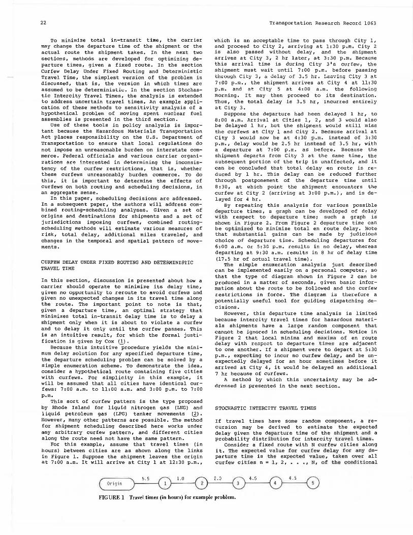
For this example, assume that travel times (in hours) between cities are as shown along the links in Figure 1. Suppose the shipment leaves the origin at 7:00 a.m. It will arrive at City 1 at 12:30 p.m.,

Origin

Transportation Research Record 1063

which is an acceptable time to pass through City 1, and proceed to City 2, arriving at 1:30 p.m. City 2 is also passed without delay, and the shipment arrives at City 3, 2 hr later, at 3:30 p.m. Because this arrival time is during City 3's curfew, the shipment must wait until 7:00 p.m. before passing th~ough City 3, a delay of :J.5 hr. Leaving City 3 at 7:00 p.m., the shipment arrives at City 4 at 11:30 p . m. and at City 5 at 4:00 a.m. the following morning. It may then proceed to its destination. Thus, the total delay is 3. 5 hr, incurred entirely at City 3.

Suppose the departure had been delayed 1 hr, to 8:00 a.m. Arrival at Cities 1, 2, and 3 would also be delayed 1 hr, but the shipment would still miss the curfews at City 1 and City 2. Because arrival at City 3 would now be at 4:30 p.m. instead of 3:30 p.m., delay would be 2.5 hr instead of 3.5 hr, with a departure at 7:00 p.m. as before. Because the shipment departs from City 3 at the same time, the subsequent portion of the trip is unaffected, and it can be concluded that total delay en route is re­duced by 1 hr. This delay can be reduced further through postponement of the departure time until 8:30, at which point the shipment encounters the curfew at City 2 (arriving at 3:00 p.m.), and is de­layed for 4 hr.

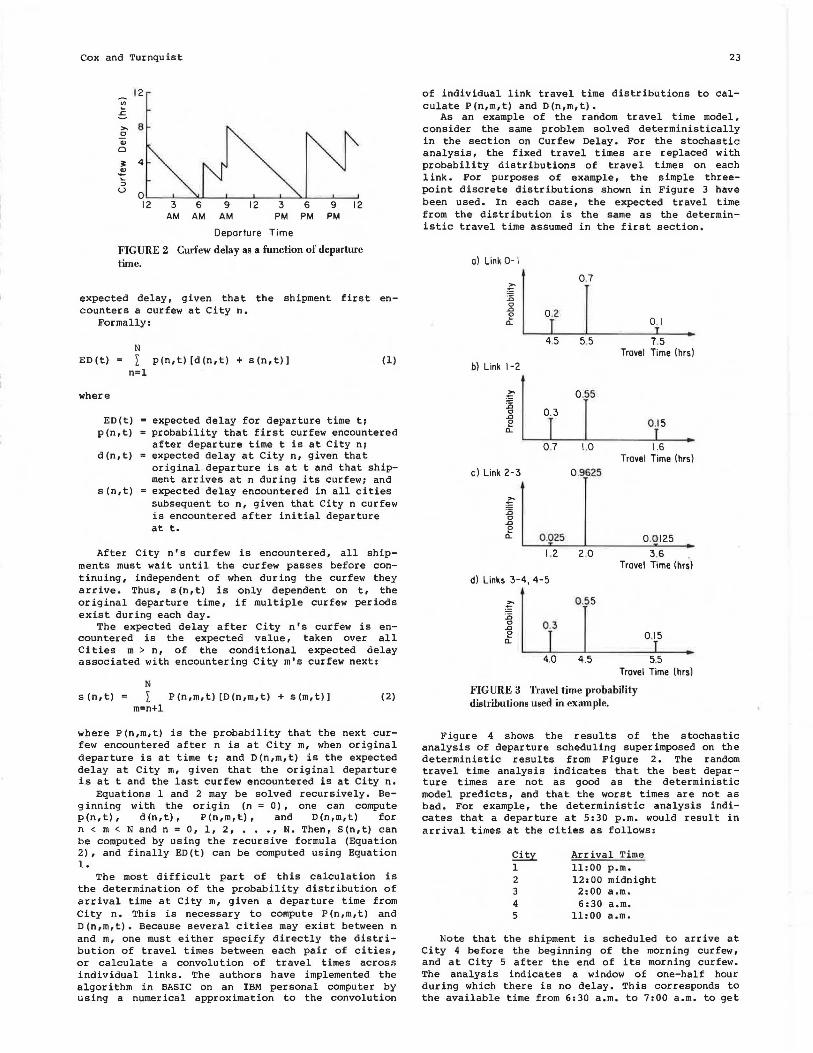
By repeating this analysis for various possible departure times, a graph can be developed of delay with respect to departure time; such a graph is shown in Figure 2. From Figure 2 departure time can be optimized to minimize total en route delay. Note that substantial gains can be made by judicious choice of departure time. Scheduling departures for 6:00 a.m. or 5:30 p.m. results in no delay, whereas departing at 9:30 a.m. results in 8 hr of delay time (17.5 hr of actual travel time).

The simple enumeration analysis just described can be implemented easily on a personal computer, so that the type of diagram shown in Figure 2 can be produced in a matter of seconds, given basic infor­mation about the route to be followed and the curfew restrictions in force. The diagram is therefore a potentially useful tool for guiding dispatching de­cisions.

However, this departure time analysis is limited because intercity travel times for hazardous materi­als shipments have a large random component that cannot be ignored in scheduling decisions. Notice in Figure 2 that local minima and maxima of en route delal'~ with respect to departure times are adjacent to one another. If a shipment were to depart at 5:30 p.m., expecting to incur no curfew delay, and be un­expectedly delayed for an hour sometimes before it arrived at City 4, it would be delayed an additional 7 hr because of curfews.

A method by which this uncertainty may be ad­dressed is presented in the next section.

STOCHASTIC INTERCITY TRAVEL TIMES

If travel times have some random component, a re­cursion may be derived to estimate the expected delay given the departure time of the shipment and a probability distribution for intercity travel times.

Consider a fixed route with N curfew cities along it. The expected value for curfew delay for any de­parture time is the expected value, taken over all curfew cities n = 1, 2, ••• , N, of the conditional

FIGURE 1 Travel times (in hours) for example problem.

Cox and Turnquist

12

"' 5 >. e 0

"' 0

;i: 4 ~ :; u

3 6 9 12 3 6 9 12 AM AM AM PM PM PM

Departure Time

FIGURE 2 Curfew delay as a function of departure time.

expected delay, given that the shipment first en­counters a curfew at City n.

Formally:

N ED(t) • L p(n,t)[d(n,t) + s(n,t)]

n= l (1)

where

ED(t) p(n,t)

d (n,t)

s (n,t)

expected delay for departure time ti probability that first curfew encountered after departure time t is at City n1 expected delay at City n, given that original departure is at t and that ship­ment arrives at n during its curfew; and expected delay encountered in all cities subsequent to n, given that City n curfew is encountered after initial departure at t.

After City n's curfew is encountered, all ship­ments must wait until the curfew passes before con­tinuing, independent of when during the curfew they arrive. Thus, s (n,t) is only dependent on t, the original departure time, if multiple curfew periods exist during each day.

The expected delay after City n's curfew is en­countered is the expected value, taken over all Cities m > n, of the conditional expected delay associated with encountering City m's curfew next:

N

s (n,t) = L P(n,m,t) [D(n,m,t) + s (m,t) I (2) m=n+l

where P(n,m,t) is the probability that the next cur­few encountered after n is at City m, when original departure is at time t; and D(n,m,t) is the expected delay at City m, given that the original departure is at t and the last curfew encountered is at City n.

Equations 1 and 2 may be solved recursively. Be­g inning with the origin (n = 0), one can compute p(n,t), d(n,t), P(n,m,t), and D(n,m,t) for n < m < N and n = O, 1, 2, ••• , N. Then, S(n,t) can be computed by using the recursive formula (Equation 2), and finally ED(t) can be computed using Equation 1.

The most difficult part of this calculation is the determination of the probability distribution of arrival time at City m, given a departure time from City n. This is necessary to compute P(n,m,t) and D(n,m,t). Because several cities may exist between n and m, one must either specify directly the distri­bution of travel times between each pair of cities, or calculate a convolution of travel times across individual links. The authors have implemented the algorithm in BASIC on an IBM personal computer by using a numerical approximation to the convolution

23

of individual link travel time distributions to cal­culate P(n,m,t) and D(n,m,t).

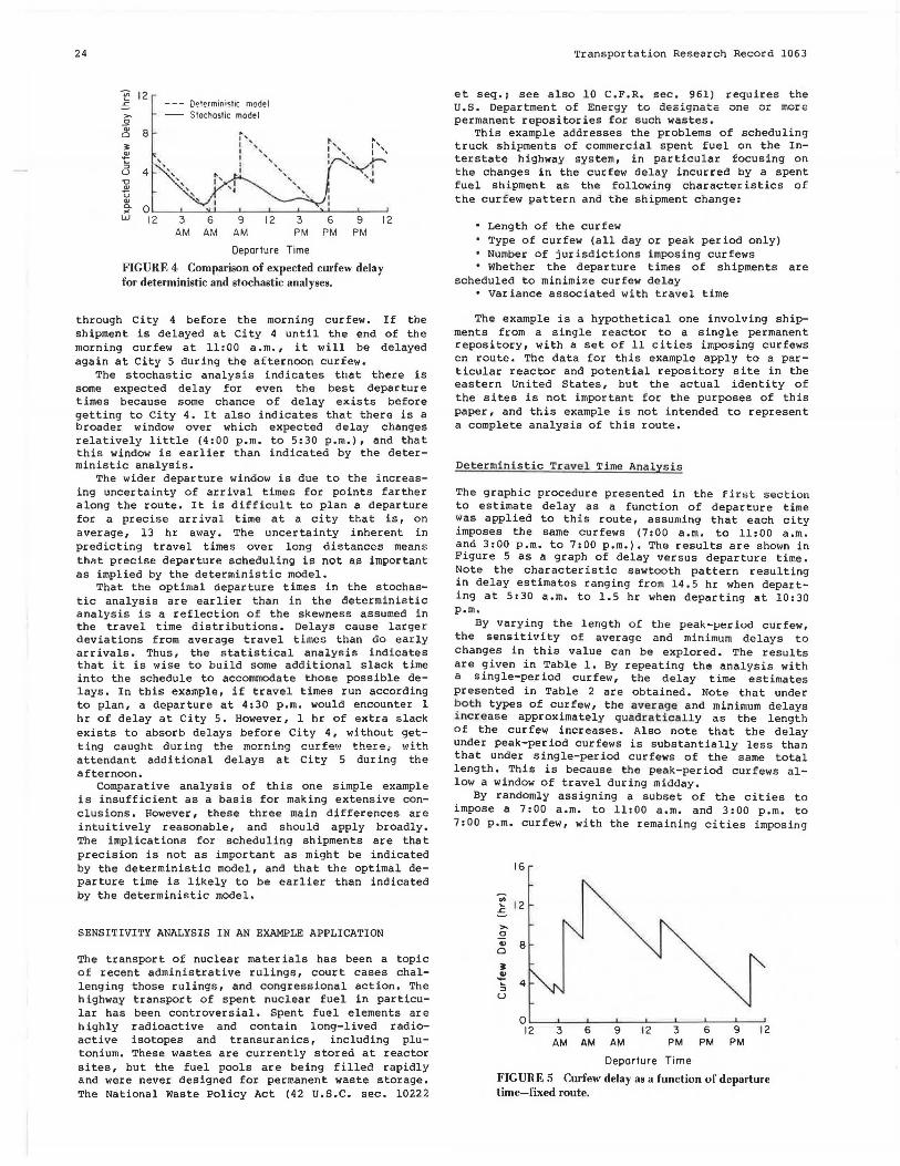
As an example of the random travel time model, consider the same problem solved deterministically in the section on Curfew Delay. For the stochastic analysis, the fixed travel times are replaced with probability distributions of travel times on each link. For purposes of example, the simple three­point discrete distributions shown in Figure 3 have been used. In each case, the expected travel time from the distribution is the same as the determin­istic travel time assumed in the first section.

al Link 0-1

0.2

I 4.5

bl Link 1-2

£

1 :.0

0.3 0

"" I e a..

0.7

cl Link 2-3

£ :.0 0

"" 0

it 0.025 T

1.2

d) Links 3-4, 4-5

£

1

:.0 0 0.3 "" e I a..

4.0

0 .7

l 5.5

0 .55

I 1.0

0.9625

I 2.0

0.55

I 4.5

0 .1 I

7.5 Travel Time (hrs)

0.1 5 I 1.6 •

Travel Time (hrs)

0.0 125 - . 3.6 '

Travel Time (hr~)

0.15 I ..

5.5 Travel Time (hrs)

FIGURE 3 Travel time probability distributions used in example.

Figure 4 shows the results of the stochastic analysis of departure scheduling superimposed on the deterministic results from Figure 2. The random travel time analysis indicates that the best depar­ture times are not as good as the deterministic model predicts, and that the worst times are not as bad. For example, the deterministic analysis indi­cates that a departure at 5:30 p.m. would result in arrival times at the cities as follows:

City Arrival Time 1 11:00 p.m. 2 12:00 midnight 3 2:00 a.m. 4 6:30 a.m. 5 11:00 a.m.

Note that the shipment is scheduled to arrive at City 4 before the beginning of the morning curfew, and at City 5 after the end of its morning curfew. The analysis indicates a window of one-half hour during which there is no delay. This corresponds to the available time from 6:30 a.m. to 7:00 a.m. to get

24

~ 12

=-,,.. 0

~ 8 3:

~ c3 4

"" ~ u

"'

Determini•tic model Slochostic model . ,,

I ', I ' I '

'

~ o .._~-'-~-"-'--~'--~-'-~---'-~~'--~-'-~-' w 12 3

AM 6 9

AM AM 12 3

PM

Departure Time

6 PM

9 12 PM

FIGURE 4 Comparison of expected curfew delay for deterministic and stochastic analyses.

through City 4 before the morning curfew. If the shipment is delayed at City 4 until the end of the morning curfew at 11:00 a.m., it will be delayed again at City 5 during the afternoon curfew.

The stochastic analysis indicates that there is some expected delay for even the best departure times because some chance of delay exists before getting to City 4. It also indicates that there is a b roader window over which expected delay changes relatively little (4:00 p.m. to 5:30 p.m.), and that this window is earlier than indicated by the deter­ministic analysis.

The wider departure window is due to the increas­ing uncertainty of arrival times for points farthe r along the route. It is difficult to plan a departure for a precise arrival time at a city that is, on average, 13 hr away. The uncertainty inherent in predicting travel times over long distances means thnt precise departure scheduling is not as important as implied by the deterministic model.

That the optimal departure times in the stochas­tic analysis are earlier than in the deterministic analysis is a reflection of the skewness assumed in the travel time distributions. Delays cause larger deviations from average travel times than do early arrivals. Thus, the statistical analysis indicates that it is wise to build some additional slack time into the schedule to accommodate those possible de­lays. In this example, if travel times run according to plan, a departure at 4:30 p.m. would encounter 1 hr of delay at City 5. However, 1 hr of extra slack exists to absorb delays before City 4, without get­t i ng caught during the morn i ng curfew there, with attendant additional delays at City 5 during the afternoon.

Comparative analysis of this one simple example is insufficient as a basis for making extensive con­clus i ons. However, these three main differences are intuitively reasonable, and should apply broadly. The implications for scheduling shipments are that precision is not as important as might be indicated by the deterministic model, and that the optimal de­parture time is likely to be earlier than indicated by the deterministic model.

SENSITIVITY ANALYSIS IN AN EXAMPLE APPLICATION

The transport of nuclear materials has been a topic of recent administrative rulings, court cases chal­lenging those rulings, and congressional action. The highway transport of spent nuclear fuel in particu­lar has been controversial. Spent fuel elements are highly radioactive and contain long-lived radio­active isotopes and transuranics, including plu­tonium. These wastes are currently stored at reactor sites, but the fuel pools are being filled rapidly and were never designed for permanent waste storage. The National waste Policy Act (42 u.s.c. sec. 10222

Transportation Research Record 1063

et seq.; see also 10 C.F.R. sec. 961) requires the U.S. Department of Energy to designate one or more permanent repositories for such wastes.

This example addresses t he problems of scheduling truck shipments of commercial spent fuel on the In­terstate highway system, in particular focusing on the changes in the curfew delay incurred by a spent fuel shipment as the following characteristics of the curfew pattern and t he shipment change:

• Length of the curfew • Type of curfew (all day or peak period only) • Number of jurisdictions imposing curfews • Whether the departure times of shipments are

scheduled to minimize curfew delay • Variance associated with travel time

The example is a hypothetical one involving ship­ments from a single reactor to a single permanent repository, with a set of 11 cities imposing curfews e n route . The data for thi s example apply to a par­ticular reactor and potential repository site in the eastern United States, but the actual identity of the sites is not important for the purposes of this paper, and this example is not intended to represent a complete analysis of this route.

Determin i stic Tr.avel Time Analysis

The graphic procedure presented in the firs t sec t i on to estimate delay as a function of departure time was applied to this route, assuming that each city imposes the same curfews (7:00 a.m. to 11:00 a.m. and 3:00 p.m. to 7:00 p.m.) . The results are shown in Figure 5 as a graph of delay versus departure time. Note the characteristic sawtooth pattern resulting in delay estimates ranging from 14.5 hr when depart­ing at 5130 a.m. to 1.5 hr when departing at 10:30 p.m.

By varying the length of the peak-period curfew, the sensitivity of average and minimum delays to changes in this value can be explored. The results are given in Table 1. By repeating the analysis with a single-period curfew, the delay time estimates presented in Table 2 are obtained. Note that under ~oth types of curfew, the average and minimum delays l.ncrease approximately quadratically as the length Of the curfew increases. Also note that the delay under peak-period curfews is substantiallv less than that under single-period curfews of the - same total length. This is because the peak-period curfews al­low a window of travel during midday.

By randomly assigning a subset of the cities to impose a 7:00 a.m. to 11 : 00 a . m. and 3 : 00 p.m. to 7:00 p.m. curfew, with the remaining cities imposing

~ .<:::

>-E

"' 0

):

-t :::J u

16

12

8

4

3 6 9 AM AM AM

12 3 6 9 12 PM PM PM

Departure Time

FIGURE 5 Curfew delay as a function of departure time-fixed route.

Cox and Turnquist

TABLE I Length of Peak-Period Curfew Versus Average and Minimum Delays

Average Delay over All Departure Times

Curfew Period (hr)

6:00 a.m.-11:00 a.m. 3:00 p.m.-8:00 p.m. 12

7:00 a.m.-11:00 a.m. 3:00 p.m.-7:00 p.m. 7.7

7:00 a.m.-10:00 a.m. 3:30 p.m.-6:30 p.m. 4.0

7:00 a.m.-9:00 a.m. 4:00 p.m.-6:00 p. m. 2.0

7: 30 a.m.-8: 30 a.m. 4:30 p.m.-5:30 p.m. 0.4

TABLE 2 Single-Period Curfew Analysis

Curfew Period

6:00 a.m.-8:00 p.m. 7:00 a.m.-7:00 p.m. 8:00 a.m.-6:00 p.m. 9:00 a.m.-5:00 p.m.

10:00 a.m.-4:00 p.m. 3:00 p.m.-7:00 p.m. 4:00 p.m.-6:00 p.m.

Average Delay over All Departure Times (hr)

28.3 22.6 13 10.8

5.9 2.9 I.I

Minimum Delay over All Departure Times (hr)

4.5

l.5

l.O

0

0

Minimum Delay over All Departure Times (hr)

16.5 14.5 5.0 3.0 l.O 0 0

no curfew, one can estimate how delay varies with the number of cities imposing curfews on the route. The results are shown in Figure 6. On this scatter­plot, each point r~presents the average curfew delay with a random subset of cities imposing curfews on the route where the number of cities in the subset is plotted on the x-axis. Note that the relationship between delay and the number of cities with curfews is approximately linear. However, for any g~ven num­ber of cities imposing a curfew, the variance in total shipment delay is large, indicating that the total delay is sensitive to which cities impose cur­fews.

8

• ~ .

I a .i:::;

§ I 6 "" ~ I .2 . 0 A ft ., 6

I I 0 § . I ~ A I

8 A

~ 4

I • .

I 2 • :J u

I I .

9 &

"' 6 Cl' . E? 3

. & 6 . 8 ., a I •

~ t

0 0 2 4 6 8 10 12

Number of Cities Imposing Curfews

FIGURE 6 Delay versus number of cities imposing curfews.

25

Results for Stochastic Travel Times

To compute the delay under stochastic travel times, the recursion formulas discussed in the section on Stochastic Intercity Travel Times were used. Assuming a curfew of 7:00 a.m. to 11:00 a.m. and 3:00 p.m. to 7:00 p.m. for all cities, Figure 7 shows delay as a function of departure time for three different values of intercity travel time variance. The first point

16

14

12

"' .c 10

"" .2 "' 8

0

~ 6 .!!! ~

:J 4 u

2

0 12 3 6 9

AM AM AM 12

Zero variance Low variance High variance

3 6 9 PM PM PM

Departure Time

FIGURE 7 Curfew delay profile as variance of travel time changes.

12

to note is that for the zero-variance case, the delay function is the same as the one shown in Figure 5, as expected. Second, note that as the variance in­creases, the difference between minimum and maximum delay is reduced, and the profile becomes smoother. This is to be expected; as travel times grow more uncertain, it becomes less likely that either the best possible outcome (minimum delay) or worst pos­sible outcome (maximum delay) will be observed. Thus, the expected delay becomes less sensitive to the actual departure time of the shipment. Last, note that the local minima of the delay profile move to the left as variance increases. As variance in­creases, it is more likely that a shipment wil,J. be delayed unexpectedly. If a shipment departed during the zero-variance delay minimum, such as at 10: 3 0 p .m., a good chance exists that the actual delay would be as though it left at 11:00 p.m., which is a local maxima, because it is more likely that travel time will be longer than expected rather than less than expected. It is wiser, in the case of uncertain travel times, to depart earlier to account for the expected values of delays. Thus, the minima for scheduling departure times should move to the left •

SUMMARY

In the first section on Curfew Delay, it was argued that the natural approach to delaying a shipment along a route in the face of curfews was the optimal strategy to minimize total curfew delay. As a re­sult , given a departure time and i .ntercity travel t imes , the delay t ime may be estimated using a simpl.e enumeration . In the section on Stochastic In­tercity Travel Times, a recursive procedure was pre­sented for estimating expected delay, given a depar­ture time, for random travel times .

The major implications of uncertain travel times in the analysis are as follows:

26

1. It is unreasonable to expect delays as small as those indicated by optimal deterministic solu­tions;

2. As uncertainty in travel times increases, the relative advantages of precise dispatching decrease;

3. The optimal departure time when travel times are uncertain is earlier than when they are assumed to be known with certainty.

The important benefits from the models described in this paper are that they are relatively simple; require modest amounts of data; can be operated eas­ily on a personal computer 1 and can provide esti­mates of how much delay can be expected, how impor­tant precise departure scheduling is, and what are the best departure times in a given situation,

In the third section, a hypothetical example was presented of spent nuclear fuel shipments between one specific reactor and a single potential perma­nent spent fuel repository. The purpose of this ex-

Transportation Research Record 1063

ample is to demonstrate how the models developed in this paper can be used t o do sensitivity analysis on various elements of hazardous materials routing­scheduling problems. It should not be construed as a complete analysis of the effects of curfews on haz­ardniJ'O m"t<>ria l s movement. The authors believe, how­ever, that it does demonstrate the usefulness of these analytic tools in addressing several important issues in hazardous materials transportation.

REFERENCES

1. R.G. Cox. Routing and Scheduling of Hazardous Materials Shipments: Algorithmic Approaches to Managing Spent Nuclear Fuel Transport. Ph.D. dissertation. Cornell University, Ithaca, N.Y., 1984.

2. National Tank Truck Carr i ers v. Burke, 608 F2d 819 (1979), 535 F.Supp. 509 (1982).