Embed Size (px)
Citation preview

Scheduling:Overview of Concepts and Methods
Amgen
March 30, 2005
Bill Wolfe, CSUCI


Scheduling: Definition
• Assigning resources to activities over time• Satisfy constraints
– feasible schedules
• Create “good” schedules– criteria/objective

Scheduling
• Activities: job, task, delivery, transportation, machining, milling, grinding, painting, sanding, chemical bath, ..
• Resources: machines, operators, power, etc.• Constraints: capacity, precedence, cost, due dates,
nonpreemptive, power, size/shape, union rules, ..• Criteria: profit/cost, priorities, preferences, make
span, utilization, customer satisfaction, opportunity, ..

Example Domains
• Universities• Satellites• Factories• Transportation• Traffic• Home Construction• Military Logistics
• Vehicle Routing• Facility Maintenance• Sports Leagues• Courts• Hospitals• etc.• etc.

Factory Scheduling
• Activities:
• Resources:
• Constraints:
• Objectives:

Satellite Scheduling
• Activities:
• Resources:
• Constraints:
• Objectives:

University Scheduling
• Activities:
• Resources:
• Constraints:
• Objectives:

Scheduling is difficult
• Modeling: real-world domains are hard to model.
• Complexity: large # options, combin. explosion, NP.
• Criteria/Objectives: vague, ambiguous, difficult to quantify, multiple objectives, conflicting objectives.
• Uncertainty: unexpected events, new orders, cancellations, changing costs/priorities, failures, ..
• Domain-Specific Dependencies: unique heuristics and rules of thumb -- makes it hard to transfer results from one domain to another.

Example: Distribution Criteria
• Different types of:– Customers– Priorities– Tasks
• Might want the resulting schedule to satisfy distribution of job types:– 50 % Type A, 25% Type B, 25% Type C
• Might want the resulting schedule to have:– 100% of type A jobs (i.e.: all type A jobs make the schedule)– 100% of priority 10 jobs (i.e.: all the jobs with the top priority
make the schedule.

Multiple Conflicting Criteria
• Request:– High quality product– On time– Low cost
• Response:– Pick any two!

Levels of Scheduling (Morten)
• Long Range Planning– Plant expansion, layout, design
• Middle Range Planning– Production smoothing, logistics
• Short Range Planning– Requirements, shop bidding, due date setting
• Scheduling– Shop routing, line balancing, batch sizing
• Reactive Scheduling– Hot jobs, down machines, late material

Approaches to Scheduling
• Manual
• OR/Mathematical/Exact
• Heuristic Search
• Advanced Algorithms
• Expert Systems & AI
• Mix
• Scheduling “System”

OR Methods
• Mathematical Programming– Linear/nonlinear programming
– Dynamic, programming
– Integer/mixed programming
– Network Analysis
• Probabilistic Modeling– Inventory Theory
– Queuing Theory
– Markov Chains

Heuristic Methods
• Generate schedules that are “good enough”• Constructive vs. Repair• Search
– Limited depth/breath first search– Look ahead methods, A*– Neighborhood search, Hill Climbing
• Bottleneck-driven, Constraint-driven• Min-Conflicts• Priority Dispatch
– Priority sort, resource allocation rules• Task assignment rules
– Rules for resource allocation, conflict resolution, bump

Advanced Methods
• Genetic Algorithms• Neural Networks• Simulated Annealing
– Exploitation vs. Exploration
– Intensification vs. Diversification
• Expert Systems• Fuzzy Systems• Mixes of any/all methods
Desirable Algorithm Attributes
• Fast
• Accurate– Produces high quality schedules
• Simple– Easy to understand– Operators, users, customers

Classic Problems
• Linear Programming– Resources, activities, constraints.– Linear constraints/objective function
• Transportation Problem• Assignment Problem• Maximum Flow• Shortest Paths in Weighted Graphs• Knapsack• Traveling Salesman• Weighted Shortest Processing Time• Weighted Early-Tardy Processing Time• PERT-CPM

Example: Knapsack Problem
• Knapsack– n items with weight wi and value vi.
– Constraint: wi <= w
– Maximize: vi
• Example:– Set of projects pi with cost ci and value vi
– Constraint: ci <= c
– Maximize: vi

Example: Activity Selection
• n activities– start time = si
– stop time = fi
• Select the maximum number of non-overlapping activities
• Optimal solution: – Greedy algorithm:
• sort by finish time: f1<= f2 <= ..... <= fn
• allocate and remove conflicting activities.

Time
Competing Activities
Resource:

Assignment Problem
• Let cij = cost of assigning resourcei to taskj
• Find xij that minimizes: i j cij xij
• Constraints: j xij = 1 for all i
• every resource has one task.
i xij = 1 for all j• every task has one resource.
– xij = 0 or 1 (the decision variable)• permutation matrix
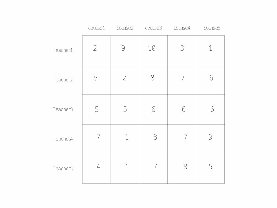
course1 course2 course3 course4 course5
Teacher1
Teacher2
Teacher3
Teacher4
Teacher5
2 9 10 3 1
5 2 8 7 6
5 5 6 6 6
7 1 8 7 9
4 1 7 8 5

Transportation Problem
• Probably the most important special case of linear programming.
• Source i supplies si units.• Destination j has demand for dj units.• Let cij denote the cost per unit distributed.• Let xij denote the number of units distributed from source i to
destination j.• Minimize: i j cij xij
• Constraints: j xij = si
i xij = dj
– xij >= 0.

Traveling Salesman Problem
• Classic problem, NP-Complete.• Find the shortest closed path through a set of “cities”.
– visit each city once and only once.– return to the start city.
• Heuristics:– nearest city (constructive)– 2-opt (improvement/hill climbing)– neural networks (Hopfield)– genetic algorithms– etc.


System Approach
• Human operators
• Tools for managing complexity, uncertainty
• GUI, visualization techniques
• Domain Specific support– Information Systems/Database support– Decision/Advisory support
• Communications/messaging


Dynamic Environments
• Scheduling in a rapidly changing environment can be an exercise in futility.
Uncertainty
Task Complexity
real-time control
easy
hard
ripe

Uncertainty vs. Task Complexity
Uncertainty
Task Complexity
real-time control
easy
hard
ripe

Nervous Scheduling
• Refining a schedule in response to “noise” can lead to nervous scheduling– Lots of changes in a short time– Confused operators, customers– Overreaction to meaningless differences
• “Noise” comes from modeling inaccuracies, and poor estimates of scheduling criteria.
• Noisy environments control systems.

Example: Thermostat
72
73
71
Time
Temperature
(Set)

No Scheduling System is an Island
• Scheduling systems interact with, and depend on, other systems, both inside and outside the plant.
• Changes become more costly as time progresses.• Priority Aging: when a task is “put on the
schedule”, it creates expectations and spawns related subtasks (i.e.: grows “roots”), making it more and more costly to cancel as time goes on.

Progressive Refinement
• Outday (e.g.: a month out)– Most important/costly
constraints considered– Constraints may be violated
(e.g.: Overbooking)– Allow new tasks, cancellations– Get supplier commitments
• Stabilization (e.g.: a week out)– Most hard constraints satisfied– Check intersystem
commitments– Look for schedule
improvements– Cancellations are now costly
• Near real time (e.g.: a day out)
– All hard constraints satisfied.
– Look for last minute opportunities
• Real time– Implementation
– Safety checks
– Monitoring operations
– Data collection

Hard vs. Soft Constraints
• Hard rigid, unbending– Must be satisfied– Define the search space
• Soft pliable, flexible, relaxable– Measured in degrees– Define the quality of a schedule
• Feasible schedule:– Satisfies all hard constraints
• Optimal schedule:– Feasible, and has best possible score on soft constraints

Window of Opportunity
• Period of time (t0, tf) when a task can be done
– Hard constraint: must be inside the window
– Soft constraint: middle of the window is best
t0 tf
Utility Function
t
Task
score


General Rule of ThumbTask Value
Task Laxity
First
Last
Low Laxity, High Value, tasks shouldbe scheduled first.
High Laxity, Low Value, tasks shouldbe scheduled last.

Another Rule of Thumb
• Schedule the shorter, higher value, jobs as soon as possible.
• Applies primarily to highly uncertain environments.
• A complex schedule has little chance of success in a highly uncertain environment.– so, get the easy, high value, jobs done as soon
as they pop up.
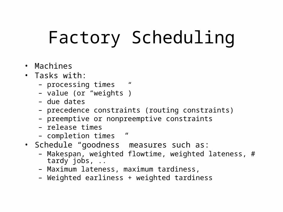
Factory Scheduling
• Machines• Tasks with:
– processing times– value (or “weights”)– due dates– precedence constraints (routing constraints)– preemptive or nonpreemptive constraints– release times– completion times
• Schedule “goodness” measures such as:– Makespan, weighted flowtime, weighted lateness, # tardy jobs, ..– Maximum lateness, maximum tardiness, – Weighted earliness + weighted tardiness

Weighted Shortest Processing Time
• n jobs, single machine• pi = processing time for job i• wi = weight (or value) of job i• Objective: Minimize:
– weighted flow time: wi (Ci – ri)– weighted completion time: wi Ci
– weighted lateness: wi (Ci – di)• Optimal ordering of jobs is:
w1/p1 >= w2/p2 >= .........>=wn/pn • “Importance per unit time”

WSPT Example
• 3 jobs: – job1: worth $1000, takes 50 hours– job2: worth $200, takes 5 hours– job3: worth $2000, takes 120 hours
• Sort by:– job1: priority = $20.00/hr.– job2: priority = $40.00/hr.– job3: priority = $16.67/hr.
• Solution: job2 job1 job3

WSPT Example 2
• n jobs:– jobi has processing time pi
– jobi has due date d (same due date for all jobs)
– jobi has weight 1 (equal value jobs)
• Minimize the number of late jobs.
• Solution:– order by 1/pi shortest jobs first.

Weighted Early-Tardy Problem
• Jobs with due dates and weights• Penalty for being late (wT)• Penalty for being early (wE)• NP hard
Due date
Earlinesspenalty
Latenesspenalty
Task
Slope = wE
Slope = wT
Time

References
• Heuristic Scheduling Systems– T. E. Morton, D. W. Pentico, Wiley, 1993.– ISBN: 0471578193.
• Intelligent Scheduling– M. Zweben, M. Fox. Morgan Kaufmann, 1998. – ISBN: 1558602607
• Introduction to Algorithms– T. H. Cormen, C. E. Leiserson, R. L. Rivest, C. Stein– The MIT Press; 2nd edition, 2001.– ISBN: 0262032937
• Introduction to Operations Research– F. Hiller, G. Lieberman– McGraw-Hill Science/Engineering/Math; 7 edition, 2002.– ISBN: 0072535105