SCHEDULING MIXED-CRITICALITYREAL-TIME SYSTEMS

Haohan Li

A dissertation submitted to the faculty of the University of North Carolina at ChapelHill in partial fulfillment of the requirements for the degree of Doctor of Philosophyin the Department of Computer Science.

Chapel Hill2013

Approved by:

Sanjoy K. Baruah

James H. Anderson

Kevin Jeffay

Montek Singh

Leen Stougie

©2013Haohan Li

ALL RIGHTS RESERVED

ii

ABSTRACT

HAOHAN LI: Scheduling Mixed-Criticality Real-Time Systems(Under the direction of Dr. Sanjoy K. Baruah)

This dissertation addresses the following question to the design of scheduling policies and

resource allocation mechanisms in contemporary embedded systems that are implemented

on integrated computing platforms: in a multitasking system where it is hard to estimate a

task’s worst-case execution time, how do we assign task priorities so that 1) the safety-critical

tasks are asserted to be completed within a specified length of time, and 2) the non-critical

tasks are also guaranteed to be completed within a predictable length of time if no task is

actually consuming time at the worst case?

This dissertation tries to answer this question based on the mixed-criticality real-

time system model, which defines multiple worst-case execution scenarios, and demands a

scheduling policy to provide provable timing guarantees to each level of critical tasks with

respect to each type of scenario. Two scheduling algorithms are proposed to serve this

model. The OCBP algorithm is aimed at discrete one-shot tasks with an arbitrary number

of criticality levels. The EDF-VD algorithm is aimed at recurrent tasks with two criticality

levels (safety-critical and non-critical). Both algorithms are proved to optimally minimize

the percentage of computational resource waste within two criticality levels. More in-depth

investigations to the relationship among the computational resource requirement of different

criticality levels are also provided for both algorithms.

iii

Dedicated to my fiancee and my parents.

iv

ACKNOWLEDGEMENTS

I have always been feeling lucky when I pursue the doctoral degree at The University of

North Carolina at Chapel Hill, because I have received too much help and support to repay.

The first and the most important of all, the best part of my graduate student life is to have

Sanjoy Baruah as my advisor. He shows me how attractive the computer science research

is, how kind a teacher can be, and how wonderful an academic life will be. It wouldn’t be

possible for me to become who I am without him, and it is my dream to become who he is.

I would like to express my sincerest appreciation to my committee members: Jim

Anderson, Kevin Jeffay, Montek Singh, and Leen Stougie, for the time and energy they

spend on my dissertation. It is my great fortune to receive guidance and advices from them

during my work. I am also very grateful to my co-authors: Vincenzo Bonifaci, Gianlorenzo

D’Angelo, Alberto Marchetti-Spaccamela, Nicole Megow, Suzanne Van Der Ster, Bipasa

Chattopadhyay, and Insik Shin. It is my honor and my pleasure to work with so many great

minds on numerous interesting problems.

I want to thank all my friends in the real-time systems group, from whom I learn a lot:

Cong Liu, Mac Mollison, Glenn Elliott, Zhishan Guo, Jeremy Erickson, Bryan Ward, Alex

Mills, Andrea Bastoni, Hennadiy Leontyev and Bjorn Brandenburg. The delightful memory

in this great group will never fade away.

I am extremely proud to spend five years in The Department of Computer Science

at UNC. I am grateful to the department for awarding me the Computer Science Alumni

Fellowship that supports my dissertation writing. Also, I appreciate the infinite help from

all the faculty members and staffs. Especially, I would like to say thanks to Jodie Turnbull

for her splendid service and unreserved help during my study and job hunting.

I wish to say “thank you” to my parents, for their constant and unconditional love.

v

Finally, I am deeply thankful to my fiancee Zhongwan for her love, support, trust,

passion, and inspiration. Thank you for meeting me; thank you for loving me; thank you for

saying “yes”. I wish to have my happily ever after with you.

vi

TABLE OF CONTENTS

LIST OF TABLES . . . . . . . . . . . . . . . . . . . . . . . . . . . . . . . . . . . . . . . . . . . . . . . . . . . . . . . . . . . . . . . . . . ix

LIST OF FIGURES. . . . . . . . . . . . . . . . . . . . . . . . . . . . . . . . . . . . . . . . . . . . . . . . . . . . . . . . . . . . . . . . . x

LIST OF ABBREVIATIONS . . . . . . . . . . . . . . . . . . . . . . . . . . . . . . . . . . . . . . . . . . . . . . . . . . . . . . . xi

1 Introduction . . . . . . . . . . . . . . . . . . . . . . . . . . . . . . . . . . . . . . . . . . . . . . . . . . . . . . . . . . . . . . . . . . . . . 1

1.1 Overview of Real-Time Systems . . . . . . . . . . . . . . . . . . . . . . . . . . . . . . . . . . . . . . . . . . . . 1

1.2 Motivation . . . . . . . . . . . . . . . . . . . . . . . . . . . . . . . . . . . . . . . . . . . . . . . . . . . . . . . . . . . . . . . . . 3

1.3 Models for Real-Time Systems and Mixed-Criticality Systems . . . . . . . . . . . . . . . 4

1.3.1 Real-time Jobs and Recurrent Tasks . . . . . . . . . . . . . . . . . . . . . . . . . . . . . . . . . 4

1.3.2 Overview of Mixed-Criticality Systems . . . . . . . . . . . . . . . . . . . . . . . . . . . . . . . 7

1.3.3 Mixed-Criticality Jobs . . . . . . . . . . . . . . . . . . . . . . . . . . . . . . . . . . . . . . . . . . . . . . . 9

1.3.4 Mixed-Criticality Recurrent Tasks . . . . . . . . . . . . . . . . . . . . . . . . . . . . . . . . . . . 13

1.4 Thesis Statement . . . . . . . . . . . . . . . . . . . . . . . . . . . . . . . . . . . . . . . . . . . . . . . . . . . . . . . . . . . 14

1.5 Contributions . . . . . . . . . . . . . . . . . . . . . . . . . . . . . . . . . . . . . . . . . . . . . . . . . . . . . . . . . . . . . . 15

2 Prior Work . . . . . . . . . . . . . . . . . . . . . . . . . . . . . . . . . . . . . . . . . . . . . . . . . . . . . . . . . . . . . . . . . . . . . . 18

2.1 Real-Time Scheduling Theory. . . . . . . . . . . . . . . . . . . . . . . . . . . . . . . . . . . . . . . . . . . . . . . 18

2.2 Mixed-Criticality Scheduling Theory . . . . . . . . . . . . . . . . . . . . . . . . . . . . . . . . . . . . . . . . 21

3 Scheduling Mixed-Criticality Jobs . . . . . . . . . . . . . . . . . . . . . . . . . . . . . . . . . . . . . . . . . . . . . . . . 26

3.1 Overview . . . . . . . . . . . . . . . . . . . . . . . . . . . . . . . . . . . . . . . . . . . . . . . . . . . . . . . . . . . . . . . . . . . 26

3.2 Worst-Case Reservation Scheduling . . . . . . . . . . . . . . . . . . . . . . . . . . . . . . . . . . . . . . . . . 27

3.3 Own-Criticality-Based-Priority Algorithm . . . . . . . . . . . . . . . . . . . . . . . . . . . . . . . . . . . 29

3.4 Load-Based OCBP Schedulability Test . . . . . . . . . . . . . . . . . . . . . . . . . . . . . . . . . . . . . . 31

vii

3.5 Speedup Factors of OCBP Algorithm . . . . . . . . . . . . . . . . . . . . . . . . . . . . . . . . . . . . . . . 38

3.6 Summary. . . . . . . . . . . . . . . . . . . . . . . . . . . . . . . . . . . . . . . . . . . . . . . . . . . . . . . . . . . . . . . . . . . 44

4 Scheduling Mixed-Criticality Implicit-Deadline Tasks . . . . . . . . . . . . . . . . . . . . . . . . . . . . . 46

4.1 An Overview of Algorithm EDF-VD . . . . . . . . . . . . . . . . . . . . . . . . . . . . . . . . . . . . . . . . 46

4.2 Schedulability Test: Pre-Runtime Processing . . . . . . . . . . . . . . . . . . . . . . . . . . . . . . . . 48

4.3 Run-time Scheduling Policy . . . . . . . . . . . . . . . . . . . . . . . . . . . . . . . . . . . . . . . . . . . . . . . . . 53

4.3.1 An Efficient Implementation of Run-Rime Dispatching . . . . . . . . . . . . . . . 54

4.4 Some Properties of EDF-VD Algorithm . . . . . . . . . . . . . . . . . . . . . . . . . . . . . . . . . . . . . 56

4.4.1 Comparison with Worst-Case Reservation Scheduling . . . . . . . . . . . . . . . . 56

4.4.2 Task Systems with U2(1)=0 . . . . . . . . . . . . . . . . . . . . . . . . . . . . . . . . . . . . . . . . . 58

4.5 Speedup Factor of EDF-VD Algorithm. . . . . . . . . . . . . . . . . . . . . . . . . . . . . . . . . . . . . . 59

4.6 Summary. . . . . . . . . . . . . . . . . . . . . . . . . . . . . . . . . . . . . . . . . . . . . . . . . . . . . . . . . . . . . . . . . . . 61

5 Scheduling Mixed-Criticality Arbitrary-Deadline Tasks . . . . . . . . . . . . . . . . . . . . . . . . . . . 63

5.1 Overview . . . . . . . . . . . . . . . . . . . . . . . . . . . . . . . . . . . . . . . . . . . . . . . . . . . . . . . . . . . . . . . . . . . 63

5.2 Schedulability Test . . . . . . . . . . . . . . . . . . . . . . . . . . . . . . . . . . . . . . . . . . . . . . . . . . . . . . . . . 65

5.3 Speedup Factor Result . . . . . . . . . . . . . . . . . . . . . . . . . . . . . . . . . . . . . . . . . . . . . . . . . . . . . . 71

5.4 Summary. . . . . . . . . . . . . . . . . . . . . . . . . . . . . . . . . . . . . . . . . . . . . . . . . . . . . . . . . . . . . . . . . . . 74

6 Other Contributions . . . . . . . . . . . . . . . . . . . . . . . . . . . . . . . . . . . . . . . . . . . . . . . . . . . . . . . . . . . . . 75

6.1 OCBP Algorithm on Mixed-Criticality Recurrent Tasks . . . . . . . . . . . . . . . . . . . . . 75

6.2 Multiprocessor Mixed-Criticality Scheduling . . . . . . . . . . . . . . . . . . . . . . . . . . . . . . . . 79

6.2.1 Global Mixed-Criticality Scheduling . . . . . . . . . . . . . . . . . . . . . . . . . . . . . . . . . 79

6.2.2 Partitioned Mixed-Criticality Scheduling . . . . . . . . . . . . . . . . . . . . . . . . . . . . . 84

7 Conclusion . . . . . . . . . . . . . . . . . . . . . . . . . . . . . . . . . . . . . . . . . . . . . . . . . . . . . . . . . . . . . . . . . . . . . . 86

7.1 A Summary of Research Results . . . . . . . . . . . . . . . . . . . . . . . . . . . . . . . . . . . . . . . . . . . . 86

7.2 Future Plan . . . . . . . . . . . . . . . . . . . . . . . . . . . . . . . . . . . . . . . . . . . . . . . . . . . . . . . . . . . . . . . . 88

BIBLIOGRAPHY. . . . . . . . . . . . . . . . . . . . . . . . . . . . . . . . . . . . . . . . . . . . . . . . . . . . . . . . . . . . . . . . . . . 90

viii

LIST OF TABLES

1.1 DO-178B Standard . . . . . . . . . . . . . . . . . . . . . . . . . . . . . . . . . . . . . . . . . . . . . . . . . . . . . . . . . 5

ix

LIST OF FIGURES

4.1 EDF-VD: The preprocessing phase. . . . . . . . . . . . . . . . . . . . . . . . . . . . . . . . . . . . . . . . . . 48

6.1 Global EDF-VD: The preprocessing phase. . . . . . . . . . . . . . . . . . . . . . . . . . . . . . . . . . . 83

x

LIST OF ABBREVIATIONS

CA Certification Authority

CM Criticality-Monotonic

EDF Earliest-Deadline-First

EDF-VD Earliest-Deadline-First with Virtual Deadlines

FAA Federal Aviation Administration

LCM Least Common Multiple

LHS Left-Hand Side

MC Mixed-Criticality

NP Non-deterministic Polynomial-time

OCBP Own-Criticality-Based-Priority

RTCA Radio Technical Commission for Aeronautics

SWaP Size, Weight and Power

UAV Unmanned Aerial Vehicle

WCET Worst-Case Execution Time

WCR Worst-Case Reservation

xi

CHAPTER 1

Introduction

Traditional real-time scheduling theory faces challenges in modern computation-intensive

and time-sensitive cyber-physical embedded systems. Nowadays, real-time embedded comput-

ing systems are widely used in safety-critical environments such as avionics and automobiles.

There are two conflicting trends in the development of these systems. One is that the safety

assurance requirements are increasingly emphasized. Some critical real-time tasks must

never fail to meet their deadlines, even under extremely harsh circumstances. The other

is that more functionalities are implemented on integrated platforms due to size, weight

and power (SWaP) constraints. Therefore, many non-critical real-time tasks will share

and compete for the computational resources with critical tasks. Unfortunately, traditional

real-time scheduling theory cannot provide a balance between these two requirements. The

existing techniques have to reserve unreasonably large amounts of computational resources

to ensure that every real-time task performs correctly under harsh circumstances — even

the non-critical ones. This inefficiency makes it desirable that the assumptions, abstractions

and objectives in traditional real-time scheduling theory be reconsidered, such that these

safety-critical systems will sacrifice neither reliability nor efficiency.

1.1 Overview of Real-Time Systems

Modern embedded systems broadly interact with physical environments, and commonly

require that every input signal is responded to within a predictable length of time. In these

systems, there are two notions of correctness, logical correctness and temporal correctness.

Logical correctness usually means “to generate the correct results”, which is quite commonly

required in general computing systems; temporal correctness usually means “to perform

actions at the required time”, which is an additional main objective in real-time systems.

Real-time systems are defined as systems that provide temporal correctness. In real-time

systems, the temporal predictability, which is often in the form of guaranteeing every task’s

response within strict deadlines, is as important as the performance (how fast an individual

task can complete) or the throughput (how many tasks can be completed over a long period

of time).

In real-time scheduling theory research, the scheduling algorithms that switch tasks and

allocate resources in real-time systems are studied. These algorithms are constructed based

on real-time task models. These models will be introduced in Section 1.3. These models

extract the essential information of the temporal behaviors of the tasks in a real-time system.

The scheduling algorithms must predictably assure a priori that all tasks are completed

by their deadlines, assuming that the tasks follow the specifications in the workload model.

Because these guarantees must be analytically proved before the actual execution of the

system, there are usually two types of algorithms on scheduling:

� Scheduling policies, sometimes called schedulers, are the algorithms that control the

run-time schedule. The scheduling policies will be executed along with real-time tasks,

and make scheduling decisions based on the time and/or the temporal behavior of

real-time tasks. Scheduling policies are generally required to be simple and fast because

they compete with real-time tasks and occupy computational resources.

� Schedulability tests are the algorithms that check before run-time if the deadlines are

guaranteed to be met. Schedulability tests can be complicated and time-consuming if

they can bring in better run-time performance and computational resource efficiency.

It is non-trivial to design schedulability tests, especially for real-time tasks with a

large variance of run-time behaviors because the tests must guarantee that no deadline

is missed in all possible system runs.

This dissertation focuses on a new real-time task model, the mixed-criticality task model.

Section 1.3 will describe the traditional model, the new model, and their differences. The

following chapters in this dissertation will introduce several scheduling algorithms aimed at

2

the mixed-criticality system model, while Section 1.5 gives an overview of all these scheduling

algorithms.

1.2 Motivation

The research of scheduling mixed-criticality systems starts from abstracting a realistic

problem — the certification requirement. Many safety-critical embedded systems must pass

certain safety certifications. In the certification processes, the certification authorities, such

as Federal Aviation Administration (FAA), will verify the safety standards within the system,

including the real-time constraints of the safety-critical tasks. It is important to note that

the certification authorities tend to be very conservative in the certification. They require

that the correctness be demonstrated under extremely rigorous and pessimistic assumptions,

which are very unlikely to occur in reality.

Traditional real-time scheduling techniques commonly do not work efficiently on these

certifiable systems. The reason is that the scheduling theory is based on abstract task

models. In these models, the tasks are usually specified by several parameters: the worst-

case execution time, the deadline and the release pattern. The objective is a scheduling

policy with a strong requirement: all deadlines must always be met. In order to fulfill this

requirement, the worst-case execution time (WCET) of a task, which is a parameter that

must be determined beforehand, is required never to be exceeded by the actual execution

time of this task. In practice, determining an exact WCET value for a task is very difficult

and remains an active area of research. Therefore, the WCET parameter used by the

certification authorities is typically a very conservative upper bound that highly exceeds

the true WCET. Moreover, in typical real-time system models, no isolation exists between

tasks in a traditional real-time system because all tasks are treated as equally important.

This implies a task will possibly miss its deadline if another task fails to be bounded by its

own WCET. As a result, in order to prevent any potential deadline miss, very pessimistic

WCET values must be used for all tasks in certifications. This will inevitably cause severe

computational resource waste. Past scheduling techniques that focus on meeting all deadlines

are not able to eliminate this waste.

3

Knowing the shortcomings of the traditional models, how do we abstract a certifiable

real-time system, and what kind of scheduling policies do we seek then? The key idea is to

observe that in many applications, the consequence of a deadline miss varies among tasks.

For example, in the RTCA DO-178B avionics software standard, as listed in Table 1.1,

the tasks are divided into five assurance levels, from level A to level E. In the standard, a

failure of a level-A task will have catastrophic results (e.g. causing a crash), while a failure

of a level-E task will have no influence on flight safety. Under these circumstances, it is

reasonable not to presuppose an objective that all low-criticality deadlines are always met.

Therefore, the mixed-criticality real-time system model is proposed by Vestal (Vestal, 2007)

on the basis of a new assumption that only high-criticality deadlines are guaranteed to be

met if high WCET estimations are used, and all deadlines are guaranteed to be met if low

WCET estimations are used. Under this new assumption, only high-criticality tasks will

reserve a large amount of time while several thresholds of possible execution time are also

defined. Low-criticality tasks will be executed only if the execution of high-criticality tasks

execute shorter than a certain threshold. Now when the certification authorities assume

high WCET estimations, the high-criticality tasks will perform correctly; but the system

is still able to perform many real-time functionalities if these high-criticality tasks execute

normally.

1.3 Models for Real-Time Systems and Mixed-CriticalitySystems

In this section, we introduce the models used in real-time systems and mixed-criticality

real-time systems. The models in classic real-time systems will be introduced briefly, while

detailed examples and formalized definitions (Vestal, 2007; Baruah et al., 2010b) will be

given pertaining to models in mixed-criticality real-time systems.

1.3.1 Real-time Jobs and Recurrent Tasks

There are many real-time task models in classic real-time systems, although the principle

remains the same: a piece of code becomes available for execution at a time moment in the

4

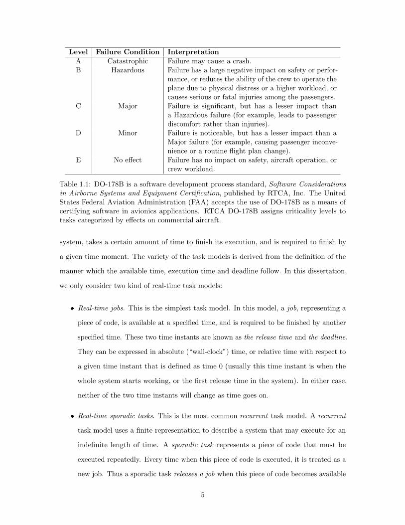
Level Failure Condition Interpretation

A Catastrophic Failure may cause a crash.B Hazardous Failure has a large negative impact on safety or perfor-

mance, or reduces the ability of the crew to operate theplane due to physical distress or a higher workload, orcauses serious or fatal injuries among the passengers.

C Major Failure is significant, but has a lesser impact thana Hazardous failure (for example, leads to passengerdiscomfort rather than injuries).

D Minor Failure is noticeable, but has a lesser impact than aMajor failure (for example, causing passenger inconve-nience or a routine flight plan change).

E No effect Failure has no impact on safety, aircraft operation, orcrew workload.

Table 1.1: DO-178B is a software development process standard, Software Considerationsin Airborne Systems and Equipment Certification, published by RTCA, Inc. The UnitedStates Federal Aviation Administration (FAA) accepts the use of DO-178B as a means ofcertifying software in avionics applications. RTCA DO-178B assigns criticality levels totasks categorized by effects on commercial aircraft.

system, takes a certain amount of time to finish its execution, and is required to finish by

a given time moment. The variety of the task models is derived from the definition of the

manner which the available time, execution time and deadline follow. In this dissertation,

we only consider two kind of real-time task models:

� Real-time jobs. This is the simplest task model. In this model, a job, representing a

piece of code, is available at a specified time, and is required to be finished by another

specified time. These two time instants are known as the release time and the deadline.

They can be expressed in absolute (“wall-clock”) time, or relative time with respect to

a given time instant that is defined as time 0 (usually this time instant is when the

whole system starts working, or the first release time in the system). In either case,

neither of the two time instants will change as time goes on.

� Real-time sporadic tasks. This is the most common recurrent task model. A recurrent

task model uses a finite representation to describe a system that may execute for an

indefinite length of time. A sporadic task represents a piece of code that must be

executed repeatedly. Every time when this piece of code is executed, it is treated as a

new job. Thus a sporadic task releases a job when this piece of code becomes available

5

to be (repeatedly) executed. The task will have a parameter, its relative deadline, so

that when a job is released, it will have its deadline as its release time plus the relative

deadline. The jobs cannot be released infinitely frequently — a minimum inter-arrival

time between any two consecutive job releases is specified, and defined as the task’s

period. In a sporadic task system, it is not possible to know the exact release times of

the jobs in this system. However, in any time interval that is no longer than a task’s

period, there can be at most one job release.

In both task models, it is very important to pre-evaluate the amount of time that a

job requires, in order to assure that no job will miss its deadline. This amount of time is

represented by the job’s worst-case execution time (WCET). In this dissertation, we will not

discuss the techniques that are used to evaluate a job’s execution time. We only assume

that this parameter is known for every job, and a job is guaranteed to be completed if it has

been accumulatively executing for its worst-case execution time.

As a summary, a real-time job is specified by three parameters: its release time, its

deadline, and its worst-case execution time; a real-time sporadic task is also specified by

three parameters: its period, its relative deadline, and its worst-case execution time. A

real-time sporadic task can generate infinitely many real-time jobs.

Now we can define the system using the previously described models. We will consider

the systems that consist of only real-time jobs, or only real-time tasks. To fully describe the

properties of a system, we need more terms, which are provided below.

In this dissertation, only preemptive systems are considered. Preemptive means that at

any time, the scheduling policy can suspend the current executing job, and choose another

job (that can be executed) to execute. Though preemption causes context and state saving

and costs additional time in reality, we assume in this dissertation that any additional

time cost has been bounded by the worst-case execution time. Therefore, in our scheduling

polices, we will not analytically limit the number of preemptions (pragmatic limitations may

be applied, however).

All our previous statements assume hard real-time systems, which means that deadlines

can never be missed, or the scheduling policy will be determined as faulty. Soft real-time

6

systems, which tolerate deadline miss in certain pre-defined manners, will not be discussed

in this dissertation.

The demand of computational resource is an important property of a system. Load

can be used to describe both real-time jobs and real-time recurrent tasks. It denotes the

maximum fraction of processor time demand of a system over any time interval. Utilization

is used only to describe real-time recurrent tasks. It denotes the overall fraction of processor

time demand of a system. Here the time demand over a given interval means the summation

of the WCETs of the jobs that are released in this interval and is required do be finished in

this interval. The formal definitions can be found in Subsection 1.3.3 and 1.3.4.

1.3.2 Overview of Mixed-Criticality Systems

In this subsection, we introduce the detailed mixed-criticality system model by considering

first an example from the domain of unmanned aerial vehicles (UAVs), used for defense

reconnaissance and surveillance. The functionalities on board such UAVs may be classified

into two levels of criticality:

� Level 1: mission-critical functionalities, concerning reconnaissance and surveillance

objectives, like capturing images from the ground, transmitting these images to a base

station, etc.

� Level 2: flight-critical functionalities: to be performed by the aircraft to ensure its

safe operation.

For permission to operate such UAVs over civilian airspace (e.g., for border surveillance), it

is mandatory that its flight-critical functionalities be certified correct by civilian Certification

Authorities (CAs) such as the US Federal Aviation Administration (FAA), which tend to be

very conservative concerning the safety requirements. However, these CAs are not concerned

with the mission-critical functionalities: these must be validated separately by the system

designers (and presumably the customers — those who will purchase the aircraft). The

latter are also interested in ensuring the correctness of the flight-critical functionalities, but

the notion of correctness adopted in validating these functionalities is typically less rigorous

than the one used by the civilian CA’s.

7

This difference in correctness criteria may be expressed by different Worst-Case Execution

Times (WCET) estimates for the execution of a piece of real-time code. In fact, the CA

and the system designers (and other parties responsible for validating the mission-critical

functionalities) will each have their own tools, rules, etc., for estimating WCET; the value

so obtained by the CA is likely to be larger (more pessimistic) than the one obtained by the

system designer. We illustrate via a (contrived) example.

Example 1.1. Consider a system comprised of two jobs: J1 is flight-critical while J2 has

lower mission-critical criticality. Both jobs arrive at time-instant 0, and have their deadlines

at time-instant 10. For i ∈ {1, 2}, let Ci(1) denote the WCET estimate of job Ji as made by

the system designer, and Ci(2) the WCET estimate of job Ji as made by the CA.

As we have stated above, WCET values determined by the CA tend to be larger

than those determined by the system designer. Suppose that C1(1) = 3, C1(2) = 5

and C2(1) = C2(2) = 6. Consider the schedule that first executes J1 and then J2.

� The CA responsible for safety-critical certification would determine that J1 completes

latest by time-instant 5 and meets its deadline. (Note that if the execution time of J1

is 5 then in the worst case it is not possible to complete J2 by its deadline; however,

this CA is not interested in J2; hence the system passes certification.)

� The system designers (and other parties responsible for validating the correctness of

the mission-critical functionalities) determine that J1 completes latest by time-instant

3, and J2 by time-instant 9. Since both jobs complete by their deadlines, the system is

determined to be correct by its designers.

We thus see that the system is deemed as being correct by both the CA and the designers,

despite the fact that the sum of the WCET’s of the jobs at their own criticality levels (6

and 5) exceeds the length of the time window over which they are to execute.

Current practice in safety-critical embedded systems design for certifiability is centered

around the technique of “space-time partitioning”. Loosely speaking, space partitioning

means that each application is granted exclusive access to some of the physical resources

on board the platform, and time partitioning means that the time-line is divided into slots

with each slot being granted exclusively to some (pre-specified) application. Interactions

8

among the partitioned applications may only occur through a severely limited collection of

carefully-designed library routines. This is one of several reservation-based approaches, in

which a certain amount of the capacity of the shared platform is reserved for each application,

that have been considered for designing certifiable mixed-criticality systems. It is known

that reservation-based approaches tend to be pessimistic (in the sense of under-utilizing

platform resource); for instance, a reservation-based approach to the example above would

require that 5 units of execution be reserved for job J1, and 6 units for job J2, over the

interval [0, 10).

1.3.3 Mixed-Criticality Jobs

Although the example that we considered in Section 1.3.2 is characterized by just two

criticality levels, systems may in general have more criticality levels defined. (For instance,

the RTCA DO178-B standard in Table 1.1, widely used in the aviation industry, specifies five

different criticality levels, with the system designer expected to assign one of these criticality

levels to each job. The ISO 26262 standard, used in the automotive domain, specifies four

criticality levels, known in the standard as “safety integrity levels” or SILs.)

Accordingly, the formal model that we use allows for the specification of arbitrarily

many criticality levels. Let L ∈ N+ denote the number of distinct criticality levels in the

mixed-criticality system being modeled.

Definition 1.1. A mixed-criticality job in the mixed-criticality system is characterized by a

4-tuple of parameters: Jj = (aj , dj , χj , Cj), where

� aj ∈ Q+ is the release time;

� dj ∈ Q+ is the deadline, dj ≥ aj ;

� χj ∈ N+ is the criticality of the job;1

� Cj ∈ QL+ is a vector, the k-th coordinate of which specifies the worst-case execution

time (WCET) estimate of job Jj at criticality level k. In a job-specification we will

usually represent it by (Cj(1), . . . , Cj(L)).

1If there are only two criticality levels in the system, we can also use level lo and level hi instead of level1 and 2 when representing χj , and denote this system as a dual-criticality system.

9

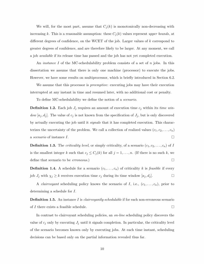
We will, for the most part, assume that Cj(k) is monotonically non-decreasing with

increasing k. This is a reasonable assumption: these Cj(k) values represent upper bounds , at

different degrees of confidence, on the WCET of the job. Larger values of k correspond to

greater degrees of confidence, and are therefore likely to be larger. At any moment, we call

a job available if its release time has passed and the job has not yet completed execution.

An instance I of the MC-schedulability problem consists of a set of n jobs. In this

dissertation we assume that there is only one machine (processor) to execute the jobs.

However, we have some results on multiprocessor, which is briefly introduced in Section 6.2.

We assume that this processor is preemptive: executing jobs may have their execution

interrupted at any instant in time and resumed later, with no additional cost or penalty.

To define MC-schedulability we define the notion of a scenario.

Definition 1.2. Each job Jj requires an amount of execution time cj within its time win-

dow [aj , dj ]. The value of cj is not known from the specification of Jj , but is only discovered

by actually executing the job until it signals that it has completed execution. This charac-

terizes the uncertainty of the problem. We call a collection of realized values (c1, c2, . . . , cn)

a scenario of instance I.

Definition 1.3. The criticality level, or simply criticality, of a scenario (c1, c2, . . . , cn) of I

is the smallest integer k such that cj ≤ Cj(k) for all j = 1, . . . , n. (If there is no such k, we

define that scenario to be erroneous.)

Definition 1.4. A schedule for a scenario (c1, . . . , cn) of criticality k is feasible if every

job Jj with χj ≥ k receives execution time cj during its time window [aj , dj ].

A clairvoyant scheduling policy knows the scenario of I, i.e., (c1, . . . , cn), prior to

determining a schedule for I.

Definition 1.5. An instance I is clairvoyantly-schedulable if for each non-erroneous scenario

of I there exists a feasible schedule.

In contrast to clairvoyant scheduling policies, an on-line scheduling policy discovers the

value of cj only by executing Jj until it signals completion. In particular, the criticality level

of the scenario becomes known only by executing jobs. At each time instant, scheduling

decisions can be based only on the partial information revealed thus far.

10

Definition 1.6. An on-line scheduling policy is correct for instance I if for any non-erroneous

scenario of instance I the policy generates a feasible schedule.

Definition 1.7. An instance I is MC-schedulable if there exists a correct on-line scheduling

policy for instance I.

It is very obvious to see that a MC-schedulable instance I must be also clairvoyant-

schedulable because otherwise there will be scenarios that do not have a feasible schedule.

The MC-schedulability problem is to determine whether a given instance I is MC-

schedulable or not.

Example 1.2. Consider an instance I of a dual-criticality system: a system with L = 2. I

is comprised of 2 jobs: job J1 has criticality level 1 (which is the lower criticality level), and

the other job has the higher criticality level 2.

J1 = (0, 2, 1, (1, 1))

J2 = (0, 3, 2, (1, 3))

For this example instance, any scenario in which c1 and c2, are no larger than 1, has criticality

1; while any scenario not of criticality 1 in which c1 and c2 are no larger than 1, and 3,

respectively, has criticality 2. All remaining scenarios are, by definition, erroneous. It is easy

to verify that this instance is clairvoyantly-schedulable.

Policy S0, described below, is an example of an on-line scheduling policy for instance I:

S0: Execute J2 over [0,1]. If J2 has no remaining execution (i.e., c2 is revealed to be no

greater than 1), then continue with scheduling J1 over (1, 2]; else continue by completely

scheduling J2.

It is easy to see that policy S0 is correct for instance I. However, S0 is not correct if we

modify the deadline of J1 obtaining the following instance I ′:

J1 = (0, 1, 1, (1, 1))

J2 = (0, 3, 2, (1, 3))

After the modification, S0 will cause J1 to miss its deadline if J2 has no remaining

execution at time 1.

11

It is easy to see that I ′ is clairvoyantly schedulable but not MC-schedulable. Any on-line

scheduling policy that starts with executing J1 will cause J2 to miss its deadline if c2 is

revealed to be 3; any on-line scheduling policy that starts with executing J2 will cause J1 to

miss its deadline if c2 is revealed to be no greater than 1.

Speedup factors are a useful conceptual characterization of the effectiveness of a schedul-

ing policy, and may provide valuable insight into the policy’s properties.

Definition 1.8. The speedup factor x for a scheduling policy A is defined as the minimum

factor by which the speed of the processor would need to be increased such that all

instances/systems that are schedulable according to a clairvoyant scheduling policy on a

processor become schedulable under the policy A.

A speedup factor x of the scheduling policy A is called exact if there exists an instance/sys-

tem that is schedulable on processor(s) of speed 1 by an optimal (possibly clairvoyant)

scheduling policy but is not schedulable by A on any processor(s) of speed lower than x.

A scheduling policy A with speedup factor x is called optimal with respect to speedup

factors if there exists an instance/system that is schedulable on processor(s) of speed 1

by the optimal (and clairvoyant) scheduling policy but is not schedulable by any on-line

scheduling policies on any processor(s) of speed lower than x.

Loads are also a useful conceptual characterization of the effectiveness of a scheduling

policy, and provide more in-depth investigation to the relationship among the computational

resource requirement of different criticality levels. Analogous to the load concept in traditional

real-time task models, we find it convenient to define loads of a MC instance I in different

criticality levels:

Definition 1.9. Given a MC instance I, the load of I in criticality level k(1 ≤ k ≤ L) is

defined as the maximum ratio between the sum of criticality level k WCETs in any time

interval and the length of this time interval. It can be written formally as:

`k = max0≤t1<t2

∑Ji : χi≥k∧t1≤ai∧di≤t2

Ci(k)

t2 − t1(1.1)

12

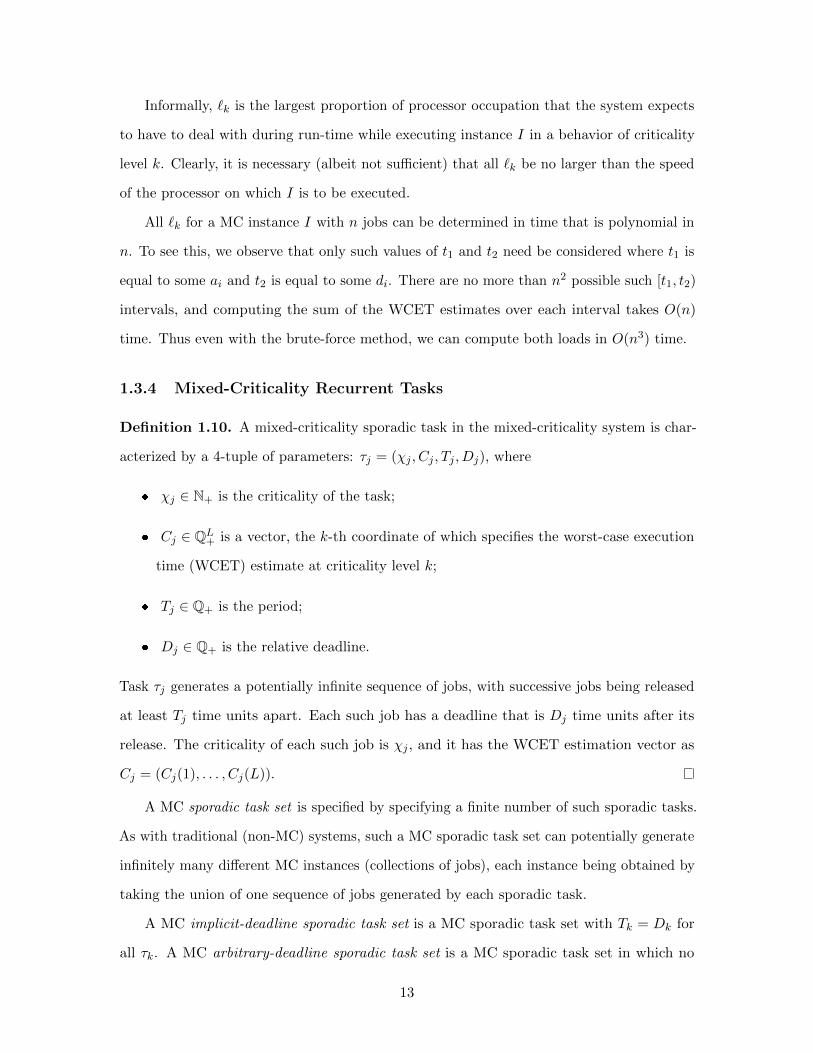
Informally, `k is the largest proportion of processor occupation that the system expects

to have to deal with during run-time while executing instance I in a behavior of criticality

level k. Clearly, it is necessary (albeit not sufficient) that all `k be no larger than the speed

of the processor on which I is to be executed.

All `k for a MC instance I with n jobs can be determined in time that is polynomial in

n. To see this, we observe that only such values of t1 and t2 need be considered where t1 is

equal to some ai and t2 is equal to some di. There are no more than n2 possible such [t1, t2)

intervals, and computing the sum of the WCET estimates over each interval takes O(n)

time. Thus even with the brute-force method, we can compute both loads in O(n3) time.

1.3.4 Mixed-Criticality Recurrent Tasks

Definition 1.10. A mixed-criticality sporadic task in the mixed-criticality system is char-

acterized by a 4-tuple of parameters: τj = (χj , Cj , Tj , Dj), where

� χj ∈ N+ is the criticality of the task;

� Cj ∈ QL+ is a vector, the k-th coordinate of which specifies the worst-case execution

time (WCET) estimate at criticality level k;

� Tj ∈ Q+ is the period;

� Dj ∈ Q+ is the relative deadline.

Task τj generates a potentially infinite sequence of jobs, with successive jobs being released

at least Tj time units apart. Each such job has a deadline that is Dj time units after its

release. The criticality of each such job is χj , and it has the WCET estimation vector as

Cj = (Cj(1), . . . , Cj(L)).

A MC sporadic task set is specified by specifying a finite number of such sporadic tasks.

As with traditional (non-MC) systems, such a MC sporadic task set can potentially generate

infinitely many different MC instances (collections of jobs), each instance being obtained by

taking the union of one sequence of jobs generated by each sporadic task.

A MC implicit-deadline sporadic task set is a MC sporadic task set with Tk = Dk for

all τk. A MC arbitrary-deadline sporadic task set is a MC sporadic task set in which no

13

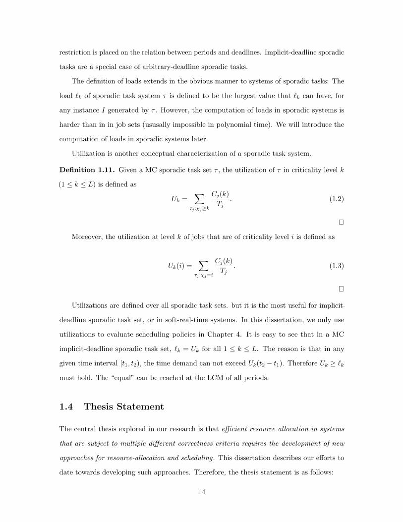
restriction is placed on the relation between periods and deadlines. Implicit-deadline sporadic

tasks are a special case of arbitrary-deadline sporadic tasks.

The definition of loads extends in the obvious manner to systems of sporadic tasks: The

load `k of sporadic task system τ is defined to be the largest value that `k can have, for

any instance I generated by τ . However, the computation of loads in sporadic systems is

harder than in in job sets (ususally impossible in polynomial time). We will introduce the

computation of loads in sporadic systems later.

Utilization is another conceptual characterization of a sporadic task system.

Definition 1.11. Given a MC sporadic task set τ , the utilization of τ in criticality level k

(1 ≤ k ≤ L) is defined as

Uk =∑

τj :χj≥k

Cj(k)

Tj. (1.2)

Moreover, the utilization at level k of jobs that are of criticality level i is defined as

Uk(i) =∑

τj :χj=i

Cj(k)

Tj. (1.3)

Utilizations are defined over all sporadic task sets. but it is the most useful for implicit-

deadline sporadic task set, or in soft-real-time systems. In this dissertation, we only use

utilizations to evaluate scheduling policies in Chapter 4. It is easy to see that in a MC

implicit-deadline sporadic task set, `k = Uk for all 1 ≤ k ≤ L. The reason is that in any

given time interval [t1, t2), the time demand can not exceed Uk(t2 − t1). Therefore Uk ≥ `k

must hold. The “equal” can be reached at the LCM of all periods.

1.4 Thesis Statement

The central thesis explored in our research is that efficient resource allocation in systems

that are subject to multiple different correctness criteria requires the development of new

approaches for resource-allocation and scheduling . This dissertation describes our efforts to

date towards developing such approaches. Therefore, the thesis statement is as follows:

14

New methods can be discovered to schedule real-time systems with multiple

criticalities. The methods can supply multiple temporal predictability assertions

with respect to multiple WCET specifications. The assertions can be defined

and measured through a formalized description. The methods can be efficiently

implemented with acceptable computational complexities.

1.5 Contributions

The first and basic question after proposing the model is a purely algorithmic problem:

how to schedule mixed-criticality jobs, with specified release-times and deadlines, when

no dependencies among these jobs exist? The new assumptions in the mixed-criticality

model require new principles. While the traditional real-time system scheduling favors

only urgent jobs, mixed-criticality systems must also prioritize high-criticality jobs so that

they are prepared for potentially long execution. The compromise between urgency and

significance results in exponential choices, and hence leads to the fact that mixed-criticality

scheduling is NP-hard in the strong sense (Baruah et al., 2010c, 2012b). In the absence

of an efficient optimal algorithm, the first efficient approximation algorithm named Own-

Criticality-Based-Priority (OCBP) algorithm is proposed to generate a correct priority

list for mixed-criticality jobs in polynomial time. This algorithm recursively searches a

lowest-priority job by simulating the behavior of all other jobs according to the candidate’s

own criticality. The performance of this algorithm is quantified in the form of speedup

factors. The speedup factor of OCBP algorithm is 1.618 (the golden ratio) for two criticality

levels, which is a significant improvement compared with current practice’s speedup factor 2,

and is proved to be the minimal speedup factor the on-line scheduling policies can reach.

The speedup factors for more criticality levels are also calculated, and it is shown that the

OCBP algorithm gives an O(L/ lnL) speedup factor to L criticality levels as opposed to

the O(L) speedup factor of the current worst-case reservation method. A more in-depth

investigation to the relationship among the processor loads of different criticality levels is

also made so that we understand the connections among the criticality levels more precisely

and quantitatively.

15

The more general and popular abstraction to real-time tasks in real-time system research

is the sporadic task model, where the jobs are released recurrently with minimum time gaps.

Thus the second question to the mixed-criticality system is whether the mixed-criticality

sporadic tasks can be efficiently scheduled. In order to answer this question, the classic

Earliest-Deadline-First (EDF) algorithm is specialized to support mixed-criticality systems.

In the traditional real-time scheduling, EDF is proved to be an optimal exact algorithm

on preemptive uniprocessor platform. Its philosophy of favoring urgent jobs, in the form

of always choosing the job with the earliest deadline to execute, provably maximizes the

use of processor capacity in the traditional real-time systems. Yet in order to promote

high-criticality tasks in mixed-criticality systems as mentioned above, these tasks will be

given earlier virtual deadlines to reflect their importance over low-criticality tasks. This

modified EDF algorithm (named EDF-VD, where VD stands for virtual deadlines) has

a speedup factor of 4/3 for mixed-criticality sporadic systems with two criticality levels

and implicit deadlines, while this factor is also shown as minimal for the mixed-criticality

implicit-deadline sporadic task systems. This modified EDF algorithm is also extended

to mixed-criticality arbitrary-deadline sporadic task sets, and is proved to have a speedup

factor as 1.83.

Besides these two main contributions, other research results will also be mentioned in

Chapter 6. The OCBP algorithm is generalized according to the sporadic task model. The

challenge is that a sporadic task can release infinite jobs at indefinite time instants. An

on-line priority adjustment technique is proposed to deal with unanticipated job releases

while preserving the speedup factor. It uses a priority list computed by the OCBP algorithm

for a longest and densest possible job release sequence, and recomputes the priority list to

dynamically secure the correctness of the ongoing schedule at the instant when a new job

releases. The EDF-VD algorithm is extended to the main two categories in the multiprocessor

scheduling theory: the global multiprocessor scheduling (tasks and jobs can migrate among

processors) and the partitioned multiprocessor scheduling (tasks are assigned to dedicated

processors). An initial effort is made on analyzing the mixed-criticality multiprocessors

scheduling problem. Both based-on the EDF-VD algorithm, the global scheduling policy

adjusts the deadlines of high-criticality tasks so that the system is schedulable when the

16

tasks are globally scheduled according to the adjusted deadlines; whereas the partitioned

scheduling policy partitions the tasks to subsets so that each subset is schedulable by

EDF-VD on a uniprocessor. The speedup factors for these algorithms are respectively 3.24

and 2.67, as opposed to the speedup factor 4 of the naive worst-case reservation method.

17

CHAPTER 2

Prior Work

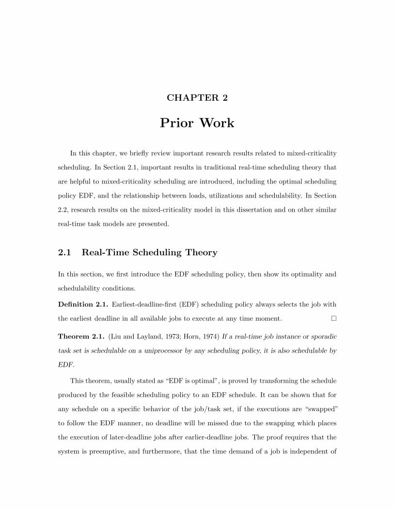
In this chapter, we briefly review important research results related to mixed-criticality

scheduling. In Section 2.1, important results in traditional real-time scheduling theory that

are helpful to mixed-criticality scheduling are introduced, including the optimal scheduling

policy EDF, and the relationship between loads, utilizations and schedulability. In Section

2.2, research results on the mixed-criticality model in this dissertation and on other similar

real-time task models are presented.

2.1 Real-Time Scheduling Theory

In this section, we first introduce the EDF scheduling policy, then show its optimality and

schedulability conditions.

Definition 2.1. Earliest-deadline-first (EDF) scheduling policy always selects the job with

the earliest deadline in all available jobs to execute at any time moment.

Theorem 2.1. (Liu and Layland, 1973; Horn, 1974) If a real-time job instance or sporadic

task set is schedulable on a uniprocessor by any scheduling policy, it is also schedulable by

EDF.

This theorem, usually stated as “EDF is optimal”, is proved by transforming the schedule

produced by the feasible scheduling policy to an EDF schedule. It can be shown that for

any schedule on a specific behavior of the job/task set, if the executions are “swapped”

to follow the EDF manner, no deadline will be missed due to the swapping which places

the execution of later-deadline jobs after earlier-deadline jobs. The proof requires that the

system is preemptive, and furthermore, that the time demand of a job is independent of

the moment and order of its execution. Therefore, this scheduling policy is not optimal any

more when applied to mixed-criticality task models, because if the execution order of the

jobs is changed, the time demand may differ — low-criticality jobs may be ignored after the

high-criticality behavior is revealed.

Example 2.1. Consider an dual-criticality job instance I that consists of two jobs J1 and

J2. As we denote a job as Jj = (aj , dj , χj , Cj), the two jobs are represented as

J1 = (0, 4, 2, (2, 4))

J2 = (1, 3, 1, (1, 1)).

Now if we consider the EDF scheduling policy in low-criticality behavior of this instance,

the run-time behavior will be: (1) at time instant 0, start executing J1; (2) at time instant

1, suspend J1 and start executing J2, because J2 is available to execute and has the earliest

deadline in all available jobs (J1 and J2); (3) at time instant 2, J2 is completed so start

executing J2 again; (4) at time instant 3, complete J1 (because it is the low-criticality

behavior) which meets its deadline.

It is important to note that even if we do not know the parameters (including release

times, deadlines and WCETs) of all or any jobs, the scheduling decisions made by EDF

scheduling policy will remain the same. Like in the example, assuming that J2’s release

time isn’t known beforehand, at time instant 1 when J2 is actually released, EDF scheduling

policy will pick J2 for execution.

However, if we consider the high-criticality behavior of this instance which includes

a criticality change, EDF scheduling policy isn’t correct (thus non-optimal) any more. If

we simulate the run-time behavior again, it will be: (1) at time instant 0, start executing

J1; (2) at time instant 1, suspend J1 and start executing J2; (3) at time instant 2, J2 is

completed so start executing J2 again; (4) at time instant 5, complete J1 (because it is the

high-criticality behavior) which misses its deadline.

A correct scheduling policy for this example can be a priority-based policy: assign J1

a higher priority than J2. Therefore, J1 will keep executing until time instant 2. If it is

completed by then, J2 will be executed and meet its deadline; otherwise keep executing J1

19

and discard J2, because J2 can miss its deadline validly if J1 uses more than C1(1) = 2 time

units.

Theorem 2.2. (Baruah et al., 1990) A real-time job instance or sporadic task set is

schedulable by EDF if and only if its load is no greater than 1.

The original theorem in (Baruah et al., 1990) is presented in the form of DBF (demand

bound function). Basically, it states the fact that as long as the time demand does not

exceed the processor capacity in any time interval (or briefly “processor is not over-utilized”),

the system is schedulable by EDF.

Though it appears that the calculation of the load of a system is a good method to

perform a schedulability test, the following two theorems show that the calculation for

sporadic task sets is computationally expensive.

Theorem 2.3. (Baruah et al., 1990; Eisenbrand and Rothvoß, 2010) The problem of deciding

whether a real-time arbitrary-deadline sporadic task set is schedulable is coNP-hard.

Theorem 2.4. (Baruah et al., 1990) The load of a real-time arbitrary-deadline sporadic

task set can be computed in pseudo-polynomial time if the utilization of the task set is less

than 1.

Theorem 2.3 and 2.4 indicate that there is no polynomial-time schedulability test for

arbitrary-deadline sporadic task sets, even though it is known that EDF is the optimal

scheduling policy. However, for implicit-deadline sporadic task sets, the schedulability test

is much more efficient.

Theorem 2.5. (Liu and Layland, 1973) A real-time implicit-deadline sporadic task set is

schedulable by EDF if and only if its utilization is no greater than 1.

Theorem 2.5 is discovered much earlier than Theorem 2.2. Actually, Theorem 2.5 is a

corollary of Theorem 2.2 because the utilization is equal to the load for an implicit-deadline

sporadic task set. Because Theorem 2.5 provides a very efficient schedulability test, it is

very widely applied and cited.

The theorems in this section provide the basic expectations to time complexities of

schedulability tests for different real-time task models. In Chapter 3, the load-based

20

schedulability test shows the relationship between schedulability and loads in mixed-criticality

jobs, but it is also an efficient schedulability test since the calculation of loads for real-time

jobs can be done in polynomial time. In Chapter 4, the utilization-based schedulability

test is applied to mixed-criticality implicit-deadline sporadic tasks. In Chapter 5, the

load-based schedulability test is applied to mixed-criticality arbitrary-deadline sporadic

tasks. In contrast to the results in classic real-time task models, none of these tests in this

dissertation keep optimal. The reason why only approximate schedulability tests are pursued

is introduced in the following section.

2.2 Mixed-Criticality Scheduling Theory

In this section, we discuss the development of the mixed-criticality task model and scheduling

theory, important results in mixed-criticality scheduling theory, and several real-time task

models that are similar to the mixed-criticality task model.

The mixed-criticality scheduling problem arises from multiple certification requirements.

Vestal presents the concept of applying more conservative worst-case execution time param-

eters to safety-critical tasks in preemptive uniprocessor recurrent real-time task systems, in

order to obtain higher confidence of timing assurance at higher certification level (Vestal,

2007). Also in that paper, the multi-criticality task model is formalized and the fixed-priority

response time analysis is conducted. Later in (Baruah and Vestal, 2008), Baruah and Vestal

propose a more precise schedulability test in accordance with a hybrid scheduling algorithm

that conflates fixed-task-priority scheduling and EDF based on the multi-criticality task

model in (Vestal, 2007). The mixed-criticality scheduling model in this dissertation which

formalized the behavior of tasks and correctness of algorithms is presented by Baruah et

al. in a more abstracted manner in (Baruah et al., 2010b). The most significant change is

that the multi-criticality task model in (Vestal, 2007) and (Baruah and Vestal, 2008) requires

that the low-criticality tasks are assigned a larger WCET, and must execute for its WCET

in high-criticality behavior; however, in mixed-criticality scheduling model, the run-time

scheduling algorithm is permitted to prevent low-criticality tasks from being executed if the

algorithm detects high-criticality behavior.

21

In (Baruah et al., 2010c, 2012b), the MC-schedulability problem in mixed-criticality

task model is proven to be NP-hard in the strong sense even in very simple cases.

Theorem 2.6. (Baruah et al., 2010c, 2012b) MC-schedulability problem is NP-hard in the

strong sense, even when all release times are identical and there are only two criticality

levels.

The strong NP-hardness of MC-schedulability problem indicates that neither polynomial

nor pseudo-polynomial time algorithms exist to exactly decide whether there is a scheduling

policy for a mixed-criticality job instance or task set. As a result, research on scheduling

mixed-criticality systems only focuses on seeking efficient approximation algorithms. The

OCBP (Own-Criticality-Based-Priority) algorithm for mixed-criticality jobs is proposed and

analyzed in (Baruah et al., 2010b), (Baruah et al., 2010a), (Baruah et al., 2010c) and (Baruah

et al., 2012b). This algorithm will be described in detail in Chapter 3. Park and Kim propose

a new algorithm using dynamic programming to schedule dual-criticality jobs in (Park and

Kim, 2011), which dominates OCBP algorithm for two criticality levels. Baruah and Fohler

propose a time-triggered algorithm to schedule dual-criticality jobs, with the 1.618 speedup

factor as well (Baruah and Fohler, 2011). This algorithm is the first non-work-conserving

mixed-criticality scheduling algorithm (non-work-conserving means that the processor can

be idle when there is at least one job available). The connection between the computational

resource demands in each criticality level for dual-criticality mixed-criticality jobs scheduled

by OCBP algorithm is further investigated in (Li and Baruah, 2010b). This result will be

extended to an arbitrary number of criticality levels in Chapter 3.

A more widely-used real-time task model is the sporadic task model where the jobs

are released recurrently with minimal gaps between adjacent releases, instead of having

independently specified release times in the independent job model. The mixed-criticality

model is hence extended to mixed-criticality sporadic task systems. The OCBP algorithm is

enhanced to support sporadic systems in (Li and Baruah, 2010a) by applying the algorithm

on a sufficiently long job release sequence to get an initial priority list, and updating the

priority list on-line at certain time instants to maintain the correctness of the priority list.

Both the off-line schedulability test and run-time updating will cost pseudopolynomial time.

22

In (Guan et al., 2011), Guan et al. improve this algorithm to a new version named PLRS

(Priority-List-Reuse-Scheduling) algorithm, which updates the priority list in O(n2) time.

The EDF (Earliest-Deadline-First) algorithm is the optimal scheduling policy for classic

uniprocessor real-time sporadic task systems, thus it has been modified to support mixed-

criticality sporadic task systems in various ways. Baruah et al. propose EDF-VD (EDF with

Virtual Deadlines) algorithm that schedules mixed-criticality implicit-deadline sporadic task

systems (Baruah et al., 2011a). EDF-VD algorithm shrinks the high-criticality deadlines

proportionally by a certain factor so that the high-criticality tasks will be promoted by

the EDF scheduler. In (Baruah et al., 2011a), an O(n) time sufficient schedulability test

with derived speedup factors is proposed while the logarithmic run-time complexity of

EDF scheduler is preserved. The speedup factor of EDF-VD algorithm for dual-criticality

system is shown as 1.618 in (Baruah et al., 2011a). The speedup factor is improved to

1.33 in (Baruah et al., 2012a). It is also shown that EDF-VD algorithm is optimal with

respect to speedup factors in all scheduling policies for dual-criticality implicit-deadline

systems in (Baruah et al., 2012a). The analysis and proof of optimal speedup factor will be

shown in Chapter 4. Ekberg and Yi propose a new EDF-based algorithm for dual-criticality

constrained-deadline systems that formulates the demand-bound function in each criticality,

assigns every high-criticality task an adjusted relative deadline and schedules the system by

EDF according to the adjusted deadlines in (Ekberg and Yi, 2012). The adjusted deadlines

are calculated through an off-line procedure which tunes the deadlines in pseudopolynomial

time so that the time demand never exceeds the time supply in each criticality.

There is a special class of scheduling policies, fixed-priority scheduling where all jobs

in one task share the same priority. In (Dorin et al., 2010), Dorin et al. showed that

the fixed-priority scheduling of mixed-criticality sporadic task systems with L criticality

levels cannot have a speedup factor smaller than L. In (Baruah et al., 2011b), Baruah et

al. proposed a fixed-priority scheduling algorithm named AMC (Adaptive Mixed-Criticality)

algorithm, which effectively undertakes the response-time analysis and assign priorities to

tasks in mixed-criticality constrained-deadline sporadic task systems. Santy et al. discuss

the possibility of allowing low-criticality tasks to proceed with their execution even if

high-criticality behavior is detected under fixed-priority scheduling in (Santy et al., 2012).

23

The multiprocessor mixed-criticality scheduling problem has seldom been studied before

(Li and Baruah, 2012). In (Mollison et al., 2010), Mollison et al. establish a hierarchical

scheduling framework that aims at practically scheduling tasks in multiple criticality levels

on a multi-core platform. Herman et al. present the overhead, isolation and synchronization

issues when implementing this framework robustly in real-time operating systems in (Herman

et al., 2012). However, in (Mollison et al., 2010) and (Herman et al., 2012), the periods of

tasks are assumed harmonic and monotonic with respect to criticality levels. In (Baruah

et al., 2011a), Baruah et al. show a modified multiprocessor version of OCBP algorithm

that schedules dual-criticality independent jobs on identical multiprocessors, and prove the

existence of a polynomial-time approximation scheme (PTAS) that partitions dual-criticality

sporadic tasks to multiprocessors with EDF-VD scheduler. In (Pathan, 2012), Pathan

studies the fixed-priority global and partitioned scheduling on multiprocessors and provides

a schedulability test based-on response-time analysis.

Some criticality-related but not certification-cognizant problems are discussed in other

papers. De Niz et al. propose another mixed-criticality system model in (de Niz et al., 2009)

and (Lakshmanan et al., 2010) where at most one high-criticality task can overrun. Their

solution, zero-slack scheduling seeks the critical instant after which the high-criticality tasks

will have insufficient time to meet their deadlines when overloaded. In (Pellizzoni et al.,

2009) and (Yun et al., 2012), Pellizzoni et al. focuses on the the technique of temporal and

physical isolation among different criticality levels.

Many other papers discuss problems that are similar to the mixed-criticality scheduling

problem. The mode-change protocol research, like in (Real and Crespo, 2004), (Phan

et al., 2009) and (Phan et al., 2011), focuses on the response-time analysis and resource

allocation techniques when the task set is changed and the pending/partially-processed jobs

are required to be completed, transferred or discarded. It deals with a much more general

scenario than criticality change in mixed-criticality system, yet does not typically provide

specific mixed-criticality scheduling policies. The overloaded real-time scheduling research,

like in (Baruah and Haritsa, 1997) and (Koren and Shasha, 2003), tries to maximize the ratio

of the completed tasks over all tasks, if possible overloading happens. However, this model

is not able to address our problem that different sets of deadlines should be assertively met

24

on different criticality levels. The bandwidth-preserving servers and compositional analysis

research, like in (Ghazalie and Baker, 1995) and (Shin and Lee, 2004), focuses on how to

ensure that a task set will not use more than a specified processor capacity budget. Though

we have similar requirements in mixed-criticality systems (low-criticality tasks must not

overrun), the tools in bandwidth-preserving servers and compositional analysis are aimed

at providing much more than our requirement. In mixed-criticality systems, we need to

guarantee that no single job will overrun, which can be implemented by simply monitoring

a single job’s execution time; however, bandwidth-preserving servers and compositional

analysis are used to enforce that a collection of jobs/tasks must not use more than a given

proportion of the processor capacity, which is too complicated and beyond the necessary

functionalities we need.

25

CHAPTER 3

Scheduling Mixed-Criticality Jobs

In this chapter, we discuss the scheduling of mixed-criticality jobs. In Section 3.2, we

briefly introduce a straightforward worst-case reserving solution that simply maps mixed-

criticality jobs to a traditional real-time jobs. Then in Section 3.3, 3.4 and 3.5, we introduce

our solution, OCBP algorithm, including its detailed description, a load-based schedulability

test, and the evaluation of its performance through the speedup factor metric.

3.1 Overview

Since MC-schedulability is intractable even for dual-criticality instances, we concentrate

here on sufficient (rather than exact) MC-schedulability conditions that can be verified in

polynomial time. We study two widely-used scheduling policies that yield such sufficient

conditions and compare their capabilities under the resource augmentation metric: the

minimum speed of the processor needed for the algorithm to schedule all instances that

are MC-schedulable on a unit-speed processor. We show that the second policy we present

outperforms the first one in terms of the resource augmentation metric, in the sense that it

needs lower-speed processors to ensure such schedulability.

Run-time support for mixed criticality. In scheduling mixed-criticality systems, the

kinds of performance guarantees that can be made depend upon the forms of support that

are provided by the run-time environment upon which the system is being implemented. A

particularly important form of platform support is the ability to monitor the execution of

individual jobs, i.e., being able to determine how long a particular job has been executing.

Why is such a facility useful? In essence, knowledge regarding how long individual

jobs have been executing allows the system to become aware, during run-time, when the

criticality level of the scenario changes from a value k to the next-higher value k + 1, due to

some job executing beyond its level-k WCET without signalling completion; this information

can then be used by the run-time scheduling and dispatching algorithm to no longer execute

criticality-k jobs once the transition has occurred.

In the remainder of this section, we assume that this facility to monitor the execution

of individual jobs is provided by the run-time environment. We may therefore make the

assumption that for each job Jj , Cj(k) = Cj(χj) for all k ≥ χj . That is, no job executes

longer than the WCET at its own specified criticality. This is without loss of generality for

any correct scheduling policy: any such policy will immediately interrupt (and no longer

schedule) a job Jj if its execution time cj exceeds Cj(χj), since this makes the scenario of

higher criticality level than χj , and therefore the completion of Jj becomes irrelevant for

the scenario.

3.2 Worst-Case Reservation Scheduling

One straightforward approach is to map each MC job Jj into a traditional (i.e., non-MC) job

with the same arrival time aj and deadline dj and processing time cj = Cj(χj) = maxk Cj(k)

(by monotonicity), and determine whether the resulting collection of traditional jobs is

schedulable using some preemptive single machine scheduling algorithm such as the Earliest

Deadline First (EDF) rule1. This test can clearly be done in polynomial time. We will refer

to mixed-criticality instances that are MC-schedulable by this test as worst-case reservation

schedulable (WCR-schedulable) instances.

Theorem 3.1. If an instance is WCR-schedulable on a processor, then it is MC-schedulable

on the same processor. Conversely, if an instance I with L criticality levels is MC-schedulable

on a given processor, then I is WCR-schedulable on a processor that is L times as fast, and

this factor is tight.

1In fact, this approach forms the basis of current practice, as formulated in the ARINC-653 standard:each Jj is guaranteed Cj(χj) units of execution in a time partitioned schedule, obtained by partitioning thetime-line into distinct slots and only permitting particular jobs to execute in each such slot.

27

Proof. If instance I is WCR-schedulable then for each job the maximum amount of time

the job may execute is reserved between its arrival time and its deadline. Hence it is

MC-schedulable.

Suppose now that instance I is MC-schedulable. If we were to use a separate processor

for each of the L criticality levels, then each job will receive its maximum processing time

between arrival time and deadline e.g. by using EDF on the machine corresponding to its

criticality level. Hence, by processer sharing, WCR-schedulability on one processor of speed

L times faster follows immediately.

Finally, we show that there exist instances with L criticality levels that are MC-

schedulable on a given processor, but not WCR-schedulable on a processor that is less

than L times as fast.

Consider the instance I comprised of the following L jobs:

J1 = (0, 1, 1, (1, 1, . . . , 1, 1))

J2 = (0, 1, 2, (0, 1, . . . , 1, 1))

......

JL = (0, 1, L, (0, 0, . . . , 0, 1))

This instance is MC-schedulable on a unit-speed processor by the scheduling policy of

assigning priority in criticality-monotonic (CM) order: JL, JL−1, . . . .J2, J1. Any scenario

(c1, c2, . . . , cL) with ch > 0, h ≥ 2, and cj = 0 for all j > h, has criticality level h, hence

all jobs of lower criticality level, in particular J1, are not obliged to meet their deadline,

and job h will meet its deadline. On the other hand, in any scenario of criticality level 1,

c2 = c3 = . . . = cL = 0 and c1 ∈ [0, 1], hence all jobs meet their deadline.

However, WCR-schedulability requires that each job Jj is executed for Cj(χj) = 1,

j = 1, . . . , L before common deadline 1, which clearly can only be achieved on a processor

with speed at least L.

28

3.3 Own-Criticality-Based-Priority Algorithm

We now consider another schedulability condition, OCBP-schedulability, that offers a

performance guarantee (as measured by the processor speedup factor) that is superior to the

performance guarantee offered by the WCR-approach. OCBP-schedulability is a constructive

test: we determine off-line, before knowing the actual execution times, a total ordering of

the jobs in a priority list and for each scenario execute at each moment in time the available

job with the highest priority.

The priority list is constructed recursively using the approach commonly referred to

in the real-time scheduling literature as the “Audsley approach” (Audsley, 1991, 1993); it

is also related to a technique introduced by Lawler (Lawler, 1973). First determine the

lowest priority job: Job Ji may be assigned the lowest priority if there is at least Ci(χi)

time between its release time and its deadline available when every other job Jj is executed

before Ji for Cj(χi) time units (the WCET of job Jj according to the criticality level of job i).

This can be determined by simulating the behavior of the schedule under the assumption

that every job other than Ji has priority over Ji (and ignoring whether these other jobs meet

their deadlines or not — i.e., they may execute under any relative priority ordering, and will

continue executing even beyond their deadlines). The procedure is repeatedly applied to the

set of jobs excluding the lowest priority job, until all jobs are ordered, or at some iteration a

lowest priority job does not exist. If job Ji has higher priority than job Jj we write Ji B Jj .

Because the priority of a job is based only on its own criticality level, the instance I is

called Own Criticality Based Priority OCBP)-schedulable if we find a complete ordering of

the jobs.

If at some recursion in the algorithm no lowest priority job exists, we say the instance is

not OCBP-schedulable. We can simply argue that this does not mean that the instance is

not MC-schedulable: Suppose that scheduling according to the fixed priority list J1, J2, J3

with χ2 = 1 and χ1 = χ3 = 2, proves the instance to be schedulable. It may not be

OCBP-schedulable since this does not take into account that J2 does not need to be executed

at all if J1 receives execution time c1 > C1(1).

29

It is evident that the OCBP priority list for an instance of n jobs can be determined in

time polynomial in n: at most n jobs need be tested to determine whether they can be the

lowest-priority job; at most (n− 1) jobs whether they can be the 2nd-lowest priority jobs;

etc. Therefore, at most n+ (n− 1) + · · ·+ 3 + 2 + 1 = O(n2) simulations need be run, and

each simulation takes polynomial time.

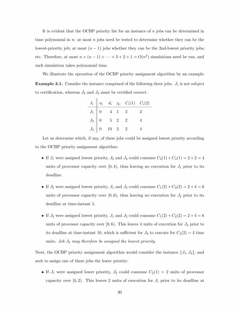
We illustrate the operation of the OCBP priority assignment algorithm by an example:

Example 3.1. Consider the instance comprised of the following three jobs. J1 is not subject

to certification, whereas J2 and J3 must be certified correct.

Ji ai di χi Ci(1) Ci(2)

J1 0 4 1 2 2

J2 0 5 2 2 4

J3 0 10 2 2 4

Let us determine which, if any, of these jobs could be assigned lowest priority according

to the OCBP priority assignment algorithm:

� If J1 were assigned lowest priority, J2 and J3 could consume C2(1) +C3(1) = 2 + 2 = 4

units of processor capacity over [0, 4), thus leaving no execution for J1 prior to its

deadline.

� If J2 were assigned lowest priority, J1 and J3 could consume C1(2) +C3(2) = 2 + 4 = 6

units of processor capacity over [0, 6), thus leaving no execution for J2 prior to its

deadline at time-instant 5.

� If J3 were assigned lowest priority, J1 and J2 could consume C1(2) +C2(2) = 2 + 4 = 6

units of processor capacity over [0, 6). This leaves 4 units of execution for J3 prior to

its deadline at time-instant 10, which is sufficient for J3 to execute for C3(2) = 4 time

units. Job J3 may therefore be assigned the lowest priority.

Next, the OCBP priority assignment algorithm would consider the instance {J1, J2}, and

seek to assign one of these jobs the lower priority:

� If J1 were assigned lower priority, J2 could consume C2(1) = 2 units of processor

capacity over [0, 2). This leaves 2 units of execution for J1 prior to its deadline at

30

time-instant 4, which is sufficient for J1 to execute for C1(1) = 2 time units. Job J1

may therefore be assigned the lowest priority from among {J1, J2}.

� It may be verified that J2 cannot be assigned the lowest priority from among {J1, J2}.

If we were to do so, then J1 could consume C1(2) = 2 units of processor capacity

over [0, 2). This leaves 3 units of execution for J1 prior to its deadline at time-instant

5, which is not sufficient for J2 to execute for the C2(2) = 4 time units it needs to

complete on time.2

The final OCBP priority ordering is therefore as follows. Job J2 has the greatest priority,

job J1 has the next-highest priority, and J3 has the lowest priority. It may be verified that

scheduling according to these priorities is a correct MC scheduling strategy for the instance

{J1, J2, J3}.

3.4 Load-Based OCBP Schedulability Test

The following lemma shows that OCBP-schedulability implies MC-schedulability.

Lemma 3.1. If an instance is OCBP-schedulable on a processor, then it is MC-schedulable

on the same processor.

Proof. Suppose that I is OCBP-schedulable and suppose, after renumbering jobs, that

J1 B J2 B · · ·B Jn. Notice that in every scenario of criticality level χk, the criticality level of

job Jk, each job Jj has cj ≤ Cj(χk). OCBP-schedulability of I implies that Jk can receive

Ck(χk) units of execution before its deadline if each Ji ∈ {J1, . . . , Jk−1} executes for no

more than Ci(χk) units.

The following theorem provides quantitative load bounds on OCBP scheduling algorithms,

and also leads to the speedup factor result of OCBP scheduling algorithm.

2We point out that OCBP will not actually perform this step of verifying that J2 cannot be assignedlowest priority since it has already determined, above, that J1 may be assigned lowest priority.

31

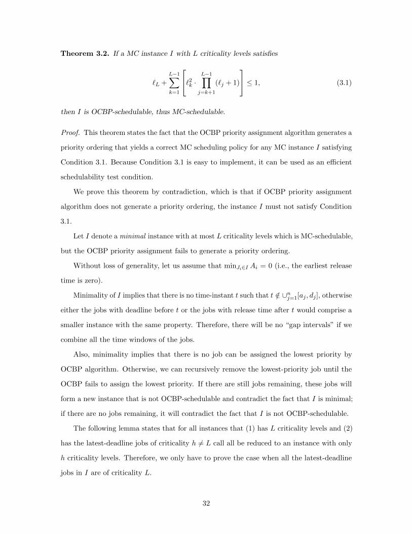
Theorem 3.2. If a MC instance I with L criticality levels satisfies

`L +

L−1∑k=1

`2k · L−1∏j=k+1

(`j + 1)

≤ 1, (3.1)

then I is OCBP-schedulable, thus MC-schedulable.

Proof. This theorem states the fact that the OCBP priority assignment algorithm generates a

priority ordering that yields a correct MC scheduling policy for any MC instance I satisfying

Condition 3.1. Because Condition 3.1 is easy to implement, it can be used as an efficient

schedulability test condition.

We prove this theorem by contradiction, which is that if OCBP priority assignment

algorithm does not generate a priority ordering, the instance I must not satisfy Condition

3.1.

Let I denote a minimal instance with at most L criticality levels which is MC-schedulable,

but the OCBP priority assignment fails to generate a priority ordering.

Without loss of generality, let us assume that minJi∈I Ai = 0 (i.e., the earliest release

time is zero).

Minimality of I implies that there is no time-instant t such that t /∈ ∪nj=1[aj , dj ], otherwise

either the jobs with deadline before t or the jobs with release time after t would comprise a

smaller instance with the same property. Therefore, there will be no “gap intervals” if we

combine all the time windows of the jobs.

Also, minimality implies that there is no job can be assigned the lowest priority by

OCBP algorithm. Otherwise, we can recursively remove the lowest-priority job until the

OCBP fails to assign the lowest priority. If there are still jobs remaining, these jobs will

form a new instance that is not OCBP-schedulable and contradict the fact that I is minimal;

if there are no jobs remaining, it will contradict the fact that I is not OCBP-schedulable.

The following lemma states that for all instances that (1) has L criticality levels and (2)

has the latest-deadline jobs of criticality h 6= L call all be reduced to an instance with only

h criticality levels. Therefore, we only have to prove the case when all the latest-deadline

jobs in I are of criticality L.

32

Lemma 3.2. Any job in I with the latest deadline must be of criticality L.

Proof. First, we assume that Theorem 3.2 holds for all instances with criticality level no

higher than L. Because when L = 1, the Condition 3.1 becomes `1 ≤ 1, which is trivially

true, we can build the proof by induction based on this assumption.

Now suppose that a job Ji with χi = h < L has the latest deadline. Create from I an

instance Ih with h levels by “truncating” all jobs with criticality level greater than h to

their worst-case level-h scenarios:

Jj = (aj , dj , χj , (Cj(1), . . . , Cj(L))) ∈ I →

J ′j = (aj , dj ,min(χj , h), (Cj(1), . . . , Cj(h))) ∈ Ih.

Clearly, because the WCETs and criticality levels of all jobs in Ih are no greater than

those in I. Therefore Ih is a restricted instance of I, and is MC-schedulable as well.

However, it is easy to show that Ih is not OCBP-schedulable, either. The reason is that

if Ji can not be assigned the lowest priority in I, Ji and all jobs with criticality level greater

than h in I can not be assigned the lowest priority in Ih because they are all in criticality

level h in Ih and will all miss their deadlines if assigned the lowest priority (recall that Ji

has the latest deadline).

Therefore, by the inductive assumption, because Ih is not OCBP-schedulable, we know

that

`h +

h−1∑k=1

`2k · h−1∏j=k+1

(`j + 1)

≤ 1 (3.2)

Then, in order to show that Condition 3.1 does not hold for I either, we can derive that:

33

`L +L−1∑k=1

`2k · L−1∏j=k+1

(`j + 1)

=

L−1∑k=h

`2k · L−1∏j=k+1

(`j + 1)

+ `L +

h−1∑k=1

`2k · L−1∏j=k+1

(`j + 1)

=

L−1∑k=h

`2k · L−1∏j=k+1

(`j + 1)

+ `L +

h−1∑k=1

`2k · h−1∏j=k+1

(`j + 1) ·L−1∏j=h

(`j + 1)

≥L−1∑k=h

`2k · L−1∏j=k+1

(`j + 1)

+ `L +

h−1∑k=1

`2k · h−1∏j=k+1

(`j + 1)

≥L−1∑k=h

`2k · L−1∏j=k+1

(`j + 1)

+ `h +h−1∑k=1

`2k · h−1∏j=k+1

(`j + 1)

(since `L ≥ `h)

>

L−1∑k=h

`2k · L−1∏j=k+1

(`j + 1)

+ 1

(by assumption 3.2)

>1

This is to say, if I is not OCBP-schedulable and a job Ji with χi = h < L has latest

deadline, then I does not satisfy Condition 3.1.

Lemma 3.2 implies that the theorem holds for those instances I in which the latest-

deadline jobs are not of criticality L. In the remainder of this proof we will consider the

remaining case, when all the latest-deadline jobs in I are of criticality L.

For each k ∈ {1, . . . , L}, let d(k) denote the latest deadline of any criticality-k job in I:

d(k) = maxJj |χj=k dj . A work-conserving schedule on a processor is a schedule that never

leaves the processor idle if there is a job available. Consider any such work-conserving

schedule on a unit-speed processor of all jobs in I of the scenario in which cj = Cj(k) for

all j. We define Λk as the set of time intervals on which the processor is idle before d(k),

and λk as the total length of this set of intervals.

Claim 3.1. For each k and each Jj ∈ I with χj ≤ k we have [aj , dj ] ∩ Λk = ∅.

34

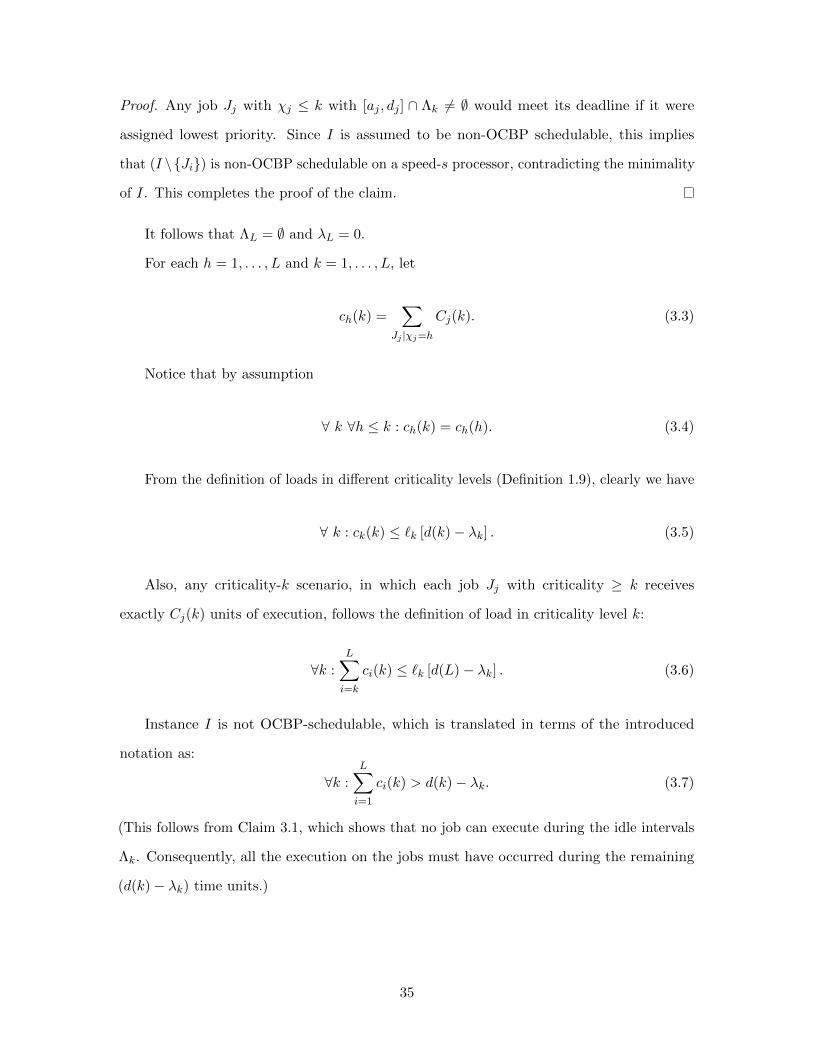
Proof. Any job Jj with χj ≤ k with [aj , dj ] ∩ Λk 6= ∅ would meet its deadline if it were

assigned lowest priority. Since I is assumed to be non-OCBP schedulable, this implies

that (I \{Ji}) is non-OCBP schedulable on a speed-s processor, contradicting the minimality

of I. This completes the proof of the claim.

It follows that ΛL = ∅ and λL = 0.

For each h = 1, . . . , L and k = 1, . . . , L, let

ch(k) =∑

Jj |χj=h

Cj(k). (3.3)

Notice that by assumption

∀ k ∀h ≤ k : ch(k) = ch(h). (3.4)

From the definition of loads in different criticality levels (Definition 1.9), clearly we have

∀ k : ck(k) ≤ `k [d(k)− λk] . (3.5)

Also, any criticality-k scenario, in which each job Jj with criticality ≥ k receives

exactly Cj(k) units of execution, follows the definition of load in criticality level k:

∀k :L∑i=k

ci(k) ≤ `k [d(L)− λk] . (3.6)

Instance I is not OCBP-schedulable, which is translated in terms of the introduced

notation as:

∀k :

L∑i=1

ci(k) > d(k)− λk. (3.7)

(This follows from Claim 3.1, which shows that no job can execute during the idle intervals

Λk. Consequently, all the execution on the jobs must have occurred during the remaining

(d(k)− λk) time units.)

35

Hence, for each k,

d(k)− λk <k−1∑i=1

ci(k) +L∑i=k

ci(k)

=k−1∑i=1

ci(i) +L∑i=k

ci(k) (by (3.4))

≤k−1∑i=1

`i [d(i)− λi] + `k [d(L)− λk] (by (3.5) and (3.6))

≤k−1∑i=1

`i [d(i)− λi] + `kd(L).

(3.8)

Therefore, for all k = 1, . . . , L,

d(k)− λk < `kd(L) +k−1∑i=1

`i [d(i)− λi] . (3.9)

Using notation δk = d(k)− λk (hence δL = d(L) since λL = 0) this yields

δk < `kδL +

k−1∑i=1

`iδi (3.10)

According to Condition 3.10, the summation part in (3.10) can be expanded recursively:

k∑i=1

`iδi

=`kδk +k−1∑i=1

`iδi

<`k

(`kδL +

k−1∑i=1

`iδi

)+k−1∑i=1

`iδi

(by (3.10))

=`2kδL + (`k + 1)k−1∑i=1

`iδi

(3.11)

By Condition 3.11, we can represent δL by only the loads iteratively:

36

δL <`LδL +L−1∑i=1

`iδi

<`LδL + `2L−1δL + (`L−1 + 1)L−2∑i=1

`iδi

(by (3.11))

<`LδL + `2L−1δL + (`L−1 + 1)`2L−2δL + (`L−1 + 1)(`L−2 + 1)L−3∑i=1

`iδi

(by (3.11) again)

· · ·

<`LδL +L−1∑k=h

`2kδL · L−1∏j=k+1

(`j + 1)

+L−1∏j=h

(`j + 1) ·h−1∑i=1

`iδi

· · ·

<`LδL +

L−1∑k=2

`2kδL · L−1∏j=k+1

(`j + 1)

+

L−1∏j=2

(`j + 1) · `1δ1

<`LδL +

L−1∑k=2

`2kδL · L−1∏j=k+1

(`j + 1)

+L−1∏j=2

(`j + 1) · `21δL

(by (3.8), δ1 < `1δL )

=`LδL +

L−1∑k=1

`2kδL · L−1∏j=k+1

(`j + 1)

(3.12)

If we divide both sides of Condition 3.12 by δL, we will get exactly

`L +L−1∑k=1

`2k · L−1∏j=k+1

(`j + 1)

> 1. (3.13)

This is to say, if I is not OCBP-schedulable and all the latest-deadline jobs in I are

of criticality L, the reverse form of Condition 3.1 holds, which concludes the proof that

Condition 3.1 is sufficient to OCBP-schedulability.

37

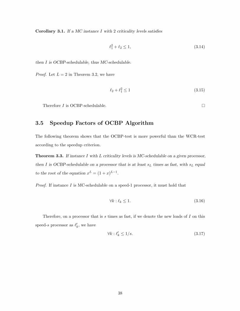
Corollary 3.1. If a MC instance I with 2 criticality levels satisfies

`21 + `2 ≤ 1, (3.14)

then I is OCBP-schedulable, thus MC-schedulable.

Proof. Let L = 2 in Theorem 3.2, we have

`2 + `21 ≤ 1 (3.15)

Therefore I is OCBP-schedulable.

3.5 Speedup Factors of OCBP Algorithm

The following theorem shows that the OCBP-test is more powerful than the WCR-test

according to the speedup criterion.

Theorem 3.3. If instance I with L criticality levels is MC-schedulable on a given processor,

then I is OCBP-schedulable on a processor that is at least sL times as fast, with sL equal

to the root of the equation xL = (1 + x)L−1.

Proof. If instance I is MC-schedulable on a speed-1 processor, it must hold that

∀k : `k ≤ 1. (3.16)

Therefore, on a processor that is s times as fast, if we denote the new loads of I on this

speed-s processor as `′k, we have

∀k : `′k ≤ 1/s. (3.17)

38

We notice that the l.h.s. of Condition 3.1 has no negative terms. Therefore, the l.h.s.

increases when any `k increases. Therefore on the speed-s processor,

`′L +L−1∑k=1

`′2k · L−1∏j=k+1

(`′j + 1)

≤1

s+L−1∑k=1

[1

s2·(

1

s+ 1

)L−k−1](by (3.17))

=1

s+

1

s2·L−2∑i=0

(1

s+ 1

)i=

1

s+

1

s2

[s2(1s + 1

)Ls+ 1

− s

]

=1

s+

(1s + 1

)Ls+ 1

− 1

s

=

(1s + 1

)Ls+ 1

=(1 + s)L−1

sL.

(3.18)

If s ≥ sL, we will have (1 + s)L−1 < sL. Thus the l.h.s. of Condition 3.1 will be no more

than 1. By Theorem 3.2, the instance I is schedulable on the speed-s processor.

Theorem 3.4. The speedup factor of sL is tight.

Proof. We now show that the factor sL is tight by giving instances with L criticality levels

that are MC-schedulable on a unit-speed processor, but not OCBP-schedulable on a processor

that is less than sL times as fast.

Consider the following instance consisting of 2L− 1 jobs:

� J1 = (0, d1 = σ1 = 1, 1, (

L times︷ ︸︸ ︷1, 1, . . . , 1)).

� For each i, 2 ≤ i ≤ L, there are two jobs:

– J2(i−1) = (0, σi−1, i, (

(i−1) times︷ ︸︸ ︷0, 0, . . . , 0 , σi−1, . . . , σi−1︸ ︷︷ ︸

L−(i−1) times

))

– J2i−1 = (0, σi, i, (σi − σi−1, . . . , σi − σi−1︸ ︷︷ ︸L times

)), where σi > σi−1.

39

This instance is MC-schedulable by the following policy. Assign greatest priority to the

jobs J2i in reverse order of their indices: J2L, J2(L−1), . . . , J2. Consider the scenario in which

c2h > 0, h ≥ 1, and c2j = 0, j > h. Then we execute J2h, J2h+1, J2h+3, . . . , J2L+1 in this

order; it is evident that each of them completes by its deadline.

For job J2h−1, h = 1, . . . , L to be assigned lowest priority in an OCBP-schedule, we

would need a speedup factor s of the processor such that

(σL − σL−1) + (σL−1 − σL−2) + · · ·+ (σ2 − σ1) + σ1 + (1 + σ2 + · · ·+ σj−1)

s=

σL + (1 + σ2 + · · ·+ σj−1)

s≤ σh.

Hence, for all h = 1, . . . , L, it requires

s ≥ σL + (1 + σ2 + · · ·+ σj−1)

σh.

Thus we have

s < minh=1,...,L

σL +∑h−1

i=1 σiσh

(3.19)

The minimum of the right hand side is maximized if all L terms are equal. Let x be this

maximum value. Then for all k = 1, . . . , L,

x =σL + σ1 + σ2 + · · ·+ σk−1

σk=xσk−1 + σk−1

σk=

(1 + x

σk

)σk−1.

Hence,

σk =(1 + x

x

)σk−1 ∀k = 1, . . . , L which implies σL =

(1 + x

x

)L−1σ1 .

Since, in particular, x = σLσ1

, we have

x =(1 + x

x

)L−1.

Therefore, s ≥ sL is necessary for OCBP algorithm to schedule this instance.

40

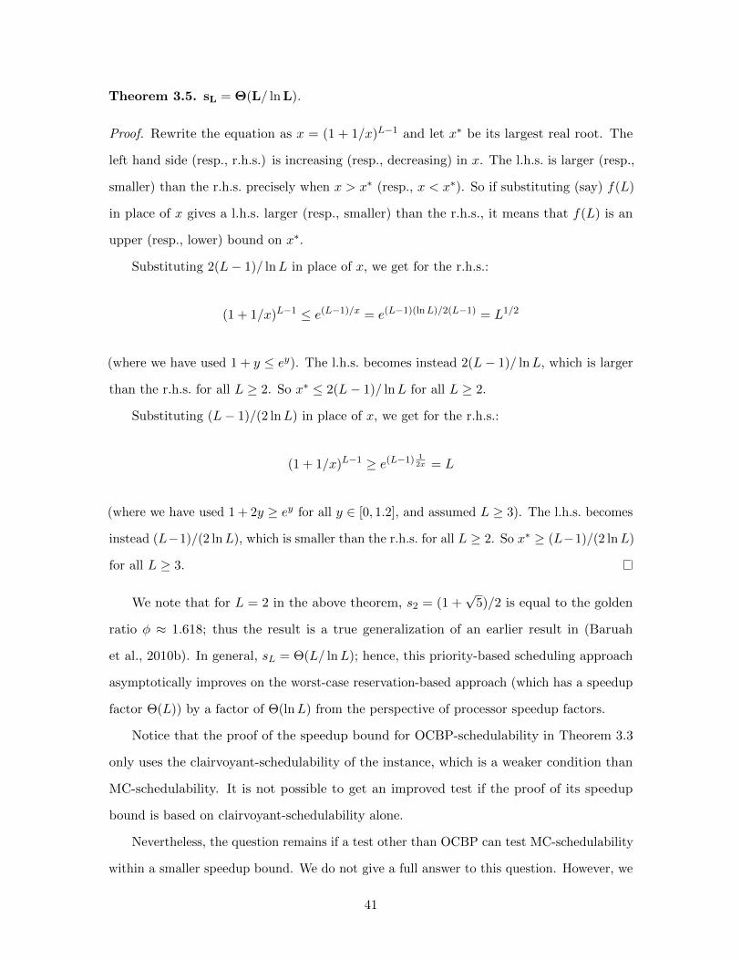
Theorem 3.5. sL = Θ(L/ ln L).

Proof. Rewrite the equation as x = (1 + 1/x)L−1 and let x∗ be its largest real root. The

left hand side (resp., r.h.s.) is increasing (resp., decreasing) in x. The l.h.s. is larger (resp.,

smaller) than the r.h.s. precisely when x > x∗ (resp., x < x∗). So if substituting (say) f(L)

in place of x gives a l.h.s. larger (resp., smaller) than the r.h.s., it means that f(L) is an

upper (resp., lower) bound on x∗.

Substituting 2(L− 1)/ lnL in place of x, we get for the r.h.s.:

(1 + 1/x)L−1 ≤ e(L−1)/x = e(L−1)(lnL)/2(L−1) = L1/2

(where we have used 1 + y ≤ ey). The l.h.s. becomes instead 2(L− 1)/ lnL, which is larger

than the r.h.s. for all L ≥ 2. So x∗ ≤ 2(L− 1)/ lnL for all L ≥ 2.

Substituting (L− 1)/(2 lnL) in place of x, we get for the r.h.s.:

(1 + 1/x)L−1 ≥ e(L−1)12x = L

(where we have used 1 + 2y ≥ ey for all y ∈ [0, 1.2], and assumed L ≥ 3). The l.h.s. becomes

instead (L−1)/(2 lnL), which is smaller than the r.h.s. for all L ≥ 2. So x∗ ≥ (L−1)/(2 lnL)

for all L ≥ 3.

We note that for L = 2 in the above theorem, s2 = (1 +√

5)/2 is equal to the golden

ratio φ ≈ 1.618; thus the result is a true generalization of an earlier result in (Baruah

et al., 2010b). In general, sL = Θ(L/ lnL); hence, this priority-based scheduling approach

asymptotically improves on the worst-case reservation-based approach (which has a speedup

factor Θ(L)) by a factor of Θ(lnL) from the perspective of processor speedup factors.

Notice that the proof of the speedup bound for OCBP-schedulability in Theorem 3.3

only uses the clairvoyant-schedulability of the instance, which is a weaker condition than

MC-schedulability. It is not possible to get an improved test if the proof of its speedup

bound is based on clairvoyant-schedulability alone.

Nevertheless, the question remains if a test other than OCBP can test MC-schedulability

within a smaller speedup bound. We do not give a full answer to this question. However, we

41

can rule out fixed-priority policies, that is, policies which execute the jobs in some ordering

fixed before execution. This ordering is not adapted during execution, except that we do not

execute jobs of criticality level i < h after a scenario was revealed to be a level-h scenario.

Such a policy admits a simple representation as a sequence of jobs and we say that an

instance I is Π-schedulable if there exists an ordering of jobs Π that is feasible for any

non-erroneous scenario.

The following result shows that OCBP is best possible among fixed-priority policies.

Theorem 3.6. There exist instances with L criticality levels that are clairvoyantly-schedulable,

but that are not Π-schedulable for any fixed-priority policy Π on a processor that is less

than sL times as fast, with sL being the root of the equation xL = (1 + x)L−1.

Proof. Consider an instance with L criticality levels and L jobs:

J1 : (0, 1, 1, (

L times︷ ︸︸ ︷1, 1, . . . , 1)),

and, for each i = 2, . . . , L,

Ji : (0, σi, i, (

i−1 times︷ ︸︸ ︷σi − σi−1, . . . , σi − σi−1,

L−i+1 times︷ ︸︸ ︷σi, . . . , σi )),

where σi will be specified later and satisfies σi−1 < σi.

For L = 3 we have the following example:

J1 : (0, 1, 1, (1, 1, 1))

J2 : (0, σ2, 2, (σ2 − 1, σ2, σ2))

J3 : (0, σ3, 3, (σ3 − σ2, σ3 − σ2, σ3)).

The system is clairvoyantly schedulable as, for each scenario of level i and for each job Jj ,

j ≥ i,∑j

k=iCk(i) = σj . It follows that a schedule that executes job Ji in the interval [0, σi]

and each job Jj , j > i, in the interval [σj−1, σj ] is feasible.

42

We now show that the system is Π-schedulable for a speed-s machine only if s ≥ sL

where sL is the positive real-valued solution of the equation

xL = (x+ 1)L−1.

Each fixed-priority work-conserving policy is a sequence of jobs. Let us consider a

sequence where the last scheduled job is Ji and a level i scenario. In this case the overall

execution time is∑L

j=1Cj(i) = σL +∑i−1

j=1 σj . Hence the schedule is feasible for a speed-s

machine if and only if:

sσi ≥ σL +

i−1∑j=1

σj .

By using the same arguments for each possible schedule, it follows that a fixed-priority policy

Π system is correct for a speed-s machine if and only if

s ≥ min1≤i≤L

{σL +

∑i−1j=1 σj

σi

}.

As we showed in the proof of Theorem 3.4, sL is the maximum value of s′ satisfying the

inequality:

min1≤i≤L

{σL +

∑i−1j=1 σj

σi

}≥ s′,

hence the system is Π-schedulable for a speed-s machine if and only if s ≥ sL.

The following result shows that OCBP has the best speedup factor among all scheduling

policies for instances with 2 criticality levels.

Theorem 3.7. There exist instances with 2 criticality levels that are clairvoyantly-schedulable,

but that are not Π-schedulable for any on-line scheduling policy Π on a processor that is

less than (1 +√

5)/2 times as fast.

Proof. Consider an instance with L criticality levels and L jobs (φ = (1 +√

5)/2):

J1 : (0, 1, 1, (1, 1))

J2 : (0, φ, 2, (φ− 1, φ))

43

The system is clairvoyantly schedulable because (1) in each scenario of criticality level

1, a clairvoyantly scheduling policy will execute J1 first, guarantee J1 receives 1 time unit

in the interval [0, 1], and guarantee J2 receives φ− 1 time unit in the interval [1, φ]; (2) in

each scenario of criticality level 2, a clairvoyantly scheduling policy will only execute J2 and

guarantee J2 receives φ time unit in the interval [0, φ].

We now show that the system is Π-schedulable for a speed-s machine only if s ≥ φ.

Because the behavior of the scenario is revealed only at run-time, we assume that in a

scenario, J1 will require at least 1 time unit and J2 will require at least φ− 1 time units.

Before J2 signals its completion, it is not clear whether the scenario is in criticality level 1

or criticality level 2.

Now we check the time instant when J2 receives exactly φ− 1 time units by Π on the

speed-s machine. If the time instant is earlier than 1, we will let J2 signal its completion. In

this case, the scenario is revealed to be criticality 1 and J1 must also receive 1 time unit in

time interval [0, 1]. Therefore, we have [(φ− 1) + 1]/s ≤ 1, which leads to s ≥ φ. Otherwise

if the time instant is later than 1, we will not let J2 signals its completion and reveal that

J2 will actually require φ time units. Because J2 still needs 1 time unit to complete in the

remaining time interval, we know that 1/s ≤ φ− 1, which also leads to s ≥ φ.

Therefore, any on-line scheduling policy Π will require at least a speed-φ processor to

correctly schedule this instance. This completes the proof.

3.6 Summary

In this chapter, we focus on the problem of scheduling mixed-criticality jobs. Compared

with the mixed-criticality sporadic task sets that we are going to discuss, mixed-criticality

job instances consist of finite jobs and certain release-times and deadlines, which make this

problem an important base case on which we build the theory of scheduling mixed-criticality

sporadic tasks. Also, the problem is interesting in theory because of its intractability in

the sense of strong NP-hardness. Therefore, we need to answer two questions: what is the

solution to this problem, and how good the solution is.

44

The first solution that we discuss in this chapter is worst-case reservation scheduling,

which is extended from the traditional methods in a straightforward way. The WCR-

approach regards all mixed-criticality jobs as traditional real-time jobs. Therefore this

approach doesn’t have a good performance in the sense of speedup factor because it fails to

take advantages of the characteristics of mixed-criticality systems.

The main solution that we discuss is the OCBP algorithm, which provides an applicable

solution to the mixed-criticality scheduling problem. We show that OCBP algorithm is

sufficient (always providing a correct scheduler) and efficient (always running in polynomial

time). The priority-based approach makes this algorithm easy to implement.

A large portion of this chapter focuses on “how approximate OCBP algorithm is”. The

primary analytic tool we use to answer the question is loads. Theorem 3.2 plays the most

important role in the analysis. This theorem is a highly generalized conclusion that can

provide quantitative load bounds for a specific number of criticality levels. It also leads

to Theorem 3.3 that gives speedup factors for a specific number of criticality levels. It

is very important to notice that all these load bounds and speedup factors are aimed at

evaluating OCBP algorithm instead of presenting schedulability tests — OCBP algorithm

itself is a good schedulability test. Load bounds and speedup factors are used to compare

OCBP algorithm and other algorithms (in this chapter it is the WCR-scheduling algorithm)

explicitly and quantitatively. Theorem 3.3 and 3.5 show directly that OCBP algorithm is

superior to WCR-scheduling algorithm. Theorem 3.6 and 3.7 show that OCBP algorithm is

superior than many other potential scheduling algorithms (including all other algorithms

in two-criticality-level case). Therefore, as a conclusion, OCBP algorithm has very good

performance in the sense of approximation.

45

CHAPTER 4

Scheduling Mixed-CriticalityImplicit-Deadline Tasks

In this chapter, we discuss the scheduling of mixed-criticality implicit-deadline tasks

with EDF-VD algorithm. The schedulability test and scheduling policy will be described in

Section 4.2 and 4.3. The quantitative properties, especially the speedup factor of EDF-VD

algorithm, will be discussed in Section 4.4 and 4.5.

4.1 An Overview of Algorithm EDF-VD

In this chapter, we focus on an important special case of sporadic task systems in which

each task τi satisfies the property that Di = Ti — such systems, as defined in Subsection

1.3.4, are called implicit-deadline, or Liu & Layland task systems(Liu and Layland, 1973).

Moreover, we focus on the dual-criticality case, which means the criticality levels will be no

more than 2.1 The preemptive uniprocessor scheduling of mixed-criticality implicit-deadline

sporadic task systems was studied in (Baruah et al., 2011a). An algorithm called EDF-VD

was proposed that has the same speedup guarantee as above — any task system that can

scheduled by an optimal clairvoyant algorithm on a given processor can be scheduled by

EDF-VD on a processor that is (1 +√

5)/2 times as fast. Moreover, the schedulability test of

EDF-VD has polynomial run-time complexity, and the run-time complexity per scheduling

decision was logarithmic in the number of tasks. Based on these run-time properties it is

evident that EDF-VD, in contrast to the algorithms in (Li and Baruah, 2010a; Guan et al.,

2011), can be considered suitable for implementation in actual systems.

1As mentioned in Section 1.3.3, we use the notation level lo and hi in this chapter.

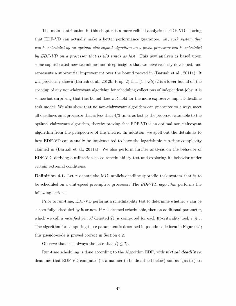
The main contribution in this chapter is a more refined analysis of EDF-VD showing

that EDF-VD can actually make a better performance guarantee: any task system that

can be scheduled by an optimal clairvoyant algorithm on a given processor can be scheduled

by EDF-VD on a processor that is 4/3 times as fast . This new analysis is based upon

some sophisticated new techniques and deep insights that we have recently developed, and

represents a substantial improvement over the bound proved in (Baruah et al., 2011a). It

was previously shown (Baruah et al., 2012b, Prop. 2) that (1+√

5)/2 is a lower bound on the

speedup of any non-clairvoyant algorithm for scheduling collections of independent jobs; it is

somewhat surprising that this bound does not hold for the more expressive implicit-deadline

task model. We also show that no non-clairvoyant algorithm can guarantee to always meet

all deadlines on a processor that is less than 4/3 times as fast as the processor available to the

optimal clairvoyant algorithm, thereby proving that EDF-VD is an optimal non-clairvoyant

algorithm from the perspective of this metric. In addition, we spell out the details as to

how EDF-VD can actually be implemented to have the logarithmic run-time complexity

claimed in (Baruah et al., 2011a). We also perform further analysis on the behavior of

EDF-VD, deriving a utilization-based schedulability test and exploring its behavior under

certain extremal conditions.

Definition 4.1. Let τ denote the MC implicit-deadline sporadic task system that is to

be scheduled on a unit-speed preemptive processor. The EDF-VD algorithm performs the

following actions:

Prior to run-time, EDF-VD performs a schedulability test to determine whether τ can be

successfully scheduled by it or not. If τ is deemed schedulable, then an additional parameter,

which we call a modified period denoted Ti, is computed for each hi-criticality task τi ∈ τ .

The algorithm for computing these parameters is described in pseudo-code form in Figure 4.1;

this pseudo-code is proved correct in Section 4.2.

Observe that it is always the case that Ti ≤ Ti.

Run-time scheduling is done according to the Algorithm EDF, with virtual deadlines:

deadlines that EDF-VD computes (in a manner to be described below) and assigns to jobs

47

Task system τ = {τ1, τ2, . . . τn} to be scheduled on a unit-speed preemptive processor.

1. Compute x as follows:

x← U2(1)

1− U1(1)

2. If(xU1(1) + U2(2) ≤ 1

)then

Ti ← xTi for each hi-criticality task τi

declare success and return

else declare failure and return

Figure 4.1: EDF-VD: The preprocessing phase.

before handing them off to the EDF scheduler. The EDF scheduler will then use these

virtual deadlines for the purpose of determining scheduling priority.

These virtual deadlines are assigned as follows. Suppose that a job of task τi arrives at

time-instant ta:

� If χi = lo, then this job is assigned a virtual deadline equal to ta + Ti.

� If χi = hi, then this job is assigned a virtual deadline equal to ta + Ti.

If some job does execute beyond its lo-criticality WCET without signaling that it has

completed execution, the following changes occur:

1. All currently-active lo-criticality jobs are immediately discarded; henceforth, no

lo-criticality job will receive any execution.

2. Subsequent run-time scheduling of the hi-criticality tasks (including their jobs that are

currently active) continue to be done according to EDF. But the actual job deadlines

(arrival time plus period) are used.

4.2 Schedulability Test: Pre-Runtime Processing

We now provide a detailed description of the pre-runtime processing conducted by EDF-

VD. We describe, and prove correct, the strategy used to determine whether a system

48

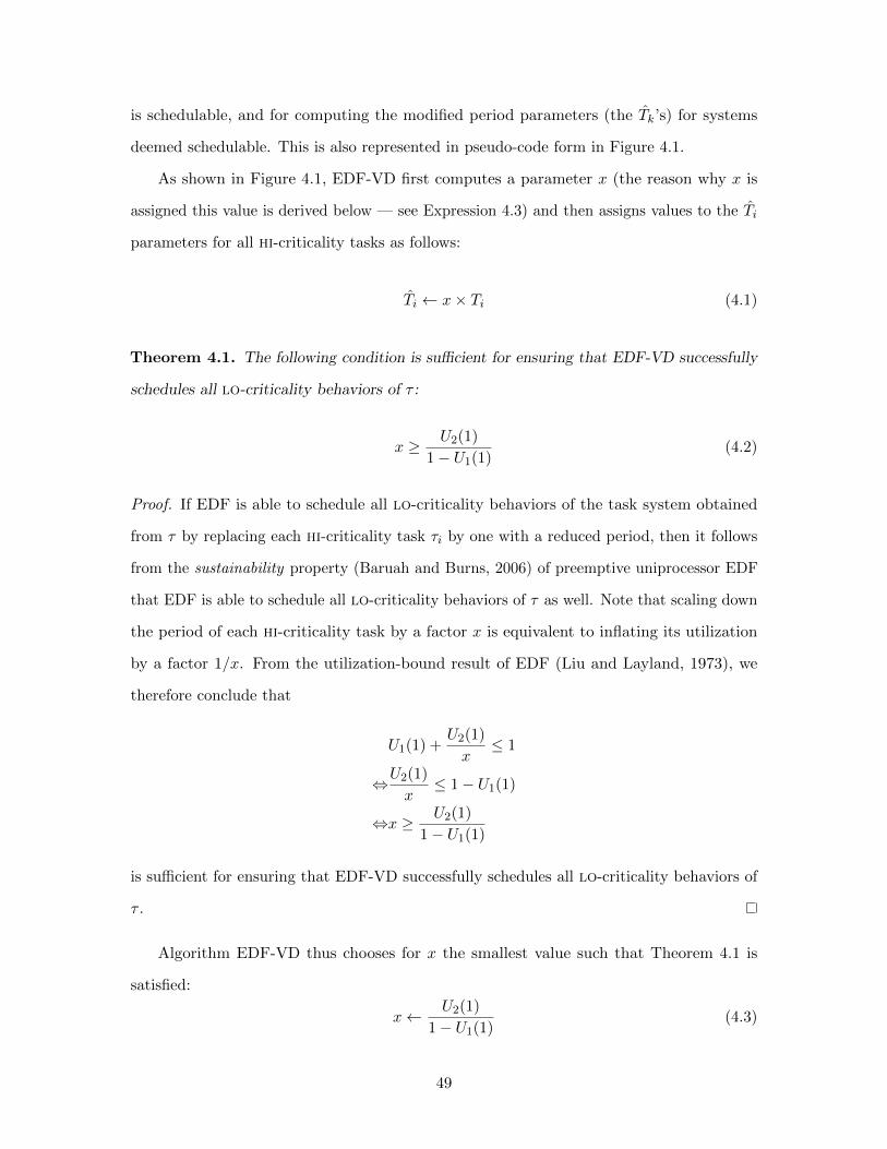
is schedulable, and for computing the modified period parameters (the Tk’s) for systems

deemed schedulable. This is also represented in pseudo-code form in Figure 4.1.

As shown in Figure 4.1, EDF-VD first computes a parameter x (the reason why x is

assigned this value is derived below — see Expression 4.3) and then assigns values to the Ti

parameters for all hi-criticality tasks as follows:

Ti ← x× Ti (4.1)

Theorem 4.1. The following condition is sufficient for ensuring that EDF-VD successfully

schedules all lo-criticality behaviors of τ :

x ≥ U2(1)

1− U1(1)(4.2)

Proof. If EDF is able to schedule all lo-criticality behaviors of the task system obtained

from τ by replacing each hi-criticality task τi by one with a reduced period, then it follows

from the sustainability property (Baruah and Burns, 2006) of preemptive uniprocessor EDF

that EDF is able to schedule all lo-criticality behaviors of τ as well. Note that scaling down

the period of each hi-criticality task by a factor x is equivalent to inflating its utilization

by a factor 1/x. From the utilization-bound result of EDF (Liu and Layland, 1973), we

therefore conclude that

U1(1) +U2(1)

x≤ 1

⇔U2(1)

x≤ 1− U1(1)

⇔x ≥ U2(1)

1− U1(1)

is sufficient for ensuring that EDF-VD successfully schedules all lo-criticality behaviors of

τ .

Algorithm EDF-VD thus chooses for x the smallest value such that Theorem 4.1 is

satisfied:

x← U2(1)

1− U1(1)(4.3)

49

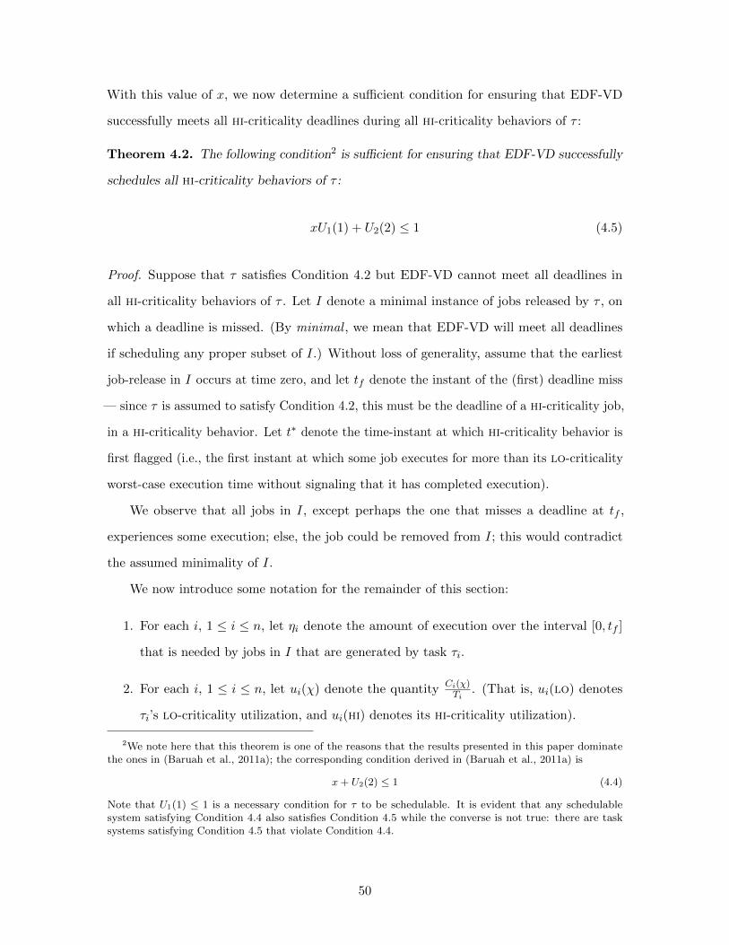
With this value of x, we now determine a sufficient condition for ensuring that EDF-VD

successfully meets all hi-criticality deadlines during all hi-criticality behaviors of τ :

Theorem 4.2. The following condition2 is sufficient for ensuring that EDF-VD successfully

schedules all hi-criticality behaviors of τ :

xU1(1) + U2(2) ≤ 1 (4.5)

Proof. Suppose that τ satisfies Condition 4.2 but EDF-VD cannot meet all deadlines in

all hi-criticality behaviors of τ . Let I denote a minimal instance of jobs released by τ , on

which a deadline is missed. (By minimal , we mean that EDF-VD will meet all deadlines

if scheduling any proper subset of I.) Without loss of generality, assume that the earliest

job-release in I occurs at time zero, and let tf denote the instant of the (first) deadline miss

— since τ is assumed to satisfy Condition 4.2, this must be the deadline of a hi-criticality job,

in a hi-criticality behavior. Let t∗ denote the time-instant at which hi-criticality behavior is

first flagged (i.e., the first instant at which some job executes for more than its lo-criticality

worst-case execution time without signaling that it has completed execution).

We observe that all jobs in I, except perhaps the one that misses a deadline at tf ,

experiences some execution; else, the job could be removed from I; this would contradict

the assumed minimality of I.

We now introduce some notation for the remainder of this section:

1. For each i, 1 ≤ i ≤ n, let ηi denote the amount of execution over the interval [0, tf ]

that is needed by jobs in I that are generated by task τi.

2. For each i, 1 ≤ i ≤ n, let ui(χ) denote the quantity Ci(χ)Ti

. (That is, ui(lo) denotes

τi’s lo-criticality utilization, and ui(hi) denotes its hi-criticality utilization).

2We note here that this theorem is one of the reasons that the results presented in this paper dominatethe ones in (Baruah et al., 2011a); the corresponding condition derived in (Baruah et al., 2011a) is

x+ U2(2) ≤ 1 (4.4)

Note that U1(1) ≤ 1 is a necessary condition for τ to be schedulable. It is evident that any schedulablesystem satisfying Condition 4.4 also satisfies Condition 4.5 while the converse is not true: there are tasksystems satisfying Condition 4.5 that violate Condition 4.4.

50

3. Let J1 denote the job with the earliest release time amongst all those that execute in

[t∗, tf ). Let a1 denote its release time, and d1 its deadline.

Claim 4.1. All jobs that execute in [t∗, tf ) have deadline ≤ tf .

Proof. Suppose not. Consider the latest instant t′ in [t∗, tf ) when a job with deadline > tf

executes. Only those jobs in I that have release time ≥ t′ and deadline ≤ tf are sufficient to

cause a deadline miss; this contradicts the assumed minimality of I.

Claim 4.2. Any lo-criticality task τi has

ηi ≤ ui(lo)(a1 + x(tf − a1)

)(4.6)

Proof. No lo-criticality job will execute after t∗. For it to execute after a1, it must have

a deadline no larger than J1’s virtual deadline, which is (a1 + x(d1 − a1)). Therefore, no

lo-criticality job with deadline > (a1 + x(tf − a1)) will execute after a1.

Suppose that some lo-criticality job with deadline > (a1 + x(tf − a1)) were to execute,

at some time < a1. Let t′ denote the latest instant at which any such job executes. This

means that at this instant, there were no jobs with effective deadline ≤ (a1 + x(tf − a1))

awaiting execution. Hence the instance obtained by considering only those jobs in I that

have release times ≥ t′ also misses a deadline; this contradicts the assumed minimality of

I.

Claim 4.3. Any hi-criticality task τi has

ηi ≤ui(lo)

xa1 + (tf − a1)ui(hi) (4.7)

Proof. We consider separately the cases when τi does not have a job with release time ≥ a1,

and when it does.

Case: If τi does not release a job at or after a1. We claim that each job of τi has a modified

deadline ≤ (a1 + x(tf − a1)). To see why this is so, consider some job with a modified

deadline > (a1 + x(tf − a1)), and let t′ denote the latest instant at which this job executes.

51

All jobs in I that have release times ≥ t′ also miss a deadline; this contradicts the assumed

minimality of I.

Since each job has a modified deadline ≤ (a1 + x(tf − a1)), their actual deadlines are all

≤ a1x + (tf − a1). Therefore, their cumulative execution requirement is at most

a1xui(lo) + (tf − a1)ui(lo)

≤ a1xui(lo) + (tf − a1)ui(hi)

Case: If τi releases a job at or after a1. Let ai denote the first release ≥ a1. The cumulative

execution requirement of all jobs of τi is at most

aiui(lo) + (tf − ai)ui(hi)

≤ a1ui(lo) + (tf − a1)ui(hi)

(since a1 ≤ ai and ui(lo) ≤ ui(hi))

≤ a1xui(lo) + (tf − a1)ui(hi)

(since x ≤ 1)

Thus in both cases, Condition 4.7 holds.

Let us sum the cumulative demand of all the tasks over [0, tf ):

∑χi=lo

ηi +∑χi=hi

ηi

≤∑χi=lo

ui(lo)(a1 + x(tf − a1)

)+∑χi=hi

a1xui(lo) + (tf − a1)ui(hi)

= a1(U1(1) +

U2(1)

x

)+(tf − a1)(xU1(1) + U2(2))

≤ (By choice of x [Eqn. 4.2], (U1(1) + U2(1)x ) ≤ 1)

a1 + (tf − a1)(xU1(1) + U2(2))

52

It follows from the infeasibility of this instance that

a1 + (tf − a1)(xU1(1) + U2(2)) > tf

⇔ (tf − a1)(xU1(1) + U2(2)) > tf − a1

⇔ xU1(1) + U2(2) > 1

Taking the contrapositive, it follows that (xU1(1) + U2(2) ≤ 1) is sufficient to ensure

hi-criticality schedulability by EDF-VD, as is claimed in this theorem.

We have thus established the correctness of Algorithm EDF-VD: by Theorem 4.1 the

value assigned to x ensures the correctness of all lo-criticality behaviors whereas Theorem 4.2

guarantees the correct scheduling of all hi-criticality behaviors.

Observation. Note that Theorem 4.1 requires that x ≥ U2(1)1−U1(1)

, while Theorem 4.2 requires

that x ≤ 1−U2(2)U1(1)

. When these upper and lower bounds on x are not equal to each other, a

pragmatic choice would be to choose a value for x that lies somewhere within the interval

(e.g., at the mid-point), rather than at either of the boundaries — this would increase the

robustness of the algorithm and its tolerance to, e.g., any arrival jitter.

4.3 Run-time Scheduling Policy

During the execution of the system, jobs are selected for execution according to the following

rules:

1. There is a criticality level indicator Γ, initialized to lo.

2. While (Γ ≡ lo),

(a) Suppose a job of some task τi ∈ τ arrives at time t

� if χi ≡ lo, the job is assigned a scheduling deadline equal to t+ Ti.

� if χi ≡ hi, the job is assigned a scheduling deadline equal to t+ Ti.

(b) At each instant the waiting job with earliest scheduling deadline is selected for

execution (ties broken arbitrarily).

53

(c) If the currently-executing job executes for more than its lo-criticality WCET

without signaling completion, then the behavior of the system is no longer a

lo-criticality behavior, and Γ← hi.

3. Once (Γ ≡ hi),

(a) The scheduling deadline of each hi-criticality job that is currently active is changed

to its release time plus the unmodified period parameter (the Ti, not the Ti) of

the task that generated it. That is, if a job of τi that was released at some time t

is active, its deadline, for scheduling purposes, is henceforth t+ Ti.

(b) When a future job of τi arrives at some time t, it is assigned a scheduling deadline

equal to t+ Ti.

(c) lo-criticality jobs will not receive any further execution. Therefore at each instant

the earliest-deadline waiting job generated by a hi-criticality task is selected for

execution(ties broken arbitrarily).

4. An additional rule could specify the circumstances when Γ gets reset to lo. This could

happen, for instance, if no hi-criticality jobs are active at some instant in time. (We

will not discuss the process of resetting Γ← lo any further in this document, since this

is not relevant to the certification process — lo-criticality certification assumes that

the system never exhibits any hi-criticality behavior, while hi-criticality certification

is not interested in the behavior of the lo-criticality tasks.)

4.3.1 An Efficient Implementation of Run-Rime Dispatching

For traditional (non-MC) sporadic task systems consisting of n tasks, uniprocessor EDF

can be implemented efficiently to have a run-time complexity of O(log n) per event, where

an event is either the arrival of a job, or the completion of the execution of a job (see,

e.g., (Mok, 1988)). A direct application of such implementations can be used to obtain an

implementation of the run-time dispatching of EDF-VD that has a run-time of O(log n) per

job-arrival and job-completion event. However, EDF-VD potentially needs to deal with an

additional run-time event: the change in the criticality level of the behavior from lo to hi

54

(this is the event that is triggered at the instant that Γ gets assigned the value hi). Since

this event requires that each subsequent scheduling be done according to each hi-criticality

task’s original deadline, explicitly recomputing priorities according to these original deadlines

would take time linear in the number of hi-criticality tasks — in the worst case, O(n) time.

We now describe an implementation of EDF-VD’s run-time system that has a worst-case

run-time of O(log n) per event for all three kinds of events: job arrival, job completion, and

change in the criticality level of the behavior from lo to hi.

Recall that a priority queue supports the operations of inserting (“insert”) and deleting

the smallest item (“deleteMin”) in logarithmic time, and the operation of finding the smallest

item (“min”) in constant time. In addition, the standard priority queue data structure

can be enhanced to support the deletion of a specified item (the “delete” operation), also

in logarithmic time (see, e.g, (Cormen et al., 2009, Sec. 6.5)). We maintain two such

enhance priority queues, Qlo and Qhi. We also use a timer that is used to indicate whether

the currently-executing job has executed for more than its lo-criticality WCET (thereby

triggering the assignment Γ← hi).

Initially, Γ ≡ lo and there are three kinds of events to be dealt with: (1) the arrival of

a job; (2) the completion of a job; and (3) Γ being assigned the value hi. We consider each

separately, below. Suppose that the event occurs at time-instant tc, and let Jc denote the

currently-executing job.

1. A job of task τi arrives at time tc.

(a) Insert the newly-arrived job into Qlo, prioritized according to its modified schedul-

ing deadline.

(b) If χi = hi (i.e., if it is a hi-criticality job), then also insert it into Qhi, prioritized

according to its unmodified (i.e., actual) scheduling deadline.

(c) If Jc is no longer the minimum job in Qlo, it must be the case that the newly-

arrived job has an earlier modified deadline than Jc’s modified deadline. In

that case, the newly-inserted job becomes Jc, and the timer is set to go off at

tc + Ci(lo) (when this newly-inserted job would exceed its lo-criticality WCET

if allowed to execute without interruption).

55

2. The currently-executing job Jc completes execution at time tc.

(a) Delete this job from Qlo, using the deleteMin operation supported by priority

queue implementations.

(b) If it was a hi-criticality job, also delete it from Qhi — this would be accomplished

by a delete operation.

(c) Set the current-job indicator Jc to denote the new minimum (modified) deadline

job — the “minimum” job in Qlo; and set the timer to go off at tc+ this job’s

remaining lo-criticality WCET (when the job would exceed its lo-criticality

WCET if allowed to execute without interruption).

3. The timer goes off, indicating that the currently-executing job has executed beyond

its lo-criticality WCET without signaling completion. The system is therefore now

in hi-criticality mode, and we switch to scheduling according to Qhi. Henceforth, all

run-time dispatch decisions are taken as indicated by this priority queue.

After Γ becomes hi, no lo-criticality jobs need execute, and hi-criticality jobs are executed

according to EDF with their original (unmodified) deadlines. Hence subsequent run-time

dispatching is done as for traditional EDF scheduling (as described in, e.g., (Mok, 1988)),

with Qhi being the priority queue used for this purpose.

4.4 Some Properties of EDF-VD Algorithm

In this section, we discuss two properties of EDF-VD algorithm. The first property is that

EDF-VD algorithm is strictly superior than WCR-scheduling algorithm; the second property

is that EDF-VD algorithm successfully schedules a boundary case where U2(1) = 0.

4.4.1 Comparison with Worst-Case Reservation Scheduling

Under the worst-case reservations strategy that is widely used in the design of mixed-

criticality systems, computing capacity is provisioned to each task at its own criticality level.

56

That is, the MC task system τ is mapped on to the traditional (non-MC) task system

⋃τi∈τ

{(Ci(χi), Ti

)}

and scheduled using regular EDF. It directly follows from the utilization-bound result of

EDF (Liu and Layland, 1973) that the condition

U1(1) + U2(2) ≤ 1 (4.8)

is necessary and sufficient for ensuring that EDF can schedule τ to meet all deadlines,

provided each lo-criticality job executes for up to its lo-criticality WCET and each hi-

criticality job executes for up to its hi-criticality WCET. This covers all lo-criticality and

all hi-criticality behaviors of τ .

We now show that Algorithm EDF-VD strictly dominates the worst-case reservations

approach: any task system that can be scheduled using worst-case reservations can be

scheduled by EDF-VD.

Theorem 4.3. Any task system τ that is correctly scheduled using worst-case reservations

is also correctly scheduled by EDF-VD.

Proof. Any task system that can be scheduled using worst-case reservations satisfies Condi-

tion 4.8 above.

U1(1) + U2(2) ≤ 1

⇒ (Since U2(1) ≤ U2(2))

U1(1) + U2(1) ≤ 1

⇒ U2(1)

1− U1(1)≤ 1

From this and Equation 4.3, we conclude that x is assigned a value ≤ 1 by Algorithm

EDF-VD.

57

Now, Theorem 4.2 contains the following sufficient condition for EDF-VD schedulability:

xU1(1) + U2(2) ≤ 1 ,

which always holds since Condition 4.8 holds and x ≤ 1.

4.4.2 Task Systems τ with U2(1) = 0

It is interesting to analyze the manner in which EDF-VD deals with task systems in which

the lo-criticality WCET of each hi-criticality task is equal to zero. (This would be the case

for systems in which a “mode change” can be thought to occur when the high-criticality

behavior is triggered.)

For such a system τ , observe that U2(1) = 0. Therefore, the value assigned to the scaling

parameter x in Step 1 of Figure 4.1 is equal to zero, and the test in Step 2 of Figure 4.1

evaluates to true to all τ with U2(2) ≤ 1. Thus EDF-VD can schedule any task system for

which U2(1) = 0 that satisfies the condition

U1(1) ≤ 1 and U2(2) ≤ 1 .

I.e., EDF-VD can schedule any such system provided the lo-criticality and the hi-criticality

behaviors are separately schedulable.

Continuing to analyze the pseudo-code in Figure 4.1 for this special case, we observe

that EDF-VD assigns each hi-criticality task τi a modified period Ti equal to zero. Thus

during run-time each job of a hi-criticality task immediately becomes an earliest-deadline

(and hence highest-priority) one upon arrival. If it is discovered to have a non-zero execution

time, the criticality-level indicator is immediately assigned the value hi (i.e., Γ← hi), and

all lo-criticality jobs are immediately discarded.

58

4.5 Speedup Factor of EDF-VD Algorithm

The speedup factor of an algorithm A for scheduling mixed-criticality systems is defined to be

the smallest real number f such that any task system τ that is schedulable on a unit-speed

processor by a hypothetical optimal clairvoyant algorithm is successfully scheduled on a

speed-f processor by algorithm A. The speedup factor is a convenient metric for comparing

the worst-case behavior of different algorithms for solving the same problem: the smaller

the speedup factor, the closer the behavior of the algorithm to that of a clairvoyant optimal

algorithm.

Theorem 4.4. The speedup factor of EDF-VD is ≤ 43 .

Proof. To prove this theorem, we will show that any MC implicit-deadline sporadic task

system that is clairvoyantly schedulable on a speed-34 processor is schedulable by EDF-VD

on a unit-speed processor.

Let b denote an upper bound on both the lo-criticality utilization and the hi-criticality

utilization of task system τ :

b ≥ max(U1(1) + U2(1), U2(2)

)(4.9)

By Theorems 4.1 and 4.2, we know that if an x satisfying both theorems exists, there will

be no deadline miss. Since Theorem 4.1 requires that

U2(1)

1− U1(1)≤ x

while Theorem 4.2 requires that

x ≤ 1− U2(2)

U1(1),

59

we can derive Expression 4.10 below as a sufficient condition for τ to be successfully scheduled

using EDF-VD:

U2(1)

1− U1(1)≤ 1− U2(2)

U1(1)

⇐ (Since U1(1) + U2(1) ≤ b⇒ U2(1) ≤ b− U1(1))

b− U1(1)

1− U1(1)≤ 1− U2(2)

U1(1)

⇐ (Since U2(2) ≤ b)b− U1(1)

1− U1(1)≤ 1− bU1(1)

⇔ (U1(1)

)2 − U1(1) + (1− b) ≥ 0 (4.10)

Now if we set b← 34 , Expression 4.10 becomes

(U1(1)

)2 − U1(1) +1

4≥ 0

⇔ (U1(1)− 1

2

)2 ≥ 0

which is true for all values of U1(1).

We have thus shown that any task system that is clairvoyant schedulable on a speed-34

processor is scheduled by EDF-VD to meet all deadlines on a unit-speed processor. It

therefore follows that any task system that is clairvoyant schedulable on a unit-speed

processor is scheduled by EDF-VD to meet all deadlines on a speed-43 processor, as claimed

by this theorem.

We now show that EDF-VD is optimal with regard to speedup factor:

Theorem 4.5. No non-clairvoyant algorithm for scheduling dual-criticality implicit-deadline

sporadic task systems can have a speedup bound better than 43 .

Proof. Consider the example task system τ = {τ1, τ2}, with the following parameters, where

ε is an arbitrarily small number > 0:

60

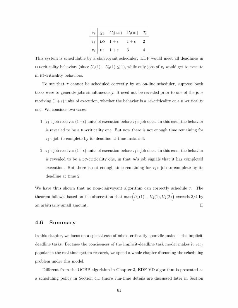
τi χi Ci(lo) Ci(hi) Ti

τ1 lo 1 + ε 1 + ε 2

τ2 hi 1 + ε 3 4

This system is schedulable by a clairvoyant scheduler: EDF would meet all deadlines in

lo-criticality behaviors (since U1(1) +U2(1) ≤ 1), while only jobs of τ2 would get to execute

in hi-criticality behaviors.

To see that τ cannot be scheduled correctly by an on-line scheduler, suppose both

tasks were to generate jobs simultaneously. It need not be revealed prior to one of the jobs

receiving (1 + ε) units of execution, whether the behavior is a lo-criticality or a hi-criticality

one. We consider two cases.

1. τ1’s job receives (1+ε) units of execution before τ2’s job does. In this case, the behavior

is revealed to be a hi-criticality one. But now there is not enough time remaining for

τ2’s job to complete by its deadline at time-instant 4.

2. τ2’s job receives (1+ε) units of execution before τ1’s job does. In this case, the behavior

is revealed to be a lo-criticality one, in that τ2’s job signals that it has completed

execution. But there is not enough time remaining for τ1’s job to complete by its

deadline at time 2.

We have thus shown that no non-clairvoyant algorithm can correctly schedule τ . The

theorem follows, based on the observation that max(U1(1) + U2(1), U2(2)

)exceeds 3/4 by

an arbitrarily small amount.

4.6 Summary

In this chapter, we focus on a special case of mixed-criticality sporadic tasks — the implicit-

deadline tasks. Because the conciseness of the implicit-deadline task model makes it very

popular in the real-time system research, we spend a whole chapter discussing the scheduling

problem under this model.

Different from the OCBP algorithm in Chapter 3, EDF-VD algorithm is presented as

a scheduling policy in Section 4.1 (more run-time details are discussed later in Section

61

4.3). Therefore, we need to construct the schedulability test for this scheduling policy. In

Section 4.2, we describe and prove the schedulability condition in Figure 4.1. The proof

is done by considering the maximum time demand over a low-criticality or high-criticality

busy interval, while the time demand in the interval is shaped by utilizations. A possible

future work may exist because we actually simplified the problem by discarding specific task

parameters in the system. If we can bound the time demand by a more detailed description

with task parameters, we may get a more accurate schedulability condition. The current

result consists of only utilizations — it means that all sporadic task systems are equivalent

in the schedulability test if they have identical high/low utilizations.

The speedup factor for EDF-VD algorithm on mixed-criticality implicit-deadline sporadic

tasks is 4/3, which is better than the previously shown factor 1.618 (Baruah et al., 2011a).

Surprisingly, it is also better than OCBP algorithm’s 1.618 factor on mixed-criticality jobs

(which is shown to be optimal in two-criticality-level case). The reason is that implicit-

deadline model imports more constraints to the system, so we can shape the time demand

in an interval more accurately. We show that the 4/3 factor is optimal, which means that it

is impossible to discover any on-line scheduling algorithm that has a better speedup factor

(but it is possible to find a better algorithm that accepts more task sets that EDF-VD). As

a further contribution, we have shown how EDF-VD can be implemented to have a run-time

complexity per scheduling decision that is logarithmic in the number of tasks, and thus

demonstrated the practical applicability of the algorithm.

62

CHAPTER 5

Scheduling Mixed-CriticalityArbitrary-Deadline Tasks

In this chapter, we discuss the scheduling of mixed-criticality arbitrary-deadline tasks

with EDF-VD algorithm. Because the scheduling policy remains the same as in Chapter 4,

we focus on the schedulability test in Section 5.2, and on the speedup factor in 5.3.

5.1 Overview

Here we study the case in which deadlines do not equal periods, the so-called sporadic task

system with arbitrary deadlines. In this chapter we still only consider task systems that

consist of two criticality levels.

In the case that deadlines are not equal to periods, we need more than the notion of

utilization in order to determine schedulability. In classical real-time scheduling theory, the

load of an instance denotes the maximum over all time intervals, of the cumulative execution

requirement by jobs of the instance over the interval, normalized by the interval length.

Informally, the load of an instance represents a lower bound on the speed of any processor

upon which it can meet all deadlines.

As introduced in Section 1.3, a sporadic task system τ can generate infinitely many

different instances. Each instance can be seen as an independent collection of jobs where

the realized arrival time of job Jij of task τj is denoted by aij and its absolute deadline

by dij = aij + dj . Then for instance I of the mixed-criticality system we can define three

notions of load, analogous to the beforementioned concept from real-time scheduling.

The following definition defines the “worst-case load” of a mixed-criticality system, in

addition to the previously defined loads in different criticality levels:

Definition 5.1. The load `(I), the lo-load `1(I) and the hi-load `2(I) of a mixed-criticality

instance I with two criticality levels are defined according to the following three formulas:

`(I) = max0≤t1<t2

∑Jij :t1≤aij∧dij≤t2

cj(χj)

t2 − t1,

`1(I) = max0≤t1<t2

∑Jij :t1≤aij∧dij≤t2

cj(1)

t2 − t1,

`2(I) = max0≤t1<t2

∑Jij :χj=2∧t1≤aij∧dij≤t2

cj(2)

t2 − t1.

Informally, `(I) is the largest load the system can have if no job is omitted at all; `1(I)

is the largest load the system can have if we clairvoyantly know that the system runs in

lo-criticality level; `2(I) is the largest load the system can have if we clairvoyantly know

that the system runs in hi-criticality level.

These definitions extend in the obvious manner to systems of sporadic tasks. The load

of sporadic task system `(τ) is defined to be the largest value that `(I) can have, for any

instance I generated by τ . We define by the synchronous arrival sequence of task system τ

the collection of job arrivals in which each task generates a job at time-instant zero, and

subsequent jobs arrive as soon as possible. It is well-known (Baruah et al., 1990) that the

largest demand over any time interval is reached for this synchronous arrival sequence. Also,

note that only values of t1 and t2 have to be considered where t1 is equal to some aij and

t2 is equal to some dij . For the interval [0, lcm{c1, . . . , cn}), there are a pseudo-polynomial

number of such intervals [t1, t2).

Thus, for any task system τ , all three loads can be computed in pseudo-polynomial time

using well-known techniques for determining the loads of “regular” (i.e., non-MC) sporadic

task systems. Specifically, `(τ), `1 and `2 are respectively the loads of “regular” sporadic task

systems {(cj(χj), dj , cj) |τj ∈ τ}, {(cj(1), dj , cj) |τj ∈ τ} and {(cj(2), dj , cj) |τj ∈ τ ∧χj = 2}.

In the sequel we will abbreviate `(τ), `1(τ) and `2(τ) to `0, `1 and `2.

64

5.2 Schedulability Test

The following observation gives a necessary condition for any scheduling algorithm to schedule

an MC task system.

Claim 5.1. If for any MC task system τ , `1 > 1 or `2 > 1, the system is not schedulable by

any scheduling algorithm.

The relationship between the three loads is given in the next observation.

Claim 5.2. For any MC task system τ , `0 ≤ `1 + `2.

Algorithm EDF-VD: The EDF-VD algorithm proceeds as follows:

Case 1. If `0 ≤ 1, schedule all the jobs with EDF scheduler according to their original

deadlines;

Case 2. If `0 > 1, test if `1 + `2/2 ≤ 1 and (`1`2 − 2`1)2 − 4`1(`1 − `2 + `22) ≥ 0. If

both inequalities hold, set x = 1− `2/2, scale the relative deadlines of every hi-criticality

job Jij from task τj from dj to dj = xdj , and accordingly, the absolute deadlines from

dij = aij + dj to dij = aij + xdj . In lo-criticality level, schedule all the jobs with the EDF

scheduler according to the original deadlines of lo-criticality jobs and the virtual deadlines

of hi-criticality jobs; when the system’s behavior alters to hi (a hi-criticality job uses more

than its lo-criticality WCET), cancel all lo-criticality jobs, reset all hi-criticality jobs’

deadlines to the original ones, and schedule the hi-criticality jobs with EDF according to

their original deadlines immediately.

We prove that the EDF-VD algorithm is correct by the following three theorems.

Theorem 5.1. If an MC task system τ satisfies `0 ≤ 1, it is schedulable by EDF-VD.

Proof. Notice that if every job uses its maximum execution time, which means all lo-

criticality jobs use cj(1) and all hi-criticality jobs use cj(2), the load of the system will be

bounded by `0. Since EDF is the optimal scheduling strategy on a preemptive uniprocessor,

Case 1 of EDF-VD algorithm guarantees that the task system is schedulable if `0 ≤ 1.

65

Theorem 5.2. If an MC task system τ satisfies `1 ≤ 1, setting the scaling parameter x

in the EDF-VD algorithm such that `1 ≤ x ≤ 1, will guarantee that the system meets all

deadlines in lo-criticality behavior.

Proof. To prove that there is no deadline miss, we assume the opposite, which is that a job

J0 misses its deadline in lo-criticality behavior. Let I denote a minimal instance of jobs

released by τ on which a deadline is missed. The deadline of job J0 is denoted as d0. Now,

if we inspect the jobs that can block job J0 from execution (in the sense that they have

an earlier (virtual) deadline and are therefore given priority by EDF), it can only be the

lo-criticality jobs that have deadlines no greater than d0, and the hi-criticality jobs that

have virtual deadlines no greater than d0. Notice that all virtual deadlines can be represented

as dij = aij + xdj ≥ x(aij + dj) = xdij . If dij ≤ d0, the previous inequality leads to the

conclusion that all hi-criticality jobs that can block the execution of job J0 will have actual

absolute deadline no later than d0/x. Therefore, the cumulative execution requirement of

the system until time d0 is at most `1 · d0/x in lo-criticality behavior. Because J0 misses its

deadline d0, it must hold that

d0x`1 > d0

⇔ `1 > x. (5.1)

Since we assumed that job J0 missed its deadline in lo-criticality behavior, the contrapositive

of (5.1),

x ≥ `1, (5.2)

must be a sufficient condition for schedulability in lo-criticality level.

Theorem 5.3. If an MC task system τ satisfies (`1`2 − 2`1)2 − 4`1(`1 − `2 + `22) ≥ 0, then

by selecting x = 1− `2/2 as the scaling parameter in the EDF-VD algorithm, the system

will not miss any deadline in hi-criticality behavior.

66

Proof. To prove that there is no deadline miss, we argue by contradiction and assume that a

job J2 misses its deadline at time d2. Let I denote the minimal instance in which a deadline

miss occurs. Therefore, job J2 must be of hi-criticality. Denote by time t∗ the time instant

that hi-criticality behavior is first flagged.

Claim 5.3. All jobs Jij that are executed in [t∗, d2), have actual absolute deadline dij ≤ d2,

where d2 is the deadline of the job that misses its deadline.

Proof. Note that only jobs of hi-criticality level will execute after t∗. Further, after t∗ the

original deadlines of all jobs are restored. Now suppose there is a job that has a deadline

larger than d2, but is executed somewhere in [t∗, d2) and let [t′, t′′) be the last interval in

which it was executed. That means that in that interval no jobs with deadlines smaller or

equal to d2 were pending. The instance obtained by only considering the jobs with release

time at least t′′ also misses a deadline and this contradicts the assumed minimality of I.

It is crucial to explicitly identify which jobs can block the execution of job J2. We have

seen from Fact 5.3 that all jobs that are executed after t∗ can block the execution of J2 (for

their hi-criticality execution time). We define the set of jobs which are executed after t∗ as

S2. From the definition J2 ∈ S2, and furthermore, the jobs in S2 (except J2 itself) are the

only jobs that can block the execution of J2 in hi-criticality. Thus in lo-criticality, the jobs

that block execution of jobs in S2 will consequently block the execution of J2.

Definition 5.2. Let t be the time instant when the first job in S2 is released. This job is

denoted as J1 and d1 is its actual absolute deadline.

By definition, we know that before time t, there are no jobs in S2 available. Thus J2 is

also released at or after t. And from Fact 5.3, all jobs in S2 have deadlines no later than d2,

which implies d1 ≤ d2.

In order to calculate the maximum possible execution requirement that blocks execution

of J2, we present the following lemma.

Lemma 5.1. Any job Jij that is in the minimal instance I and is able to block the execution

of J2 in lo-criticality behavior must have absolute deadline dij ≤ t + x(d2 − t) if it is a

lo-criticality job, and virtual absolute deadline dij ≤ t+ x(d2 − t) if it is a hi-criticality job.

67

Proof. Note that no lo-criticality job Jij with dij > d1 will execute at or after t. That

would mean that somewhere in the interval [t, t∗) there is no job with deadline at most d1

awaiting execution. This contradicts the fact that J1 is in S2 (and thus receives execution

after t∗) and hence is not finished before t∗.

Suppose there is a lo-criticality job Jij with dij > d1 that executes somewhere before

t. Denote by t′ the latest moment in time where it executes. At this point there are no

available jobs with deadline at most d1 and the instance obtained by only considering jobs

released after t′ also misses a deadline. That contradicts the assumed minimality of I.

So, any lo-criticality job Jij must have a deadline dij ≤ d1 = t+x(d1− t) ≤ t+x(d2− t),

where the last inequality comes from Fact 5.3.

Suppose that there is a hi-criticality job Jij with virtual deadline dij , that is released

at time aij ≤ t. Since its actual deadline is at most d2, its virtual deadline is at most

aij+x(d2−aij) and this is no more than t+x(d2−t). Hence, such a job has dij ≤ t+x(d2−t).

If its release time aij > t, the job can only receive execution in lo-criticality level if its

virtual deadline is at most the virtual deadline of J1. Hence, dij ≤ d1 = t + x(d1 − t) ≤

t+ x(d2 − t).

Now, similar to the concept of S2, we define the set of lo-criticality jobs that are able

to block execution of jobs in S2 (which includes J2) as S11 , and the set of hi-criticality jobs

that are only executed before t∗ and that are able to block the execution of jobs in S2 as S21 .

Definition 5.3. Let c11 be the sum of execution requirements of jobs in S11 ; c2 the sum of

execution requirements of jobs in S2; and let c21 be sum of execution requirements of jobs in

S21 .

Definition 5.4. Let d = d2 − t. This means that d is the length of the time interval where

jobs from S2 exist.

From Lemma 5.1, we directly get the following two inequalities

c11 ≤ `1(t+ xd)

c11 + c21 ≤ `1(t/x+ d).

(5.3)

68

The second inequality holds because aij + xdj = dij ≤ t+ xd gives that dj ≤ (t+ xd)/x,

similar to the conclusion we get in the proof of Theorem 5.2.

By definition of `2, we also obtain another set of inequalities

c2 ≤ `2d

c2 + c21 ≤ `2(t/x+ d).

(5.4)

Since J2 misses its deadline d2 = t+ d as we assumed, we have c11 + c21 + c2 > d2, which is

equivalent to c11 + c21 + c2 − t > d. This is to say, there exist certain d and t such that for

given L and x, c11 + c21 + c2 − t > d holds. Without loss of generality, we assume that d is

constant (since all other values can be scaled proportionally), then the maximum value of

c11 + c21 + c2 − t for all possible t will be greater than d.

In order to get the maximum value of our object function o(t) = c11 + c21 + c2 − t, from

inequalities (5.3) and (5.4), we get

o(t) ≤

f(t) = `1(t+ xd) + `2(t/x+ d)− t

g(t) = `1(t/x+ d) + `2d− t.(5.5)

Note that since `1 + `2 > 1 (otherwise it must be the case that `0 ≤ `1 + `2 ≤ 2×0.5 = 1,

according to Observation 5.2) and `1/x ≤ 1 (because of Theorem 5.2) We obtain the following

two inequalities

∂f(t)

∂t= `1 + `2/x− 1 ≥ `1 + `2 − 1 > 0

∂g(t)

∂t= `1/x− 1 ≤ 1− 1 = 0,

(5.6)

The inequalities in (5.6) show that when t increases, f(t) increases and g(t) decreases,

for t ∈ (0,+∞). Thus max [o(t)] can not exceed the intersection of f(t) and g(t), otherwise

at least either the inequalities in (5.3) or in (5.4) will be violated. We denote the value of t

where f(t) = g(t) as γ.

It is easy to find that

69

γ =`1(1− x)xd

`2 − `1(1− x), (5.7)

and therefore

max [o(t)] ≤ o(γ) =`22 + `1`2x− `1x+ `1x

2

`2 − `1 + `1xd (5.8)

That is to say, if J2 misses its deadline as we assumed, it must hold that o(γ) > d for

given `1, `2 and x. Or equivalently,

`1x2 + (`1`2 − 2`1)x+ `1 − `2 + `22 > 0. (5.9)

However, x is a value of our choice between (0, 1). We can select x = −(`1`2−2`1)/2`1 =

1− `2/2 ∈ (0, 1) to get the minimum value of the left side of inequality (5.9). If inequality

o(γ) > d must hold, we need to let

(`1`2 − 2`1)2 − 4`1(`1 − `2 + `22) < 0, (5.10)

so that o(γ) > d no matter what value we choose for x.

Finally we reach our conclusion that if J2 misses its deadline for certain t and d as

we assumed, we must have inequality (5.10) to hold to assure that o(γ) ≥ max [o(t)] > d.

Because we assumed that a job would miss its deadline in hi-criticality behavior, the

contrapositive of (5.10),

(`1`2 − 2`1)2 − 4`1(`1 − `2 + `22) ≥ 0 (5.11)

is sufficient to guarantee no deadline miss in hi-criticality level if we select x = 1− `2/2.

70

Theorem 5.4. If for any MC task system τ , `1+`2/2 ≤ 1 and (`1`2−2`1)2−4`1(`1−`2+`22) ≥

0, the system is schedulable by the EDF-VD algorithm.

Proof. By Theorem 5.3, we can select x = 1 − `2/2 to guarantee no deadline miss in hi-

criticality level. By Theorem 5.2, x = 1 − `2/2 ≤ `1 can guarantee no deadline miss in

lo-criticality level.

Theorem 5.5. If for any MC task system τ , `0 ≤ 1 or max{`1, `2} ≤ 4− 2√

3, the system

is schedulable by the EDF-VD algorithm.

Proof. If `0 ≤ 1, by Theorem 5.1, the system is schedulable. Otherwise, we can assume

that L > 0.5(otherwise it must be the case that `0 ≤ L + L ≤ 2 × 0.5 = 1, according to

Observation 5.2). Now if we define the left side of (5.11) as L(`1, `2), it’s easy to verify that

∂L(`1, `2)

∂`1= 2`2[`1(`2 − 4)− 2`2 + 2] < 0

∂L(`1, `2)

∂`2= 2`1[`1(`2 − 2)− 4`2 + 2] < 0.

(5.12)

Therefore, if we define L = 4− 2√

3, the minimum value of L(`1, `2) is reached at (L,L).

Hence we have

L(`1, `2) ≥ L(L,L) = (L2 − 2L)2 − 4L3 = 0. (5.13)

Obviously `1 + `2/2 ≤ 1. By Theorem 5.4, the system is schedulable by EDF-VD

algorithm.

5.3 Speedup Factor Result

Theorem 5.6. If an MC task system τ is schedulable on a given processor, it is schedulable

by the EDF-VD algorithm on a processor that is 1 + 12

√3 ≈ 1.866 times faster.

71

Proof. If an MC task system τ is schedulable on a given processor, by Observation 5.1, `1

and `2 on the given processor are no greater than 1. Thus on the (1 + 12

√3)-speed processor,

its `′1(T ) and `′2(T ) are no greater than 1/(1 + 12

√3) = 4− 2

√3. By Theorem 5.5, this task

system is schedulable on the (1 + 12

√3)-speed processor.

Theorem 5.7. There exists a sporadic task system τ with `1 = `2 = 4 − 2√

3 + ε (with

ε > 0 arbitrarily small) which can not be scheduled by the EDF-VD algorithm.

Proof. Again, we define L = 4 − 2√

3, N is a very large positive integer and M is a very

large positive integer, even compared to N . We define a task system τ as follows (every task

is represented respectively as ([cj(1), cj(2)], dj , cj , χj))

T = {τ1 = ([L,L],1− ε, +∞, 1),

τ2 = ([0, L+ ε],1, +∞, 2),

τ31 = ([(√L− L)/N, (

√L− L)/N ],1 + (1/

√L− 1)/N, +∞, 2),

τ32 = ([(√L− L)/N, (

√L− L)/N ],1 + 2(1/

√L− 1)/N, +∞, 2),

· · · ,

τ3i = ([(√L− L)/N, (

√L− L)/N ],1 + i(1/

√L− 1)/N, +∞, 2),

· · · ,

τ3N = ([(√L− L)/N, (

√L− L)/N ],1/

√L, +∞, 2),

· · · ,

τ3M = ([(√L− L)/N, (

√L− L)/N ],1 +M(1/

√L− 1)/N, +∞, 2)}.

It is easy to verify that `1 and `2 of τ are both L+ ε, by considering the synchronous

arrival sequence, i.e., all tasks release a job at time 0 and subsequent job are release as soon

as permitted by the problem parameters. If we only consider τ1 and τ2, the claim is trivial.

If we take τ31 , τ32 , · · · , and τ3i into consideration, we can see the lo-criticality time demand

in time interval [0, 1 + i(1/√L− 1)/N) is

72

`1 ≥L+ i(

√L− L)/N

1 + i(1/√L− 1)/N

= L.

A similar inequality holds for `2. Therefore `1 and `2 of τ are both L+ ε.

Now let us assume that we have selected a scaling factor x. We would like to show that

the system is not schedulable with this (arbitrary) given x.

Given x, we assume that τ2 releases its first job at time 1− x, and all other tasks release

their first job at time 0 . Then, the actual deadline of the first job of τ2 (denoted as J2) is

d2 = 1− x+ 1 = 2− x, and the virtual deadline will be d′2 = (1− x) + x× 1 = 1. Because

the virtual deadline is greater than the deadline of the first job of τ1 (denoted as J1), which

is d1 = 1− ε, J2 will wait until J1 finishes.

Also, we would like to know how many jobs in the set S3 = {τ31 , · · · , τ3i , · · · , τ3N , · · · , τ3M }

will execute before d2. If N is sufficiently large, we can represent the lo-criticality execution

requirement of S3 in time interval [0, t) where t ≥ 1 as Lt− L because we can always find

an i such that 1 + i(1/√L− 1)/N is sufficiently close to t, and we only have to subtract L

which is the WCET of J1.

We know that every job in S3 with xdi < d2 = 1 (i.e., di < 1/x) will be executed before

J2. As stated in previous paragraph, the execution requirement for this time interval [0, 1/x)

will be L/x− L.

Now let us calculate the execution requirement until time d2. It will be L + L +

ε + L/x − L = L + L/x + ε. Also, d2 = 2 − x as we computed. It is obvious that

L+L/x+ε−(2−x) = L+L/x+x−2+ε ≥ L+2√L−2 = 4−2

√3+2(

√3−1)−2+ε = ε > 0.

Hence, for this arbitrarily given x, we can always release the jobs carefully so that in the

time interval [0, 2− x), the execution requirement is greater than the length of the interval

(intuitively, smaller x will take more jobs in S3 into account, and larger x will reduce the

length of [0, 2 − x) which eventually causes a deadline miss, too). This implies that is is

impossible to schedule τ using the EDF-VD algorithm.

73

5.4 Summary

We explore the arbitrary-deadline sporadic task, which is a more generalized task model

in this chapter. The run-time scheduling policy keeps the same as in Chapter 4 — we

still use EDF-VD algorithm which applies virtual deadlines to high-criticality, while a new

schedulability test is applied to this new case. We maintain the idea for constructing the

schedulability test — considering the maximum time demand over a low-criticality or high-

criticality busy interval. The schedulability test becomes more complicated as the shaping

of time demands over an interval becomes harder by loads, compared with by utilizations.

The speedup factor for EDF-VD algorithm on mixed-criticality arbitrary-deadline tasks

is 1.866. We show that this factor is the best we can get for EDF-VD algorithm. No better

factor (with a low bound of 1.618 shown in Section 3.5) can be achieved unless the current

version of EDF-VD algorithm is modified or better algorithms are invented.

74

CHAPTER 6

Other Contributions

In this chapter, we briefly introduce other contributions including the extension of OCBP

algorithm on recurrent tasks and the extension of EDF-VD algorithm on multiprocessor

platforms.

6.1 OCBP Algorithm on Mixed-Criticality Recurrent Tasks

In Chapter 3, we considered the scheduling of mixed-criticality job instances: workloads that

are specified as collections of independent jobs rather than as systems of recurrent tasks.

Though OCBP is designed to work on mixed-criticality jobs, it can also be extended to

support mixed-criticality sporadic task systems.

The two main obstacles to apply OCBP algorithm to sporadic task systems are: (1) The

OCBP algorithm has two phases: an off-line phase during which priorities are computed

for all the jobs, followed by the run-time phase which deploys priority-based dispatching

using the priorities assigned during the off-line phase. But since any instance generated by a

sporadic task system may contain infinitely many jobs, the off-line procedure for computing

all the priorities prior to runtime is not guaranteed to terminate. (2) The algorithm for

determining OCBP priorities requires the complete specification of all the jobs in the instance.

However, under the (reasonable) assumption that our run-time scheduling algorithm is not

clairvoyant, we do not know this information beforehand for sporadic task systems: although

we may know a lower bound on the release times of jobs, a jobs exact release time only

becomes known when it is actually released.

We deal with the first of these problems — potentially infinitely many jobs — by only

assigning priorities, at each instant in time, to those jobs that arrive during the current

busy interval, where the busy interval refers to a maximal continuous interval of time during

which the processor is not idled. (This is reasonable: since OCBP scheduling never idles

the processor while there are jobs awaiting execution, scheduling decisions made within a

particular busy interval are not impacted by the priorities assigned to jobs arriving outside

that busy interval.) For any sporadic task system with all loads `k strictly less than one,

prior techniques from real-time scheduling theory can be applied to bound the maximum

length of the longest busy interval, and thereby determine the largest collection of jobs that

can possibly execute before the processor is idled.

Example 6.1. This example briefly shows the procedure to calculate the longest busy

interval for a dual-criticality sporadic task system τ . The loads `1 and `2 are the same as

defined in Definition 5.1. The technique can be plainly generalized to multiple criticality

level cases. We note that this is a pessimistic bound that is to show that such bounds exist,

rather than to compute the tightest bound. Less rough estimation can be obtained by more

advanced techniques (such as in (George et al., 1996; Ripoll et al., 1996)).

In OCBP algorithm, no lo-criticality job is executed once any job executes for more

than its lo-criticality WCET. Let us therefore consider the longest busy interval as being

comprised of two parts: (i) from the beginning of the busy interval up to the instant (if

any) at which some job executes for more than its lo-criticality WCET, and (ii) from that

instant to the end of the busy interval. Without loss of generality, we assume that the busy

interval starts at time-instant zero, some job executes for more than its lo-criticality WCET

at time-instant x1, and the busy interval ends at time-instant x1 + x2.

Let Dmax denote the largest deadline of any task in τ : Dmax = maxτi∈τ{Di}. All jobs

executed over [0, x1) have their release times and deadlines within the interval [0, x1 +Dmax);

hence

x1 ≤ `1(Dmax + x1) (6.1)

⇔ x1 ≤`1

1− `1×Dmax (6.2)

76

Since all jobs executing during [x1, x1 +x2) have their release times and deadlines within

the interval [0, x1 + x2 +Dmax, it must be the case that

x2 ≤ `2(x1 + x2 +Dmax)

⇔x2 ≤ `2(

`11− `1

×Dmax + x2 +Dmax

)(by (6.1))

⇔x2 ≤`2

(1− `1)(1− `2)×Dmax

(6.3)

The length of the longest busy interval is then bounded from above by x1 + x2. Under

the assumption that `1 and `2 are both bounded from above by a constant strictly less than

one, this is easily seen to be pseudopolynomial in the representation of τ . Once the length

of the longest busy period has been bounded as above, it is straightforward to bound which

jobs could have arrived within this interval — there will be at most pseudopolynomially

many such jobs.

To deal with the second problem — job release times (and hence deadlines) not known in

advance, we assign priorities under the assumption that all jobs in the current busy interval

are released as soon as legally permitted to do so under the constraints of the sporadic task

model. Actually, for the purposes of assigning the priorities, we can assume that all these

jobs are “early-released”, which means that they are immediately available in the beginning

of the busy interval. We don’t have to simulate the behavior of the schedule as we propose in

Section 3.3. If we represent a job collection in the longest busy interval of a mixed-criticality

system τ as I and assume that the busy interval starts at time t0, a job Jk ∈ Iτ can be

assigned the lowest priority if

∑∀i:Ji∈I

Ci(χk) ≤ (dk − t0) (6.4)

Identical to the method we described in Section 3.3, we include all jobs in the longest

busy interval in I in the beginning, and repeatedly apply the algorithm to the new collection

of jobs excluding the lowest priority job, until a full priority list is generated or the iteration

is terminated.

77

During runtime, we will monitor the actual job-release times; as long as they conform

to the ones we had used in assigning priorities, we need do nothing. When they do not

so conform, we will, under some circumstances, need to re-compute the priorities assigned

to some of the jobs. The only circumstances that need priority re-computation are: the

processor is idle, or the execution of some lesser-priority job Jx is preempted due to the

release of some greater-priority job Jy. We use the following dual-criticality example to

illustrate our method, which can be generalized to multiple criticality cases.

Example 6.2. A detailed dispatching procedure for a dual-criticality sporadic task system

can be described as follows: at each instant, the job Ji with the lowest priority that has

been released but not yet signalled completion is selected for execution. This continues until

one of the following events has occurred:

1. Some job Ji executes for more than ci(lo) without signalling that it has completed

execution. This implies that the system is now in hi-criticality mode, and hi-criticality

jobs are no longer required to complete by their deadlines. We may therefore discard

all lo-criticality jobs. It follows from the correctness of the OCBP priority assignment

at to that all hi-criticality jobs that will arrive during the current busy interval are

guaranteed to complete by their deadlines.

2. Under our priority-based scheduling model, the processor is idled at some time-instant

t only if all jobs that had arrived prior to t have completed execution by time-instant t.

If this happens, the current busy interval has ended, and priorities that were assigned

at t0 to jobs that ended up not arriving during this busy interval are “canceled”. We

await the release of some job, which will signal the start of a new busy interval — at

that time, we will recompute the priorities of all jobs that could possibly be scheduled

during that busy interval.

3. The execution of some lesser-priority job Jx is preempted due to the release of some

greater-priority job Jy, say at time-instant t1. We must recompute the priority list at

this point in time. It is proved that this recomputation can always generate a new

priority list (or equivalently, the schedule according to OCBP so far doesn’t make the

78

system unschedulable even though some tasks arrive late). We will not discuss the

detailed proof here.

The main theorem in this section is stated below:

Theorem 6.1. Given an MC sporadic task system τ , if the instance Iτ which consists of

the jobs in the longest busy interval of τ is OCBP-schedulable on a processor, then τ is

MC-schedulable (and thus schedulable) on the same processor.

This theorem shows that there is an algorithm that successfully schedules any mixed-

criticality sporadic task system whose longest busy interval is OCBP schedulable, or satisfies

the load condition described in Theorem 3.2. The algorithm has a pseudo-polynomial

time complexity in both pre-process and run-time stage, which is relatively computational-

expensive compared with EDF-VD algorithm in Chapter 5. However, the algorithm has

maintained the optimal speedup factor 1.618 in dual-criticality case, which is superior than

EDF-VD.

6.2 Multiprocessor Mixed-Criticality Scheduling

With the modernistic trend of implanting real-time systems on multiprocessor platforms,

it is of significance to discover the possibility of scheduling mixed-criticality systems on

multiprocessors. The EDF-VD algorithm is extended to both global multiprocessor scheduling

(tasks and jobs can migrate among processors) and partitioned multiprocessor scheduling

(tasks are assigned to dedicated processors).

6.2.1 Global Mixed-Criticality Scheduling

Our global mixed-criticality scheduling approach extends the EDF-VD uniprocessor mixed-

criticality scheduling algorithm to multiprocessors, by applying a previously-proposed multi-

processor global scheduling algorithm called fpEDF (Baruah, 2004), that was designed for

non mixed-criticality systems.

Algorithm fpEDF (Baruah, 2004) is a global EDF-based algorithm for scheduling systems

of non mixed-criticality implicit-deadline sporadic tasks upon identical multiprocessor

79

platforms. Suppose that “regular” (i.e., non-MC) implicit-deadline sporadic task system τ

is to be scheduled on m unit-speed processors. During run-time all jobs of tasks in τ that

have utilization greater than 1/2 are assigned highest priority, and the remaining tasks’ jobs

are assigned priorities according to their deadlines (as in “regular” EDF).

The following theorem is a corollary from Theorem 4 in (Baruah, 2004):

Theorem 6.2. If a task system cannot be scheduled by Algorithm fpEDF on m unit-speed

processors, then it cannot be scheduled by preemptive uniprocessor EDF on a processor of

speed (m+ 1)/2.

Now we provide a high-level overview of the global mixed-criticality scheduling algorithm.

Let τ = {τ1, . . . , τn} denote the MC implicit-deadline sporadic task system that is to be

scheduled on m unit-speed preemptive processors. Our approach to scheduling τ can be

thought of as a three-phased one.

During the pre-processing phase, a schedulability test is performed to determine whether

τ can be successfully scheduled by our algorithm or not. If τ is deemed schedulable, then

an additional parameter, which we call a modified period denoted Ti, is computed for each

hi-criticality task τi ∈ τ . We will see the details for the pre-processing phase later.that

Ti ≤ Ti.

Initial run-time scheduling is done according to previously described Algorithm fpEDF

(Baruah, 2004). Since fpEDF is defined for regular, rather than mixed-criticality, task systems,

we must map the mixed-criticality tasks in τ to regular tasks. This is done as follows: each lo-

criticality task τk = (χk, Ck(lo), Ck(hi), Tk) in τ is mapped to a regular implicit-deadline task

(Ck(lo), Tk), while each hi-criticality task τk = (χk, Ck(lo), Ck(hi), Tk) in τ is mapped to a

regular implicit-deadline task (Ck(lo), Tk), where the Tk’s are the modified periods computed

during the pre-processing phase. It follows from the sustainability property (Baruah and

Burns, 2006; Baker and Baruah, 2008) of Algorithm fpEDF that if Algorithm fpEDF is able

to schedule this regular implicit-deadline sporadic task system then it is able to schedule all

lo-criticality behaviors of the MC implicit-deadline task system τ .

80

If some job does execute beyond its lo-criticality WCET without signaling that it has

completed execution, we enter the third phase of the algorithm, and the following changes

occur.

1. All currently-active lo-criticality jobs are immediately discarded; henceforth, no

lo-criticality job will receive any execution.

2. Subsequent run-time scheduling of the hi-criticality tasks (including their jobs that

are currently active) are done according to Algorithm fpEDF. In order to do so, we

must once again map these hi-criticality tasks to regular implicit-deadline tasks. This

is done as follows: each hi-criticality MC task τk = (χk, Ck(lo), Ck(hi), Tk) in τ is

mapped to a regular implicit-deadline task (Ck(hi), Tk − Tk).

We now specify what happens during the pre-processing phase. The idea behind

our schedulability test (pre-processing phase) is to ensure that there is sufficient computing

capacity available between this time-instant t∗ and the deadline of each currently-active

hi-criticality job, to be able to execute all these jobs for up to their hi-criticality WCET’s

by their respective deadlines. This is ensured by the manner in which the modified periods

(the Tk parameters) are computed. We will compute modified period values to ensure that

the following two properties are satisfied:

1. All jobs of all tasks will meet their modified deadlines in any lo-criticality behavior

of the system (i.e., if no job executes beyond its lo-criticality WCET). That is, the

collection of “regular” (non-MC) tasks

( ⋃χi=lo

{(Ci(lo), Ti)

})⋃( ⋃χi=hi

{(Ci(lo), Ti)

})(6.5)

is scheduled by Algorithm fpEDF to always meet all deadlines on the available m

unit-speed processors.

2. If each hi-criticality job executes for no more than its hi-criticality WCET and each

lo-criticality job does not execute at all then each hi-criticality job can meet its

(original) deadline by beginning execution at or after its modified deadline. This is

81

ensured by ensuring that the collection of “regular” (non-MC) tasks

⋃χi=hi

{(Ci(hi), Ti − Ti)

}(6.6)

can be scheduled by Algorithm fpEDF to always meet all deadlines on the available m

unit-speed processors.

According to the description above, the pre-processing phase can be specified in pseudo-

code form in Figure 6.1. We provide an explanation of this pseudo-code below.

Step 1 checks to see whether Algorithm fpEDF can schedule the system if each lo-

criticality job executes for up to its lo-criticality WCET, and each hi-criticality job executes

for up to its hi-criticality WCET. If so, then the system can be scheduled directly by

Algorithm fpEDF; else, Steps 2-3 are executed.

In Step 2, a minimum “scaling factor” x is determined, such that if all the hi-criticality

tasks have their periods scaled by this factor x then the regular implicit-deadline task

system obtained by combining these tasks with the lo-criticality tasks would be successfully

scheduled by Algorithm fpEDF. The derivation of the value of x is as follows. According

to Theorem 6.2, Algorithm fpEDF can schedule any task system with total utilization

≤ (m+ 1)/2 (recall that m denotes the number of unit-speed processors). Since scaling the

period of each hi-criticality task by a factor x is equivalent to inflating its utilization by a

factor 1/x, for ensuring lo-criticality schedulability by fpEDF we therefore need

U1(1)(τ) +U2(1)(τ)

x≤ m+ 1

2

⇔U2(1)(τ)

x≤ m+ 1

2− U1(1)(τ)

⇔x ≥ U2(1)(τ)/(m+ 1

2− U1(1)(τ)

)This accounts for the first term in the “max”. The second term is to ensure that

scaling down the period of any hi-criticality task by this factor x does not result in the task

having its lo-criticality WCET exceed its scaled-down period (equivalently, the term Ci(lo)xTi

becoming > 1 for some hi-criticality task τi).

82

Task system τ = {τ1, τ2, . . . τn} to be scheduled on m processors.

1. If the regular task system ⋃i

{(Ci(χi), Ti)

}is deemed schedulable on the m processors by Algorithm fpEDF, then declare successand return.

2. x← max(U2(1)(τ)/

(m+12 − U1(1)(τ)

),maxχi=hi

{Ui(lo)

})3. If the regular task system ⋃

χi=hi

{(Ci(hi), (1− x)Ti)

}is deemed schedulable on the m processors by Algorithm fpEDF, then

Ti ← xTi for each hi-criticality task τi

declare success and return.

else declare failure and return.

Figure 6.1: Global EDF-VD: The preprocessing phase.

Step 3 determines whether the hi-criticality tasks can be scheduled to meet all deadlines

by Algorithm fpEDF once the behavior of the system transits to hi-criticality (i.e., after

the time-instant t∗ at which some job is identified to have executed for more than its

lo-criticality WCET). If so, the modified deadline parameters — the Ti’s — are computed.

In the end of this subsection, we state the following conclusions without proof, in order

to provide a quantitative way to evaluate the performance of our global mixed-criticality

scheduling method.

A following sufficient schedulability condition can be derived for our multiprocessor

mixed-criticality scheduling algorithm:

Theorem 6.3. Any task system τ satisfying

U1(1)(τ) + min(U2(2)(τ),

U2(1)(τ)

1− U2(2)(τ) · 2/(m+ 1)

)≤ m+ 1

2(6.7)

is successfully scheduled by our algorithm on m preemptive unit-speed processors.

A speedup factor bound is computed for the global EDF-VD scheduling algorithm:

83

Theorem 6.4. The processor speedup factor of the global EDF-VD scheduling algorithm is

no larger than (√

5 + 1). That is, any mixed-criticality task system that can be scheduled in

a certifiably correct manner on m unit-speed processors by an optimal clairvoyant scheduling

algorithm can be scheduled by our algorithm on m speed-(√

5 + 1)

processors.

6.2.2 Partitioned Mixed-Criticality Scheduling

The partitioned scheduling algorithm assigns each task to a dedicated processor, then

schedule all the tasks by EDF-VD algorithm on each processor. Therefore, we do not need

to discuss the scheduling policy here because it remains the same. We only describe the

partitioning algorithm, which has two phases:

1. During the first phase each hi-criticality task is assigned to some processor while

ensuring that the cumulative hi-criticality utilization assigned to each processor does

not exceed 3/4.

2. During the second phase each lo-criticality task is assigned to some processor while

ensuring that the cumulative lo-criticality utilization assigned to each processor also

does not exceed 3/4.

Observe that by Theorem 4.4, such an assignment procedure ensures that each processor

remains schedulable by EDF-VD. The algorithm reports failure if it fails to successfully

assign every task.

Now we provide a detailed description of our partitioned mixed-criticality scheduling

algorithm. Let τ denote the implicit-deadline sporadic task system that is to be partitioned

amongst m processors. Let us assume that there are n tasks in τ , of which n1 are hi-criticality

tasks. Without loss of generality, assume that τ1, τ2, . . . , τn1 are the hi-criticality tasks, and

τn1+1, . . . , τn the lo-criticality ones. Let π1, π2, . . . , πm denote the m processors. Let us

suppose that tasks τ1, τ2, . . . , τi−1 have been successfully assigned. We now explain how the

task τi is assigned to a processor.

For any processor πk, let τ(πk) denote the tasks from amongst τ1, τ2, . . . , τi−1 that have

already been assigned to it. Our algorithm assigns the task τi to any processor πk satisfying

84

the following condition. If i ≤ n1 (i.e., if τi is a hi-criticality task) then

Ui(hi) +∑

τj∈τ(πk)

Uj(hi)

≤ 3

4(6.8)

else (i.e., i > n1 and τi is hence a lo-criticality task)

Ui(lo) +∑

τj∈τ(πk)

Uj(lo)

≤ 3

4(6.9)

If no such πk exists, then the algorithm declares failure: it is unable to partition τ upon

the m-processor platform.

It can be easily proved that our algorithm provides a valid partition, which means after

the processor assignment, all processors are schedulable by EDF-VD after all tasks in τ have

been successfully assigned. We will not discuss the detailed proof here.

Also, a speedup factor bound is also calculated for the partitioned EDF-VD scheduling

algorithm:

Theorem 6.5. The speedup bound of the partitioned EDF-VD scheduling algorhim on an

m-processor platform is (8m− 4)/3m, which asymptotically approaching 8/3 as m→∞.

The partitioning algorithm appears to be better, from the perspective of speedup bounds,

when compared to the global algorithm. However, because neither of these two speedup

factors are proved to be tight, we will not claim the supremacy of the partitioning scheduling

algorithm.

85

CHAPTER 7

Conclusion

7.1 A Summary of Research Results

Due to the rapid increase in the complexity and diversity of functionalities that are performed

by safety-critical embedded systems, the cost and complexity of obtaining certification for

such systems is fast becoming a serious concern. We believe that in mixed-criticality sys-

tems, these certification considerations give rise to fundamental new resource allocation

and scheduling challenges which are not adequately addressed by conventional real-time

scheduling theory. In this dissertation, we focus on a mixed-criticality model that is particu-

larly designed for representing mixed-criticality workloads. We derive several scheduling

algorithms, including OCBP algorithm for scheduling mixed-criticality jobs, and EDF-VD

algorithm for scheduling implicit-deadline and arbitrary-deadline mixed-criticality sporadic

tasks. We conduct a thorough investigation of the schedulability properties of these algo-

rithms, including quantitative load bounds on these scheduling algorithms, and quantitative

performance guarantees according to the speedup factors.

OCBP algorithm is an ideal scheduling algorithm for mixed-criticality jobs. It is very

efficient in the sense of both run-time complexities and computational resource utilizations.

Based on priorities, the OCBP schedulability test and the OCBP run-time dispatcher are

both easy to implement. We have shown the speedup factors of OCBP algorithm for arbitrary

numbers of criticality levels. We also show that the speedup factors are lower (hence better)

than the traditional WCR-scheduling algorithm. It is very impressive to note that OCBP

algorithm has the best speedup factors in all fixed-job-priority scheduling policies, and

more impressively, the best speedup factor 1.618 in all on-line scheduling policies for two

criticality levels. It keeps an open question how good OCBP algorithm is if compared to an

optimal (and provably in exponential time assuming P6=NP) on-line scheduling algorithm. In

order to answer that question, we need more exploration to discover the essence of optimal

on-line scheduling algorithms. Current results only show the comparison of OCBP algorithm

with clairvoyant algorithms which can assure that no computational resource is wasted

but is impractical in reality. Also, it keeps an open question what is the best possible

speedup factors in all on-line scheduling policies for arbitrary numbers of criticality levels,

and consequently, whether there is an algorithm that achieves these factors.

EDF-VD algorithm is also an ideal scheduling algorithm for dual-criticality implicit-

deadline sporadic tasks. The criteria of selecting jobs for execution (seeking the job with

the earliest virtual deadline) is very effective for indefinite job releases. We also show that

EDF-VD algorithm has a speedup factor of 4/3, which implies that EDF-VD algorithm

always utilizes no less than 75% of the computational resources. Also, this is the best speedup

factors in all online scheduling policies for two criticality levels and implicit-deadline tasks.

It is not surprising to see that implicit-deadline mixed-criticality tasks can be scheduled

with less resource wastes than mixed-criticality jobs and arbitrary-deadline tasks, because

the conciseness of implicit-deadline tasks brings in more predictability — the same as in

the non-mixed-criticality case. In fact, the hardness of scheduling mixed-criticality implicit-

deadline tasks remains an open problem since the NP-hardness proof of MC-schedulability

problem (Baruah et al., 2010c, 2012b) can not be applied to implicit-deadline case.

The choice of algorithm for scheduling mixed-criticality arbitrary-deadline sporadic tasks

is more difficult to make. Both OCBP algorithm and EDF-VD algorithm can be extended

to the arbitrary-deadline case. The OCBP algorithm for sporadic tasks keeps the speedup

factors of OCBP algorithm, including the optimal speedup factor 1.618 for dual-criticality

case. However, because the scheduling policy needs to alter the priorities of the jobs in

run-time, the run-time complexity appears high. On the other hand, the EDF-VD algorithm

for sporadic tasks keeps the low run-time complexity of the scheduling policy. As a trade-off,

the computational resource waste is higher than OCBP algorithm, and so far only the

dual-criticality case is solved by EDF-VD algorithm.

The multiprocessor mixed-criticality scheduling algorithms in this dissertation are

designed based on EDF-VD algorithm for dual-criticality implicit-deadline sporadic systems.

87

As an initial effort, we show that this problem can be solved in both global and partitioned

ways. The speedup factors, 3.236 for global mixed-criticality scheduling and 2.67 for

partitioned mixed-criticality scheduling are shown to be neither optimal nor tight. Therefore,

we expect to provide some intuitions to work on and we expect to see improved results based

on our current progress.

7.2 Future Plan

Mixed-criticality scheduling research will be foreseeably attractive for a long time. After

answering the fundamental questions in mixed-criticality scheduling theory, we can still

perceive the vast blank in this area. Firstly, it is noticeable that the scheduling policies for

recurrent tasks on uniprocessor platforms are swaying among approximation ratio (OCBP

algorithm for sporadic tasks) and run-time complexity (EDF-VD algorithm for sporadic

tasks), while the comprehensive methods that excel at both are limited to two criticality

levels and implicit-deadline cases(EDF-VD algorithm for implicit-deadline sporadic tasks).

The existence of the supreme uniprocessor scheduling policy remains an open question.

Secondly, the scheduling theory on multiprocessor platforms is still incomplete because of

the lack of optimality proofs and the restriction of task types, processor types and migration

rules. Further research is required for the boundary of the performance of multiprocessor

mixed-criticality scheduling algorithms for various task types (implicit-/arbitrary-deadline)

on various processor types (identical/heterogeneous/unrelated) with various migration rules

(unrestricted/job level/task level). Finally, the scheduling theory with dependency constraints

(task dependency/resource sharing/hierarchical scheduling) is undeveloped. I would like to

work on these problems and complete the mixed-criticality scheduling theory.

Besides the scheduling theory which only gives an abstract overview of the real-time

systems, practice is always needed so that complex details of the real-world systems would be

covered. The theoretical guarantee of the temporal correctness requires a flawless interaction

between the schedulers and the other parts of the safety-critical embedded systems. In

order to completely deliver the theoretical guarantees, it is necessary to look into the role of

schedulers in such systems by studying the design and implementation of these systems, and

88

provide applicable scheduling components so that the temporal correctness will be seamlessly

integrated in these systems. To meet this goal, issues like system architectures, component

communications and run-time environments must be considered, and the awareness of

possible failures must be established. We shall never be too confident in how to build

accurate models and how to reasonably apply theoretical results to the practical systems.

The importance of the connection between theory and practice shall never be underestimated.

89

BIBLIOGRAPHY

Audsley, N. C. (1991). Optimal priority assignment and feasibility of static priority taskswith arbitrary start times. Technical report, The University of York, England.

Audsley, N. C. (1993). Flexible Scheduling in Hard-Real-Time Systems. PhD thesis, Depart-ment of Computer Science, University of York.

Baker, T. and Baruah, S. (2008). Sustainable multiprocessor scheduling of sporadic tasksystems. In Proceedings of the EuroMicro Conference on Real-Time Systems, Dublin.IEEE Computer Society Press.

Baruah, S. (2004). Optimal utilization bounds for the fixed-priority scheduling of periodictask systems on identical multiprocessors. IEEE Transactions on Computers, 53(6).

Baruah, S., Bonifaci, V., D’Angelo, G., Li, H., Marchetti-Spaccamela, A., van der Ster, S.,and Stougie, L. (2012a). The preemptive uniprocessor scheduling of mixed-criticalityimplicit-deadline sporadic task systems. In Proceedings of the 2012 24th EuromicroConference on Real-Time Systems, ECRTS ’12, Pisa (Italy). IEEE Computer Society.

Baruah, S., Bonifaci, V., D’Angelo, G., Marchetti-Spaccamela, A., van der Ster, S., andStougie, L. (2011a). Mixed-criticality scheduling of sporadic task systems. In Proceedingsof the 19th Annual European Symposium on Algorithms, pages 555–566, Saarbrucken,Germany. Springer-Verlag.

Baruah, S. and Burns, A. (2006). Sustainable scheduling analysis. In Proceedings of theIEEE Real-time Systems Symposium, pages 159–168, Rio de Janeiro. IEEE ComputerSociety Press.

Baruah, S., Burns, A., and Davis, R. (2011b). Response-time analysis for mixed criticalitysystems. In Proceedings of the IEEE Real-Time Systems Symposium (RTSS), Vienna,Austria. IEEE Computer Society Press.

Baruah, S. and Fohler, G. (2011). Certification-cognizant time-triggered scheduling ofmixed-criticality systems. In Proceedings of the IEEE Real-Time Systems Symposium(RTSS), Vienna, Austria. IEEE Computer Society Press.

Baruah, S. and Haritsa, J. (1997). Scheduling for overload in real-time systems. IEEETransactions on Computers, 46(9):1034–1039.

Baruah, S., Li, H., and Stougie, L. (2010a). Mixed-criticality scheduling: improved resource-augmentation results. In Proceedings of the ICSA International Conference on Comput-ers and their Applications (CATA). IEEE.

Baruah, S., Li, H., and Stougie, L. (2010b). Towards the design of certifiable mixed-criticalitysystems. In Proceedings of the IEEE Real-Time Technology and Applications Symposium(RTAS). IEEE.

Baruah, S., Mok, A., and Rosier, L. (1990). Preemptively scheduling hard-real-time sporadictasks on one processor. In Proceedings of the 11th Real-Time Systems Symposium, pages182–190, Orlando, Florida. IEEE Computer Society Press.

90

Baruah, S. and Vestal, S. (2008). Schedulability analysis of sporadic tasks with multiplecriticality specifications. In Proceedings of the EuroMicro Conference on Real-TimeSystems, Prague, Czech Republic. IEEE Computer Society Press.

Baruah, S. K., Bonifaci, V., D’Angelo, G., Li, H., Marchetti-Spaccamela, A., Megow,N., and Stougie, L. (2010c). Scheduling real-time mixed-criticality jobs. In Hlineny,P. and Kucera, A., editors, Proceedings of the 35th International Symposium on theMathematical Foundations of Computer Science, volume 6281 of Lecture Notes inComputer Science, pages 90–101. Springer.

Baruah, S. K., Bonifaci, V., D’Angelo, G., Li, H., Marchetti-Spaccamela, A., Megow, N.,and Stougie, L. (2012b). Scheduling real-time mixed-criticality jobs. IEEE Transactionson Computers, 61(8):1140–1152.

Cormen, T. H., Leiserson, C. E., Rivest, R. L., and Stein, C. (2009). Introduction toAlgorithms. MIT Press, third edition.

de Niz, D., Lakshmanan, K., and Rajkumar, R. R. (2009). On the scheduling of mixed-criticality real-time task sets. In Proceedings of the Real-Time Systems Symposium,pages 291–300, Washington, DC. IEEE Computer Society Press.

Dorin, F., Richard, P., Richard, M., and Goossens, J. (2010). Schedulability and sensitivityanalysis of multiple criticality tasks with fixed-priorities. Real-Time Systems.

Eisenbrand, F. and Rothvoß, T. (2010). EDF-schedulability of synchronous periodic tasksystems is coNP-hard. In Proceedings of the Annual ACM-SIAM Symposium on DiscreteAlgorithms.

Ekberg, P. and Yi, W. (2012). Bounding and shaping the demand of mixed-criticalitysporadic tasks. In Proceedings of the 2012 24th Euromicro Conference on Real-TimeSystems, ECRTS ’12, Pisa (Italy). IEEE Computer Society.

George, L., Rivierre, N., and Spuri, M. (1996). Preemptive and non-preemptive real-timeuniprocessor scheduling. Technical Report RR-2966, INRIA: Institut National deRecherche en Informatique et en Automatique.

Ghazalie, T. M. and Baker, T. (1995). Aperiodic servers in a deadline scheduling environment.Real-Time Systems: The International Journal of Time-Critical Computing, 9.

Guan, N., Ekberg, P., Stigge, M., and Yi, W. (2011). Effective and efficient scheduling forcertifiable mixed criticality sporadic task systems. In Proceedings of the IEEE Real-TimeSystems Symposium (RTSS), Vienna, Austria. IEEE Computer Society Press.

Herman, J., Kenna, C., Mollison, M., Anderson, J., and Johnson, D. (2012). Rtos supportfor multicore mixed-criticality systems. In Proceedings of the 2012 IEEE Real-Time andEmbedded Technology and Applications Symposium, RTAS ’12, Beijing (China). IEEEComputer Society.

Horn, W. (1974). Some simple scheduling algorithms. Naval Research Logistics Quarterly,21:177–185.

91

Koren, G. and Shasha, D. (2003). Scheduling overloaded real-time systems with competitive/-worst case guarantees. In Leung, J. Y.-T., editor, Handbook of Scheduling: Algorithms,Models, and Performance Analysis. CRC Press LLC.

Lakshmanan, K., de Niz, D., Rajkumar, R. R., and Moreno, G. (2010). Resource allocationin distributed mixed-criticality cyber-physical systems. In Proceedings of the 30thInternational Conference of Distributed Computing Systems. IEEE Computer SocietyPress.

Lawler, E. L. (1973). Optimal sequencing of a single machine subject to precedenceconstraints. Management Science, 19(5):544–546.

Li, H. and Baruah, S. (2010a). An algorithm for scheduling certifiable mixed-criticalitysporadic task systems. In Proceedings of the Real-Time Systems Symposium, pages183–192, San Diego, CA. IEEE Computer Society Press.

Li, H. and Baruah, S. (2010b). Load-based schedulability analysis of certifiable mixed-criticality systems. In Proceedings of the International Conference on Embedded Software(EMSOFT), Scottsdale, AZ. IEEE Computer Society Press.

Li, H. and Baruah, S. (2012). Global mixed-criticality scheduling on multiprocessors. InProceedings of the 2012 24th Euromicro Conference on Real-Time Systems, ECRTS ’12,Pisa (Italy). IEEE Computer Society.

Liu, C. and Layland, J. (1973). Scheduling algorithms for multiprogramming in a hardreal-time environment. Journal of the ACM, 20(1):46–61.

Mok, A. (1988). Task management techniques for enforcing ED scheduling on a periodictask set. In Proc. 5th IEEE Workshop on Real-Time Software and Operating Systems,pages 42–46, Washington D.C.

Mollison, M., Erickson, J., Anderson, J., Baruah, S., and Scoredos, J. (2010). Mixed-criticality real-time scheduling for multicore systems. In Proceedings of the IEEEInternational Conference on Embedded Systems and Software, Bradford, UK. IEEEComputer Society Press.

Park, T. and Kim, S. (2011). Dynamic scheduling algorithm and its schedulability analysis forcertifiable dual-criticality systems. In Proceedings of the 11th International Conferenceon Embedded Software, EMSOFT-2011, pages 253–262.

Pathan, R. (2012). Schedulability analysis of mixed-criticality systems on multiprocessors.In Proceedings of the 2012 24th Euromicro Conference on Real-Time Systems, ECRTS’12, Pisa (Italy). IEEE Computer Society.

Pellizzoni, R., Meredith, P., Nam, M. Y., Sun, M., Caccamo, M., and Sha, L. (2009).Handling mixed criticality in SoC-based real-time embedded systems. In Proceedingsof the International Conference on Embedded Software (EMSOFT), Grenoble, France.IEEE Computer Society Press.

Phan, L., Chakraborty, S., and Lee, I. (2009). Timing analysis of mixed time/event-triggeredmulti-mode systems. In Proceedings of the 2009 Real-Time Systems Symposium, RTSS2009. 30th IEEE, pages 271–280. IEEE.

92

Phan, L., Lee, I., and Sokolsky, O. (2011). A semantic framework for mode change protocols.In Proceedings of the 2011 Real-Time and Embedded Technology and ApplicationsSymposium (RTAS), 2011 17th IEEE, pages 91–100. IEEE.

Real, J. and Crespo, A. (2004). Mode change protocols for real-time systems: A survey anda new proposal. Real-Time Systems, 26:161–197.

Ripoll, I., Crespo, A., and Mok, A. K. (1996). Improvement in feasibility testing for real-timetasks. Real-Time Systems: The International Journal of Time-Critical Computing,11:19–39.

Santy, F., George, L., Thierry, P., and Goossens, J. (2012). Relaxing mixed-criticalityscheduling strictness for task sets scheduled with FP. In Proceedings of the 2012 24thEuromicro Conference on Real-Time Systems, ECRTS ’12, Pisa (Italy). IEEE ComputerSociety.

Shin, I. and Lee, I. (2004). Compositional real-time scheduling framework. In Proceedings ofthe IEEE Real-Time Systems Symposium, pages 57–67. IEEE Computer Society.

Vestal, S. (2007). Preemptive scheduling of multi-criticality systems with varying degrees ofexecution time assurance. In Proceedings of the Real-Time Systems Symposium, pages239–243, Tucson, AZ. IEEE Computer Society Press.

Yun, H., Yao, G., Pellizzoni, R., Caccamo, M., and Sha, L. (2012). Memory access controlin multiprocessor for real-time systems with mixed criticality. In Proceedings of the2012 24th Euromicro Conference on Real-Time Systems, ECRTS ’12, Pisa (Italy). IEEEComputer Society.

93