Scheduling Freight Trains Traveling on Complex �etworks

SHI MU and MAGED DESSOUKY*

Daniel J. Epstein Department of Industrial and Systems Engineering

University of Southern California

Los Angeles, CA 90089-0193

Phone: (213) 740-4891 Fax: (213) 740-1120

maged@usc.edu

*Corresponding author

Abstract

In the U.S., freight railways are one of the major means to transport goods from ports to inland

destinations. According to the Association of American Railroad’s study, rail companies move more

than 40% of the nation’s total freight. Given the fact that the freight railway industry is already

running without much excess capacity, better planning and scheduling tools are needed to effectively

manage the scarce resources, in order to cope with the rapidly increasing demand for railway

transportation. This research develops optimization-based approaches for scheduling of freight trains.

Two mathematical formulations of the scheduling problem are first introduced. One assumes the path

of each train, which is the track segments each train uses, is given and the other one relaxes this

assumption. Several heuristics based on mixtures of the two formulations are proposed. The proposed

algorithms are able to outperform two existing heuristics, namely a simple look-ahead greedy

heuristic and a global neighborhood search algorithm, in terms of railway total train delay. For large

networks, two algorithms based on the idea of decomposition are developed and are shown to

significantly outperform two existing algorithms.

2

1 Introduction

Imported goods from other countries usually enter the United States through ports and

then transported inland. Every year there are more than 100 million tons of goods transferred

through the Ports of Los Angeles and Long Beach. Train transportation is a cost effective way

to move cargo from the ports to distant inland destinations. According to the Association of

American Railroad’s study, rail companies move more than 40 percent of the nation’s total

freight. As the total quantity of freight increases, by year 2020, the railroad industry expects

to see demand increases as much as double the amount the industry is experiencing today.

Given the fact that the US freight railroad industry is already running without much

excess capacity, the freight railroad industry has to either expand its infrastructure or manage

its current operations more efficiently to meet the anticipated increase in demand. It is

extremely expensive to build more rail tracks and in some places like Los Angeles County,

due to the limited space, it is almost impossible to expand the current track. Better planning

and scheduling methodologies become an effective solution to the problems caused by

increasing transportation demand under tight capacity constraint.

Freight railroad management is a complicated problem as a whole. Thus, the overall

management problem is usually decomposed into several sub-problems. They are: (1) crew

scheduling problem, (2) blocking problem, (3) yard location problem, (4) train routing

problem, (5) locomotive scheduling problem, and (6) trains scheduling and dispatching

problem. This paper focuses on the problem of freight train scheduling problem.

Due to the increased usage of rail as a mode of transportation, more and more trains

are traveling on limited track resources. Thus a good schedule for the trains becomes vital in

order to prevent the melt-downs of the rail network. When the networks are close to

saturation, a well designed schedule can make a significant difference in minimizing the

delay. In urban areas like Los Angeles County, the trackage configurations are usually very

complex, compared to rural areas where most trackage configurations are strictly single

tracks with sidings or double tracks. A typical complex network contains multiple trackage

configurations and complex junction intersections. The problem of finding the optimal

3

deadlock-free dispatch times that minimizes the delay for trains in such a general network is

known to be NP-hard (Lu et al., 2004).

As opposed to passenger train scheduling, freight train scheduling needs a different

approach. Passenger train schedules are relatively static and cyclic. The master schedule of

passenger trains are normally developed several months before their execution, making

passenger train scheduling less time restrictive. For freight train scheduling, the scheduling

procedure is initiated very close to the time of the departure of train. In most cases, the

departure times of a train is known just one day before its departure. And it is not unusual that

freight trains depart without schedules beforehand. Hence, freight train scheduling focuses on

both the solving time and the solution quality. The extra complexity of freight train

scheduling also comes from the track configuration of the freight railways. The track

configuration can consist of single track, double tracks and triple tracks. Normally each track

does not have a dedicated direction. Whereas for networks dominated by passenger trains,

most of the routes are double tracked with each track typically dedicated to a default travel

direction, thus reducing the number of possible paths that a train can travel and subsequently

the problem complexity.

There has been substantial prior work on train scheduling. Cordeau et al. (1998)

published a comprehensive survey paper on both train routing and off-line scheduling. More

recently, Caprara et al. (2006) presented a review on passenger railway optimization which

focused more on the European environment where passenger trains dominate. On the other

hand, Ahuja et al. (2005) reviewed network models for railroad planning and scheduling.

Their review focused on the freight railroad in North America.

Kraay et al. (1991) consider a scheduling and pacing problem which minimizes both

the fuel consumption and travel delays. Branch-and-bound and a rounding heuristic are

proposed to solve the scheduling and pacing problem. Kraay and Harker (1995) propose a

model to provide a link between tactical and operational scheduling. They propose a

non-linear mixed integer programming model to optimize the freight train schedules in

real-time. Carey and Lockwood (1995) describe a mathematical model to dispatch trains on

a one-way single line with sidings and stations. A heuristic is proposed to solve the problem

by dispatching trains one by one. Carey (1994a) extends the previous model by embedding a

4

route selection mechanism in the mathematical model. Carey (1994b) then further expands

the model to take two-way tracks into consideration.

Huntley et al. (1995) develop a system called computer-aided routing and scheduling

system (CARS) for CSX transportation. The system optimizes the routing and scheduling

problem interactively. The CARS system uses simulated annealing to perform a global search

on the minimum cost solution. Higgins et al. (1996) formulate a non-linear mixed integer

program to solve the scheduling problem on a long single-track line. The objective is to

minimize both the fuel consumption and overall tardiness.

Ping et al. (2001) use genetic algorithms to adjust the departure order of the trains on

a double track corridor. Simulation results of a case study on the Guangzhou-Shenzhen

high-speed railway are presented. Lu et al. (2004) introduce train acceleration and

deceleration rates into the scheduling model. The model also considers a very complex

trackage configuration with multi-tracks and complicated crossings. A simulation model is

developed and a greedy construction heuristic is used to dispatch the trains in the simulation

model.

Sahin et al. (2004) propose to model the train dispatching problem as a

multi-commodity flow problem on a space-time network. An integer programming based

heuristic is proposed to solve the problem. Dessouky et al. (2006) propose a branch and

bound procedure to solve the dispatching problem for a complex rail network. Adjacent

propagation and feasibility propagation is used to reduce the search space of the branch and

bound procedure. The branch and bound procedure is guaranteed to find the optimal solution.

However, the procedure assumes the path for each train (segment of tracks that a train

follows) is given.

Borndorfer et al. (2008) propose an integer programming formulation for the train

routing problem. They use additional “configuration” variables in the formulation and then

use column generation to solve large scale problems. Lusby et al. (2009) review recent

literature in the field of train routing, train timetabling, train dispatching and train platforming.

They identify that the conflict graph techniques are the most widely used models to determine

how the track capacity should be allocated to trains.

If the network is shared by both freight and passenger trains, it is possible that when it

5

is time to schedule the freight trains, there are already a large number of passenger trains that

have been scheduled. Thus the freight trains have to be slotted among pre-scheduled

passenger trains. Cacchiani et al. (2010) study this problem. They introduce an integer

programming formulation and a Lagrangian heuristic based on this formulation. The

heuristics introduced in our paper can also work for this type of scheduling problem. Since

our heuristics are based on mathematical programming formulations, instead of having the

paths, departing and arriving times of the passenger trains as variables to be optimized, we

can fix the paths, departing and arriving times of the passenger trains in the formulation and

let the paths, departing and arriving times of the freight trains be the only variables in the

model.

In recent years, the real-time re-scheduling problem has received a great deal of

attention. The real-time re-scheduling process is referred as train conflict detection and

resolution (CDR) in the literature (Corman et al., 2010) and normally involves passenger

trains. The difference between the CDR problem and the freight train scheduling problem is

that for the CDR problem, a perfect schedule is given and the objective is to minimize the

deviations from the schedule once disturbances occur in the network. D’Ariano et al. (2007)

formulate the CDR problem as a huge job shop scheduling problem with no-store constraints.

They make use of the alternative graph to solve the problem and the objective is to minimize

the maximum secondary delay which is the path that has the longest length in the alternative

graph. They then use a branch and bound approach to solve the problem. Tornquist and

Persson (2007) formulate and solve the real-time CDR problem on a geographically large and

fine-grained railway network. The authors formulate the problem as a MILP and propose four

strategies for solving the problem. Corman et al. (2010) extend the work of D’Ariano et al.

(2007) by using tabu search to re-route the trains in case of disturbances. Their primary

objective of the CDR problem is also to minimize the maximum secondary delay of

scheduled trains, and the secondary objective is to minimize the average secondary delay.

This paper focuses on developing optimization-based procedures for freight train

scheduling on a complex train network. To date, most of the literature in the domain of

optimization based procedures for operational scheduling focus on networks with various

restrictions. Typical simplification includes pure single line railway configuration (Capra et

6

al., 2002; Zhou and Zhong, 2007) and time discretization (Sahin et al., 2004; Caimi, 2009).

This paper explores optimization-based procedures for solving the scheduling problem on

various sized mixed trackage networks without discretizing the time. The algorithms

developed for the small to moderate size networks serve as benchmarking tools for the

algorithms developed for larger networks. Then a decomposition approach utilizing the

optimization-based heuristics developed for the small to moderate size network is used for

solving large-scale rail networks. That is, the large problem is decomposed into smaller

sub-problems and then the sub-problems are solved by the procedures proposed for the

smaller networks. All developed algorithms are compared based on solution quality measured

in terms of total train travel time and solution time.

The rest of the paper is organized as follows. Section 2 formally introduces the

problem formulation of train scheduling. Section 3 describes our proposed heuristics for

solving the train scheduling problem. Two existing heuristics are introduced as benchmark

algorithms in Section 4. In Section 5, we compare the performance of the proposed

algorithms with the performance of two existing algorithms. The conclusion of this research

is described in Section 6.

2 Problem Formulation

2.1 Network Construction

The objective of operational scheduling for freight trains is to safely move each train

from its origin to its destination as fast as possible so that the total delay of all the trains are

minimized. The inputs to the scheduling problem are the network trackage configuration and

the characteristics of each train (e.g. origin station, destination station, arrival time, train

speed and length). The output of the train scheduling problem is a detailed set of instructions

of train movements (e.g. the tracks each train travels on and when and where to stop for

meet/pass). The constraints of the scheduling problem are that there should be no deadlocks

in the network and the distance between the two trains satisfies the minimum headway

requirement. In order to formulate the problem mathematically, the actual rail network needs

7

to be translated into nodes and arcs. The network construction method in Lu et al. (2004) is

adopted. A node denotes a train track segment, a station or a junction. Different nodes could

have different speed limits imposed on it. An arc denotes the linkage between nodes.

Normally, the length of a junction node is zero, so is the arc element. Each track node has a

capacity of one, which means there can only be one train occupying the track node at any

time. And because of this capacity rule, the length of a track node should not be too long;

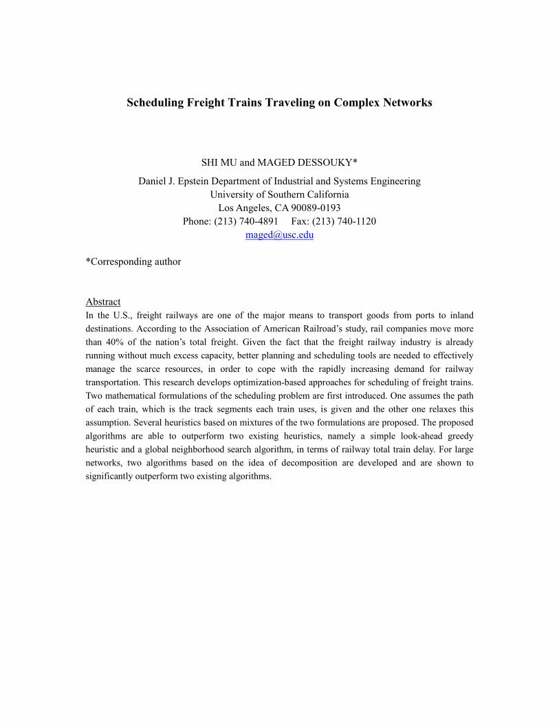
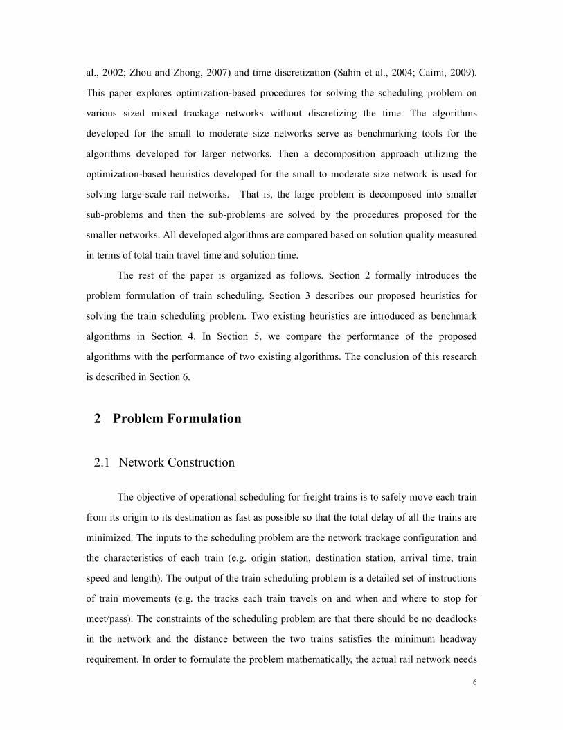
otherwise the track resource can not be fully utilized. A network construction of a portion of a

typical complex railway is shown in Figure 1. (Dessouky et al. 2006)

Figure 1 �etwork Construction

The length of the train can be longer than the length of a node. Thus a train can

occupy several nodes simultaneously. In reality, a train can travel at various speeds. The

acceleration and deceleration rates depend on a number of factors like locomotive power,

train weight and track slope. Lu et al. (2004) and Suteewong (2006) explicitly model the

acceleration and deceleration rates of the train. However, in order to make the mathematical

model plausible, we assume trains travel at their maximum speed. In all the following models,

no speed limits are imposed on the nodes. Trains pass each node at its maximum speed. Also

the train tracks are divided into nodes with length greater than the maximum length of all the

trains. This ensures a single train can occupy at most two nodes at a time, while maintaining

minimum headway clearance.

The schedule specifies the path each train takes and the arrival and departure times of

each train on every node of the specified path. A path is the sequence of nodes to be traversed

by the train, from its origin to its destination. Next we are going to introduce two

8

mathematical formulations of the scheduling problem. The first formulation assumes the path

for each train is given and the second formulation treats the path of each train as variables of

the model.

2.2 Fixed Path Formulation

The first model in the literature that we use for benchmarking purpose is the mixed

integer programming model introduced by Dessouky et al. (2006). Carey and Lockwood

(1995) develop a similar model which focuses on passenger railways. We refer the model

formulated by Dessouky et al. (2006) as FixedPath, since the exact path of each train needs to

be specified before solving the model. We now formally introduce the FixedPath model.

Notations:

Q : Set of all the trains to be scheduled

� : Set of all rail track nodes

qS : Length of train q, ,q Q∈ 1,2,...,q Q=

qP : Path train q takes. Starts with train q’s origin node, 0

qn , to train q’s

destination node, z

qn . All the nodes train q will be traversing are:

,1 ,2 ,{ , ,..., }

qq q q p

n n n , where 0

1, qq nn = and , q

z

qq Pn n=

1

,q gB : The minimal travel time between train q’s head entering into node ,q gn and

train q’s head leaving from node ,q gn to node , 1q gn +

2

, :q gB The minimal travel time between train q’s head entering into node ,q gn and

train q’s tail leaving node ,q gn

, :a

q gt The time train q’s head arrives at node ,q gn

, :d

q gt The time train q’s tail leaves from node ,q gn

µ : Minimal safety headway between two consecutive trains

:,, 21 kqqx Binary variable indicates which train gets to pass node k first. 1: train

9

1q passes node k before train 2q . 0: train 2q passes node k before train

1q .

M: An arbitrarily large number

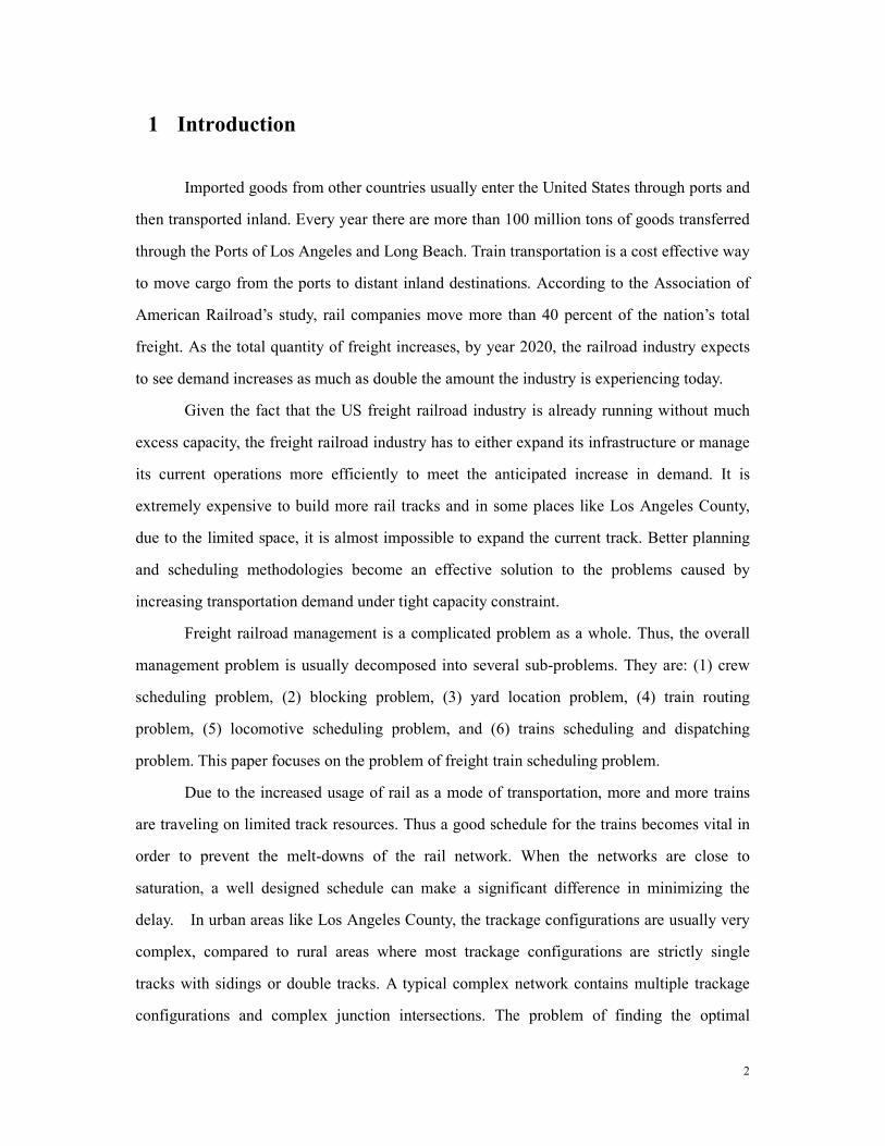
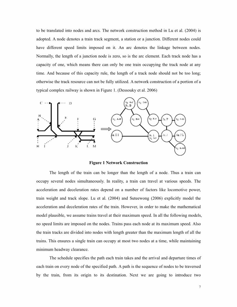
Figure 2 Relationship between variables

In Figure 2, we show the relationship between variables ,

a

q gt , , 1

a

q gt + , ,

d

q gt , 1

,q gB and

2

,q gB . Since the length of the train is taken into account, the variable , 1

a

q gt + is always smaller

then variable ,

d

q gt . The 0-1 mixed integer programming formulation of FixedPath is

described as follows:

,min (1)

. .

q

a

q Pq Q

t

s t

∈∑

1

, 1 , ,

2 1

, , 1 , ,

, for all and 1 1 (2)

, for all

a a

q g q g q g q

d a

q g q g q g q g

t t B q Q g P

t t B B q Q

+

+

− ≥ ∈ ≤ ≤ −

− ≥ − ∈

1 2 1 2

2

, , ,

, , , ,

and 1 1 (3)

, for all (4)

for all

q q q

q

d a

q P q P q P

a d

q q k q g q h

g P

t t B q Q

x M t t µ

≤ ≤ −

− ≥ ∈

+ ≥ +

{ }

1 2

1 2 2 1 1 2

1 2

1 2 , ,

, , , , 1 2 , ,

, , 1 2

, and node (5)

(1 ) for all , and node (6)

0,1 for all , and 1

q g q h

a d

q q k q h q g q g q h

q q k

q q Q k n n

x M t t q q Q k n n

x q q Q k �

µ

∈ = =

− + ≥ + ∈ = =

= ∈ ≤ ≤ (7)

The objective function (1) minimizes the sum of the arrival times of all trains at their

destinations which is equal to the total delay of all the trains. Constraint (2) ensures the

Node ,q gn Node , 1q gn +

1

,q gB

2

,q gB

,

a

q gt , 1

a

q gt + ,

d

q gt

10

minimum traveling time of the train on each track. The equal or greater sign makes it possible

for a train to wait for its next required resource to be cleared. Constraint (3) ensures the

minimum time a train needs to completely clear its previous occupied resource, after its head

enters the next node. The deadlock avoidance mechanism is realized by constraints (5) and

(6). These constraints together make sure that no more than one train can occupy the same

node simultaneously. If train 1q gets to pass node k before train 2q , the arrival time of

2q

at node k has to be equal to or greater than the departure time of 1q from node k plus the

safety headway of µ , and vice versa.

The FixedPath model can be used to solve the scheduling problem for any general

network, as long as the length of each node is not shorter than the maximum length of each

train. The formulation of FixedPath can be solved using a commercially available

optimization solver like CPLEX. The major drawback of the FixedPath algorithm is, as its

name suggests, the exact path of each train needs to be fixed and serves as the input to the

model. However, the sequence of nodes a train travels is an important factor that can affect

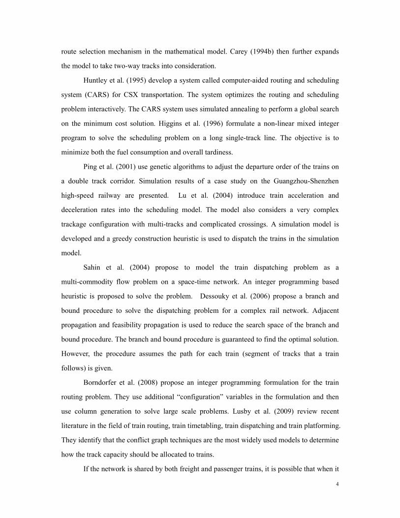
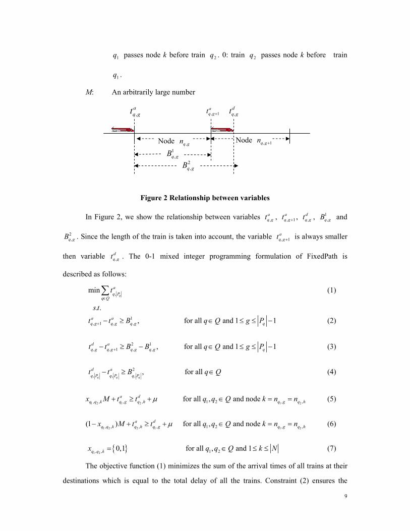
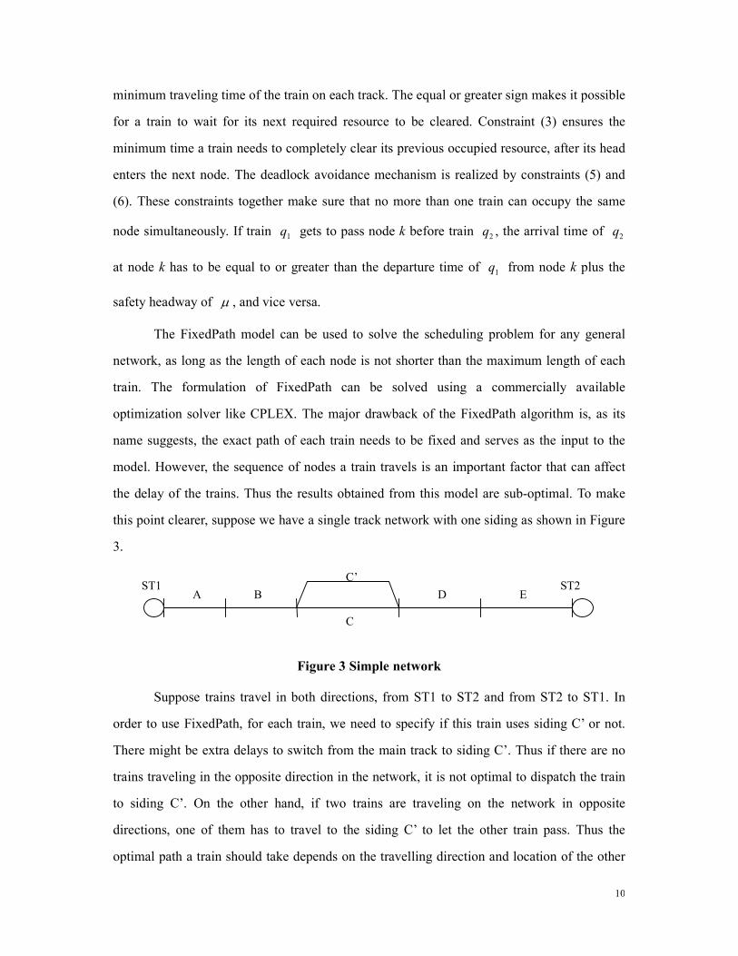
the delay of the trains. Thus the results obtained from this model are sub-optimal. To make

this point clearer, suppose we have a single track network with one siding as shown in Figure

3.

Figure 3 Simple network

Suppose trains travel in both directions, from ST1 to ST2 and from ST2 to ST1. In

order to use FixedPath, for each train, we need to specify if this train uses siding C’ or not.

There might be extra delays to switch from the main track to siding C’. Thus if there are no

trains traveling in the opposite direction in the network, it is not optimal to dispatch the train

to siding C’. On the other hand, if two trains are traveling on the network in opposite

directions, one of them has to travel to the siding C’ to let the other train pass. Thus the

optimal path a train should take depends on the travelling direction and location of the other

A

C

B D E

C’ ST1 ST2

11

trains. Fixing the path before solving the scheduling problem can lead to a solution far from

the global optimal solution. And if there are both slow and fast trains on the network, fixing

the path might prevent the fast train, if it follows a slower train, from overtaking the slower

train.

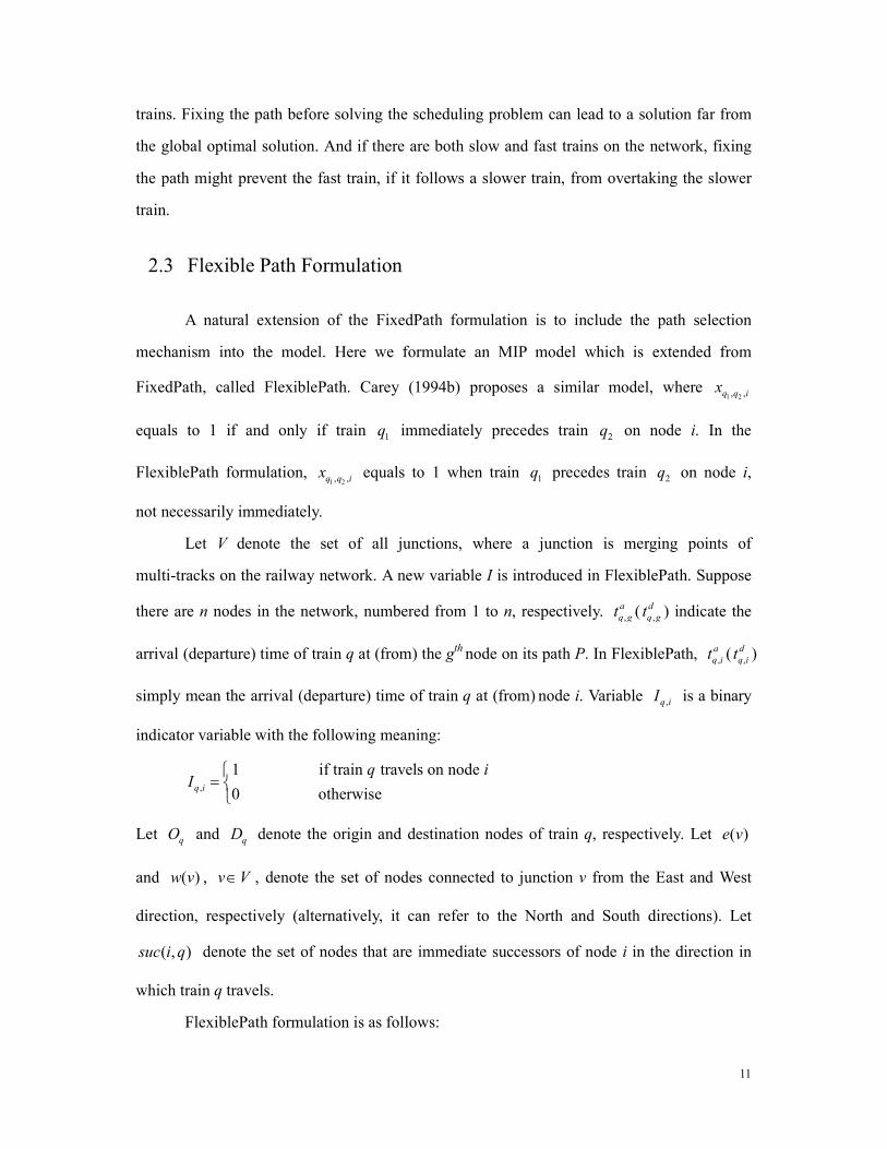
2.3 Flexible Path Formulation

A natural extension of the FixedPath formulation is to include the path selection

mechanism into the model. Here we formulate an MIP model which is extended from

FixedPath, called FlexiblePath. Carey (1994b) proposes a similar model, where 1 2, ,q q ix

equals to 1 if and only if train 1q immediately precedes train

2q on node i. In the

FlexiblePath formulation, 1 2, ,q q ix equals to 1 when train 1q precedes train 2q on node i,

not necessarily immediately.

Let V denote the set of all junctions, where a junction is merging points of

multi-tracks on the railway network. A new variable I is introduced in FlexiblePath. Suppose

there are n nodes in the network, numbered from 1 to n, respectively. ,

a

q gt ( ,

d

q gt ) indicate the

arrival (departure) time of train q at (from) the gth node on its path P. In FlexiblePath, ,

a

q it ( ,

d

q it )

simply mean the arrival (departure) time of train q at (from) node i. Variable ,q iI is a binary

indicator variable with the following meaning:

,

1 if train travels on node

0 otherwise q i

q iI

=

Let qO and qD denote the origin and destination nodes of train q, respectively. Let ( )e v

and ( )w v , v V∈ , denote the set of nodes connected to junction v from the East and West

direction, respectively (alternatively, it can refer to the North and South directions). Let

( , )suc i q denote the set of nodes that are immediate successors of node i in the direction in

which train q travels.

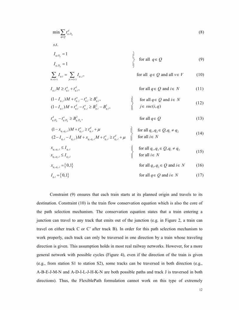
FlexiblePath formulation is as follows:

12

,min (8)

. .

q

d

q D

q Q

t

s t

∈∑

,

,

, ,

( )

1

for all (9)1

q

q

q O

q D

q i q j

i e v

I

q QI

I I∈

=

∈=

=∑( )

, for all and all (10)j w v

q Q v V∈

∈ ∈∑

, , ,

1

, , , ,

2 1

, , , , ,

, for all and (11)

(1 ) ,

(1 ) ,

a d

q i q i q i

a a

q j q j q i q i

d a

q i q i q j q i q i

I M t t q Q i �

I M t t B

I M t t B B

≥ + ∈ ∈

− + − ≥

− + − ≥ −

for all and (12)

( , )

q Q i �

j suc i q

∈ ∈

∈

1 2 2 1

1 2 1 2 1 2

2

, , ,

, , , ,

, , , , , ,

, for all (13)

(1 )

(2 )

q q q

d a

q D q D q D

a d

q q i q i q i

a d

q i q i q q i q i q i

t t B q Q

x M t t

I I M x M t t

µ

µ

− ≥ ∈

− + ≥ +

− − + + ≥ +

1 2 1

1 2 2

1 2 1 2

, , , 1 2 1 2

, , ,

for all , , (14)for all

for all , ,

for all

q q i q i

q q i q i

q q Q q q

i �

x I q q Q q q

x I i �

∈ ≠

∈

≤ ∈ ≠

≤ ∈

{ }

{ }

1 2, , 1 2

,

(15)

0,1 for all , and (16)

0,1

q q i

q i

x q q Q i �

I

= ∈ ∈

= for all and (17)q Q i �∈ ∈

Constraint (9) ensures that each train starts at its planned origin and travels to its

destination. Constraint (10) is the train flow conservation equation which is also the core of

the path selection mechanism. The conservation equation states that a train entering a

junction can travel to any track that emits out of the junction (e.g. in Figure 2, a train can

travel on either track C or C’ after track B). In order for this path selection mechanism to

work properly, each track can only be traversed in one direction by a train whose traveling

direction is given. This assumption holds in most real railway networks. However, for a more

general network with possible cycles (Figure 4), even if the direction of the train is given

(e.g., from station S1 to station S2), some tracks can be traversed in both direction (e.g.,

A-B-E-J-M-N and A-D-I-L-J-H-K-N are both possible paths and track J is traversed in both

directions). Thus, the FlexiblePath formulation cannot work on this type of extremely

13

complex network. However, the FixedPath formulation and the heuristics we propose which

are based on the FixedPath formulation can help generate a good schedule on these types of

complex networks.

Figure 4 A more general network

Constraint (11) states that if a train does not utilize track node i, then the arrival time

and departure time of that train on node i should be zero. Constraint (12) calculates the arrival

time and departure time on track nodes along the path that the train travels. Constraint (14) is

the deadlock avoidance constraint. In the formulation of FixedPath, variable 1 2, ,q q ix only

exists when both trains 1q and 2q have track node i on their paths. Here in FlexiblePath,

we have the variable 1 2, ,q q ix for any 1q and 2q pair on every track node. If

1 2, ,q q ix equals

to 1, this means 1q and 2q both travel on node i and 1q gets to pass node i before 2q . If

1 2, ,q q ix equals to 0, either one of the two situations happen: at least one of the two trains does

not travel on node i or both 1q and 2q travel on node i and 2q passes node i before 1q .

Constraint (15) forces 1 2, ,q q ix to be 0 when either or both trains do not travel on node i.

For the same scheduling problem, the formulation of FlexiblePath contains far more

binary variables than that for FixedPath. Additional binary variables ,q iI are introduced in

the FlexiblePath formulation. The number of 1 2, ,q q ix variables in the FlexiblePath

formulation is much larger then the number of 1 2, ,q q kx variables in the FixedPath formulation,

because these variables in the FlexiblePath formulation exist for every train pair on every

node and these variables in the FixedPath formulation only exist if train 1q and 2q are both

A B C

D

I

G

L

H

M

E

J

F

K

N

S1

S2

14

traveling on node k. Since we know the path for all the trains in the FixedPath formulation,

we only need to introduce a limited number of 1 2, ,q q kx variables. Similarly, for the

FlexiblePath formulation, we need variables of arrival and departure times of every train on

every node. But for the FixedPath formulation, we only need variables of arrival and

departure times of each train for nodes on its predetermined path. The solution computing

time of FlexiblePath would be far greater than the time required for FixedPath. However a

significant reduction of total delay might be achieved by incorporating the path selection

mechanism of FlexiblePath. We now show the performance of both formulations by a

computational experiment on an example network.

2.4 Experimental Results

In this sub-section, we compare the performances of the FixedPath and FlexiblePath

formulations. Though the majority of the numerical experiments are shown in Section 5, we

present some results to illustrate the tradeoff between solution quality and the solution CPU

time for both formulations. Finding a better tradeoff between solution quality and solution

time becomes the key motivation for our proposed algorithms.

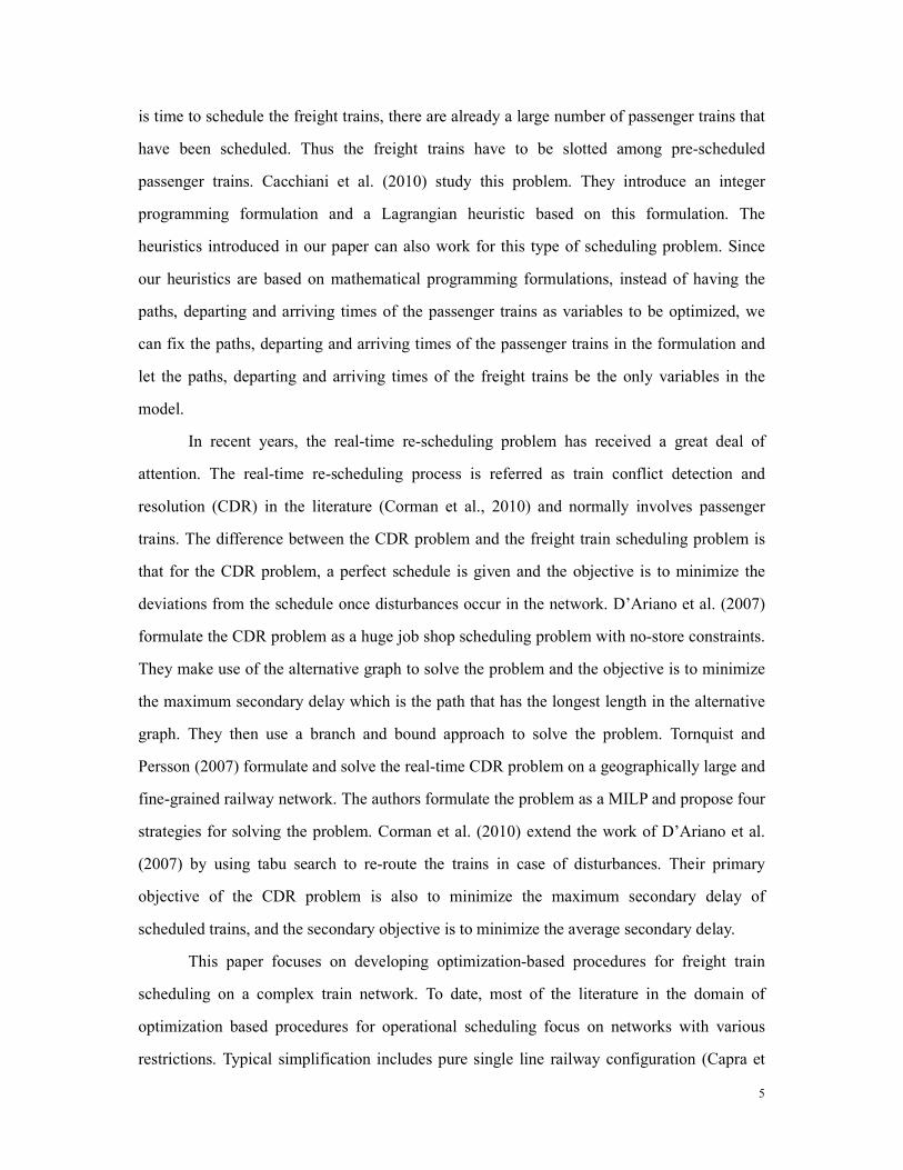
The experiment is based on a portion of the real network in Los Angeles County (see

Figure 5). The numbers in Figure 5 denote the lengths of the track components (in miles).

The trains traveling from west to east arrive at point A and are routed to point D. For the other

direction, the trains enter the network from point C and are routed to point B. From the

preliminary computational experiments, we found that for this network, the maximum

number of trains that FlexiblePath can solve optimally is four, given a solving time constraint

of one hour of CPU time. Both formulations are tested under four scenarios. In each scenario,

two trains travel in the eastbound direction and the other two trains travel in the westbound

direction. The details of the four scenarios are listed in Table 1.

15

Figure 5 Moderate Size network for numerical example

Table 1 Description of the scenarios (4 trains)

The parameters of the four scenarios ensure the computational experiments mimic the

real situation as close as possible. The ready times of each train is uniformly distributed.

Scenarios 1 and 2 have tighter schedules than scenarios 3 and 4. The uniform distribution U(0,

10) and U(0, 20) are chosen so that there is significant difference between scenarios 1,2 and

scenarios 3,4, and trains in all four scenarios are not too dense nor too sparse. In reality, the

maximum speed of a passenger train can be as high as 1.35 mile/minute, whereas the

maximum speed of a freight train can be as low as 0.7 mile/minute. The four possible speeds

(0.75, 1, 1.25 and 1.5) ensure trains travel at different speeds as they do in reality. The

average speed difference in scenarios 2 and 4 is larger than the difference in scenarios 1 and 3.

Also, in reality the trains have different lengths. Typical passenger and freight trains have

lengths of 0.189 and 1.136 mile. These stochastic elements lead to different meet and pass

situation between trains. Thus, the performances of FixedPath and FlexiblePath are fully

assessed. A penalty time (denoted by p) of 0.5 minute is added for each time a train switches

lines (e.g. a train switches to siding from the main line). This penalty time can be

implemented by modifying constraint (5) of FlexiblePath and constraint (2) of FixedPath: if

traveling from node i to node j involves switching of line, then 1

, , ,

a a

q j q i q it t B p− ≥ + .

4 trains Train ready time (minute) Train speed (miles/min) Train length (mile)

Scenario 1 Uniform(0,10) 0.75, 1, 1.25 and 1.5 (equally likely) 0.189 and 1.136 (equally likely)

Scenario 2 Uniform(0,10) 0.75 and 1.5 (equally likely) 0.189 and 1.136 (equally likely)

Scenario 3 Uniform(0,20) 0.75, 1, 1.25 and 1.5 (equally likely) 0.189 and 1.136 (equally likely)

Scenario 4 Uniform(0,20) 0.75 and 1.5 (equally likely) 0.189 and 1.136 (equally likely)

2.68

D

2.34

1.68 2.68

1.68 2.68

2.17

1.68

1.68

1.68 A

B

C

S P Q

SW1 SW2

16

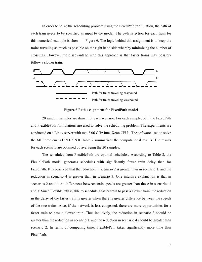
In order to solve the scheduling problem using the FixedPath formulation, the path of

each train needs to be specified as input to the model. The path selection for each train for

this numerical example is shown in Figure 6. The logic behind this assignment is to keep the

trains traveling as much as possible on the right hand side whereby minimizing the number of

crossings. However the disadvantage with this approach is that faster trains may possibly

follow a slower train.

Figure 6 Path assignment for FixedPath model

20 random samples are drawn for each scenario. For each sample, both the FixedPath

and FlexiblePath formulations are used to solve the scheduling problem. The experiments are

conducted on a Linux server with two 3.06 GHz Intel Xeon CPUs. The software used to solve

the MIP problem is CPLEX 9.0. Table 2 summarizes the computational results. The results

for each scenario are obtained by averaging the 20 samples.

The schedules from FlexiblePath are optimal schedules. According to Table 2, the

FlexiblePath model generates schedules with significantly fewer train delay than for

FixedPath. It is observed that the reduction in scenario 2 is greater than in scenario 1, and the

reduction in scenario 4 is greater than in scenario 3. One intuitive explanation is that in

scenarios 2 and 4, the differences between train speeds are greater than those in scenarios 1

and 3. Since FlexiblePath is able to schedule a faster train to pass a slower train, the reduction

in the delay of the faster train is greater when there is greater difference between the speeds

of the two trains. Also, if the network is less congested, there are more opportunities for a

faster train to pass a slower train. Thus intuitively, the reduction in scenario 3 should be

greater than the reduction in scenario 1, and the reduction in scenario 4 should be greater than

scenario 2. In terms of computing time, FlexiblePath takes significantly more time than

FixedPath.

A

B

C

D

Path for trains traveling eastbound

Path for trains traveling westbound

17

Table 2 FlexiblePath V.S. FixedPath

Total train delay

under FixedPath

(minute)

Total train delay under

FlexiblePath (minute)

FixedPath delay

/FlexiblePath delay

FixedPath

CPU time (sec)

FlexiblePath

CPU time (sec)

Scenario 1 12.00 7.53 1.594 0.02 256.68

Scenario 2 12.91 7.64 1.690 0.02 214.82

Scenario 3 10.50 6.48 1.620 0.02 351.94

Scenario 4 12.25 6.47 1.893 0.02 280.49

3 Proposed Algorithms

3.1 LtdFlePath Algorithm

Since the number of integer variables increase exponentially as the number of trains

increases. Using the FlexiblePath formulation, an optimal solution cannot be obtained within

one hour of CPU time when the number of trains increases to 6 (3 in each direction) for the

sample network. The FlexiblePath formulation tends to explore every possible path for each

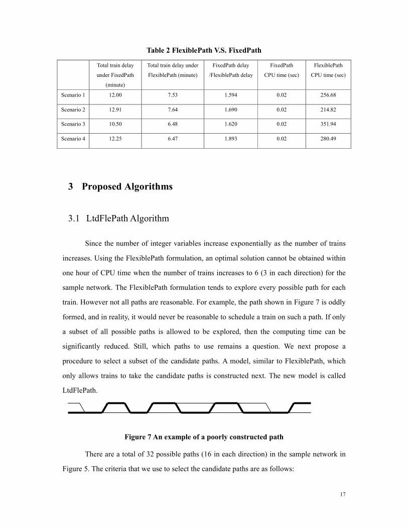
train. However not all paths are reasonable. For example, the path shown in Figure 7 is oddly

formed, and in reality, it would never be reasonable to schedule a train on such a path. If only

a subset of all possible paths is allowed to be explored, then the computing time can be

significantly reduced. Still, which paths to use remains a question. We next propose a

procedure to select a subset of the candidate paths. A model, similar to FlexiblePath, which

only allows trains to take the candidate paths is constructed next. The new model is called

LtdFlePath.

Figure 7 An example of a poorly constructed path

There are a total of 32 possible paths (16 in each direction) in the sample network in

Figure 5. The criteria that we use to select the candidate paths are as follows:

18

� The sidings are placed in the network for the purpose of meet and pass. Thus it is

important to leave the siding and the main line track beside the siding as options

for every train to take.

� Trains should have freedom to traverse along any track lines of the double tracks

or triple tracks without switching. This minimizes delay due to crossovers. In the

sample network, for the double tracks between points P and Q, trains at point P (Q)

could choose the upper or lower tracks and traverse all the way towards point Q (P)

without switching.

� If switching between the double or triple tracks are allowed, the first possible track

to switch along the train’s travel direction should be considered. By doing so,

trains traveling in the same direction but at different speeds, can make use of this

switch to complete the pass as early as possible. In the example, the switch

denoted by SW1 can be used by the trains traveling eastbound. Thus a faster train

can take over a slower train and both trains can continue traveling on the lower line

after SW1, leaving the upper line for the trains traveling westbound. Under the

same logic, trains traveling westbound should be allowed to make use of SW2.

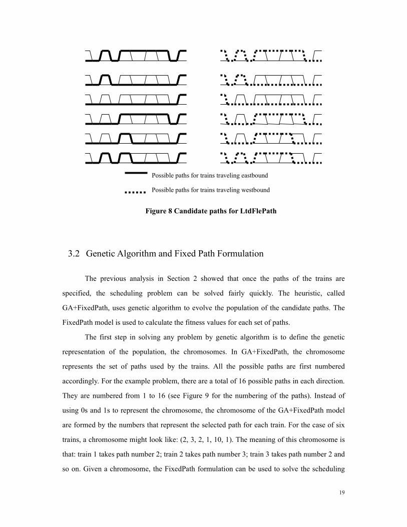
Preliminary experiments show that, for the example network, limiting the number of

paths to be under six makes it possible to solve the problem using the LtdFlePath model in a

reasonable amount of time. Following the three proposed criterions for selecting candidate

paths, for the example network, six paths (see Figure 8) for each direction are chosen to be

possible paths for model LtdFlePath. This is a reduction of the 16 possible paths that a train

can take in each direction.

LtdFlePath is very similar to FlexiblePath. The only difference in the formulation is in

constraint (2) in FlexiblePath. LtdFlePath modifies constraint (2) so that only the candidate

paths are allowed.

19

Figure 8 Candidate paths for LtdFlePath

3.2 Genetic Algorithm and Fixed Path Formulation

The previous analysis in Section 2 showed that once the paths of the trains are

specified, the scheduling problem can be solved fairly quickly. The heuristic, called

GA+FixedPath, uses genetic algorithm to evolve the population of the candidate paths. The

FixedPath model is used to calculate the fitness values for each set of paths.

The first step in solving any problem by genetic algorithm is to define the genetic

representation of the population, the chromosomes. In GA+FixedPath, the chromosome

represents the set of paths used by the trains. All the possible paths are first numbered

accordingly. For the example problem, there are a total of 16 possible paths in each direction.

They are numbered from 1 to 16 (see Figure 9 for the numbering of the paths). Instead of

using 0s and 1s to represent the chromosome, the chromosome of the GA+FixedPath model

are formed by the numbers that represent the selected path for each train. For the case of six

trains, a chromosome might look like: (2, 3, 2, 1, 10, 1). The meaning of this chromosome is

that: train 1 takes path number 2; train 2 takes path number 3; train 3 takes path number 2 and

so on. Given a chromosome, the FixedPath formulation can be used to solve the scheduling

Possible paths for trains traveling eastbound

Possible paths for trains traveling westbound

20

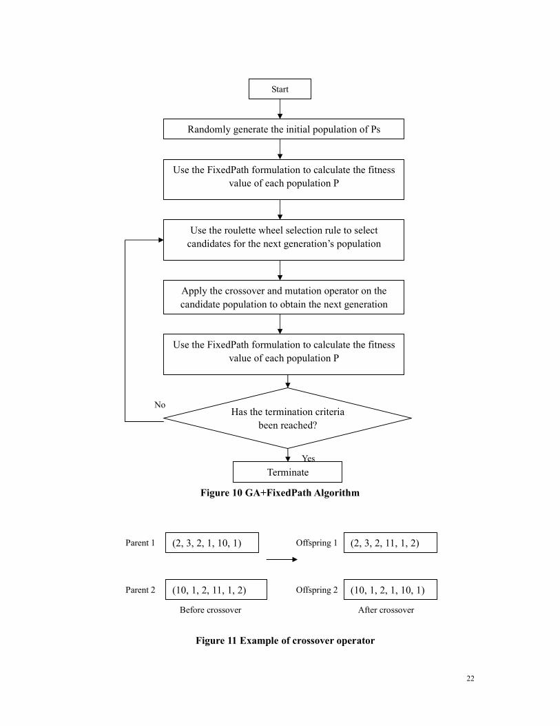
problem. The returned delay is treated as the fitness value of this chromosome. Let P denote a

single chromosome. The GA+FixedPath algorithm is described in the flowchart in Figure 10.

The initial population is randomly generated. However the paths do not have equal

probability of being selected by a train. The probabilities are adjusted so that a common and

reasonable path has a higher probability than an odd path (e.g., path 2 in the example network

should be selected with a higher probability than path 8). Sample probabilities of each path

being selected in the initial population are shown in Figure 9 for the sample network (the

notation “w/p” stands for “with probability”). The basic idea behind the selection of this

particular set of probabilities are: (1) paths 1, 2, 3 and 10 are common reasonable paths for

both directions according to the previous selection criteria and the total probabilities of these

four paths is set to 0.5, and (2) paths 11 and 12 are also reasonable paths according to the

selection criteria and they have fewer switches as compared to paths 4 and 5 and thus these

two paths are chosen with slightly higher probability than the rest of the paths. These

probabilities are experimentally shown to be a good choice. Once the initial generation is

created, the FixedPath formulation is used to obtain the fitness value of each population in the

initial generation. After associating each population with a fitness value, the roulette wheel

selection algorithm is used to select the parent chromosomes which will be used to produce

the next generation. The roulette wheel selection algorithm assures the higher the fitness a

chromosome has, the higher the chance it is selected.

21

1:

2:

3:

4:

5:

6:

7:

8:

9:

10:

11:

12:

13:

14:

15:

16:

w/p:0.125

w/p:0.125

w/p:0.125

w/p:0.125

w/p:0.035 w/p:0.075

w/p:0.035

w/p:0.035

w/p:0.035

w/p:0.035

w/p:0.035

w/p:0.075

w/p:0.035

w/p:0.035

w/p:0.035

w/p:0.035

Figure 9 �umbering of the paths and their probabilities of being selected in the initial

population (for both eastbound and westbound trains)

The crossover operation is then applied to the parent chromosomes. Since the first

half of the chromosome denotes the trains traveling in one direction and the second half of

the chromosome denotes the trains traveling in the opposite direction, it is reasonable to use

the single cut point crossover policy. The single cut point is made at the middle of the

chromosome. Figure 11 shows an example of the crossover operation. The crossover

operation is only carried out with a certain probability which is decided by the crossover

ratio.

22

Figure 10 GA+FixedPath Algorithm

Figure 11 Example of crossover operator

Randomly generate the initial population of Ps

Start

Use the FixedPath formulation to calculate the fitness

value of each population P

Use the roulette wheel selection rule to select

candidates for the next generation’s population

Apply the crossover and mutation operator on the

candidate population to obtain the next generation

Use the FixedPath formulation to calculate the fitness

value of each population P

Has the termination criteria

been reached?

Terminate

No

Yes

(2, 3, 2, 1, 10, 1)

(10, 1, 2, 11, 1, 2)

Parent 1

Parent 2

Offspring 1

Offspring 2

(2, 3, 2, 11, 1, 2)

(10, 1, 2, 1, 10, 1)

Before crossover After crossover

23

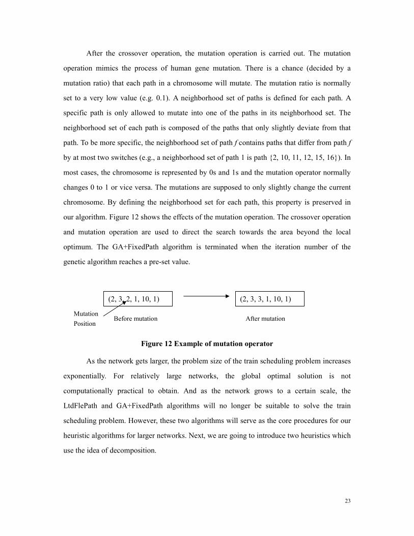
After the crossover operation, the mutation operation is carried out. The mutation

operation mimics the process of human gene mutation. There is a chance (decided by a

mutation ratio) that each path in a chromosome will mutate. The mutation ratio is normally

set to a very low value (e.g. 0.1). A neighborhood set of paths is defined for each path. A

specific path is only allowed to mutate into one of the paths in its neighborhood set. The

neighborhood set of each path is composed of the paths that only slightly deviate from that

path. To be more specific, the neighborhood set of path f contains paths that differ from path f

by at most two switches (e.g., a neighborhood set of path 1 is path {2, 10, 11, 12, 15, 16}). In

most cases, the chromosome is represented by 0s and 1s and the mutation operator normally

changes 0 to 1 or vice versa. The mutations are supposed to only slightly change the current

chromosome. By defining the neighborhood set for each path, this property is preserved in

our algorithm. Figure 12 shows the effects of the mutation operation. The crossover operation

and mutation operation are used to direct the search towards the area beyond the local

optimum. The GA+FixedPath algorithm is terminated when the iteration number of the

genetic algorithm reaches a pre-set value.

Figure 12 Example of mutation operator

As the network gets larger, the problem size of the train scheduling problem increases

exponentially. For relatively large networks, the global optimal solution is not

computationally practical to obtain. And as the network grows to a certain scale, the

LtdFlePath and GA+FixedPath algorithms will no longer be suitable to solve the train

scheduling problem. However, these two algorithms will serve as the core procedures for our

heuristic algorithms for larger networks. Next, we are going to introduce two heuristics which

use the idea of decomposition.

(2, 3, 2, 1, 10, 1) (2, 3, 3, 1, 10, 1)

Before mutation After mutation Mutation

Position

24

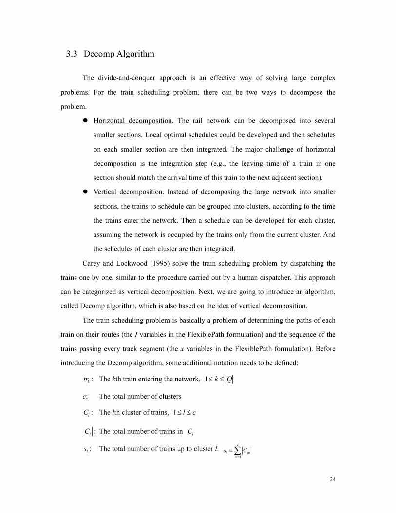
3.3 Decomp Algorithm

The divide-and-conquer approach is an effective way of solving large complex

problems. For the train scheduling problem, there can be two ways to decompose the

problem.

� Horizontal decomposition. The rail network can be decomposed into several

smaller sections. Local optimal schedules could be developed and then schedules

on each smaller section are then integrated. The major challenge of horizontal

decomposition is the integration step (e.g., the leaving time of a train in one

section should match the arrival time of this train to the next adjacent section).

� Vertical decomposition. Instead of decomposing the large network into smaller

sections, the trains to schedule can be grouped into clusters, according to the time

the trains enter the network. Then a schedule can be developed for each cluster,

assuming the network is occupied by the trains only from the current cluster. And

the schedules of each cluster are then integrated.

Carey and Lockwood (1995) solve the train scheduling problem by dispatching the

trains one by one, similar to the procedure carried out by a human dispatcher. This approach

can be categorized as vertical decomposition. Next, we are going to introduce an algorithm,

called Decomp algorithm, which is also based on the idea of vertical decomposition.

The train scheduling problem is basically a problem of determining the paths of each

train on their routes (the I variables in the FlexiblePath formulation) and the sequence of the

trains passing every track segment (the x variables in the FlexiblePath formulation). Before

introducing the Decomp algorithm, some additional notation needs to be defined:

ktr : The kth train entering the network, 1 k Q≤ ≤

c: The total number of clusters

lC : The lth cluster of trains, 1 l c≤ ≤

lC : The total number of trains in lC

ls : The total number of trains up to cluster l. 1

l

l m

m

s C=

=∑

25

Decomp Algorithm

Step 1: Decompose all the trains into clusters according to the entering time of the trains. lC

will contain trains 1 1lstr− +

, 1 2lstr− +

up to lstr .

Step 2:

Let l = 1;

While (l < c+1) {

Solve the scheduling problem (referred as sub-problem l) that only involves trains in

clusters 1 2, ,..., lC C C ;

Save and fix the values of variables ,q iI and1 2, ,q q ix , where 1 2 1 2, , ( , ,..., )lq q q C C C∈∪

and i �∈ , for the next iteration;

l= l +1;

}

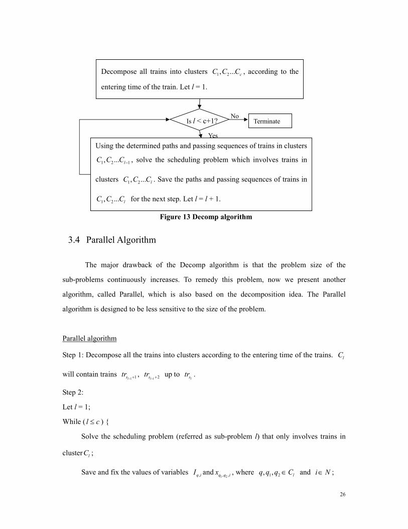
The description of the Decomp algorithm (also illustrated in Figure 13) only serves as

a general approach, there are two details that need to be decided.

1. The cluster size. The trade off between a large and small cluster size is very clear.

The larger the cluster size is, the better the solution quality is. But the larger the

cluster size is, the longer it takes to solve the sub-problem.

2. Algorithm used to solve sub-problems. Since the sub-problem itself is a smaller

version of the train scheduling problem, there are many options in solving the

problem. As the cluster size varies, the most suitable algorithm will change.

After solving sub-problem l, the path of each train in clusters 1 2, ,..., lC C C will be

fixed, so will the sequence for those trains passing each track node. Solving sub-problem l

involves determining the paths for the trains in cluster lC , the sequence of the trains in lC

passing every node, and the precedence relationship between trains in lC and trains in

1 2 1, ,..., lC C C − . Thus if every cluster has the same size, the problem size of the sub-problems

continuously increases (e.g., it takes more time to solve sub-problem l+1 than sub-problem l).

26

Figure 13 Decomp algorithm

3.4 Parallel Algorithm

The major drawback of the Decomp algorithm is that the problem size of the

sub-problems continuously increases. To remedy this problem, now we present another

algorithm, called Parallel, which is also based on the decomposition idea. The Parallel

algorithm is designed to be less sensitive to the size of the problem.

Parallel algorithm

Step 1: Decompose all the trains into clusters according to the entering time of the trains. lC

will contain trains 1 1lstr− +

, 1 2lstr− +

up to lstr .

Step 2:

Let l = 1;

While ( l c≤ ) {

Solve the scheduling problem (referred as sub-problem l) that only involves trains in

cluster lC ;

Save and fix the values of variables ,q iI and1 2, ,q q ix , where 1 2, , lq q q C∈ and i �∈ ;

Decompose all trains into clusters 1 2, ... cC C C , according to the

entering time of the train. Let l = 1.

Is l < c+1?

Using the determined paths and passing sequences of trains in clusters

1 2 1, ... lC C C − , solve the scheduling problem which involves trains in

clusters 1 2, ... lC C C . Save the paths and passing sequences of trains in

1 2, ... lC C C for the next step. Let l = l + 1.

Terminate No

Yes

27

l= l +1;

}

Step 3:

Use FixedPath formulation to solve the problem with all Q trains. The paths of each train are

fixed as in the solution of Step 2. Some of the x variables are also fixed as follows:

1. For trains q1 and q2 belonging in the same cluster, 1 2, ,q q ix is fixed as in the

solution in Step 2, i �∈

2. If 1 2, , 1q i q iI I= = , set

1 2, , 1q q ix = and 2 1, , 0q q ix = , where 1 lq C∈ and 2 sq C∈ ,

2s l≥ + , for 1,..., 2l c= − and 3,...,s c= .

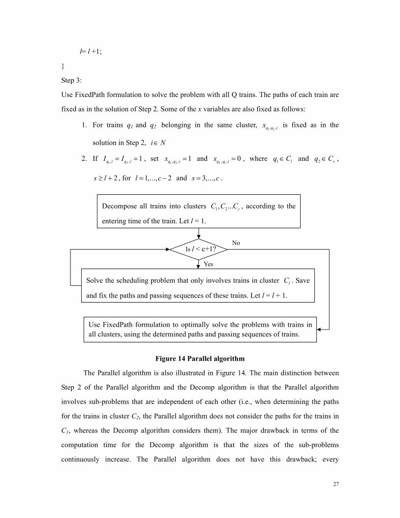
Figure 14 Parallel algorithm

The Parallel algorithm is also illustrated in Figure 14. The main distinction between

Step 2 of the Parallel algorithm and the Decomp algorithm is that the Parallel algorithm

involves sub-problems that are independent of each other (i.e., when determining the paths

for the trains in cluster C2, the Parallel algorithm does not consider the paths for the trains in

C1, whereas the Decomp algorithm considers them). The major drawback in terms of the

computation time for the Decomp algorithm is that the sizes of the sub-problems

continuously increase. The Parallel algorithm does not have this drawback; every

Decompose all trains into clusters 1 2, ... cC C C , according to the

entering time of the train. Let l = 1.

Is l < c+1?

Solve the scheduling problem that only involves trains in cluster lC . Save

and fix the paths and passing sequences of these trains. Let l = l + 1.

No

Yes

Use FixedPath formulation to optimally solve the problems with trains in

all clusters, using the determined paths and passing sequences of trains.

28

sub-problem is of the same size, if the cluster sizes are the same.

The algorithm is called Parallel, because in Step 2, a total number of c sub-problems

are solved independently, thus all the sub-problems can be solved in parallel. Nowadays,

most CPUs in personal computers have multiple processing cores. By solving the problem in

parallel, the computation time of Step 2 can be reduced by a factor of the number of CPU

cores.

Step 2 determines the paths of each train. Step 3 involves solving a scheduling

problem where the path of each train is given. However, given a relatively large network and

large number of trains, the FixedPath formulation can not solve Step 3 efficiently without

pre-fixing some of the x variables. The precedence rules for trains in the same cluster are

pre-fixed as the solution in Step 2. Also, to further reduce the solution space, the trains in

cluster l have precedence on every track node over all the trains in clusters l+2, l+3, …, c. So,

in Step 3, the FixedPath formulation is used to only determine the precedence rule between

trains in adjacent clusters.

In expectation, the Parallel algorithm runs faster than the Decomp algorithm, but

generates a schedule with higher delays.

4 Benchmark algorithms

In order to have a better idea of the performance of the proposed algorithms, we are

going to introduce two existing heuristics, one based on a simple insertion procedure while

the other based on a genetic algorithm approach, that we later use as benchmark algorithms

for freight train scheduling. These two particular procedures are chosen because they have

exactly the same objective as our problem and are intended for the same operational

conditions as our model (e.g. mixed trackage, freight train and long train lengths). Other train

scheduling algorithms that mainly focus on passenger trains either have a different objective

function or a different representation of the railway network (i.e. much shorter node length

because passenger trains are much shorter than freight trains). Furthermore, in the literature

the insertion and meta-heuristics approaches are common methods to solve moderate to large

29

scale train scheduling problems (Ping et al., 2001; Corman et al., 2010).

4.1 Pure Genetic Algorithm

Suteewong (2006) introduces a genetic algorithm to solve the train scheduling

problem (referred as PureGA algorithm). While the GA+FixedPath uses genetic algorithm to

evolve the paths of trains, the PureGA algorithm not only evolves the paths of each train but

also the precedence rules among the trains.

In PureGA algorithm, there are two types of chromosomes. One represents the 1 2, ,q q ix

variable and the other represents the,q iI variable.

1 2, ,q q ix controls the order of trains passing

through a certain track node. ,q iI equals 1 if train q passes on track i and 0 otherwise. The

chromosome of 1 2, ,q q ix is a three-dimensional matrix whose size is n n m× × , where n is the

total number of trains and m is the total number track nodes. ,q iI has a representation that is

a two-dimensional matrix whose dimension is n m× . The procedure of the PureGA

algorithm is as below:

1. Randomly generate an initial population for the 1 2, ,q q ix and

,q iI .

2. Calculate the objective function for each population.

3. Use the roulette wheel selection rule to select the parent chromosomes and then

use the crossover and mutation operators.

4. Obtain a new population for the 1 2, ,q q ix and ,q iI binary variables. Replace the

previous 1 2, ,q q ix and ,q iI with the new ones. Evaluate the new objective function.

5. Check the termination criteria. If it is met, terminate with the solution. Otherwise,

repeat step (3) through (5).

The x and I variables are correlated. As we stated in FlexiblePath, 1 2, ,q q ix is only

meaningful if 1 ,q iI and

2 ,q iI are both 1 (e.g. both trains q1 and q2 pass node i). This

correlation complicates the process of evolution of the chromosomes. Before the fitness value

of each population is assessed, a Repairing Algorithm needs to be applied to assure the

30

consistency between X and I variables. The Travel Time for �ode Algorithm (TTN) is

developed to determine the travel time for each individual node of a particular train. Another

algorithm called Deadlock Prevention Algorithm, which has TTN embedded in it as a

subroutine, is also developed. Given the new population of the x and I variables, the

Repairing Algorithm is first applied, and then the Deadlock Prevention Algorithm is applied

to return a deadlock-free schedule based on the x and I variables. The PureGA algorithm, not

like the GA+FixedPath algorithm, is not based on a mixed integer programming model. As

we will later see, in general, the PureGA algorithm runs faster than GA+FixedPath. But in

terms of solution quality, the GA+FixedPath outperforms the PureGA algorithm.

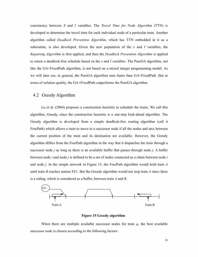
4.2 Greedy Algorithm

Lu et al. (2004) proposes a construction heuristic to schedule the trains. We call this

algorithm, Greedy, since the construction heuristic is a one-step look-ahead algorithm. The

Greedy algorithm is developed from a simple deadlock-free routing algorithm (call it

FreePath) which allows a train to move to a successor node if all the nodes and arcs between

the current position of the train and its destination are available. However, the Greedy

algorithm differs from the FreePath algorithm in the way that it dispatches the train through a

successor node j as long as there is an available buffer that passes through node j. A buffer

between node i and node j is defined to be a set of nodes connected as a chain between node i

and node j. In the simple network in Figure 15, the FreePath algorithm would hold train A

until train B reaches station ST1. But the Greedy algorithm would not stop train A since there

is a siding, which is considered as a buffer, between train A and B.

Figure 15 Greedy algorithm

When there are multiple available successor nodes for train q, the best available

successor node is chosen according to the following factors:

ST1

Train A Train B

31

1. The maximum priority difference between the current train and the immediate

successor train running in the same direction if one exists.

2. The maximal number of trains running in the same direction along the path from

the successor node to the train’s destination node.

3. The minimum travel time for the current train from the successor node to the

current train’s destination node assuming there is no downstream conflicting

traffic ahead of the current train.

The computing time of the Greedy algorithm is negligible even for relatively large

scale problems. It is the fastest among all the algorithms introduced. And it is not surprising

to see that it produces a schedule with the largest train delays.

5 Experimental results

In this section, we compare the performance of the proposed algorithms and

benchmark algorithms in three sample networks. The purpose of the numerical experiments is

to illustrate the tradeoff between the solution quality and solution CPU time for each

algorithm.

5.1 Small network

In Section 2, we compare the FixedPath formulation and FlexiblePath formulation for

the scenarios of 4 trains in the sample network. Next we present the results of the LtdFlePath,

GA+FixedPath, PureGA and Greedy algorithm for the same scenarios as in Section 2.

Though this sample network is relatively small, computational results on this network

provides us valuable insights on how far the schedules generated by our heuristic algorithms

are from the optimal schedule (e.g. generated by FlexiblePath model). Also, these

comparisons serve to show which heuristic (LtdFlePath and GA+FixedPath) should be used

to solve the sub-problems of the Decomp and Parallel algorithm. The Decomp and Parallel

algorithms are designed to work with large number of trains thus are not included in this

32

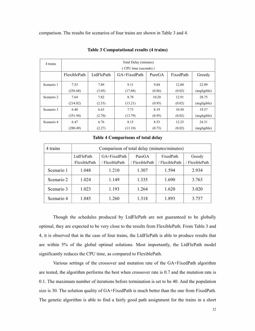
comparison. The results for scenarios of four trains are shown in Table 3 and 4.

Table 3 Computational results (4 trains)

Table 4 Comparisons of total delay

4 trains Comparison of total delay (minutes/minutes)

LtdFlePath

/FlexiblePath

GA+FixedPath

/ FlexiblePath

PureGA

/ FlexiblePath

FixedPath

/ FlexiblePath

Greedy

/ FlexiblePath

Scenario 1 1.048 1.210 1.307 1.594 2.934

Scenario 2 1.024 1.149 1.335 1.690 3.763

Scenario 3 1.023 1.193 1.264 1.620 3.020

Scenario 4 1.045 1.260 1.318 1.893 3.757

Though the schedules produced by LtdFlePath are not guaranteed to be globally

optimal, they are expected to be very close to the results from FlexiblePath. From Table 3 and

4, it is observed that in the case of four trains, the LtdFlePath is able to produce results that

are within 5% of the global optimal solutions. Most importantly, the LtdFlePath model

significantly reduces the CPU time, as compared to FlexiblePath.

Various settings of the crossover and mutation rate of the GA+FixedPath algorithm

are tested, the algorithm performs the best when crossover rate is 0.7 and the mutation rate is

0.1. The maximum number of iterations before termination is set to be 40. And the population

size is 30. The solution quality of GA+FixedPath is much better than the one from FixedPath.

The genetic algorithm is able to find a fairly good path assignment for the trains in a short

4 trains Total Delay (minutes)

( CPU time (seconds) )

FlexiblePath LtdFlePath GA+FixedPath PureGA FixedPath Greedy

Scenario 1 7.53

(256.68)

7.89

(3.05)

9.11

(17.08)

9.84

(0.86)

12.00

(0.02)

22.09

(negligible)

Scenario 2 7.64

(214.82)

7.82

(2.53)

8.78

(13.21)

10.20

(0.95)

12.91

(0.02)

28.75

(negligible)

Scenario 3 6.48

(351.94)

6.63

(2.70)

7.73

(13.79)

8.19

(0.95)

10.50

(0.02)

19.57

(negligible)

Scenario 4 6.47

(280.49)

6.76

(2.27)

8.15

(13.10)

8.53

(0.73)

12.25

(0.02)

24.31

(negligible)

33

time. The GA+FixedPath would be able to solve the scheduling problem when the size of the

problem further increases. The CPU solution time of GA+FixedPath algorithm is less

sensitive to the size of the problem compared to the LtdFlePath algorithm. As the number of

trains increases, GA+FixedPath algorithm would become more advantageous in terms of

solution time.

For the PureGA algorithm, the crossover and mutation rates are 0.6 and 0.1,

respectively. The population size is set to be 50 and the maximum iteration number is set to

be 100. From the results, we can see that the PureGA algorithm is outperformed by the

GA+FixedPath algorithm in terms of solution quality. This is because that given a specific

path assignment, the GA+FixedPath returns the optimal schedule for this path assignment.

The Greedy algorithm performs the worst in terms of solution quality, but it is the

computationally fastest algorithm. Even when the number of trains is small, there is a

significant gap in terms of solution quality between the Greedy Algorithm and the optimal

algorithms.

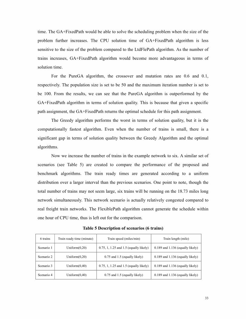
Now we increase the number of trains in the example network to six. A similar set of

scenarios (see Table 5) are created to compare the performance of the proposed and

benchmark algorithms. The train ready times are generated according to a uniform

distribution over a larger interval than the previous scenarios. One point to note, though the

total number of trains may not seem large, six trains will be running on the 18.73 miles long

network simultaneously. This network scenario is actually relatively congested compared to

real freight train networks. The FlexiblePath algorithm cannot generate the schedule within

one hour of CPU time, thus is left out for the comparison.

Table 5 Description of scenarios (6 trains)

6 trains Train ready time (minute) Train speed (miles/min) Train length (mile)

Scenario 1 Uniform(0,20) 0.75, 1, 1.25 and 1.5 (equally likely) 0.189 and 1.136 (equally likely)

Scenario 2 Uniform(0,20) 0.75 and 1.5 (equally likely) 0.189 and 1.136 (equally likely)

Scenario 3 Uniform(0,40) 0.75, 1, 1.25 and 1.5 (equally likely) 0.189 and 1.136 (equally likely)

Scenario 4 Uniform(0,40) 0.75 and 1.5 (equally likely) 0.189 and 1.136 (equally likely)

34

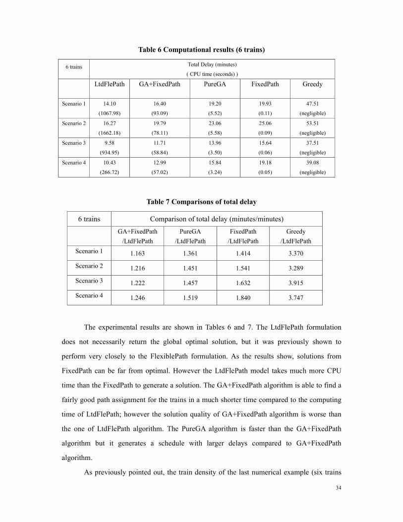
Table 6 Computational results (6 trains)

6 trains Total Delay (minutes)

( CPU time (seconds) )

LtdFlePath GA+FixedPath PureGA FixedPath

Greedy

Scenario 1 14.10

(1067.98)

16.40

(93.09)

19.20

(5.52)

19.93

(0.11)

47.51

(negligible)

Scenario 2 16.27

(1662.18)

19.79

(78.11)

23.06

(5.58)

25.06

(0.09)

53.51

(negligible)

Scenario 3 9.58

(934.95)

11.71

(58.84)

13.96

(3.50)

15.64

(0.06)

37.51

(negligible)

Scenario 4 10.43

(266.72)

12.99

(57.02)

15.84

(3.24)

19.18

(0.05)

39.08

(negligible)

Table 7 Comparisons of total delay

6 trains Comparison of total delay (minutes/minutes)

GA+FixedPath

/LtdFlePath

PureGA

/LtdFlePath

FixedPath

/LtdFlePath

Greedy

/LtdFlePath

Scenario 1 1.163 1.361 1.414 3.370

Scenario 2 1.216 1.451 1.541 3.289

Scenario 3 1.222 1.457 1.632 3.915

Scenario 4 1.246 1.519 1.840 3.747

The experimental results are shown in Tables 6 and 7. The LtdFlePath formulation

does not necessarily return the global optimal solution, but it was previously shown to

perform very closely to the FlexiblePath formulation. As the results show, solutions from

FixedPath can be far from optimal. However the LtdFlePath model takes much more CPU

time than the FixedPath to generate a solution. The GA+FixedPath algorithm is able to find a

fairly good path assignment for the trains in a much shorter time compared to the computing

time of LtdFlePath; however the solution quality of GA+FixedPath algorithm is worse than

the one of LtdFlePath algorithm. The PureGA algorithm is faster than the GA+FixedPath

algorithm but it generates a schedule with larger delays compared to GA+FixedPath

algorithm.

As previously pointed out, the train density of the last numerical example (six trains

35

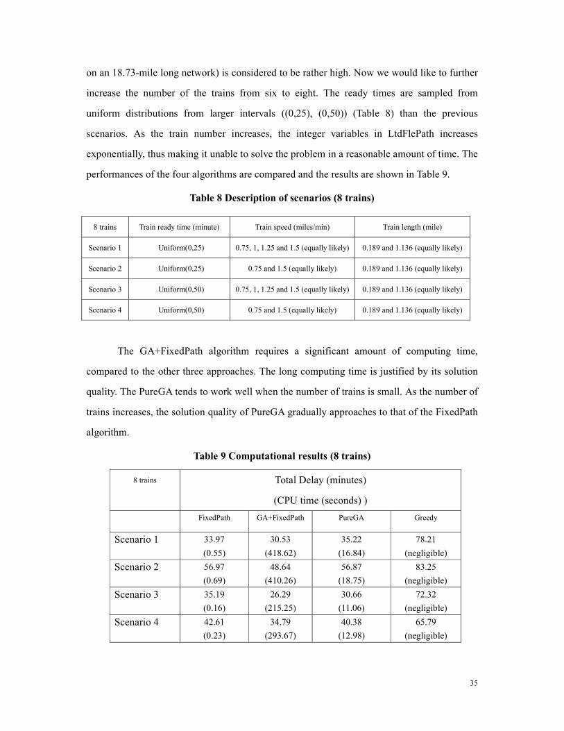
on an 18.73-mile long network) is considered to be rather high. Now we would like to further

increase the number of the trains from six to eight. The ready times are sampled from

uniform distributions from larger intervals ((0,25), (0,50)) (Table 8) than the previous

scenarios. As the train number increases, the integer variables in LtdFlePath increases

exponentially, thus making it unable to solve the problem in a reasonable amount of time. The

performances of the four algorithms are compared and the results are shown in Table 9.

Table 8 Description of scenarios (8 trains)

The GA+FixedPath algorithm requires a significant amount of computing time,

compared to the other three approaches. The long computing time is justified by its solution

quality. The PureGA tends to work well when the number of trains is small. As the number of

trains increases, the solution quality of PureGA gradually approaches to that of the FixedPath

algorithm.

Table 9 Computational results (8 trains)

8 trains Total Delay (minutes)

(CPU time (seconds) )

FixedPath GA+FixedPath PureGA Greedy

Scenario 1 33.97

(0.55)

30.53

(418.62)

35.22

(16.84)

78.21

(negligible)

Scenario 2 56.97

(0.69)

48.64

(410.26)

56.87

(18.75)

83.25

(negligible)

Scenario 3 35.19

(0.16)

26.29

(215.25)

30.66

(11.06)

72.32

(negligible)

Scenario 4 42.61

(0.23)

34.79

(293.67)

40.38

(12.98)

65.79

(negligible)

8 trains Train ready time (minute) Train speed (miles/min) Train length (mile)

Scenario 1 Uniform(0,25) 0.75, 1, 1.25 and 1.5 (equally likely) 0.189 and 1.136 (equally likely)

Scenario 2 Uniform(0,25) 0.75 and 1.5 (equally likely) 0.189 and 1.136 (equally likely)

Scenario 3 Uniform(0,50) 0.75, 1, 1.25 and 1.5 (equally likely) 0.189 and 1.136 (equally likely)

Scenario 4 Uniform(0,50) 0.75 and 1.5 (equally likely) 0.189 and 1.136 (equally likely)

36

5.2 Medium network

Now we would like to introduce a medium size network which is a portion of the

network of the area of downtown Los Angeles. This sample network is 33.86 miles long and

is a mixture of double-track and triple-track segments. The trackage configuration of this

sample network is shown in Appendix A. There are six stations in this network. Trains

travelling eastbound depart from station A and travel to either station C (e.g. a short route) or

station E (e.g. a long route). Trains travelling westbound depart from station F and travel to

either station D (e.g. a short route) or station B (e.g. a long route). The time interval between

two consecutive trains in the same direction is assumed to be uniformly distributed between 8

and 10 minutes. The train speed is equally likely to be 0.75, 1, 1.25 and 1.5 miles/minute and

the length of each train is equally likely to be 0.189 and 1.136 miles. Each train is going to

take the long route with probability 0.7 and the short route with probability 0.3.

For this network the LtdFlePath and GA+FixedPath algorithms themselves are

unable to generate a schedule within a reasonable amount of time. We focus on demonstrating

the performance of the Decomp and Parallel algorithms in this section.

For Decomp and Parallel algorithms, we have to determine the algorithm to solve the

sub-problems. If the LtdFlePath formulation is used to solve the sub-problems of the Decomp

and Parallel algorithms, the cluster size of 6 is found to be reasonable. If the GA+FixedPath

algorithm (population size: 20; crossover rate: 0.7; mutation rate: 0.1; maximum number of

iterations: 10) is used to solve the sub-problems, the cluster size is chosen to be fixed at 10

and 14 for the Decomp and Parallel algorithms, respectively. The cluster size of 14 for the

Parallel algorithm is bigger than the one used in the Decomp algorithm. The reason being that

the size of the sub-problem is constant for the Parallel algorithm, using a bigger cluster will

not result in intractable sub-problems. We want the cluster size to be as big as possible while

keeping the sub-problems solvable in a reasonable time duration. The server we used to

conduct our experiments has two CPU cores. Thus the sub-problems of the Parallel algorithm

can be solved in parallel, two problems at a time.

We first show the sensitivity analysis of the cluster size. Table 10 shows the effects of

the different cluster sizes of the Decomp algorithm (using GA+FixedPath algorithm to solve

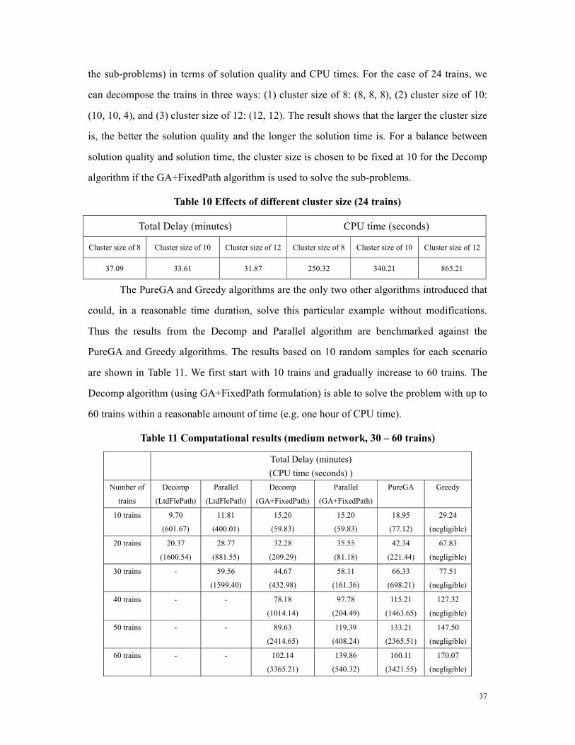
37

the sub-problems) in terms of solution quality and CPU times. For the case of 24 trains, we

can decompose the trains in three ways: (1) cluster size of 8: (8, 8, 8), (2) cluster size of 10:

(10, 10, 4), and (3) cluster size of 12: (12, 12). The result shows that the larger the cluster size

is, the better the solution quality and the longer the solution time is. For a balance between

solution quality and solution time, the cluster size is chosen to be fixed at 10 for the Decomp

algorithm if the GA+FixedPath algorithm is used to solve the sub-problems.

Table 10 Effects of different cluster size (24 trains)

Total Delay (minutes) CPU time (seconds)

Cluster size of 8 Cluster size of 10 Cluster size of 12 Cluster size of 8 Cluster size of 10 Cluster size of 12

37.09 33.61 31.87 250.32 340.21 865.21

The PureGA and Greedy algorithms are the only two other algorithms introduced that

could, in a reasonable time duration, solve this particular example without modifications.

Thus the results from the Decomp and Parallel algorithm are benchmarked against the

PureGA and Greedy algorithms. The results based on 10 random samples for each scenario

are shown in Table 11. We first start with 10 trains and gradually increase to 60 trains. The

Decomp algorithm (using GA+FixedPath formulation) is able to solve the problem with up to

60 trains within a reasonable amount of time (e.g. one hour of CPU time).

Table 11 Computational results (medium network, 30 – 60 trains)

Total Delay (minutes)

(CPU time (seconds) )

Number of

trains

Decomp

(LtdFlePath)

Parallel

(LtdFlePath)

Decomp

(GA+FixedPath)

Parallel

(GA+FixedPath)

PureGA

Greedy

10 trains 9.70

(601.67)

11.81

(400.01)

15.20

(59.83)

15.20

(59.83)

18.95

(77.12)

29.24

(negligible)

20 trains 20.37

(1600.54)

28.77

(881.55)

32.28

(209.29)

35.55

(81.18)

42.34

(221.44)

67.83

(negligible)

30 trains - 59.56

(1599.40)

44.67

(432.98)

58.11

(161.36)

66.33

(698.21)

77.51

(negligible)

40 trains - - 78.18

(1014.14)

97.78

(204.49)

115.21

(1463.65)

127.32

(negligible)

50 trains - - 89.63

(2414.65)

119.39

(408.24)

133.21

(2365.51)

147.50

(negligible)

60 trains - - 102.14

(3365.21)

139.86

(540.32)

160.11

(3421.55)

170.07

(negligible)

38

The relative performances between PureGA and Greedy are consistent with their

performances in the previous example network. By using the LtdFlePath formulation to solve

the sub-problems, we are only able to solve up to 20 and 30 trains for the Decomp and

Parallel algorithms, respectively. The Decomp and Parallel algorithms using the LtdFlePath

formulation return better results than the Decomp and Parallel algorithms using the

GA+FixedPath algorithm for the case of 10 and 20 trains. For the case of 30 trains, it is

interesting to see that the Parallel algorithm using the LtdFlePath formulation returns no

better result than the Decomp and Parallel algorithm using GA+FixedPath algorithm. The

explanation of this is that the cluster size of the Parallel algorithm using the LtdFlePath

formulation is much smaller than the Decomp and Parallel algorithm using the

GA+FixedPath algorithm.

Overall, the Decomp and Parallel algorithm achieves a much smaller delay than the

PureGA and Greedy algorithms. The Decomp algorithm returns a better solution than the

Parallel algorithm does. However because of the ways the sub-problems are integrated, the

Decomp algorithm takes significantly more time to solve the problem than the Parallel

algorithm.

5.3 Large Network

Now we move to a larger sample network, to be more specific, a 49.3-mile long

network from Indio, CA to Colton, CA. The trackage configuration of this network is shown

in Appendix B. The time interval between two consecutive trains in the same direction is

assumed to be uniformly distributed between 14 and 16 minutes. The train speed and train

length are generated as before.

For the Decomp and Parallel algorithm, the cluster size is chosen to be fixed at 6 and

10 (except for the last cluster), respectively. The GA+FixedPath algorithm is used to solve the

sub-problems for both algorithms.

The results based on 20 random samples for each scenario are shown in Table 12. We

first start with 10 trains and gradually increase to 24 trains. The Decomp algorithm is able to

solve the problem with up to 24 trains within a reasonable amount of time.

39

Table 12 Computational results (large network, 10 – 24 trains)

Total Delay (minutes)

(CPU time (seconds) )

Comparison (minutes/minutes)

Decomp Parallel PureGA Greedy Parallel

/Decomp

PureGA

/Decomp

Greedy

/Decomp

10 trains 48.44

(217.9)

57.02

(170.5)

62.12

(587.7)

80.27

(negligible)

1.177 1.282 1.657

12 trains 52.41

(298.0)

61.73

(213.8)

83.36

(1351.9)

101.29

(negligible)

1.178 1.590 1.933

14 trains 66.92

(497.6)

75.46

(263.0)

101.14

(1540.0)

117.45

(negligible)

1.128 1.511 1.755

16 trains 74.96

(716.6)

83.66

(345.1)

110.55

(2057.0)

134.88

(negligible)

1.116 1.475 1.799

18 trains 94.23

(1155.5)

106.46

(449.1)

140.77

(2544.5)

154.54

(negligible)

1.130 1.494 1.640

20 trains 87.40

(1518.5)

101.09

(596.6)

137.64

(2634.0)

153.71

(negligible)

1.157 1.575 1.759

22 trains 100.55

(1992.0)

120.86

(793.0)

170.33

(2818.0)

182.13

(negligible)

1.202 1.694 1.811

24 trains 112.28

(4658.9)

131.31

(978.6)

173.84

(3271.0)

191.18

(negligible)

1.169 1.548 1.703

For the Decomp algorithm, though the problem is decomposed into smaller problems,

the sizes of the sub-problems are not constant. For the case of 18 trains, the average CPU

times to solve sub-problems 1, 2 and 3 are 43.38, 368.69 and 743.25 seconds, respectively. As

expected, the solution quality of the Parallel algorithm is worse than the one for the Decomp

algorithm, since the sub-problems are solved independently. However, the solution time of

the Parallel algorithm is less. And when the number of trains increases, the gap between the

solution times becomes significant.

Table 13 shows the experimental results of the Parallel algorithm for scenarios of 30

and 40 trains. For 30 and 40 trains, neither the Decomp nor PureGA algorithm could solve the

problem in a reasonable amount of time.

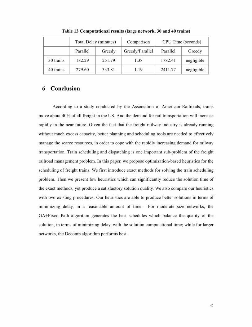
40

Table 13 Computational results (large network, 30 and 40 trains)

Total Delay (minutes) Comparison CPU Time (seconds)

Parallel Greedy Greedy/Parallel Parallel Greedy

30 trains 182.29 251.79 1.38 1782.41 negligible

40 trains 279.60 333.81 1.19 2411.77 negligible

6 Conclusion

According to a study conducted by the Association of American Railroads, trains

move about 40% of all freight in the US. And the demand for rail transportation will increase

rapidly in the near future. Given the fact that the freight railway industry is already running

without much excess capacity, better planning and scheduling tools are needed to effectively

manage the scarce resources, in order to cope with the rapidly increasing demand for railway

transportation. Train scheduling and dispatching is one important sub-problem of the freight

railroad management problem. In this paper, we propose optimization-based heuristics for the

scheduling of freight trains. We first introduce exact methods for solving the train scheduling

problem. Then we present few heuristics which can significantly reduce the solution time of

the exact methods, yet produce a satisfactory solution quality. We also compare our heuristics

with two existing procedures. Our heuristics are able to produce better solutions in terms of

minimizing delay, in a reasonable amount of time. For moderate size networks, the

GA+Fixed Path algorithm generates the best schedules which balance the quality of the

solution, in terms of minimizing delay, with the solution computational time; while for larger

networks, the Decomp algorithm performs best.

41

References

Ahuja, R. K., Cunha, C. B., & Sahin, G. (2005). Network models in railroad planning and scheduling. In H.

J. Greenberg & J. C. Smith (Eds.), TutORials in Operations Research, 54–101

Borndörfer, R. & Schlechte, T. (2008). Solving railway track allocation problems. Operations Research

Proceedings 2007, Kalcsics, J., Nickel, S., Springer-Verlag 117-122.

Cacchiani, V., Caprara, A. & Toth, P. (2010). Scheduling extra freight trains on railway networks.

Transportation Research Part B, 44 (2), 215-231.

Caimi, G. (2009). Algorithmic decision support for train scheduling in a large and highly utilized railway

network, Ph.D. Thesis, ETH Zurich.

Caprara, A., Kroon, L. G., Monaci, M., Peeters, M. & Toth, P. (2006). Passenger railway optimization. In C.

Barnhart & G. Laporte (Eds.), Handbooks in Operations Research and Management Science, 14, 129–187.

Caprara, A., Fischetti, M. & Toth, P. (2002). Modeling and solving the train timetabling problem.

Operations Research, 50 (5), 851–861.

Carey, M. (1994a). A model and strategy for train pathing with choice of lines, platforms, and routes,

Transportation Research Part B, 28 (5), 333-353.

Carey, M. (1994b). Extending a train pathing model from one-way to two-way track, Transportation

Research Part B, 28 (5), 395-400.

Carey M. & Lockwood, D. (1995). A model, algorithms and strategy for train pathing, Journal of

Operation Research Society, 46 (8), 988-1005.

Cordeau, J., Toth, P. & Vigo, D. (1998). A survey of optimization models for train routing and scheduling,

Transporation Science, 32 (4), 380-404.

Corman, F., D’Ariano, A., Pacciarelli D. & Pranzo M. (2010). A tabu search algoritm for rerouting trains

during rail operations, Transportation Research Part B, 44 (1), 175-192.

D’Ariano, A., Pacciarelli, D., & Pranzo, M. (2007). A branch and bound algorithm for scheduling trains in

a railway network. European Journal of Operational Research, 183 (2), 643–657.

Dessouky M., Lu, Q., Zhao, J. & Leachman, R.C. (2006). An exact solution procedure for determining the

optimal dispatching times for complex rail networks, IIE Transaction, 38 (2), 141-152.

Garey, M. R., & Johnson, D. S. (1979). Computers and Intractability: A Guide to Theory of

�P-Completeness, �ew York: Freeman.

42

Higgins, A., Kozan, E., & Ferreira, L. (1996). Optimal scheduling of trains on a single line track,

Transportation Research Part B, 30 (2), 147–161.

Huntley C.L., Brown, D.E., Sappington D.E., & Markowicz, B.P. (1995). Freight routing and scheduling at

CSX transportation, Interfaces, 25 (3), 58-71.

Kraay, D. R., & Harker, P. T. (1995). Real-time scheduling of freight railroads, Transportation Research

Part B, 29 (3), 213–229.

Kraay, D. R., Harker, P. T., & Chen, B. (1991). Optimal pacing of trains in freight railroads: model

formulation and solution, Operations Research, 39 (1), 82–99.

Leachman, R. C. (2002) Los Angeles – inland empire railroad main line advanced planning study,

prepared for the Southern California Association of Governments, contract number 01-077, work element

number 014302, October 1, 2002.

Lu, Q., Dessouky M. & Leachman, R.C. (2004). Modeling train movements through complex rail

networks, ACM Transactions on Modeling and Computer Simulation, 14 (1), 48-75.

Lusby, R.M., Larsen, J., Ehrgott, M. & Ryan, D. (2009). Railway track allocation: models and methods.

OR Spectrum, 31, 1-41.

Ping, L., Axin, N., Limin, J. & Fuzhang, W. (2001). Study on intelligent train dispatching, in Proceedings

of 2001 Intelligent Transportation Systems Conference, 949-953.

Salim, V. & Cai, X. (1995). Scheduling cargo trains using genetic algorithms, in ICEC’95, 224-227.

Tornquist, J., & Persson, J. A. (2007). N-tracked railway traffic re-scheduling during disturbances.

Transportation Research Part B, 41 (3), 342–362.

Suteewong, W. (2006). Algorithms for solving the train dispatching problem for general networks, Ph.D.

Thesis, University of Southern California.

Zhou, X., & Zhong, M. (2007). Single-track train timetabling with guaranteed optimality:

branch-and-bound algorithms with enhanced lower bounds. Transportation Research Part B, 41 (3),

320–341.

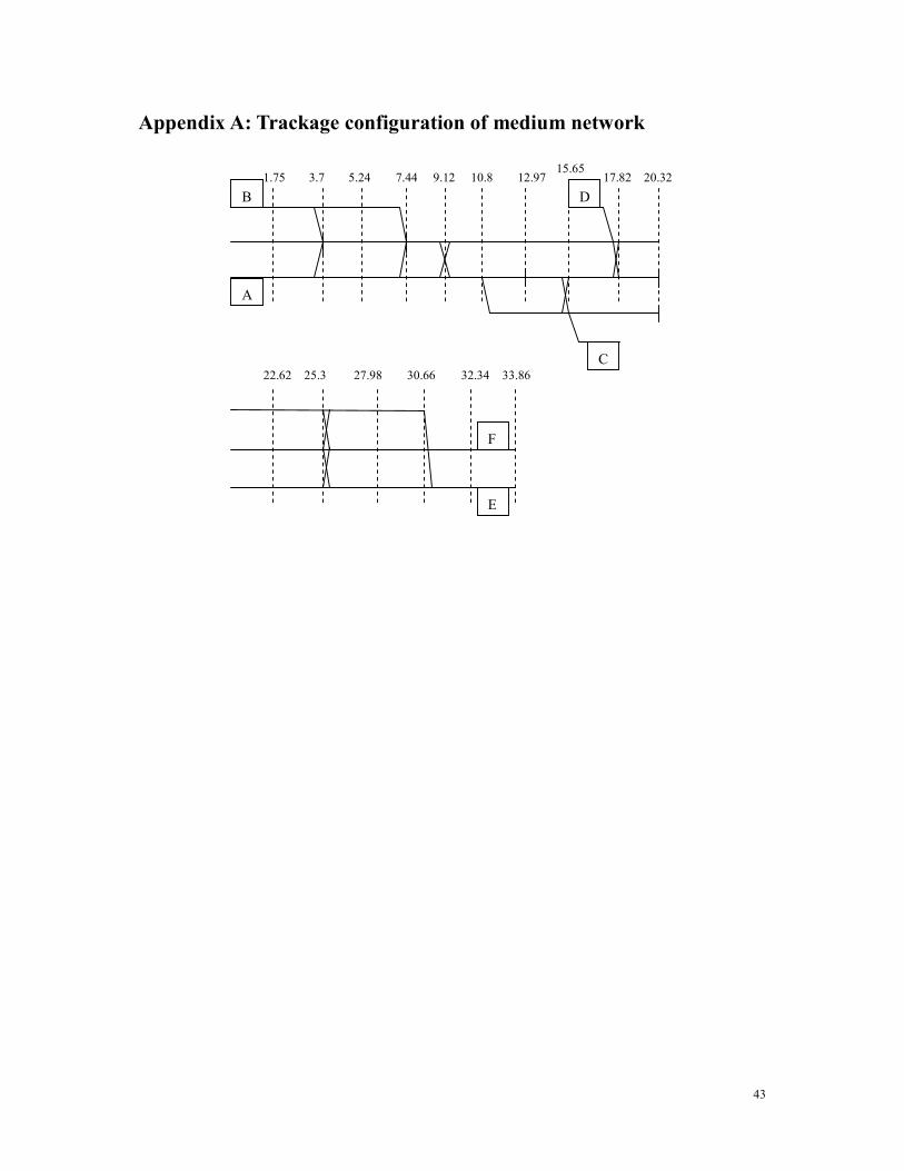
43

Appendix A: Trackage configuration of medium network

A

B

C

D

E

F

1.75 3.7 5.24 7.44 9.12 10.8 12.97 15.65

17.82 20.32

22.62 25.3 27.98 30.66 32.34 33.86

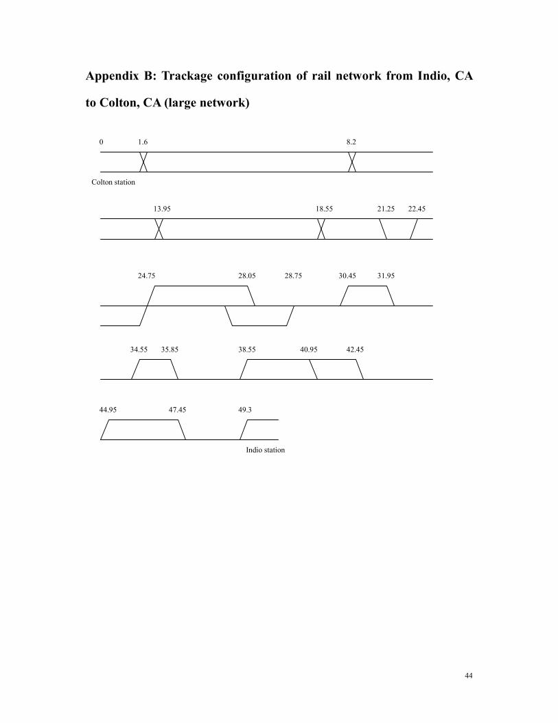
44

Appendix B: Trackage configuration of rail network from Indio, CA

to Colton, CA (large network)

Colton station

0 1.6 8.2

13.95 18.55 21.25 22.45

24.75 28.05 28.75 30.45 31.95

34.55 35.85 38.55 40.95 42.45

44.95 47.45

Indio station

49.3