NASA/TM–2014–216618

Schedule Dissimilarity andStability Metrics for RobustPrecision Air Traffic Operations

D. R. IsaacsonAmes Research Center, Moffett Field, California

A. V. SadovskyAmes Research Center, Moffett Field, California

March 2014

NASA STI Program . . . in Profile

Since its founding, NASA has beendedicated to the advancement ofaeronautics and space science. TheNASA scientific and technicalinformation (STI) program plays a keypart in helping NASA maintain thisimportant role.

The NASA STI Program operatesunder the auspices of the Agency ChiefInformation Officer. It collects,organizes, provides for archiving, anddisseminates NASA’s STI. The NASASTI Program provides access to theNASA Aeronautics and SpaceDatabase and its public interface, theNASA Technical Report Server, thusproviding one of the largest collectionof aeronautical and space science STIin the world. Results are published inboth non-NASA channels and byNASA in the NASA STI Report Series,which includes the following reporttypes:

• TECHNICAL PUBLICATION.Reports of completed research or amajor significant phase of researchthat present the results of NASAprograms and include extensive dataor theoretical analysis. Includescompilations of significant scientificand technical data and informationdeemed to be of continuing referencevalue. NASA counterpart ofpeer-reviewed formal professionalpapers, but having less stringentlimitations on manuscript length andextent of graphic presentations.

• TECHNICAL MEMORANDUM.Scientific and technical findings thatare preliminary or of specializedinterest, e.g., quick release reports,working papers, and bibliographiesthat contain minimal annotation.Does not contain extensive analysis.

• CONTRACTOR REPORT.Scientific and technical findings byNASA-sponsored contractors andgrantees.

• CONFERENCE PUBLICATION.Collected papers from scientific andtechnical conferences, symposia,seminars, or other meetingssponsored or co-sponsored by NASA.

• SPECIAL PUBLICATION.Scientific, technical, or historicalinformation from NASA programs,projects, and missions, oftenconcerned with subjects havingsubstantial public interest.

• TECHNICAL TRANSLATION.English- language translations offoreign scientific and technicalmaterial pertinent to NASA’smission.

Specialized services also includecreating custom thesauri, buildingcustomized databases, and organizingand publishing research results.

For more information about the NASASTI Program, see the following:

• Access the NASA STI program homepage at http://www.sti.nasa.gov

• E-mail your question via the Internetto help@sti.nasa.gov

• Fax your question to the NASA STIHelp Desk at 443-757-5803

• Phone the NASA STI Help Desk at443-757-5802

• Write to:NASA STI Help DeskNASA Center for AeroSpaceInformation7115 Standard DriveHanover, MD 21076–1320

NASA/TM–2014–216618

Schedule Dissimilarity andStability Metrics for RobustPrecision Air Traffic Operations

D. R. IsaacsonAmes Research Center, Moffett Field, California

A. V. SadovskyAmes Research Center, Moffett Field, California

National Aeronautics andSpace Administration

Ames Research CenterMoffett Field, California 94035-0001

March 2014

The use of trademarks or names of manufacturers in this report is for accurate reporting anddoes not constitute an offical endorsement, either expressed or implied, of such products ormanufacturers by the National Aeronautics and Space Administration.

Available from:

NASA Center for AeroSpace Information7115 Standard Drive

Hanover, MD 21076-1320443-757-5802

Abstract

The Next Generation (NextGen) Air Transportation System and theSingle European Sky ATM Research (SESAR) programs aim to overhauland modernize the existing air transportation systems in the UnitedStates and Europe, respectively. The NextGen and SESAR concepts ofoperation leverage procedures based on the Global Positioning Systemand modern aircraft avionics to increase the predictability and reliabilityof air transportation. Air Traffic Operations (ATO) that depend onGPS-based procedures are referred to as Precision Air Traffic Operations(PATO). Such operations, although modeled deterministically in priorwork, remain subject to a number of uncertainties present in the currentsystem, the foremost of which is error in the forecast winds aloft. Asa first step toward scheduling PATO in a stochastic environment, thispaper proposes a precise definition of the stability of a given PATOschedule and a quantitative definition of the dissimilarity between twosuch schedules. These metrics are aimed at recognizing those schedulesand changes to a schedule that may compromise the robustness of thePATO; for example, leading to a loss of aircraft separation or of requiredperformance.

1 Introduction

NextGen and SESAR are envisioned to introduce widespread use of GPS-based procedures called Area Navigation (RNAV) and Required Naviga-tion Performance (RNP) [1]. RNAV and RNP procedures are expectedto increase the predictability of aircraft trajectories and allow for morestrategic application of control strategies for keeping aircraft safely sep-arated and expediting progress toward their destination. However, theenvisioned predictability and efficiency increases depend on aircraft tofollow the prescribed RNAV and RNP procedures. Such operations de-pending on adherence to precisely defined routes of flight are hereaftercalled Precision Air Traffic Operations (PATO).

The problem of PATO scheduling and its constraints are describedin [2]. (Throughout the rest of this paper, the term schedule will, in de-viation from the common use, refer to a vector-valued function of time,defined in detail in a later section.) The mechanisms to be used byair traffic control to separate aircraft conducting PATO are a subjectof current research [3]. However, regardless of the specific form of de-cision support provided to air traffic controllers and flight crews in theconduct of PATO, abrupt, frequent or ill-timed schedule changes can dis-rupt other PATO functions (e.g. providing separation between aircraft).Such disruptions may compromise safety and will likely be deemed un-acceptable by those responsible for the execution of the schedule (i.e.,air traffic controllers and aircraft flight crews). Whatever the form of

1

decision support, the response of the PATO system to the operationaluncertainties (which are described in [2]) will generally entail changesto the schedule. Therefore, to prevent aforementioned disruptions, theseschedule changes must allow the air traffic control (whether human orautomated) and the pilot sufficient time to react.

The purpose of this paper is to propose a quantitative measure of theresponse (manifested as a schedule change) of a PATO system to pertur-bations arising from the operational uncertainties (described in [2] andmodeled here as stochastic perturbations to appropriate input parame-ters1). The primary contribution of this paper is a dissimilarity metricfor an identically-routed schedule pair that allows for consideration ofrobustness in scheduling PATO. This capability is needed to prevent in-herent ATO uncertainties (e.g. wind forecast errors) from causing theaforementioned disruptions. The dissimilarity metric proposed in thispaper will allow for consideration of schedule robustness in two ways:

• as a cost in the objective function of a PATO schedule optimization,and

• as a measure of a given schedule’s sensitivity to the inherent un-certainties.

The computational cost of the methods used to determine a PATO sched-ule will determine how the proposed metric is used in future ATO de-cision support or automation. Given sufficient time and computationalcapabilities, an optimal PATO schedule solution can be sought with anobjective function that reflects schedule robustness and operational pri-orities (e.g. runway utilization and flight efficiency). Lacking sufficientcomputational resources for such an optimization, a given schedule canbe evaluated to determine its sensitivity to inherent ATO uncertaintiesand if the sensitivity of a schedule exceeds a prescribed maximum sensi-tivity, the traffic demand (input) adjusted accordingly as a precautionarymeasure.

The contributions of this paper and the potential future use of thework herein are best understood with knowledge of the PATO schedulingproblem and exposure to the prior work in scheduling (current) ATOand its relevance to PATO. A thorough description of the problem ofscheduling for PATO is included in [2], and a brief review of the formalproblem statement is provided in the following section along with a briefreview of prior research into robust scheduling for PATO. The remainderof this paper is organized to first develop a definition for dissimilaritybetween two PATO schedules and then to provide concise numericalexamples to demonstrate the potential utility of the proposed metrictoward robust NextGen PATO. Lastly, because there will be situations inNextGen, where aircraft will require paths different from those prescribed

1The stochasticity of an input parameter here is a modeling assumption that maybe difficult to test for some parameters and false altogether for others.

2

in a schedule, we present an extension to the proposed metric whichaddresses the case of non identically-routed schedules.

2 Background

This section provides a formal statement of the PATO problem and briefdiscussion of previous research into robust scheduling of PATO.

2.1 Scheduling PATO: problem statement

Derivation of the PATO scheduling problem definition and the enumer-ation of the constraints on PATO scheduling are included in [2]. Oneseeks to route and navigate along the chosen routes a finite set

A = {1, 2, . . . , A}

of A flights in a route network, each flight α ∈ A to go from its ori-gin to its destination, both specified as an input to the problem. Theroute network is modeled as a directed graph, or digraph [4, section A.2],G = (V,E). The vertices v ∈ V are points in a Euclidean space of di-mension 2 or 3, which models the physical airspace, and correspond towaypoints [2] and runways in the airspace. To each edge e = (u, v) ∈ Ecorresponds a rectifiable curve [5, section 4.6-9] which, therefore, has awell-defined arc length. Henceforth, an edge e ∈ E will be identifiedwith the corresponding curve. A graph G = (V,E) with this additionalgeometric setting will be called an airspace graph.

Each aircraft is modeled as a point moving along an edge of G. Thus,to each aircraft α we associate a path in the graph G. Such a path, be-ing a concatenation of continuous and piecewise differentiable curves, isitself such a curve. Once an arc length coordinate s(α) is introduced onthis curve for aircraft α, the value of this coordinate at time t completelyspecifies the physical position of agent α at time t. It follows immediatelythat the time derivative of s(α)(t) gives the agent’s instantaneous groundspeed along its path. The formal problem statement is as follows [2]:

Given

• for each α ∈ A a path (parameterized by arc length s(α)) in G,

• the full set of constraints (e.g. separation minima) on the s(α)(t)’sand on their time derivatives (e.g. airspeed restrictions),

• a control dynamical law for the evolution of the s(α)(t)’s, and

• an objective function of the vector-valued function (s(α)(t))α∈A oftime,

3

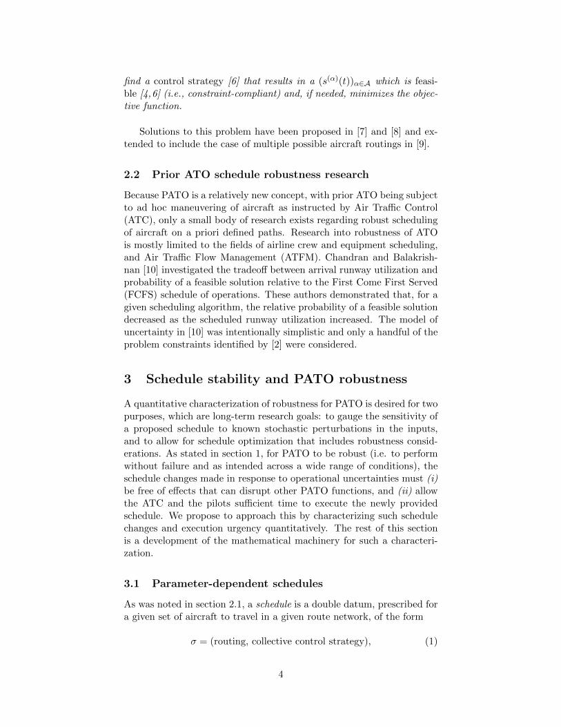
find a control strategy [6] that results in a (s(α)(t))α∈A which is feasi-ble [4,6] (i.e., constraint-compliant) and, if needed, minimizes the objec-tive function.

Solutions to this problem have been proposed in [7] and [8] and ex-tended to include the case of multiple possible aircraft routings in [9].

2.2 Prior ATO schedule robustness research

Because PATO is a relatively new concept, with prior ATO being subjectto ad hoc maneuvering of aircraft as instructed by Air Traffic Control(ATC), only a small body of research exists regarding robust schedulingof aircraft on a priori defined paths. Research into robustness of ATOis mostly limited to the fields of airline crew and equipment scheduling,and Air Traffic Flow Management (ATFM). Chandran and Balakrish-nan [10] investigated the tradeoff between arrival runway utilization andprobability of a feasible solution relative to the First Come First Served(FCFS) schedule of operations. These authors demonstrated that, for agiven scheduling algorithm, the relative probability of a feasible solutiondecreased as the scheduled runway utilization increased. The model ofuncertainty in [10] was intentionally simplistic and only a handful of theproblem constraints identified by [2] were considered.

3 Schedule stability and PATO robustness

A quantitative characterization of robustness for PATO is desired for twopurposes, which are long-term research goals: to gauge the sensitivity ofa proposed schedule to known stochastic perturbations in the inputs,and to allow for schedule optimization that includes robustness consid-erations. As stated in section 1, for PATO to be robust (i.e. to performwithout failure and as intended across a wide range of conditions), theschedule changes made in response to operational uncertainties must (i)be free of effects that can disrupt other PATO functions, and (ii) allowthe ATC and the pilots sufficient time to execute the newly providedschedule. We propose to approach this by characterizing such schedulechanges and execution urgency quantitatively. The rest of this sectionis a development of the mathematical machinery for such a characteri-zation.

3.1 Parameter-dependent schedules

As was noted in section 2.1, a schedule is a double datum, prescribed fora given set of aircraft to travel in a given route network, of the form

σ = (routing, collective control strategy), (1)

4

where the routing refers to a function mapping each aircraft α ∈ A inthe given operation to a path in the route network, and the collectivecontrol strategy is a vector

u(t) =(u(α)(t)

)α∈A

that prescribes the motion for all aircraft simultaneously, with the u(α)’sbeing the control variables in the state equations [5, section 11.8-1(a)] ofthis motion. If inertia is neglected in the model provided by the stateequations, then the u(α)’s are typically the speeds; otherwise, if inertia isincluded, the u(α)’s are typically the accelerations, while the speeds andthe arc length coordinates of the aircraft are the state variables. Thetheory developed in this paper is applicable to both cases, and in bothcases rests on the following assumption.

Assumption 3.1. The speeds appearing, whether as state variables oras control variables, in the state equations and in the rest of the modelare the true air speeds.

One consequence of this assumption is that one cannot, withoutknowing the wind field, calculate the ground speeds and flight timesof the aircraft.

Both constituent components of a schedule (1), the routing and thecontrol strategy, are functions of a parameter that takes values in someparameter space P (e.g., a suitable class of wind vector fields on the givenairspace), which is a subset of a vector space with some norm [5, section14.2-5], denoted || · ||. If a schedule σ corresponds to a parameter valuep ∈ P, this correspondence will sometimes be made explicit using thenotation

σ = σ(p)

As previously stated, schedule changes must not disrupt other PATOfunctions. Intuitively, we will consider a schedule stable at a given pa-rameter value p (or, briefly, stable at p) if by small perturbations to p onecannot with high probability cause “large changes in the schedule (i.e.schedule changes that disrupt other PATO functions). A mathematicalmodel of this intuition requires, in particular, a function that measuresthe dissimilarity between a pair of schedules. A general class of suchfunctions is constructed below, in section 3.2, and has the behavior ofwhat is called in mathematics a metric or a distance function [5, defini-tion 12-5.2].

3.2 Definition of dissimilarity for identically routed sched-ule pairs

In this section, we define quantitatively the dissimilarity between twosolutions, σ1 and σ2, to the PATO scheduling problem [2]. The followingdefinition will be instrumental to this discussion.

5

Definition 3.1. (a) Two schedules that have the same route network,aircraft set A, and separation and speed constraints, and differ only inthe parameter value, will be called a schedule pair. (b) A schedule pairwith the same routing is said to be identically routed.

In this paper, we consider those schedule pairs that are identicallyrouted. A generalization to the case when a perturbation to the param-eter changes the routing, discussed briefly in Section 5 below, is a topicfor future research.

The intuition for the definition of dissimilarity is as follows. An iden-tically routed schedule pair will be thought the more dissimilar, the more“substantial” the operational change from one to the other. A changein the speed advisory v(α) for an individual aircraft α is considered themore “substantial”2 the greater the volume of instructions is to be issuedby the ATC and executed by the pilot. Thus, at each point s along theaircraft’s path, the qualitative form of the “instantaneous dissimiliarity”between the two speed advisories v(σ1;α)(s), v(σ2;α)(s) furnished for α bythe two respective schedules σ1, σ2 has the qualitative form(

the absolute difference between v(σ1;α)(s) and v(σ2;α)(s)). (2)

Once a mathematical definition for (2) is stated, the individual, foraircraft α, dissimilarity between σ1 and σ2 can be defined as the integralof (2) with respect to the arc length coordinate of the flight path of α,taken along the entire path. The dissimilarity d(σ1, σ2) (total, for theentire operation) between schedules σ1 and σ2 will be defined as thesummation over all α of the these integrals.

The quantity in (2) can be defined as a suitable continuous and non-decreasing function of the absolute difference

|v(σ1;α)(s)− v(σ2;α)(s)|.

To guarantee certain smoothness, this function will be chosen as one thatsquares its argument. Finally, the arc length coordinate along the pathof aircraft α varies from a value denoted s(ENT ;α) (entrance) to a valuedenoted a value denoted s(EXIT ;α) (exit).

The resulting definition of the dissimilarity of an identically routedschedule pair σ1, σ2 is

d(σ1, σ2) =

√√√√∑α

{∫ s(EXIT ;α)

s(ENT ;α)

[v(σ1;α)(s)− v(σ2;α)(s)

]2ds

}(3)

It can be proved that, on a class of schedules where each two form aschedule pair (see definition 3.1, above) and are identically routed, the

2I.e., requiring a more substantial or labor-intensive revision of the entire operationin question.

6

dissimilarity function d(·, ·) is a metric in the sense of [5, definition 12-5.2]3, and will be used in the definition of schedule stability (see Section3.4.1).

3.3 Numerical examples of pairwise dissimilarities in a setof schedules

3.3.1 Two schedules for two aircraft whose rectilinear pathscross perpendicularly

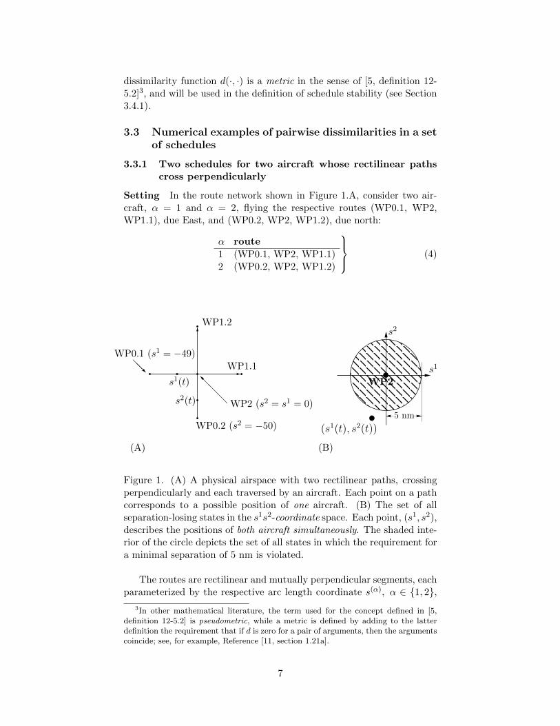
Setting In the route network shown in Figure 1.A, consider two air-craft, α = 1 and α = 2, flying the respective routes (WP0.1, WP2,WP1.1), due East, and (WP0.2, WP2, WP1.2), due north:

α route

1 (WP0.1, WP2, WP1.1)2 (WP0.2, WP2, WP1.2)

(4)

(A)

WP0.1 (s1 = −49)@@R

WP0.2 (s2 = −50)

WP1.1

WP1.2

WP2 (s2 = s1 = 0)@@@Is1(t)

s2(t)

(B)

WP2

5 nm

s1

s2

(s1(t), s2(t))

Figure 1. (A) A physical airspace with two rectilinear paths, crossingperpendicularly and each traversed by an aircraft. Each point on a pathcorresponds to a possible position of one aircraft. (B) The set of allseparation-losing states in the s1s2-coordinate space. Each point, (s1, s2),describes the positions of both aircraft simultaneously. The shaded inte-rior of the circle depicts the set of all states in which the requirement fora minimal separation of 5 nm is violated.

The routes are rectilinear and mutually perpendicular segments, eachparameterized by the respective arc length coordinate s(α), α ∈ {1, 2},

3In other mathematical literature, the term used for the concept defined in [5,definition 12-5.2] is pseudometric, while a metric is defined by adding to the latterdefinition the requirement that if d is zero for a pair of arguments, then the argumentscoincide; see, for example, Reference [11, section 1.21a].

7

as shown in Figure 1.A. Assume the required separation for the twoaircraft, regardless of relative position, is 5 nm.

The coordinate space for this air traffic model is the set of all pairs(s1, s2) with s1 ≥ −49, s2 ≥ −50, with the crossing point, WP2, at theorigin: s1 = s2 = 0. The set of all coordinate pairs (s1, s2) that havethe two aircraft within 5 nm of each other, i.e. that lose separation, isshown in Figure 1.B) as the shaded interior of a circle centered at theorigin and with radius 5; for detailed derivations, see [7, 9].

Suppose that the aircraft are initially at WP0.1 (s10 = −49) nm andWP0.2 (s20 = −50) nm, respectively, i.e. are in the initial state

s0 =(s10, s

20

)= (−49,−50)

in the s1s2-coordinate space, and impose the following feasible speedrange constraint:

Each aircraft has minimal feasible airspeed V min = 420 kts andmaximal feasible airspeed V max = 475 kts.

}(5)

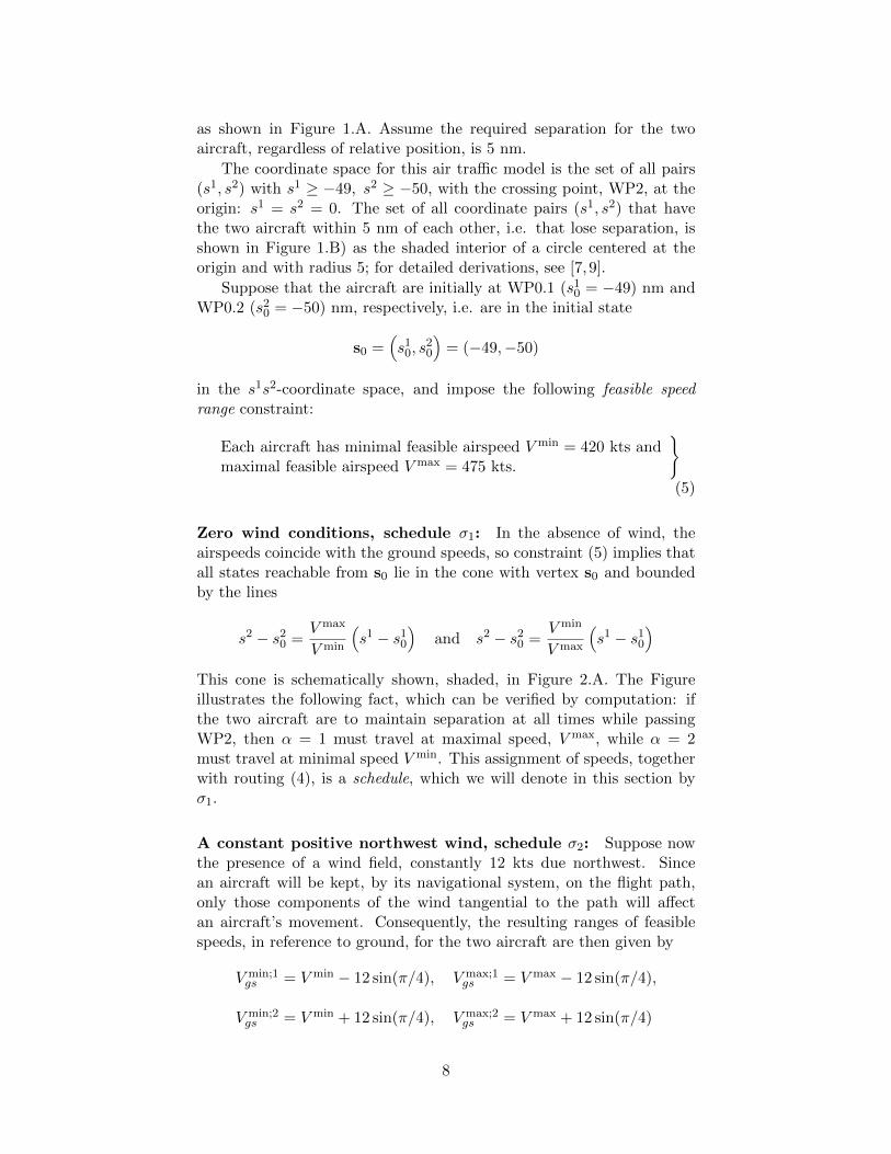
Zero wind conditions, schedule σ1: In the absence of wind, theairspeeds coincide with the ground speeds, so constraint (5) implies thatall states reachable from s0 lie in the cone with vertex s0 and boundedby the lines

s2 − s20 =V max

V min

(s1 − s10

)and s2 − s20 =

V min

V max

(s1 − s10

)This cone is schematically shown, shaded, in Figure 2.A. The Figureillustrates the following fact, which can be verified by computation: ifthe two aircraft are to maintain separation at all times while passingWP2, then α = 1 must travel at maximal speed, V max, while α = 2must travel at minimal speed V min. This assignment of speeds, togetherwith routing (4), is a schedule, which we will denote in this section byσ1.

A constant positive northwest wind, schedule σ2: Suppose nowthe presence of a wind field, constantly 12 kts due northwest. Sincean aircraft will be kept, by its navigational system, on the flight path,only those components of the wind tangential to the path will affectan aircraft’s movement. Consequently, the resulting ranges of feasiblespeeds, in reference to ground, for the two aircraft are then given by

V min;1gs = V min − 12 sin(π/4), V max;1

gs = V max − 12 sin(π/4),

V min;2gs = V min + 12 sin(π/4), V max;2

gs = V max + 12 sin(π/4)

8

(A)

s1

s2

just feasible@@@I

s0

slope V min/V max

6

slope V max/V min

HHHHj

(B)

s1

s2

s0

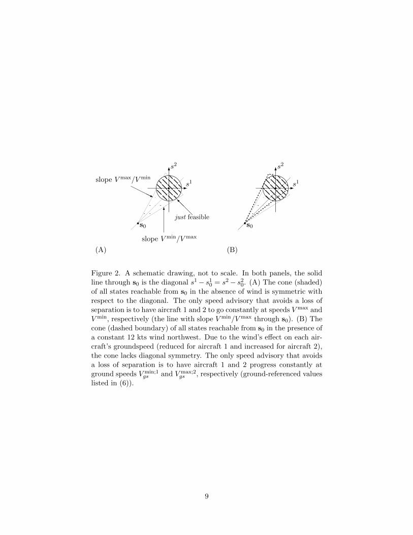
Figure 2. A schematic drawing, not to scale. In both panels, the solidline through s0 is the diagonal s1− s10 = s2− s20. (A) The cone (shaded)of all states reachable from s0 in the absence of wind is symmetric withrespect to the diagonal. The only speed advisory that avoids a loss ofseparation is to have aircraft 1 and 2 to go constantly at speeds V max andV min, respectively (the line with slope V min/V max through s0). (B) Thecone (dashed boundary) of all states reachable from s0 in the presence ofa constant 12 kts wind northwest. Due to the wind’s effect on each air-craft’s groundspeed (reduced for aircraft 1 and increased for aircraft 2),the cone lacks diagonal symmetry. The only speed advisory that avoidsa loss of separation is to have aircraft 1 and 2 progress constantly atground speeds V min;1

gs and V max;2gs , respectively (ground-referenced values

listed in (6)).

9

which have the following approximate values:

α V (min;α) V (max;α)

1 411.52 466.522 428.49 483.49

(6)

As is illustrated in Figure 2.B (and can be verified numerically), theonly speed advisory that avoids a loss of separation is to have aircraft 1and 2 to go constantly at ground speeds V min;1 and V max;2, respectively(values listed in (6)). This schedule will be denoted by σ2. In termsof airspeeds, σ2 prescribes that aircraft 1 and 2 go at speeds V min andV max, respectively.

Dissimilarity between σ1 and σ2 The dissimilarity (3) between thetwo schedules is, therefore,√∫ 0

−49[V max − V min]2 ds1 +

∫ 0

−50[V min − V max]2 ds2

.= 547.24 (7)

Figure 2.A shows that any increase, however slight, in the slopes ofthe lines that bound the shaded cone will make the speed advisory inσ1 impossible to execute without losing separation. Consequently, thefollowing observation (used below) holds for this example:

Remark 3.1. With a constant wind northwest, of a magnitude strictlybetween 0 kts and 12 kts (see Figure 2B), schedule σ1 is infeasible.

3.3.2 Three schedules for two aircraft on a simple route net-work

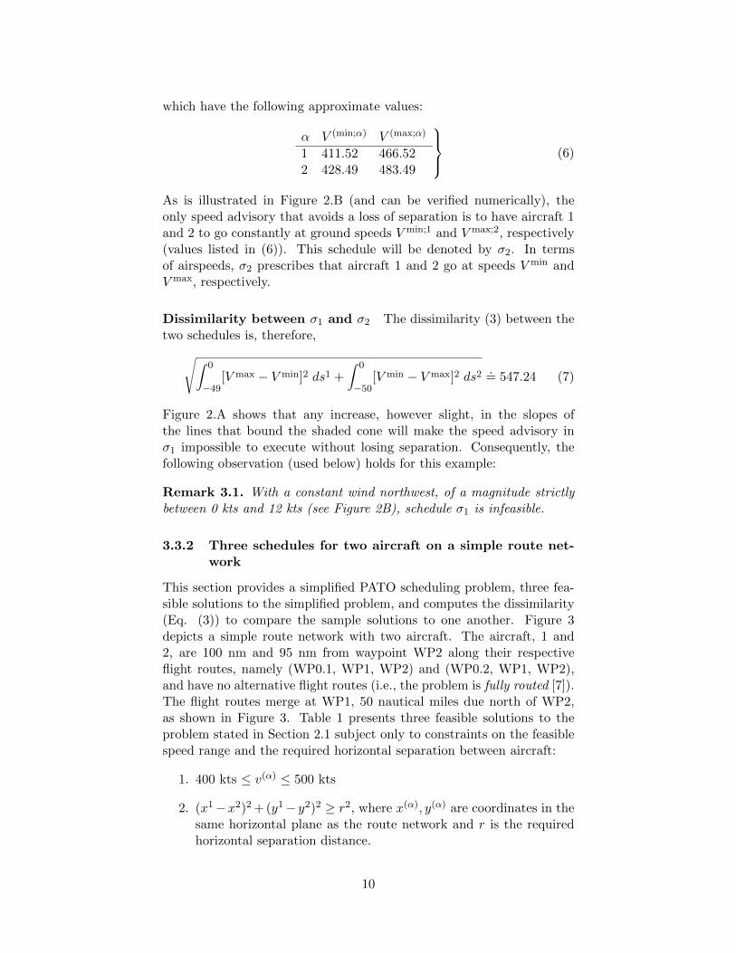
This section provides a simplified PATO scheduling problem, three fea-sible solutions to the simplified problem, and computes the dissimilarity(Eq. (3)) to compare the sample solutions to one another. Figure 3depicts a simple route network with two aircraft. The aircraft, 1 and2, are 100 nm and 95 nm from waypoint WP2 along their respectiveflight routes, namely (WP0.1, WP1, WP2) and (WP0.2, WP1, WP2),and have no alternative flight routes (i.e., the problem is fully routed [7]).The flight routes merge at WP1, 50 nautical miles due north of WP2,as shown in Figure 3. Table 1 presents three feasible solutions to theproblem stated in Section 2.1 subject only to constraints on the feasiblespeed range and the required horizontal separation between aircraft:

1. 400 kts ≤ v(α) ≤ 500 kts

2. (x1−x2)2 + (y1− y2)2 ≥ r2, where x(α), y(α) are coordinates in thesame horizontal plane as the route network and r is the requiredhorizontal separation distance.

10

α = 1 α = 2

s1 = −100����

s2 = −95@

@@I

s1 = s2 = 0 -

s1 = s2 = −50 ����

WP0.1 WP0.2

WP2

WP1

Figure 3. A simple route network with two aircraft

The values of the pairwise dissimilarities (3) for the three sampleschedules are approximately:

d(σ1, σ2) ≈ 5.91 (8)

d(σ2, σ3) ≈ 3.58 (9)

d(σ1, σ3) ≈ 7.16 (10)

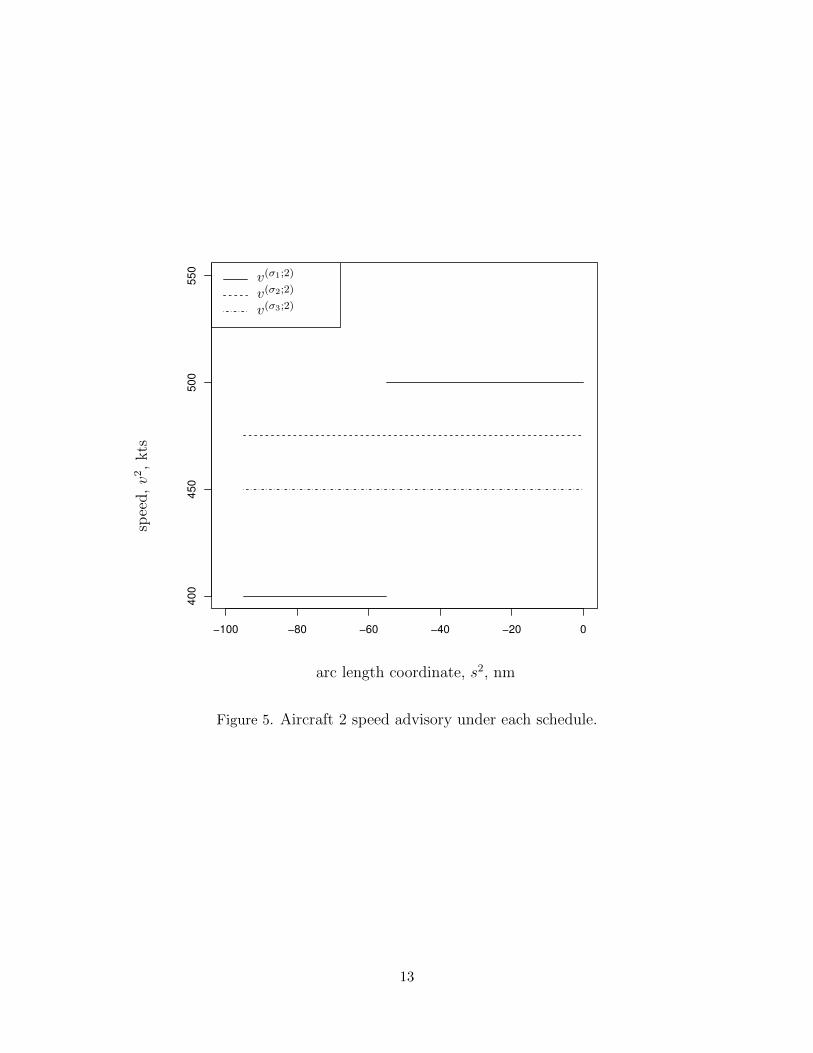
The dissimilarities (8), (9), (10) imply that the schedule pair (σ1, σ3)is more dissimilar than is the pair (σ2, σ3). These results match the fol-lowing intuition. Schedules σ2 and σ3 differ only by 25 kts along theentire flight route of each aircraft (see Figures 4 and 5). Schedules σ1and σ3 not only exhibit greater differences in speeds, but also prescribedifferent orders of aircraft arrival at WP2 (see Figure 3). Changes inaircraft arrival order indicate a significantly different schedule to the airtraffic control and to pilots, as separation standards may differ and pi-lot visual acquisition of leading aircraft may be required. While aircraftorder is not considered in schedule dissimilarity (3), reordering in con-gested terminal airspace would typically require large speed changes (orrerouting).

11

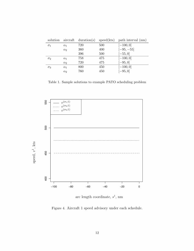
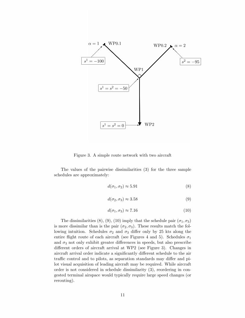
solution aircraft duration(s) speed(kts) path interval (nm)

σ1 α1 720 500 [−100, 0]α2 360 400 [−95,−55]

396 500 [−55, 0]

σ2 α1 758 475 [−100, 0]α2 720 475 [−95, 0]

σ3 α1 800 450 [−100, 0]α2 760 450 [−95, 0]

Table 1. Sample solutions to example PATO scheduling problem

−100 −80 −60 −40 −20 0

40

04

50

50

05

50

v(σ1;1)

v(σ2;1)

v(σ3;1)

arc length coordinate, s1, nm

speed,v1,kts

Figure 4. Aircraft 1 speed advisory under each schedule.

12

−100 −80 −60 −40 −20 0

40

04

50

50

05

50

v(σ1;2)

v(σ2;2)

v(σ3;2)

arc length coordinate, s2, nm

speed,v2,kts

Figure 5. Aircraft 2 speed advisory under each schedule.

13

3.4 Schedule stability and robustness

3.4.1 Schedule stability to stochastic perturbations

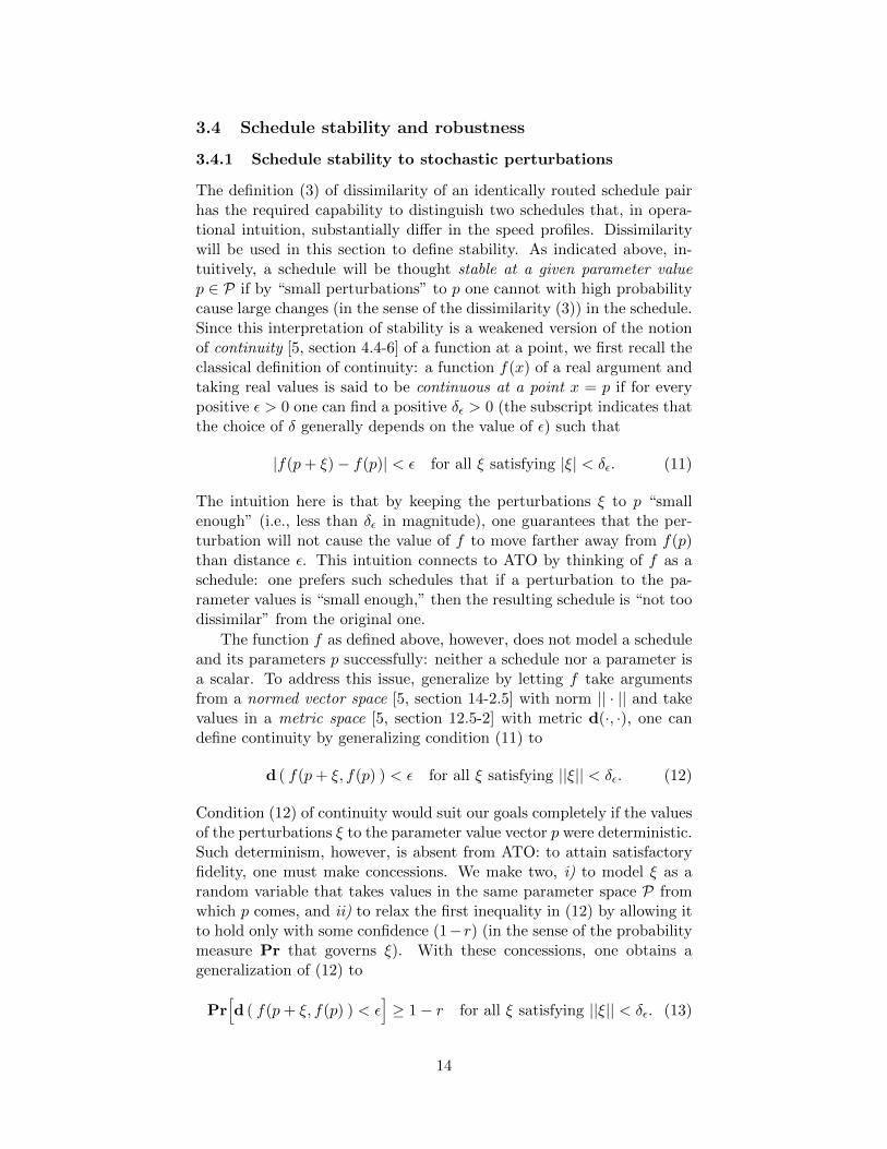
The definition (3) of dissimilarity of an identically routed schedule pairhas the required capability to distinguish two schedules that, in opera-tional intuition, substantially differ in the speed profiles. Dissimilaritywill be used in this section to define stability. As indicated above, in-tuitively, a schedule will be thought stable at a given parameter valuep ∈ P if by “small perturbations” to p one cannot with high probabilitycause large changes (in the sense of the dissimilarity (3)) in the schedule.Since this interpretation of stability is a weakened version of the notionof continuity [5, section 4.4-6] of a function at a point, we first recall theclassical definition of continuity: a function f(x) of a real argument andtaking real values is said to be continuous at a point x = p if for everypositive ε > 0 one can find a positive δε > 0 (the subscript indicates thatthe choice of δ generally depends on the value of ε) such that

|f(p+ ξ)− f(p)| < ε for all ξ satisfying |ξ| < δε. (11)

The intuition here is that by keeping the perturbations ξ to p “smallenough” (i.e., less than δε in magnitude), one guarantees that the per-turbation will not cause the value of f to move farther away from f(p)than distance ε. This intuition connects to ATO by thinking of f as aschedule: one prefers such schedules that if a perturbation to the pa-rameter values is “small enough,” then the resulting schedule is “not toodissimilar” from the original one.

The function f as defined above, however, does not model a scheduleand its parameters p successfully: neither a schedule nor a parameter isa scalar. To address this issue, generalize by letting f take argumentsfrom a normed vector space [5, section 14-2.5] with norm || · || and takevalues in a metric space [5, section 12.5-2] with metric d(·, ·), one candefine continuity by generalizing condition (11) to

d ( f(p+ ξ, f(p) ) < ε for all ξ satisfying ||ξ|| < δε. (12)

Condition (12) of continuity would suit our goals completely if the valuesof the perturbations ξ to the parameter value vector p were deterministic.Such determinism, however, is absent from ATO: to attain satisfactoryfidelity, one must make concessions. We make two, i) to model ξ as arandom variable that takes values in the same parameter space P fromwhich p comes, and ii) to relax the first inequality in (12) by allowing itto hold only with some confidence (1−r) (in the sense of the probabilitymeasure Pr that governs ξ). With these concessions, one obtains ageneralization of (12) to

Pr[d ( f(p+ ξ, f(p) ) < ε

]≥ 1− r for all ξ satisfying ||ξ|| < δε. (13)

14

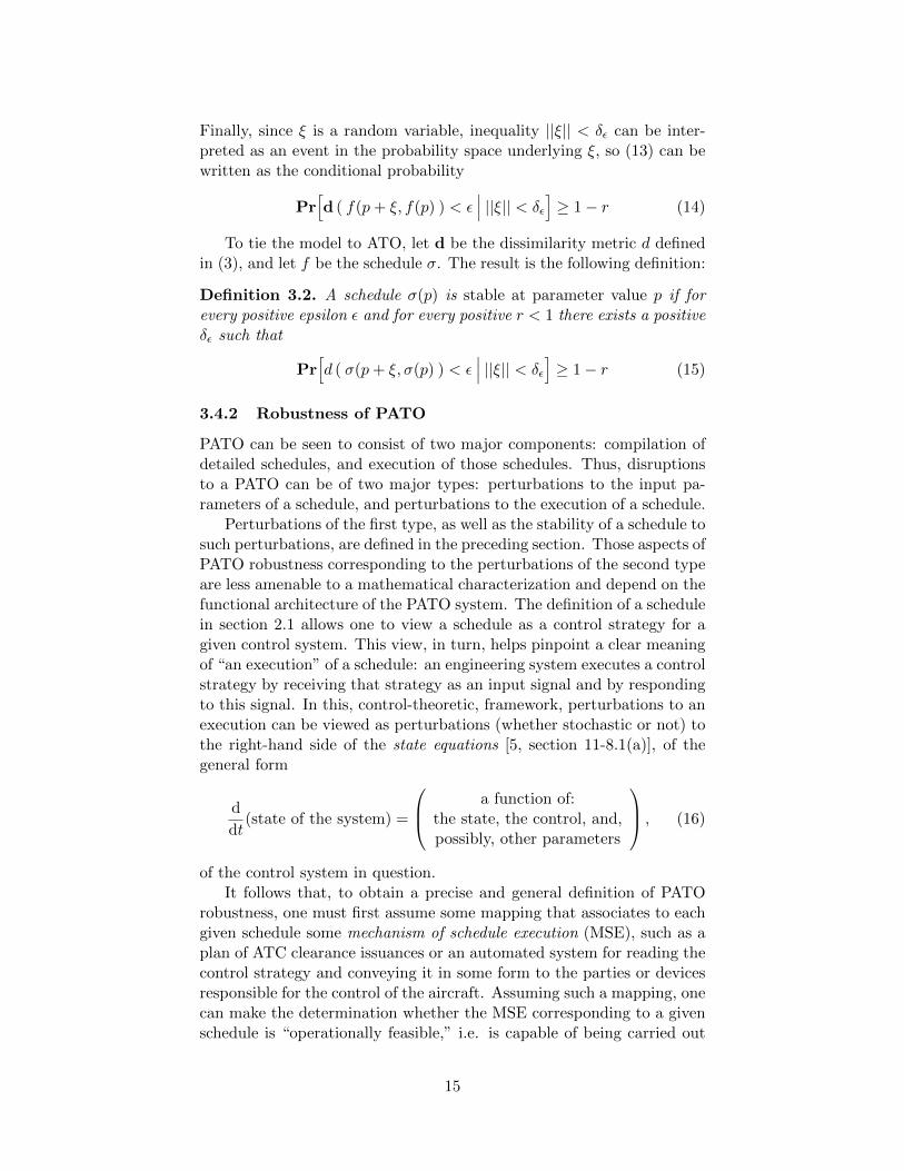
Finally, since ξ is a random variable, inequality ||ξ|| < δε can be inter-preted as an event in the probability space underlying ξ, so (13) can bewritten as the conditional probability

Pr[d ( f(p+ ξ, f(p) ) < ε

∣∣∣ ||ξ|| < δε]≥ 1− r (14)

To tie the model to ATO, let d be the dissimilarity metric d definedin (3), and let f be the schedule σ. The result is the following definition:

Definition 3.2. A schedule σ(p) is stable at parameter value p if forevery positive epsilon ε and for every positive r < 1 there exists a positiveδε such that

Pr[d ( σ(p+ ξ, σ(p) ) < ε

∣∣∣ ||ξ|| < δε]≥ 1− r (15)

3.4.2 Robustness of PATO

PATO can be seen to consist of two major components: compilation ofdetailed schedules, and execution of those schedules. Thus, disruptionsto a PATO can be of two major types: perturbations to the input pa-rameters of a schedule, and perturbations to the execution of a schedule.

Perturbations of the first type, as well as the stability of a schedule tosuch perturbations, are defined in the preceding section. Those aspects ofPATO robustness corresponding to the perturbations of the second typeare less amenable to a mathematical characterization and depend on thefunctional architecture of the PATO system. The definition of a schedulein section 2.1 allows one to view a schedule as a control strategy for agiven control system. This view, in turn, helps pinpoint a clear meaningof “an execution” of a schedule: an engineering system executes a controlstrategy by receiving that strategy as an input signal and by respondingto this signal. In this, control-theoretic, framework, perturbations to anexecution can be viewed as perturbations (whether stochastic or not) tothe right-hand side of the state equations [5, section 11-8.1(a)], of thegeneral form

d

dt(state of the system) =

a function of:the state, the control, and,possibly, other parameters

, (16)

of the control system in question.It follows that, to obtain a precise and general definition of PATO

robustness, one must first assume some mapping that associates to eachgiven schedule some mechanism of schedule execution (MSE), such as aplan of ATC clearance issuances or an automated system for reading thecontrol strategy and conveying it in some form to the parties or devicesresponsible for the control of the aircraft. Assuming such a mapping, onecan make the determination whether the MSE corresponding to a givenschedule is “operationally feasible,” i.e. is capable of being carried out

15

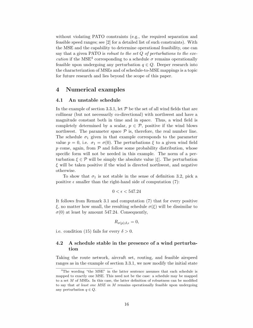
without violating PATO constraints (e.g., the required separation andfeasible speed ranges; see [2] for a detailed list of such constraints). Withthe MSE and the capability to determine operational feasibility, one cansay that a given PATO is robust to the set Q of perturbations to the exe-cution if the MSE4 corresponding to a schedule σ remains operationallyfeasible upon undergoing any perturbation q ∈ Q. Deeper research intothe characterization of MSEs and of schedule-to-MSE mappings is a topicfor future research and lies beyond the scope of this paper.

4 Numerical examples

4.1 An unstable schedule

In the example of section 3.3.1, let P be the set of all wind fields that arecollinear (but not necessarily co-directional) with northwest and have amagnitude constant both in time and in space. Thus, a wind field iscompletely determined by a scalar, p ∈ P, positive if the wind blowsnorthwest. The parameter space P is, therefore, the real number line.The schedule σ1 given in that example corresponds to the parametervalue p = 0, i.e. σ1 = σ(0). The perturbations ξ to a given wind fieldp come, again, from P and follow some probability distribution, whosespecific form will not be needed in this example. The norm of a per-turbation ξ ∈ P will be simply the absolute value |ξ|. The perturbationξ will be taken positive if the wind is directed northwest, and negativeotherwise.

To show that σ1 is not stable in the sense of definition 3.2, pick apositive ε smaller than the right-hand side of computation (7):

0 < ε < 547.24

It follows from Remark 3.1 and computation (7) that for every positiveξ, no matter how small, the resulting schedule σ(ξ) will be dissimilar toσ(0) at least by amount 547.24. Consequently,

Rσ(p);δ,ε = 0,

i.e. condition (15) fails for every δ > 0.

4.2 A schedule stable in the presence of a wind perturba-tion

Taking the route network, aircraft set, routing, and feasible airspeedranges as in the example of section 3.3.1, we now modify the initial state

4The wording “the MSE” in the latter sentence assumes that each schedule ismapped to exactly one MSE. This need not be the case: a schedule may be mappedto a set M of MSEs. In this case, the latter definition of robustness can be modifiedto say that at least one MSE in M remains operationally feasible upon undergoingany perturbation q ∈ Q.

16

s0

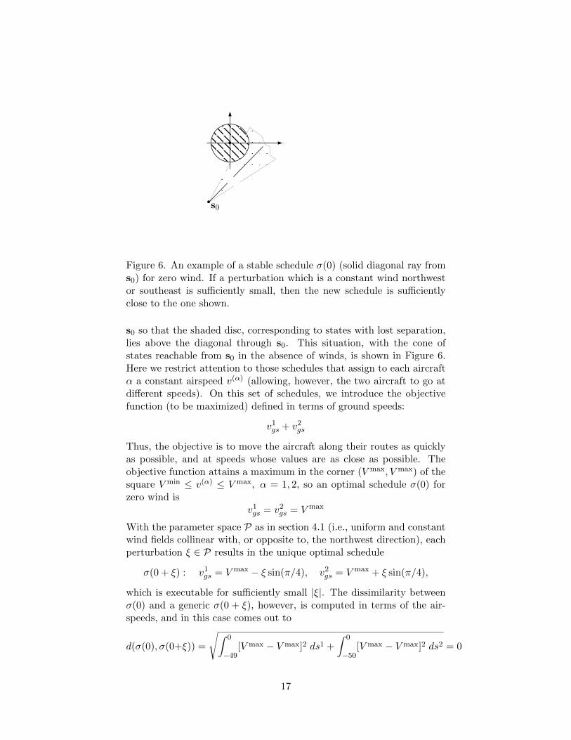
Figure 6. An example of a stable schedule σ(0) (solid diagonal ray froms0) for zero wind. If a perturbation which is a constant wind northwestor southeast is sufficiently small, then the new schedule is sufficientlyclose to the one shown.

s0 so that the shaded disc, corresponding to states with lost separation,lies above the diagonal through s0. This situation, with the cone ofstates reachable from s0 in the absence of winds, is shown in Figure 6.Here we restrict attention to those schedules that assign to each aircraftα a constant airspeed v(α) (allowing, however, the two aircraft to go atdifferent speeds). On this set of schedules, we introduce the objectivefunction (to be maximized) defined in terms of ground speeds:

v1gs + v2gs

Thus, the objective is to move the aircraft along their routes as quicklyas possible, and at speeds whose values are as close as possible. Theobjective function attains a maximum in the corner (V max, V max) of thesquare V min ≤ v(α) ≤ V max, α = 1, 2, so an optimal schedule σ(0) forzero wind is

v1gs = v2gs = V max

With the parameter space P as in section 4.1 (i.e., uniform and constantwind fields collinear with, or opposite to, the northwest direction), eachperturbation ξ ∈ P results in the unique optimal schedule

σ(0 + ξ) : v1gs = V max − ξ sin(π/4), v2gs = V max + ξ sin(π/4),

which is executable for sufficiently small |ξ|. The dissimilarity betweenσ(0) and a generic σ(0 + ξ), however, is computed in terms of the air-speeds, and in this case comes out to

d(σ(0), σ(0+ξ)) =

√∫ 0

−49[V max − V max]2 ds1 +

∫ 0

−50[V max − V max]2 ds2 = 0

17

It follows that Rσ(p);δ,ε = 1 for all sufficiently small δ > 0, and conse-quently schedule σ(0) is stable (at parameter value p = 0).

4.3 A schedule stable in the presence of a control execu-tion timing perturbation

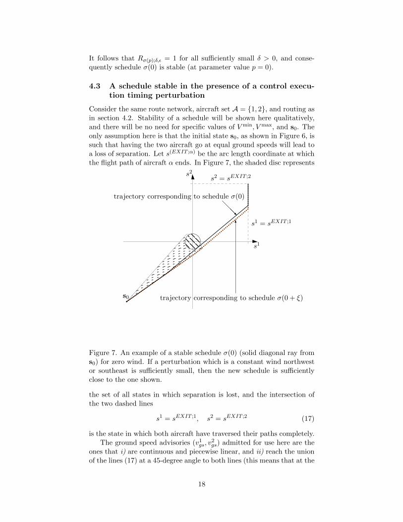
Consider the same route network, aircraft set A = {1, 2}, and routing asin section 4.2. Stability of a schedule will be shown here qualitatively,and there will be no need for specific values of V min, V max, and s0. Theonly assumption here is that the initial state s0, as shown in Figure 6, issuch that having the two aircraft go at equal ground speeds will lead toa loss of separation. Let s(EXIT ;α) be the arc length coordinate at whichthe flight path of aircraft α ends. In Figure 7, the shaded disc represents

s0

s1 = sEXIT ;1

s1

s2 = sEXIT ;2s2

trajectory corresponding to schedule σ(0)@@@R

trajectory corresponding to schedule σ(0 + ξ)

6

Figure 7. An example of a stable schedule σ(0) (solid diagonal ray froms0) for zero wind. If a perturbation which is a constant wind northwestor southeast is sufficiently small, then the new schedule is sufficientlyclose to the one shown.

the set of all states in which separation is lost, and the intersection ofthe two dashed lines

s1 = sEXIT ;1, s2 = sEXIT ;2 (17)

is the state in which both aircraft have traversed their paths completely.The ground speed advisories (v1gs, v

2gs) admitted for use here are the

ones that i) are continuous and piecewise linear, and ii) reach the unionof the lines (17) at a 45-degree angle to both lines (this means that at the

18

instant when a first aircraft reaches the end of its path, the two aircraftare going at the same ground speed). Recall that each speed advisory,(v1gs(t), v

2gs(t)), gives rise to a trajectory (s1(t), s2(t)) in the arc length

coordinate space; this trajectory is the solution to the ODE system

ds(α)

dt= v(α)gs , α ∈ A

with the initial condition

(s1(0), s2(0)) = s0

The objective function used here is

(percentage of the entire trajectory length parallel to the diagonal)

(#cusps in a speed advisory)(18)

The parameter here is control latency (see [2, appendix A.2]). Tocapture this, the parameter space is taken to be the nonnegative ray ofthe real number line: P = {p : p ≥ 0}, and the norm || · || will be theabsolute value | · |. The parameter values p ∈ P are to be measuredin the units of time. Assume that the perturbations ξ ∈ P obey someprobability density function f(ξ) which is continuous on all of P.

With control latency p = 0, the schedule σ(0) gives a speed advisory(vσ(0);1gs

(s1), vσ(0);2gs

(s2))

that maximizes (18) and leads to the trajectory

shown in Figure 7 as a solid polygonal curve. If the initial instantaneousground speeds of the two aircraft are as with p = 0, a control latency ξwill delay execution of the same advisory, resulting in a schedule σ(0+ξ)

with a new speed advisory,(vσ(0+ξ);1gs

(s1), vσ(0+ξ);2gs

(s2))

. The trajectory

(shown in Figure 7 as a dotted polygonal curve) corresponding to the lat-ter advisory reaches its diagonal segment later than does the trajectoryfor σ(0).

Simple geometric considerations show that

limξ→0+

d(σ(0), σ(0 + ξ)) = 0

Thus, for a given ε > 0, the continuity of f(ξ) implies

limξ→0+

Pr [d(σ(p), σ(p+ ξ)) < ε | |ξ| < δ] = 1,

which, in turn, implies condition (15).

5 Dissimilarity generalized to non-identically routedschedules

We indicate here one way of generalizing the dissimilarity definition (3) toinclude the case when the schedule pair (σ1, σ2) is not identically routed.

19

First, note that the integration variable s in (3) can be normalized bythe path length

L(α) = s(EXIT ;α) − s(ENT ;α);

i.e., introducing the new variable

s̃ =s− s(ENT ;α)

L(α),

one can rewrite the integral in (3) thus:∫ 1

0

[v(σ1;α)(L(α)s̃)− v(σ2;α)(L(α)s̃)

]2ds̃ (19)

Suppose now that the two schedules assign to aircraft α two differentpaths, π(σ1;α), π(σ2;α), of respective lengths L(σ1;α) and L(σ2;α). The ar-gument of each of v(σ1;α), v(σ2;α) in (19) can now be normalized by thecorresponding path length, which gives the following generalization:∫ 1

0

[v(σ1;α)(L(σ1;α)s̃)− v(σ2;α)(L(σ2;α)s̃)

]2ds̃ (20)

Finally, if there is a metric5 ρ defined on the set of all paths in the givenairspace, definition (3) can be generalized to include the case when thepair σ1, σ2 is not identically routed as follows:

d(σ1, σ2) =√∑α

{ρ(π(σ1;α), π(σ2;α))2 +

∫ 10

[v(σ1;α)(L(σ1;α)s̃)− v(σ2;α)(L(σ2;α)s̃)

]2ds̃}

(21)Notice that if the schedule pair σ1, σ2 is identically routed, then

L(σ1;α) = L(σ2;α) and ρ(π(σ1;α), π(σ2;α)) = 0 for all α,

and, consequently, (21) reduces to (3).

6 Conclusions

The above analysis helps make clear the distinction that, in the context ofPATO, stability is a property of a parameter-dependent schedule, whilerobustness is a property of the execution of such a schedule. The in-tended use of a schedule dissimilarity metric, such as we have proposedabove, is the evaluation of PATO robustness to operational uncertain-ties. The suitability of schedule dissimilarity (3) for modeling PATOsystem response to perturbations has not been established. Further-more, models of perturbations to the parameters p ∈ P are necessary to

5In the sense of [5, definition 12-5.2].

20

utilize dissimilarity in the operational context; the stochasticity of theinput parameters may be difficult to test or false altogether. If scheduledissimilarity is suitable for PATO evaluation, and sufficient models ofperturbations to the input parameters can be developed, a great dealof research remains before robust PATO can be realized. Consideringthe purposes for a quantifiable measure of schedule robustness statedin Section 3, either: an appropriate cost function for PATO scheduleoptimization must be developed, or the acceptable level of schedule sen-sitivity must be determined. Lastly, how such information might be em-ployed operationally to increase PATO robustness must be investigated.While the amount of work remaining to realize the primary objective ofthis thread of research (robust PATO) is significant, this paper providesan important starting point for rigorous assessment of PATO schedulingmethods in the presence of operational uncertainties.

References

1. Joint Planning and Development Office.: Concept of Operations forthe Next Generation Air Transportation System, Version 2.0. 2007.

2. Isaacson, D.; Sadovsky, A.; and Davis, D.: Scheduling for FutureTerminal Air Traffic Operations: Problem Statement and Review ofPrior Research. Submitted , 2012.

3. Swenson, H.; Thipphavong, J.; Sadovsky, A.; Chen, L.; Sullivan,C.; and Martin, L.: Design and Evaluation of the Terminal AreaPrecision Scheduling and Spacing System. 9th USA/Europe ATMR&D Seminar (ATM 2011), June 2011.

4. Papadimitriou, C. H.; and Steiglitz, K.: Combinatorial Optimiza-tion; Algorithms and Complexity . Dover Publications, 1998.

5. Korn, G.; and Korn, T.: Mathematical Handbook for Scientists andEngineers: Definitions, Theorems, and Formulas for Reference andReview . McGraw-Hill, New York, 1961.

6. Bryson, A. E.; and Ho, Y. C.: Applied optimal control . New York:Blaisdell, 1969.

7. Sadovsky, A. V.; Davis, D.; and Isaacson, D. R.: Efficient computa-tion of separation-compliant speed advisories for air traffic arrivingin terminal airspace. Journal of Dynamic Systems, Measurement,and Control , (to appear).

8. Rezaei, A.; Sadovsky, A. V.; Speyer, J.; and Isaacson, D. R.:Separation-compliant speed control in terminal airspace. AIAAGuidance, Navigation, and Control (GNC) Conference, Boston, MA,2013.

21

9. Sadovsky, A. V.; Davis, D.; and Isaacson, D. R.: Separation-compliant, optimal routing and control of scheduled arrivals ina terminal airspace. Transportation Research Part C: Emerg-ing Technologies, vol. 37, no. 0, 2013, pp. 157 – 176. URLhttp://www.sciencedirect.com/science/article/pii/S0968090X13002064.

10. Chandran, B.; and Balakrishnan, H.: A Dynamic Programming Al-gorithm for Robust Runway Scheduling. American Control Confer-ence, July 2007.

11. Shilov, G.: Elementary Functional Analysis. Dover, 2nd ed., 1996.

22