Embed Size (px)
Citation preview
Schedulability Analysis of Real-Time
Systems with Stochastic Task Execution
Times
Sorin ManolacheDepartment of Computer and Information Science, IDA,
Linkoping University

ii
Acknowledgements
My gratitude goes to Petru Eles for his guidance and his perseveringattempts to lend his sharpness of thought to my writing and thinking.He is the person who compels you not to fall. Zebo Peng is the never-angry-always-diplomatic-often-ironic advisor that I would like to thank.
All of my colleagues in the Embedded Systems Laboratory, its “steadystate” members as well as the “transient” ones, made life in our “boxes”enjoyable. I thank them for that.
Also, I would like to thank the administrative staff for their helpconcerning practical problems.
Last but not least, the few but very good friends provided a greatenvironment for exchanging impressions and for enjoyable, challenging,not seriously taken and arguably fruitful discussions. Thank you.
Sorin Manolache
iii

iv

Abstract
Systems controlled by embedded computers become indispensable in ourlives and can be found in avionics, automotive industry, home appliances,medicine, telecommunication industry, mecatronics, space industry, etc.Fast, accurate and flexible performance estimation tools giving feedbackto the designer in every design phase are a vital part of a design processcapable to produce high quality designs of such embedded systems.
In the past decade, the limitations of models considering fixed (worstcase) task execution times have been acknowledged for large applicationclasses within soft real-time systems. A more realistic model considersthe tasks having varying execution times with given probability distri-butions. No restriction has been imposed in this thesis on the particulartype of these functions. Considering such a model, with specified taskexecution time probability distribution functions, an important perfor-mance indicator of the system is the expected deadline miss ratio of tasksor task graphs.
This thesis proposes two approaches for obtaining this indicator inan analytic way. The first is an exact one while the second approach pro-vides an approximate solution trading accuracy for analysis speed. Whilethe first approach can efficiently be applied to mono-processor systems, itcan handle only very small multi-processor applications because of com-plexity reasons. The second approach, however, can successfully handlerealistic multi-processor applications. Experiments show the efficiencyof the proposed techniques.
v

vi
Contents
1 Introduction 71.1 Embedded system design flow . . . . . . . . . . . . . . . . 71.2 Stochastic task execution times . . . . . . . . . . . . . . . 101.3 Solution challenges . . . . . . . . . . . . . . . . . . . . . . 121.4 Contribution . . . . . . . . . . . . . . . . . . . . . . . . . 131.5 Thesis organisation . . . . . . . . . . . . . . . . . . . . . . 13
2 Background and Related Work 152.1 Schedulability analysis of hard real-time systems . . . . . 16
2.1.1 Mono-processor systems . . . . . . . . . . . . . . . 162.1.2 Multi-processor systems . . . . . . . . . . . . . . . 18
2.2 Systems with stochastic task execution times . . . . . . . 192.2.1 Mono-processor systems . . . . . . . . . . . . . . . 192.2.2 Multi-processor systems . . . . . . . . . . . . . . . 20
2.3 Elements of probability theory and stochastic processes . 21
3 Problem Formulation 253.1 Notation . . . . . . . . . . . . . . . . . . . . . . . . . . . . 25
3.1.1 System architecture . . . . . . . . . . . . . . . . . 253.1.2 Functionality . . . . . . . . . . . . . . . . . . . . . 253.1.3 Mapping . . . . . . . . . . . . . . . . . . . . . . . . 263.1.4 Execution times . . . . . . . . . . . . . . . . . . . 273.1.5 Late tasks policy . . . . . . . . . . . . . . . . . . . 273.1.6 Scheduling . . . . . . . . . . . . . . . . . . . . . . 27
3.2 Problem formulation . . . . . . . . . . . . . . . . . . . . . 283.2.1 Input . . . . . . . . . . . . . . . . . . . . . . . . . 283.2.2 Output . . . . . . . . . . . . . . . . . . . . . . . . 28
3.3 Example . . . . . . . . . . . . . . . . . . . . . . . . . . . . 28
1
2 CONTENTS
4 An Exact Solution for Schedulability Analysis: TheMono-processor Case 334.1 The underlying stochastic process . . . . . . . . . . . . . . 334.2 Construction and analysis of the underlying stochastic
process . . . . . . . . . . . . . . . . . . . . . . . . . . . . . 414.3 Memory efficient analysis method . . . . . . . . . . . . . . 474.4 Flexible discarding . . . . . . . . . . . . . . . . . . . . . . 484.5 Construction and analysis algorithm . . . . . . . . . . . . 524.6 Experiments . . . . . . . . . . . . . . . . . . . . . . . . . . 54
5 An Approximate Solution for Schedulability Analysis:The Multi-processor Case 615.1 Approach outline . . . . . . . . . . . . . . . . . . . . . . . 625.2 Intermediate model generation . . . . . . . . . . . . . . . 645.3 Coxian distribution approximation . . . . . . . . . . . . . 675.4 CTMC construction and analysis . . . . . . . . . . . . . . 695.5 Experiments . . . . . . . . . . . . . . . . . . . . . . . . . . 77
6 Extensions 836.1 Task periods . . . . . . . . . . . . . . . . . . . . . . . . . 83
6.1.1 The effect on the complexity of the exact solution 846.1.2 The effect on the complexity of the approximate
solution . . . . . . . . . . . . . . . . . . . . . . . . 856.2 Deadlines shorter than periods . . . . . . . . . . . . . . . 86
6.2.1 The effect on the complexity of the exact solution 866.2.2 The effect on the complexity of the approximate
solution . . . . . . . . . . . . . . . . . . . . . . . . 876.3 Expected deadline miss ratios per task . . . . . . . . . . . 876.4 Task rejection versus discarding . . . . . . . . . . . . . . . 88
6.4.1 The effect on the complexity of the exact solution 886.4.2 The effect on the complexity of the approximate
solution . . . . . . . . . . . . . . . . . . . . . . . . 89
7 Conclusions and Future Work 957.1 Conclusions . . . . . . . . . . . . . . . . . . . . . . . . . . 957.2 Future work . . . . . . . . . . . . . . . . . . . . . . . . . . 96
A Notation Summary 97
B Elements of Probability Theory 99
Bibliography 103
List of Figures
1.1 Typical design flow . . . . . . . . . . . . . . . . . . . . . . 91.2 Execution time probability density function . . . . . . . . 11
3.1 System architecture . . . . . . . . . . . . . . . . . . . . . 283.2 Application graphs . . . . . . . . . . . . . . . . . . . . . . 293.3 Execution time probability density functions example . . 303.4 Gantt diagram . . . . . . . . . . . . . . . . . . . . . . . . 31
4.1 Four possible execution scenarios . . . . . . . . . . . . . . 354.2 Part of the underlying stochastic process . . . . . . . . . . 364.3 Sample paths for scenarios 1 and 4 . . . . . . . . . . . . . 374.4 Sample functions of the embedded chain . . . . . . . . . . 384.5 Stochastic process with new state space . . . . . . . . . . 394.6 Sample functions of the embedded process . . . . . . . . . 404.7 ETPDFs of tasks τ1 and τ2 . . . . . . . . . . . . . . . . . 424.8 Priority monotonicity intervals . . . . . . . . . . . . . . . 434.9 State encoding . . . . . . . . . . . . . . . . . . . . . . . . 444.10 Stochastic process example . . . . . . . . . . . . . . . . . 454.11 State selection order . . . . . . . . . . . . . . . . . . . . . 484.12 Part of the stochastic process underlying the example ap-
plication . . . . . . . . . . . . . . . . . . . . . . . . . . . . 504.13 Construction and analysis algorithm . . . . . . . . . . . . 534.14 Stochastic process size vs. number of tasks . . . . . . . . 554.15 Size of the sliding window of states vs. number of tasks . 564.16 Stochastic process size vs. application period LCM . . . . 574.17 Stochastic process size vs. task dependency degree . . . . 584.18 Stochastic process size vs. average number of concurrently
active instantiations of the same task graph . . . . . . . . 594.19 Decoding of a GSM dedicated signalling channel . . . . . 59
5.1 Approach outline . . . . . . . . . . . . . . . . . . . . . . . 63
3
4 LIST OF FIGURES
5.2 Task graphs . . . . . . . . . . . . . . . . . . . . . . . . . . 655.3 GSPN example . . . . . . . . . . . . . . . . . . . . . . . . 665.4 Coxian approximation with three stages . . . . . . . . . . 685.5 The matrix corresponding to a SMP . . . . . . . . . . . . 705.6 Part of a SMP . . . . . . . . . . . . . . . . . . . . . . . . 715.7 Coxian approximation with two stages . . . . . . . . . . . 715.8 Expanded Markov chain . . . . . . . . . . . . . . . . . . . 725.9 The cell Q(11),(11) corresponding to the example in Fig-
ure 5.8 . . . . . . . . . . . . . . . . . . . . . . . . . . . . . 735.10 Analysis time vs. number of tasks . . . . . . . . . . . . . 775.11 Stochastic process size vs. number of tasks . . . . . . . . 785.12 Analysis time vs. number of processors . . . . . . . . . . . 795.13 Increase in stochastic process size with number of stages
for approximating the arbitrary ETPDFs . . . . . . . . . 805.14 Decoding of a GSM dedicated signalling channel . . . . . 81
6.1 PMIs if deadlines are less than the periods . . . . . . . . . 866.2 GSPN modelling the task graphs in Figure 5.2 in the case
of the rejection policy . . . . . . . . . . . . . . . . . . . . 906.3 The matrix M in the case of the rejection policy . . . . . 92

List of Tables
5.1 Accuracy vs. number of stages . . . . . . . . . . . . . . . 80
6.1 Task vs. task graph periods . . . . . . . . . . . . . . . . . 846.2 Deadlines equal to periods vs. shorter deadlines . . . . . . 876.3 Exact solution: Discarding compared to rejection . . . . . 896.4 Approximate solution: Discarding compared to rejection . 91
5

6 LIST OF TABLES
Chapter 1
Introduction
This chapter briefly presents the frame of this thesis work, namely thearea of embedded real-time systems. The limitations of the hard real-time systems analysis techniques, when applied to soft real-time systems,motivate our focus on developing new analysis techniques for systemswith stochastic execution times. The challenges of such an endeavourare discussed and the contribution of the thesis is highlighted. Thesection concludes by presenting the outline of the rest of the thesis.
1.1 Embedded system design flow
Systems controlled by embedded computers become indispensable in ourlives and can be found in avionics, automotive industry, home appliances,medicine, telecommunication industry, mecatronics, space industry, etc.[Ern98].
Very often, these embedded systems are reactive systems, i.e. theyare in steady interaction with their environment, acting upon it in a pre-scribed way as response to stimuli sent from the environment. In mostcases, this response has to arrive at a certain time moment or within aprescribed time interval from the moment of the application of the stim-ulus. Usually, the system must respond to a stimulus before a prescribedrelative or absolute deadline. Such systems, in which the correctness oftheir operation is defined not only in terms of functionality (what) butalso in terms of timeliness (when), form the class of real-time systems[But97, KS97, Kop97, BW94]. Real-time systems are further classifiedin hard and soft real-time systems. In a hard real-time system, break-ing a timeliness requirement is intolerable as it may lead to catastrophic
7

8 CHAPTER 1. INTRODUCTION
consequences. Soft real-time systems are considered as still functioningcorrectly even if some timeliness requirements are occasionally broken.In a hard real-time system, if not all deadlines are guaranteed to be met,the system is said to be unschedulable.
The nature of real-time embedded systems is typically heterogeneousalong multiple dimensions. For example, an application may exhibitdata, control and protocol processing characteristics. It may also consistof blocks exhibiting different categories of timeliness requirements. Atelecommunication system, for example, contains a soft real-time con-figuration and management block and a hard real-time subsystem incharge of the actual communications. Another dimension of heterogene-ity is given by the environment the system operates in. For example, thestimuli and responses may be of both discrete and continuous nature.
The heterogeneity in the nature of the application itself on one sideand, on the other side, constraints such as cost, power dissipation, legacydesigns and implementations, as well as non-functional requirementssuch as reliability, availability, security, and safety, lead to implementa-tions consisting of custom designed heterogeneous multiprocessor plat-forms. Thus, the system architecture consists typically of programmableprocessors of various kinds (application specific instruction processors(ASIPs), general purpose processors, DSPs, protocol processors), anddedicated hardware processors (application specific integrated circuits(ASICs), field-programmable gate arrays (FPGAs)) interconnected bymeans of shared buses, point-to-point links or networks of various types.
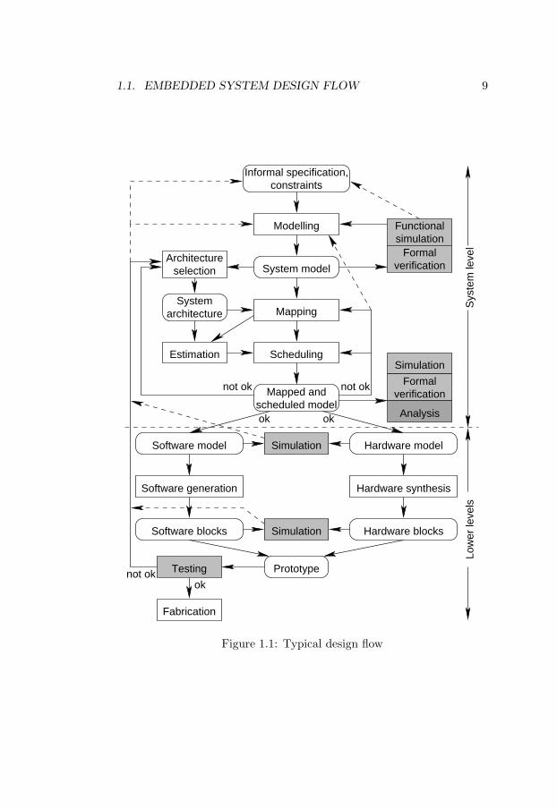
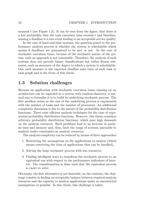
Designing such systems implies the deployment of different tech-niques with roots in system engineering, software engineering, com-puter architectures, specification languages, formal methods, real-timescheduling, simulation, programming languages, compilation, hardwaresynthesis, etc. Considering the huge complexity of such a design task,there is an urgent need for automatic tools for design, estimation andsynthesis in order to support and guide the designer. A rigorous, disci-plined and systematic approach to real-time embedded system design isthe only way the designer can cope with the complexity of current andfuture designs in the context of high time-to-market pressure. Such adesign flow is depicted in Figure 1.1 [Ele02].
The design process starts from a less formal specification togetherwith a set of constraints. This initial informal specification is then cap-tured as a more rigorous model formulated in one or possibly severalmodelling languages [JMEP00]. During the system level design space ex-ploration phase, different architecture, mapping and scheduling alterna-tives are assessed in order to meet the design requirements and possibly
1.1. EMBEDDED SYSTEM DESIGN FLOW 9
Informal specification,constraints
Modelling
System model
Mapping
Scheduling
Mapped andscheduled model
Estimation
Systemarchitecture
Architectureselection
Prototype
Hardware model
Hardware synthesis
Hardware blocks
Software model
Software generation
Software blocks
Fabrication
Simulation
Formalverification
Analysis
not oknot ok
okok
ok
Sys
tem
leve
lLo
wer
leve
ls
Formalverification
Functionalsimulation
Simulation
Simulation
Testingnot ok
Figure 1.1: Typical design flow
10 CHAPTER 1. INTRODUCTION
optimise certain indicators. The shaded blocks in the figure denote theactivities providing feedback concerning design fitness or performance tothe designer. The existence of accurate, fast and flexible automatic toolsfor performance estimation in every design phase is of capital importancefor cutting down design process iterations, time and implicitly cost.
Performance estimation tools can be classified in simulation and anal-ysis tools. Simulation tools are flexible, but there is always the dangerthat unwanted and extremely rare glitches in behaviour, possibly bring-ing the system to undesired states, are never observed. The probabilityof not observing such an existing behaviour can be decreased at the ex-pense of increasing the simulation time. Analysis tools are more precise,but they usually rely on a mathematical formalisation which is some-times difficult to come up with or to understand by the designer. Afurther drawback of analysis tools is their often prohibitive running timedue to the analysis complexity. A tool that trades, in a designer con-trolled way, analysis complexity (in terms of analysis time and memory,for example) with analysis accuracy or the degree of insight that it pro-vides, could be a viable solution to the performance estimation problem.Such an approach is the topic of this thesis.
The focus of this thesis is on the analytic performance estimationof soft real-time systems. Given an architecture, a mapping, a taskscheduling alternative, and the set of task execution time probabilitydistribution functions, such an analysis (the dark shaded box in Fig-ure 1.1) would provide important and fairly accurate results useful forguiding the designer through the design space.
1.2 Stochastic task execution times
Historically, real-time system research emerged from the need to under-stand, design, predict, and analyse safety critical applications such asplant control and aircraft control, to name a few. Therefore, the com-munity focused on hard real-time systems, where the only way to ensurethat no real-time requirement is broken was to make conservative as-sumptions about the systems. In hard real-time system analysis, eachtask instantiation is assumed to run for a worst case time interval, calledthe worst case execution time (WCET) of the task.
This approach is sometimes the only one applicable for the classof safety critical embedded systems. However, for a large class of softreal-time systems this approach leads to significant underutilisation ofcomputation resources, missing the opportunity to create much cheaperproducts with low or no perceived service quality reduction. For ex-

1.2. STOCHASTIC TASK EXECUTION TIMES 11
t WCET
prob
abili
ty d
ensi
ty
computation time
Figure 1.2: Execution time probability density function
ample, multimedia applications like JPEG and MPEG encoding, soundencoding, etc. exhibit this property.
The execution time of a task depends on application dependent, plat-form dependent, and environment dependent factors. The amount ofinput data to be processed in each task instantiation as well as its type(pattern, configuration) are application dependent factors. The type ofprocessing unit that executes a task is a platform dependent factor in-fluencing the task execution time. If the time needed for communicationwith the environment (database lookups, for example) is to be consideredas a part of the task execution time, then network load is an example ofan environmental factor influencing the task execution time.
Input data amount and type may vary, as for example is the case fordifferently coded MPEG frames. Platform dependent characteristics,like cache memory behaviour, pipeline stalls, write buffer queues, mayalso introduce a variation in the task execution time. Thus, obviously,all of the enumerated factors influencing the task execution time mayvary. Therefore, a model considering variable execution time would bemore realistic as the one considering fixed, worst case execution times. Inthe most general model, task execution times with arbitrary probabilitydistribution functions are considered. Obviously, the fixed task executiontime model is a particular case of such a stochastic one.
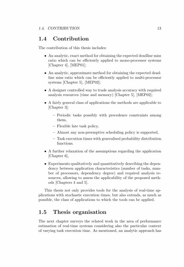
Figure 1.2 shows the execution time probability density of such atask. An approach based on a worst case execution time model wouldimplement the task on an expensive system which guarantees the im-posed deadline for the worst case situation. This situation, however, willoccur with a very small probability. If the nature of the application issuch that a certain percentage of deadline misses is affordable, a cheapersystem, which still fulfils the imposed quality of service, can be designed.For example, such a cheaper a system would be one that would guaran-tee the deadlines if the execution time of the task did not exceed a time
12 CHAPTER 1. INTRODUCTION
moment t (see Figure 1.2). It can be seen from the figure, that there isa low probability that the task execution time exceeds t and therefore,missing a deadline is a rare event leading to an acceptable service quality.
In the case of hard real-time systems, the question posed to the per-formance analysis process is whether the system is schedulable whichmeans if deadlines are guaranteed to be met or not. In the case ofstochastic execution times, because of the stochastic nature of the sys-tem, such an approach is not reasonable. Therefore, the analysis of suchsystems does not provide binary classifications but rather fitness esti-mates, such as measures of the degree to which a system is schedulable.One such measure is the expected deadline miss ratio of each task ortask graph and is the focus of this thesis.
1.3 Solution challenges
Because an application with stochastic execution times running on anarchitecture can be regarded as a system with random character, a nat-ural way to formalise it is to build its underlying stochastic process. Thefirst problem arises as the size of the underlying process is exponentialwith the number of tasks and the number of processors. An additionalcomplexity dimension is due to the nature of the probability distributionfunctions. There exist efficient analysis techniques for the case of expo-nential probability distribution functions. However, this thesis considersarbitrary probability distribution functions, which pose high demandson the analysis resources. Both problems lead to an increase in analy-sis time and memory and, thus, limit the range of systems amenable toanalysis under constraints on analysis resources.
The analysis complexity can be reduced by means of three approaches:
1. Restricting the assumptions on the applications to analyse (whichmeans restricting the class of applications that can be handled),
2. Solving the large stochastic process with less resources,
3. Finding intelligent ways to transform the stochastic process to anequivalent one with respect to the performance indicators of inter-est. The transformation is done such that the equivalent processis easier to solve.
Obviously, the first alternative is not desirable, on the contrary, the chal-lenge consists in finding an acceptable balance between required analysisresources and the capacity to analyse applications under as unrestrictedassumptions as possible. In this thesis, this challenge is taken.
1.4. CONTRIBUTION 13
1.4 Contribution
The contribution of this thesis includes:
• An analytic, exact method for obtaining the expected deadline missratio which can be efficiently applied to mono-processor systems[Chapter 4], [MEP01];
• An analytic, approximate method for obtaining the expected dead-line miss ratio which can be efficiently applied to multi-processorsystems [Chapter 5], [MEP02];
• A designer controlled way to trade analysis accuracy with requiredanalysis resources (time and memory) [Chapter 5], [MEP02];
• A fairly general class of applications the methods are applicable to[Chapter 3]:
– Periodic tasks possibly with precedence constraints amongthem,
– Flexible late task policy,
– Almost any non-preemptive scheduling policy is supported,
– Task execution times with generalised probability distributionfunctions.
• A further relaxation of the assumptions regarding the application[Chapter 6],
• Experiments qualitatively and quantitatively describing the depen-dency between application characteristics (number of tasks, num-ber of processors, dependency degree) and required analysis re-sources, allowing to assess the applicability of the proposed meth-ods [Chapters 4 and 5].
This thesis not only provides tools for the analysis of real-time ap-plications with stochastic execution times, but also extends, as much aspossible, the class of applications to which the tools can be applied.
1.5 Thesis organisation
The next chapter surveys the related work in the area of performanceestimation of real-time systems considering also the particular contextof varying task execution time. As mentioned, an analytic approach has
14 CHAPTER 1. INTRODUCTION
to rely on a mathematical formalisation of the problem. The notationused throughout the thesis and the problem formulation are introducedin Chapter 3. The first approach to solve the problem, efficiently appli-cable to mono-processor systems, is detailed in Chapter 4. The secondapproach, applicable to multiprocessor systems, is presented in Chap-ter 5. Chapter 6 discusses relaxations on the initial assumptions as wellas extensions of the results and their impact on the analysis complex-ity. Finally, Chapter 7 draws the conclusions and presents directions offuture work.
Chapter 2
Background and RelatedWork
This chapter is structured in three sections. The first provides a back-ground in schedulability analysis. The second section surveys some ofthe related work in the area of schedulability analysis of real-time sys-tems with stochastic task execution times. The third section informallypresents some of the concepts in probability theory and in the theory ofstochastic processes to be used in the following chapters.
The earliest results in real-time scheduling and schedulability analysishave been obtained under restrictive assumptions about the task set andthe underlying architecture. Thus, in the early literature, task sets withthe following properties have been considered, referred in this thesis asthe restricted assumptions: The task set is composed of a fixed number ofindependent tasks mapped on a single processor, the tasks are periodicallyreleased, each with a fixed period, the deadlines equal the periods, and thetask execution times are fixed.
Later work was done under more relaxed assumptions. This surveyof related work is limited to research considering assumption relaxationsalong some of the following dimensions, of interest in the context of thisthesis:
• Multi-processor systems
• Data dependency relationships among the tasks
• Stochastic task execution times
• Deadlines less than or equal to the periods
15
16 CHAPTER 2. BACKGROUND AND RELATED WORK
• Late task policy
Note also that applications with sporadic or aperiodic tasks, or taskswith resource constraints, or applications with dynamic mapping of tasksto processors have not been considered in this overview.
2.1 Schedulability analysis of hard real-timesystems
2.1.1 Mono-processor systems
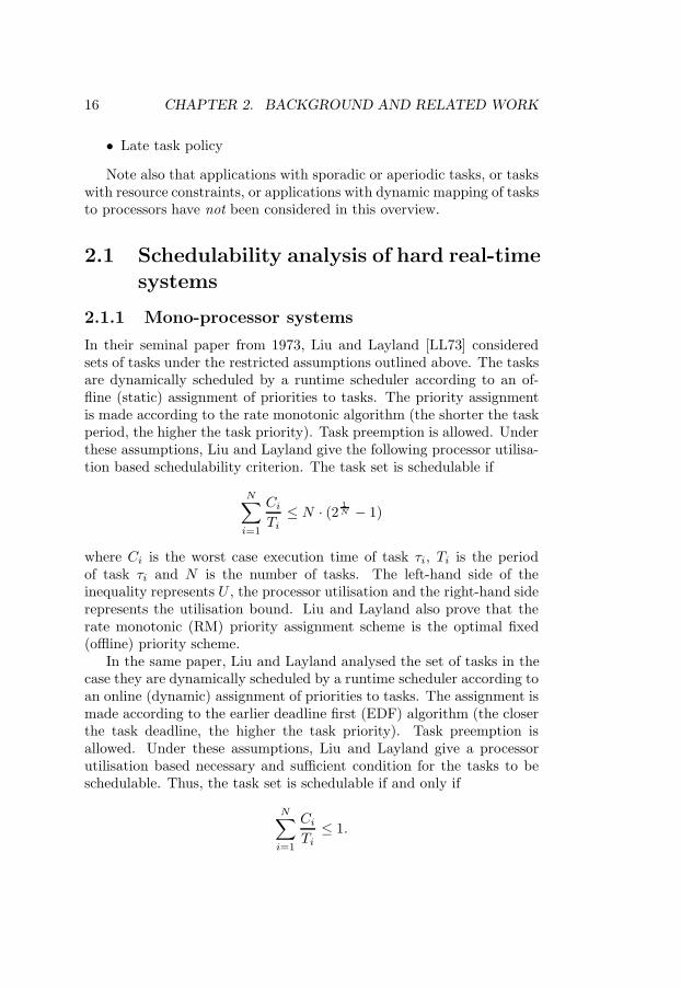
In their seminal paper from 1973, Liu and Layland [LL73] consideredsets of tasks under the restricted assumptions outlined above. The tasksare dynamically scheduled by a runtime scheduler according to an of-fline (static) assignment of priorities to tasks. The priority assignmentis made according to the rate monotonic algorithm (the shorter the taskperiod, the higher the task priority). Task preemption is allowed. Underthese assumptions, Liu and Layland give the following processor utilisa-tion based schedulability criterion. The task set is schedulable if
N∑i=1
Ci
Ti≤ N · (2 1
N − 1)
where Ci is the worst case execution time of task τi, Ti is the periodof task τi and N is the number of tasks. The left-hand side of theinequality represents U , the processor utilisation and the right-hand siderepresents the utilisation bound. Liu and Layland also prove that therate monotonic (RM) priority assignment scheme is the optimal fixed(offline) priority scheme.
In the same paper, Liu and Layland analysed the set of tasks in thecase they are dynamically scheduled by a runtime scheduler according toan online (dynamic) assignment of priorities to tasks. The assignment ismade according to the earlier deadline first (EDF) algorithm (the closerthe task deadline, the higher the task priority). Task preemption isallowed. Under these assumptions, Liu and Layland give a processorutilisation based necessary and sufficient condition for the tasks to beschedulable. Thus, the task set is schedulable if and only if
N∑i=1
Ci
Ti≤ 1.
2.1. SCHEDULABILITY ANALYSIS 17
They also prove that EDF is the optimal dynamic priority assignmentalgorithm. Optimality, in the context of RM and EDF scheduling, meansthat if there exists an offline [online] task priority assignment methodunder which the tasks are schedulable, then they are also schedulableunder the RM [EDF] assignment method.
Recently, E. Bini et al. [BBB01] improved the bound given by Liu andLayland for the rate monotonic algorithm. Thus, a task set is schedulableunder the same assumptions if
N∏i=1
(Ci
Ti+ 1)
≤ 2.
Checking of the schedulability conditions presented above has complexityO(N).
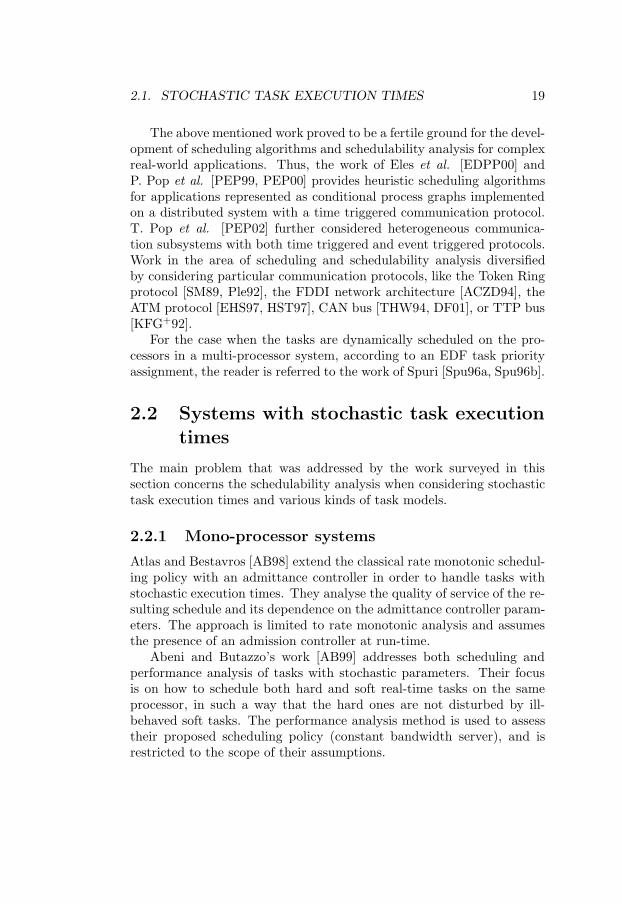
A necessary and sufficient condition for schedulability under the re-stricted assumptions and a fixed priority preemptive scheduling of taskshas been given by Lehoczky et al. [LSD89]. A task τi is schedulable ifand only if there exists a time moment t ∈ [0, Ti] such that
t ≥N∑
j∈HPi
Cj ·⌈
t
Ti
⌉,
where HPi = j : prior(τj) ≥ prior(τi). They have also shown thatit is sufficient to check the schedulability condition only at the releasetimes of higher priority tasks. Still, the algorithm is pseudo-polynomial.
If the task deadlines are less than the corresponding periods, a dead-line monotonic task priority assignment algorithm was proposed by Le-ung and Whitehead [LW82]. Such a scheme assigns a higher priorityto the task with the shorter relative deadline. Leung and Whiteheadalso proved that this algorithm is the optimal fixed priority assignmentalgorithm under the considered assumptions and gave a schedulabilitycriterion. Audsley et al. [ABD+91] extended the work of Joseph andPandya [JP86] about response time analysis and derived a necessaryand sufficient condition for schedulability under the deadline monotonicapproach. Manabe and Aoyagi [MA95] gave similar schedulability con-ditions reducing the number of time moments that have to be evaluated,but their schedulability analysis algorithm is pseudo-polynomial as well.
In the case of deadlines less than periods and dynamic priority as-signment according to an EDF policy, a necessary and sufficient schedu-lability condition has been given by Baruah et al. [BRH90]. Their testis pseudo-polynomial.
18 CHAPTER 2. BACKGROUND AND RELATED WORK
Less work has been carried out when considering task sets with prece-dence relationships among tasks. Audsley et al. [ABRW93] provideschedulability criteria under the assumption that the tasks are dynam-ically scheduled according to an offline (static) assignment of task pri-orities. The precedence relationships are implicitly enforced by care-fully choosing the task periods, offsets and deadlines but this makes theanalysis pessimistic. Gonzalez Harbour et al. [GKL91, GKL94] con-sider certain types of precedence relationships among tasks and provideschedulability criteria for these situations. Sun et al. [SGL97] addi-tionally extend the approach by considering fixed release times for thetasks.
Blazewicz [Bla76] showed how to modify the task deadlines underthe assumptions of precedence relationships among tasks that are dy-namically scheduled according to an online assignment of task prioritiesbased on EDF. He has also shown that the resulting EDF∗ algorithm isoptimal. Sufficient conditions for schedulability under the mentioned as-sumptions are given by Chetto et al. [CSB90] while Spuri and Stankovic[SS94] consider also shared resources.
2.1.2 Multi-processor systems
Most problems related to hard real-time scheduling on multi-processorsystems under non-trivial assumptions have been proven to be NP-complete [GJ75, Ull75, GJ79, SSDB94].
The work of Sun and Liu [SL95] addresses multi-processor real-timesystems where the application exhibits a particular form of precedencerelationships among tasks, namely the periodic job-shop model. Sunand Liu have provided analytic bounds for the task response time undersuch assumptions. The results, plus heuristics on how to assign fixedpriorities to tasks under the periodic job-shop model, are summarised inSun’s thesis [Sun97].
Audsley [Aud91] and Audsley et al. [ABR+93] provide a schedulabil-ity analysis method based on the task response time analysis where thetasks are allowed to be released at arbitrary time moments. Includingthese jitters in the schedulability analysis provides for the analysis ofapplications with precedence relationships among tasks. Tindell [Tin94]and Tindell and Clark [TC94] extend this schedulability analysis by ap-plying it to multi-processor systems coupled by time triggered communi-cation links. Later on, Palencia Gutierrez and Gonzalez Harbour [PG98]improved on Tindell’s work by allowing dynamic task offsets, obtainingtighter bounds for task response times.
2.1. STOCHASTIC TASK EXECUTION TIMES 19
The above mentioned work proved to be a fertile ground for the devel-opment of scheduling algorithms and schedulability analysis for complexreal-world applications. Thus, the work of Eles et al. [EDPP00] andP. Pop et al. [PEP99, PEP00] provides heuristic scheduling algorithmsfor applications represented as conditional process graphs implementedon a distributed system with a time triggered communication protocol.T. Pop et al. [PEP02] further considered heterogeneous communica-tion subsystems with both time triggered and event triggered protocols.Work in the area of scheduling and schedulability analysis diversifiedby considering particular communication protocols, like the Token Ringprotocol [SM89, Ple92], the FDDI network architecture [ACZD94], theATM protocol [EHS97, HST97], CAN bus [THW94, DF01], or TTP bus[KFG+92].
For the case when the tasks are dynamically scheduled on the pro-cessors in a multi-processor system, according to an EDF task priorityassignment, the reader is referred to the work of Spuri [Spu96a, Spu96b].
2.2 Systems with stochastic task execution
times
The main problem that was addressed by the work surveyed in thissection concerns the schedulability analysis when considering stochastictask execution times and various kinds of task models.
2.2.1 Mono-processor systems
Atlas and Bestavros [AB98] extend the classical rate monotonic schedul-ing policy with an admittance controller in order to handle tasks withstochastic execution times. They analyse the quality of service of the re-sulting schedule and its dependence on the admittance controller param-eters. The approach is limited to rate monotonic analysis and assumesthe presence of an admission controller at run-time.
Abeni and Butazzo’s work [AB99] addresses both scheduling andperformance analysis of tasks with stochastic parameters. Their focusis on how to schedule both hard and soft real-time tasks on the sameprocessor, in such a way that the hard ones are not disturbed by ill-behaved soft tasks. The performance analysis method is used to assesstheir proposed scheduling policy (constant bandwidth server), and isrestricted to the scope of their assumptions.
20 CHAPTER 2. BACKGROUND AND RELATED WORK
Tia et al. [TDS+95] assume a task model composed of independenttasks. Two methods for performance analysis are given. One of themis just an estimate and is demonstrated to be overly optimistic. In thesecond method, a soft task is transformed into a deterministic task anda sporadic one. The latter is executed only when the former exceeds thepromised execution time. The sporadic tasks are handled by a serverpolicy. The analysis is carried out on this model.
Zhou et al. [ZHS99] and Hu et al. [HZS01] root their work in Tia’s.However, they do not intend to give per-task guarantees, but characterisethe fitness of the entire task set. Because they consider all possiblecombinations of execution times of all requests up to a time moment,the analysis can be applied only to small task sets due to complexityreasons.
De Veciana et al. [dJG00] address a different type of problem. Havinga task graph and an imposed deadline, they determine the path thathas the highest probability to violate the deadline. The problem is thenreduced to a non-linear optimisation problem by using an approximationof the convolution of the probability densities.
Lehoczky [Leh96] models the task set as a Markovian process. Theadvantage of such an approach is that it is applicable to arbitrary schedul-ing policies. The process state space is the vector of lead-times (timeleft until the deadline). As this space is potentially infinite, Lehoczkyanalyses it in heavy traffic conditions, when the system provides a sim-ple solution. The main limitations of this approach are the non-realisticassumptions about task inter-arrival and execution times.
Kalavade and Moghe [KM98] consider task graphs where the task ex-ecution times are arbitrarily distributed over discrete sets. Their analysisis based on Markovian stochastic processes too. Each state in the pro-cess is characterised by the executed time and lead-time. The analysisis performed by solving a system of linear equations. Because the exe-cution time is allowed to take only a finite (most likely small) numberof values, such a set of equations is small.
2.2.2 Multi-processor systems
Burman has pioneered the ”heavy traffic” school of thought in the areaof queueing [Bur79]. Lehoczky later applied and extended it in the areaof real-time systems [Leh96, Leh97]. The theory was further extendedby Harrison and Nguyen [HN93], Williams [Wil98] and others [PKH01,DLS01, DW93]. The application is modelled as a multi-class queueingnetwork. This network behaves as a reflected Brownian motion with
2.2. ELEMENTS OF PROBABILITY THEORY 21
drift under heavy traffic conditions, i.e. when the processor utilisationsapproach 1, and therefore it has a simple solution.
Other researchers, such as Kleinberg et al. [KRT00] and Goel and In-dyk [GI99], apply approximate solutions to problems exhibiting stochas-tic behaviour but in the context of load balancing, bin packing and knap-sack problems. Moreover, the probability distributions they consider arelimited to a few very particular cases.
Kim and Shin [KS96] modelled the application as a queueing network,but restricted the task execution times to exponentially distributed ones,which reduces the complexity of the analysis. The tasks were consideredto be scheduled according to a particular policy, namely FIFO. Theunderlying mathematical model is then the appealing continuous timeMarkov chain (CTMC).
Our work is mostly related to the ones of Zhou et al. [ZHS99] and Huet al. [HZS01], and Kalavade and Moghe [KM98]. Mostly, it differs byconsidering less restricted application classes. As opposed to Kalavadeand Moghe’s work, we consider continuous ETPDFs. Also, we accepta much larger class of scheduling policies than the fixed priority onesconsidered by Zhou and Hu. Moreover, our original way of concurrentlyconstructing and analysing the underlying process, while keeping onlythe needed stochastic process states in memory, allows us to considerlarger applications.
As far as we are aware, the heavy traffic theory fails yet to smoothlyapply to real-time systems. Not only that there are cases when such areflected Brownian motion with drift limit does not exist, as shown byDai [DW93], but also the heavy traffic phenomenon is observed only forprocessor loads close to 1, leading to very long (infinite) queues of readytasks and implicitly to systems with very large latency. This aspectmakes the heavy traffic phenomenon undesirable in real-time systems.
In the context of multi-processor systems, our work significantly ex-tends the one by Kim and Shin [KS96]. Thus, we consider arbitraryETPDFs (Kim and Shin consider exponential ones) and we address amuch larger class of scheduling policies (as opposed to FCFS consideredby them).
2.3 Elements of probability theory and
stochastic processes
This section informally introduces some of the probability theory con-cepts needed in the following chapters. For a more formal treatment of

22 CHAPTER 2. BACKGROUND AND RELATED WORK
the subject, the reader is referred to Appendix B and to J. L. Doob’s“Measure Theory” [Doo94].
Consider a set of events. An event may be the arrival or the comple-tion of a task, as well as a whole sequence of actions, as for example “taskτ starts at moment t1, and it is discarded at time moment t2”. A randomvariable is a mapping that associates a real number to an event. The dis-tribution of a random variable X is a real function F , F (x) = P(X ≤ x).F (x) indicates what is the probability of the events that are mapped toreals less than or equal to x. Obviously, F is monotone increasing and itslimit limx→∞ = 1. Its first derivative f(x) = dF (x)
dx is the probability den-sity of the random variable. If the distribution function F is continuous,the random variable it corresponds to is said to be continuous.
If P(X ≤ t + u|X > t) = P(X ≤ u) then X (or its distribution) ismemoryless. For example, if X is a finishing time of a task τ and X ismemoryless, then the probability that τ completes its execution before atime moment t2, knowing that by time t1 it has not yet finished, is equalto the probability of τ finishing in t2 − t1 time units. Hence, if the taskexecution time is distributed according to a memoryless distribution, theprobability of τ finishing before t time units is independent of how muchit has run already.
If the distribution of a random variable X is F of the form F (t) = 1−e−λt, then X is exponentially distributed. The exponential distributionis the only continuous memoryless distribution.
A family of random variables Xt : t ∈ I1 is a stochastic process.The set S of values of Xt form the state space of the stochastic process. IfI is a discrete set, then the stochastic process is a discrete time stochasticprocess. Otherwise it is a continuous time stochastic process. If S is adiscrete set, the stochastic process is a discrete state process or a chain.The interval between two consecutive state transitions in a stochasticprocess denotes the state holding interval.
Consider a continuous time stochastic process Xt : t ≥ 0 witharbitrarily distributed state holding time probabilities and consider Ito be the ordered set (t1, t2, . . . , tk, . . . ) of time moments when a statechange occurs in the stochastic process. The discrete time stochasticprocess Xn : tn ∈ I is the embedded discrete time process of Xt : t ≥0.
We are interested in the steady state probability of a given state,i.e. the probability of the stochastic process being in a given state inthe long run. This indicates also the percentage of time the stochasticprocess spends in that particular state. The usefulness of this value
1Denoted also as Xtt∈I
2.3. ELEMENTS OF PROBABILITY THEORY 23
is highlighted in the following example. Consider a stochastic processXt where Xt = i indicates that the task τi is currently running. State0 is the idle state, when no task is running. Let us assume that weare interested in the expected rate of a transition from state 0 to statei, that is, how many times per second the task τi is activated after aperiod of idleness. If we know the average rate of the transition fromidleness (state 0) to τi running (state i) given that the processor is idle,the desired value is computed by multiplying this rate by the percentageof time the processor is indeed idle. This percentage is given by thesteady state probability of the state 0.
Consider a stochastic process Xt : t ≥ 0. If the probability thatthe system is in a given state j at some time t + u in the future, giventhat it is in state j at the present time t and that its past states Xs,s < t, are known, is independent of these past states Xs (P(Xt+u =j|Xt = i, Xs, 0 ≤ s < t, u > 0) = P(Xt+u = j|Xt = i, u > 0)), thenthe stochastic process exhibits the Markov property and it is a Markovprocess. Continuous time Markov chains are abbreviated CTMC anddiscrete time ones are abbreviated DTMC. If the embedded discrete timeprocess of a continuous time process Xtt≥0 is a discrete time Markovprocess, then Xtt≥0 is a semi-Markov process.
To exemplify, consider a stochastic process where Xt denotes the taskrunning on a processor at time t. The stochastic process is Markovianif the probability of task τj running in the future does not depend onwhich tasks have run in the past knowing that τi is running now.
It can be shown that a continuous time Markov process must haveexponentially distributed state holding interval length probabilities. Ifwe construct a stochastic process where Xt denotes the running taskat time moment t, then a state transition occurs when a new task isscheduled on the processor. In this case, the state holding times corre-spond to the task execution times. Therefore, such a process cannot beMarkovian if the task execution time probabilities are not exponentiallydistributed.
The steady state probability vector can relatively simply be com-puted by solving a linear system of equations in the case of Markovprocesses (both discrete and continuous ones). This property, as well asthe fact that Markov processes are easier to conceptualise, makes them apowerful instrument in the analysis of systems with stochastic behaviour.

24 CHAPTER 2. BACKGROUND AND RELATED WORK
Chapter 3
Problem Formulation
In this chapter, we introduce the notations used throughout the thesisand give an exact formulation of the problem. Some relaxations of theassumptions introduced in this chapter and extensions of the problemformulation will be further discussed in Chapter 6.
3.1 Notation
3.1.1 System architecture
Let PE = PE1, PE2, . . . , PEp be a set of p processing elements.These can be programmable processors of any kind (general purpose,controllers, DSPs, ASIPs, etc.). Let B = B1, B2, . . . , Bl be a set of lbuses connecting various processing elements of PE.
Unless explicitly stated, the two types of hardware resources, pro-cessing elements and buses, will not be treated differently in the scopeof this thesis, and therefore they will be denoted with the general termof processors. Let M = p + l and P = PE ∪ B = P1, P2, . . . , PM bethe set of processors.
3.1.2 Functionality
Let PT = t1, t2, . . . , tn be a set of n processing tasks. Let CT =χ1, χ2, . . . , χm be a set of m communication tasks.
Unless explicitly stated, the processing and the communication taskswill not be differently treated in the scope of this thesis, and thereforethey will be denoted with the general term of tasks. Let N = n+m andT = PT ∪ CT = τ1, τ2, . . . , τN denote the set of tasks.
25

26 CHAPTER 3. PROBLEM FORMULATION
Let G = G1, G2, . . . , Gh denote h task graphs. A task graph Gi =(Vi, Ei ⊂ Vi ×Vi) is a directed acyclic graph (DAG) whose set of verticesVi is a non-empty subset of the set of tasks T . The sets Vi, 1 ≤ i ≤ h,form a partition of T . There exists a directed edge (τi, τj) ∈ Ei if andonly if the task τj is data dependent on the task τi. This data dependencyimposes that the task τj is executed only after the task τi has completedexecution.
Let Gi = (Vi, Ei) and τk ∈ Vi. Then let τk = τj : (τj , τk) ∈ Eidenote the set of predecessor tasks of the task τi. Similarly, let τ
k =τj : (τk, τj) ∈ Ei denote the set of successor tasks of the task τk. Ifτk = ∅ then task τk is a root. If τ
k = ∅ then task τk is a leaf.Obviously, some consistency rules have to apply. Thus, a commu-
nication task has to have exactly one predecessor task and exactly onesuccessor task, and these tasks have to be processing tasks.
Let Π = π1, π2, . . . , πh denote the set of task graph periods, or taskgraph inter-arrival times. Each πi time units, a new instantiation oftask graph Gi demands execution. In the special case of mono-processorsystems, the concept of period will be applied to individual tasks, withcertain restrictions (see Section 6.1).
The real-time requirements are expressed in terms of relative dead-lines. Let ∆ = δ1, δ2, . . . , δh denote the set of task graph deadlines. δi
is the deadline for task graph Gi = (Vi, Ei). If there is a task τ ∈ Vi
that has not completed its execution at the moment of the deadline δi,then the entire graph Gi missed its deadline.
The deadlines are supposed to coincide with the arrival of the nextgraph instantiation (δi = πi). This restriction will later be relaxed inthe case of mono-processor systems [Section 6.2].
If Di(t) denotes the number of missed deadlines of graph Gi over atime span t and Ai(t) denotes the number of instantiations of graph Gi
over the same time span, then mi = limt→∞Di(t)Ai(t)
denotes the expecteddeadline miss ratio of task graph Gi.
3.1.3 Mapping
Let MapP : PT → PE be a surjective function that maps processingtasks on the processing elements. MapP (ti) = Pj indicates that process-ing task ti is executed on the processing element Pj . Let MapC : CT →B be a surjective function that maps communication tasks on buses.MapC(χi) = Bj indicates that the communication task χi is performedon the bus Bj . For notation simplicity, Map : T → P is defined, whereMap(τi) = MapP (τi) if τi ∈ PT and Map(τi) = MapC(τi) if τi ∈ CT .
3.1. NOTATION 27
3.1.4 Execution times
Let Exi denote an execution time of an instantiation of the task ti. LetET = ε1, ε2, . . . , εN denote a set of N execution time probability den-sity functions (ETPDFs). εi is the probability density of the executiontime (or communication time) of task (communication) τi on the proces-sor (bus) Map(τi). The execution times are assumed to be statisticallyindependent.
3.1.5 Late tasks policy
If a task misses its deadline, the real-time operating system takes adecision based on a designer-supplied late task policy. Let Bounds =b1, b2, . . . , bh be a set of h integers greater than 0. The late task policyspecifies that at most bi instantiations of the task graph Gi are allowed inthe system at any time. If an instantiation of graph Gi demands execu-tion when bi instantiations already exist in the system, the instantiationwith the earliest arrival time is discarded (eliminated) from the system.An alternative to this late task policy will be discussed in Section 6.4
3.1.6 Scheduling
In the common case of more than one task mapped on the same proces-sor, the designer has to decide on a scheduling policy. Such a schedulingpolicy has to be able to unambiguously determine the running task atany time on that processor.
Let an event denote a task arrival, departure or discarding. In orderto be acceptable in the context described in this thesis, a schedulingpolicy is assumed to preserve the sorting of tasks according to their ex-ecution priority between consecutive events (the priorities are allowedto change in time, but the sorting of tasks according to their prioritiesis allowed to change only at event times). All practically used prior-ity based scheduling policies, both with static priority assignment (ratemonotonic, deadline monotonic) and with dynamic assignment (EDF,LLF) fulfill this requirement. The scheduling policy is restricted to non-preemptive scheduling.
28 CHAPTER 3. PROBLEM FORMULATION
3.2 Problem formulation
This section gives the problem formulation.
3.2.1 Input
The following data is given as an input to the analysis procedure:
• The set of task graphs G,
• The set of processors P ,
• The mapping Map,
• The set of task graph periods Π,
• The set of task graph deadlines ∆,
• The set of execution time probability density functions ET ,
• The late task policy Bounds, and
• The scheduling policy.
3.2.2 Output
The result of the analysis is the set Missed = m1, m2, . . . , mh ofexpected deadline miss ratios for each task graph.
The problem formulation is extended in Section 6.3 by including theexpected deadline miss ratios for each task in the results.
3.3 Example
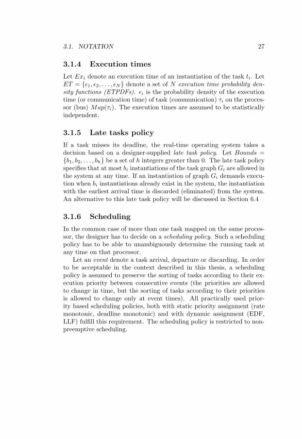
Figure 3.1 depicts a hardware architecture consisting of the set PE ofthree (p = 3) processing elements PE1 (white), PE2 (dashed), and PE3
(solid gray) and the set B of two (l = 2) communication buses B1 (thick
PE1 PE3PE2
B2
B1
Figure 3.1: System architecture

3.3. EXAMPLE 29
χ1
χ2
χ3
χ4
1 2
3
4 5
7 8
6
9
10
t t t
tt
t t t
t t
Figure 3.2: Application graphs
hollow line) and B2 (thin line). The total number of processors M =p + l = 5 in this case.
Figure 3.2 depicts an application that runs on the architecture givenabove. The application consists of the set G of three (h = 3) taskgraphs G1, G2, and G3. The set PT of processing tasks consists of ten(n = 10) processing tasks t1, t2, . . . , t10. The set of communication tasksCT consists of four (m = 4) communication tasks χ1, χ2, . . . , χ4. Thetotal number of tasks N = n + m = 14 in this case. According to theaffiliation to task graphs, the set T of tasks is partitioned as follows.T = V1 ∪ V2 ∪ V3, V1 = t1, t2, . . . , t5, χ1, χ2, V2 = t6, t7, t8, t9, χ3, χ4,V3 = t10. The predecessor set of t3, for instance, is t3 = t1, χ1and its successor set is t3 = t4, χ2. The edge (t1, t3) indicates, forexample, that an instantiation of the task t3 may run only after aninstantiation of the task t1 belonging to the same task graph instantiationhas successfully completed its execution. The set of task graph periods Πis 6, 4, 3. This means that every π1 = 6 time units a new instantiationof task graph G1 will demand execution. Each of the three task graphshas an associated deadline, δ1, δ2 and δ3, and these deadlines are assumedto be equal to the task graph periods π1, π2 and π3 respectively.
The tasks t1, t3, t4, and t9 (depicted as white circles) are mapped onthe processing element PE1, the tasks t2, t6, and t7 (depicted as dashedcircles) are mapped on the processing element PE2, and the tasks t5, t8,and t10 (depicted as gray circles) are mapped on the processing elementPE3. The communication between t2 and t3 (the communication taskχ1) is mapped on the point-to-point link B2 whereas the other threecommunication tasks share the bus B1.
30 CHAPTER 3. PROBLEM FORMULATION
execution timeexecution time
prob
abili
ty d
ensi
ty
prob
abili
ty d
ensi
ty
Figure 3.3: Execution time probability density functions example
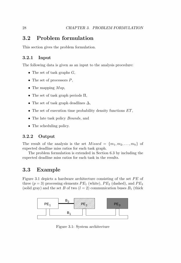
Figure 3.3 depicts a couple of possible execution/communication timeprobability density functions (ETPDFs). There is no restriction on thesupported type of probability density functions.
The late task policy is specified by the set of integers Bounds =1, 1, 2. It indicates that, as soon as one instantiation of G1 or G2 is late,that particular instantiation is discarded from the system (1 indicatesthat only one instantiation of the graph is allowed in the system at thesame time). However, one instantiation of the graph G3 is tolerated tobe late (there may be two simultaneously active instantiations of G3).
A possible scheduling policy could be fixed priority scheduling, forexample. As the task priorities do not change, this policy obviously sat-isfies the restriction that the sorting of tasks according to their prioritiesmust be unique between consecutive events.
A Gantt diagram illustrating a possible task execution over a spanof 20 time units is depicted in Figure 3.4. The different task graphs aredepicted in different shades in this figure. Note the two simultaneousinstantiations of t10 in the time span 9–9.375. Note also the discardingof the task graph G1 happening at the time moment 12 due to thelateness of task t5. It follows that the deadline miss ratio of G1 over theinterval [0, 18) is 1/3 (one instantiations out of three missed its deadline).The deadline miss ratio of G3 over the same interval is 1/6, becausethe instantiation that arrived at time moment 6 missed its deadline.When analysing this system, the expected deadline miss ratio of G1 (theratio of the number instantiations that missed their deadline and thetotal number of instantiations over an infinite time interval) is 0.4. Theexpected deadline miss ratio of G3 is 0.08 and the one of G2 is 0.15.

3.3
.E
XA
MP
LE
31
0 1 2 3 4 5 6 7 8 9 10 11 12 13 14 15 16 17 18 19 20
0 1 2 3 4 5 6 7 8 9 10 11 12 13 14 15 16 17 18 19 20
0 1 2 3 4 5 6 7 8 9 10 11 12 13 14 15 16 17 18 19 20
0 1 2 3 4 5 6 7 8 9 10 11 12 13 14 15 16 17 18 19 20
0 1 2 3 4 5 6 7 8 9 10 11 12 13 14 15 16 17 18 19 20
t1 t1 t1 t1
t2 t2 t2t2
t3 t3 t3 t3t4 t4 t4
t5 t5 t5
t6 t6 t6 t6 t6 t6t7t7t7t7t7
t8 t8 t8 t8 t8t10 t10 t10 t10 t10 t10 t10
t9t9t9t9t9
χ1
χ2χ3 χ4 χ3 χ4
χ1
χ3 χ2 χ4
χ1
χ4χ3 χ2 χ3 χ4
χ1
PE1
PE2
PE3
B1
B2
Figure 3.4: Gantt diagram
32 CHAPTER 3. PROBLEM FORMULATION
Chapter 4
An Exact Solution forSchedulability Analysis:The Mono-processorCase
This chapter presents an exact approach for determining the expecteddeadline miss ratios of task graphs in the case of mono-processor sys-tems. First, it describes the stochastic process underlying the applica-tion, and shows how to construct such a stochastic process in order toobtain a semi-Markov process. Next, it introduces the concept of prioritymonotonicity intervals (PMIs) and shows how to significantly reduce theproblem complexity by making use of this concept. Then, the construc-tion of the stochastic process and its analysis are illustrated by meansof an example. Finally, a more concise formulation of the algorithm isgiven and experimental results are presented.
4.1 The underlying stochastic process
Let us consider the problem as defined in Section 3.2 and restrict it tomono-processor systems, i.e. P = PE = PE1; B = ∅; CT = ∅;Map(τi) = PE1, ∀τi ∈ T ; p = 1; l = 0; m = 0; and M = 1.
The goal of the analysis is to obtain the expected deadline miss ratiosof the task graphs. These can be derived from the behaviour of thesystem. The behaviour is defined as the evolution of the system through
33
34 CHAPTER 4. EXACT SOLUTION
a state space in time. A state of the system is given by the values of aset of variables that characterise the system. Such variables may be thecurrently running task, the set of ready tasks, the current time and thestart time of the current task, etc.
Due to the considered periodic task model, the task arrival timesare deterministically known. However, because of the stochastic taskexecution times, the completion times and implicitly the running taskat an arbitrary time instant or the state of the system at that instantcannot be deterministically predicted.
The mathematical abstraction best suited to describe and analysesuch a system with random character is the stochastic process.1 In thesequel, several alternatives for constructing the underlying stochasticprocess and its state space are illustrated and the most appropriate onefrom the analysis point of view is finally selected.
The following example is used in order to discuss the constructionof the stochastic process. The system consists of one processor and thefollowing application: G = (τ1, ∅), (τ2, ∅), Π = 3, 5, i.e. a setof two independent tasks with corresponding periods 3 and 5. The tasksare scheduled according to an EDF scheduling policy. For simplicity,in this example it is assumed that a late task is immediately discarded(b1 = b2 = 1). The application is observed over the time interval [0, 6].At time moment 0 both tasks are ready to run and task τ1 is activatedbecause it has the closest deadline. Consider the following four possibleexecution traces:
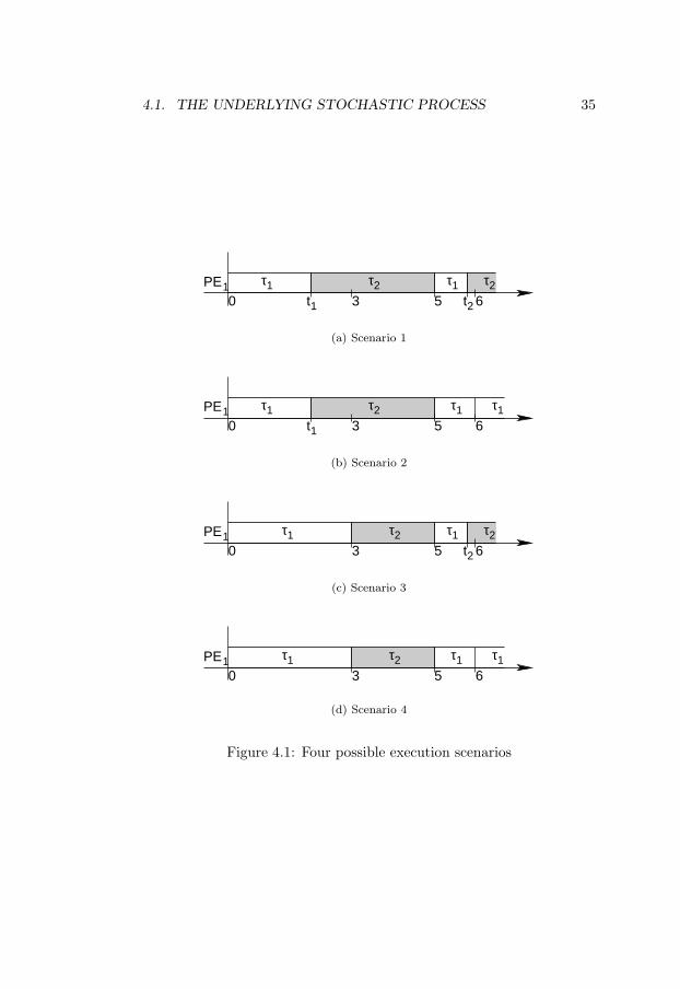
1. Task τ1 completes its execution at time moment t1 < 3. Task τ2
is then activated and, because it attempts to run longer than itsdeadline 5, it is discarded at time moment 5. The instance of taskτ1 that arrived at time moment 3 is activated and it completesits execution at time moment t2 < 6. At its completion time, theinstantiation of task τ2 that arrived at time moment 5 is activated.Figure 4.1(a) illustrates a Gantt diagram corresponding to thisscenario.
2. The system behaves exactly like in the previous case until timemoment 5. In this scenario, however, the second instantiation oftask τ1 attempts to run longer than its deadline 6 and it is discardedat 6. The new instance of task τ1 that arrived at time moment 6 isthen activated on the processor. This scenario corresponds to theGantt diagram in Figure 4.1(b).
1The mathematical concepts used in this thesis are informally introduced in Sec-tion 2.3, and more formally in Appendix B.
4.1. THE UNDERLYING STOCHASTIC PROCESS 35
PE1 τ1 τ2 τ1t2t1
τ25 630
(a) Scenario 1
PE1 τ1 τ2t1
τ1 τ15 630
(b) Scenario 2
PE1 τ1t2
τ1 τ2 τ25 630
(c) Scenario 3
PE1 τ1 τ2 τ1 τ15 630
(d) Scenario 4
Figure 4.1: Four possible execution scenarios
36 CHAPTER 4. EXACT SOLUTION
τ1, τ2
τ2, Ø τ2, τ1
s1
s2 s3
1.1,
1.3
, 2.1
, 3.3
2.3, 4.3
1.2, 2.2
3.1, 4.1
3.2, 4.2
Figure 4.2: Part of the underlying stochastic process
3. Task τ1 is activated on the processor at time moment 0. As itattempts to run longer than its deadline 3, it is discarded at thistime. Task τ2 is activated at time moment 3, but discarded attime moment 5. The instantiation of task τ1 that arrived at timemoment 3 is activated at 5 and completes its execution at timemoment t2 < 6. The instantiation of τ2 that arrived at 5 is thenactivated on the processor. The scenario is depicted in the Ganttdiagram in Figure 4.1(c).
4. The same execution trace as in the previous scenario until timemoment 5. In this scenario, however, the instantiation of the taskτ1 that was activated at 5 attempts to run longer than its deadline6 and it is discarded at 6. The new instance of task τ1 that arrivedat time moment 6 is then activated on the processor. Figure 4.1(d)illustrates the Gantt diagram corresponding to this scenario.
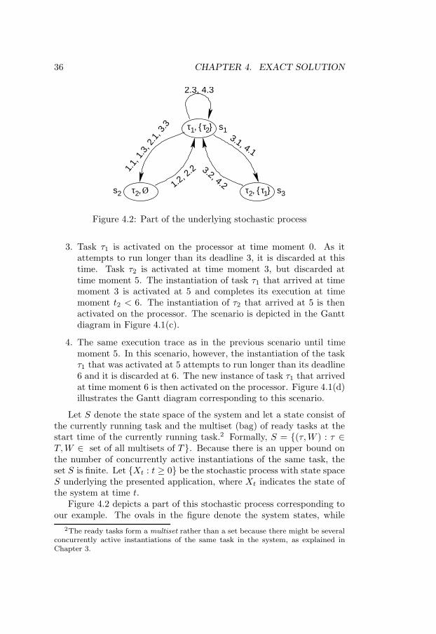
Let S denote the state space of the system and let a state consist ofthe currently running task and the multiset (bag) of ready tasks at thestart time of the currently running task.2 Formally, S = (τ, W ) : τ ∈T, W ∈ set of all multisets of T . Because there is an upper bound onthe number of concurrently active instantiations of the same task, theset S is finite. Let Xt : t ≥ 0 be the stochastic process with state spaceS underlying the presented application, where Xt indicates the state ofthe system at time t.
Figure 4.2 depicts a part of this stochastic process corresponding toour example. The ovals in the figure denote the system states, while
2The ready tasks form a multiset rather than a set because there might be severalconcurrently active instantiations of the same task in the system, as explained inChapter 3.

4.1. THE UNDERLYING STOCHASTIC PROCESS 37
time
states
t2t1
s2
s1
s3
5 630
Figure 4.3: Sample paths for scenarios 1 and 4
the arcs indicate the possible transitions between states. The states aremarked by the identifier near the ovals. The transition labels of form u.vindicate the vth taken transition in the uth scenario. The first transitionin the first scenario is briefly explained in the following. At time moment0, task τ1 starts running while τ2 is ready to run. Hence, the system stateis s1 = (τ1, τ2). In the first scenario, task τ1 completes execution attime moment t1, when the ready task τ2 is started and there are no moreready tasks. Hence, at time moment t1 the system takes the transitions1 → s2 labelled with 1.1 (the first transition in the first scenario), wheres2 = (τ2, ∅).
The solid line in Figure 4.3 depicts the sample path corresponding toscenario 1 while the dashed line represents the sample path of scenario 4.
The state holding intervals (the time intervals between two consecu-tive state transitions) correspond to residual task execution times (howmuch time it is left for a task to execute). In the general case, the ET-PDFs can be arbitrary and do not exhibit the memorylessness property.Therefore, the constructed stochastic process cannot be Markovian.
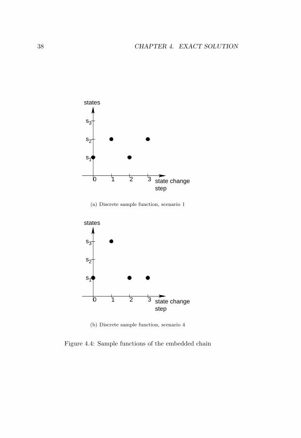
In a second attempt to find a more suitable underlying stochasticprocess, we focus on the discrete time stochastic process embedded inthe process presented above. The sample functions for the embeddeddiscrete time stochastic process are depicted in Figure 4.4. Figure 4.4(a)corresponds to scenario 1, while Figure 4.4(b) corresponds to scenario 4.The depicted discrete sample paths are strobes of the piecewise contin-uous sample paths in Figure 4.3 taken at state change moments.
Task τ1 misses its deadline when the transitions s1 → s3 or s1 →s1 occur. Therefore, the probabilities of these transitions have to be
38 CHAPTER 4. EXACT SOLUTION
states
state changestep
s2
s1
s3
30 1 2
(a) Discrete sample function, scenario 1
s2
s1
s3
30 1 2
states
state changestep
(b) Discrete sample function, scenario 4
Figure 4.4: Sample functions of the embedded chain
4.1. THE UNDERLYING STOCHASTIC PROCESS 39
τ1, τ2, 0
τ2, Ø, t1 τ2, τ1, 3
τ1, τ2, 5
τ1, τ2, 6τ , Ø, t22
s2 s3
s5 s6
s1
s4
1.3,
3.3
2.3, 4.3
1.1,
2.1
1.2, 2.2
3.1, 4.1
3.2,
4.2
Figure 4.5: Stochastic process with new state space
determined. It can be seen from the example that the transition s1 → s1
cannot occur as a first step in the scenario, but only if certain previoussteps have been performed (when, for example, the previous history iss1 → s3 → s1). Thus, it is easy to observe that the probability of atransition from a state is dependent not only on that particular statebut also on the history of previously taken transitions. Therefore, notonly the continuous time process is not Markovian, but neither is theconsidered embedded discrete time chain.
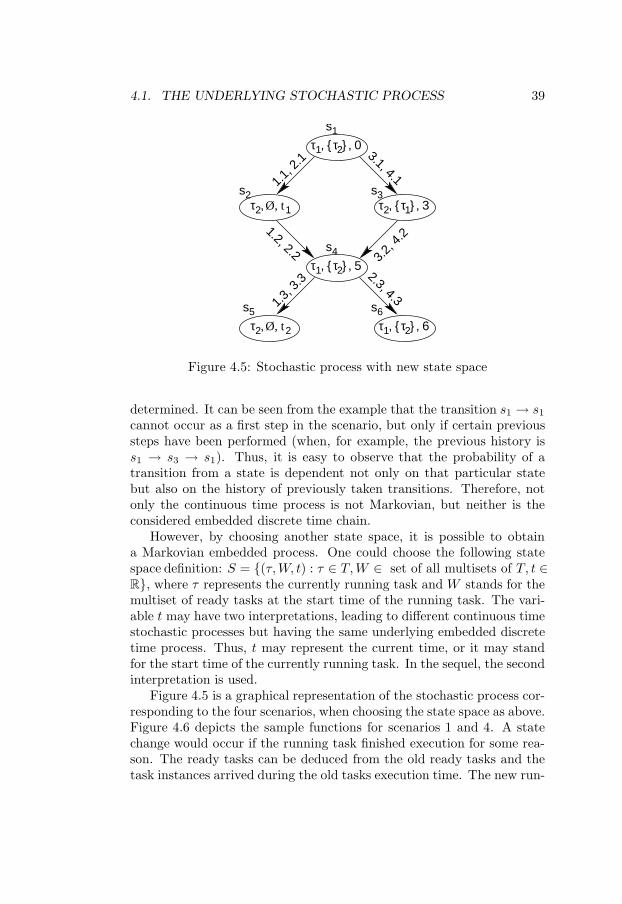
However, by choosing another state space, it is possible to obtaina Markovian embedded process. One could choose the following statespace definition: S = (τ, W, t) : τ ∈ T, W ∈ set of all multisets of T, t ∈R, where τ represents the currently running task and W stands for themultiset of ready tasks at the start time of the running task. The vari-able t may have two interpretations, leading to different continuous timestochastic processes but having the same underlying embedded discretetime process. Thus, t may represent the current time, or it may standfor the start time of the currently running task. In the sequel, the secondinterpretation is used.
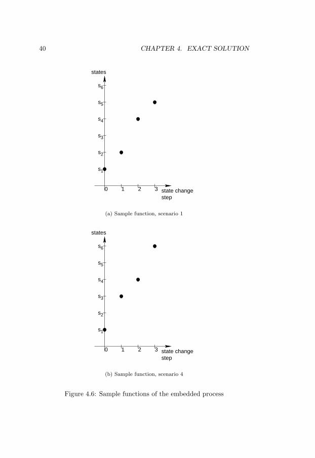
Figure 4.5 is a graphical representation of the stochastic process cor-responding to the four scenarios, when choosing the state space as above.Figure 4.6 depicts the sample functions for scenarios 1 and 4. A statechange would occur if the running task finished execution for some rea-son. The ready tasks can be deduced from the old ready tasks and thetask instances arrived during the old tasks execution time. The new run-
40 CHAPTER 4. EXACT SOLUTION
states
state changestep
s2
s1
s3
s4
s5
s6
30 1 2
(a) Sample function, scenario 1
states
state changestep
s2
s1
s3
s4
s5
s6
30 1 2
(b) Sample function, scenario 4
Figure 4.6: Sample functions of the embedded process
4.1. CONSTRUCTION AND ANALYSIS 41
ning task can be selected considering the particular scheduling policy. Asall information needed for the scheduler to choose the next running taskis present in a state, the set of possible next states can be determinedregardless of the path to the current state. Moreover, as the task starttime appears in the state information, the probability of a next state canbe determined regardless of the past states.
For example, let us consider the two states s4 = (τ1, τ2, 5) (τ1 isrunning, τ2 is ready, and τ1 has started at time moment 5), and s6 =(τ1, τ2, 6) (τ1 is running, τ2 is ready and τ1 has started at time moment6) in Figure 4.5. State s4 is left when the instantiation of τ1 which arrivedat time moment 3 and started executing at time moment 5 completesexecution for some reason. Transition s4 → s6 is taken if τ1 is discardedbecause it attempts to run longer than its deadline 6. Therefore, theprobability of this transition equals the probability of task τ1 executingfor a time interval longer than 6 − 5 = 1 time unit, i.e. P(Ex(τ1) > 1).Obviously, this probability does not depend on the past states of thesystem.
Therefore, the embedded discrete time process is Markovian and,implicitly, the continuous time process is a semi-Markov process.
As opposed to the process depicted in Figure 4.2, the time infor-mation present in the state space of the process depicted in Figure 4.5removes any ambiguity related to the exact instantiation which is run-ning in a particular state. In Figure 4.2, the state s1 corresponds to s1,s4 and s6 in Figure 4.5. In Figure 4.2, transition s1 → s1 correspondsto s4 → s6 in Figure 4.5. However, in the case of the stochastic processin Figure 4.2 it is not clear if the currently running task in state s1 (τ1)is the instantiation that has arrived at time moment 0 or the one thatarrived at 3. In the first case, the transition s1 → s1 is impossible andtherefore has probability 0, while in the second case, the transition canbe taken and has non-zero probability.
4.2 Construction and analysis of the under-lying stochastic process
Unfortunately, by introducing a continuous variable (the time) in thestate definition, the resulting continuous time stochastic process andimplicitly the embedded discrete time process become continuous (un-countable) space processes which makes their analysis very difficult. Inprinciple, there may be as many next states as many possible executiontimes the running task has. Even in the case when the task execution

42 CHAPTER 4. EXACT SOLUTION
30 1 2 4
prob
abili
ty
time
(a) ε1
30 1 2 4
prob
abili
ty
time5 6
(b) ε2
Figure 4.7: ETPDFs of tasks τ1 and τ2
time probabilities are distributed over a discrete set, the resulting un-derlying process becomes prohibitively large.
In our approach, we have grouped time moments into equivalenceclasses and, by doing so, we limited the process size explosion. Thus,practically, a set of equivalent states is represented as a single statein the stochastic process. Let us define LCM as the least commonmultiple of the task periods. For the simplicity of the exposition, letus first assume that the task instantiations are immediately discardedwhen they miss their deadlines (bi = 1, ∀1 ≤ i ≤ h). Therefore, the timemoments 0, LCM, 2 · LCM, . . . , k · LCM, . . . are renewal points of theunderlying stochastic process and the analysis can be restricted to theinterval [0, LCM).
Let us consider the same application as in the previous section, i.e.two independent tasks with respective periods 3 and 5 (LCM = 15). Thetasks are scheduled according to an EDF policy. The corresponding task
4.2. CONSTRUCTION AND ANALYSIS 43
pmi3pmi1 pmi2 pmi4 pmi5 pmi6 pmi7τ1
τ2
0 3 5 6 9 10 12 15
Figure 4.8: Priority monotonicity intervals
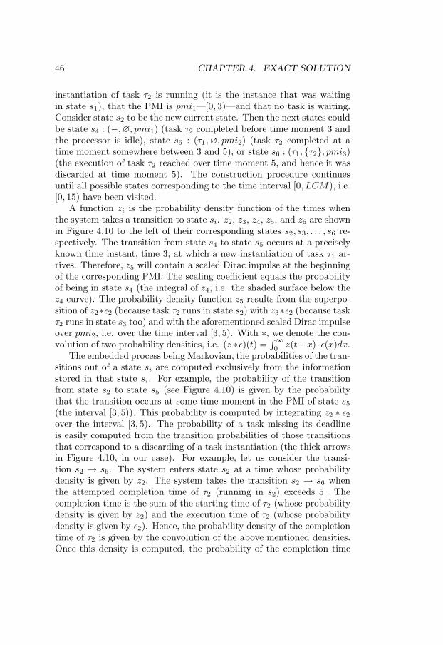
execution time probability density functions are depicted in Figure 4.7.Note that ε1 contains execution times larger than the deadline.
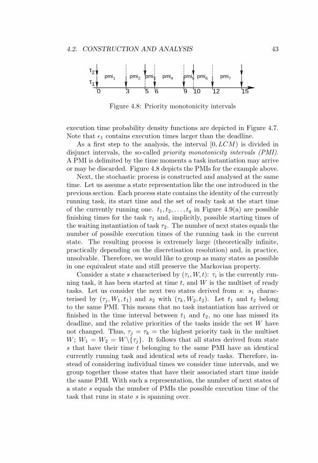
As a first step to the analysis, the interval [0, LCM) is divided indisjunct intervals, the so-called priority monotonicity intervals (PMI).A PMI is delimited by the time moments a task instantiation may arriveor may be discarded. Figure 4.8 depicts the PMIs for the example above.
Next, the stochastic process is constructed and analysed at the sametime. Let us assume a state representation like the one introduced in theprevious section. Each process state contains the identity of the currentlyrunning task, its start time and the set of ready task at the start timeof the currently running one. t1, t2, . . . , tq in Figure 4.9(a) are possiblefinishing times for the task τ1 and, implicitly, possible starting times ofthe waiting instantiation of task τ2. The number of next states equals thenumber of possible execution times of the running task in the currentstate. The resulting process is extremely large (theoretically infinite,practically depending on the discretisation resolution) and, in practice,unsolvable. Therefore, we would like to group as many states as possiblein one equivalent state and still preserve the Markovian property.
Consider a state s characterised by (τi, W, t): τi is the currently run-ning task, it has been started at time t, and W is the multiset of readytasks. Let us consider the next two states derived from s: s1 charac-terised by (τj , W1, t1) and s2 with (τk, W2, t2). Let t1 and t2 belongto the same PMI. This means that no task instantiation has arrived orfinished in the time interval between t1 and t2, no one has missed itsdeadline, and the relative priorities of the tasks inside the set W havenot changed. Thus, τj = τk = the highest priority task in the multisetW ; W1 = W2 = W\τj. It follows that all states derived from states that have their time t belonging to the same PMI have an identicalcurrently running task and identical sets of ready tasks. Therefore, in-stead of considering individual times we consider time intervals, and wegroup together those states that have their associated start time insidethe same PMI. With such a representation, the number of next states ofa state s equals the number of PMIs the possible execution time of thetask that runs in state s is spanning over.

44 CHAPTER 4. EXACT SOLUTION
τ1, τ2, 0
τ2, Ø, t1 tk+1 tqτ2, τ1, τ2, Ø, t τ2, Ø, t τ2, τ12 k , ...
(a) Individual task completion times
τ1, τ2, pmi1
τ2, Ø, pmi1 τ2, τ1, pmi2
(b) Intervals containing task completion times
Figure 4.9: State encoding
4.2. CONSTRUCTION AND ANALYSIS 45
time
prob
abili
ty
3 4 5 6 time
prob
abili
ty
5 643 time
prob
abili
ty
τ1 , τ2 , pmi1
−, Ø,pmi1 τ1 , τ2 , pmi3
τ2 , τ1 , pmi2τ2 , Ø, pmi1
τ1 , Ø,pmi2
s1
s2
s4 s5 s6
s3
z3
z5 z6
1 2 3 4 time
prob
abili
ty
z2
1 2 3 4 time
prob
abili
ty
z4
1 2 3 4
Figure 4.10: Stochastic process example
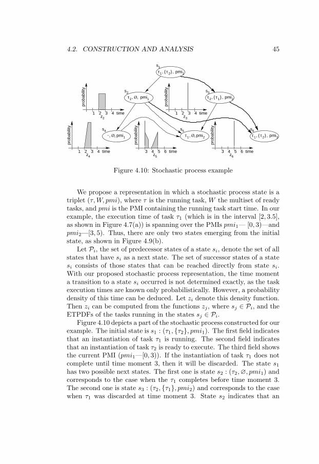
We propose a representation in which a stochastic process state is atriplet (τ, W, pmi), where τ is the running task, W the multiset of readytasks, and pmi is the PMI containing the running task start time. In ourexample, the execution time of task τ1 (which is in the interval [2, 3.5],as shown in Figure 4.7(a)) is spanning over the PMIs pmi1— [0, 3)—andpmi2—[3, 5). Thus, there are only two states emerging from the initialstate, as shown in Figure 4.9(b).
Let Pi, the set of predecessor states of a state si, denote the set of allstates that have si as a next state. The set of successor states of a statesi consists of those states that can be reached directly from state si.With our proposed stochastic process representation, the time momenta transition to a state si occurred is not determined exactly, as the taskexecution times are known only probabilistically. However, a probabilitydensity of this time can be deduced. Let zi denote this density function.Then zi can be computed from the functions zj, where sj ∈ Pi, and theETPDFs of the tasks running in the states sj ∈ Pi.
Figure 4.10 depicts a part of the stochastic process constructed for ourexample. The initial state is s1 : (τ1, τ2, pmi1). The first field indicatesthat an instantiation of task τ1 is running. The second field indicatesthat an instantiation of task τ2 is ready to execute. The third field showsthe current PMI (pmi1—[0, 3)). If the instantiation of task τ1 does notcomplete until time moment 3, then it will be discarded. The state s1
has two possible next states. The first one is state s2 : (τ2, ∅, pmi1) andcorresponds to the case when the τ1 completes before time moment 3.The second one is state s3 : (τ2, τ1, pmi2) and corresponds to the casewhen τ1 was discarded at time moment 3. State s2 indicates that an
46 CHAPTER 4. EXACT SOLUTION
instantiation of task τ2 is running (it is the instance that was waitingin state s1), that the PMI is pmi1—[0, 3)—and that no task is waiting.Consider state s2 to be the new current state. Then the next states couldbe state s4 : (−, ∅, pmi1) (task τ2 completed before time moment 3 andthe processor is idle), state s5 : (τ1, ∅, pmi2) (task τ2 completed at atime moment somewhere between 3 and 5), or state s6 : (τ1, τ2, pmi3)(the execution of task τ2 reached over time moment 5, and hence it wasdiscarded at time moment 5). The construction procedure continuesuntil all possible states corresponding to the time interval [0, LCM), i.e.[0, 15) have been visited.
A function zi is the probability density function of the times whenthe system takes a transition to state si. z2, z3, z4, z5, and z6 are shownin Figure 4.10 to the left of their corresponding states s2, s3, . . . , s6 re-spectively. The transition from state s4 to state s5 occurs at a preciselyknown time instant, time 3, at which a new instantiation of task τ1 ar-rives. Therefore, z5 will contain a scaled Dirac impulse at the beginningof the corresponding PMI. The scaling coefficient equals the probabilityof being in state s4 (the integral of z4, i.e. the shaded surface below thez4 curve). The probability density function z5 results from the superpo-sition of z2∗ε2 (because task τ2 runs in state s2) with z3∗ε2 (because taskτ2 runs in state s3 too) and with the aforementioned scaled Dirac impulseover pmi2, i.e. over the time interval [3, 5). With ∗, we denote the con-volution of two probability densities, i.e. (z ∗ ε)(t) =
∫∞0 z(t−x) ·ε(x)dx.
The embedded process being Markovian, the probabilities of the tran-sitions out of a state si are computed exclusively from the informationstored in that state si. For example, the probability of the transitionfrom state s2 to state s5 (see Figure 4.10) is given by the probabilitythat the transition occurs at some time moment in the PMI of state s5
(the interval [3, 5)). This probability is computed by integrating z2 ∗ ε2over the interval [3, 5). The probability of a task missing its deadlineis easily computed from the transition probabilities of those transitionsthat correspond to a discarding of a task instantiation (the thick arrowsin Figure 4.10, in our case). For example, let us consider the transi-tion s2 → s6. The system enters state s2 at a time whose probabilitydensity is given by z2. The system takes the transition s2 → s6 whenthe attempted completion time of τ2 (running in s2) exceeds 5. Thecompletion time is the sum of the starting time of τ2 (whose probabilitydensity is given by z2) and the execution time of τ2 (whose probabilitydensity is given by ε2). Hence, the probability density of the completiontime of τ2 is given by the convolution of the above mentioned densities.Once this density is computed, the probability of the completion time

4.3. MEMORY EFFICIENT ANALYSIS METHOD 47
being larger than 5 is easily computed by integrating the result of theconvolution over the interval [5,∞).
As it can be seen, by using the PMI approach, some process stateshave more than one incident arc, thus keeping the graph “narrow”. Thisis because, as mentioned, one process state in our representation capturesseveral possible states of a representation considering individual times(see Figure 4.9(a)).
Because the number of states grows rapidly and each state has tostore its probability density function, the memory space required tostore the whole process can become prohibitively large. Our solutionto mastering memory complexity is to perform the stochastic processconstruction and analysis simultaneously. As each arrow updates thetime probability density of the state it leads to, the process has to beconstructed in topological order. The result of this procedure is thatthe process is never stored entirely in memory but rather that a slidingwindow of states is used for analysis. For the example in Figure 4.10, theconstruction starts with state s1. After its next states (s2 and s3) arecreated, their corresponding transition probabilities determined and thepossible discarding probabilities accounted for, state s1 can be removedfrom memory. Next, one of the states s2 and s3 is taken as current state,let us consider state s2. The procedure is repeated, states s4, s5 and s6
are created and state s2 removed. At this moment, the arcs emergingfrom states s3 and s4 have not yet been created. Consequently, onewould think that any of the states s3, s4, s5, and s6 can be selected forcontinuation of the analysis. Obviously, this is not the case, as not allthe information needed in order to handle states s5 and s6 are computed(in particular those coming from s3 and s4). Thus, only states s3 ands4 are possible alternatives for the continuation of the analysis in topo-logical order. The next section discusses the criteria for selection of thecorrect state to continue with.
4.3 Memory efficient analysis method
As shown in the example in Section 4.2, only a sliding window of states issimultaneously kept in memory. All states belonging to the sliding win-dow are stored in a priority queue. The key to the process constructionin topological order lies in the order in which the states are extractedfrom this queue. First, observe that it is impossible for an arc to leadfrom a state with a PMI number u to a state with a PMI number v sothat v < u (there are no arcs back in time). Hence, a first criterion forselecting a state from the queue is to select the one with the smallest

48 CHAPTER 4. EXACT SOLUTION
1
2
3
4
5 6
Figure 4.11: State selection order
PMI number. A second criterion determines which state has to be se-lected out of those with the same PMI number. Note that inside a PMIno new task instantiation can arrive, and that the task ordering accord-ing to their priorities is unchanged. Thus, it is impossible that the nextstate sk of a current state sj would be one that contains waiting tasksof higher priority than those waiting in sj. Hence, the second criterionreads: among states with the same PMI, one should choose the one withthe waiting task of highest priority. Figure 4.11 illustrates the algorithmon the example given in Section 4.2 (Figure 4.10). The shades of thestates denote their PMI number. The lighter the shade, the smaller thePMI number. The numbers near the states denote the sequence in whichthe states are extracted from the queue and processed.
4.4 Flexible discarding
The examples considered so far dealt with applications where a late taskis immediately discarded (bi = 1, 1 ≤ i ≤ h, i.e. at most one activeinstance of each task graph is allowed at any moment of time).
In this case, all the late tasks are discarded at the time momentsLCM, 2 ·LCM, . . . , k ·LCM, . . . because at these moments new instan-tiations of all tasks arrive. The system behaves at these time moments asif it has just been started. The time moments k ·LCM , k ∈ N are calledrenewal points. The system states at the renewal points are equivalentto the initial state which is unique and deterministically known. Thus,the behaviour of the system over the intervals [k ·LCM, (k + 1) ·LCM),k ∈ N, is statistically equivalent to the behaviour over the time interval
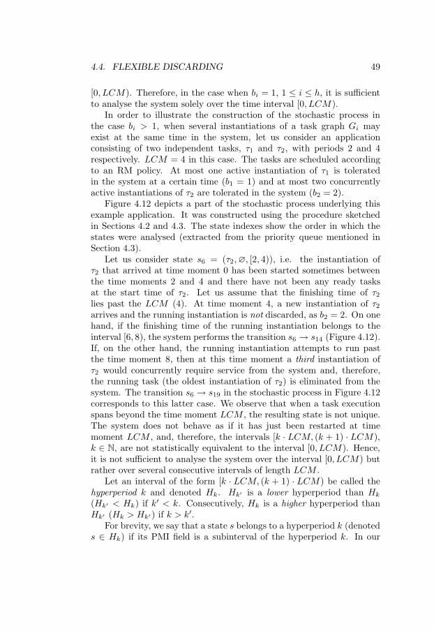
4.4. FLEXIBLE DISCARDING 49
[0, LCM). Therefore, in the case when bi = 1, 1 ≤ i ≤ h, it is sufficientto analyse the system solely over the time interval [0, LCM).
In order to illustrate the construction of the stochastic process inthe case bi > 1, when several instantiations of a task graph Gi mayexist at the same time in the system, let us consider an applicationconsisting of two independent tasks, τ1 and τ2, with periods 2 and 4respectively. LCM = 4 in this case. The tasks are scheduled accordingto an RM policy. At most one active instantiation of τ1 is toleratedin the system at a certain time (b1 = 1) and at most two concurrentlyactive instantiations of τ2 are tolerated in the system (b2 = 2).
Figure 4.12 depicts a part of the stochastic process underlying thisexample application. It was constructed using the procedure sketchedin Sections 4.2 and 4.3. The state indexes show the order in which thestates were analysed (extracted from the priority queue mentioned inSection 4.3).
Let us consider state s6 = (τ2, ∅, [2, 4)), i.e. the instantiation ofτ2 that arrived at time moment 0 has been started sometimes betweenthe time moments 2 and 4 and there have not been any ready tasksat the start time of τ2. Let us assume that the finishing time of τ2
lies past the LCM (4). At time moment 4, a new instantiation of τ2
arrives and the running instantiation is not discarded, as b2 = 2. On onehand, if the finishing time of the running instantiation belongs to theinterval [6, 8), the system performs the transition s6 → s14 (Figure 4.12).If, on the other hand, the running instantiation attempts to run pastthe time moment 8, then at this time moment a third instantiation ofτ2 would concurrently require service from the system and, therefore,the running task (the oldest instantiation of τ2) is eliminated from thesystem. The transition s6 → s19 in the stochastic process in Figure 4.12corresponds to this latter case. We observe that when a task executionspans beyond the time moment LCM , the resulting state is not unique.The system does not behave as if it has just been restarted at timemoment LCM , and, therefore, the intervals [k · LCM, (k + 1) · LCM),k ∈ N, are not statistically equivalent to the interval [0, LCM). Hence,it is not sufficient to analyse the system over the interval [0, LCM) butrather over several consecutive intervals of length LCM .
Let an interval of the form [k · LCM, (k + 1) · LCM) be called thehyperperiod k and denoted Hk. Hk′ is a lower hyperperiod than Hk
(Hk′ < Hk) if k′ < k. Consecutively, Hk is a higher hyperperiod thanHk′ (Hk > Hk′ ) if k > k′.
For brevity, we say that a state s belongs to a hyperperiod k (denoteds ∈ Hk) if its PMI field is a subinterval of the hyperperiod k. In our
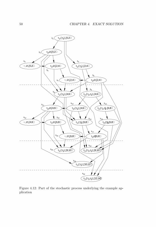
50 CHAPTER 4. EXACT SOLUTION
τ1,τ2,[0,2)
τ1,τ2,[2,4)
τ2,Ø,[0,2)
τ1,Ø,[2,4)
τ2,Ø,[2,4)−, Ø,[2,4)
−, Ø,[0,2)
τ2,
τ1,
τ2,
τ1,τ2,[8,10) τ1,τ2,τ2,[8,10)
s1
s3
s10
s12
s17
s18
s30
20s
τ1,τ2,[10,12)s25
τ1,τ2,τ2,[4,6)τ1,τ2
Ø
Ø−, Ø τ1,τ2
τ2,τ2 τ1,τ2,τ2
τ2,τ2
−, Ø Ø
,[4,6)
,[4,6) ,[4,6) ,[6,8)
,[4,6) ,[6,8) ,[6,8) ,[6,8)
,[6,8) ,[6,8)
τ1,τ2,τ2,[12,14)
s2
s5
s4
s6
s7
s8s9
s11s13
s14 s15s16
s19
Figure 4.12: Part of the stochastic process underlying the example ap-plication
4.4. FLEXIBLE DISCARDING 51
example, three hyperperiods are considered, H0 = [0, 4), H1 = [4, 8), andH2 = [8, 12). In the stochastic process in Figure 4.12, s1, s2, . . . , s7 ∈ H0,s8, s9, . . . , s18 ∈ H1, and s19, s20, s25 ∈ H2 (node that not all states havebeen depicted in Figure 4.12).
In general, let us consider a state s and let Ps be the set of itspredecessor states. Let k denote the order of the state s defined as thelowest hyperperiod of the states in Ps (k = minj : s′ ∈ Hj , s
′ ∈ Ps).If s ∈ Hk and s is of order k′ and k′ < k, then s is a back state.In ourexample, s8, s9, s14, and s19 are back states of order 0, while s20, s25
and s30 are back states of order 1.Obviously, there cannot be any transition from a state belonging to
a hyperperiod H to a state belonging to a lower hyperperiod than H(s → s′, s ∈ Hk, s′ ∈ Hk′ ⇒ Hk ≤ Hk′ ). Consequently, the set S ofall states belonging to a hyperperiod Hk can be constructed from theback states of an order smaller than k. We say that S is generatedby the aforementioned back states. For example, the set of all statess8, s9, . . . , s18 ∈ H1 can be derived from the back states s8, s9, s14, ands19 of order 0. The intuition behind this is that back states are inheritingall the needed information across the border between hyperperiods.
Before continuing our discussion, we have to introduce the notion ofsimilarity between states. We say that two states si and sj are similar(si ∼ sj) if
1. The task which is running in si and sj is the same,
2. The multiset of ready tasks in si and sj is the same,
3. The PMIs in the two states differ only by a multiple of LCM ,
4. zi = zj (zi is the probability density function of the times whenthe system takes a transition to si).
Let us consider the construction and analysis of the stochastic pro-cess, as described in Sections 4.2 and 4.3. Let us consider the momentx, when the last state belonging to a certain hyperperiod Hk has beeneliminated from the sliding window. Rk is the set of back states stored inthe sliding window at the moment x. Let the analysis proceed with thestates of the hyperperiod Hk+1 and let us consider the moment y whenthe last state belonging to Hk+1 has been eliminated from the slidingwindow. Let Rk+1 be the set of back states stored in the sliding windowat moment y.
If the sets Rk and Rk+1 contain pairwise similar states, then it is guar-anteed that Rk and Rk+1 generate identical stochastic processes during
52 CHAPTER 4. EXACT SOLUTION
the rest of the analysis procedure (as stated, at a certain moment the setof back states univocally determines the rest of the stochastic process).In our example, R0 = s8, s9, s14, s19 and R1 = s19, s20, s25, s30. Ifs8 ∼ s19, s9 ∼ s20, s14 ∼ s25, and s19 ∼ s30 then the analysis processmay stop as it reached convergence.
Consequently, the analysis proceeds by considering states of consec-utive hyperperiods until the information captured by the back states inthe sliding window does not change anymore. Whenever the underlyingstochastic process has a steady state, this steady state is guaranteed tobe found.
4.5 Construction and analysis algorithm
The analysis is performed in two phases:
1. Divide the interval [0, LCM) in PMIs,
2. Construct the stochastic process in topological order and analyseit.
The concept of PMI (called in their paper “state”) was introduced byZhou et al.[ZHS99] in a different context, unrelated to the constructionof a stochastic process. Let Ai denote the set of time moments in theinterval [0, LCM) when a new instantiation of the task τi arrives and letA denote the union of all Ai. Let Di denote the set of absolute deadlinesof the instantiations of task τi in the interval [0, LCM), and D be theunion of all Di . Consequently,
Ai = x : x = k · πi, 0 ≤ k < LCM/πiDi = x : x = δi + k · πi, 0 ≤ k < LCM/πi
If the deadlines are assumed to equal the periods, then Di = Ai (themoment 0 is assumed to be the deadline of the instantiation arrived atmoment −πi.
Let H = A ∪ D. If H is sorted in ascending order of the time mo-ments, then a priority monotonicity interval is the interval between twoconsecutive time moments in H . The last PMI is the interval betweenthe greatest element in H and LCM . The only restriction imposed onthe scheduling policies accepted by our approach is that inside a PMI theordering of tasks according to their priorities is not allowed to change.The consequence of this assumption is that the next state can be deter-mined, no matter when the currently running task completes within the
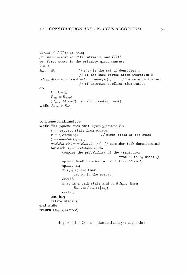
4.5. CONSTRUCTION AND ANALYSIS ALGORITHM 53
divide [0, LCM) in PMIs;pmi no = number of PMIs between 0 and LCM ;put first state in the priority queue pqueue;k = 1;Rold = ∅; // Rold is the set of densities z
// of the back states after iteration k(Rnew, Missed) = construct and analyse(); // Missed is the set
// of expected deadline miss ratios
dok = k + 1;Rold = Rnew;(Rnew , Missed) = construct and analyse();
while Rnew 6= Rold;
construct and analyse:while ∃s ∈ pqueue such that s.pmi ≤ pmi no do
sj = extract state from pqueue;τi = sj .running; // first field of the state
ξ = convolute(εi, zj);nextstatelist = next states(sj); // consider task dependencies!
for each su ∈ nextstatelist docompute the probability of the transition
from sj to su using ξ;update deadline miss probabilities Missed;update zu;if su 6∈ pqueue then
put su in the pqueue;end if;if su is a back state and su 6∈ Rnew then
Rnew = Rnew ∪ su;end if;
end for;delete state sj;
end while;return (Rnew , Missed);
Figure 4.13: Construction and analysis algorithm
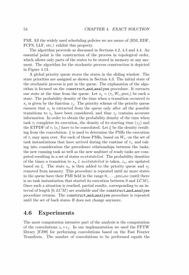
54 CHAPTER 4. EXACT SOLUTION
PMI. All the widely used scheduling policies we are aware of (RM, EDF,FCFS, LLF, etc.) exhibit this property.
The algorithm proceeds as discussed in Sections 4.2, 4.3 and 4.4. Anessential point is the construction of the process in topological order,which allows only parts of the states to be stored in memory at any mo-ment. The algorithm for the stochastic process construction is depictedin Figure 4.13.
A global priority queue stores the states in the sliding window. Thestate priorities are assigned as shown in Section 4.3. The initial state ofthe stochastic process is put in the queue. The explanation of the algo-rithm is focused on the construct and analyse procedure. It extractsone state at the time from the queue. Let sj = (τi, Wi, pmii) be such astate. The probability density of the time when a transition occurred tosj is given by the function zj. The priority scheme of the priority queueensures that sj is extracted from the queue only after all the possibletransitions to sj have been considered, and thus zj contains accurateinformation. In order to obtain the probability density of the time whentask τi completes its execution, the density of its starting time (zj) andthe ETPDF of τi (εi) have to be convoluted. Let ξ be the density result-ing from the convolution. ξ is used to determine the PMIs the executionof τi may span over. For each of those PMIs, based on Wi, on the set oftask instantiations that have arrived during the runtime of τi, and tak-ing into consideration the precedence relationships between the tasks,the new running task as well as the new multiset of ready tasks are com-puted resulting in a set of states nextstatelist. The probability densitiesof the times a transition to su ∈ nextstatelist is taken, zu, are updatedbased on ξ. The state su is then added to the priority queue and sj
removed from memory. This procedure is repeated until no more statesin the queue have their PMI field in the range 0, . . . , pmi no (until thereis no task instantiation that started its execution between 0 and LCM).Once such a situation is reached, partial results, corresponding to an in-terval of length [0, LCM) are available and the construct and analyseprocedure returns. The construct and analyse procedure is repeateduntil the set of back states R does not change anymore.
4.6 Experiments
The most computation intensive part of the analysis is the computationof the convolutions zi ∗ εj . In our implementation we used the FFTWlibrary [FJ98] for performing convolutions based on the Fast FourierTransform. The number of convolutions to be performed equals the
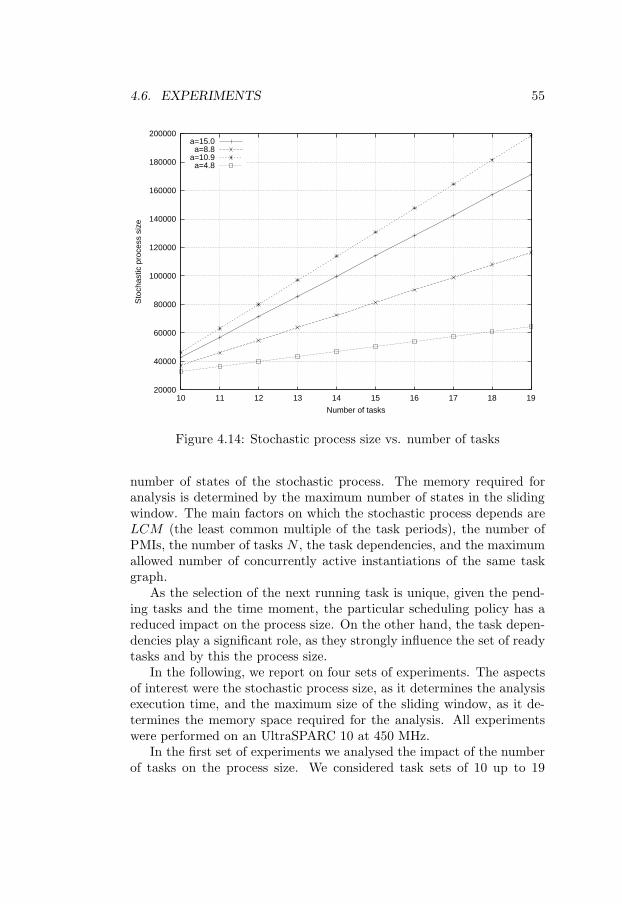
4.6. EXPERIMENTS 55
20000
40000
60000
80000
100000
120000
140000
160000
180000
200000
10 11 12 13 14 15 16 17 18 19
Sto
chas
tic p
roce
ss s
ize
Number of tasks
a=15.0a=8.8
a=10.9a=4.8
Figure 4.14: Stochastic process size vs. number of tasks
number of states of the stochastic process. The memory required foranalysis is determined by the maximum number of states in the slidingwindow. The main factors on which the stochastic process depends areLCM (the least common multiple of the task periods), the number ofPMIs, the number of tasks N , the task dependencies, and the maximumallowed number of concurrently active instantiations of the same taskgraph.
As the selection of the next running task is unique, given the pend-ing tasks and the time moment, the particular scheduling policy has areduced impact on the process size. On the other hand, the task depen-dencies play a significant role, as they strongly influence the set of readytasks and by this the process size.
In the following, we report on four sets of experiments. The aspectsof interest were the stochastic process size, as it determines the analysisexecution time, and the maximum size of the sliding window, as it de-termines the memory space required for the analysis. All experimentswere performed on an UltraSPARC 10 at 450 MHz.
In the first set of experiments we analysed the impact of the numberof tasks on the process size. We considered task sets of 10 up to 19

56 CHAPTER 4. EXACT SOLUTION
0
2000
4000
6000
8000
10000
12000
10 11 12 13 14 15 16 17 18 19
Slid
ing
win
dow
siz
e [n
umbe
r of
sta
tes]
Number of tasks
a=15.0a=8.8
a=10.9a=4.8
Figure 4.15: Size of the sliding window of states vs. number of tasks
independent tasks. LCM , the least common multiple of the task periods,was 360 for all task sets. We repeated the experiment four times foraverage values of the task periods a = 15.0, 10.9, 8.8, and 4.8 (keepingLCM = 360). The results are shown in Figure 4.14. Figure 4.15 depictsthe maximum size of the sliding window for the same task sets. As it canbe seen from the diagram, the increase, both of the process size and of thesliding window, is linear. The steepness of the curves depends on the taskperiods (which influence the number of PMIs). It is important to noticethe big difference between the process size and the maximum numberof states in the sliding window. In the case for 19 tasks, for example,the process size is between 64356 and 198356 while the dimension of thesliding window varies between 373 and 11883 (16 to 172 times smaller).The reduction factor of the sliding window compared to the process sizewas between 15 and 1914, considering all our experiments.
In the second set of experiments we analysed the impact of the ap-plication period LCM (the least common multiple of the task periods)on the process size. We considered 784 sets, each of 20 independenttasks. The task periods were chosen such that LCM takes values in the
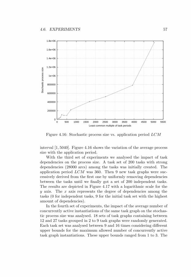
4.6. EXPERIMENTS 57
0
200000
400000
600000
800000
1e+06
1.2e+06
1.4e+06
1.6e+06
1.8e+06
0 500 1000 1500 2000 2500 3000 3500 4000 4500 5000 5500
Sto
chas
tic p
roce
ss s
ize
Least common multiple of task periods
Figure 4.16: Stochastic process size vs. application period LCM
interval [1, 5040]. Figure 4.16 shows the variation of the average processsize with the application period.
With the third set of experiments we analysed the impact of taskdependencies on the process size. A task set of 200 tasks with strongdependencies (28000 arcs) among the tasks was initially created. Theapplication period LCM was 360. Then 9 new task graphs were suc-cessively derived from the first one by uniformly removing dependenciesbetween the tasks until we finally got a set of 200 independent tasks.The results are depicted in Figure 4.17 with a logarithmic scale for they axis. The x axis represents the degree of dependencies among thetasks (0 for independent tasks, 9 for the initial task set with the highestamount of dependencies).
In the fourth set of experiments, the impact of the average number ofconcurrently active instantiations of the same task graph on the stochas-tic process size was analysed. 18 sets of task graphs containing between12 and 27 tasks grouped in 2 to 9 task graphs were randomly generated.Each task set was analysed between 9 and 16 times considering differentupper bounds for the maximum allowed number of concurrently activetask graph instantiations. These upper bounds ranged from 1 to 3. The
58 CHAPTER 4. EXACT SOLUTION
1000
10000
100000
1e+06
0 1 2 3 4 5 6 7 8 9
Sto
chas
tic p
roce
ss s
ize
Dependency degree
Figure 4.17: Stochastic process size vs. task dependency degree
results were averaged for the same number of tasks. The dependency ofthe underlying stochastic process size as a function of the average of themaximum allowed number of instantiations of the same task graph thatare concurrently active is plotted in Figure 4.18. Note that the y-axisis logarithmic. Different curves correspond to different sizes of the con-sidered task sets. It can be observed that the stochastic process size isapproximately linear in the average of the maximum allowed number ofconcurrently active instantiations of the same task graph.
As mentioned, the execution time for the analysis algorithm strictlydepends on the process size. Therefore, we showed all the results interms of this parameter. For the set of 200 independent tasks used inthe third experiment (process size 1126517, Figure 4.17) the analysistime was 745 seconds. In the case of the same 200 tasks with strongdependencies (process size 2178) the analysis took 1.4 seconds.
Finally, we considered an example from the mobile communicationarea. Figure 4.19 depicts a set of 8 tasks that co-operate in order todecode the digital bursts corresponding to a GSM 900 signalling channel.The incoming bursts are demodulated by the demodulation task, basedon the frequency indexes generated by the frequency hopping task. The
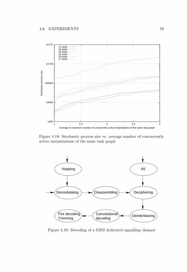
4.6. EXPERIMENTS 59
1000
10000
100000
1e+06
1e+07
1 1.5 2 2.5 3
Sto
chas
tic p
roce
ss s
ize
Average of maximum number of concurrently active instantiations of the same task graph
12 tasks15 tasks18 tasks21 tasks24 tasks27 tasks
Figure 4.18: Stochastic process size vs. average number of concurrentlyactive instantiations of the same task graph
Demodulating Disassembling Deciphering
A5
Fire decodingTrimming
Hopping
DeinterleavingConvolutionaldecoding
Figure 4.19: Decoding of a GSM dedicated signalling channel
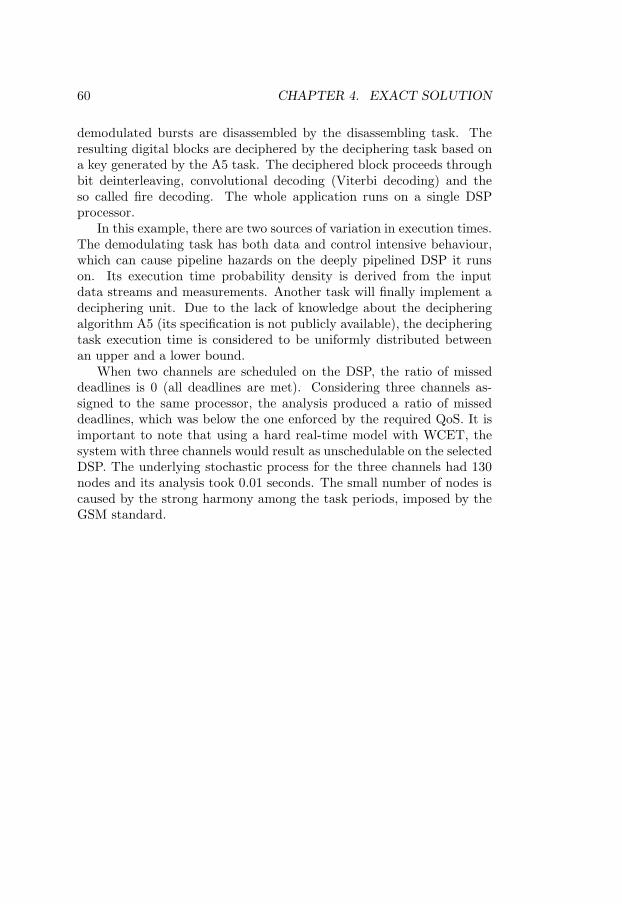
60 CHAPTER 4. EXACT SOLUTION
demodulated bursts are disassembled by the disassembling task. Theresulting digital blocks are deciphered by the deciphering task based ona key generated by the A5 task. The deciphered block proceeds throughbit deinterleaving, convolutional decoding (Viterbi decoding) and theso called fire decoding. The whole application runs on a single DSPprocessor.
In this example, there are two sources of variation in execution times.The demodulating task has both data and control intensive behaviour,which can cause pipeline hazards on the deeply pipelined DSP it runson. Its execution time probability density is derived from the inputdata streams and measurements. Another task will finally implement adeciphering unit. Due to the lack of knowledge about the decipheringalgorithm A5 (its specification is not publicly available), the decipheringtask execution time is considered to be uniformly distributed betweenan upper and a lower bound.
When two channels are scheduled on the DSP, the ratio of misseddeadlines is 0 (all deadlines are met). Considering three channels as-signed to the same processor, the analysis produced a ratio of misseddeadlines, which was below the one enforced by the required QoS. It isimportant to note that using a hard real-time model with WCET, thesystem with three channels would result as unschedulable on the selectedDSP. The underlying stochastic process for the three channels had 130nodes and its analysis took 0.01 seconds. The small number of nodes iscaused by the strong harmony among the task periods, imposed by theGSM standard.

Chapter 5
An ApproximateSolution forSchedulability Analysis:The Multi-processorCase
When analysing multi-processor applications, one approach could be todecompose the analysis problem into several subproblems, each of themanalysing the tasks mapped on one of the processors. We could attemptto apply the exact approach presented in the previous chapter in orderto solve each of the subproblems. Unfortunately, in the case of multi-processors and with the assumption of data dependencies among tasks,this approach cannot be applied. The reason is that the set of readytasks cannot be determined based solely on the information regardingthe tasks mapped on the processor under consideration.
An alternative approach would be to consider all the tasks and toconstruct the global state space of the underlying stochastic processaccordingly. In principle, the exact approach presented in the previouschapter could be applied in this case. However, the number of possibleexecution traces, and implicitly the stochastic process, explodes due tothe parallelism provided by the application platform. As shown, theanalysis has to store the probability distributions zi for each processstate in the sliding window of states, leading to large amounts of needed
61
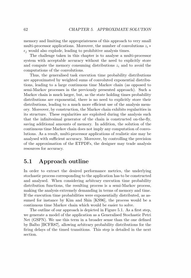
62 CHAPTER 5. APPROXIMATE SOLUTION
memory and limiting the appropriateness of this approach to very smallmulti-processor applications. Moreover, the number of convolutions zi ∗εj would also explode, leading to prohibitive analysis times.
The challenge taken in this chapter is to analyse a multi-processorsystem with acceptable accuracy without the need to explicitly storeand compute the memory consuming distributions zi and to avoid thecomputations of the convolutions.
Thus, the generalised task execution time probability distributionsare approximated by weighted sums of convoluted exponential distribu-tions, leading to a large continuous time Markov chain (as opposed tosemi-Markov processes in the previously presented approach). Such aMarkov chain is much larger, but, as the state holding times probabilitydistributions are exponential, there is no need to explicitly store theirdistributions, leading to a much more efficient use of the analysis mem-ory. Moreover, by construction, the Markov chain exhibits regularities inits structure. These regularities are exploited during the analysis suchthat the infinitesimal generator of the chain is constructed on-the-fly,saving additional amounts of memory. In addition, the solution of thecontinuous time Markov chain does not imply any computation of convo-lutions. As a result, multi-processor applications of realistic size may beanalysed with sufficient accuracy. Moreover, by controlling the precisionof the approximation of the ETPDFs, the designer may trade analysisresources for accuracy.
5.1 Approach outline
In order to extract the desired performance metrics, the underlyingstochastic process corresponding to the application has to be constructedand analysed. When considering arbitrary execution time probabilitydistribution functions, the resulting process is a semi-Markov process,making the analysis extremely demanding in terms of memory and time.If the execution time probabilities were exponentially distributed, as as-sumed for instance by Kim and Shin [KS96], the process would be acontinuous time Markov chain which would be easier to solve.
The outline of our approach is depicted in Figure 5.1. As a first step,we generate a model of the application as a Generalised Stochastic PetriNet (GSPN). We use this term in a broader sense than the one definedby Balbo [BCFR87], allowing arbitrary probability distributions for thefiring delays of the timed transitions. This step is detailed in the nextsection.
5.1. APPROACH OUTLINE 63
Application(set of graphs of taskswith arbitrary ETPDFs)
GSPN modelgeneration
GSPN model
CTMC construction
CTMC
Analysis of the CTMC
Results(percentage of missed
deadlines)
Approximation of thearbitrary ETPDFs withCoxian distributions
Coxian distributionscorresponding toarbitrary ETPDFs
step 1
step 2
step 3
step 4
Figure 5.1: Approach outline
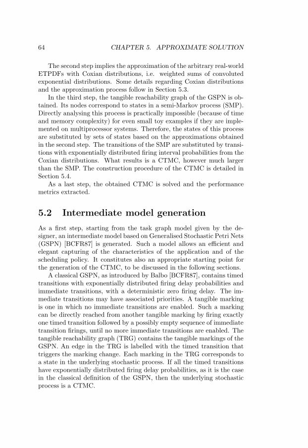
64 CHAPTER 5. APPROXIMATE SOLUTION
The second step implies the approximation of the arbitrary real-worldETPDFs with Coxian distributions, i.e. weighted sums of convolutedexponential distributions. Some details regarding Coxian distributionsand the approximation process follow in Section 5.3.
In the third step, the tangible reachability graph of the GSPN is ob-tained. Its nodes correspond to states in a semi-Markov process (SMP).Directly analysing this process is practically impossible (because of timeand memory complexity) for even small toy examples if they are imple-mented on multiprocessor systems. Therefore, the states of this processare substituted by sets of states based on the approximations obtainedin the second step. The transitions of the SMP are substituted by transi-tions with exponentially distributed firing interval probabilities from theCoxian distributions. What results is a CTMC, however much largerthan the SMP. The construction procedure of the CTMC is detailed inSection 5.4.
As a last step, the obtained CTMC is solved and the performancemetrics extracted.
5.2 Intermediate model generation
As a first step, starting from the task graph model given by the de-signer, an intermediate model based on Generalised Stochastic Petri Nets(GSPN) [BCFR87] is generated. Such a model allows an efficient andelegant capturing of the characteristics of the application and of thescheduling policy. It constitutes also an appropriate starting point forthe generation of the CTMC, to be discussed in the following sections.
A classical GSPN, as introduced by Balbo [BCFR87], contains timedtransitions with exponentially distributed firing delay probabilities andimmediate transitions, with a deterministic zero firing delay. The im-mediate transitions may have associated priorities. A tangible markingis one in which no immediate transitions are enabled. Such a markingcan be directly reached from another tangible marking by firing exactlyone timed transition followed by a possibly empty sequence of immediatetransition firings, until no more immediate transitions are enabled. Thetangible reachability graph (TRG) contains the tangible markings of theGSPN. An edge in the TRG is labelled with the timed transition thattriggers the marking change. Each marking in the TRG corresponds toa state in the underlying stochastic process. If all the timed transitionshave exponentially distributed firing delay probabilities, as it is the casein the classical definition of the GSPN, then the underlying stochasticprocess is a CTMC.
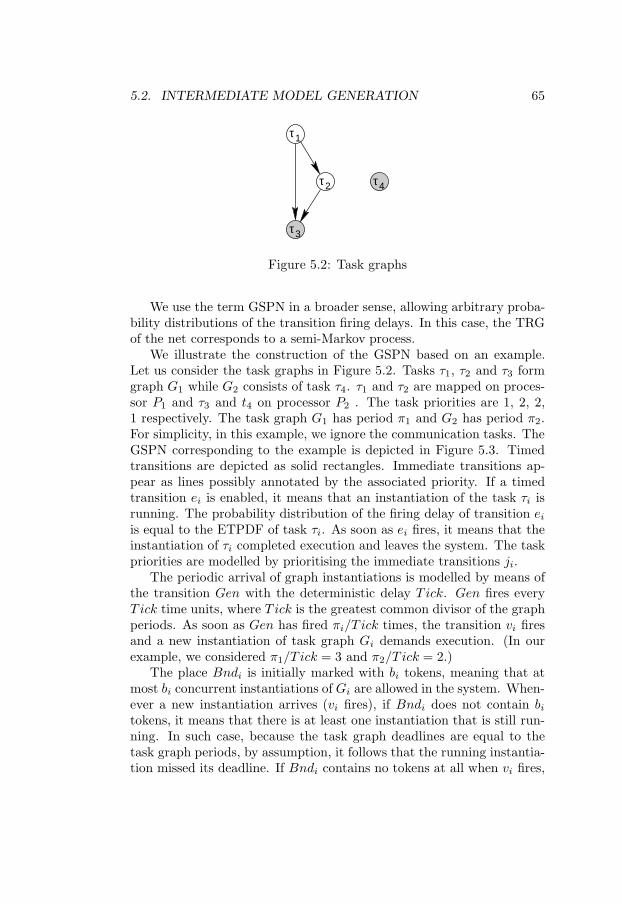
5.2. INTERMEDIATE MODEL GENERATION 65
τ1
τ2
τ3
τ4
Figure 5.2: Task graphs
We use the term GSPN in a broader sense, allowing arbitrary proba-bility distributions of the transition firing delays. In this case, the TRGof the net corresponds to a semi-Markov process.
We illustrate the construction of the GSPN based on an example.Let us consider the task graphs in Figure 5.2. Tasks τ1, τ2 and τ3 formgraph G1 while G2 consists of task τ4. τ1 and τ2 are mapped on proces-sor P1 and τ3 and t4 on processor P2 . The task priorities are 1, 2, 2,1 respectively. The task graph G1 has period π1 and G2 has period π2.For simplicity, in this example, we ignore the communication tasks. TheGSPN corresponding to the example is depicted in Figure 5.3. Timedtransitions are depicted as solid rectangles. Immediate transitions ap-pear as lines possibly annotated by the associated priority. If a timedtransition ei is enabled, it means that an instantiation of the task τi isrunning. The probability distribution of the firing delay of transition ei
is equal to the ETPDF of task τi. As soon as ei fires, it means that theinstantiation of τi completed execution and leaves the system. The taskpriorities are modelled by prioritising the immediate transitions ji.
The periodic arrival of graph instantiations is modelled by means ofthe transition Gen with the deterministic delay T ick. Gen fires everyT ick time units, where T ick is the greatest common divisor of the graphperiods. As soon as Gen has fired πi/T ick times, the transition vi firesand a new instantiation of task graph Gi demands execution. (In ourexample, we considered π1/T ick = 3 and π2/T ick = 2.)
The place Bndi is initially marked with bi tokens, meaning that atmost bi concurrent instantiations of Gi are allowed in the system. When-ever a new instantiation arrives (vi fires), if Bndi does not contain bi
tokens, it means that there is at least one instantiation that is still run-ning. In such case, because the task graph deadlines are equal to thetask graph periods, by assumption, it follows that the running instantia-tion missed its deadline. If Bndi contains no tokens at all when vi fires,
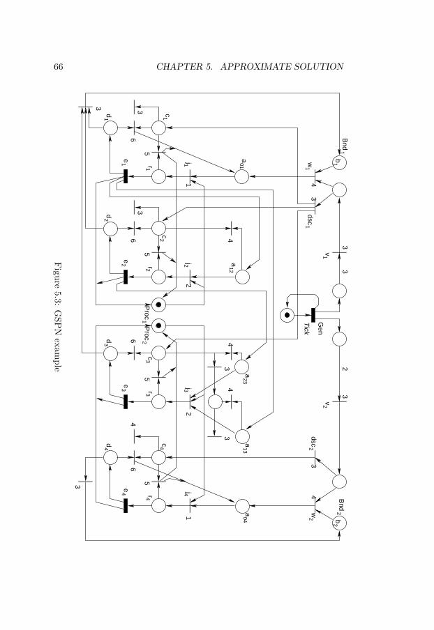
66 CHAPTER 5. APPROXIMATE SOLUTION
dsc1
dsc2
Bnd
1
a01
a13
e1
e2
Proc
1P
roc2
r3r4
12
6
5
6
5
43
43
3
6
5
4
35
63
4
3
Gen
Tick
23
33
v1
v2
w1
34
34
w2
Bnd
2b
2b
1
a12
a23
a04
1j1
2j2
j3j4
e3
e4
c1
c2
c3
c4
d3
d4
d1
d2
r1r2
Figure
5.3:G
SPN
example
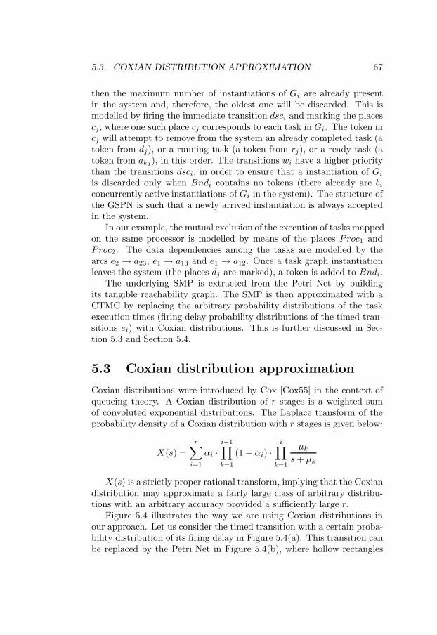
5.3. COXIAN DISTRIBUTION APPROXIMATION 67
then the maximum number of instantiations of Gi are already presentin the system and, therefore, the oldest one will be discarded. This ismodelled by firing the immediate transition dsci and marking the placescj , where one such place cj corresponds to each task in Gi. The token incj will attempt to remove from the system an already completed task (atoken from dj), or a running task (a token from rj), or a ready task (atoken from akj), in this order. The transitions wi have a higher prioritythan the transitions dsci, in order to ensure that a instantiation of Gi
is discarded only when Bndi contains no tokens (there already are bi
concurrently active instantiations of Gi in the system). The structure ofthe GSPN is such that a newly arrived instantiation is always acceptedin the system.
In our example, the mutual exclusion of the execution of tasks mappedon the same processor is modelled by means of the places Proc1 andProc2. The data dependencies among the tasks are modelled by thearcs e2 → a23, e1 → a13 and e1 → a12. Once a task graph instantiationleaves the system (the places dj are marked), a token is added to Bndi.
The underlying SMP is extracted from the Petri Net by buildingits tangible reachability graph. The SMP is then approximated with aCTMC by replacing the arbitrary probability distributions of the taskexecution times (firing delay probability distributions of the timed tran-sitions ei) with Coxian distributions. This is further discussed in Sec-tion 5.3 and Section 5.4.
5.3 Coxian distribution approximation
Coxian distributions were introduced by Cox [Cox55] in the context ofqueueing theory. A Coxian distribution of r stages is a weighted sumof convoluted exponential distributions. The Laplace transform of theprobability density of a Coxian distribution with r stages is given below:
X(s) =r∑
i=1
αi ·i−1∏k=1
(1 − αi) ·i∏
k=1
µk
s + µk
X(s) is a strictly proper rational transform, implying that the Coxiandistribution may approximate a fairly large class of arbitrary distribu-tions with an arbitrary accuracy provided a sufficiently large r.
Figure 5.4 illustrates the way we are using Coxian distributions inour approach. Let us consider the timed transition with a certain proba-bility distribution of its firing delay in Figure 5.4(a). This transition canbe replaced by the Petri Net in Figure 5.4(b), where hollow rectangles
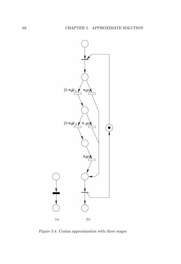
68 CHAPTER 5. APPROXIMATE SOLUTION
(a)
α1µ1(1−α1)µ1
2(1−α2)µ α2µ2
α3µ3
(b)
Figure 5.4: Coxian approximation with three stages

5.4. CTMC CONSTRUCTION AND ANALYSIS 69
represent timed transitions with exponential firing delay probability dis-tribution. The annotations near those transitions indicate their averagefiring rate. In this example, three stages have been used for approxima-tion.
Practically, the approximation problem can be formulated as follows:given an arbitrary probability distribution and a certain number of stagesr, find µi, 1 ≤ i ≤ r, and αi, 1 ≤ i ≤ r−1 (αr = 1), such that the qualityof approximation of the given distribution by the Coxian distributionwith r stages is maximised. This is usually done in the complex spaceby minimising the distance between the Fourier transform X(jω) of theCoxian distribution and the computed Fourier transform of the distri-bution to be approximated. The minimisation is a typical interpolationproblem and can be solved by various numerical methods [PTVF92].We use a simulated annealing approach that minimises the difference ofonly a few most significant harmonics of the Fourier transforms, whichis very fast if provided with a good initial solution. We choose the initialsolution in such way that the first moment of the real and approximateddistribution coincide.
By replacing all generalised transitions of the type depicted in Fig-ure 5.4(a) with subnets of the type depicted in Figure 5.4(b) the SMPunderlying the Petri Net becomes a CTMC. It is obvious that the intro-duced additional places trigger an explosion in the TRG and implicitlyin the resulted CTMC. The next section details on how to efficientlyhandle such a complexity increase.
5.4 CTMC construction and analysis
Let S be the set of states of the SMP underlying the Petri Net. ThisSMP corresponds to the TRG of the Petri Net model. Let M = [mij ]be a square matrix of size |S| × |S| where mij = 1 if there exists atransition from the state si to the state sj in the SMP and mij = 0otherwise. We first partition the set of states S in clusters such thatstates in the same cluster have outgoing edges labelled with the sameset of transitions. A cluster is identified by a binary combination thatindicates the set of transitions that are enabled in the particular cluster(equivalently, the set of tasks that are running in the states belongingto that particular cluster). The clusters are sorted according to theircorresponding binary combination and the states in the same cluster areconsecutively numbered.
Consider an example application with three independent tasks, eachof them mapped on a different processor. In this case, 8 clusters can be
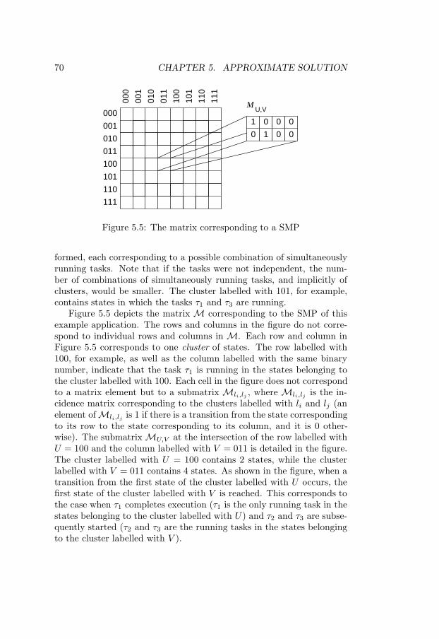
70 CHAPTER 5. APPROXIMATE SOLUTION
MU,V
000
001
010
011
100
101
110
111
111
110
101
100
011
010
001
0001 0 0
0 1 0 0
0
Figure 5.5: The matrix corresponding to a SMP
formed, each corresponding to a possible combination of simultaneouslyrunning tasks. Note that if the tasks were not independent, the num-ber of combinations of simultaneously running tasks, and implicitly ofclusters, would be smaller. The cluster labelled with 101, for example,contains states in which the tasks τ1 and τ3 are running.
Figure 5.5 depicts the matrix M corresponding to the SMP of thisexample application. The rows and columns in the figure do not corre-spond to individual rows and columns in M. Each row and column inFigure 5.5 corresponds to one cluster of states. The row labelled with100, for example, as well as the column labelled with the same binarynumber, indicate that the task τ1 is running in the states belonging tothe cluster labelled with 100. Each cell in the figure does not correspondto a matrix element but to a submatrix Mli,lj , where Mli,lj is the in-cidence matrix corresponding to the clusters labelled with li and lj (anelement of Mli,lj is 1 if there is a transition from the state correspondingto its row to the state corresponding to its column, and it is 0 other-wise). The submatrix MU,V at the intersection of the row labelled withU = 100 and the column labelled with V = 011 is detailed in the figure.The cluster labelled with U = 100 contains 2 states, while the clusterlabelled with V = 011 contains 4 states. As shown in the figure, when atransition from the first state of the cluster labelled with U occurs, thefirst state of the cluster labelled with V is reached. This corresponds tothe case when τ1 completes execution (τ1 is the only running task in thestates belonging to the cluster labelled with U) and τ2 and τ3 are subse-quently started (τ2 and τ3 are the running tasks in the states belongingto the cluster labelled with V ).
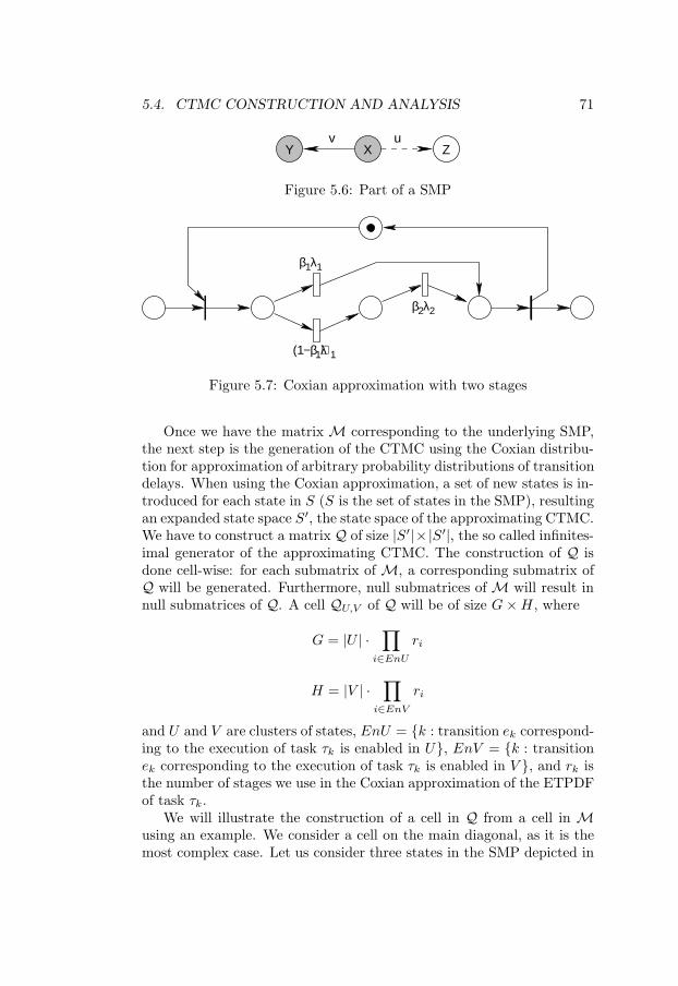
5.4. CTMC CONSTRUCTION AND ANALYSIS 71
XY Zuv
Figure 5.6: Part of a SMP
(1−β1)λ1
β1λ1
β2λ2
Figure 5.7: Coxian approximation with two stages
Once we have the matrix M corresponding to the underlying SMP,the next step is the generation of the CTMC using the Coxian distribu-tion for approximation of arbitrary probability distributions of transitiondelays. When using the Coxian approximation, a set of new states is in-troduced for each state in S (S is the set of states in the SMP), resultingan expanded state space S′, the state space of the approximating CTMC.We have to construct a matrix Q of size |S′|×|S′|, the so called infinites-imal generator of the approximating CTMC. The construction of Q isdone cell-wise: for each submatrix of M, a corresponding submatrix ofQ will be generated. Furthermore, null submatrices of M will result innull submatrices of Q. A cell QU,V of Q will be of size G × H , where
G = |U | ·∏
i∈EnU
ri
H = |V | ·∏
i∈EnV
ri
and U and V are clusters of states, EnU = k : transition ek correspond-ing to the execution of task τk is enabled in U, EnV = k : transitionek corresponding to the execution of task τk is enabled in V , and rk isthe number of stages we use in the Coxian approximation of the ETPDFof task τk.
We will illustrate the construction of a cell in Q from a cell in Musing an example. We consider a cell on the main diagonal, as it is themost complex case. Let us consider three states in the SMP depicted in

72 CHAPTER 5. APPROXIMATE SOLUTION
Y01
Y10
Y00
Y11
Y02
Y12
X01
X10
X00
X02
X11
X12
β1λ1
β1λ1
β1λ1
β2 λ2
β2 λ2
β2 λ2
α1µ1α 2µ2
α 2µ2
α1µ1
α 3µ3
α 3µ3
(1−α
1)µ 1
(1−α
1)µ 1
(1−α
1)µ 1
(1−α
1)µ 1
(1−α
2)µ 2
(1−α
2)µ 2
(1−α
2)µ 2
(1−α
2)µ 2
(1−β 1)
λ 1
(1−β 1)
λ 1
(1−β 1)
λ 1
(1−β 1)
λ 1
(1−β 1)
λ 1
(1−β 1)
λ 1
(1−α
2)µ 2
(1−α
1)µ 1
Z1
Z2
Z0
Figure 5.8: Expanded Markov chain
Figure 5.6. Two tasks, τu and τv, are running in the states X and Y .These two states belong to the same cluster, labelled with 11. Only taskτv is running in state Z. State Z belongs to cluster labelled with 10.If task τv finishes running in state X , a transition to state Y occurs inthe SMP. This corresponds to the situation when a new instantiation ofτv becomes active immediately after the completion of a previous one.When task τu finishes running in state X , a transition to state Z occursin the SMP. This corresponds to the situation when a new instantiationof τu is not immediately activated after the completion of a previous one.Consider that the probability distribution of the execution time of taskτv is approximated with the three stage Coxian distribution depicted inFigure 5.4(b) and that of τu is approximated with the two stage Coxiandistribution depicted in Figure 5.7. The resulting CTMC correspondingto the part of the SMP in Figure 5.6 is depicted in Figure 5.8. Theedges between the states are labelled with the average firing rates ofthe transitions of the Coxian distributions. Dashed edges denote statechanges in the CTMC caused by firing of transitions belonging to theCoxian approximation of the ETPDF of τu. Solid edges denote statechanges in the CTMC caused by firing of transitions belonging to the
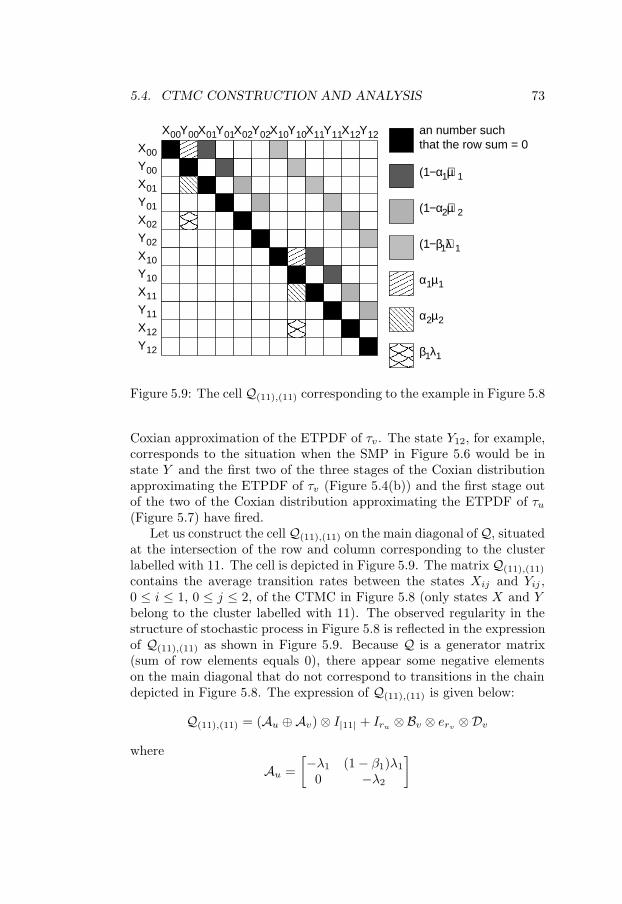
5.4. CTMC CONSTRUCTION AND ANALYSIS 73
(1−α1)µ1
(1−α2)µ2
(1−β1)λ1
α1µ1
α2µ2
β1λ1
X00 X01 X02 X10 X11 X12
X00
X01
X02
X10
X11
X12
Y00 Y01 Y02 Y10 Y11 Y12
Y00
Y01
Y02
Y10
Y11
Y12
an number suchthat the row sum = 0
Figure 5.9: The cell Q(11),(11) corresponding to the example in Figure 5.8
Coxian approximation of the ETPDF of τv. The state Y12, for example,corresponds to the situation when the SMP in Figure 5.6 would be instate Y and the first two of the three stages of the Coxian distributionapproximating the ETPDF of τv (Figure 5.4(b)) and the first stage outof the two of the Coxian distribution approximating the ETPDF of τu
(Figure 5.7) have fired.Let us construct the cell Q(11),(11) on the main diagonal of Q, situated
at the intersection of the row and column corresponding to the clusterlabelled with 11. The cell is depicted in Figure 5.9. The matrix Q(11),(11)
contains the average transition rates between the states Xij and Yij ,0 ≤ i ≤ 1, 0 ≤ j ≤ 2, of the CTMC in Figure 5.8 (only states X and Ybelong to the cluster labelled with 11). The observed regularity in thestructure of stochastic process in Figure 5.8 is reflected in the expressionof Q(11),(11) as shown in Figure 5.9. Because Q is a generator matrix(sum of row elements equals 0), there appear some negative elementson the main diagonal that do not correspond to transitions in the chaindepicted in Figure 5.8. The expression of Q(11),(11) is given below:
Q(11),(11) = (Au ⊕Av) ⊗ I|11| + Iru ⊗ Bv ⊗ erv ⊗Dv
where
Au =[−λ1 (1 − β1)λ1
0 −λ2
]
74 CHAPTER 5. APPROXIMATE SOLUTION
Bv =
α1µ1
α2µ2
α3µ3
Dv =[0 10 0
]and
Av =
−µ1 (1 − α1)µ1 0
0 −µ2 (1 − α2)µ2
0 0 −µ3
erv =[1 0 0
]|11| denotes the size of the cluster labelled with 11. Ii is the identitymatrix of size i × i, ri indicates the number of stages of the Coxiandistribution that approximates the ETPDF of task τi. ⊕ and ⊗ are theKronecker sum and product of matrices, respectively.
In general, a matrix Ak = [aij ] is an rk × rk matrix, and is definedas follows:
aij =
(1 − αki)µki if j = i + 1−µki if j = i
0 otherwise
where αki and µki characterise the ith stage of the Coxian distributionapproximating a transition tk.
A matrix Bk = [bij ] is an rk × 1 matrix and bi1 = αki ·µki. A matrixerk = [eij ] is a 1 × rk matrix and e11 = 1, e1i = 0, 1 < i ≤ rk. A matrixDk = [dij ] corresponding to a cell U, V is a |U | × |V | matrix defined asfollows:
dij =
1 if an edge labelled with k linksthe ith state of U with the jth state of V
0 otherwise
In general, considering a label U , the cell QU,U on the main diagonalof Q is obtained as follows:
QU,U =
(⊕i∈U
Ai
)⊗ I|U| +
∑i∈U
⊗
j∈Uj>i
Irj
⊗ Bi ⊗ eri ⊗
⊗
j∈Uj<i
Irj
⊗Di
A cell situated at the intersection of the row corresponding to labelU with the column corresponding to label V (U 6= V ) is obtained as
5.4. CTMC CONSTRUCTION AND ANALYSIS 75
follows:
QU,V =∑i∈U
⊗
j∈U∪V
Fij
⊗Di (5.1)
The matrices F are given by the following expression:
Fij =
vrj if j ∈ U ∧ j 6∈ V ∧ j 6= i
Irj if j ∈ U ∧ j ∈ V ∧ j 6= i
Bi if j 6∈ V ∧ j = i
Bi ⊗ eri if j ∈ V ∧ j = i
erj if j 6∈ U
(5.2)
where vrk= [vi1] is a rk × 1 matrix, vi1 = 1, 1 ≤ i ≤ rk.
The solution of the CTMC implies solving for π in the followingequation:
π · Q = 0
where π is the steady-state probability vector and Q the infinitesimalgenerator of the CTMC.
Let us consider the edge X → Z in the SMP in Figure 5.6. Theedges X00 → Z0, X10 → Z0, X01 → Z1, X11 → Z1, X02 → Z2, andX12 → Z2 in the CTMC in Figure 5.8, that approximates the SMP inFigure 5.6, correspond to the edge X → Z in the SMP. The expectedtransition rate of X → Z can be approximated by means of the expectedtransition rates of the corresponding edges in the CTMC and is givenby the expression
(πX00 + πX01 + πX02) · β1λ1 + (πX10 + πX11 + πX12 ) · β2λ2,
where β1, β2, λ1, and λ2 are characterising the Coxian distribution thatapproximates the probability distribution of the delay of the transitionX → Z (in this case, the ETPDF of τv). πXij is the probability ofthe CTMC being in state Xij after the steady state is reached. Theprobabilities πXij are obtained as the result of the numerical solution ofthe CTMC.
As explained in Section 5.2, if there already exists at least one activeinstantiation of a task graph Gi in the system when a new instantiation ofGi arrives, then the most recent instantiation of Gi present in the systemmisses its deadline (which is equal to the period). In the Petri Net model(see Figure 5.3), this event corresponds to the sequence of firings of thetimed transition Gen, followed by vi and either the immediate transitionwi if the number of tokens in Bndi is less than bi but larger than 0, or

76 CHAPTER 5. APPROXIMATE SOLUTION
the immediate transition dsci if Bndi is unmarked. Each of these twosituations corresponds to an edge in the stochastic process. Thus, theexpected deadline miss rate of Gi can be obtained by computing theexpected transition rates (as shown above for X → Z) for the edgescorresponding to a deadline miss. The expected deadline miss ratio forthe task graph Gi is then computed by multiplying the obtained expecteddeadline miss rate by the period of task graph Gi.
We conclude this section with a discussion on the size of Q and itsimplications on analysis time and memory. Consider the cluster labelled11 . . .1 of S, i.e. the one that contains the largest number of enabledtransitions. The largest Q is obtained if the cluster labelled 11 . . .1dominates all the other clusters of S, in the sense that it contains by farmore states than all the other clusters, and that the cell M(11...1),(11...1)
contains by far more non-zero entries than all the other cells of M. Thus,a pessimistic upper bound for the number of non-zero elements of Q isgiven by the expression:
|M| ·∏i∈E
ri
where E = i : transition ei corresponding to the execution of taskτi is enabled in the dominant cluster and |M| denotes the number ofnon-zero elements of M, the matrix corresponding to the SMP. In thecontext of multiprocessor scheduling, E may have at most M elements(M=number of processors). The above formula shows that the increasein the size of the CTMC, relative to the initial SMP, is mainly dictated bythe number of processors and the number of stages for the approximationof the probability distributions (which means the degree of expectedaccuracy). The number N of tasks does not directly induce any growthin terms of the CTMC. However, the structure of the initial SMP alsodepends on the number of tasks. The SMP is reflected in the matrix Mand, thus, has an influence on the dimension of the resulted CTMC.
The dimension of matrix Q, as shown above, grows quickly withthe number of processing elements and the number of stages used forapproximation of the probability distributions. Apparently, the analysisof applications of realistic complexity would be impossible. Fortunately,this is not the case. As can be seen from the expressions of QU,U andQU,V , the matrix Q is completely specified by means of the matricesAi, Bi, and Di, hence it needs not be stored explicitly in memory, butits elements are generated on-the-fly during the numerical solving of theCTMC. This leads to a significant saving in memory demand for analysis.Even for large applications, the matrices Ai, Bi, and Di are of negligiblesize. The limiting factor in terms of memory is only π, the steady-state

5.5. EXPERIMENTS 77
probability vector, which has to be stored in memory. In the worst case,the vector has
|S| ·∏i∈E
ri
elements, where |S| is the size (number of states) of the SMP. It is easyto observe that π is as large as a row (column) of Q. The effect of thecomplexity increase induced by the approximation in terms of analysistime can be attenuated by deploying intelligent numerical algorithms formatrix-vector computation. Such algorithms rely on factorisations thatexploit the particular structure of Q.
5.5 Experiments
We performed four sets of experiments. All were run on an AMD Athlonat 1533 MHz. The first set of experiments investigates the dependency ofthe analysis time on the number of tasks in the system. Sets of randomtask graphs were generated, with 9 up to 60 tasks per set. Ten differentsets were generated and analysed for each number of tasks per set. The
0
500
1000
1500
2000
2500
3000
3500
4000
4500
5000
10 20 30 40 50 60
Ana
lysi
s tim
e [s
]
Number of tasks
Individual experimentsAverage
Figure 5.10: Analysis time vs. number of tasks
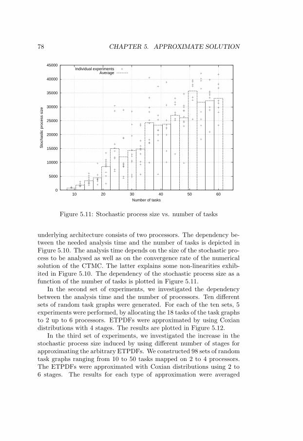
78 CHAPTER 5. APPROXIMATE SOLUTION
0
5000
10000
15000
20000
25000
30000
35000
40000
45000
10 20 30 40 50 60
Sto
chas
tic p
roce
ss s
ize
Number of tasks
Individual experimentsAverage
Figure 5.11: Stochastic process size vs. number of tasks
underlying architecture consists of two processors. The dependency be-tween the needed analysis time and the number of tasks is depicted inFigure 5.10. The analysis time depends on the size of the stochastic pro-cess to be analysed as well as on the convergence rate of the numericalsolution of the CTMC. The latter explains some non-linearities exhib-ited in Figure 5.10. The dependency of the stochastic process size as afunction of the number of tasks is plotted in Figure 5.11.
In the second set of experiments, we investigated the dependencybetween the analysis time and the number of processors. Ten differentsets of random task graphs were generated. For each of the ten sets, 5experiments were performed, by allocating the 18 tasks of the task graphsto 2 up to 6 processors. ETPDFs were approximated by using Coxiandistributions with 4 stages. The results are plotted in Figure 5.12.
In the third set of experiments, we investigated the increase in thestochastic process size induced by using different number of stages forapproximating the arbitrary ETPDFs. We constructed 98 sets of randomtask graphs ranging from 10 to 50 tasks mapped on 2 to 4 processors.The ETPDFs were approximated with Coxian distributions using 2 to6 stages. The results for each type of approximation were averaged

5.5. EXPERIMENTS 79
0
1000
2000
3000
4000
5000
6000
7000
1 2 3 4 5 6 7
Ana
lysi
s tim
e [s
]
Number of processors
Individual experimentsAverage
Figure 5.12: Analysis time vs. number of processors
over the 98 sets of graphs and the results are plotted in Figure 5.13.Recall that |S| is the size of the SMP and |S′| is the much larger size ofthe CTMC obtained after approximation. As more stages are used forapproximation, as larger the CTMC becomes compared to the originalSMP. As shown in Section 5.4, in the worst case, the growth factor is∏
i∈E
ri
As can be seen from Figure 5.13, the real growth factor is smaller than thetheoretical upper bound. It is important to emphasise that the matrixQ corresponding to the CTMC needs not to be stored, but only a vectorwith the length corresponding to a column of Q. The growth of thevector length with the number of Coxian stages used for approximationcan be easily derived from Figure 5.13. The same is the case with thegrowth of analysis time, which follows that of the CTMC.
The fourth set of experiments investigates the accuracy of resultsas a factor of the number of stages used for approximation. This isan important aspect in deciding on a proper trade-off between qualityof the analysis and cost in terms of time and memory. For compari-son, we used analysis results obtained with our approach presented in
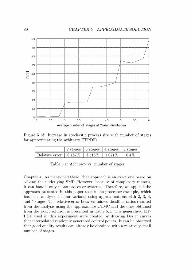
80 CHAPTER 5. APPROXIMATE SOLUTION
Average number of stages of Coxian distribution
|S/S
’|
50
100
150
200
250
300
350
400
450
500
2 2.5 3 3.5 4 4.5 5 5.5 6
Figure 5.13: Increase in stochastic process size with number of stagesfor approximating the arbitrary ETPDFs
2 stages 3 stages 4 stages 5 stagesRelative error 8.467% 3.518% 1.071% 0.4%
Table 5.1: Accuracy vs. number of stages
Chapter 4. As mentioned there, that approach is an exact one based onsolving the underlying SMP. However, because of complexity reasons,it can handle only mono-processor systems. Therefore, we applied theapproach presented in this paper to a mono-processor example, whichhas been analysed in four variants using approximations with 2, 3, 4,and 5 stages. The relative error between missed deadline ratios resultedfrom the analysis using the approximate CTMC and the ones obtainedfrom the exact solution is presented in Table 5.1. The generalised ET-PDF used in this experiment were created by drawing Bezier curvesthat interpolated randomly generated control points. It can be observedthat good quality results can already be obtained with a relatively smallnumber of stages.
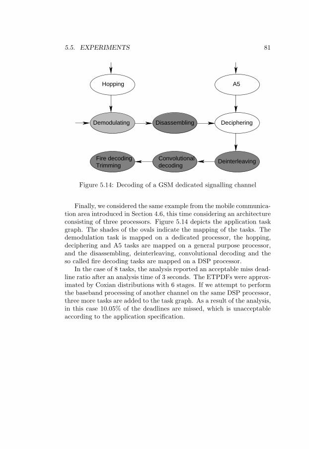
5.5. EXPERIMENTS 81
Deciphering
A5Hopping
Demodulating
Fire decodingTrimming
Disassembling
DeinterleavingConvolutionaldecoding
Figure 5.14: Decoding of a GSM dedicated signalling channel
Finally, we considered the same example from the mobile communica-tion area introduced in Section 4.6, this time considering an architectureconsisting of three processors. Figure 5.14 depicts the application taskgraph. The shades of the ovals indicate the mapping of the tasks. Thedemodulation task is mapped on a dedicated processor, the hopping,deciphering and A5 tasks are mapped on a general purpose processor,and the disassembling, deinterleaving, convolutional decoding and theso called fire decoding tasks are mapped on a DSP processor.
In the case of 8 tasks, the analysis reported an acceptable miss dead-line ratio after an analysis time of 3 seconds. The ETPDFs were approx-imated by Coxian distributions with 6 stages. If we attempt to performthe baseband processing of another channel on the same DSP processor,three more tasks are added to the task graph. As a result of the analysis,in this case 10.05% of the deadlines are missed, which is unacceptableaccording to the application specification.

82 CHAPTER 5. APPROXIMATE SOLUTION
Chapter 6
Extensions
The discussions in Chapter 4 and 5 were based on the assumptions andthe problem formulation introduced in Chapter 3. One of the main con-cerns has been to master the complexity generated by the relatively un-restricted nature of those assumptions. In this chapter, we discuss somepossible further relaxations of the assumptions introduced in Chapter 3and their consequences on the complexity of the solution.
The following extensions of the assumptions were considered:
1. The tasks belonging to the same task graph may have differentperiods.
2. The relative deadline of a task may be shorter than the task period.
3. When there are already bi concurrently active instantiations of atask graph Gi in the system at the arrival time of a new instan-tiation, instead of discarding the oldest instantiation, the newlyarrived one is rejected.
Furthermore, the problem formulation has been extended by adding theexpected deadline miss ratio per task (not only per task graph) to theoutput of the analysis. This feature provides more insight to the designerrelative to the causes of deadline misses.
Each of these extensions is treated in a separate section.
6.1 Task periods
As presented in Chapter 3, all the tasks belonging to a task graph havethe same period. This assumption has been relaxed as follows. Each
83
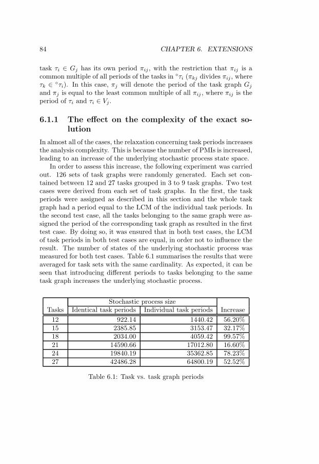
84 CHAPTER 6. EXTENSIONS
task τi ∈ Gj has its own period πij , with the restriction that πij is acommon multiple of all periods of the tasks in τi (πkj divides πij , whereτk ∈ τi). In this case, πj will denote the period of the task graph Gj
and πj is equal to the least common multiple of all πij , where πij is theperiod of τi and τi ∈ Vj .
6.1.1 The effect on the complexity of the exact so-lution
In almost all of the cases, the relaxation concerning task periods increasesthe analysis complexity. This is because the number of PMIs is increased,leading to an increase of the underlying stochastic process state space.
In order to assess this increase, the following experiment was carriedout. 126 sets of task graphs were randomly generated. Each set con-tained between 12 and 27 tasks grouped in 3 to 9 task graphs. Two testcases were derived from each set of task graphs. In the first, the taskperiods were assigned as described in this section and the whole taskgraph had a period equal to the LCM of the individual task periods. Inthe second test case, all the tasks belonging to the same graph were as-signed the period of the corresponding task graph as resulted in the firsttest case. By doing so, it was ensured that in both test cases, the LCMof task periods in both test cases are equal, in order not to influence theresult. The number of states of the underlying stochastic process wasmeasured for both test cases. Table 6.1 summarises the results that wereaveraged for task sets with the same cardinality. As expected, it can beseen that introducing different periods to tasks belonging to the sametask graph increases the underlying stochastic process.
Stochastic process sizeTasks Identical task periods Individual task periods Increase
12 922.14 1440.42 56.20%15 2385.85 3153.47 32.17%18 2034.00 4059.42 99.57%21 14590.66 17012.80 16.60%24 19840.19 35362.85 78.23%27 42486.28 64800.19 52.52%
Table 6.1: Task vs. task graph periods
6.1. TASK PERIODS 85
6.1.2 The effect on the complexity of the approxi-mate solution
Two issues have to be considered: the modifications performed on theGSPN that models the application and the impact on the analysis pro-cess.
Consider the tasks τ1, τ2 and τ3 in Figure 5.2 and let their periods beπ1 = 2, π2 = 4 and π3 = 8. τ2 executes once whenever τ1 executes twice,and τ3 executes once whenever τ1 executes four times and τ2 executestwice. This can be modelled by a GSPN similar to the one in Figure 5.3by setting the multiplicity of the arc a12 → j2 to π2/π1 (2), the one ofarc a13 → j3 to π3/π1 (4) and the one of arc a23 → j3 to π3/π2 (2).
Observe that, under the original assumptions, in the unmodifiedGSPN depicted in Figure 5.3, there is no ambiguity in the situation whena place aki is marked with more than one token. This situation wouldoccur only because of the multiple concurrently active instantiations ofa graph G. Under the extended assumptions, multiple tokens may ap-pear in a place aki because several instantiations of task τk of the sameinstantiation of G have completed, or because several instantiations oftask τk of different instantiations of G have completed. Therefore, eitherwe assume bi = 1, ∀1 ≤ i ≤ h, in the case of the extended assump-tions about task periods, or we significantly change the GSPN, whichalso increases its complexity, such that it distinguishes between tokensmodelling different graph instantiations.
In the case of discarding, under the original assumptions, at most onetoken was removed from a place aki. Under the extended assumptions,there might exist q tokens in aki, 0 ≤ q < πi/πk. Therefore, a mark-ing dependent arc multiplicity has to be introduced in order to removeexactly q tokens from aki.
If a task graph has several tasks with no predecessors and these taskshave different periods, a new scheme for modelling the task arrivals hasto be designed, which is different from that implemented with the tran-sitions v1 and v2 in Figure 5.3. Moreover, the firing delay T ick of thetimed transition Gen is given by the greatest common divisor of the taskperiods and not of the task graph periods.
The main effect of introducing individual task periods on the GSPNis an increase in the number of tokens circulating in the GSPN at a cer-tain time. This leads to a significant increase in the tangible reachabilitygraph of the GSPN and implicitly in the stochastic process size. There-fore, only small applications can be analysed under the assumption ofindividual task periods.

86 CHAPTER 6. EXTENSIONS
6.2 Deadlines shorter than periods
The restriction that the task deadlines are equal to the correspondingperiods can be relaxed too. When letting the relative deadlines of tasksto be shorter than the task periods, two conflicting effects on the analysiscomplexity are observed. On one hand, if a task misses its deadline andif the late task policy dictates that the task graph has to be discarded,fewer behaviours are possible in the interval from the discarding andthe graph deadline. This would reduce the stochastic process size. Onthe other hand, this earlier discarding introduces new contexts for thebehaviours of the rest of tasks. This would increase the stochastic processsize.
6.2.1 The effect on the complexity of the exact so-lution
In almost all of the cases, letting δi ≤ πi leads to a significant increasein the number of PMIs as seen in Figure 6.1. The considered applicationconsists of two independent tasks with periods 3 and 5 respectively.Figure 6.1(a) depicts the resulting PMIs if the relative task deadlinesare equal to the respective task periods, while Figure 6.1(b) depicts theresulting PMIs if the relative task deadlines are 2 and 4 respectively.
pmi3pmi1 pmi2 pmi4 pmi5 pmi6 pmi7τ1
τ2
0 3 5 6 9 10 12 15
(a) PMIs if δi = πi
τ1
τ2
pmi 1
pmi 2
pmi 3
pmi 4
pmi 5
pmi 6
pmi 7
pmi 11
pmi 12
pmi 8
pmi 9
pmi 10
0 3 5 6 9 152 4 8 10 11 12 14
(b) PMIs if δi ≤ πi
Figure 6.1: PMIs if deadlines are less than the periods
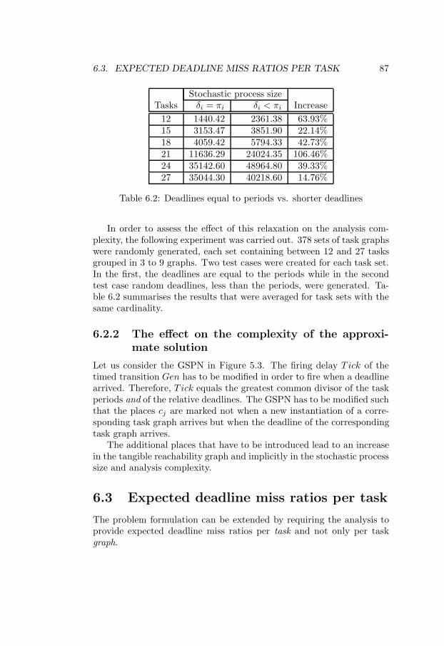
6.3. EXPECTED DEADLINE MISS RATIOS PER TASK 87
Stochastic process sizeTasks δi = πi δi < πi Increase
12 1440.42 2361.38 63.93%15 3153.47 3851.90 22.14%18 4059.42 5794.33 42.73%21 11636.29 24024.35 106.46%24 35142.60 48964.80 39.33%27 35044.30 40218.60 14.76%
Table 6.2: Deadlines equal to periods vs. shorter deadlines
In order to assess the effect of this relaxation on the analysis com-plexity, the following experiment was carried out. 378 sets of task graphswere randomly generated, each set containing between 12 and 27 tasksgrouped in 3 to 9 graphs. Two test cases were created for each task set.In the first, the deadlines are equal to the periods while in the secondtest case random deadlines, less than the periods, were generated. Ta-ble 6.2 summarises the results that were averaged for task sets with thesame cardinality.
6.2.2 The effect on the complexity of the approxi-mate solution
Let us consider the GSPN in Figure 5.3. The firing delay T ick of thetimed transition Gen has to be modified in order to fire when a deadlinearrived. Therefore, T ick equals the greatest common divisor of the taskperiods and of the relative deadlines. The GSPN has to be modified suchthat the places cj are marked not when a new instantiation of a corre-sponding task graph arrives but when the deadline of the correspondingtask graph arrives.
The additional places that have to be introduced lead to an increasein the tangible reachability graph and implicitly in the stochastic processsize and analysis complexity.
6.3 Expected deadline miss ratios per task
The problem formulation can be extended by requiring the analysis toprovide expected deadline miss ratios per task and not only per taskgraph.
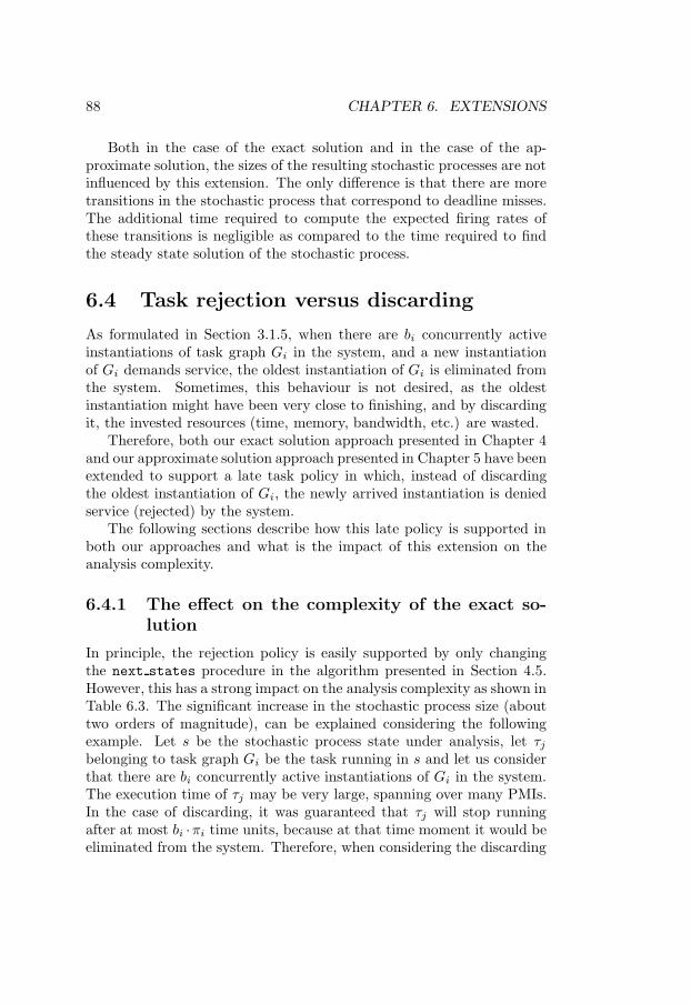
88 CHAPTER 6. EXTENSIONS
Both in the case of the exact solution and in the case of the ap-proximate solution, the sizes of the resulting stochastic processes are notinfluenced by this extension. The only difference is that there are moretransitions in the stochastic process that correspond to deadline misses.The additional time required to compute the expected firing rates ofthese transitions is negligible as compared to the time required to findthe steady state solution of the stochastic process.
6.4 Task rejection versus discarding
As formulated in Section 3.1.5, when there are bi concurrently activeinstantiations of task graph Gi in the system, and a new instantiationof Gi demands service, the oldest instantiation of Gi is eliminated fromthe system. Sometimes, this behaviour is not desired, as the oldestinstantiation might have been very close to finishing, and by discardingit, the invested resources (time, memory, bandwidth, etc.) are wasted.
Therefore, both our exact solution approach presented in Chapter 4and our approximate solution approach presented in Chapter 5 have beenextended to support a late task policy in which, instead of discardingthe oldest instantiation of Gi, the newly arrived instantiation is deniedservice (rejected) by the system.
The following sections describe how this late policy is supported inboth our approaches and what is the impact of this extension on theanalysis complexity.
6.4.1 The effect on the complexity of the exact so-lution
In principle, the rejection policy is easily supported by only changingthe next states procedure in the algorithm presented in Section 4.5.However, this has a strong impact on the analysis complexity as shown inTable 6.3. The significant increase in the stochastic process size (abouttwo orders of magnitude), can be explained considering the followingexample. Let s be the stochastic process state under analysis, let τj
belonging to task graph Gi be the task running in s and let us considerthat there are bi concurrently active instantiations of Gi in the system.The execution time of τj may be very large, spanning over many PMIs.In the case of discarding, it was guaranteed that τj will stop runningafter at most bi ·πi time units, because at that time moment it would beeliminated from the system. Therefore, when considering the discarding
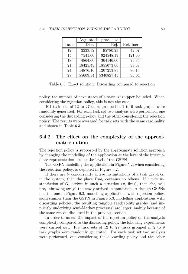
6.4. TASK REJECTION VERSUS DISCARDING 89
Avg. stoch. proc. sizeTasks Disc. Rej. Rel. incr.
12 2223.52 95780.23 42.0715 7541.00 924548.19 121.6018 4864.60 364146.60 73.8521 18425.43 1855073.00 99.6824 14876.16 1207253.83 80.1527 55609.54 5340827.45 95.04
Table 6.3: Exact solution: Discarding compared to rejection
policy, the number of next states of a state s is upper bounded. Whenconsidering the rejection policy, this is not the case.
101 task sets of 12 to 27 tasks grouped in 2 to 9 task graphs wererandomly generated. For each task set two analysis were performed, oneconsidering the discarding policy and the other considering the rejectionpolicy. The results were averaged for task sets with the same cardinalityand shown in Table 6.3.
6.4.2 The effect on the complexity of the approxi-mate solution
The rejection policy is supported by the approximate solution approachby changing the modelling of the application at the level of the interme-diate representation, i.e. at the level of the GSPN.
The GSPN modelling the application in Figure 5.2, when consideringthe rejection policy, is depicted in Figure 6.2.
If there are bi concurrently active instantiations of a task graph Gi
in the system, then the place Bndi contains no tokens. If a new in-stantiation of Gi arrives in such a situation (vi fires), then dsci willfire, “throwing away” the newly arrived instantiation. Although GSPNslike the one in Figure 6.2, modelling applications with rejection policy,seem simpler than the GSPN in Figure 5.3, modelling applications withdiscarding policies, the resulting tangible reachability graphs (and im-plicitly underlying semi-Markov processes) are larger, mainly because ofthe same reason discussed in the previous section.
In order to assess the impact of the rejection policy on the analysiscomplexity compared to the discarding policy, the following experimentswere carried out. 109 task sets of 12 to 27 tasks grouped in 2 to 9task graphs were randomly generated. For each task set two analysiswere performed, one considering the discarding policy and the other
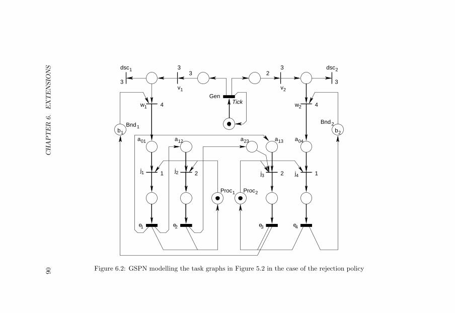
90C
HA
PT
ER
6.
EX
TE
NSIO
NS
e2 e3 e4e1
b1
Bnd1
a01
GenTick
v1 v2
j1 j2 j3 j4
dsc1 dsc2
w1 w2
b2
Bnd2
Proc1 Proc2
a12 a23 a13 a04
1 2 2 1
3
4
3
3
3
4
23
Figure 6.2: GSPN modelling the task graphs in Figure 5.2 in the case of the rejection policy
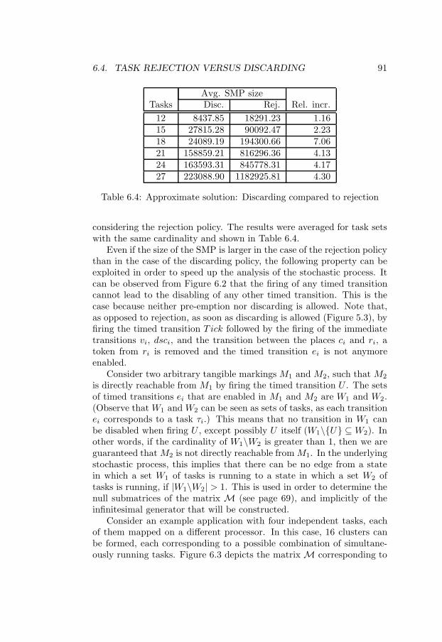
6.4. TASK REJECTION VERSUS DISCARDING 91
Avg. SMP sizeTasks Disc. Rej. Rel. incr.
12 8437.85 18291.23 1.1615 27815.28 90092.47 2.2318 24089.19 194300.66 7.0621 158859.21 816296.36 4.1324 163593.31 845778.31 4.1727 223088.90 1182925.81 4.30
Table 6.4: Approximate solution: Discarding compared to rejection
considering the rejection policy. The results were averaged for task setswith the same cardinality and shown in Table 6.4.
Even if the size of the SMP is larger in the case of the rejection policythan in the case of the discarding policy, the following property can beexploited in order to speed up the analysis of the stochastic process. Itcan be observed from Figure 6.2 that the firing of any timed transitioncannot lead to the disabling of any other timed transition. This is thecase because neither pre-emption nor discarding is allowed. Note that,as opposed to rejection, as soon as discarding is allowed (Figure 5.3), byfiring the timed transition T ick followed by the firing of the immediatetransitions vi, dsci, and the transition between the places ci and ri, atoken from ri is removed and the timed transition ei is not anymoreenabled.
Consider two arbitrary tangible markings M1 and M2, such that M2
is directly reachable from M1 by firing the timed transition U . The setsof timed transitions ei that are enabled in M1 and M2 are W1 and W2.(Observe that W1 and W2 can be seen as sets of tasks, as each transitionei corresponds to a task τi.) This means that no transition in W1 canbe disabled when firing U , except possibly U itself (W1\U ⊆ W2). Inother words, if the cardinality of W1\W2 is greater than 1, then we areguaranteed that M2 is not directly reachable from M1. In the underlyingstochastic process, this implies that there can be no edge from a statein which a set W1 of tasks is running to a state in which a set W2 oftasks is running, if |W1\W2| > 1. This is used in order to determine thenull submatrices of the matrix M (see page 69), and implicitly of theinfinitesimal generator that will be constructed.
Consider an example application with four independent tasks, eachof them mapped on a different processor. In this case, 16 clusters canbe formed, each corresponding to a possible combination of simultane-ously running tasks. Figure 6.3 depicts the matrix M corresponding to

92 CHAPTER 6. EXTENSIONS
0000
0001
0010
0011
0100
0101
0110
0111
1000
1001
1010
1011
1100
1101
1110
1111
0000
0001
0010
0011
0100
0101
0110
0111
1000
1001
1010
1011
1100
1101
1110
1111
Figure 6.3: The matrix M in the case of the rejection policy
the SMP of this example application. As in Figure 5.9, the rows andcolumns in the figure do not correspond to individual rows and columnsin M but to clusters of states. The shaded cells of M indicate thosesubmatrices that may contain non-zero elements. The blank ones arenull submatrices. For example, one such null submatrix appears at theintersection of row 1101 and column 1000. Due to the non-preemptionassumption, a task arrival or departure event may not stop the runningof another task. If the submatrix (1101, 1000) had non-zero elements itwould indicate that an event in a state where the tasks τ1, τ2, and τ4
are running, triggers a transition to a state where only the task τ1 isrunning, and two of the previously running tasks are not running any-more. This is not possible in the case of non-preemption. The submatrix(1000, 0000) may contain non-zero elements, because, if the task τ1 com-pletes execution, the stochastic process may transit to a state in whichno task is running.
Because of the property described above, the expression for com-puting a submatrix QU,V of the infinitesimal generator of the CTMC
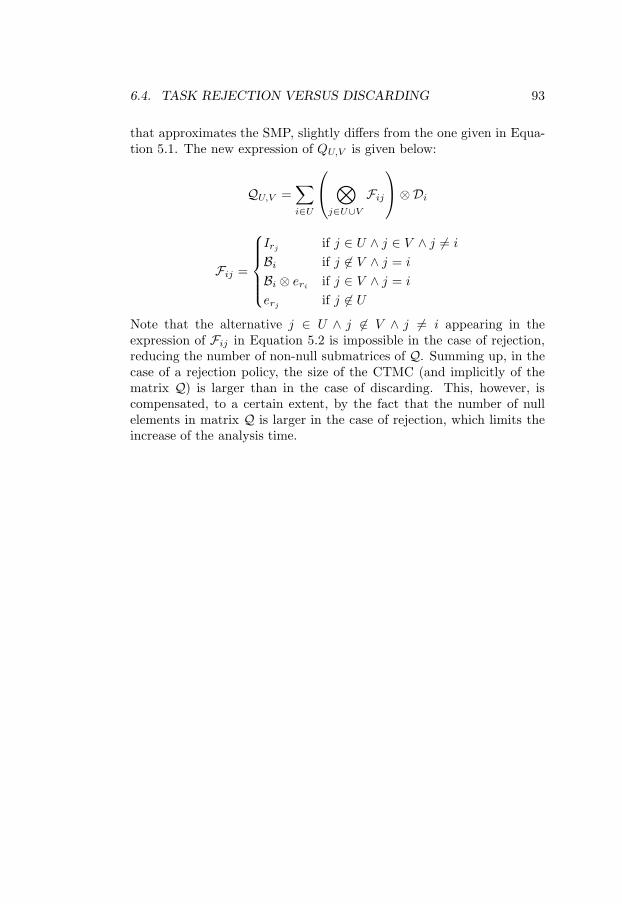
6.4. TASK REJECTION VERSUS DISCARDING 93
that approximates the SMP, slightly differs from the one given in Equa-tion 5.1. The new expression of QU,V is given below:
QU,V =∑i∈U
⊗
j∈U∪V
Fij
⊗Di
Fij =
Irj if j ∈ U ∧ j ∈ V ∧ j 6= i
Bi if j 6∈ V ∧ j = i
Bi ⊗ eri if j ∈ V ∧ j = i
erj if j 6∈ U
Note that the alternative j ∈ U ∧ j 6∈ V ∧ j 6= i appearing in theexpression of Fij in Equation 5.2 is impossible in the case of rejection,reducing the number of non-null submatrices of Q. Summing up, in thecase of a rejection policy, the size of the CTMC (and implicitly of thematrix Q) is larger than in the case of discarding. This, however, iscompensated, to a certain extent, by the fact that the number of nullelements in matrix Q is larger in the case of rejection, which limits theincrease of the analysis time.

94 CHAPTER 6. EXTENSIONS

Chapter 7
Conclusions and FutureWork
7.1 Conclusions
The design process of real-time embedded systems is an extremely com-plex task, requiring a disciplined and systematic methodology as wellas the support of design space exploration and performance estimationtools.
It is of capital importance that the predicted performance of a notyet implemented system is an accurate estimate of the performance tobe achieved by the implemented system. In order to obtain such accu-rate results and still not commit to an implementation, the performanceestimation tool has to be fed with an architecture alternative, a mappingalternative, and a scheduling alternative.
This thesis presented two approaches for the performance estima-tion of real-time systems with stochastic execution times in the contextmentioned above.
The first approach delivers exact results and it is applicable, buttheoretically not limited, to mono-processor systems. In this case, ap-plications under a fairly relaxed set of assumptions are considered. Theinnovative way of concurrently constructing and analysing the stochas-tic process underlying the application, as well as the economic methodof parsing the stochastic process allows for the consideration of larger,real-world applications.
The second approach may trade result accuracy for analysis resources(time and memory space) and it is applicable to multi-processor systems
95
96 CHAPTER 7. CONCLUSIONS AND FUTURE WORK
as well. It relies on a designer controlled approximation of real-worldexecution time probability distribution functions by means of Coxiandistributions and on the efficient way of solving the resulting Markovchain without the need to explicitly store the generator matrix.
Experiments were carried out for both approaches in order to assesstheir applicability.
7.2 Future work
Future work could focus on three possible directions:
1. Better support for design space exploration,
2. More efficient extraction of the performance indicators,
3. Extending the assumptions regarding the applications amenable toanalysis.
Along the first line, further performance indicators, besides the ex-pected deadline miss ratios, have to be found, such that they bettersupport the design exploration phase. Such information could be usefulfor deciding on different scheduling policies, task mappings and architec-tures. If significantly different implementations of the same applicationneed to be compared, the accuracy of the results is not very important.Rather, the results should provide crude guidelines for further explo-ration of one of the evaluated implementation. Therefore, the trade-offanalysis complexity versus result accuracy has to be further investigatedin more detail.
Along the second line, symmetries at the application level, as wellas at the intermediate representation level, could be exploited in orderto further reduce the analysis complexity and still obtain the desiredperformance indicators of interest.
Along the third line, the class of applications amenable to analysiscould encompass applications with shared resources, and applicationswhere the task mapping is not unique, but rather a set of alternativemappings is concurrently evaluated.
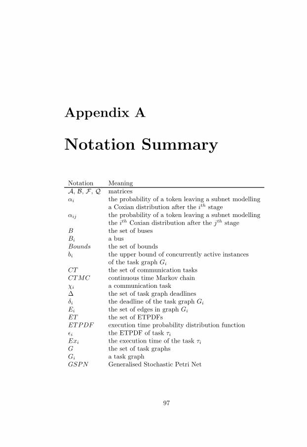
Appendix A
Notation Summary
Notation MeaningA, B, F , Q matricesαi the probability of a token leaving a subnet modelling
a Coxian distribution after the ith stageαij the probability of a token leaving a subnet modelling
the ith Coxian distribution after the jth stageB the set of busesBi a busBounds the set of boundsbi the upper bound of concurrently active instances
of the task graph Gi
CT the set of communication tasksCTMC continuous time Markov chainχi a communication task∆ the set of task graph deadlinesδi the deadline of the task graph Gi
Ei the set of edges in graph Gi
ET the set of ETPDFsETPDF execution time probability distribution functionεi the ETPDF of task τi
Exi the execution time of the task τi
G the set of task graphsGi a task graphGSPN Generalised Stochastic Petri Net
97
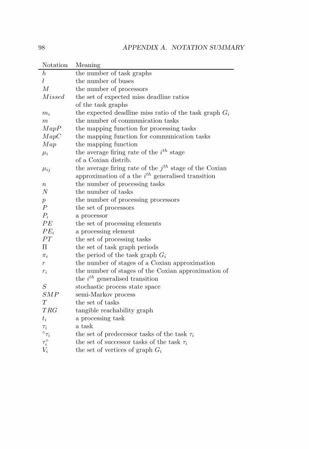
98 APPENDIX A. NOTATION SUMMARY
Notation Meaningh the number of task graphsl the number of busesM the number of processorsMissed the set of expected miss deadline ratios
of the task graphsmi the expected deadline miss ratio of the task graph Gi
m the number of communication tasksMapP the mapping function for processing tasksMapC the mapping function for communication tasksMap the mapping functionµi the average firing rate of the ith stage
of a Coxian distrib.µij the average firing rate of the jth stage of the Coxian
approximation of a the ith generalised transitionn the number of processing tasksN the number of tasksp the number of processing processorsP the set of processorsPi a processorPE the set of processing elementsPEi a processing elementPT the set of processing tasksΠ the set of task graph periodsπi the period of the task graph Gi
r the number of stages of a Coxian approximationri the number of stages of the Coxian approximation of
the ith generalised transitionS stochastic process state spaceSMP semi-Markov processT the set of tasksTRG tangible reachability graphti a processing taskτi a taskτi the set of predecessor tasks of the task τi
τi the set of successor tasks of the task τi
Vi the set of vertices of graph Gi
Appendix B
Elements of ProbabilityTheory and StochasticProcesses
Definition 1 Let Ω be a set and F ⊆ 2Ω. F is a σ-algebra if
1. ∅ ∈ F2. A ∈ F ⇒ A ∈ F3. ∀i ∈ I ⊆ N, Ai ∈ F , Ai ⊆ Aj , ∀i < j ⇒ ⋃
i∈I Ai ∈ F
Definition 2 The tuple (Ω,F) is a measurable space if F is a σ-algebra.
Definition 3 A set function λ : F → R is countably additive if Ai ∈F , i ∈ I ⊆ N, Ak ∩ Al = ∅, ∀k, l ∈ I, k 6= l,⇒ λ(
⋃i∈I Ai) =
∑i∈I λ(Ai).
Definition 4 The countably additive set function P : F → R is a prob-ability measure if it is positively defined, (Ω,F) is a measurable spaceand P(Ω) = 1.
Definition 5 The tuple (Ω,F , P) is a probability space if (Ω,F) is ameasurable space and P is a probability measure defined on F .
Definition 6 Let (Ω,F) and (S,S) be two measurable spaces and X :Ω → S. If ∀A ∈ S, ω : X(ω) ∈ A ∈ F then X is a measurable function
99
100 APPENDIX B. ELEMENTS OF PROBABILITY THEORY
Definition 7 Let (Ω,F , P) be a probability space, (S,S) a measurablespace and X : Ω → S a measurable function. Then X is a randomvariable.
Definition 8 Let (Ω,F , P) be a probability space, (S,S) a measurablespace and X : Ω → S a random variable. The probability measureP : S → R, P (A) = P(X−1A) = Pω : X(ω) ∈ A, ∀A ∈ S is thedistribution of X.
Theorem 1 Let (R,B) be a real measurable space, where B is a Borel al-gebra, i.e. the σ-algebra of open sets (open intervals in this case). For ev-ery monotone increasing right-continuous real function F : R → R withlimt→∞ F (t) = 1, there exists a unique probability measure PF which isthe extension on Borel sets of the unique measure function P∗
F ((a, b]) =F (b) − F (a). Conversely, for every probability measure P on (R,B)there exists a unique monotone increasing right-continuous real functionFP : R → R, limt→∞ F (t) = 1 such that FP(b) − FP(a) = P((a, b]).
Definition 9 Let (Ω,F , P) be a probability space, (R,B) a real measur-able space, where B are the Borel sets of the line, let X : Ω → R be arandom variable and let F : R → R be the monotone increasing right-continuous real function corresponding to the distribution of X. If Fis continuous, then X is a continuous random variable. Conversely, if∑
t∈D F (t) = 1, where D is the set of discontinuity points of F , then Xis a discrete random variable.
Definition 10 Let (Ω,F , P) be a probability space. The set Xt : t ∈ Iof random variables with values in some arbitrary real measurable space(S,S), set is a stochastic process. If I is discrete, then Xt is a discretetime stochastic process. Otherwise, Xt is a continuous time stochasticprocess. If S is finite, the stochastic process is a discrete state stochasticprocess or a chain.
Definition 11 Let (Ω,F , P) be a probability space and the family ofrandom variables on Ω Xt : t ∈ I be a stochastic process. xω : I → R,xω(t) = Xt(ω) is a sample path or a sample function of the stochasticprocess.
Definition 12 Let Xt : t ∈ I be a stochastic process. The intervalsduring which the sample paths are constant are called the state holdingtimes.
Definition 13 Let Xt : t ∈ I ⊆ R be a stochastic process with statespace S. If P(Xt+u = j|Xt = i, Xs, 0 ≤ s < t, u > 0) = P(Xt+u =
101
j|Xt = i, u > 0), ∀t ∈ I, ∀i, j ∈ S, ∀u > 0, then the process exhibits theMarkovian property and is a Markov process.
Definition 14 Let F : [0,∞) → R be the distribution of a real valuedrandom variable X. If F is of the form F (t) = 1 − e−λt then X isexponentially distributed or is an exponential random variable.
Definition 15 Let X be a real valued random variable and let P be itsdistribution. If P(X ≤ x+u|X > x) = P(X ≤ u), then P is a memorylessdistribution.
Theorem 2 The exponential distributions are the only continuous mem-oryless distributions.
Theorem 3 A Markovian continuous time stochastic process has expo-nentially distributed state holding times.
Definition 16 Let Xt : t ∈ I be a continuous time stochastic process.Let t1 < t2 < · · · < tk < . . . be the points where the process changes stateand let I ′ be their set. If the discrete time stochastic process Xn : tn ∈I ′ is Markovian, then Xt is a semi-Markov process and the Xn isits embedded Markov process.
102 APPENDIX B. ELEMENTS OF PROBABILITY THEORY
Bibliography
[AB98] A. Atlas and A. Bestavros. Statistical rate monotonicscheduling. In Proceedings of the 19th IEEE Real-Time Sys-tems Symposium, pages 123–132, 1998.
[AB99] L. Abeni and G. Butazzo. QoS guarantee using probabilisticdeadlines. In Proceedings of the 11th Euromicro Conferenceon Real-Time Systems, pages 242–249, 1999.
[ABD+91] N. C. Audsley, A. Burns, R. I. Davis, K. W. Tindell, andA. J. Wellings. Hard real-time scheduling: The deadlinemonotonic approach. In Proceedings of the 8th IEEE Work-shop on Real-Time Operating Systems and Software, pages133–137, 1991.
[ABR+93] N. Audsley, A. Burns, M. Richardson, K. Tindell, andA. Wellings. Applying new scheduling theory to static pri-ority pre-emptive scheduling. Software Engineering Journal,8(5):284–292, 1993.
[ABRW93] N. C Audsley, A. Burns, M. F. Richardson, and A. J.Wellings. Incorporating unbounded algorithms into pre-dictable real-time systems. Computer Systems Science andEngineering, 8(3):80–89, 1993.
[ACZD94] G. Agrawal, B. Chen, W. Zhao, and S. Davari. Guaran-teeing synchronous message deadlines with the timed to-ken medium access control protocol. IEEE Transactions onComputers, 43(3), March 1994.
[Aud91] N. C. Audsley. Optimal priority assignment and feasibility ofstatic priority tasks with arbitrary start times. Technical Re-port YCS 164, Department of Computer Science, Universityof York, December 1991.
103

104 BIBLIOGRAPHY
[BBB01] E. Bini, G. Butazzo, and G. Butazzo. A hyperbolic boundfor the rate monotonic algorithm. In Proceedings of the 13th
Euromicro Conference on Real-Time Systems, pages 59–66,2001.
[BCFR87] G. Balbo, G. Chiola, G. Franceschinis, and G. M. Roet. Onthe efficient construction of the tangible reachability graphof generalized stochastic petri nets. In Proceedings of the 2nd
Workshop on Petri Nets and Performance Models, pages 85–92, 1987.
[Bla76] J. Blazewicz. Scheduling dependent tasks with different ar-rival times to meet deadlines. In E. Gelenbe and H. Bellner,editors, Modeling and Performance Evaluation of ComputerSystems. North-Holland, Amsterdam, 1976.
[BRH90] S. K. Baruah, L. E. Rosier, and R. R Howell. Algorithms andcomplexity concerning the preemptive scheduling of periodic,real-time tasks on one processor. Journal of Real-Time Sys-tems, 2(4):301–324, 1990.
[Bur79] D. Y. Burman. An Analytic Approach to Diffusion Approx-imation in Queueing. PhD thesis, New York University,February 1979.
[But97] Giorgio C. Butazzo. Hard Real-Time Computing Systems.Kluwer Academic, 1997.
[BW94] A. Burns and A. Wellings. Real-Time Systems and TheirProgramming Languages. Addison Wesley, 1994.
[Cox55] D. R. Cox. A use of complex probabilities in the theory ofstochastic processes. In Proceedings of the Cambridge Philo-sophical Society, pages 313–319, 1955.
[CSB90] H. Chetto, M. Silly, and T. Bouchentouf. Dynamic schedul-ing of real-time tasks under precedence constraints. Journalof Real-Time Systems, 2:325–346, 1990.
[DF01] R. Dobrin and G. Fohler. Implementing off-line messagescheduling on Controller Area Network (CAN). In Proceed-ings of the 8th IEEE International Conference on EmergingTechnologies and Factory Automation, volume 1, pages 241–245, 2001.
BIBLIOGRAPHY 105
[dJG00] G. de Veciana, M. Jacome, and J.-H. Guo. Assessing proba-bilistic timing constraints on system performance. DesignAutomation for Embedded Systems, 5(1):61–81, February2000.
[DLS01] B. Doytchinov, J. P. Lehoczky, and S. Shreve. Real-timequeues in heavy traffic with earliest-deadline-first queue dis-cipline. Annals of Applied Probability, 11:332–378, 2001.
[Doo94] J.L. Doob. Measure Theory. Springer, 1994.
[DW93] J. G. Dai and Y. Wang. Nonexistence of Brownian modelsfor certain multiclass queueing networks. Queueing Systems,13:41–46, 1993.
[EDPP00] P. Eles, A. Doboli, P. Pop, and Z. Peng. Scheduling withbus access optimization for distributed embedded systems.IEEE Transactions on Very Large Scale Integrated (VLSI)Systems, 8(5):472–491, October 2000.
[EHS97] H. Ermedahl, H. Hansson, and M. Sjodin. Response-timeguarantees in ATM networks. In Proceedings of the Real-Time Systems Symposium, pages 274–284, 1997.
[Ele02] P. Eles. System design and methodology, 2002.http://www.ida.liu.se/˜TDTS30/.
[Ern98] R. Ernst. Codesign of embedded systems: Status and trends.IEEE Design and Test of Computers, pages 45–54, April-June 1998.
[FJ98] M. Frigo and S. G. Johnson. FFTW: An adaptive softwarearchitecture for the FFT. In Proceedings of the IEEE Inter-national Conference on Acoustics, Speech and Signal Pro-cessing, volume 3, pages 1381–1384, 1998.
[GI99] A. Goel and P. Indyk. Stochastic load balancing and relatedproblems. In IEEE Symposium on Foundations of ComputerScience, pages 579–586, 1999.
[GJ75] M. R. Garey and D. S. Johnson. Complexity results formultiprocessor scheduling under resource constraints. SIAMJournal on Computing, 4(4):397–411, 1975.
[GJ79] M. R. Garey and D. S. Johnson. Computers and Intractabil-ity. Freeman, 1979.
106 BIBLIOGRAPHY
[GKL91] M. Gonzalez Harbour, M. H. Klein, and J. P. Lehoczky.Fixed priority scheduling of periodic rasks with varying ex-ecution priority. In Proceedings of the IEEE Real Time Sys-tems Symposium, pages 116–128, 1991.
[GKL94] M. Gonzalez Harbour, M. H. Klein, and J. P. Lehoczky.Timing analysis for fixed-priority scheduling of hard real-time systems. IEEE Transactions on Software Engineering,20(1):13–28, January 1994.
[HN93] J. M. Harrison and V. Nguyen. Brownian models of multi-class queueing networks: Current status and open problems.Queueing Systems, 13:5–40, 1993.
[HST97] H. Hansson, M. Sjodin, and K. Tindell. Guaranteeing real-time traffic through an ATM network. In Proceedings of the30th Hawaii International Conference on System Sciences,volume 5, pages 44–53, 1997.
[HZS01] X. S. Hu, T. Zhou, and E. H.-M. Sha. Estimating proba-bilistic timing performance for real-time embedded systems.IEEE Transactions on Very Large Scale Integration (VLSI)Systems, 9(6):833–844, December 2001.
[JMEP00] R. Jigorea, S. Manolache, P. Eles, and Z. Peng. Modellingof real-time embedded systems in an object oriented designenvironment with UML. In Proceedings of the 3rd IEEE In-ternational Symposium on Object-Oriented Real-Time Dis-tributed Computing (ISORC00), pages 210–213, March 2000.
[JP86] M. Joseph and P. Pandya. Finding response times in a real-time system. The Computer Journal, 29(5):390–395, 1986.
[KFG+92] H. Kopetz, G. Fohler, G. Grunsteidl, H. Kantz, G. Pospis-chil, P. Puschner, J. Reisinger, R. Schlatterbeck, W. Schutz,A. Vrchoticky, and R. Zainlinger. The programmer’s viewof MARS. In Proceedings of the Real-Time Systems Sympo-sium, pages 223–226, 1992.
[KM98] A. Kalavade and P. Moghe. A tool for performance esti-mation of networked embedded end-systems. In Proceedingsof the 35th Design Automation Conference, pages 257–262,1998.
[Kop97] H. Kopetz. Real-Time Systems. Kluwer Academic, 1997.
BIBLIOGRAPHY 107
[KRT00] J. Kleinberg, Y. Rabani, and E. Tardos. Allocating band-width for bursty connections. SIAM Journal on Computing,30(1):191–217, 2000.
[KS96] J. Kim and K. G. Shin. Execution time analysis of commu-nicating tasks in distributed systems. IEEE Transactions onComputers, 45(5):572–579, May 1996.
[KS97] C. M. Krishna and K. G. Shin. Real-Time Systems. McGraw-Hill, 1997.
[Leh96] J. P. Lehoczky. Real-time queueing theory. In Proceedingsof the 18th Real-Time Systems Symposium, pages 186–195,December 1996.
[Leh97] J. P. Lehoczky. Real-time queueing network theory. In Pro-ceedings of the 19th Real-Time Systems Symposium, pages58–67, December 1997.
[LL73] C. L. Liu and J. W. Layland. Scheduling algorithms formultiprogramming in a hard-real-time environment. Journalof the ACM, 20(1):47–61, January 1973.
[LSD89] J. Lehoczky, L. Sha, and Y. Ding. The rate monotonicscheduling algorithm: Exact characterization and averagecase behaviour. In Proceedings of the 11th Real-Time Sys-tems Symposium, pages 166–171, 1989.
[LW82] J. Y. T. Leung and J. Whitehead. On the complexity of fixed-priority scheduling of periodic, real-time tasks. PerformanceEvaluation, 2(4):237–250, 1982.
[MA95] Y. Manabe and S. Aoyagi. A feasibility decision algorithm forrate monotonic scheduling of real-time tasks. In Proceedingsof the Real-Time Technology and Applications Symposium,pages 212–218, 1995.
[MEP01] S. Manolache, P. Eles, and Z. Peng. Memory and time-efficient schedulability analysis of task sets with stochasticexecution time. In Proceedings of the 13th Euromicro Con-ference on Real Time Systems, pages 19–26, June 2001.
[MEP02] S. Manolache, P. Eles, and Z. Peng. Schedulability analysisof multiprocessor real-time applications with stochastic taskexecution times. In Proceedings of the 20th InternationalConference on Computer Aided Design, November 2002.

108 BIBLIOGRAPHY
[PEP99] P. Pop, P. Eles, and Z. Peng. Scheduling with optimizedcommunication for time-triggered embedded systems. InProceedings of the 7th International Workshop on Hardware-Software Co-Design, pages 178–182, May 1999.
[PEP00] P. Pop, P. Eles, and Z. Peng. Bus access optimization fordistributed embedded systems based on schedulability anal-ysis. In Proceedings of Conference on Design, Automationand Test in Europe, pages 567–575, 2000.
[PEP02] T. Pop, P. Eles, and Z. Peng. Holistic scheduling and analy-sis of mixed time/event triggered distributed embedded sys-tems. In Proceedings of the 10th International Symposium onHardware-Software Co-Design, pages 187–192, May 2002.
[PG98] J. C. Palencia Gutierrez and M. Gonzalez Harbour. Schedu-lability analysis for tasks with static and dynamic offsets.In Proceedings of the 19th IEEE Real Time Systems Sympo-sium, pages 26–37, December 1998.
[PKH01] E. L. Plambeck, S. Kumar, and J. M. Harrison. A multi-class queue in heavy traffic with throughput time constraints:Asymptotically optimal dynamic controls. Queueing Sys-tems, 39(1):23–54, September 2001.
[Ple92] P. Pleinevaux. An improved hard real-time scheduling forthe IEEE 802.5. Journal of Real-Time Systems, 4(2):99–112,1992.
[PTVF92] W. H. Press, S. A. Teukolsky, W. T. Vetterling, and B. P.Flannery. Numerical Recipes in C. Cambridge UniversityPress, 1992.
[SGL97] J. Sun, M. K. Gardner, and J. W. S. Liu. Bounding com-pletion times of jobs with arbitrary release times, variableexecution times, and resource sharing. IEEE Transactionson Software Engineering, 23(10):604–615, October 1997.
[SL95] J. Sun and J. W. S. Liu. Bounding the end-to-end responsetime in multiprocessor real-time systems. In Proceedings ofthe Workshop on Parallel and Distributed Real-Time Sys-tems, pages 91–98, April 1995.
[SM89] J. K. Strosnider and T. E. Marchok. Responsive, determinis-tic IEEE 802.5 token ring scheduling. Journal of Real-TimeSystems, 1(2):133–158, 1989.

BIBLIOGRAPHY 109
[Spu96a] M. Spuri. Analysis of deadline scheduled real-time systems.Technical Report 2772, INRIA Rocquencourt, Le ChesnayCedex, France, January 1996.
[Spu96b] M. Spuri. Holistic analysis for deadline scheduled real-timedistributed systems. Technical Report 2873, INRIA Roc-quencourt, Le Chesnay Cedex, France, April 1996.
[SS94] M. Spuri and J. A. Stankovic. How to integrate prece-dence constraints and shared resources in real-time schedul-ing. IEEE Transactions on Computers, 43(12):1407–1412,December 1994.
[SSDB94] J. A. Stankovic, M. Spuri, M. Di Natale, and G. C. Butazzo.Implications of classical scheduling results for real-time sys-tems. Technical Report UM-CS-94-089, Computer ScienceDepartment, University of Massachusetts, 1994.
[Sun97] J. Sun. Fixed-Priority End-to-End Scheduling in DistributedReal-Time Systems. PhD thesis, University of Illinois atUrbana-Champaign, 1997.
[TC94] K. Tindell and J. Clark. Holistic schedulability analysis fordistributed real-time systems. Euromicro Jurnal on Micro-processing and Microprogramming (Special Issue on ParallelEmbedded Real-Time Systems), 40:117–134, 1994.
[TDS+95] T.-S. Tia, Z. Deng, M. Shankar, M. Storch, J. Sun, L.-C.Wu, and J. W. S. Liu. Probabilistic performance guaranteefor real-time tasks with varying computation times. In Pro-ceedings of the IEEE Real-Time Technology and ApplicationsSymposium, pages 164–173, May 1995.
[THW94] K. W. Tindell, H. Hansson, and A. J. Wellings. Analysingreal-time communications: Controller Area Network (CAN).In Proceedings of the Real-Time Systems Symposium, pages259–263, 1994.
[Tin94] K. Tindell. Adding time-offsets to schedulability analysis.Technical Report YCS 221, Department of Computer Sci-ence, University of York, January 1994.
[Ull75] J. D. Ullman. NP-complete scheduling problems. Journal ofComputer and System Sciences, 10(3):384–393, June 1975.
110 BIBLIOGRAPHY
[Wil98] R. J. Williams. Diffusion approximations for open multi-class queueing networks: Sufficient conditions involving statespace collapse. Queueing Systems, 30:27–88, 1998.
[ZHS99] T. Zhou, X. (S.) Hu, and E. H.-M. Sha. A probabilistic per-formace metric for real-time system design. In Proceedings ofthe 7th International Workshop on Hardware-Software Co-Design, pages 90–94, 1999.