Scenery reconstruction in two dimensions with manycolorsLöwe, M.; Matzinger, H.

Published: 01/01/1999

Document VersionPublisher’s PDF, also known as Version of Record (includes final page, issue and volume numbers)

Please check the document version of this publication:

• A submitted manuscript is the author's version of the article upon submission and before peer-review. There can be important differencesbetween the submitted version and the official published version of record. People interested in the research are advised to contact theauthor for the final version of the publication, or visit the DOI to the publisher's website.• The final author version and the galley proof are versions of the publication after peer review.• The final published version features the final layout of the paper including the volume, issue and page numbers.

Link to publication

Citation for published version (APA):Löwe, M., & Matzinger, H. (1999). Scenery reconstruction in two dimensions with many colors. (ReportEurandom; Vol. 99018). Eindhoven: Eurandom.

General rightsCopyright and moral rights for the publications made accessible in the public portal are retained by the authors and/or other copyright ownersand it is a condition of accessing publications that users recognise and abide by the legal requirements associated with these rights.

• Users may download and print one copy of any publication from the public portal for the purpose of private study or research. • You may not further distribute the material or use it for any profit-making activity or commercial gain • You may freely distribute the URL identifying the publication in the public portal ?

Take down policyIf you believe that this document breaches copyright please contact us providing details, and we will remove access to the work immediatelyand investigate your claim.

Download date: 11. Jun. 2018

Report 99-018 Scenery Reconstruction in Two Dimensions

with many Colors Matthias Lowe

Heinrich Matzinger III ISSN: 1389-2355

SCENERY RECONSTRUCTION IN TWO DIMENSIONS

WITH MANY COLORS

MATTHIAS LOWE AND HEINRICH MATZINGER III

ABSTRACT. In [6) Kesten observed that the known reconstruction methods of random sceneries seem to strongly depend on the one dimensional setting of the problem and asked whether a construction still is possible in two dimensions. In this paper we answer the above question in the affirmative under the condition that the number of colors in the scenery is large enough.

1. INTRODUCTION AND THE MAIN RESULT

The following problem has its roots in ergodic theory but may also be considered interesting in its own rights. Consider a graph (V, E) and color its vertices in an arbitrary way (so we do not only concentrate on proper colorings in the strict sense that any two adjacent vertices need to have a different color). This coloring will be called a scenery on (V, E). Then we run a random walk on (V, E) of which we only know the color record (i.e. the sequence of colors it reads at the vertices) but not where it actually reads them. The question then is: Can we still say anything about how V was colored?

This problem - which at first glance might seem a bit hopeless - was first investi­gated independently by Benjamini and den Hollander and Keane [5]. From here the problem splits into basically three branches:

1. Can we distinguish two (known) sceneries by their random walk record? or, more ambitiously:

2. Can we even reconstruct (unknown) sceneries by the observations we obtain from a random walk? and:

3. Are their sceneries which cannot be reconstructed or distinguished by the color record of a random walk?

Basic answers to all of these three question have been already given while other aspects are still wide open. For example Benjamini and Kesten [1] discovered the very strong result that almost surely any two given sceneries on the integer lattices Z or Z2 can be distinguished by a simple random walk on these lattices given that the colors are selected by an LLd. process. Matzinger [9] showed that on Z even more is true: Almost every i.i.d. two-color scenery can be reconstructed from the color record of a simple random walk (which even might have non zero probability to stand still). This implies Benjamini's and Kesten's result in one dimension as well as the earlier observation by the same author that the same holds true for three and more colors [8]. However, notice that Benjamini's and Kesten's techniques also work in a two dimensional situation or when the random walk is allowed to jump.

Date: May 12, 1999. 1991 Mathematics Subject Classification. 28A99, 60J15 (primary). Key words and phrases. Scenery, Random walk, Coloring.

1

2 M. LOWE AND H. MATZINGER

A remarkable answer to Question 3 has been given by Lindenstrauss [7] who showed that there are still uncountably many sceneries on Z which cannot be distinguished from the color record of a simple random walk.

To be more specific: In what follows (V, E) will always be the integer lattice Z2 and a function ~ : Z2 ---* Z will be called a two dimensional scenery. For a subset D c Z2 we call ~ : D ---* Z a piece of scenery. If the range of ~ contains exactly m elements we will say that ~ has m colors or that it is an m-color scenery. Two sceneries ~ and ~ will be called equivalent, if there are a E Z2 and

M E { (~1 ~) , (~ ~1)' (~1 ~1)' (~ ~)} such that

~(x) = ~(Mx + a)

Similarly, we call two pieces of scenery ~ : D ---* Z and ~ : D --+ Z equivalent, if again

~(x) = ~(Mx + a) Vx E D

holds true (a and M as above) and moreover M(D) + a = D. In other words ~ and ~ are equivalent (in symbols ~ f'V ~) if they can be obtained by translation and reflection on the coordinate axes from each other. It is rather obvious that in general we cannot expect to distinguish equivalent sceneries by their color record and thus also reconstruction will work only up to equivalence. Throughout this paper we will consider ~'s that result from an unbiased ij.d. random process with m colors (thus we will also say that ~ has m colors), that is the ~(v) are Li.d. for all v E Z2 and

1 P(~(O) = i) = -

m for all colors i E {O, ... ,m - I}. Moreover, let (Sk)kEN be simple random walk in two dimensions starting at the origin.

The main result of this paper states that if m is large enough the color record of (Sk), Le.

X := (X(k))kEN := (~(Sk))kEN contains enough information to reconstruct ~ almost surely up to equivalence. Ad­ditionally, we will present a well defined algorithm that given the scenery on a finite set reconstructs the whole scenery with probability larger than one half. In the next section we will see why this actually suffices to prove the main theorem. This, in a more mathematical way, is expressed in the following theorem, which states that with sufficiently many colors reconstruction of ~ from X (up to equivalence) is possible with probability one.

Theorem 1.1. There exists mo E N such that if m 2: mo, there exists a measurable function (with respect to the canonical a-fields)

A: {O, . .. ,m - l}N ---* {O, ... ,m - 1 }Z2

such that

JP>(A(X) f'V ~) = 1. (1.1)

Here the measure JP> lives on the product space of the outcomes of ~ and the space of all random walk paths.

SCENERY RECONSTRUCTION IN TWO DIMENSIONS 3

Remark 1.2. We have not calculated any lower bound for mo yet. We are also convinced that the methods presented here, will lead to an mo which is terribly large and far off any reasonable number and, in particular, any of the "borderline"-cases m = 4, 5 for which we have as many colors (or one more color, respectively) as we have neighbors in Z2 or even m = 2 (for which we doubt that Theorem 1.1 is valid). This is basically so, since we decided to keep the present proof as simple and transparent as possible and to use as many colors as necessary to this end. The specification of a good bound on mo will be subject to further research of the authors.

This note has two further sections. In Section 2 we present the basic ideas of the algorithm used to reconstruct a random scenery while Section 3 contains the rigorous proof of Theorem 1.1.

Acknowledgment: This problem was posed by Harry Kesten. We benefited a lot from electronic discussions with him and private conversation with Mike Keane and Frank den Hollander. We are indebted to all of them for their interest in our work.

2. THE MAIN IDEAS AND BASIC NOTATIONS

The proof of Theorem 1.1 crucially bases on an induction argument. Given that we already know the scenery on a finite set A (for a special choice of A) we show how to extend this knowledge to the points sitting next to A. The following three lemmas are the building blocks of this induction. First we see that it suffices to exhibit an algorithm that reconstructs the scenery with probability larger than 1/2 in order to be able to reconstruct the scenery almost surely.

Lemma 2.1. For all m 2 2 {where m designates the number of colors in 0, if there exists a measurable map

A: {O, ... ,m _l}N ---+ {O, ... ,m _l}Z2

such that lP(A(X) rv 0 > 1/2

then there also exists a measurable

A: {O, ... ,m _l}N ---+ {O, ... ,m _1}Z2

with lP(A(X) rv ~) = 1.

The proof of Lemma 2.1 will be given in Section 3. Lemma 2.1 will be useful, since we will soon see that with sufficiently many colors we are able to reconstruct with large probability the scenery on finite regions of Z2 such as the integer circle of radius n denoted by

B n : = {x E Z 2

: II x II ::; n}.

Here II . II stands for the Hilbert norm in Z2. Moreover, in the following we will frequently use the following notation: we will write fiB for the restriction of f to a subset B of the domain of definition of f, for example ~IB will be a piece of scenery (that is the scenery restricted to some subset B of Z2), while xlB will be a part of the observations (here B will be a subset of N).

The next two lemmas will basically contain the induction. Lemma 2.2 below is the start of the induction, while Lemma 2.3 contains the induction step. So, first we

4 M. LOWE AND H. MATZINGER

show that we can reconstruct ~IBn for each finite n with arbitrary large probability, as long as the scenery contains sufficiently many colors.

Lemma 2.2. Let n E Nand c > 0. Then there exists ml E N such that if m 2: ml there exists a measurable function

An: {O, ... , m - 1 V~ -t {O, ... ,m - 1} Bn

such that

Also Lemma 2.2 will be proven in the next section.

The next lemma is the induction step in the sense that it states that we can recon­struct ~IBn+l with large probability provided we know ~IBn up to equivalence and the number of colors is large enough.

Lemma 2.3. There exists m2 E N such that for m 2: m2 there is a sequence of measurable functions (An)nEN,

A-n . {O }Bn { }N {O 1}Bn+l . , ... ,m - 1 x 0, ... , m - 1 -t , ... ,m -

such that given a sequence ('l/ln)nEN of pieces of scenery with

p(~IBn r--J 'l/ln) = 1,

then JP-a.s.

(2.1)

for all but finitely many n.

Roughly speaking, Lemma 2.3 means that the algorithm obtained by concatenating the different An's works well, in the sense that given ~IBn and the observations X it almost surely fails to reconstruct ~IBn+l only for finitely many n.

To explain the proof of the induction step, which is crucial to the whole proof of Theorem 1.1, observe that the main difficulty in the reconstruction of sceneries is, of course, that we do not exactly know where the random walk precisely is. This is even more a problem in two dimensions than it is in one dimension as the random walk in one dimensions by time N has returned to the origin about vfN times, and therefore produces a lot of information about the neighborhood of the origin. In two dimensions the local time of the origin at time N is only about log N. Thus we have to find an accurate method for guessing when the random walk is close to the origin from the observations X it produces. This will be achieved by using a set of signal words, i.e. sequences of subsequent colors in Bn. Their frequent appearance in the observations will indicate that we really are in a neighborhood of Bn.

This "guessing that the random walk is inside Bn" is the first step of the reconstruc­tion algorithm. More accurately, these words which will indicate that we are inside Bn (the so called signal words) are horizontal, non-overlapping words inside Bn of length proportional to log n. The set of these words will be called sn. Whenever we read more than nf3 words during a time interval of length n2 whose endpoint is inside [0, en"] (ex and /3 some numbers to be specified later), we will "guess" that the walk is inside Bn2+n. The union of these time intervals will be called Tn and the reconstruction will only take place during Tn. Note that Tn designates a random set.

SCENERY RECONSTRUCTION IN TWO DIMENSIONS 5

More formally in the sequel let CI, C2, C3 > 0 be positive constants (not depending on n) which we will specify later. For convenience we will assume that Ci log n E N for each i = 1,2,3 (which of course means the Ci slightly depend on n but this dependence is irrelevant). Let

sn := {w = (WI, . .. ,WCl logn )I:3k E Z and (x,y) E Z2: x = kcllogn

(x+s,y) E B n and Ws =~((x+s,y)), VO ~ s ~ cllogn-1}.

In other words sn "partitions" ~IBn into disjoint horizontal words of length cllog n. Moreover let 1 < a < {3 < 2 be two real numbers close to two to be specified later,

La.,f3 := {I = [t, t + n21lt ~ en'" - n2,

XiI contains more than n f3 different words from sn},

and

Tn := T:;,f3:= U I. IEI",,{3

As sketched above, the point is that during the times k E Tn we can be pretty sure that the random walk is "close to Bn", more precisely that it is inside Bn+n2. This will ensure that the reconstruction takes place at the boundary of Bn and not anywhere else.

As a matter of fact, the probability for the random walk to go right through a given signal word is equal to (1/4)Cllogn. Thus for CI very small the random walk when being inside Bn typically reads n 2- c1 signal words during a time interval of length n 2 . Here CI > 0 can be made arbitrarily small. This is basically so, because the random walk typically visits about n2/ log n distinct points in a time window of length n2 , and thus during these time steps it would roughly visit about n2/10gn x (1/4)Cllogn 2:: n 2- c1 (for CI small enough) signal words. Now, if the number of colors m is large enough we can choose Cl small and still the signal words will be typical of Bn (that is, the probability to read them in a given ball B;2 - the ball of radius n2 centered in y - is small, as long as the ball does not touch Bn). Indeed, there are less than 1rn44Cl logn different paths of length c1log n inside B;2. Thus by independence the probability for a given signal word to appear in B;2 \ Bn is less than 1rn4(4/m)Cllogn, which is as small as we want to, if only m is large enough. As a matter of fact, exploiting the independence of the signals in a large deviations argument we will be able to show, that up to time en'" the random walk in a time interval of length n2 will only be able to read more than n f3 (a, (3 as above) signal words if it spends this time in Bn2+n and that the probability of reading so many signals elsewhere is about e-n "'. So, our test, to check when we are back in Bn will not fail until time roughly eM. But by that time we will have returned to the origin about na.-€2 times (c2 > 0, small). If now m were so large that there were only different colors inside Bn this would suffice to reconstruct ~ on the boundary of Bn. We simply would have to follow the walk until it exits Bn and read the first color outside as the color of a boundary point. If all colors were different, we would clearly know where this boundary point was. Moreover, there are order n points in BBn, so nl+€3 (c3 > 0) returns to the origin would suffice to

6 M. LOWE AND H. MATZINGER

reconstruct the scenery on the boundary of Bn . As we already saw that we have about n CX of such returns, we would be done. However, we are not allowed to choose m growing with n, so we cannot assume that all colors inside Bn are different. So we have to employ more subtle methods to reconstruct ~ on the boundary of Bn.

To describe this reconstruction part we have to introduce some more notations. Let

tlBn := {z E B n I :Jy E 'If} \ B n such that z and yare neighbors }

be the inner boundary of Bn and

BBn := B n+! \ B n

be its outer boundary (observe that BBn may differ from the outer boundary of Bn in the lattice topology). Since by definition Bn u BBn = Bn+l it clearly suffices to reconstruct BBn with large enough probability. The strategy will be to guess the color of a point v in BBn by extending a walk to a neighboring point in {lBn by two further steps. Of course, we have to be very careful of both, to walk to v E {lBn and to extend the walk into the right direction.

The principal idea behind this reconstruction can be described quite easily. Draw a straight (horizontal or vertical) line through v and suppose we knew already the the colors of a line segment of length approximately log n inside Bn and containing v as well as the colors of a line segment of about the same length outside Bn at distance 2 from v. Then we could figure out the two missing colors between these two segments by just waiting until the random walk first reads the colors of the segment inside Bn (in the right order) and then after a waiting time of 2 the colors of the segment outside Bn. Except, if the walk is far away from v (which we can exclude by the above arguments) the walk must have followed the straight line supporting the two segments at least partially and thus the missing two colors are the colors read between reading the colors of the two segments. Indeed, the "following partially" part above needs a little more technical work. In fact we could deviate from the above line segment and just accidentally read the right colors. We will get rid of this nuisance by characterising the missing two points as the shortest distance between two cones rather than between two line segments. This idea will be made more precise below.

Now a major difficulty is that we do not know the colors outside Bn. Thus we have to think of another characterisation of the segment outside Bn (supported by the same line as the inner segment). It will turn out that it is useful to think of it as the segment whose colors can be read in shorter time by starting with the inner segment than by starting with any segment parallel to it.

To formalise this idea for v E tlBn we define a segment 0"( v) (the segment associated with v) in the following way: Let 0"( v) be the horizontal or vertical segment of length (C2 + C3) logn with endpoints v and O"o(v) E Bn, such that the angle between this segment and the tangent to the circle of radius Ivl centered in 0 in the point v is at least 45 degrees (the latter is needed to ensure that the objects below are well defined). The first c210gn lattice points (starting from O"o(v)) will be called the root segment of v and abbreviated by 0-( v), the rest of 0"( v) is called second root segment and

SCENERY RECONSTRUCTION IN TWO DIMENSIONS 7

will be denoted by the symbol 0'( v), while the left and right neighboring segments of 0-( v) of the same length c2log n as 0-( v) (or the lower and upper segment next to the root segment of v, if 0"( v) is a horizontal segment, respectively) are named the side segments of v. For these we reserve the symbols A(V) and p(v), and their starting points (next to O"o(v)) are denoted by Ao(V) and Po(v), respectively. Finally the segment of length c2log n following 0"( v) after one step when we keep following the line supporting 0"( v) will be called the invisible segment associated with v and denoted by <p(v). Its endpoints are called V2 and <Po(v). The words associated with these segments will be called the root word, second root word, side words, and invisible words, respectively. Finally the lattice points we want to guess the color of, that is the points on <p( v) of distance one and two to v are named VI and V2. All this is illustrated in Figure 1 below.

Let us now describe how this reconstruction works.

The idea behind the above setup is that in order to read the color of VI and V2 we take a neighboring vertex v E flBn and read the color of VI and V2 as the next colors when we have read O"(v) from 0"0 (v) to v. To guarantee that indeed we read the color of the right points we require that the algorithm picks a word w of length c2log n satisfying the following conditions

1. w appears in xlrn directly (one step) after the word supported by O"(v). 2. In xlrn the shortest time for w to appear after the root word of v is exactly

equal to C3 log n + 1. 3. In xlrn the shortest time for w to appear after the side word of v is exactly

c3logn + 2.

Condition 2 assures that we do not run backwards after having read the word sup­ported by 0"( v) while Condition 3 guarantees that we have not deviated from the segment from O"o(v) to v while reading the scenery. Thus we estimate ~(V2) to be the first color of w. The estimate for ~(VI) will be the the color between O"(v) and w, when they appear in xl[O, en"'] one step apart from each other. If there is no word w satisfying the above conditions we let the algorithm terminate (our conditions imply that this will happen only with extremely small probability).

To realize this idea, that is to actually prove Theorem 1.1, we need some more definitions, which we will give now. For v E flBn the half space associated to v - which will be denoted by 1i( v) - is the half space separating 0-( v) from 0'( v) orthogonal to 0"( v) and with 0'( v) in 1i( v). The first quart-space QI (v) associated with v will be the right-angular cone based in V2 with bisecting line along <p( v) such that the major part of <p( v) is inside this cone. The second quart-space Q2 (v) associated with v is the right-angular cone based on the line separating 1i( v) from its complement such that 0-( v) is on its bisecting line and 0-( v) is in this cone. The third quart-space Q3(V) associated with v will be defined as the right-angular cone based on the line separating 1i( v) from its compliment such that A( v) is on its bisecting line and A(V) is in this cone. Finally, the fourth quart-space Q4(V) associated with v will be the right-angular cone based on the line separating 1i( v) from its compliment such that p( v) is on its bisecting line and p( v) is in this cone. The base points of Q3, Q2 and Q4, respectively, are denoted by a, b, and c, respectively.

8 M. LOWE AND H. MATZINGER

<Po (v)

<p(v)

O'(v) 1-l(v)

a b c

AO(V) CTO(V) Po(V)

FIGURE 1

All this is illustrated in Figure 1. In this figure the points v, a, b, c, AO(V) , O"o(v), and Po( v) are supposed to be inside En , whilst VI, V2, and Po (v) are supposed to be outside En.

3. PROOFS

In this section we give the proofs of Theorem 1.1 and Lemma 2.1, Lemma 2.2, and Lemma 2.3. Let us start with the proof of Lemma 2.1.

Proof of Lemma 2.1: Let e denote the right shift on N such that, if X = (X(O), X(l), X(2), ... ),

el(x) = (X(l), x(l + 1), ... )

SCENERY RECONSTRUCTION IN TWO DIMENSIONS 9

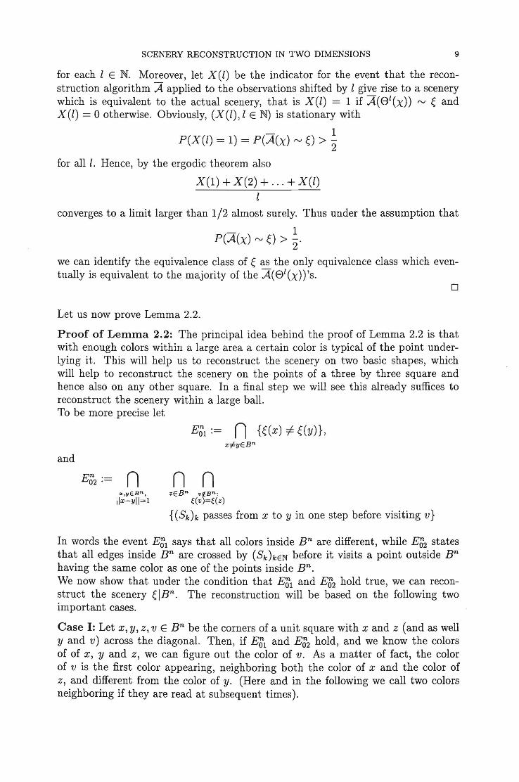
for each lEN. Moreover, let X(l) be the indicator for the event that the recon­struction algorithm A applied to the observations shifted by 1 give rise to a scenery which is equivalent to the actual scenery, that is X(l) = 1 if A(8l (X)) rv ~ and X(l) = 0 otherwise. Obviously, (X(l), lEN) is stationary with

- 1 P(X(l) = 1) = P(A(X) rv 0 > 2

for alll. Hence, by the ergodic theorem also

X(l) + X(2) + ... + X(l) 1

converges to a limit larger than 1/2 almost surely. Thus under the assumption that

- 1 P(A(x) rv 0 > 2·

we can identify the equivalence class of ~ as the only equivalence class which even­tually is equivalent to the majority of the A( 8 l (X)) 's.

o

Let us now prove Lemma 2.2.

Proof of Lemma 2.2: The principal idea behind the proof of Lemma 2.2 is that with enough colors within a large area a certain color is typical of the point under­lying it. This will help us to reconstruct the scenery on two basic shapes, which will help to reconstruct the scenery on the points of a three by three square and hence also on any other square. In a final step we will see this already suffices to reconstruct the scenery within a large ball. To be more precise let

and

E n . 02·= n

:t,yEBn,

iix-yii=l

E~l:- n {~(x) =F ~(y)}, xi:yEBn

n n zEBn v¢Bn:

€(v)=€(z)

{(Sk)k passes from x to y in one step before visiting v}

In words the event EOI says that all colors inside Bn are different, while E02 states that all edges inside Bn are crossed by (SkhEN before it visits a point outside Bn having the same color as one of the points inside Bn. We now show that under the condition that EOI and E02 hold true, we can recon­struct the scenery ~IBn. The reconstruction will be based on the following two important cases.

Case I: Let x, y, z, v E Bn be the corners of a unit square with x and z (and as well y and v) across the diagonal. Then, if EOl and E02 hold, and we know the colors of of x, y and z, we can figure out the color of v. As a matter of fact, the color of v is the first color appearing, neighboring both the color of x and the color of z, and different from the color of y. (Here and in the following we call two colors neighboring if they are read at subsequent times).

10 M. LOWE AND H. MATZINGER

Case II: Let Xl, X2, X3, X4, Y E Bn be a "cross" with center y , that is Xl, X2X3, X4, Y are pairwise different and

IXI - yl = IX2 - yl = IX3 - yl = IX4 - yl = 1.

Knowing that Eoi and E02 hold as well as the colors of Xl, X2, X3 and y we can find out the color of X4 as the only color neighboring ~(y) different from ~(Xl)' ~(X2)' and ~(X3).

We will now see that these two basic techniques suffice to reconstruct ~IBn, if EOI and EO'z hold. Indeed, denoting by Qj the 2j + 1 by 2j + 1 square with center zero, we can first reconstruct ~IQl' To this end we first recover the color of the origin (which is, or course, trivial) and the the colors of (1,0), (0, 1), (-1,0), and (0, -1). Indeed, the colors themselves are known from the observations. Their relative position to each other (which is all we need, because we only want to reconstruct up to equivalence) can be detected from the fact that the color of y can be read with distance two of the color of X without reading the color of the origin in the meantime (and the same for the colors of v and z, for example), while this is not true for the colors of X and z, or the color of y and v, respectively, where we have to pass zero in between. Once we know the ~1{(1, 0), (0, 1), (-1,0), (0, -I)} up to equivalence we can recon­struct the scenery on Ql by applying Case I to the four corner points of Ql' Now we can proceed inductively. Knowing the ~IQj n Bn, we want to reconstruct ~IQj+l n Bn, that is we want to find out the color of the boundary points of Qj+!

(as far as they are inside Bn). For all points with at least one coordinate different from 2j + 1, 2j, -2j - 1, or -2j, this can be done by applying the technique of Case II. Then the color of the points with one coordinate equal to 2j or -2j can be reconstructed by applying the technique of Case I. Finally the same technique yields the color of the corner points of Qj+!.

This shows that under the condition that EOI and E02 hold true we can reconstruct ~IBn up to equivalence. It remains to understand that both, EOI and E02 hold true with arbitrary large probability for fixed n and large enough m. Indeed, this is not very hard to see. For E Ol ' note that

1 P( (EOl)C) :::; const n2_, m

which can be made arbitrarily small by choosing m large. Similar techniques apply to E02 ' Note that by taking T large enough the random walk (Sk)k<T up to time T has visited each point in Bn, at least L times (L some number to be chosen soon, d. [10] for similar results). Then the probability that there is an edge in Bn the random walk does not visit up to time T is bounded by

cons\ n' (~r, which is arbitrarily small for L large enough. If we now first choose L, the take T as above, and finally choose m so large that also the probability that all colors in BT are distinct (by the same techniques as above) is as large as we want to, we see that

p( (E02Y) :::; c

for each c > 0 if only m is large enough. This finishes the proof of Lemma 2.2. 0

SCENERY RECONSTRUCTION IN TWO DIMENSIONS 11

Next we will prove Lemma 2.3, which is indeed the key ingredient to the proof of Theorem 1.1.

Proof of Lemma 2.3: Let En denote the event that given a piece of scenery 't/J with 't/J rv ~IBn the "reconstruction algorithm at step n" A produces a piece of scenery A('t/J, X) with

We need to show that with probability one En holds for all but a finite number of n's (in the following we will also say that an event holds for almost all n if it holds for all n but a finitely many). To do so see we decompose En for n E N in such a way that

En :) E~ n E; n E;. We will then show that each of Ei, i = 1,2,3 holds for all but finitely many n's.

Whenever in the sequel we will say about a piece of scenery 't/J that "'t/J appears in A with starting point x", or "'t/J appears in A with endpoint y", respectively, where 't/J E {O, ... ,m _1}1 for some l, A ~ Z2, and x,y E Z2, we will mean that

xIT='t/J for some realisation of the random walk Sn, some discrete time interval T = [to, to + l - 1] such that Sto = x (or Sto+l-l = y, respectively) and SIT c A. In other words 't/J appears in A with starting point x (or endpoint y) if it can be read in­side of A by a nearest neighbor walk starting in x (ending in y). Moreover if, for one of the line segments o-(v), a-(v), O'(v), cp(v) or ..\(v) , we refer to ~IC (C E {o-(v), a-(v), O'(v), cp(v), ..\(v)}) we mean the observations obtained by reading ~ along C from the center of Bn to the outside of Bn Now let

E~:= nXEBexp(n<l<) {There are less than n(3 different word from

sn appearing in ~1(B;2 \ Bn)},

where B;/ stands for the discrete ball of radius n 2 centered in x. Observe that the definition of Tn implies that on E~ we have that Sk E Bn+n2 for all k E Tn. Moreover let

with

E;l:- n n {~IO'(v) appears in ~IBn2+n only with starting point point inside 1l(v)}, vEflBn u(v)

E;2:= n n{~Ia-(v)appears in ~IBn2+n only with endpoint x E Q2(V)}, vEflBn u(v)

E;3:= n n{~I..\(v)appears in ~IBn2+n only with endpoint x E Q3(V)}, vEflBn >.(v)

E;4:= n n{~lp(v)appears in ~IBn2+n only with endpoint x E Q4(V)}, vE!lBn p(v)

12 M. LOWE AND H. MATZINGER

and

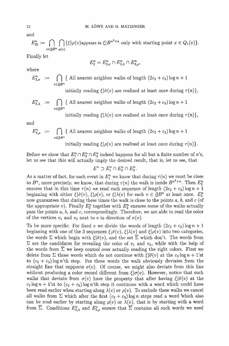
E;5:= n n{~I<p(v)appears in ~IBn2+n only with starting point x E QI(V)}. vEf!.Bn cp(v)

Finally let

where

E;'u·- n {All nearest neighbor walks of length (2C2 + C3) log n + 1

initially reading ~Io-(v) are realized at least once during r(n)},

E;>. .- n , { All nearest neighbor walks of length (2C2 + C3) log n + 1 vEf!.Bn

initially reading ~IA(V) are realized at least once during r(n)},

and

E;'p n { All nearest neighbor walks of length (2C2 + C3) logn + 1 vEf!.Bn

initially reading ~Ip(v) are realized at least once during r(n)}.

Before we show that Ef n E'2 n E'3 indeed happens for all but a finite number of n's, let us see that this will actually imply the desired result, that is, let us see, that

En :J E~ n E; n E; .

As a matter of fact, for each event in Ef we know that during r(n) we must be close to Bn, more precisely, we know, that during r(n) the walk is inside Bn2+n. Then E; ensures that in this time r(n) we read each sequence of length (2C2 + C3) logn + 1 beginning with either ~Io-(v), ~Ip(v), or ~IA(V) for each v E {tBn at least once. E'2 now guarantees that during these times the walk is close to the points a, b, and c (of the appropriate v). Finally E'2 together with E'3 ensures some of the walks actually pass the points a, b, and c, correspondingly. Therefore, we are able to read the color of the vertices VI and V2 next to v in direction of (/( v).

To be more specific: For fixed v we divide the words of length (2C2 + C3) log n + 1 beginning with one of the 3 sequences ~Io-(v), ~IA(V) and ~Ip(v) into two categories, the words L: which begin with ~Io-(v), and the set L: which don't. The words from L: are the candidates for revealing the color of VI and V2, while with the help of the words from L: we keep control over actually reading the right colors. First we delete from L: those words which do not continue with ~IO'( v) at the c2log n + 1 'st to (C2 + C3) logn'th step. For these words the walk obviously deviates from the straight line that supports (/( v). Of course, we might also deviate from this line without producing a color record different from ~I(/(v). However, notice that such walks that deviate from (/( v) have the property that after having ~Io-( v) at the c2logn + l'st to (C2 + c3)logn'th step it continues with a word which could have been read earlier when starting along A( v) or p( v). To exclude these walks we cancel all walks from L: which after the first (C2 + C3) log n steps read a word which also can be read earlier by starting along p( v) or A( v), that is by starting with a word from L:. Conditions E;,>. and E3,p ensure that L: contains all such words we need

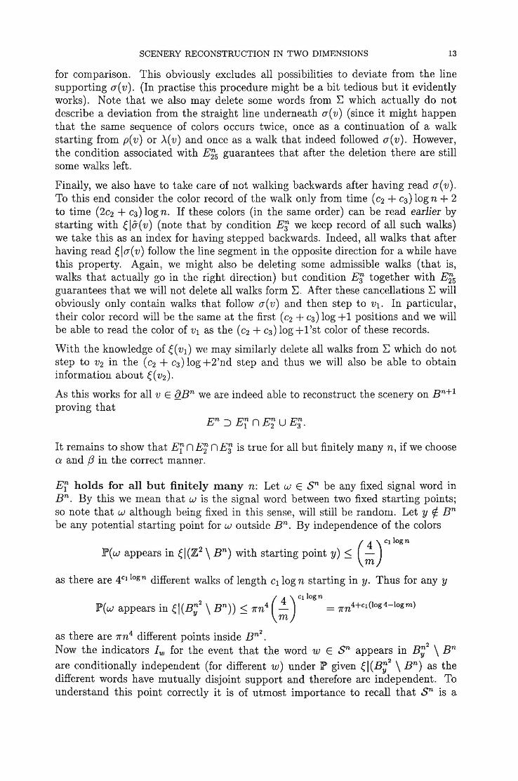
SCENERY RECONSTRUCTION IN TWO DIMENSIONS 13

for comparison. This obviously excludes all possibilities to deviate from the line supporting 0"( v). (In practise this procedure might be a bit tedious but it evidently works). Note that we also may delete some words from L: which actually do not describe a deviation from the straight line underneath 0"( v) (since it might happen that the same sequence of colors occurs twice, once as a continuation of a walk starting from p(v) or >.(v) and once as a walk that indeed followed O"(v). However, the condition associated with E~5 guarantees that after the deletion there are still some walks left.

Finally, we also have to take care of not walking backwards after having read 0"( v). To this end consider the color record of the walk only from time (C2 + C3) logn + 2 to time (2C2 + C3) log n. If these colors (in the same order) can be read earlier by starting with ela-(v) (note that by condition E; we keep record of all such walks) we take this as an index for having stepped backwards. Indeed, all walks that after having read elO"( v) follow the line segment in the opposite direction for a while have this property. Again, we might also be deleting some admissible walks (that is, walks that actually go in the right direction) but condition E'3 together with E~5 guarantees that we will not delete all walks form L:. After these cancellations L: will obviously only contain walks that follow O"(v) and then step to VI. In particular, their color record will be the same at the first (C2 + C3) log + 1 positions and we will be able to read the color of Vl as the (C2 + C3) log + 1 'st color of these records.

With the knowledge of e(VI) we may similarly delete all walks from L: which do not step to V2 in the (C2 + C3) log +2'nd step and thus we will also be able to obtain information about e( V2).

As this works for all v E {lBn we are indeed able to reconstruct the scenery on Bn+! proving that

It remains to show that Er n E~ n E; is true for all but finitely many n, if we choose a and /3 in the correct manner.

Er holds for all but finitely many n: Let w E sn be any fixed signal word in Bn. By this we mean that w is the signal word between two fixed starting points; so note that w although being fixed in this sense, will still be random. Let y ~ Bn be any potential starting point for w outside Bn. By independence of the colors

(4) C} logn P(w appears in el(Z2 \ Bn) with starting point y) ~ m

as there are 4CJ logn different walks of length c1logn starting in y. Thus for any y

( 4) CJ logn lP(w appears in el(B;2 \ Bn)) ~ 7rn4 m = 7rnHCJ (log4-1ogm)

as there are 7rn4 different points inside Bn2. Now the indicators Iw for the event that the word w E sn appears in B;2 \ Bn are conditionally independent (for different w) under lP given el(B;2 \ Bn) as the different words have mutually disjoint support and therefore are independent. To understand this point correctly it is of utmost importance to recall that sn is a

14 M. LOWE AND H. MATZINGER

random set (under lP). The independence claimed above would not be true for any fixed set of words or if we did not condition on knowing ~1(B;2 \ Bn). Hence the number of w E sn appearing in B;2 \ Bn is stochastically bounded by a Binomial random variable with N = n 2 I c1log n different trials and success probability p = 1rn2+Cl(1og4-iogk). By concentration of measure, (or the simple fact the the rate function of a large or moderate deviation principle for i.i.d. Bernoullis can be quadratically bounded), cf. [12], for N i.i.d. Bernoullis Xi with success probability p we have that

i=l

for each N and each ~ > O. Applying this to our situation and moreover choosing m in such a way that

1rn2+Cl (iog4-iogm) :::; lin

(which is possible for every fixed Cl) yields

lP(There are more than n(3 different words from sn in ~IB;2 \ Bn)

for each positive c > 0 and n large enough. Hence _n2(!3-1)-< 2n'" _n2(!3-1)-<

e = 1re e xEBexp(n"')

(3.1)

As a < /3, and we can choose them such that 2/3 - 2 > a + E the right hand side of (3.1) clearly is summable in n, which by the Borel-Cantelli Lemma yields that E''i holds for all but finitely many n.

E2 holds for all but a finite number of n: Since the proofs of that E2i holds for almost all n are very similar for each i, we just show it for E22 and leave the other proofs to the reader. To this end consider any v E !lBn and any oriented connected segment s in 'Z} of length c2log n. Note that if the endpoint of s is not in Q2 the i'th point of 0-( v) is different from all the j'th points of s, j :::; i, and thus ~(o-i(V)) is a "fresh random variable. Thus by conditional independence the probability of reading 0-( v) along ~Is is bounded by

( 1 ) C2

iog

n

lP(~ls = o-(v)):::; m '

and therefore for every fixed x E Bn2+n \ Q2 (v)

(4) C2io

gn

lP(o-(v) appears with endpoint x):::; m

As there are at most 1r(n2 + n)2 points in Bn2+n and there are at most canst x n points v E !lBn, we obtain

(4) C2io

gn

lP((E;2Y):::; m canst x n1r(n2 + n? = nC2 (iog4-iogm)

SCENERY RECONSTRUCTION IN TWO DIMENSIONS 15

The right hand side of this inequality becomes summable if we choose m large enough (depending on C2 - or C3 when we want to prove that another E2i holds). This choice of m will basically be the proof of Theorem 1.1. Thus (again by a Borel-Cantelli argument) E22 holds true for all but finitely many n.

Note that until now we are still free to choose C1, C2, C3'

E3 holds for all but finitely many n: Again we only give the proof in detail for one of the events, which will be E3 u' The proof for the other two events follows the same lines. '

We split this proof into several parts. First let us prove that in a certain (stricter than usual) sense the random walk by time en'" has returned to the origin more than n'Y times, where 'Y < a < f3. A result like this seems to be very much in the spirit of a result by Erdos and Taylor [2], who showed that almost surely a random walk at time en has returned to the origin between n/(logn)1+e and (1 + c)n log logn times for all but finitely many n's and every positive c > O. The reason why we cannot simply refer to this result is that we also want these returns to the origin to be apart at least n2 from each other. So, more precisely let us introduce a sequence {}i of stopping times such that {}(j = 0 for all nand {}i+1 is the time of the first return of the random walk Sk to the origin after time {}i + n2• This will ensure that in the meantime the random walk is able to hit one of the boundary points of Bn. So we want to check that for 'Y < a < f3 ('Y appropriately chosen afterwards) the event

E~l := {{}~"f ::; en"'}

happens for all but finitely many n's. Indeed, choosing () = U? the result by Erdos and Taylor [2] quoted above states that the event

E~l1 := { Up to time en'" there are more than n'YH returns to the origin}

holds true almost surely for all but a finite number of n's. Next we will show that the same is true for the event

n"f

E~12 := n{In the interval [{}f, {}f+n2] there are less than nO returns to the origin }. i=l

As a matter of fact the probability for a simple random walk to start in the origin and not to return to it for t steps is bounded below by l~;t for t large enough [11, p.167], [3]. Applying this yields

JP(In the interval [{}f, {}f + n2] there are more than nO returns to the origin)

< (1 7r) n

6

::; e-n6/2

- logn

for each i = 1, ... ,n'Y and n large enough. Hence by bounding the probability of a union by the sum of the probabilities

JP((E~12)C) ::; n'Ye-n6/2

which is finitely summable. Therefore E312 holds for all but a finite number of n's. As E311 and E312 together imply E31 also E31 holds for almost all n.

16 M. LOWE AND H. MATZINGER

Next we will show that many of the intervals ['!?i, '!?i + n2] above are indeed signal times, that is we will show that we read more than nf3 different signals in all of these time intervals. To this end introduce random variables Yi which are indicators for the event that the interval ['!?i, '!?i + n2 ] is a signal time, that is for the event that there are more than n f3 signal words read in ['!?i, '!?i + n2

]. To avoid the dependence among reading different signal words we only concentrate on such words which are "far apart" form each other. To this end we partition the inner part of En, that is En \ o(logn)3En where

O(logn)3En := {x E Bn, d(x,QEn) ~ (logn)3}

and d(·, .) is the lattice distance in Z2, into boxes of lengths c1log n and (log n)3. Let

Wk,l := {(x, y) E B n : k logn ~ x ~ (k 1) logn, l (logn)3 ~ y < (l + 1)(logn?},

(k, l E Z).

Now consider the following indicators: Let I1,n( i) be the indicator for the event that SUi+

n¥ E En/logn. H2,n(i) denotes the indicator for the event that the whole

trajectory (Sk)k=U?, ... ,u?+n¥ is contained in En. Furthermore, let J[3,n(i) be one if

the random walk visits more than n2(lt

P) /(2(1:/3) logn) distinct points in ['!?i,'!?i +

!±l!] d h' n 3 an zero ot erWlse. Moreover let lIk'7( i) be the indicator for the event that in the time interval ['!?i, '!?i + n!¥ 1 the walk' enters Wkl and within (log n)3 steps after the first entrance time touches one of the lines ~ = k log n or x = (k + 1) log n, and finally follows the straight line supporting the the word associated with the starting point it touched.

First consider the event {J[l,n( i) = O}. By concentration of measure (cf. [12]) we have for every fixed i

¥ p(H1,n(i) = 0) = P(IIS 4+1311 ~ n ~ e -const'(~ogn)2

t??+n-r logn Therefore, as f3 < 2

which is finitely summable and thus ni{][2,n(i) 1} holds true for almost all n.

By the same argument " !±l!

p(I2,n(i) = 0) - P(3t E ['!??,'!?? + n 3 ] : IIStil ~ n) ,.2-fJ

< n2P(IISu~+n1¥ II ~ n) ~ n2e-const·-3-. ,

Thus, also ni{][2,n(i) = O} holds true for "all but finitely many n.

To bound the probability that ][3,n( i) is equal to zero, first observe that the number of distinct points D t visited by a simple symmetric random walk starting in the origin by time t satisfies (cf.[4J, [3])

2t EDt >­

- logt

SCENERY RECONSTRUCTION IN TWO DIMENSIONS 17

for all t large enough. Moreover such a random walk clearly can only have visited at most t points (Le. Dt :::; t) up to time t. Together this implies

t 1 P(Dt> -)<-.

- logt - logt (3.2)

Partitioning the interval [{)i, {) i + n ~] into n ¥ intervals of length n 2!¥ and ap­plying (3.2) with t = nZ!¥ (observe that logt = 21~,8logn) yields for any fixed i:

canst. < -Con8t.~ )n¥ ¥

-- e logn.

logn -

Hence by the same summability argument as above ni {JI3,n( i) = I} holds for almost all n.

Next let us have a closer look at {JIk'7(i) = I}. Suppose that we already know that

Sn enters the sector Wkl within [{)i,'{)i + n~]. Considering just the projection of the walk to the x-axes, 'we see a nearest neighbor random walk on Z with holding probability 1/2. The points k log nand (k + 1) log n obtained by projecting the vertical limiting lines of Wkl may be considered absorbing barriers for this random walk. As the expected hitti~g time of one of these barriers is of order (log n)2, after time (log n? we will have hit one of the boundaries with a probability bounded away from zero (in n). In other words that is to say, that Sn conditioned on that it will visit Wkl at all, will touch one of its left and right boundary lines within (logn)3 after the first' entrance time into this sector with probability bounded away from zero. As the word associated to this boundary point has length Cl log n the probability that the walk touches a boundary point and then follows the walk associated to it is bounded by canst. (1/4 )c1log n.

Note that the events {JIk'r( i) = I} are not independent for different choices of (k, 1) and the same i and n. First due to the fact that (Sk) is a Markov chain the event {n!'r( i) I} increases the chances that we also hit a square close to Wk /' However, als~ given that we visit both Wk,l and Wlk+1),1 for example, the events {n!:r( i) = I} and {JI!:;\/ i) = I} are dependent since reading a word associated with a boundary poin: of Wk,n might easily coincide with touching a boundary point of Wk+1,n less than (logn)3 steps after the first entrance time. To cope with this effect we disregard every other square, that is we consider the indicators

n!'r(i) := ][:'~(i)n(k, l) , ,

where JI(k, l) is +1 if k and l are even and 0 otherwise, instead.

Now observe that on {JI2•n(i) = I} n {JI3,n(i) = I} the random walk visits more than n2!¥ /2{li,8) log n distinct points within [{)i, {)i + n~J - all of them lying in Bn

and therefore, as each of the Wk,l has cl(logn)4 points, also nZ!¥ /(2Cll~.B(logn)5) distinct Wk,I'S. As one fourth of them will have both k and I even n!:r( i) has a

chance to become +1 for n2!¥ /(8Cll~.B(logn)5) different choices of (k, l). Given the indices (k,l) for which this is true the events {i:'~( i) = I} indeed are independent ,

18 M. LOWE AND H. MATZINGER

and have probability at least canst.(1/4)Cllogn. Hence again by moderate deviations or concentration of measure on {1I2,n( i) = I} n {1I3,n( i) = I}

"""' A4 n.B n3 e

(

1(2-.B)-q log 4) IP(L..,.lIk:l (i) ::; n ) ::; exp -canst. (logn)lO ::; e-n

k,l

for some small c, if Cl is small enough (depending on how large we have chosen f3 before). As e-ne is finitely summable even after multiplication with the number of different {)i we obtain that on the event ni{{1I2,n(i) = I} n {1I 3,n(i) = I}} we have 2:klft!'7(i) ~ n.B for all i and all but finitely many n's. As also ni{{1I2,n(i) = I} n {1I3,~( i) , = I} } holds for almost all n

L ft!;7(i) ~ n.B k,l

also is true for almost all n. As finally also ni{1I1,n(i) = I} for all but a finite number of n's, we arrive at n{ {Yi = I} n {1I1,n( i) = I} }

i

for all n but finitely many.

Let us summarise what we know already. For almost all n the following holds true: Until time enD< we have more than n'Y (t smaller than 00') different intervals of length

n2 of signal times. The signals are read in the first n!¥ steps, after which the random walks stops in a distance at most n/log n from the origin.

Finally we have to show that in these time intervals [{)i, {)i + n 2] we also read all words of length (2C2 + C3) log n beginning with either a root word or a side word associated to any of the boundary points. To avoid trouble with independence we will only concentrate on events where this happens in one of the time intervals I n .- [_an !±1! .an 2]· - 1 2 i .- Vi +n 3 'Vi +n ,~- , , .... To this end, first observe that (Sk) on Ji has variance

V !±1! n n2 - n 3 >­- 2

for n large enough. Therefore, and since "in the worst case" Sn~ = 0 with positive

probability bounded away from zero (Sk) exits Bn during Ji . This bound will be used to estimate the probability to hit the beginning ClO(V) of a root word for a boundary point v E flBn or the beginning of one of its side words. This probability can be computed as the probability of hitting this point conditioned on that we hit the (discrete) sphere it is contained in, times the probability that we hit this sphere at all. The latter probability is bounded below by a constant away from zero, by the above considerations. On the other hand the probability to hit a certain point in flBn conditioned on that we leave Bn is bounded below by ~ for some constant x > 0 no matter where in Bn/logn we started. Of course, it suffices to understand that this is true for large n. But observing that under the scaling Z2 -t ~Z2, the boundary flBn converges to the unit sphere, Bn/logn shrinks to the origin and (Sk) converges (after rescaling also the time axes which is irrelevant for our argument) to Brownian motion WO(t) starting in the origin and moreover taking into account that the harmonic measure on the unit sphere (any sphere centered in zero) with respect

SCENERY RECONSTRUCTION IN TWO DIMENSIONS 19

to WO(t) is the uniform distribution on it, shows that the above bound indeed holds. So, as all starting points of root words and side words lie in Bn2 \ Bn

2-(c2+c3)logn we see that the probability of hitting any fixed starting point is bounded from below by :, for some x' > 0 (x' results from multiplying x with the probability of exiting Bn2 in a certain Ji ).

Now the probability of reading 0-( v) and after that any fixed continuation of length (C2 + C3) logn given that we first read O'o(v) has (for any fixed v E {lBn) probability

_ = n-(2c2+c3)log4. (1) (2C2+C3) log n

4

So the (unconditioned) probability of reading o-(v) and after that any fixed contin­uation of length (C2 + C3) log n is bounded below by

(1) (2C2+C3) logn : 4 = xn-1-(2c2+C3)log4.

On the other hand there are n'Y different time intervals where we can read such a word. So the probability of not reading 0-( v) and after that any fixed continuation of length (C2 + C3) log n in all of these intervals behaves like

( 1 _ ""-1-(2,,+,,,) log 4 ) n' <:; exp ( _ ",,7-1-(2"+,,,) log4).

As we can choose C2 and C3 as small as we want to and I > 1 (and still I, a) this probability is smaller than e-ne for some E > O. The same holds true for the probability of reading a side word and then any fixed continuation of length (C2 + C3) log n given that we read its first letter. As for fixed n there are only polynomially many of such words (more precisely, as there less than

67rn4(c2+c3)logn = 67rn1+(C2+c3)log4

such words) the probability of not reading all of them is bounded by

67rn1+(C2+C3) log4e-n <

which is finitely summable in n. Therefore, by the Borel-Cantelli Lemma, also E~ holds for all but finitely many n's. This finishes the proof of Lemma 2.3. 0

The proof of the main theorem now only consists of choosing the constants in the correct order.

Proof of Theorem 1.1: To finish the proof we finally specify the order in which we choose the constants. So first we choose a, /3, I with 2/3 - 2 > a (such that right hand side in (3.1) is finitely summable), and 1 < I < a. Then we choose CI, C2 and C3 to make the last part of the above proof of Lemma 2.3 work (note that this part does not depend on the number of colors m). If we now choose m larger than a certain number ml (coming from the arguments which guarantee that El and E;: hold), this procedure ensures that the reconstruction in Lemma 2.3 works with probability one for almost all n. Call the largest n for which it does not work N. Then according to Lemma 2.2 for each E > 0 there is a number m2 and a reconstruction algorithm AN such that if m ~ m2 we can reconstruct ~IBN with probability larger than 1 - E. If we now choose m ~ max{ml, m2} and concatenate AN from Lemma 2.2 with An

20 M. LOWE AND H. MATZINGER

for n ~ N + 1 from Lemma 2.3, we obtain an algorithm A which reconstructs ~ with probability larger than 1 - c.

In view cf Lemma 2.1 this suffices to prove Theorem 1.1. o

REFERENCES

[1] I. Benjamini, H. Kesten; Distinguishing sceneries by observing the sceneries along a random walk path, J. d'Ana!. Math 69, 97-135 (1996)

[2] P. Erdos, S.J. Taylor; Some problems concerning the structure of random walk paths, Acta Math. Acad. Sci. Hung. 11, 137-162 (1960)

[3) D. Downham, S. Fotopolous; The transient behaviour of the simple random walk in the plane, J. Appl. Prob. 25, 58-69 (1988)

[4] A. Dvoretzky, P. Erdos; Some problems on random walks in space, Proc. 2nd Berkeley Math. Stat. Prob., 353-367 (1951)

[5) W. Th. F. den Hollander, M. Keane; Ergodic properties of color records, Physica 138A, 183-193 (1986)

[6] H. Kesten; Distinguishing and reconstructing sceneries from observations from random walk paths, Microsurveys in discrete probability (D. Aldous and J . Propp, eds.), DIMACS Series in Discrete Mathematics and Theoretical Computer Sciences 41, 75-83 (1998)

[7] E. Lindenstrauss; Indistinguishable Sceneries, random Struct. Alg. 14, 71-86 (1999) [8) H. Matzinger; Reconstructing a 3-color scen~ry by observing it along a simple random

walk, Preprint, to apper in: Random Struct. Alg. (1997) [9] H. Matzinger; Reconstruction of a one dimensional scenery seen along the path of a

random walk with holding, Ph. D. Thesis, Cornell University (1999) [10] P. Revesz; Estimates on the largest disc covered by a random walk, Ann. Prob 18,

1784-1789 (1990) [11] F. Spitzer; Principles of random walk, Van Nostrand, London (1964) [12] M. Talagrand; A new look at independence Ann. Prob 24, 1-34 (1996)

(Matthias Lowe) EURANDOM, PO Box 513, NL-5600 MB EINDHOVEN, THE NETHERLANDS E-mail address.MatthiasLowe:lowe@eurandom.tue.nl

(Heinrich Matzinger) EURANDOM, PO Box 513, NL-5600 MB EINDHOVEN, THE NETHERLANDS E-mail address.HeinrichMatzinger:matzinger@eurandom.tue.nl