Scenario-based Capital Requirements for the InterestRate Risk of Insurance Companies

Sebastian Schlutter∗

28th April 2017

Abstract

The Solvency II standard formula measures interest rate risk based on two stressscenarios which are supposed to reflect the 1-in-200 year event over a 12-month timehorizon. The calibration of these scenarios appears much too optimistic when com-paring them against historical yield curve movements. This article demonstratesthat interest rate risk is measured more accurately when using a (vector) autore-gressive process together with a GARCH process for the residuals. In line withthe concept of a pragmatic standard formula, the calculation of the Value-at-Riskcan be boiled down to 4 scenarios, which are elicited with a Principal ComponentAnalysis (PCA), at the cost of a relatively small measurement error.Keywords: Interest Rate Risk, Principal Component Analysis, Capital Require-ments, Solvency IIJEL classification: G17, G22, G32, G38

∗University of Applied Sciences Mainz, School of Business, Lucy-Hillebrand-Str. 2, 55128 Mainz,Germany; Fellow of the International Center for Insurance Regulation, Goethe University Frankfurt;Email: sebastian.schluetter@hs-mainz.de

1

1 Introduction

Interest rate risk is one of the most significant risks of insurance companies. Since insurers

are facing long-term obligation, they invest over long time horizons, and a large portion of

their assets are fixed income investments such as bonds or mortgage loans. Typically, the

durations of assets and liabilities are not matched, but life insurers attain much longer

durations on their liability side than on their asset side.1 Modern insurance regulation

frameworks, such as Solvency II in the European Economic Area, impose risk-based

capital requirements to address those risks. Under Solvency II, the capital requirement

is defined as the 99.5% Value-at-Risk of the change in economic capital over one year.2

Most insurers determine the capital requirement with a standard formula. Regarding

interest rate risks, the standard formula applies multiplicative stress factors to the current

yield curve to determine an upward and a downward shift of interest rates, and insurers

need to recalculate their capital in these scenarios. The calibration of the stress factors,

at least for the downward scenario, appears much too optimistic. Between 1999 and

2015, the downward stress scenario underestimated the drop in interest rates during the

subsequent 12 months for periods in 2011 as well as between 2014 and 2015 (EIOPA, 2016,

p. 59). This poor backtesting result is broadly in line with the result of Gatzert and

Martin (2012), who show that the standard formula’s risk assessment of bond investments

is inappropriate when comparing it against a partial internal model. Apart from the

calibration, the standard formula may systematically underestimate the risk of curvature

changes of the yield curve. Since both stress scenarios reflect yield curve shifts, insurers

1EIOPA (2014, p. 17) report that durations of liabilities are on average 10 years longer than those ofassets for Austrian, German, Lithuanian and Swedish insurers.

2Cf. European Commission (2009), Art. 101 (3).

2

can immunize against them by closing the duration gap.3 The capital requirement may

thereby drop (close) to zero. However, insurers are still vulnerable to changes in the

curvature.

The objective of this article is to derive a model for interest rate risk which is applicable

for a regulatory standard formula. The model should fulfill the following properties:

1. The model should allow for determining the Solvency II capital requirement (i.e.

99.5% Value-at-Risk with a 1-year holding period).

2. The capital requirement should pass backtesting against historical yield curve move-

ments.

3. The capital requirement should reflect the insurer’s exposure to curvature changes

of interest rates.

4. It should take into account that there is a lower bound to interest rates reflecting

the economic costs of storing cash.

5. It should be a pragmatic approach, which insurers can implement for example by

recalculating their economic equity capital in a small number of scenarios.

In the first part of this paper, we develop a model that is intended to fulfill properties 1-4.

To this end, two models stand as candidates. The first candidate model focuses on the

4 parameters of the Nelson and Siegel (1987) model or 6 parameters of the extension by

Svensson (1994) which both represent the whole yield curve. Diebold and Li (2006) derive

good forecasts of future yield curves by modeling the development of these parameters

3Cf., e.g., Litterman and Scheinkman (1991, p. 55 f.) who explain how to construct a portfolio thatis immunized against a particular movement (not necessarily parallel) of the yield curve.

3

over time with stochastic processes. In particular, the forecasts outperform those of

affine factor models, which we therefore do not use in this paper.4 Caldeira et al. (2015)

build on the procedure of Diebold and Li (2006) to estimate the Value-at-Risk of fixed

income portfolios with a 1-day holding period. For longer holding periods, in particular

when being situated in a low yield environment, it becomes relevant whether the model

could simulate arbitrarily high negative interest rates or accounts for a lower bound (cf.

property 4 above). Unfortunately, we are not aware of an easy extension of the approach

from Caldeira et al. (2015) to incorporate a lower bound.5

As a second candidate model, we suggest a two-step approach which is particularly de-

signed to respect such a lower bound. In a first step, the interest rates for 5 key maturities

are modeled, each as the logarithmic distance to a lower bound. The development of the

5 key maturity interest rates over time is described by a (vector) autoregressive process

together with a multivariate GARCH process for the residuals. In a second step, we use

the Svensson model to interpolate and extrapolate the 5 interest rates to the complete

term structure.

We backtest the Value-at-Risk estimates of both candidate models for relatively high

confidence levels and relatively long holding periods against historical data. To address

properties 2 and 3, the backtesting is conducted for 1,000 portfolios whose payoffs and

maturities are randomly chosen.6 For a given portfolio, the accuracy of the Value-at-Risk

is measured by the portion of historical time windows in which the Value-at-Risk under-

4The weak performance of affine factor models to forecast the yield curve has also been demonstratedby Duffee (2002). Moreover, by modeling the short rate, affine factor models focus on yield curve shiftsand may therefore underestimate the risk of curvature changes when being used for capital requirements.

5Eder et al. 2014 propose incorporating a lower bound for interest rates by means of a plane-truncatednormal distribution. However, the approach is numerically extensive and it therefore seems difficult tocombine it with a GARCH process to address heteroscedasticity in longer time horizons.

6The backtesting in this case is more challenging than the one performed by Caldeira et al. (2015),who focus on the Value-at-Risk of equally-weighted portfolios.

4

estimates the loss in value that the portfolio had experienced for the actual change in

interest rates (hit rate). Across all portfolios, the accuracy of the proposed 2-step model

is similar to the dynamic Svensson model. In the context of capital requirements and

resulting incentives for risk management, the model’s accuracy should not substantially

vary across portfolios (otherwise, regulation provides opportunities for regulatory arbi-

trage, since firms are incentivized to realize portfolios with risks that are measured too

optimistically). In this regard, the proposed two-step model performs better than the

dynamic Svensson model, since the standard deviation of the hit rate across portfolios is

smaller. Moreover, from a regulatory perspective, it is important that the Value-at-Risk

exceedances are not concentrated on particular time periods. Again, the proposed model

performs slightly better than the Svensson model.

In the second part of the paper, we derive a scenario-based approximation of the Value-at-

Risk in order to address property 5. The scenarios are elicited by a principal component

analysis from the simulated yield curves according to the model in part 1. When the

proposed two-step model is used for this purpose, the scenarios respect lower bounds

for interest rates as well. The Value-at-Risk is determined by calculating the loss in

capital for each scenario and then aggregating these losses by a square-root formula. A

backtesting with 100,000 randomly chosen portfolios demonstrates that the 99.5% Value-

at-Risk with a 1-year holding period can be closely approximated based on 4 yield curve

stress scenarios.

The remainder of the paper is organized as follows. Section 2 outlines the approaches

for stochastically modeling interest rate risks (part 1) and transforming the Value-at-

Risk into a scenario-based calculation (part 2). Section 3 calibrates the models based on

yield curve data published by the European Central Bank (ECB). Section 4 provides the

5

backtesting of the stochastic models (part 1) as well as of the scenario-based calculation

(part 2). Section 5 concludes.

2 Value-at-Risk for interest rate risk

2.1 Firm model

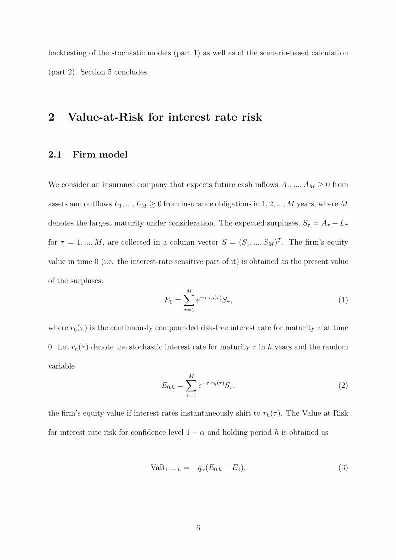
We consider an insurance company that expects future cash inflows A1, ..., AM ≥ 0 from

assets and outflows L1, ..., LM ≥ 0 from insurance obligations in 1, 2, ...,M years, where M

denotes the largest maturity under consideration. The expected surpluses, Sτ = Aτ −Lτ

for τ = 1, ...,M , are collected in a column vector S = (S1, ..., SM)T . The firm’s equity

value in time 0 (i.e. the interest-rate-sensitive part of it) is obtained as the present value

of the surpluses:

E0 =M∑τ=1

e−τ ·r0(τ)Sτ , (1)

where r0(τ) is the continuously compounded risk-free interest rate for maturity τ at time

0. Let rh(τ) denote the stochastic interest rate for maturity τ in h years and the random

variable

E0,h =M∑τ=1

e−τ ·rh(τ)Sτ , (2)

the firm’s equity value if interest rates instantaneously shift to rh(τ). The Value-at-Risk

for interest rate risk for confidence level 1− α and holding period h is obtained as

VaR1−α,h = −qα(E0,h − E0), (3)

6

where qα(X) denotes the α-quantile of the random variable X. The focus of this paper is

the Solvency II requirement for interest rate risk, which is determined as VaRIR99.5%(1 year).

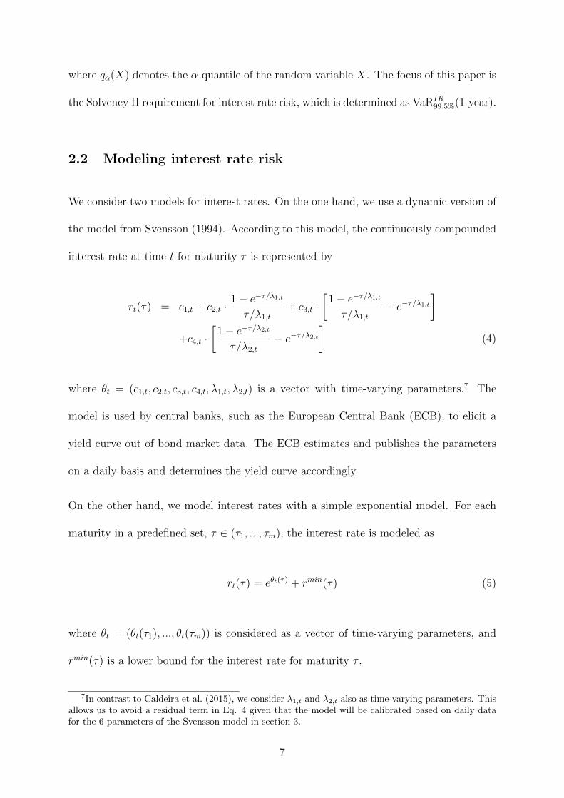
2.2 Modeling interest rate risk

We consider two models for interest rates. On the one hand, we use a dynamic version of

the model from Svensson (1994). According to this model, the continuously compounded

interest rate at time t for maturity τ is represented by

rt(τ) = c1,t + c2,t ·1− e−τ/λ1,tτ/λ1,t

+ c3,t ·[

1− e−τ/λ1,tτ/λ1,t

− e−τ/λ1,t]

+c4,t ·[

1− e−τ/λ2,tτ/λ2,t

− e−τ/λ2,t]

(4)

where θt = (c1,t, c2,t, c3,t, c4,t, λ1,t, λ2,t) is a vector with time-varying parameters.7 The

model is used by central banks, such as the European Central Bank (ECB), to elicit a

yield curve out of bond market data. The ECB estimates and publishes the parameters

on a daily basis and determines the yield curve accordingly.

On the other hand, we model interest rates with a simple exponential model. For each

maturity in a predefined set, τ ∈ (τ1, ..., τm), the interest rate is modeled as

rt(τ) = eθt(τ) + rmin(τ) (5)

where θt = (θt(τ1), ..., θt(τm)) is considered as a vector of time-varying parameters, and

rmin(τ) is a lower bound for the interest rate for maturity τ .

7In contrast to Caldeira et al. (2015), we consider λ1,t and λ2,t also as time-varying parameters. Thisallows us to avoid a residual term in Eq. 4 given that the model will be calibrated based on daily datafor the 6 parameters of the Svensson model in section 3.

7

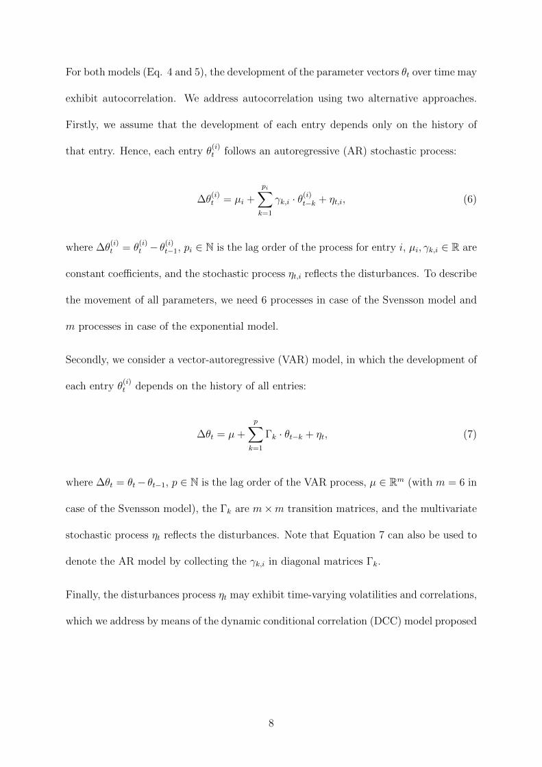
For both models (Eq. 4 and 5), the development of the parameter vectors θt over time may

exhibit autocorrelation. We address autocorrelation using two alternative approaches.

Firstly, we assume that the development of each entry depends only on the history of

that entry. Hence, each entry θ(i)t follows an autoregressive (AR) stochastic process:

∆θ(i)t = µi +

pi∑k=1

γk,i · θ(i)t−k + ηt,i, (6)

where ∆θ(i)t = θ

(i)t − θ

(i)t−1, pi ∈ N is the lag order of the process for entry i, µi, γk,i ∈ R are

constant coefficients, and the stochastic process ηt,i reflects the disturbances. To describe

the movement of all parameters, we need 6 processes in case of the Svensson model and

m processes in case of the exponential model.

Secondly, we consider a vector-autoregressive (VAR) model, in which the development of

each entry θ(i)t depends on the history of all entries:

∆θt = µ+

p∑k=1

Γk · θt−k + ηt, (7)

where ∆θt = θt− θt−1, p ∈ N is the lag order of the VAR process, µ ∈ Rm (with m = 6 in

case of the Svensson model), the Γk are m×m transition matrices, and the multivariate

stochastic process ηt reflects the disturbances. Note that Equation 7 can also be used to

denote the AR model by collecting the γk,i in diagonal matrices Γk.

Finally, the disturbances process ηt may exhibit time-varying volatilities and correlations,

which we address by means of the dynamic conditional correlation (DCC) model proposed

8

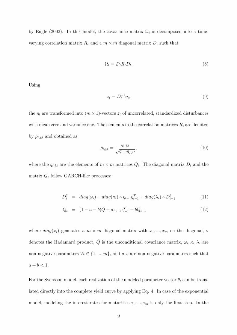
by Engle (2002). In this model, the covariance matrix Ωt is decomposed into a time-

varying correlation matrix Rt and a m×m diagonal matrix Dt such that

Ωt = DtRtDt. (8)

Using

zt = D−1t ηt, (9)

the ηt are transformed into (m× 1)-vectors zt of uncorrelated, standardized disturbances

with mean zero and variance one. The elements in the correlation matrices Rt are denoted

by ρi,j,t and obtained as

ρi,j,t =qi,j,t√qi,i,tqj,j,t

, (10)

where the qi,j,t are the elements of m×m matrices Qt. The diagonal matrix Dt and the

matrix Qt follow GARCH-like processes:

D2t = diag(ωi) + diag(κi) ηt−1ηTt−1 + diag(λi) D2

t−1 (11)

Qt = (1− a− b)Q+ azt−1zTt−1 + bQt−1 (12)

where diag(xi) generates a m × m diagonal matrix with x1, ..., xm on the diagonal,

denotes the Hadamard product, Q is the unconditional covariance matrix, ωi, κi, λi are

non-negative parameters ∀i ∈ 1, ...,m, and a, b are non-negative parameters such that

a+ b < 1.

For the Svensson model, each realization of the modeled parameter vector θt can be trans-

lated directly into the complete yield curve by applying Eq. 4. In case of the exponential

model, modeling the interest rates for maturities τ1, ..., τm is only the first step. In the

9

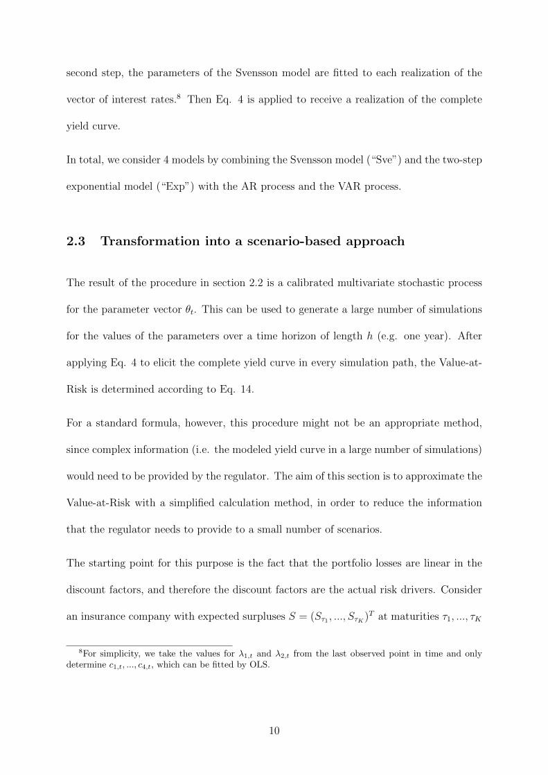
second step, the parameters of the Svensson model are fitted to each realization of the

vector of interest rates.8 Then Eq. 4 is applied to receive a realization of the complete

yield curve.

In total, we consider 4 models by combining the Svensson model (“Sve”) and the two-step

exponential model (“Exp”) with the AR process and the VAR process.

2.3 Transformation into a scenario-based approach

The result of the procedure in section 2.2 is a calibrated multivariate stochastic process

for the parameter vector θt. This can be used to generate a large number of simulations

for the values of the parameters over a time horizon of length h (e.g. one year). After

applying Eq. 4 to elicit the complete yield curve in every simulation path, the Value-at-

Risk is determined according to Eq. 14.

For a standard formula, however, this procedure might not be an appropriate method,

since complex information (i.e. the modeled yield curve in a large number of simulations)

would need to be provided by the regulator. The aim of this section is to approximate the

Value-at-Risk with a simplified calculation method, in order to reduce the information

that the regulator needs to provide to a small number of scenarios.

The starting point for this purpose is the fact that the portfolio losses are linear in the

discount factors, and therefore the discount factors are the actual risk drivers. Consider

an insurance company with expected surpluses S = (Sτ1 , ..., SτK )T at maturities τ1, ..., τK

8For simplicity, we take the values for λ1,t and λ2,t from the last observed point in time and onlydetermine c1,t, ..., c4,t, which can be fitted by OLS.

10

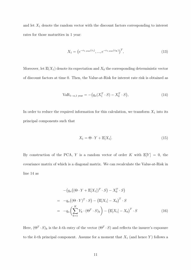
and let X1 denote the random vector with the discount factors corresponding to interest

rates for those maturities in 1 year:

X1 =(e−r1 year(τ1), ..., e−r1 year(τK)

)T, (13)

Moreover, let E(X1) denote its expectation and X0 the corresponding deterministic vector

of discount factors at time 0. Then, the Value-at-Risk for interest rate risk is obtained as

VaR1−α,1 year = −(qα(XT

1 · S)−XT0 · S

), (14)

In order to reduce the required information for this calculation, we transform X1 into its

principal components such that

X1 = Θ · Y + E[X1]. (15)

By construction of the PCA, Y is a random vector of order K with E[Y ] = 0, the

covariance matrix of which is a diagonal matrix. We can recalculate the Value-at-Risk in

line 14 as

−(qα((Θ · Y + E[X1])

T · S)−XT

0 · S)

= −qα((Θ · Y )T · S

)−(E[X1]−X0

)T · S= −qα

( K∑k=1

Yk · (ΘT · S)k

)−(E[X1]−X0

)T · S (16)

Here, (ΘT ·S)k is the k-th entry of the vector (ΘT ·S) and reflects the insurer’s exposure

to the k-th principal component. Assume for a moment that X1 (and hence Y ) follows a

11

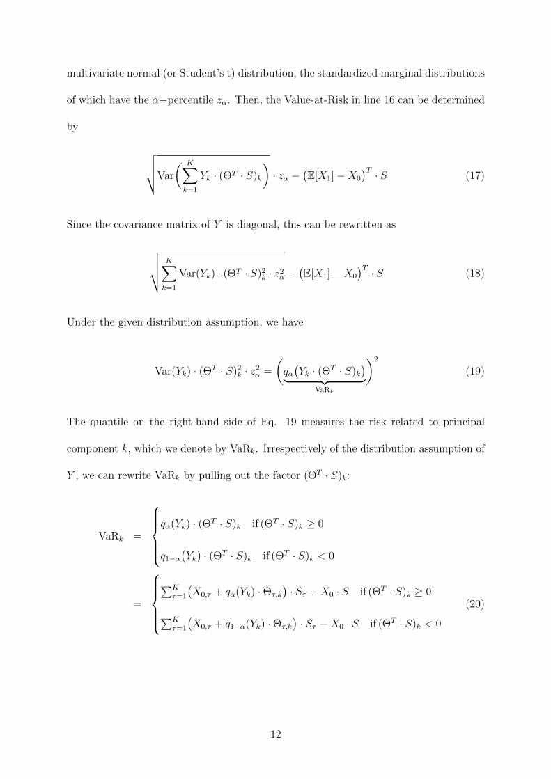
multivariate normal (or Student’s t) distribution, the standardized marginal distributions

of which have the α−percentile zα. Then, the Value-at-Risk in line 16 can be determined

by

√√√√Var

( K∑k=1

Yk · (ΘT · S)k

)· zα −

(E[X1]−X0

)T · S (17)

Since the covariance matrix of Y is diagonal, this can be rewritten as

√√√√ K∑k=1

Var(Yk) · (ΘT · S)2k · z2α −(E[X1]−X0

)T · S (18)

Under the given distribution assumption, we have

Var(Yk) · (ΘT · S)2k · z2α =

(qα(Yk · (ΘT · S)k

)︸ ︷︷ ︸VaRk

)2

(19)

The quantile on the right-hand side of Eq. 19 measures the risk related to principal

component k, which we denote by VaRk. Irrespectively of the distribution assumption of

Y , we can rewrite VaRk by pulling out the factor (ΘT · S)k:

VaRk =

qα(Yk) · (ΘT · S)k if (ΘT · S)k ≥ 0

q1−α(Yk) · (ΘT · S)k if (ΘT · S)k < 0

=

∑K

τ=1

(X0,τ + qα(Yk) ·Θτ,k

)· Sτ −X0 · S if (ΘT · S)k ≥ 0

∑Kτ=1

(X0,τ + q1−α(Yk) ·Θτ,k

)· Sτ −X0 · S if (ΘT · S)k < 0

(20)

12

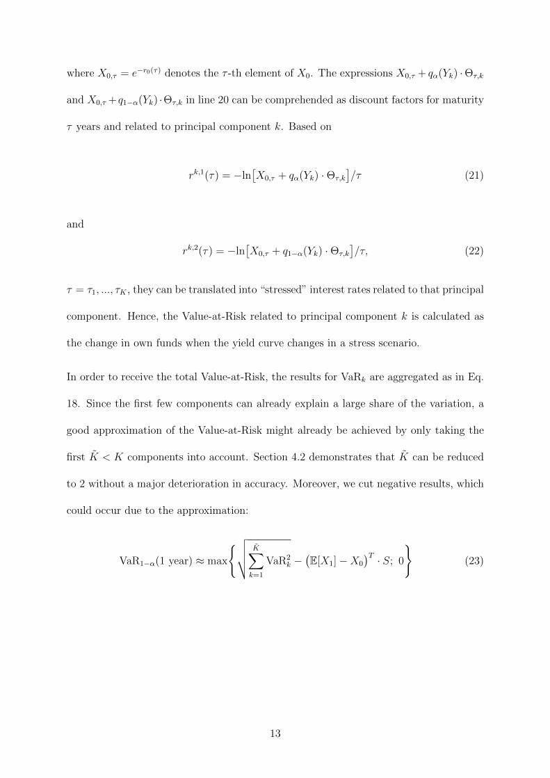
where X0,τ = e−r0(τ) denotes the τ -th element of X0. The expressions X0,τ + qα(Yk) ·Θτ,k

and X0,τ +q1−α(Yk) ·Θτ,k in line 20 can be comprehended as discount factors for maturity

τ years and related to principal component k. Based on

rk,1(τ) = −ln[X0,τ + qα(Yk) ·Θτ,k

]/τ (21)

and

rk,2(τ) = −ln[X0,τ + q1−α(Yk) ·Θτ,k

]/τ, (22)

τ = τ1, ..., τK , they can be translated into “stressed” interest rates related to that principal

component. Hence, the Value-at-Risk related to principal component k is calculated as

the change in own funds when the yield curve changes in a stress scenario.

In order to receive the total Value-at-Risk, the results for VaRk are aggregated as in Eq.

18. Since the first few components can already explain a large share of the variation, a

good approximation of the Value-at-Risk might already be achieved by only taking the

first K < K components into account. Section 4.2 demonstrates that K can be reduced

to 2 without a major deterioration in accuracy. Moreover, we cut negative results, which

could occur due to the approximation:

VaR1−α(1 year) ≈ max

√√√√ K∑k=1

VaR2k −

(E[X1]−X0

)T · S; 0

(23)

13

3 Calibration of interest rate models

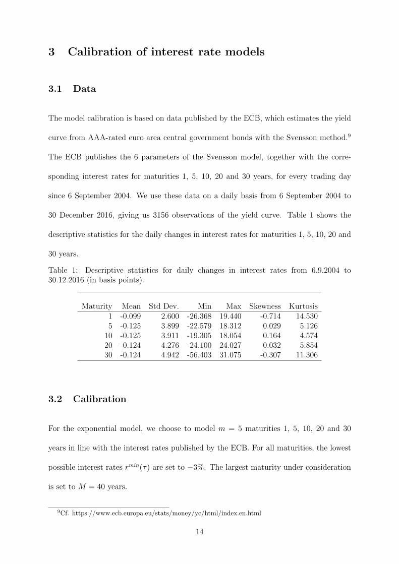
3.1 Data

The model calibration is based on data published by the ECB, which estimates the yield

curve from AAA-rated euro area central government bonds with the Svensson method.9

The ECB publishes the 6 parameters of the Svensson model, together with the corre-

sponding interest rates for maturities 1, 5, 10, 20 and 30 years, for every trading day

since 6 September 2004. We use these data on a daily basis from 6 September 2004 to

30 December 2016, giving us 3156 observations of the yield curve. Table 1 shows the

descriptive statistics for the daily changes in interest rates for maturities 1, 5, 10, 20 and

30 years.

Table 1: Descriptive statistics for daily changes in interest rates from 6.9.2004 to30.12.2016 (in basis points).

Maturity Mean Std Dev. Min Max Skewness Kurtosis1 -0.099 2.600 -26.368 19.440 -0.714 14.5305 -0.125 3.899 -22.579 18.312 0.029 5.126

10 -0.125 3.911 -19.305 18.054 0.164 4.57420 -0.124 4.276 -24.100 24.027 0.032 5.85430 -0.124 4.942 -56.403 31.075 -0.307 11.306

3.2 Calibration

For the exponential model, we choose to model m = 5 maturities 1, 5, 10, 20 and 30

years in line with the interest rates published by the ECB. For all maturities, the lowest

possible interest rates rmin(τ) are set to −3%. The largest maturity under consideration

is set to M = 40 years.

9Cf. https://www.ecb.europa.eu/stats/money/yc/html/index.en.html

14

In the observed time horizon from 2004 to 2016, interest rates have significantly decreased

(cf. column “Mean” in Table 1). We remove this drift from the observed ∆θt-processes

(for the dynamic Svensson model as well as for the exponential model) by deducting the

mean of ∆θ(i)t for each entry i. This helps to avoid the negative drift continuing in the

simulated yield curves of the next year, which would drive interest rates in 1 year below

the current level in expectation.

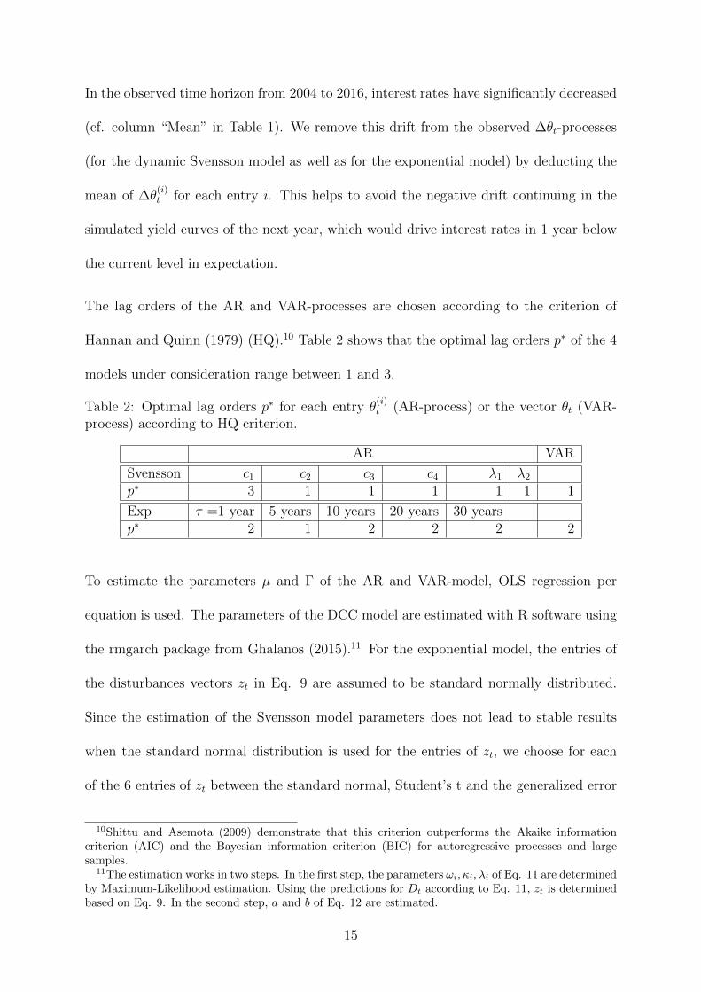
The lag orders of the AR and VAR-processes are chosen according to the criterion of

Hannan and Quinn (1979) (HQ).10 Table 2 shows that the optimal lag orders p∗ of the 4

models under consideration range between 1 and 3.

Table 2: Optimal lag orders p∗ for each entry θ(i)t (AR-process) or the vector θt (VAR-

process) according to HQ criterion.

AR VAR

Svensson c1 c2 c3 c4 λ1 λ2p∗ 3 1 1 1 1 1 1

Exp τ =1 year 5 years 10 years 20 years 30 yearsp∗ 2 1 2 2 2 2

To estimate the parameters µ and Γ of the AR and VAR-model, OLS regression per

equation is used. The parameters of the DCC model are estimated with R software using

the rmgarch package from Ghalanos (2015).11 For the exponential model, the entries of

the disturbances vectors zt in Eq. 9 are assumed to be standard normally distributed.

Since the estimation of the Svensson model parameters does not lead to stable results

when the standard normal distribution is used for the entries of zt, we choose for each

of the 6 entries of zt between the standard normal, Student’s t and the generalized error

10Shittu and Asemota (2009) demonstrate that this criterion outperforms the Akaike informationcriterion (AIC) and the Bayesian information criterion (BIC) for autoregressive processes and largesamples.

11The estimation works in two steps. In the first step, the parameters ωi, κi, λi of Eq. 11 are determinedby Maximum-Likelihood estimation. Using the predictions for Dt according to Eq. 11, zt is determinedbased on Eq. 9. In the second step, a and b of Eq. 12 are estimated.

15

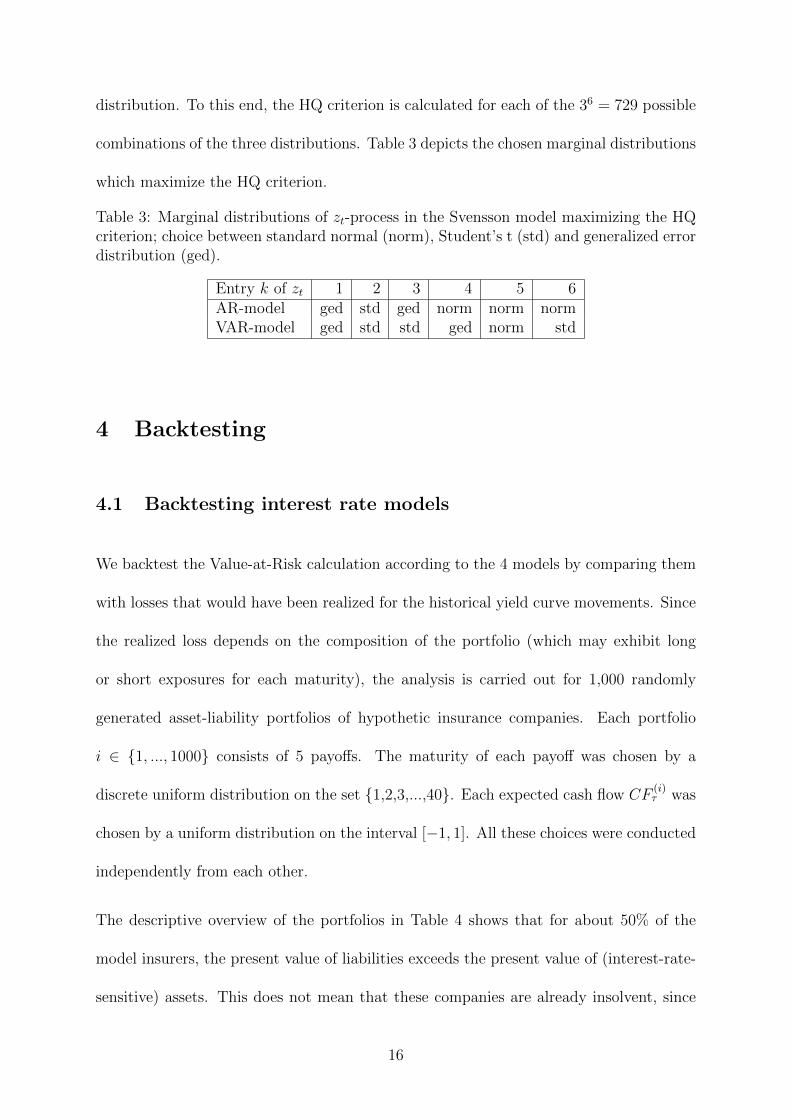
distribution. To this end, the HQ criterion is calculated for each of the 36 = 729 possible

combinations of the three distributions. Table 3 depicts the chosen marginal distributions

which maximize the HQ criterion.

Table 3: Marginal distributions of zt-process in the Svensson model maximizing the HQcriterion; choice between standard normal (norm), Student’s t (std) and generalized errordistribution (ged).

Entry k of zt 1 2 3 4 5 6AR-model ged std ged norm norm normVAR-model ged std std ged norm std

4 Backtesting

4.1 Backtesting interest rate models

We backtest the Value-at-Risk calculation according to the 4 models by comparing them

with losses that would have been realized for the historical yield curve movements. Since

the realized loss depends on the composition of the portfolio (which may exhibit long

or short exposures for each maturity), the analysis is carried out for 1,000 randomly

generated asset-liability portfolios of hypothetic insurance companies. Each portfolio

i ∈ 1, ..., 1000 consists of 5 payoffs. The maturity of each payoff was chosen by a

discrete uniform distribution on the set 1,2,3,...,40. Each expected cash flow CF(i)τ was

chosen by a uniform distribution on the interval [−1, 1]. All these choices were conducted

independently from each other.

The descriptive overview of the portfolios in Table 4 shows that for about 50% of the

model insurers, the present value of liabilities exceeds the present value of (interest-rate-

sensitive) assets. This does not mean that these companies are already insolvent, since

16

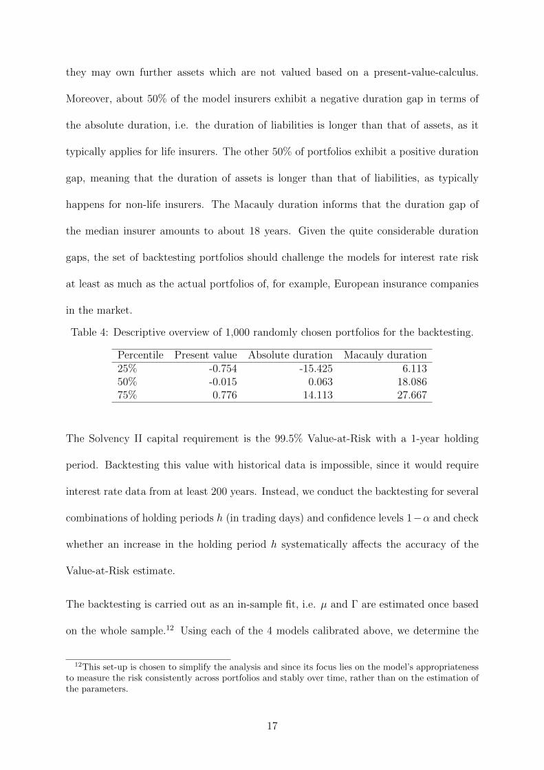
they may own further assets which are not valued based on a present-value-calculus.

Moreover, about 50% of the model insurers exhibit a negative duration gap in terms of

the absolute duration, i.e. the duration of liabilities is longer than that of assets, as it

typically applies for life insurers. The other 50% of portfolios exhibit a positive duration

gap, meaning that the duration of assets is longer than that of liabilities, as typically

happens for non-life insurers. The Macauly duration informs that the duration gap of

the median insurer amounts to about 18 years. Given the quite considerable duration

gaps, the set of backtesting portfolios should challenge the models for interest rate risk

at least as much as the actual portfolios of, for example, European insurance companies

in the market.

Table 4: Descriptive overview of 1,000 randomly chosen portfolios for the backtesting.

Percentile Present value Absolute duration Macauly duration25% -0.754 -15.425 6.11350% -0.015 0.063 18.08675% 0.776 14.113 27.667

The Solvency II capital requirement is the 99.5% Value-at-Risk with a 1-year holding

period. Backtesting this value with historical data is impossible, since it would require

interest rate data from at least 200 years. Instead, we conduct the backtesting for several

combinations of holding periods h (in trading days) and confidence levels 1−α and check

whether an increase in the holding period h systematically affects the accuracy of the

Value-at-Risk estimate.

The backtesting is carried out as an in-sample fit, i.e. µ and Γ are estimated once based

on the whole sample.12 Using each of the 4 models calibrated above, we determine the

12This set-up is chosen to simplify the analysis and since its focus lies on the model’s appropriatenessto measure the risk consistently across portfolios and stably over time, rather than on the estimation ofthe parameters.

17

Value-at-Risk VaRi(1−α),h(t) at day t and for portfolio i. To this end, we generate 5,000

simulations of ηt, ηt+1, ..., ηt+h−1 in accordance with the covariance matrices Ωt, ...,Ωt+h−1.

Then, the parameters θt+1, ..., θt+h (Eq. 7), the interest rates rt+1(τ), , ..., rt+h(τ) (Eq. 4

and 5) and the Value-at-Risk of each portfolio i (Eq. 14) are determined. The Value-at-

Risk VaRi(1−α),h(t) is compared with the historical loss that has occurred for that portfolio

between times t and t+ h:

loss(i)t = −

M∑τ=1

(e−τ ·rt+h(τ) − e−τ ·rt(τ)

)· CF (i)

τ (24)

In order to avoid autocorrelation in the loss(i)t -processes, we conduct this comparison

only beginning at every h-th day of the observed time period. We can thereby observe

n = b3156−3hc pairwise disjunct time windows, each with a length of h days.13 The

percentage of days for which the historical loss exceeds the Value-at-Risk is called the hit

rate:

hit rate =1

n

∑t

1loss(i)t >VaRi(1−α),h(t)(25)

For an accurate Value-at-Risk estimate for portfolio i, the hit rate should be close to α,

i.e. for about α · n days, the historical loss should exceed the Value-at-Risk.

We conduct the analysis for α = 0.5%, α = 5% and α = 10% combined with holding

periods of h = 1, h = 15, h = 30 and h = 50 days. Note that sampling error affects the

hit rate more strongly the smaller α ·n is. Hence, the hit rate of the 99.5% Value-at-Risk

is estimated relatively robustly for h = 1, but it is quite vulnerable to sampling error

13The number of observed realizations of the yield curves is reduced by 3, since we focus on yield curvechanges, and the first 2 observations are needed to kick off the process.

18

when h = 50. For long holding periods, only the hit rate of the 90% Value-at-Risk is

relatively robust.

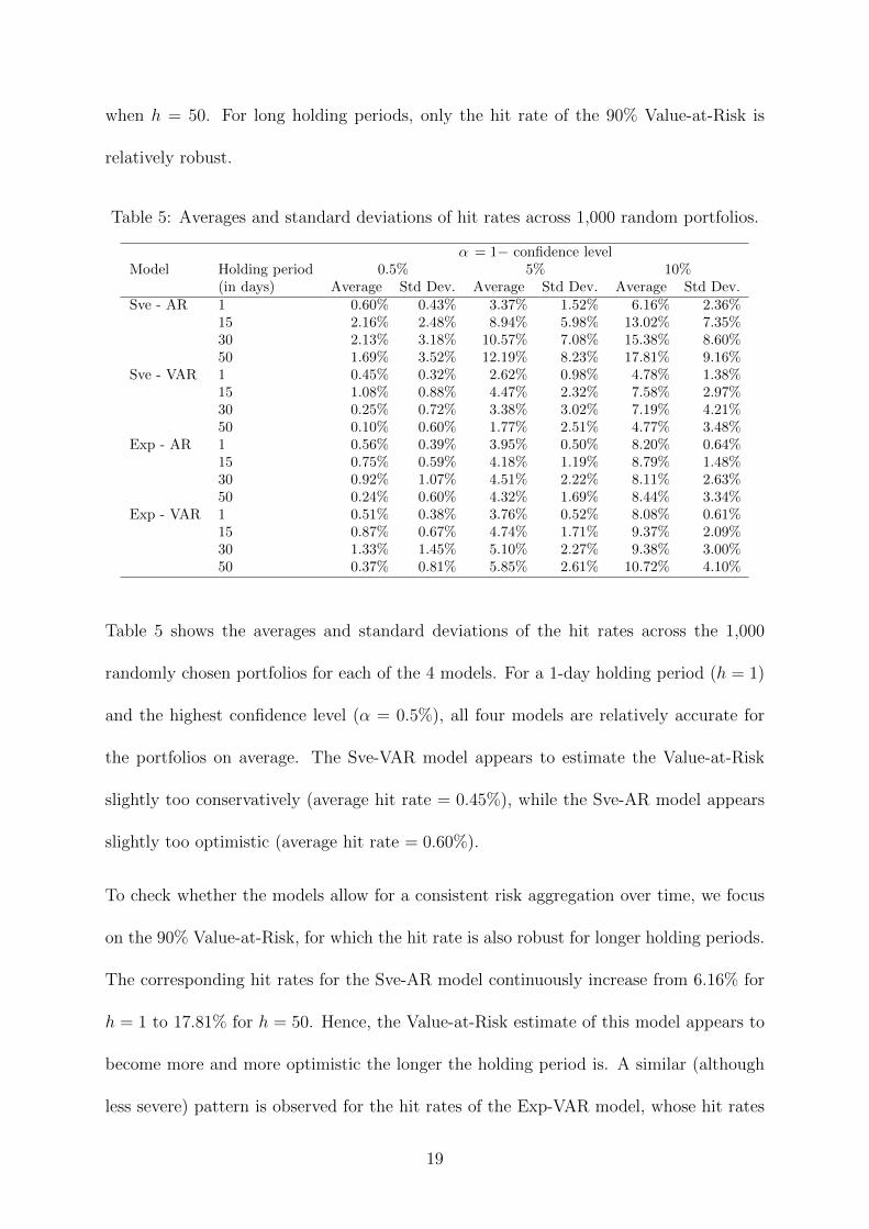
Table 5: Averages and standard deviations of hit rates across 1,000 random portfolios.

α = 1− confidence levelModel Holding period 0.5% 5% 10%

(in days) Average Std Dev. Average Std Dev. Average Std Dev.Sve - AR 1 0.60% 0.43% 3.37% 1.52% 6.16% 2.36%

15 2.16% 2.48% 8.94% 5.98% 13.02% 7.35%30 2.13% 3.18% 10.57% 7.08% 15.38% 8.60%50 1.69% 3.52% 12.19% 8.23% 17.81% 9.16%

Sve - VAR 1 0.45% 0.32% 2.62% 0.98% 4.78% 1.38%15 1.08% 0.88% 4.47% 2.32% 7.58% 2.97%30 0.25% 0.72% 3.38% 3.02% 7.19% 4.21%50 0.10% 0.60% 1.77% 2.51% 4.77% 3.48%

Exp - AR 1 0.56% 0.39% 3.95% 0.50% 8.20% 0.64%15 0.75% 0.59% 4.18% 1.19% 8.79% 1.48%30 0.92% 1.07% 4.51% 2.22% 8.11% 2.63%50 0.24% 0.60% 4.32% 1.69% 8.44% 3.34%

Exp - VAR 1 0.51% 0.38% 3.76% 0.52% 8.08% 0.61%15 0.87% 0.67% 4.74% 1.71% 9.37% 2.09%30 1.33% 1.45% 5.10% 2.27% 9.38% 3.00%50 0.37% 0.81% 5.85% 2.61% 10.72% 4.10%

Table 5 shows the averages and standard deviations of the hit rates across the 1,000

randomly chosen portfolios for each of the 4 models. For a 1-day holding period (h = 1)

and the highest confidence level (α = 0.5%), all four models are relatively accurate for

the portfolios on average. The Sve-VAR model appears to estimate the Value-at-Risk

slightly too conservatively (average hit rate = 0.45%), while the Sve-AR model appears

slightly too optimistic (average hit rate = 0.60%).

To check whether the models allow for a consistent risk aggregation over time, we focus

on the 90% Value-at-Risk, for which the hit rate is also robust for longer holding periods.

The corresponding hit rates for the Sve-AR model continuously increase from 6.16% for

h = 1 to 17.81% for h = 50. Hence, the Value-at-Risk estimate of this model appears to

become more and more optimistic the longer the holding period is. A similar (although

less severe) pattern is observed for the hit rates of the Exp-VAR model, whose hit rates

19

continuously increase from 8.08% to 10.72%. In contrast, the hit rates of the Sve-VAR

model and of the Exp-AR model do not systematically increase or decrease for longer

time periods, in line with a consistent risk aggregation over time.

As explained in the introduction, it is important from a regulatory perspective that the

model’s accuracy is stable across portfolios, which is measured by the variation of hit rates

across the portfolios. Since the standard deviation of the hit rate is systematically higher

the higher the average hit rate is, we focus on the coefficients of variation. From the two

models which consistently aggregate risk over time (Sve-VAR and Exp-AR), the Exp-AR

model exhibits the lower coefficients of variation. For instance, for the 99.5%-Value-at-

Risk, the coefficients of variation of the Exp-AR model amount to 0.39%/0.56% = 69%

for h = 1, 79% for h = 15, 116% for h = 30, and 248% for h = 50. The corresponding

values of the Sve-VAR model amount to 72%, 81%, 294%, and 634%. The Exp-AR model

also exhibits lower coefficients of variation when looking at the hit rates of the 95%-Value-

at-Risk or of the 90%-Value-at-Risk for each of the holding periods considered.

Finally, we demonstrate that the Exp-VAR model performs better than the Sve-VAR

model in terms of the independence of Value-at-Risk exceedances over time. For each

portfolio and each combination of h and α, we employ the independence test of Christof-

fersen (1998) on the null hypothesis that a Value-at-Risk exceedance does not affect the

probability of an exceedance in the subsequent time window. Table 6 shows the portion

of portfolios for which the pattern of Value-at-Risk exceedances is significantly depen-

dent over time with p-values below 1%, 5% and 10%. Regarding the Exp-AR model

for the 99.5%-Value-at-Risk, significant time dependencies occur only for the shortest

holding period of h = 1 day. In this case, for 3.2% of portfolios the exceedances are

time-dependent at a 1% level of significance. For the Sve-VAR model, the corresponding

20

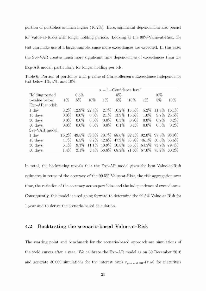
portion of portfolios is much higher (16.2%). Here, significant dependencies also persist

for Value-at-Risks with longer holding periods. Looking at the 90%-Value-at-Risk, the

test can make use of a larger sample, since more exceedances are expected. In this case,

the Sve-VAR creates much more significant time dependencies of exceedances than the

Exp-AR model, particularly for longer holding periods.

Table 6: Portion of portfolios with p-value of Christoffersen’s Exceedance Independencetest below 1%, 5%, and 10%.

α = 1−Confidence levelHolding period 0.5% 5% 10%p-value below 1% 5% 10% 1% 5% 10% 1% 5% 10%Exp-AR model:1 day 3.2% 12.9% 22.4% 2.7% 10.2% 15.5% 5.2% 11.8% 16.1%15 days 0.0% 0.0% 0.0% 2.1% 13.9% 16.6% 1.0% 9.7% 23.5%30 days 0.0% 0.0% 0.0% 0.0% 0.3% 0.9% 0.0% 0.7% 3.2%50 days 0.0% 0.0% 0.0% 0.0% 0.1% 0.1% 0.0% 0.0% 0.2%Sve-VAR model:1 day 16.2% 49.5% 59.8% 70.7% 88.6% 92.1% 92.0% 97.9% 98.9%15 days 4.7% 6.5% 8.7% 42.8% 47.9% 53.9% 46.1% 50.5% 53.6%30 days 6.1% 9.3% 11.1% 40.9% 50.8% 56.3% 64.5% 73.7% 79.4%50 days 1.4% 2.1% 3.4% 58.8% 68.2% 71.8% 67.0% 75.2% 80.2%

In total, the backtesting reveals that the Exp-AR model gives the best Value-at-Risk

estimates in terms of the accuracy of the 99.5% Value-at-Risk, the risk aggregation over

time, the variation of the accuracy across portfolios and the independence of exceedances.

Consequently, this model is used going forward to determine the 99.5% Value-at-Risk for

1 year and to derive the scenario-based calculation.

4.2 Backtesting the scenario-based Value-at-Risk

The starting point and benchmark for the scenario-based approach are simulations of

the yield curves after 1 year. We calibrate the Exp-AR model as on 30 December 2016

and generate 30,000 simulations for the interest rates ryear end 2017(τ, ω) for maturities

21

τ ∈ 1, 5, 10, 20, 30.14 For each simulation path, we fit the parameters of the Svensson

model to the five modeled interest rates.15 Then Eq. 4 is applied to obtain 30,000

simulations of the whole yield curve.

To set up the scenarios, we transform the simulated interest rates ryear end 2017(τ, ω) for

the 5 maturities τ ∈ 1, 5, 10, 20, 30 into principal components (hence, K = 5 in Eq.

15). We then use Eq. 21 and 22 to elicit two stressed yield curves for each principal

component. Each of these scenarios is translated into a complete yield curve by fitting

the Svensson parameters to the 5 stressed interest rates.16 Finally, the Value-at-Risk is

calculated according to Eq. 23.

Table 7 depicts the stressed interest rates for the maturities 1, 5, 10, 20 and 30 years in

terms of absolute changes to the interest rates on 30 December 2016. Regarding the first

principal component (PC1), the two stress scenarios A and B are essentially an upward

and downward shift of interest rates. The second principal component (PC2) affects the

steepness of the yield curve by changing long-term interest rates in a different direction

than short and middle-term rates. At the same time, it impacts the bowing of the yield

curve, since middle-term interest rates are changed more strongly than short and long-

term yields. In terms of the third principal component, only scenario B has an essential

effect on the yield curve. This scenario impacts the curvature, since interest rates for the

maturities 10 and 30 years change in a different direction than those for the others.

We backtest the scenario-based Value-at-Risk by comparing it against the exactly calcu-

lated Value-at-Risk, which is based on the whole simulation. To this end, we generate

14We assume that 1 year has 270 trading days.15As mentioned in section 2.2, we take the values for λ1,t and λ2,t from 30.12.2016 and only fit

c1,t, ..., c4,t by OLS.16Again, λ1,t and λ2,t are taken from 30.12.2016 and c1,t, ..., c4,t are fit by OLS.

22

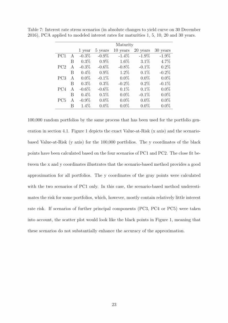
Table 7: Interest rate stress scenarios (in absolute changes to yield curve on 30 December2016), PCA applied to modeled interest rates for maturities 1, 5, 10, 20 and 30 years.

Maturity1 year 5 years 10 years 20 years 30 years

PC1 A -0.3% -0.9% -1.4% -1.9% -1.9%B 0.3% 0.9% 1.6% 3.1% 4.7%

PC2 A -0.3% -0.6% -0.8% -0.1% 0.2%B 0.4% 0.9% 1.2% 0.1% -0.2%

PC3 A 0.0% -0.1% 0.0% 0.0% 0.0%B 0.3% 0.3% -0.2% 0.2% -0.1%

PC4 A -0.6% -0.6% 0.1% 0.1% 0.0%B 0.4% 0.5% 0.0% -0.1% 0.0%

PC5 A -0.9% 0.0% 0.0% 0.0% 0.0%B 1.4% 0.0% 0.0% 0.0% 0.0%

100,000 random portfolios by the same process that has been used for the portfolio gen-

eration in section 4.1. Figure 1 depicts the exact Value-at-Risk (x axis) and the scenario-

based Value-at-Risk (y axis) for the 100,000 portfolios. The y coordinates of the black

points have been calculated based on the four scenarios of PC1 and PC2. The close fit be-

tween the x and y coordinates illustrates that the scenario-based method provides a good

approximation for all portfolios. The y coordinates of the gray points were calculated

with the two scenarios of PC1 only. In this case, the scenario-based method underesti-

mates the risk for some portfolios, which, however, mostly contain relatively little interest

rate risk. If scenarios of further principal components (PC3, PC4 or PC5) were taken

into account, the scatter plot would look like the black points in Figure 1, meaning that

these scenarios do not substantially enhance the accuracy of the approximation.

23

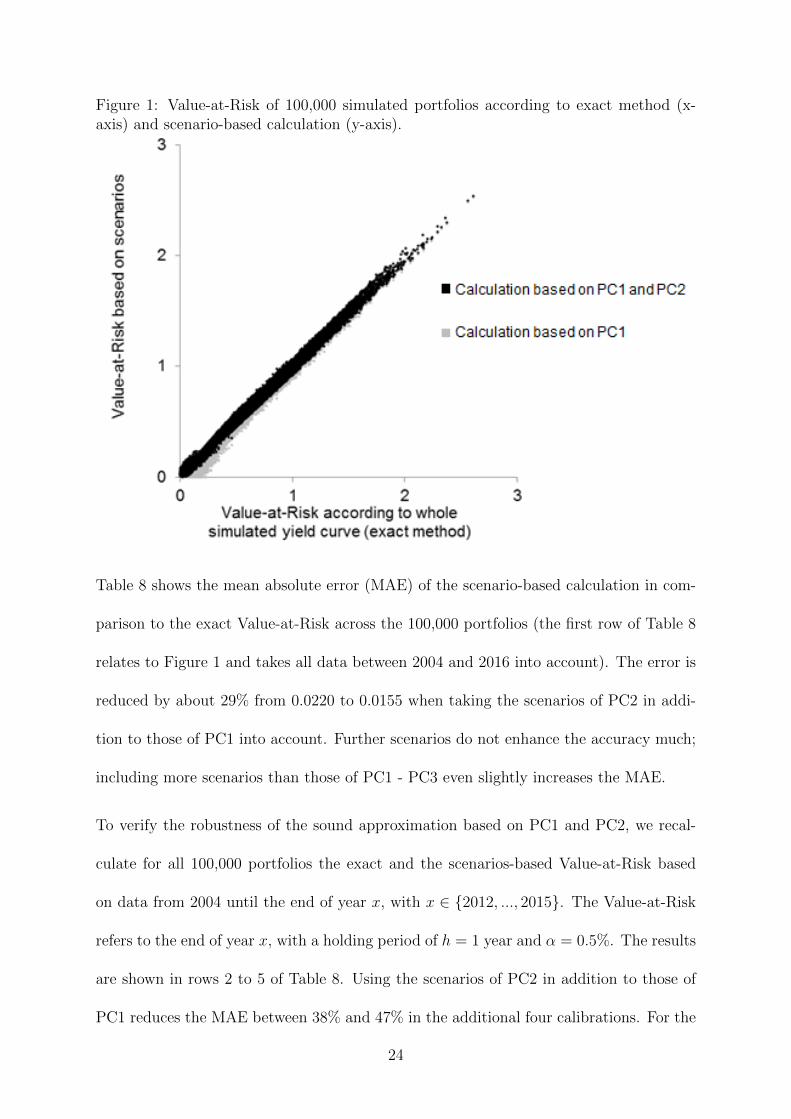
Figure 1: Value-at-Risk of 100,000 simulated portfolios according to exact method (x-axis) and scenario-based calculation (y-axis).

Table 8 shows the mean absolute error (MAE) of the scenario-based calculation in com-

parison to the exact Value-at-Risk across the 100,000 portfolios (the first row of Table 8

relates to Figure 1 and takes all data between 2004 and 2016 into account). The error is

reduced by about 29% from 0.0220 to 0.0155 when taking the scenarios of PC2 in addi-

tion to those of PC1 into account. Further scenarios do not enhance the accuracy much;

including more scenarios than those of PC1 - PC3 even slightly increases the MAE.

To verify the robustness of the sound approximation based on PC1 and PC2, we recal-

culate for all 100,000 portfolios the exact and the scenarios-based Value-at-Risk based

on data from 2004 until the end of year x, with x ∈ 2012, ..., 2015. The Value-at-Risk

refers to the end of year x, with a holding period of h = 1 year and α = 0.5%. The results

are shown in rows 2 to 5 of Table 8. Using the scenarios of PC2 in addition to those of

PC1 reduces the MAE between 38% and 47% in the additional four calibrations. For the

24

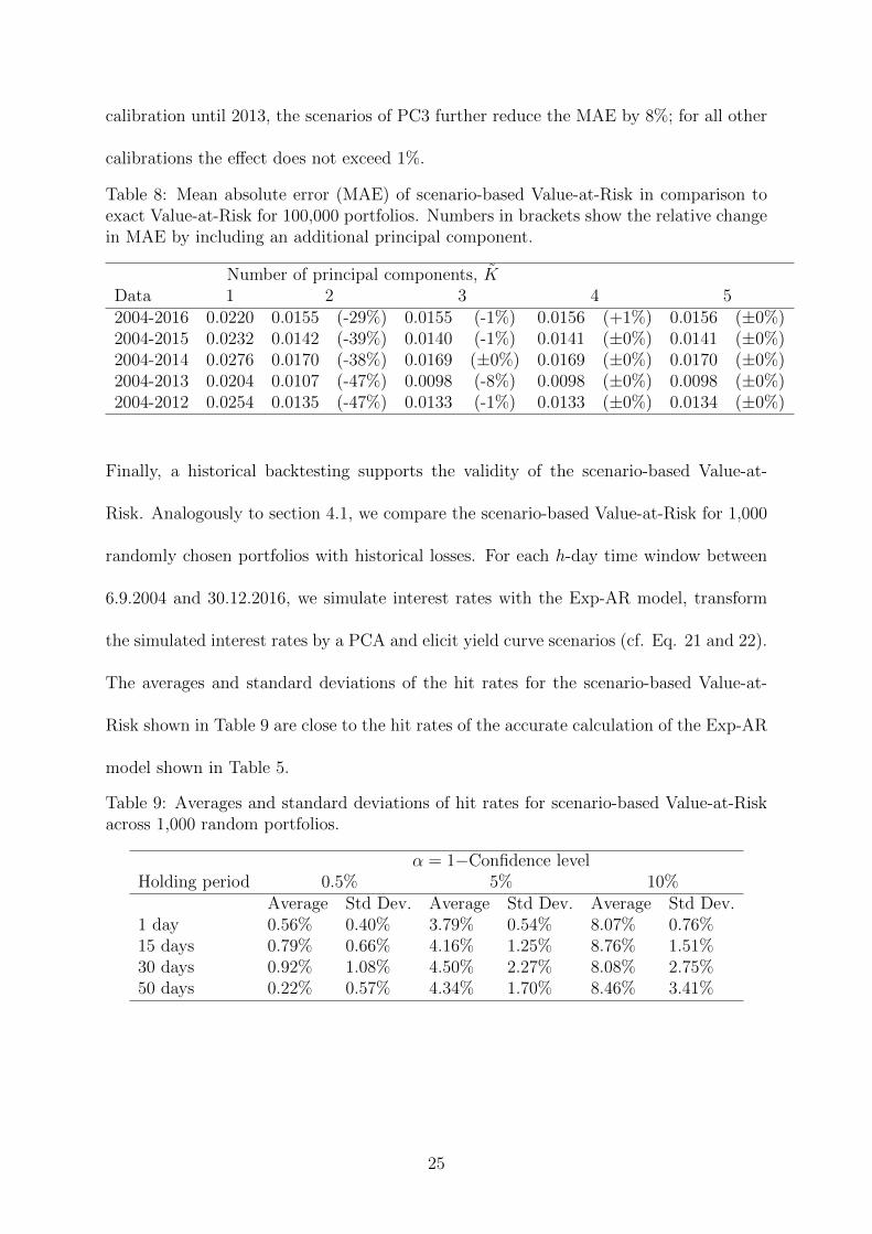
calibration until 2013, the scenarios of PC3 further reduce the MAE by 8%; for all other

calibrations the effect does not exceed 1%.

Table 8: Mean absolute error (MAE) of scenario-based Value-at-Risk in comparison toexact Value-at-Risk for 100,000 portfolios. Numbers in brackets show the relative changein MAE by including an additional principal component.

Number of principal components, KData 1 2 3 4 52004-2016 0.0220 0.0155 (-29%) 0.0155 (-1%) 0.0156 (+1%) 0.0156 (±0%)2004-2015 0.0232 0.0142 (-39%) 0.0140 (-1%) 0.0141 (±0%) 0.0141 (±0%)2004-2014 0.0276 0.0170 (-38%) 0.0169 (±0%) 0.0169 (±0%) 0.0170 (±0%)2004-2013 0.0204 0.0107 (-47%) 0.0098 (-8%) 0.0098 (±0%) 0.0098 (±0%)2004-2012 0.0254 0.0135 (-47%) 0.0133 (-1%) 0.0133 (±0%) 0.0134 (±0%)

Finally, a historical backtesting supports the validity of the scenario-based Value-at-

Risk. Analogously to section 4.1, we compare the scenario-based Value-at-Risk for 1,000

randomly chosen portfolios with historical losses. For each h-day time window between

6.9.2004 and 30.12.2016, we simulate interest rates with the Exp-AR model, transform

the simulated interest rates by a PCA and elicit yield curve scenarios (cf. Eq. 21 and 22).

The averages and standard deviations of the hit rates for the scenario-based Value-at-

Risk shown in Table 9 are close to the hit rates of the accurate calculation of the Exp-AR

model shown in Table 5.

Table 9: Averages and standard deviations of hit rates for scenario-based Value-at-Riskacross 1,000 random portfolios.

α = 1−Confidence levelHolding period 0.5% 5% 10%

Average Std Dev. Average Std Dev. Average Std Dev.1 day 0.56% 0.40% 3.79% 0.54% 8.07% 0.76%15 days 0.79% 0.66% 4.16% 1.25% 8.76% 1.51%30 days 0.92% 1.08% 4.50% 2.27% 8.08% 2.75%50 days 0.22% 0.57% 4.34% 1.70% 8.46% 3.41%

25

5 Conclusion

When determining a method for the definition and monitoring of capital requirements

for financial institutions, regulators traditionally need to deal with a trade-off: on the

one hand, they could force the entities to develop and use an internal model, which

might measure risk appropriately by building on recent market data modeling risks with

Monte-Carlo simulations. However, this requires complex processes on the firms’ side

to implement and maintain the models as well as on the regulator’s side to supervise

the models. On the other hand, capital requirements can be formulated by a pragmatic

standard formula, which, however, typically comes along with mismeasurements which

can create severe disincentives for risk management decisions. This paper suggests a

procedure to translate a Monte-Carlo-based risk measurement of interest rate risk into

a small number of scenarios. The scenarios offer a way to define capital requirements

by a pragmatic calculation rule, the result of which is close to the Monte-Carlo-based

calculation. The suggested procedure utilizes PCA, which is applied to the simulations

of a stochastic model, rather than directly to historical data. By doing so, additional

requirements, such as a lower bound for interest rates, can be included. Apart from the

applicability in the context of a regulatory standard formula, the scenarios can build a

basis for regulatory or enterprise-internal stress tests.17 Moreover, the idea of translating

Monte-Carlo simulations into scenarios could be generally helpful for interpreting and

communicating the results of an interest rate risk model, which is often challenging due

to the large number of simulation paths.

17This is also required in bank risk management, cf. Bank for International Settlements (2016, p.7-10).

26

Further research is needed on the question of how to deal with interest rates for very long

maturities, which cannot be stably estimated from bond market data. Moreover, follow-

up research topics include the integration of further market risks into the scenario-based

approach.

27

References

Bank for International Settlements, 2016. Basel Committee on Banking Supervision.

Standards on Interest rate risk in the banking book.

URL http://www.bis.org/bcbs/publ/d368.htm

Caldeira, J., Moura, G., Santos, A., 2015. Measuring risk in fixed income portfolios using

yield curve models. Computational Economics 46 (1), 65–82.

Christoffersen, P. F., 1998. Evaluating interval forecasts. International Economic Review

39 (4), 841–862.

Diebold, F. X., Li, C., 2006. Forecasting the term structure of government bond yields.

Journal of Econometrics 130 (2), 337–364.

Duffee, G. R., 2002. Term premia and interest rate forecasts in affine models. Journal of

Finance 57 (1), 405–443.

EIOPA, 2014. EIOPA Insurance stress test 2014.

EIOPA, 2016. Discussion Paper on the review of specific items in the Solvency II Dele-

gated Regulation.

Engle, R., 2002. Dynamic conditional correlation: a simple class of multivariate gen-

eralized autoregressive conditional heteroskedasticity models. Journal of Business &

Economic Statistics 20 (3), 339–350.

European Commission, 2009. Directive 2009/138/EC of the European Parliament and

of the Council of 25 November 2009 on the taking-up and pursuit of the business of

Insurance and Reinsurance (Solvency II).

28

Gatzert, N., Martin, M., 2012. Quantifying credit and market risk under solvency ii:

Standard approach versus internal model. Insurance: Mathematics and Economics

51 (3), 649–666.

Ghalanos, A., 2015. rmgarch: Multivariate garch models. r package version 1.3-0.

Hannan, E., Quinn, B., 1979. The determination of the order of an autoregression. Journal

of the Royal Statistical Society, Series B 41 (2), 190–195.

Litterman, R., Scheinkman, J., 1991. Common factors affecting bond returns. The Journal

of Fixed Income 1 (1), 54–61.

Nelson, C. R. N., Siegel, A. F., 1987. Parsimonious modeling of yield curves. The Journal

of Business 60 (4), 473–489.

Shittu, O., Asemota, M., 2009. Comparison of criteria for estimating the order of au-

toregressive process: A monte carlo approach. European Journal of Scientific Research

30 (3), 409–416.

Svensson, L. E. O., 1994. Estimating and interpreting forward interest rates: Sweden

1992-1994. IMF Working Papers 94/114.

29