Scattering Theory of Molecules, Atoms and Nuclei || Green's Functions, T- and S-Matrices

September 21, 2012 15:54 8012 - Scattering Theory of Molecules, Atoms and Nuclei canto-hussein

Chapter 4

Green’s Functions, T- and S-Matrices

The previous two chapters were devoted to the partial-wave expansion

method in scattering theory. Here, we discuss a new approach: the Green’s

function method. This method leads to the Lippmann-Schwinger equations,

which have integro-differencial form in the coordinate representation. Al-

though exact solutions of these equations are very hard to find, they are

suitable for the derivation of perturbative approximations. In the discus-

sion of the Lippmann-Schwinger equations, we introduce the concepts of

Green’s functions, Møller operators and the S- and the T-matrices, which

play very important roles in scattering theory.

Since we have shown (see chapter 1) that the realistic time-dependent

wave-packet treatment of the scattering problem is equivalent to the sta-

tionary diffusion of a plane wave, we base most of the present chapter on

the simpler time-independent approach. In most situations one deals with

real potentials, which leads to a series of important properties. However,

sometimes one uses complex potentials to simulate coupled-channel effects

on the elastic channel. Throughout this chapter, we assume that the in-

teraction potential is real and spherically symmetric. The scattering from

complex potentials will be discussed in chapters 7 and 10.

4.1 Lippmann-Schwinger equations

We start with the Schrodinger equations for a free particle with wave vector

k and energy Ek ≡ Ek = ~2k2/2µ, and the corresponding equation when

this particle is submitted to the action of a short-range potential, which

vanishes for r > R. Using Dirac’s notation, we can write

(Ek −H0) |φ (k)〉 = 0 (4.1)

107

Sca

tteri

ng T

heor

y of

Mol

ecul

es, A

tom

s an

d N

ucle

i Dow

nloa

ded

from

ww

w.w

orld

scie

ntif

ic.c

omby

NA

TIO

NA

L U

NIV

ER

SIT

Y O

F SI

NG

APO

RE

on

05/2

6/14

. For

per

sona

l use

onl

y.


108 Scattering Theory of Molecules, Atoms and Nuclei

and

(Ek −H) |ψ (k)〉 = 0. (4.2)

Above, H0 = K is the kinetic energy operator and H = H0 + V. Since

H†0 = H0 and H† = H, the states |φ (k)〉 and |ψ (k)〉 can be normalized so

as to satisfy the relations

〈φ (k′)|φ (k)〉 = δ (k− k′) , (4.3)

and

〈ψ (k′)|ψ (k)〉 = δ (k− k′) (4.4a)

〈ψm|ψ (k)〉 = 0 (4.4b)

〈ψm|ψn〉 = δmn. (4.4c)

Above, m and n stand for negative energy states which the Hamiltonian

H may possibly have, and δmn and δ (k− k′) are respectively the usual

Kronecker’s and Dirac’s deltas. The identity operator in the Hilbert spaces

spanned by |φ (k)〉 and |ψ (k)〉 can be written∫|φ (k)〉 d3k 〈φ (k)| = 1 (4.5)

and ∫|ψ (k)〉 d3k 〈ψ (k)| +

∑n

|ψn〉〈ψn| = 1 . (4.6)

The free particle’s and the full Green’s operators are respectively de-

fined as,

G0(E) =1

E −H0(4.7)

G(E) =1

E −H. (4.8)

To find a relation between G and G0, we use the operator identity

A−1 = B−1 +B−1(B −A)A−1.

Setting A = E −H ≡ E − (H0 + V ) and B = E −H0, we get

G(E) = G0(E) +G0(E)V G(E), (4.9)

or, setting A = E −H0 and B = E − (H0 + V ), we get

G(E) = G0(E) +G(E)V G0(E). (4.10)

Sca

tteri

ng T

heor

y of

Mol

ecul

es, A

tom

s an

d N

ucle

i Dow

nloa

ded

from

ww

w.w

orld

scie

ntif

ic.c

omby

NA

TIO

NA

L U

NIV

ER

SIT

Y O

F SI

NG

APO

RE

on

05/2

6/14

. For

per

sona

l use

onl

y.


Green’s Functions, T- and S-Matrices 109

The state |ψ (k)〉 satisfies equations involving the Green’s operators. To

derive these equations, we put Eq. (4.2) in the form

(E −H0) |ψ (k)〉 = V |ψ (k)〉 (4.11)

and write |ψ (k)〉 as the sum of the incident and the scattered waves,

|ψ (k)〉 = |φ (k)〉 + |ψsc (k)〉 . (4.12)

Inserting Eq. (4.12) into Eq. (4.11) and using Eq. (4.1), we obtain

(Ek −H0) |ψsc (k)〉 = V |ψ (k)〉 . (4.13)

Multiplying from the left with G0(E) and replacing |ψsc (k)〉 = |ψ (k)〉 −|φ (k)〉, we get the desired equation,

|ψ (k)〉 = |φ (k)〉 + G0(Ek)V |ψ (k)〉 . (4.14)

A similar equation can be obtained in terms of the full Green’s function.

For this purpose, we use Eq. (4.12) in the RHS of Eq. (4.13) and re-arrange

the equation in the form

(Ek −H0 − V ) |ψsc〉 = V |ψ (k)〉 .

Multiplying from the left with G(Ek) we get

|ψsc〉 = G(Ek)V |φ (k)〉 .

Adding |φ (k)〉 to both sides of the above equation and using Eq. (4.12), we

obtain

|ψ (k)〉 = |φ (k)〉 + G(Ek)V |φ (k)〉 = (1 +G(Ek)V ) |φ (k)〉 . (4.15)

Eqs. (4.14) and (4.15) are usually called Lippmann-Schwinger (LS) equa-

tions.

4.1.1 The free particle Green’s function

We now evaluate the matrix elements of the free Green’s operator in the

coordinate representation, called the free-particle Green’s Function. We

start from the spectral decomposition of G0,

G0(Ek) ≡∫d3q

|φ (q)〉〈φ (q)|Ek − Eq

(4.16)

= −(

2µ

~2

) ∫d3q|φ (q)〉〈φ (q)|

q2 − k2,

Sca

tteri

ng T

heor

y of

Mol

ecul

es, A

tom

s an

d N

ucle

i Dow

nloa

ded

from

ww

w.w

orld

scie

ntif

ic.c

omby

NA

TIO

NA

L U

NIV

ER

SIT

Y O

F SI

NG

APO

RE

on

05/2

6/14

. For

per

sona

l use

onl

y.



and take matrix elements in the coordinate representation. We get

G0(Ek; r, r′) = −(

2µ

~2

) ∫d3q

φ(q; r) φ∗ (q; r′)

q2 − k2. (4.17)

Next, we use the normalized free particle’s wave functions

φ(q; r) =1

(2π)3/2

eiq·r; φ∗(q; r′) =1

(2π)3/2

e−iq·r′, (4.18)

introduce the notation

R = r− r′,

and evaluate the integral over q in spherical coordinates, with the z-axis

along the R-direction. Owing to the axial symmetry, the integration over

the azimuthal angle produces the trivial factor 2π and we get1

G0(Ek; r, r′) = −(

2µ

~2

)1

(2π)2

∫q2 dq

q2 − k2

∫ 1

−1

d (cos θq) eiqR cos θq ,

(4.19)

where θq is the angle between the vectors q and R. Performing the inte-

gration over θq, the above integral takes the form

G0(Ek; r, r′) =

(2µ

~2

)i

(2π)2R

(I1 + I2) , (4.20)

with

I1 =

∫ ∞0

dqq eiqR

q2 − k2and I2 = −

∫ ∞0

dqq e−iqR

q2 − k2. (4.21)

Changing q → −q, the second integral in Eq. (4.21) becomes

I2 =

∫ 0

−∞dq

q eiqR

q2 − k2,

so that

I1 + I2 =

∫ ∞−∞

dqq eiqR

q2 − k2. (4.22)

Using Eq. (4.22) and the identity

q

q2 − k2=

1

2

[1

q − k+

1

q + k

]in Eq. (4.20), we get

G0(Ek; r, r′) =

(2µ

~2

)i

2 (2π)2R

∫ ∞−∞

dq

[1

q − k+

1

q + k

]eiqR. (4.23)

1The fact that the Green’s function depends on r and r′ only through the distance

R = |r− r′| is a consequence of the translational and rotational invariances of H0.

Sca

tteri

ng T

heor

y of

Mol

ecul

es, A

tom

s an

d N

ucle

i Dow

nloa

ded

from

ww

w.w

orld

scie

ntif

ic.c

omby

NA

TIO

NA

L U

NIV

ER

SIT

Y O

F SI

NG

APO

RE

on

05/2

6/14

. For

per

sona

l use

onl

y.



The above integral is not defined owing to the poles of the integrand

at q = ± k. However, meaningful Green’s functions G(+)

0 (Ek; r, r′) and

G(−)

0 (Ek; r, r′) can be obtained moving the poles into the complex-plane,

up or down the real axis, according to the prescriptions,

±k → ± (k + i ε′) (G0(Ek; r, r′)→ G(+)

0 (Ek; r, r′)) (4.24)

and

±k → ± (k − i ε′) (G0(Ek; r, r′)→ G(−)

0 (Ek; r, r′)). (4.25)

These procedures correspond to redefining the Green’s operator as

G0(Ek) −→ G(±)

0 (Ek) = limε→0

[1

Ek −H0 ± i ε

], (4.26)

where ε =(~2k/µ

)ε′ is an infinitesimal quantity. It is equivalent to the

analytical continuation of the variable Ek onto the complex plane, where it

takes the values Ek ± i ε. In a similar way, for the full interacting Green’s

function, we define

G(±)(Ek) = limε→0

[1

Ek −H ± i ε

]. (4.27)

It can be easily checked that the matrix-elements of the free and the

full Green’s operators in the coordinate representation, G(±)

0 (Ek; r, r′) and

G(±) (Ek; r, r′) , respectively satisfy the equations[Ek +

~2

2µO2

r

]G(±)

0 (Ek; r, r′) = δ (r− r′) (4.28)

and [Ek +

~2

2µO2

r − V (r)

]G(±) (Ek; r, r′) = δ (r− r′) . (4.29)

Eqs. (4.26) and (4.27), together with the hermiticity of the Hamiltoni-

ans, lead to the properties[G(±)

0 (Ek)]†

= G(∓)0 (Ek) (4.30)

[G(±)(Ek)]†

= G(∓)(Ek) . (4.31)

Using the standard result (see, e.g., [Rodberg and Thaler (1967)])

limε→0

[1

x± iε

]= P

(1

x

)∓ iπ δ(x) , (4.32)

where P stands for the Cauchy’s principal value, G(±)0 (Ek) is split as

G(±)

0 (Ek) = P(

1

Ek −H0

)∓ iπ δ(Ek −H0) . (4.33)

Sca

tteri

ng T

heor

y of

Mol

ecul

es, A

tom

s an

d N

ucle

i Dow

nloa

ded

from

ww

w.w

orld

scie

ntif

ic.c

omby

NA

TIO

NA

L U

NIV

ER

SIT

Y O

F SI

NG

APO

RE

on

05/2

6/14

. For

per

sona

l use

onl

y.



Re k

Im

k

D

Γ(b)

Re k

Im

k

D

Γ(a)

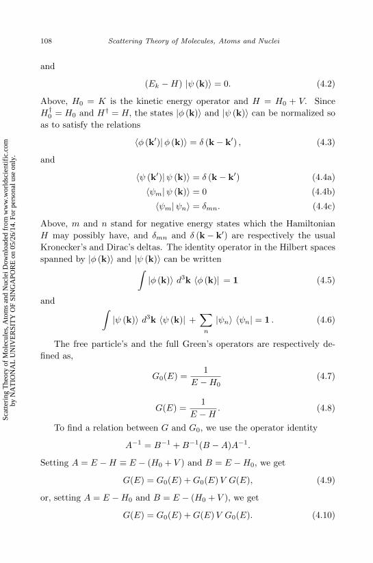
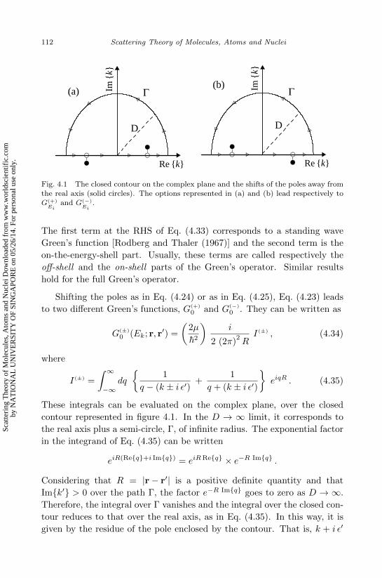
Fig. 4.1 The closed contour on the complex plane and the shifts of the poles away from

the real axis (solid circles). The options represented in (a) and (b) lead respectively toG(+)Ei

and G(−)Ei

.

The first term at the RHS of Eq. (4.33) corresponds to a standing wave

Green’s function [Rodberg and Thaler (1967)] and the second term is the

on-the-energy-shell part. Usually, these terms are called respectively the

off-shell and the on-shell parts of the Green’s operator. Similar results

hold for the full Green’s operator.

Shifting the poles as in Eq. (4.24) or as in Eq. (4.25), Eq. (4.23) leads

to two different Green’s functions, G(+)

0 and G(−)

0 . They can be written as

G(±)

0 (Ek; r, r′) =

(2µ

~2

)i

2 (2π)2RI(±) , (4.34)

where

I(±) =

∫ ∞−∞

dq

1

q − (k ± i ε′)+

1

q + (k ± i ε′)

eiqR . (4.35)

These integrals can be evaluated on the complex plane, over the closed

contour represented in figure 4.1. In the D → ∞ limit, it corresponds to

the real axis plus a semi-circle, Γ, of infinite radius. The exponential factor

in the integrand of Eq. (4.35) can be written

eiR(Req+i Imq) = eiRReq × e−R Imq .

Considering that R = |r− r′| is a positive definite quantity and that

Imk′ > 0 over the path Γ, the factor e−R Imq goes to zero as D → ∞.

Therefore, the integral over Γ vanishes and the integral over the closed con-

tour reduces to that over the real axis, as in Eq. (4.35). In this way, it is

given by the residue of the pole enclosed by the contour. That is, k + i ε′

Sca

tteri

ng T

heor

y of

Mol

ecul

es, A

tom

s an

d N

ucle

i Dow

nloa

ded

from

ww

w.w

orld

scie

ntif

ic.c

omby

NA

TIO

NA

L U

NIV

ER

SIT

Y O

F SI

NG

APO

RE

on

05/2

6/14

. For

per

sona

l use

onl

y.



for I(+) and − (k − i ε′) for I(−). Taking the contour in the counterclockwise

sense, we get

I(±) = 2πi× Res q = ± (k ± i ε′) = 2πi e±ikR . (4.36)

Inserting Eq. (4.36) into Eq. (4.34) and replacing R = |r− r′|, we obtain

the free particle Green’s function:

G(±)

0 (Ek; r, r′) = −(

2µ

~2

)1

4π

e± ik |r−r′|

|r− r′|. (4.37)

We remark that some authors write the free particle’s Green’s function

without the factor within round brackets at the RHS of Eq. (4.37). This

happens when the starting equation is written in the form[∇2 + k2

] ∣∣ψ (k)⟩

= U∣∣ψ (k)

⟩,

with U = 2µV/~2. In this case, the Green’s function is defined as

G(±)

0 (Ek) =(∇2 + k2

)−1. Following the same procedures as above, one gets

Eq. (4.37) but without the factor 2µ/~2. However, the resulting Lippmann-

Schwinger equation is unaffected since the potential V must be replaced by

U and in this way the factor 2µ/~2 is recovered.

A practical consequence of the above discussion is that different wave

functions are generated by the Green’s functions G(+)

0 and G(−)

0 . One should

distinguish the states |ψ(+) (k)〉 and |ψ(−) (k)〉, given by the Lippmann-

Schwinger equations

|ψ(±) (k)〉 = |φ (k)〉 + G(±)0 (Ek)V |ψ(±) (k)〉 . (4.38)

This point will be further discussed in the next section.

Equivalent Lippmann-Schwinger equations are generated by the full

Green’s functions G(±)(Ek), namely

|ψ(±) (k)〉 = |φ (k)〉 + G(±)(Ek)V |φ (k)〉 ≡ (1 +G(±)(Ek)V ) |φ (k)〉 .(4.39)

4.1.2 The scattering amplitude

Although ψ(+) (k) and ψ(−) (k) are solutions of the same equation with the

same energy, they have different boundary conditions. To clarify this point,

we evaluate the asymptotic forms of these wave functions. In the coordinate

representation, the Lippmann-Schwinger equations are written2

ψ(±) (k; r) =φ (k; r) +

∫d3r′G(±)

0 (Ek; r, r′) V (r′) ψ(±)(k; r′

)(4.40)

2Here, we are assuming the locality of the potential V . Non-local potentials will be

discussed in section 4.4.

Sca

tteri

ng T

heor

y of

Mol

ecul

es, A

tom

s an

d N

ucle

i Dow

nloa

ded

from

ww

w.w

orld

scie

ntif

ic.c

omby

NA

TIO

NA

L U

NIV

ER

SIT

Y O

F SI

NG

APO

RE

on

05/2

6/14

. For

per

sona

l use

onl

y.



or, using the Eq. (4.37),

ψ(±) (k; r) = φ (k; r) − 2µ

4π~2

∫d3r′

e± ik |r−r′|

|r− r′|V (r′) ψ(±)

(k; r′

). (4.41)

We now take the |r| → ∞ limit. Since V vanishes when r′ is outside the

potential range (|r′| > R), |r′| / |r| → 0 and one can replace

1

|r− r′|→ 1

r. (4.42)

The factor exp (± ik |r− r′|) must be handled more carefully. It is neces-

sary to expand to first order in r′/r,

k |r− r′| ≡ k(r2 + r′ 2 − 2 r · r′

)1/2 ' kr − k r · r′.

Accordingly, the exponential factor is approximated as

e±ik |r−r′| = e± ikr × e∓ ik r·r′ , (4.43)

where r is the unit vector along r. Inserting Eqs. (4.42) and (4.43) into

Eq. (4.41) and defining the final wave vector q = k r, we obtain

ψ(±) (k; r)→ φ(k; r) +e±ikr

r

(− 2µ

4π~2

∫d3r′ e∓ iq ·r

′V (r′) ψ(±)

(k; r′

)).

Using Eq. (4.18), and switching to Dirac’s notation, the above equation

becomes

ψ(±) (k; r)→ 1

(2π)3/2

[eik·r +

e±ikr

r

(− 2π2

(2µ

~2

)⟨φ (±q)

∣∣V ∣∣ψ(±) (k)⟩)]

.

(4.44)

Inspecting the above equation for ψ(+), we conclude that the Green’s func-

tion G(+)

0 (Ek; r, r′) generates a state which asymptotically behaves as the

sum of the incident plane wave with an outgoing spherical wave. This is

the desired scattering solution. A comparison with Eq. (2.3) (with the

normalization constant A = (2π)−3/2

) leads to the relation

f(θ) = −2π2

(2µ

~2

) ⟨φ (q)

∣∣∣V ∣∣∣ψ(+) (k)⟩. (4.45)

Above, θ is the observation angle which corresponds to the angle between

the initial (k) and the final (q) wave vectors. The meaning of the solution

generated by G(−)

0 (Ek; r, r′) is not straightforward. However, it is very

useful for calculations, as will be discussed later in this chapter.

Sca

tteri

ng T

heor

y of

Mol

ecul

es, A

tom

s an

d N

ucle

i Dow

nloa

ded

from

ww

w.w

orld

scie

ntif

ic.c

omby

NA

TIO

NA

L U

NIV

ER

SIT

Y O

F SI

NG

APO

RE

on

05/2

6/14

. For

per

sona

l use

onl

y.



4.1.3 Orthonormality relation for scattering states

Since the solutions |ψ(+)〉 have the same boundary condition, they form an

orthonormal set. The set of states |ψ(−)〉 have the same property. The

orthonormalization relations of Eqs. (4.4a) and (4.4c) should then be re-

written as

〈ψ(±) (k′) |ψ(±) (k)〉 = δ (k− k′) , (4.46)

〈ψm|ψ(±) (k)〉 = 0, (4.47)

〈ψm|ψn〉 = δm,n. (4.48)

These orthonormality relations can be formally derived from the Lippmann-

Schwinger equations. Let us, for example, evaluate the scalar product

of Eq. (4.46) in the case of outgoing states. We first use the Hermitian

conjugate version of the Lippmann-Schwinger equation (Eq. (4.39)) for

|ψ(+) (k′)〉, writing the explicit form of the full Green’s function (Eq. (4.27)).

We get

〈ψ(+) (k′) |ψ(+) (k)〉 = 〈φ (k′)|ψ(+) (k)〉

+⟨φ (k′)

∣∣∣V 1

Ek′ −H − iε

∣∣∣ψ(+) (k)⟩. (4.49)

Applying the operator (Ek′ −H + iε)−1

on |ψ(+) (k)〉 in the second term

on the RHS of Eq. (4.49) we obtain

〈ψ(+) (k′) |ψ(+) (k)〉 = 〈φ (k′)|ψ(+) (k)〉

+1

Ek′ − Ek − iε

⟨φ (k′)

∣∣∣V ∣∣∣ψ(+) (k)⟩.

Now, we use Eq. (4.38) for |ψ(+) (k)〉 in the first term on the RHS of the

above equation and it becomes

〈ψ(+) (k′) |ψ(+) (k)〉 = 〈φ (k′)|φ (k)〉 +⟨φ (k′)

∣∣∣ 1

Ek −H0 + iεV∣∣∣ψ(+) (k)

⟩+

1

Ek′ − Ek − iε

⟨φ (k′)

∣∣∣V ∣∣∣ψ(+) (k)⟩. (4.50)

Letting the operator (Ek −H0 + iε)−1

act on the bra state 〈φ (k′)|, the

second term on the RHS of Eq. (4.50) exactly cancels the third. The above

equation is then reduced to

〈ψ(+) (k′) |ψ(+) (k)〉 = 〈φ (k′)|φ (k)〉. (4.51)

Since our free states form an orthonormal set, Eq. (4.46) is proved. An

analogous proof can be carried out for the estates |ψ(−) (k)〉 .

Sca

tteri

ng T

heor

y of

Mol

ecul

es, A

tom

s an

d N

ucle

i Dow

nloa

ded

from

ww

w.w

orld

scie

ntif

ic.c

omby

NA

TIO

NA

L U

NIV

ER

SIT

Y O

F SI

NG

APO

RE

on

05/2

6/14

. For

per

sona

l use

onl

y.



4.1.4 The Møller wave operators

It is convenient to introduce the Møller wave operators, Ω(±), which trans-

form free waves into scattering states. That is,

Ω(±) |φ (k)〉 = |ψ(±) (k)〉 . (4.52)

These operators are a very useful tool in the derivation of formal expressions

in scattering theory. Inserting Eq. (4.52) into Eq. (4.38) we obtain

Ω(±) |φ (k)〉 =[1 +G(±)

0 (Ek) V Ω(±)]|φ (k)〉 .

This equation means that the operators Ω(±), or equivalently[1 +G(±)

0 (Ek) V Ω(±)], transform a free state with energy Ek into the scat-

tering state with the same energy. This can be expressed by the Lippmann-

Schwinger equation

Ω(±) (Ek) = 1 +G(±)

0 (Ek) V Ω(±) (Ek) . (4.53)

We emphasize that the Møller wave operators, as defined in Eq. (4.52)

and also in the forthcoming Eq. (4.101), are energy-independent. However,

their Lippmann-Schwinger equations only hold in the space of states with

the energy appearing in the argument of the Green’s function, Ek. To

emphasize this point, we use the notation Ω(±) (Ek) . A similar equation in

terms of G(±) (Ek) can be derived. Comparing Eqs. (4.52) and (4.39) we

get

Ω(±) (Ek) = 1 + G(±) (Ek) V. (4.54)

It can easily be checked that the operators Ω(±) have the properties:

Ω(±) =

∫d3k |ψ(±) (k)〉〈φ (k)| . (4.55)

Ω(±)† Ω(±) = 1 , (4.56)

Ω(±) Ω(±)† = 1−∑n

|ψn〉〈ψn| . (4.57)

Several useful identities involving the Møller operators can be readily de-

rived. We have

Ω(±)† = 1 + Ω(±)†V G(±)†0 = 1 + Ω(±)†V G(∓)

0 , (4.58)

which can be solved for Ω(±)† and Ω(±), with the results

Ω(±)† =1

1− V G(∓)

0

(4.59)

Ω(±) =1

1−G(±)

0 V. (4.60)

Sca

tteri

ng T

heor

y of

Mol

ecul

es, A

tom

s an

d N

ucle

i Dow

nloa

ded

from

ww

w.w

orld

scie

ntif

ic.c

omby

NA

TIO

NA

L U

NIV

ER

SIT

Y O

F SI

NG

APO

RE

on

05/2

6/14

. For

per

sona

l use

onl

y.



4.2 The transition and the scattering operators

Eq. (4.45) indicates that the scattering amplitude is proportional to the

matrix-element of the potential between a final free state with wave vector

along the observation direction, and the full scattering state. However,

these states do not belong to the same orthogonal set. Thus, it is convenient

to use the operator Ω(±) to express the scattering amplitude in terms of

matrix-elements between free states with the initial and the final wave

vectors. Using Eq. (4.52), we obtain

f(θ) = −2π2

(2µ

~2

) ⟨φ (k′)

∣∣∣V Ω(+)

∣∣∣φ (k)⟩. (4.61)

The transition operator is defined as

T = V Ω(+). (4.62)

The set of matrix-elements of T between free states, represented as

Tk′,k ≡ 〈φ (k′)|T |φ (k)〉 = 〈φ (k′)|V Ω(+) |φ (k)〉

=⟨φ (k′)

∣∣∣V ∣∣∣ψ(+) (k)⟩, (4.63)

is called the T-matrix. Its matrix-elements on-the-energy-shell, i.e. with

|k′| = |k| , give the probability amplitude for the transition from the in-

cident momentum ~k to the final momentum ~k′, through the action of

the potential V . Thus, in the absence of potential the transition matrix

vanishes identically. Inserting Eq. (4.63) into Eq. (4.45), the scattering

amplitude becomes3

f(θ) = −2π2

(2µ

~2

)Tk′,k. (4.64)

Therefore, the T-matrix elements lead directly to the scattering amplitude

and give the cross section.

Eq. (4.63) is frequently written as a power series. Using recursively the

Lippmann-Schwinger equation for |ψ(+) (k)〉 (Eq. (4.38)), we get

Tk′,k =

⟨φ (k′)

∣∣∣∣∣V∞∑n=0

(G(+)

0 (Ek)V)n ∣∣∣∣∣φ (k)

⟩. (4.65)

3Note that the constant of proportionality between the scattering amplitude and theT-matrix depends on the choice of the normalization of the plane wave. We use A =(2π)−3/2 and obtain −2π2

(2µ/~2

). Some authors (like Austern in [Austern (1970)])

use A = 1. In this case it takes the value −µ/2π~2.

Sca

tteri

ng T

heor

y of

Mol

ecul

es, A

tom

s an

d N

ucle

i Dow

nloa

ded

from

ww

w.w

orld

scie

ntif

ic.c

omby

NA

TIO

NA

L U

NIV

ER

SIT

Y O

F SI

NG

APO

RE

on

05/2

6/14

. For

per

sona

l use

onl

y.



Replacing G(+)

0 (Ek) by its spectral representation (Eq. (4.16)), we obtain

Tk′,k = 〈φ (k′)|V |φ (k)〉+

∫d3q〈φ (k′)|V |φ (q)〉〈φ (q)|V |φ (k)〉

Ek − Eq + iε

+

∫d3q d3q′

〈φ (k′)|V |φ (q)〉〈φ (q)|V |φ (q′)〉〈φ (q′)|V |φ (k)〉(Ek − Eq + iε) (Ek − Eq′ + iε)

+ · · · higher order terms. (4.66)

Eq. (4.65) (or equivalently Eq. (4.66)) is known as the Born’s series. Ne-

glecting in Eq.(4.65) terms beyond n = 0 (i.e. truncating the series of

Eq. (4.66) after the first term) is the first order Born approximation, or

simply the Born approximation. It will be discussed in detail in chapter 5.

Multiplying Eq. (4.53) (for the outgoing boundary condition) from the

left by V and using Eq. (4.62), we get the Lippmann-Schwinger equation

for the transition operator,

T = V + V G(+)

0 (Ek)T. (4.67)

Using the same procedure for Eq. (4.54), we obtain the equivalent equation

T = V + V G(+)(Ek)V. (4.68)

If one writes Eqs. (4.67) and (4.68) in the momentum representation,

both on-the-energy-shell and off-the-energy-shell matrix-elements must

be considered. That is, the on-the-energy-shell matrix-elements Tk′,k

(with |k′| = |k|), are given by the equation

Tk′,k = Vk′,k +

∫d3q

Vk′,q Tq,k

Ek − Eq + iε,

with the vector q running over the full three-dimensional space (both |q| =|k| and |q| 6= |k|).

The transition operator can also be given in terms of Ω(−). Multiplying

Eq. (4.54) (for the ingoing boundary condition, (−)) from the left with V ,

we get

V Ω(−) (E) = V + V G(−)(E)V. (4.69)

Taking the hermitian conjugate of Eq. (4.69) and using the relations: V † =

V and [G(−)(E)]†

= G(+)(E) (Eq. (4.31)), the above equation becomes

[Ω(−)(E)]†V = V + V G(+)(E)V. (4.70)

Sca

tteri

ng T

heor

y of

Mol

ecul

es, A

tom

s an

d N

ucle

i Dow

nloa

ded

from

ww

w.w

orld

scie

ntif

ic.c

omby

NA

TIO

NA

L U

NIV

ER

SIT

Y O

F SI

NG

APO

RE

on

05/2

6/14

. For

per

sona

l use

onl

y.



Comparing Eqs. (4.70) and (4.68), we conclude that

T = V Ω(+) = Ω(−)† V (4.71)

and the scattering amplitude can be given by Eq. (4.61) or by

f(θ) = − 2π2

(2µ

~2

) ⟨ψ(−) (k′)

∣∣∣V ∣∣∣φ (k)⟩. (4.72)

4.2.1 The Optical Theorem

We now show that the Optical Theorem can be derived from the Lippmann-

Schwinger equation for the T-matrix . For this purpose, we employ the

spectral representation of G(+) (E) , using the completeness relation∫|ψ(+) (q)〉 d3q 〈ψ(+) (q)| +

∑n

|n〉〈n| = 1,

where |n〉 stands for a bound state of the system4 with energy En = −Bn.

Taking matrix-elements of Eq. (4.68) between plane wave states and using

the spectral representation of the full Green’s operator, we find

Tk′,k (E) = Vk′,k +∑n

Vk′,n Vn,kE +Bn

+

∫d3q〈φ (k′)|V |ψ(+) (q)〉〈ψ(+) (q)|V |φ (k)〉

E − Eq + iε.

Replacing:⟨φ (k′)

∣∣∣V ∣∣∣ψ(+) (q)⟩

= Tk′,q (Eq) and⟨ψ(+) (q)

∣∣∣V ∣∣∣φ (k)⟩

= T ∗k,q (Eq) ,

we get5

Tk′,k (E) = Vk′,k +∑n

Vk′,n Vn,kE +Bn

+

∫d3q

Tk′,q (Eq) T∗k,q (Eq)

E − Eq + iε. (4.73)

The above relation is known as Low’s equation.

We now set k′ = k, E = Ek, and evaluate the difference between

Eq. (4.73) and its complex conjugate. Using Eq. (4.32), we get

Tk,k (Ek)− T ∗k,k (Ek) = −2πi

∫d3q Tk,q (Eq) T

∗k,q (Eq) δ (Ek − Eq) .

(4.74)4Of course, if the potential is not attractive enough to have bound states the second

term at the LHS of the above equation should be disregarded.5Note that in general Tk′,k (E) can be on- or off-the-energy-shell.

Sca

tteri

ng T

heor

y of

Mol

ecul

es, A

tom

s an

d N

ucle

i Dow

nloa

ded

from

ww

w.w

orld

scie

ntif

ic.c

omby

NA

TIO

NA

L U

NIV

ER

SIT

Y O

F SI

NG

APO

RE

on

05/2

6/14

. For

per

sona

l use

onl

y.



Changing to spherical momentum coordinates, so that

d3q = q2 dq dΩq =µq

~2dEq dΩq ,

we obtain

Im Tk,k (Ek) = −πµk~2

∫dΩq |Tk,q (Ek)|2 . (4.75)

Using Eq. (4.64), Tk,q is expressed in terms of the scattering amplitude

and we get the Optical Theorem,

4π

kImf(0)

=

∫dΩ∣∣∣f (θ)

∣∣∣2 = σel. (4.76)

4.2.2 The S-matrix

To finish this section, we introduce the scattering operator, S. It is de-

fined as

S = Ω(−)† Ω(+) . (4.77)

The set of on-the-energy-shell matrix-elements of the scattering operator is

called the S-matrix and it plays a major role in Scattering Theory. The

S-matrix elements can be written

Sk′,k = 〈φ (k′) |Ω(−)† Ω(+) |φ (k) 〉 (4.78)

or, taking into account Eq. (4.52) and its hermitian conjugate,

Sk′,k = 〈ψ(−) (k′) |ψ(+) (k) 〉 . (4.79)

A very important property of the scattering operator is its unitarity.

That is

S†S = SS† = 1 , (4.80)

or, in the momentum representation,(S†S

)k′,k

=(SS†

)k′,k

= δ(k− k′

). (4.81)

To prove Eq. (4.80), one first uses Eq. (4.77) to express S and S† in terms

of the Møller operators. One then replaces Ω(±)†Ω(±) and Ω(±) Ω(±)† by

the values given in Eqs. (4.56) and (4.57). The proof is completed with the

help of the representation of Ω(±) given in Eq. (4.55) and the orthogonality

relation of Eq. (4.47).

The S-matrix is related with the on-the–energy-shell T-matrix through

the expression

Sk′,k = δ(k− k′

)− 2πi δ (Ek − Ek′) Tk′,k, (4.82)

Sca

tteri

ng T

heor

y of

Mol

ecul

es, A

tom

s an

d N

ucle

i Dow

nloa

ded

from

ww

w.w

orld

scie

ntif

ic.c

omby

NA

TIO

NA

L U

NIV

ER

SIT

Y O

F SI

NG

APO

RE

on

05/2

6/14

. For

per

sona

l use

onl

y.



or in operator notation

S(E) = 1− 2πi δ (E −H0) T (E) . (4.83)

This property is proved below.

Using the Lippmann-Schwinger equation for Ω(−)† (the conjugate of

Eq. (4.54)) and replacing Ω(+) |φ (k)〉 = |ψ(+) (k)〉 , Eq. (4.78) becomes

Sk′,k = 〈φ (k′) | 1 + V G(−)† (Ek′) |ψ(+) (k) 〉,

or, according to Eq. (4.31),

Sk′,k = 〈φ (k′) | 1 + V G(+) (Ek′) |ψ(+) (k) 〉 ≡ A+B. (4.84)

Above,

A = 〈φ (k′) |ψ(+) (k)〉 = 〈φ (k′) |Ω(+)(Ek) |φ (k)〉 (4.85)

and

B = 〈φ (k′) |V G(+) (Ek′) |ψ(+) (k)〉 . (4.86)

We now evaluate A with the help of Eq. (4.53) for Ω(+)(Ek). We get

A = 〈φ (k′) | 1 + G(+)

0 (Ek) V Ω(+) (Ek) |φ (k)〉= 〈φ (k′) |φ (k)〉+ 〈φ (k′) |G(+)

0 (Ek) V Ω(+) (Ek) |φ (k)〉 .

Using the orthogonality of the momentum states, applying the operator

G(+)

0 (Ek) on 〈φ (k′) |,

〈φ (k′) |G(+)

0 (Ek) ≡ 〈φ (k′) | 1

Ek −H0 + iε=

1

Ek − Ek′ + iε〈φ (k′) | ,

and replacing V Ω(+) (Ek) = T (Ek) , we obtain

A = 〈φ (k′) |φ (k)〉+1

Ek − Ek′ + iε〈φ (k′) |T |φ (k)〉

= δ(k′ − k) +1

Ek − Ek′ + iεTk′,k . (4.87)

To calculate the term B, we replace in Eq. (4.86),

G(+) (Ek′) |ψ(+) (k)〉 =1

Ek′ −H + iε|ψ(+) (k)〉 =

1

Ek′ − Ek + iε|ψ(+) (k)〉,

and get

B =1

Ek′ − Ek + iε〈φ (k′) |V |ψ(+) (k)〉 = − 1

Ek − Ek′ − iεTk′,k . (4.88)

Sca

tteri

ng T

heor

y of

Mol

ecul

es, A

tom

s an

d N

ucle

i Dow

nloa

ded

from

ww

w.w

orld

scie

ntif

ic.c

omby

NA

TIO

NA

L U

NIV

ER

SIT

Y O

F SI

NG

APO

RE

on

05/2

6/14

. For

per

sona

l use

onl

y.



Inserting Eqs. (4.87) and (4.88) into Eq. (4.84), and using the well known

result involving Cauchy’s principal value (Eq. (4.32))

limε→0

[1

x± iε

]= P

(1

x

)∓ iπ δ(x),

for x = Ek′ − Ek and x = Ek − Ek′ , we obtain Eq. (4.82).

We point out that the unitarity of the scattering operator contains the

Optical Theorem. Replacing Eq. (4.82) in Eq. (4.80) and carrying out some

algebra, one reaches Eq. (4.75) and, therefore, the Optical Theorem.

4.3 The time-dependent picture

The time-dependent picture of the collision in terms of wave-packets de-

scribes a realistic scattering problem and leads to a more intuitive defini-

tion of the Scattering operator6. In this picture, the projectile is described

by a wave-packet which evolves in time as dictated by the time-dependent

Schrodinger equation with the full Hamiltonian, H. Therefore, this wave-

packet can be written as a superposition of eigenstates of H. Since the

asymptotic scattering state must contain an outgoing spherical wave, one

should make the expansion in terms of ψ(+). That is

Ψ(+)(k; r, t) =

∫d3k′ A(k′−k) e−iωk′ t ψ(+)(k′; r) , (4.89)

where the notation Ψ(+) is used to emphasize the outgoing nature of the

wave-packet. The stationary states ψ(+)(k′; r) can be written as the sum of

a plane wave φ (k′) with an outgoing spherical wave ψsc(k′; r) as,

ψ(+)(k′; r) =φ(k′; r) +ψsc(k′; r). (4.90)

Using Eq. (4.90) in Eq. (4.89), Ψ(+)(k; r, t) takes the form

Ψ(+)(k; r, t) = Φ(k; r, t) + Ψsc(k; r, t), (4.91)

where Φ(k; r, t) corresponds to the incident wave-packet propagating freely

and Ψsc(k; r, t) is an outgoing spherical wave-packet. In section 1.6.2, we

have investigated the behavior of Ψsc(k; r, t) in the t → ±∞ limits. We

found that, far away from the scatterer, the different stationary states

ψsc(k′; r) tend to interfere destructively so that Ψsc(k; r, t) vanishes. This,

however, does not happen in the neighborhood of the spherical surface6We assume in this section that the potential has a short range. Long range potentials,

like those in the scattering of two charged particles, will be discussed in section 4.7.

Sca

tteri

ng T

heor

y of

Mol

ecul

es, A

tom

s an

d N

ucle

i Dow

nloa

ded

from

ww

w.w

orld

scie

ntif

ic.c

omby

NA

TIO

NA

L U

NIV

ER

SIT

Y O

F SI

NG

APO

RE

on

05/2

6/14

. For

per

sona

l use

onl

y.



where the integrand has stationary phase, given by the condition (see

Eq. (1.95)),

r = v0 t. (4.92)

Since r and the group velocity v0 of the incident packet are positive definite

quantities, this condition cannot be satisfied as t → −∞. Consequently,

Ψsc(k; r, t) vanishes and we may write

limt→−∞

Ψ(+)(k; r, t) = Φ(k; r, t). (4.93)

As expected, before the collision takes place, the scattering state corre-

sponds to the incident free wave-packet. On the other hand, Eq. (4.92) can

be satisfied in the t→ +∞ limit. Taking the derivative of Eq. (4.92) with

respect to the time, we find that the stationary phase surface moves away

from the scatterer with the constant velocity r = v0. This corresponds to an

outgoing spherical wave-packet, propagating with the same group velocity

as the incident packet. Therefore, in the t→ +∞ limit, Ψ(+)(k; r, t) is the

sum of the incident wave-packet with an outgoing spherical packet.

Note that both in the t → −∞ and in the t → +∞ limits Ψ(+)(k; r, t)

is given by wave-packets located far away from the scatterer. Therefore, in

the initial and final stages of the collision Ψ(+)(k; r, t) propagates as a free

particle. It is convenient to introduce the free states Φin (k) and Φout (k) .

The former and the latter are respectively specified by the behaviors in the

remote past and in the distant future. That is,

Φin(k; r, t→ −∞) = Ψ(+)(k; r, t→ −∞) (4.94)

Φout(k; r, t→∞) = Ψ(+)(k; r, t→∞). (4.95)

Since Φin and Φout are always free states, their propagator is

U0(t, t0) = e−iH0(t−t0)/~.

Thus, they can easily be determined at any time.

Let us now consider the wave-packet Ψ(−)(k; r, t), obtained from sta-

tionary states with incoming wave boundary condition, ψ(−)(k′; r). It is

given by

Ψ(−)(k; r, t) =

∫d3k′ A(k′−k) e−iωk′ t ψ(−)(k′; r). (4.96)

Although Ψ(−)(k; r, t) is not directly related to the scattering process, it

plays an important role in the evaluation of the scattering cross section.

Proceeding as in the previous case, we write ψ(−)(k′; r) as the sum

ψ(−)(k′; r) =φ(k′; r) + ψ(k′; r) , (4.97)

Sca

tteri

ng T

heor

y of

Mol

ecul

es, A

tom

s an

d N

ucle

i Dow

nloa

ded

from

ww

w.w

orld

scie

ntif

ic.c

omby

NA

TIO

NA

L U

NIV

ER

SIT

Y O

F SI

NG

APO

RE

on

05/2

6/14

. For

per

sona

l use

onl

y.



where ψ(k′; r) has the asymptotic behavior

ψ(k′; r→∞) ∼ e−ik′r

r.

Replacing (+)→ (−) in Eq. (4.89) and using Eq. (4.97), we obtain

Ψ(−)(k; r, t) = Φ(k; r, t) + Ψ(k; r, t). (4.98)

To investigate the asymptotic behaviors of Ψ(k; r, t), we follow the same

steps used for Ψsc(k; r, t) in section 1.6.2. The only difference is the replace-

ment k′r → −k′r in the evaluation of the global phase (Eq. (1.92)) of the

integrand. With this sign change, the stationary phase condition becomes

r = −v0 t.

Now it cannot be satisfied in the t → +∞ limit. The components ψ(k′; r)

then interfere destructively everywhere and Ψ′(k; r, t) vanishes. Therefore,

we get the distant future asymptotic behavior

limt→+∞

Ψ(−)(k; r, t) = Φ(k; r, t) . (4.99)

On the other hand, in the t → −∞ limit the stationary phase condition

is satisfied on a spherical surface moving with velocity r = −v0. This cor-

responds to an incoming spherical wave-packet. Therefore, in the remote

past Ψ(−)(k; r, t) is given by the superposition of a wave-packet propagating

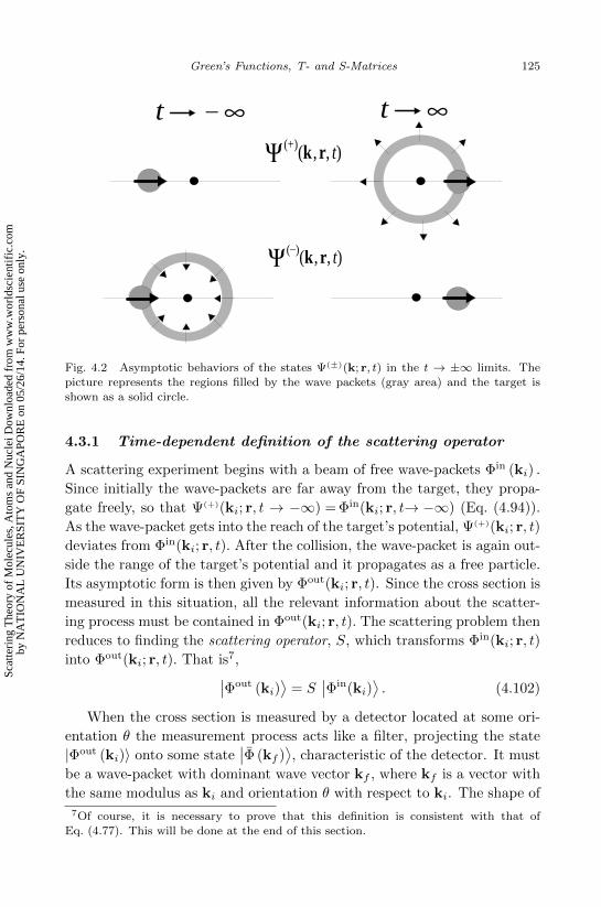
along the k-direction and an incoming spherical wave-packet. To summa-

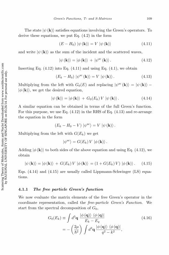
rize the above discussion, we present in figure 4.2 a schematic representation

of the asymptotic behaviors of the wave-packets Ψ(±)(k; r, t).

The states Ψ(±)(k; r, t) can be obtained from the plane-wave-packet

Φ(k; r, t) through the action of the operators Ω(±). To prove this point,

we replace ψ(±) (k) → Ω(±)φ (k) in Eqs. (4.89) and (4.96), and move Ω(±)

out of the integral. We get

|Ψ(±)(k; t)〉 = Ω(±) |Φ(k; t)〉 . (4.100)

Combining Eq. (4.100) with the asymptotic limits of Eqs. (4.93) and (4.99),

we obtain

Ω(±) = limt′→±∞

[e−iH (t′−t)/~ eiH0 (t′−t)/~

]. (4.101)

Acting on the free wave-packet at any time t, the operator Ω(+) propagates

it as a free particle backwards in time to t′ → −∞, where the free wave-

packet coincides with Ψ(+)(k; r, t′), and then brings it back to the time t

with the full propagator. The operator Ω(−) carries out the free evolution to

the distant future, where the free wave-packet coincides with Ψ(−)(k; r, t′),

and then brings it back to t with the full propagator.

Sca

tteri

ng T

heor

y of

Mol

ecul

es, A

tom

s an

d N

ucle

i Dow

nloa

ded

from

ww

w.w

orld

scie

ntif

ic.c

omby

NA

TIO

NA

L U

NIV

ER

SIT

Y O

F SI

NG

APO

RE

on

05/2

6/14

. For

per

sona

l use

onl

y.



t _ ∞ t ∞

Ψ

(+)(k , r, t)

Ψ

(_)(k , r, t)

Fig. 4.2 Asymptotic behaviors of the states Ψ(±)(k; r, t) in the t → ±∞ limits. Thepicture represents the regions filled by the wave packets (gray area) and the target is

shown as a solid circle.

4.3.1 Time-dependent definition of the scattering operator

A scattering experiment begins with a beam of free wave-packets Φin (ki) .

Since initially the wave-packets are far away from the target, they propa-

gate freely, so that Ψ(+)(ki; r, t → −∞) = Φin(ki; r, t→ −∞) (Eq. (4.94)).

As the wave-packet gets into the reach of the target’s potential, Ψ(+)(ki; r, t)

deviates from Φin(ki; r, t). After the collision, the wave-packet is again out-

side the range of the target’s potential and it propagates as a free particle.

Its asymptotic form is then given by Φout(ki; r, t). Since the cross section is

measured in this situation, all the relevant information about the scatter-

ing process must be contained in Φout(ki; r, t). The scattering problem then

reduces to finding the scattering operator, S, which transforms Φin(ki; r, t)

into Φout(ki; r, t). That is7,∣∣Φout (ki)⟩

= S∣∣Φin(ki)

⟩. (4.102)

When the cross section is measured by a detector located at some ori-

entation θ the measurement process acts like a filter, projecting the state

|Φout (ki)〉 onto some state∣∣Φ (kf )

⟩, characteristic of the detector. It must

be a wave-packet with dominant wave vector kf , where kf is a vector with

the same modulus as ki and orientation θ with respect to ki. The shape of

7Of course, it is necessary to prove that this definition is consistent with that of

Eq. (4.77). This will be done at the end of this section.

Sca

tteri

ng T

heor

y of

Mol

ecul

es, A

tom

s an

d N

ucle

i Dow

nloa

ded

from

ww

w.w

orld

scie

ntif

ic.c

omby

NA

TIO

NA

L U

NIV

ER

SIT

Y O

F SI

NG

APO

RE

on

05/2

6/14

. For

per

sona

l use

onl

y.



the packet depends on the energy resolution and detector opening. How-

ever, we have shown in chapter 1 that under typical conditions the cross sec-

tion is independent of the detailed shape of the wave-packet. In this way, we

can adopt the shape of the incident packet and replace∣∣Φ (kf )

⟩' |Φ (kf )〉 .

Therefore, the relevant information for the elastic scattering cross section

are contained in the S-matrix elements,

Sfi ≡ 〈Φ (kf )| S |Φ(ki)〉 = 〈Φ (kf )∣∣Φout(ki)

⟩. (4.103)

Above, we use the simplified notation: |Φout(ki)〉 = S∣∣Φin(ki)

⟩→

S |Φ(ki)〉 .

In Eq. (4.103), |Φ (kf )〉 and |Φout(ki)〉 are asymptotic forms of exact

states when the measurement takes place, i.e. t→ +∞. However, since H

is hermitian, the scalar product between these states - and hence Sfi - is

conserved along the collision. Therefore, the S-matrix will have the same

value if evaluated at an arbitrary time t0. For this purpose, it is necessary

to use the full propagator to take the asymptotic states from t = ∞ to

t = t0. According to Eqs. (4.95) and (4.99), this propagation yields∣∣Φout(ki)⟩→ |Ψ(+) (ki)〉 and |Φ (kf )〉 → |Ψ(−) (kf )〉 .

Eq. (4.103) then becomes

Sfi = 〈Ψ(−) (kf ) |Ψ(+) (ki) 〉 (4.104)

or, using Eq. (4.100),

Sfi = 〈Φ (kf )|Ω(−)†Ω(+) |Φ (ki)〉 . (4.105)

Since Eq. (4.105) holds for any pair of states, we can write

S = Ω(−)†Ω(+) ,

as given by Eq. (4.77).

The time-dependent and time-independent approaches to the S-matrix

are equivalent. Even if one uses the time-dependent definition of the Møller

operators (Eq. (4.101)) in Eq. (4.77), the S-matrix turns out to be time-

independent. One gets

S = limt1→−∞t2→ ∞

[eiH0t2/~ e−iH(t2−t1)/~ e−iH0t1/~

]. (4.106)

Sca

tteri

ng T

heor

y of

Mol

ecul

es, A

tom

s an

d N

ucle

i Dow

nloa

ded

from

ww

w.w

orld

scie

ntif

ic.c

omby

NA

TIO

NA

L U

NIV

ER

SIT

Y O

F SI

NG

APO

RE

on

05/2

6/14

. For

per

sona

l use

onl

y.



4.3.2 Energy conservation

We now prove the important property:

[H0, S] = 0 . (4.107)

This equation implies that the energy is conserved in the scattering process.

The starting point is the so-called interwining relation

HΩ(±) = Ω(±)H0. (4.108)

To prove this relation, we write Ω(±) as in Eq. (4.101) and calculate the

quantity

eiHtΩ(±) = eiHt limt′→±∞

[e−

i~H t′ e

i~H0 t

′]

(4.109)

= limt′→±∞

[e−

i~H (t′−t) e

i~H0 t

′].

Calling τ = t′ − t, we can write

eiHtΩ(±) = limτ→±∞

[e−

i~H τ e

i~H0τ

]ei~H0 t ,


eiHtΩ(±) = Ω(±)ei~H0 t .

Taking derivative of both sides with respect to t and setting t = 0, we have

the proof of Eq. (4.108).

Let us now evaluate the commutator [H0, S] . Using Eq. (4.77), we can

write

[H0, S] = H0S − Ω(−)†Ω(+)H0.

Applying the interwining relation, we can replace Ω(+)H0 = HΩ(+) and the

above equation takes the form

[H0, S] = H0S − Ω(−)†H Ω(+) . (4.110)

Since H† = H and H†0 = H0, we can write Ω(−)†H = (HΩ(−))†

or, using

again the interwining relation,

Ω(−)†H = (HΩ(−))†

= (Ω(−)H0)†

= H0Ω(−)† .

Inserting this result into Eq. (4.110), we obtain

[H0, S] = H0S −H0Ω(−)†Ω(+) = H0S −H0S = 0 .

Sca

tteri

ng T

heor

y of

Mol

ecul

es, A

tom

s an

d N

ucle

i Dow

nloa

ded

from

ww

w.w

orld

scie

ntif

ic.c

omby

NA

TIO

NA

L U

NIV

ER

SIT

Y O

F SI

NG

APO

RE

on

05/2

6/14

. For

per

sona

l use

onl

y.



4.3.3 Time-reversal

Although in actual physical system time develops towards increasing val-

ues, it is interesting to discuss states for which time flows backwards (see

e.g. [Messiah (1999)]). Let us first consider classical solutions of the equa-

tions of motion for a standard Lagrangian, which depends on velocities

quadratically. In this case, the Lagrangian has the time-reversal symmetry,

so that for each solution r(t); r(t), there exists a time reversed solution

rT(t); rT(t). These solutions are connected by the relations

rT(t) = r(−t) and rT(t) = −r(−t) . (4.111)

Similar properties are found in Quantum Mechanics with hermitian

Hamiltonian, which have time-reversal symmetry. Let us consider the

Schrodinger equation

Hψ(r, t) = i~∂ψ(r, t)

∂t.

We now take its hermitian conjugate and make the replacement t → −t.For hermitian Hamiltonians, we recover the original equation. Therefore,

this procedure gives rise to the new solution

ψT(r, t) = ψ∗(r,−t) . (4.112)

The transformation ψ → ψT is performed by the time-reversal operator8,

Tψ(r, t) = ψT(r, t) = ψ∗(r,−t). (4.113)

The operator T is fully determined (except for a meaningless global phase)

by its effects on the position and momentum operators,

TrT† = r and TpT† = −p . (4.114)

Furthermore, since this operator expresses a symmetry of the Hamiltonian,

it must be unitary or anti-unitary. Therefore, we can write

THT† = H and TT† = T†T =1. (4.115)

Applying the time reversal transformation on the commutator [ri, pi] = i~and using Eqs. (4.114) and (4.115) we get

T [ri, pi]T† = T (i~)T† = −i~ , (4.116)

which indicates that T is an anti-unitary operator.8This operator is discussed in standard Quantum Mechanics text books like [Messiah

(1999)]. A nice discussion of this operator aiming at scattering theory can be found in

[Taylor (2006)].

Sca

tteri

ng T

heor

y of

Mol

ecul

es, A

tom

s an

d N

ucle

i Dow

nloa

ded

from

ww

w.w

orld

scie

ntif

ic.c

omby

NA

TIO

NA

L U

NIV

ER

SIT

Y O

F SI

NG

APO

RE

on

05/2

6/14

. For

per

sona

l use

onl

y.



An important consequence of the above discussion is the time-reversal

transformation of the time-development operators

T[e−iHt/~

]T† = eiHt/~ (4.117)

T[e−iH0 t/~

]T† = eiH0 t/~ . (4.118)

For stationary scattering states, Eq. (4.112) becomes

[ψ(r)]T = ψ∗(r) . (4.119)

In particular, the time-reversal conjugate of φ(k; r) is

[φ(k; r)]T =

(1

(2π)3/2

eik·r

)∗= φ(−k; r) . (4.120)

We now consider the time-reversal transformation on the Møller oper-

ators and the scattering states. Using the representation of Eq. (4.101),

the invariance of H and H0, and the transformation law of the time-

development operators associated with H and H0 (Eqs. (4.117) and

(4.118)), we get

TΩ(±)T† = Ω(∓). (4.121)

The time-reversal conjugates of the scattering states are obtained from

Eq. (4.52) with the help of the above equations

|ψ(±) (k)〉T = T |ψ(±) (k)〉 = TΩ(±) |φ (k)〉

= TΩ(±)T†T |φ (k)〉 = Ω(∓) |φ (−k)〉 =∣∣∣ψ(∓) (−k)

⟩. (4.122)

Therefore, we can write

[ψ(±)(k; r)]∗

= ψ(∓)(−k; r). (4.123)

Eq. (4.123) can be used to derive the asymptotic form of ψ(−)(k; r). Since

ψ(−)(k; r) = [ψ(+)(−k; r)]∗, (4.124)

Eq. (2.3) yields

ψ(−)(k; r)→ A

[eik·r + f∗(π − θ) e

−ikr

r

]. (4.125)

Note that the transformation k→ −k leads to the changes θ → π − θ in

the argument of the above scattering amplitude.

Using Eq. (4.122), in Eq. (4.79), we obtain the S-matrix in terms of

outgoing waves and their time-reversal conjugates

Sk′,k =⟨

[ψ(+) (−k′)]T

∣∣∣ψ(+) (k)⟩. (4.126)

Sca

tteri

ng T

heor

y of

Mol

ecul

es, A

tom

s an

d N

ucle

i Dow

nloa

ded

from

ww

w.w

orld

scie

ntif

ic.c

omby

NA

TIO

NA

L U

NIV

ER

SIT

Y O

F SI

NG

APO

RE

on

05/2

6/14

. For

per

sona

l use

onl

y.



4.4 Scattering from non-local separable potentials

In this section we discuss an exactly soluble problem: scattering from sep-

arable potentials.

When one evaluates matrix-elements in the coordinate representation,

the operators in Quantum Mechanics fall into two categories: local and

non-local. Local operators are those whose matrix-elements have the form

U(r, r′) ≡ 〈r|U |r′〉 = U(r) δ(r− r′). (4.127)

Non-local operators are those which do not have this property. Most of the

operators appearing in simple problems in quantum mechanics are local.

In this category are the momentum and kinetic energy operators and the

majority of the potentials describing interactions of physical systems.

However, there are situations where non-local potentials emerge natu-

rally. One example is the Hartree-Fock approximation for systems of many

interacting identical fermions. In this case, the single particle orbitals sat-

isfy a Schrodinger equation where the potential is the sum of a local term

and a non-local term. The latter arises from the exchange of identical parti-

cles. Another example is the potential describing the scattering of clusters

of identical particles (see chapter 6). In this case, the wave function for the

relative projectile-target motion satisfies also an equation with a non-local

potential, arising from exchange. This can be seen explicitly in approximate

treatments of the scattering problem, like the Resonating Group Method

(for a detailed description of this method see, e.g., [Friedrich (1981)]).

In general, the matrix-elements of the potential can be written

V (r, r′) = V L(r) δ(r− r′) + V NL(r, r′), (4.128)

where V L and V NL stand respectively for the local and non-local parts of

the potential. Accordingly, the stationary Schrodinger’s equation takes the

more complicated integro-differencial form[− ~2

2µ∇2

r + V L(r)

]ψ(r) +

∫d3r′ V NL(r, r′)ψ(r′) = E ψ(r) . (4.129)

Although this equation looks more complicated than those for local

potentials, the Scattering problem can be easily solved in the case of a

strictly non-local hermitian potential (V L(r) = 0) that can be approximated

by the separable form

V (r, r′) = v(r) v(r′), (4.130)

Sca

tteri

ng T

heor

y of

Mol

ecul

es, A

tom

s an

d N

ucle

i Dow

nloa

ded

from

ww

w.w

orld

scie

ntif

ic.c

omby

NA

TIO

NA

L U

NIV

ER

SIT

Y O

F SI

NG

APO

RE

on

05/2

6/14

. For

per

sona

l use

onl

y.



with v representing a real function of the position vector. Using Dirac’s

notation for the operator V ,

V = |v〉〈v|, (4.131)

and using Eq. (4.45), one gets the scattering amplitude

f(θ) = −2π2

(2µ

~2

) ⟨φ (k′)

∣∣∣v⟩ ⟨v|ψ(+) (k)⟩. (4.132)

The first scalar product at the RHS of Eq. (4.132),

〈φ (k′) |v〉 =1

(2π)3/2

∫d3r e−ik

′·r v(r) , (4.133)

is simply the Fourier transform of the function v(r). To obtain the

scalar product 〈v|ψ(+) (k)〉, we write the Lippmann-Schwinger equation for

|ψ(+) (k)〉 (Eq. (4.38)),

|ψ(+) (k)〉 = |φ (k) 〉 + G(+)

0 (E)|v〉〈v|ψ(+) (k)〉 , (4.134)

and take scalar product of both sides with 〈v| . Eq. (4.134) becomes

〈v|ψ(+) (k)〉 = 〈v|φ (k)〉 + 〈 v|G(+)

0 (E)|v〉〈v|ψ(+) (k)〉.

Solving this equation for 〈v|ψ(+) (k)〉 one obtains

〈v|ψ(+) (k)〉 =〈v|φ (k)〉

1− 〈 v|G(+)

0 (E) |v〉. (4.135)

The expectation value 〈 v|G(+)

0 (E) |v〉 appearing in the above equation can

easily be calculated. Using the explicit form of the free particle’s Green’s

function (Eq. (4.37)), one gets

〈 v|G(+)

0 (E) |v〉 = − µ

2π~2

∫ ∫d3r d3r′ v∗(r)

e ik |r−r′|

|r− r′|v(r′).

To evaluate the scattering amplitude, we Insert Eq. (4.135) into

Eq. (4.132). One then obtains the closed expression,

f(θ) = −2π2

(2µ

~2

)〈φ (k′) |v〉〈v|φ (k)〉1− 〈 v| G(+)

0 (E) |v〉, (4.136)

and the cross section is given by the usual expression

dσel(θ)

dΩ= |f(θ)|2 .

Sca

tteri

ng T

heor

y of

Mol

ecul

es, A

tom

s an

d N

ucle

i Dow

nloa

ded

from

ww

w.w

orld

scie

ntif

ic.c

omby

NA

TIO

NA

L U

NIV

ER

SIT

Y O

F SI

NG

APO

RE

on

05/2

6/14

. For

per

sona

l use

onl

y.



It is straightforward to generalize the above procedure for non-local

potentials that can be represented by a sum of n separable terms, namely,

V =n∑λ=1

|vλ〉〈vλ| . (4.137)

In this case, the scattering amplitude is

f(θ) = −2π2

(2µ

~2

) n∑λ=1

〈φ (k′) |vλ〉〈vλ|ψ(+) (k)〉. (4.138)

The scalar products 〈φ (k′) |vλ〉 are trivial Fourier transforms of the func-

tions vλ(r), as in Eq. (4.133), and the factors 〈vλ|ψ(+) (k)〉 can be obtained

similarly to the previous case of separable potentials with a single term.

One takes scalar products of the Lippmann-Schwinger equation by each of

the factors 〈vλ|. One gets the equations

〈vλ|ψ(+) (k)〉 = 〈vλ|φ (k)〉

+n∑

λ′=1

〈 vλ|G(+)(E)|vλ′〉〈vλ′ |ψ(+) (k)〉 , λ = 1, ..., n .

This corresponds to a system of coupled linear equations with the general

form

A11X1 +A12X2 + ......+A1nXn = Y1

A21X1 +A22X2 + ......+A2nXn = Y2

............................................................

An1X1 +An2X2 + ......+AnnXn = Yn, (4.139)

where

Xλ = 〈vλ|ψ(+) (k)〉 ,Aλλ′ = δλλ′ − 〈 vλ|G(+)(E)|vλ′〉 ,Yλ = 〈vλ|φ (k)〉 .

This system can be easily be solved by standard methods. Using the so-

lutions 〈vλ|ψ(+)

k 〉 = Xλ in Eq. (4.138) we get the scattering amplitude and

then the cross-section.

Scattering from non-local separable potentials are encountered in sev-

eral situations. One example in many-body scattering can be found in

section 10.2.2.

Sca

tteri

ng T

heor

y of

Mol

ecul

es, A

tom

s an

d N

ucle

i Dow

nloa

ded

from

ww

w.w

orld

scie

ntif

ic.c

omby

NA

TIO

NA

L U

NIV

ER

SIT

Y O

F SI

NG

APO

RE

on

05/2

6/14

. For

per

sona

l use

onl

y.



4.5 Scattering from the sum of two potentials

In section 4.1 we wrote the Hamiltonian as H = H0 + V, with H0 being

the kinetic energy operator, K, and V the total potential. We then showed

that the exact solutions |ψ(±) (k)〉 and the plane waves |φ (k)〉 are related

by Lippmann-Schwinger equations. In some situations, it is convenient to

split the total potential into two parts,

V = V1 + V2, (4.140)

and derive Lippmann-Schwinger equations involving the states distorted

by the potential V1 alone, which will be denoted by |χ(±) (k)〉 . They are

scattering states when one sets V2 = 0. Thus, they satisfy the Schrodinger

equation

(E −H1) |χ(±) (k)〉 = 0 , (4.141)

with

H1 = K + V1. (4.142)

In the r →∞ limit, the distorted states have the asymptotic forms

χ(+)(k; r)→ A

(eik·r + f1(θ)

eikr

r

), (4.143)

χ(−)(k; r)→ A

(eik·r + f∗1 (π − θ) e

−ikr

r

). (4.144)

Above, f1(θ) is the scattering amplitude associated with the potential V1.

The distorted states satisfy the Lippmann-Schwinger equations

|χ(±) (k)〉 = |φ (k)〉+G(±)

0 (Ek) V1 |χ(±) (k)〉 (4.145)

and

|χ(±) (k)〉 =[1 +G(±)

1 (Ek) V1

]|φ (k)〉 , (4.146)

where

G(±)

1 (E) =1

E −H1 ± iε, (4.147)

and they obey the completeness relation∫|χ(±) (q)〉 d3q 〈χ(±) (q)| +

∑n

|χn〉〈χn| = 1. (4.148)

Sca

tteri

ng T

heor

y of

Mol

ecul

es, A

tom

s an

d N

ucle

i Dow

nloa

ded

from

ww

w.w

orld

scie

ntif

ic.c

omby

NA

TIO

NA

L U

NIV

ER

SIT

Y O

F SI

NG

APO

RE

on

05/2

6/14

. For

per

sona

l use

onl

y.



Above, |χn〉 stands for the bound states that the potential V1 may possibly

have.

Applying the procedures of section 4.1 to the Schrodinger equation with

the full potential,

(E −H) |ψ(±) (k)〉 ≡ (E −H1 − V2)∣∣∣ψ(±) (k)

⟩= 0,

one easily obtains the Lippmann-Schwinger equations for |ψ(±) (k)〉 (see

problem 2),

|ψ(±) (k)〉 = |χ(±) (k)〉+G(±)

1 (Ek) V2 |ψ(±) (k)〉 (4.149)

and

|ψ(±) (k)〉 = [1 +G(±) (Ek) V2] |χ(±) (k)〉 . (4.150)

4.5.1 The Gell-Mann Goldberger relations

It is useful to introduce the T-matrix associated with the potential V1 alone

(setting V2 = 0). It is given by Eq. (4.63), which in this case becomes

T (1)

k′,k =⟨φ (k′)

∣∣V1

∣∣χ(+) (k)⟩. (4.151)

This matrix is related to the T-matrix for the total potential, Tk′,k, through

the Gell-Mann Goldberger relation, also called the two-potential formula,

Tk′,k = T (1)

k′,k + 〈χ(−) (k′)|V2 |ψ(+) (k)〉 . (4.152)

This expression will be proved below.

As a first step, we rewrite the Lippmann-Schwinger equations involving

|φ (k)〉 and |ψ(+) (k)〉,

|ψ(+) (k)〉 = |φ (k)〉+G(+)

0 (Ek) [V1 + V2] |ψ(+) (k)〉 (4.153)

and

|ψ(+) (k)〉 = 1 +G(+)(Ek) [V1 + V2] |φ (k)〉 . (4.154)

Using the property9 G(−)†0 = G(+)

0 , the hermitian conjugate of Eq. (4.145)

can be written

〈φ (k′)| = 〈χ(−) (k′)| − 〈χ(−) (k′)|V1G(+)

0 . (4.155)

Inserting Eq. (4.155) into the definition of the T-matrix ,

Tk′,k ≡⟨φ (k′)

∣∣∣ (V1 + V2)∣∣∣ψ(+) (k)

⟩, (4.156)

9Since in this proof we are dealing with matrix-elements on-the-energy-shell, Ek = Ek′ ,

the energy labels become superfluous.

Sca

tteri

ng T

heor

y of

Mol

ecul

es, A

tom

s an

d N

ucle

i Dow

nloa

ded

from

ww

w.w

orld

scie

ntif

ic.c

omby

NA

TIO

NA

L U

NIV

ER

SIT

Y O

F SI

NG

APO

RE

on

05/2

6/14

. For

per

sona

l use

onl

y.



we get

Tk′,k = 〈χ(−) (k′)| (V1 + V2) |ψ(+) (k)〉

− 〈χ(−) (k′)|V1

G(+)

0

(V1 + V2

) ∣∣∣ψ(+) (k)⟩. (4.157)

Now, we use Eq. (4.153) to write

G(+)

0 [V1 + V2] |ψ(+) (k)〉 = |ψ(+) (k)〉 −∣∣∣φ (k)

⟩, (4.158)

and replace the term within curly brackets in Eq. (4.157) by the above

result. We obtain

Tk′,k = 〈χ(−) (k′) |V1 + V2 |ψ(+) (k)〉− 〈χ(−) (k′) |V1 |ψ(+) (k)〉+ 〈χ(−) (k′) |V1 |φ (k)〉 ,

or

Tk′,k =⟨χ(−) (k′)

∣∣∣V1

∣∣∣φ (k)⟩

+⟨χ(−) (k′)

∣∣∣V2

∣∣∣ψ(+) (k)⟩. (4.159)

Now we re-write the first term at the RHS of Eq. (4.159) in terms of the

Møller operator associated with H1 and use Eq. (4.71). Eq. (4.159) then

becomes⟨χ(−) (k′)

∣∣∣V1

∣∣∣φ (k)⟩

=⟨φ (k′)

∣∣∣Ω(−)† V1

∣∣∣φ (k)⟩

= T (1)

k′,k. (4.160)

Inserting the above result into Eq. (4.159), we get the proof of the Gell-

Mann Goldberger relation (Eq. (4.152)).

4.5.2 The Distorted Wave series

The Gell-Mann Goldberger relations can be written as power series. Ap-

plying recursively Eq. (4.149) on Eq. (4.152), we get

Tk′,k =⟨φ (k′)

∣∣∣V1

∣∣∣χ(+) (k)⟩

+⟨χ(−) (k′)

∣∣∣V2

∞∑m=0

(G(+)

1 (Ek)V2

)m ∣∣∣χ(+) (k)⟩. (4.161)

If one uses the spectral representation10 of G(+)

1 (Ek),

G(+)1 (Ek) =

∫d3q

∣∣χ(+) (q)⟩ ⟨χ(+) (q)

∣∣Ek − Eq + iε

, (4.162)

10For simplicity, we are neglecting the possibility that the potential V1 have boundstates. Bound states would lead to extra terms in the expansion, arising from the discrete

summation of Eq. (4.148).

Sca

tteri

ng T

heor

y of

Mol

ecul

es, A

tom

s an

d N

ucle

i Dow

nloa

ded

from

ww

w.w

orld

scie

ntif

ic.c

omby

NA

TIO

NA

L U

NIV

ER

SIT

Y O

F SI

NG

APO

RE

on

05/2

6/14

. For

per

sona

l use

onl

y.



Eq. (4.161) becomes

Tk′,k =⟨φ (k′)

∣∣∣V1

∣∣∣χ(+) (k)⟩

+ 〈χ(−) (k′)| V2 |χ(+) (k)〉

+

∫d3q〈χ(−) (k′)| V2 |χ(+) (q)〉〈χ(+) (q)|V2 |χ(+) (k)〉

Ek − Eq + iε

+ higher order terms. (4.163)

This is known as the Distorted Wave series. Truncating the expansion of

Eq. (4.161) after m = 0, (i.e. keeping only the first line of Eq. (4.163)), we

get the Distorted Wave Born Approximation (DWBA). This approximation

will be considered in detail in chapter 5 and in chapter 11, in the cases of

potential scattering and many-body scattering, respectively.

4.6 Partial-wave expansions

In this section we carry out partial-wave expansion of the Lippmann-

Schwinger equations. As a starting point, we introduce the orthonormal

sets of states |φ(Elm)〉 and |ψ(Elm)〉 , which are eigenstates of the op-

erators L2 and Lz, with eigenvalues ~2l(l + 1) and ~m, respectively. They

satisfy the Schrodinger equations

(E −H0) |φ(Elm)〉 = 0 (4.164)

(E −H) |ψ(Elm)〉 = 0 (4.165)

and are normalized as to satisfy the relations

〈φ (E′l′m′) |φ(Elm)〉 = δll′ δmm′ δ(E − E′) (4.166)

〈ψ (E′l′m′) |ψ (Elm)〉 = δll′ δmm′ δ(E − E′) . (4.167)

In the coordinate representation, the wave functions φ(Elm; r) and

ψ(Elm; r) are products of Spherical Harmonics Ylm(r) with appropriate

radial wave functions. The completeness relation for the states |φ(Elm)〉has the form ∑

lm

∫|φ(Elm)〉 dE 〈φ(Elm)| = 1. (4.168)

The solutions of the Schrodinger equation with the Hamiltonian H,

ψ(Elm; r), depend on the particular potential of the problem while the

free spherical waves φ(Elm; r) are completely determined (see chapter 2),

except for an arbitrary global phase. They can be written as

φ(Elm; r) = All(kr)

krYlm(r), (4.169)

Sca

tteri

ng T

heor

y of

Mol

ecul

es, A

tom

s an

d N

ucle

i Dow

nloa

ded

from

ww

w.w

orld

scie

ntif

ic.c

omby

NA

TIO

NA

L U

NIV

ER

SIT

Y O

F SI

NG

APO

RE

on

05/2

6/14

. For

per

sona

l use

onl

y.



where k =√

2µE/~ and Al is a normalization constant. Using the orthonor-

mality of the Spherical Harmonics and the radial integral of Ricatti-Bessel

functions (Eq. (2.26)), Eq. (4.166) yields

|Al |2 =2µk

π~2→ Al = il

(2µk

π~2

)1/2

, (4.170)

where the arbitrary phase of Al was chosen to be il. We can use an analo-

gous procedure for the wave functions ψ(Elm; r). We write

ψ(Elm; r) = il(

2µk

π~2

)1/2ul(k, r)

krYlm(r) (4.171)

= il(

2µk

π~2

)1/2ul(k, r)

krYlm(r) eiδl , (4.172)

were ul(k, r) and ul(k, r) are solutions of the radial equation with different

choices of phase, as discussed in chapter 2. As will become clear, the inclu-

sion of the arbitrary phase eiδl leads to simpler expressions. Eq. (4.167)

requires that the radial wave functions be normalized as,∫ ∞0

u∗l (k, r)ul(k′, r) dr =

π

2δ(k − k′) . (4.173)

Frequently, it is convenient to expand the plane waves and the scatter-

ing states in terms of the corresponding orthonormal angular momentum

eigenstates, as

φ(k; r) =∑l′,m′

∫dE′ CE′l′m′(k) φ(E′l′m′; r), (4.174)

ψ(+)(k; r) =∑l′,m′

∫dE′ CE′l′m′(k) ψ(E′l′m′; r). (4.175)

The expansion coefficients,

CE′l′m′(k) = 〈φ(E′l′m′) |φ(k)〉 , (4.176)

can be evaluated explicitly with the help of Eqs. (2.44a), (4.169), (4.170)

and the orthogonality relations of the Ricatti-Bessel functions (Eq. (2.26)).

One gets,

CE′l′m′(k) =~√µk

Y ∗l′m′(k) δ(E − E′), (4.177)

where E = ~2k2/2µ. The plane waves and the scattering states are then

given by

φ(k; r) =~√µk

∑l,m

Y ∗lm(k) φ(Elm; r) (4.178a)

=1

(2π)3/2

∑lm

4π Y ∗lm(k) Ylm(r) iljl(kr)

kr(4.178b)

Sca

tteri

ng T

heor

y of

Mol

ecul

es, A

tom

s an

d N

ucle

i Dow

nloa

ded

from

ww

w.w

orld

scie

ntif

ic.c

omby

NA

TIO

NA

L U

NIV

ER

SIT

Y O

F SI

NG

APO

RE

on

05/2

6/14

. For

per

sona

l use

onl

y.



and

ψ(+)(k, r) =~√µk

∑l,m

Y ∗lm(k) ψ(Elm; r). (4.179)

Using the explicit form of ψ(Elm; r), Eq. (4.179) becomes (Eq. (2.57a) with

A = (2π)−3/2

)

ψ(+)(k, r) =1

(2π)3/2

∑lm

4π Y ∗lm(k) Ylm(r) ilul(k, r)

kr(4.180a)

=1

(2π)3/2

∑l

(2l + 1) Pl(cos θ) ilul(k, r)

kr. (4.180b)

The partial-wave expansion for ψ(−)(k, r) is easily obtained from the

above equations, through the relation ψ(−)(k, r) = (ψ(+)(−k, r))∗

(see sec-

tion 4.3.3). Considering the property Ylm(−k) = (−)l Ylm(k), we get11

ψ(−)(k, r) =1

(2π)3/2

∑lm

4π Y ∗lm(k) Ylm(r) ilu∗l (k, r)

kr(4.181a)

=1

(2π)3/2

∑l

(2l + 1) Pl(cos θ) ilu∗l (k, r)

kr. (4.181b)

To derive the partial-wave projected Lippmann-Schwinger equation, we

carry out the partial-wave expansion of G(±)

0 (E; r, r′) as12

G(±)

0 (E; r, r′) =1

rr′

∑lm

Y ∗lm(r) g(±)

0,l (r, r′) Ylm(r′). (4.182)

Since we are supposing that the potential is spherically symmetric, the

Hamiltonian is rotationally invariant. Therefore, the Green’s function is

diagonal in the angular momentum representation. We then insert this ex-

pansion and the expansions for the wave functions (Eqs. (2.44a) and (2.57a)

with A = 1/(2π)3/2) into the Lippmann-Schwinger equation (Eq. (4.40)).

Using the linear independence and the orthonormality of the spherical har-

monics, we get

ul(k, r) = l(kr) +

∫dr′ g(+)

0,l (r, r′)V (r′) ul(k, r′). (4.183)

In terms of radial functions with the phase chosen as in Eq. (2.41a), the

above equation becomes

eiδl ul(k, r) = l(kr) +

∫dr′ g(+)

0,l (r, r′)V (r′) eiδl ul(k, r′). (4.184)

11We recall that u∗l (k, r) = e−iδl ul(k, r), where ul(k, r) is the real radial wave function,which has the asymptotic behavior ul(k, r)→ sin(kr − lπ/2 + δl) (see chapter 2).12The use of the factor 1/rr′ in the partial-wave expansion of the Green’s functions leads

to a simpler form of the Lippmann-Schwinger equations for u(±)

l (k, r).

Sca

tteri

ng T

heor

y of

Mol

ecul

es, A

tom

s an

d N

ucle

i Dow

nloa

ded

from

ww

w.w

orld

scie

ntif

ic.c

omby

NA

TIO

NA

L U

NIV

ER

SIT

Y O

F SI

NG

APO

RE

on

05/2

6/14

. For

per

sona

l use

onl

y.



Equations involving the Green’s function g(−)

0,l could be obtained using the

partial-wave expansion of ψ(−)(k; r) (Eq. (4.181a). One gets,

u∗l (k, r) = l(kr) +

∫dr′ g(−)

0,l (r, r′)V (r′)u∗l (k, r′) (4.185)

or

e−iδl ul(k, r) = l(kr) +

∫dr′ g(−)

0,l (r, r′)V (r′) e−iδl ul(k, r′). (4.186)

However, these equations are not lineraly independent of those involving

g(+)

0,l , since they are simply their complex conjugates.

Equivalent equations can be obtained with the full Green’s function.

Making the expansion

G(±)(E; r, r′) =1

rr′

∑lm

Y ∗lm(r) g(±)

l (r, r′) Ylm(r′) (4.187)

and following the same procedures, we obtain

ul(k, r) = l(kr) +

∫dr′ g(+)

l (r, r′)V (r′) l(kr′). (4.188)

and

eiδl ul(k, r) = l(kr) +

∫dr′ g(+)

l (r, r′)V (r′) l(kr′). (4.189)

Similar equations can be obtained in terms of g(−)

l .

4.6.1 Partial-wave projection of the S- and the T-matrices

It is also convenient to carry out the partial-wave expansion of the T-matrix

between states on the same energy-shell. For this purpose, we start from

its definition (Eq. (4.63)) and use the partial-wave expansions of ψ(+) (k)

(Eq. (4.179)) and φ (k′) (Eq. (4.178a). With the help of Eqs. (4.169) and

(4.171), we get

Tk′,k ≡⟨φ (k′)

∣∣∣V ∣∣∣ψ(+) (k)⟩

=~2

µk

∑lm

Ylm(k′)Y ∗lm(k)Tl(Ek), (4.190)

where we have introduced the partial-wave component of the T-matrix be-

tween states on the same energy-shell,

Tl(Ek) = 〈φ(Elm)|V |ψ (Elm)〉 (4.191a)

=k

πEk

∫ ∞0

dr l(kr)V (r)ul(k, r) (4.191b)

=k

πEkeiδl

∫ ∞0

dr l(kr)V (r) ul(k, r) . (4.191c)

Sca

tteri

ng T

heor

y of

Mol

ecul

es, A

tom

s an

d N

ucle

i Dow

nloa

ded

from

ww

w.w

orld

scie

ntif

ic.c

omby

NA

TIO

NA

L U

NIV

ER

SIT

Y O

F SI

NG

APO

RE

on

05/2

6/14

. For

per

sona

l use

onl

y.



Using the addition theorem for the Spherical Harmonics,∑m

Ylm(k′)Y ∗lm(k) =2l + 1

4πPl(cos θ),

Eq. (4.190) becomes

Tk′,k =∑l

(2l + 1)Pl(cos θ)

[~2

4πµkTl(Ek)

]. (4.192)

A similar procedure can be followed in the case of the S-matrix. First,

we write the scattering operator in the representation of the |φ(Elm)〉 states

and use the completeness relation of Eq. (4.168). We get

Sk′,k =∑

l1m1,l2m2

∫ ∫dE1 dE2 〈φ (k′) |φ (E1l1m1)〉

× 〈φ (E1l1m1) |S |φ(E2l2m2)〉〈φ(E2l2m2)|φ (k)〉 . (4.193)

Since we are dealing with spherically symmetric potentials, the Hamiltoni-

ans H0 and H are rotationally invariant. This implies that the S-operator

is diagonal in the angular momentum representation. This becomes clear

when one writes S = Ω(−)† Ω(+), with Ω(±) given by Eq. (4.101), and re-

alizes that S commutes with any component of the angular momentum

operator. Furthermore, 〈φ (E1l1m1)| S |φ(E2l2m2)〉 must be independent

of m-values, since S also commutes with the operators J± = Jx±iJy, which

change m → m ± 1. Considering that the S-operator also commutes with

the Hamiltonian H0 (see Eq. (4.107)), we can write

〈φ (E1l1m1)| S |φ(E2l2m2)〉 = Sl1(E1) δl1l2 δm1m2δ(E1 − E2) . (4.194)

Now we use Eqs. (4.176) and (4.177) to evaluate 〈φ(k′)|φ (E1l1m1)〉 and

〈φ(E2l2m2)|φ (k)〉. Inserting the results into Eq. (4.193), we obtain

Sk′,k = δ(Ek′ − Ek)~2

µk

∑lm

Ylm(k′) Y ∗lm(k) Sl(Ek) (4.195)

= δ(Ek′ − Ek)~2

4πµk

∑l

(2l + 1)Pl(cos θ) Sl(Ek). (4.196)

Above, we have adopted the notation: l1 = l2 = l,m1 = m2 = m, Eq =

~2q2/2µ and Ek = ~2k2/2µ. Eq. (4.196) was obtained from to Eq. (4.195)

through the Addition Theorem.

Now we can relate the partial-wave components of the T- and the S-

operators. For this purpose we use in Eq. (4.82) the partial-wave expansion

Sca

tteri

ng T

heor

y of

Mol

ecul

es, A

tom

s an

d N

ucle

i Dow

nloa

ded

from

ww

w.w

orld

scie

ntif

ic.c

omby

NA

TIO

NA

L U

NIV

ER

SIT

Y O

F SI

NG

APO

RE

on

05/2

6/14

. For

per

sona

l use

onl

y.



for the T-matrix (Eq. (4.192)). We obtain,

Sk′,k = δ(k′ − k)− 2πi δ(Ek′ − Ek)∑l

(2l + 1)Pl(cos θ)

[~2

4πµkTl(Ek)

].

(4.197)

The next step is to express δ(k′−k) in terms of Ek,Ωk, Ek′ ,Ωk′ . We start

from the relation∫dΩk dk k

2 δ(k′ − k) =

∫dΩk dEk δ(Ek′ − Ek) δ(Ωk′ − Ωk). (4.198)

Writing

dEk =~2

µk

(k2 dk

),

we get

δ(k′ − k) =~2

µkδ(Ek′ − Ek) δ(Ωk′ − Ωk). (4.199)

We now use the completeness of the Spherical Harmonics to write

δ(Ωk′ − Ωk) =∑lm

Y ∗lm(Ωk′)Ylm(Ωk) =1

4π

∑l

(2l + 1)Pl(cos θ). (4.200)

Using this relation in Eq. (4.199) and inserting the result into Eq. (4.197),

we obtain

Sk′,k = δ(Ek′−Ek)∑l

(2l+1)Pl(cos θ)

[~2

4πµk(1− 2πiTl(E))

]. (4.201)

Comparing Eqs. (4.196) and Eq. (4.201), we get the desired expression

Sl(E) = 1− 2πi Tl(E). (4.202)

It is convenient to express also the scattering amplitude in terms of

Tl(E). Inserting Eq. (4.192) into Eq. (4.64), we get

f(θ) = −2π2

(2µ

~2

)~2

4πµk

∑l

(2l + 1)Pl(cos θ)Tl(E)

= −πk

∑l

(2l + 1)Pl(cos θ)Tl(E)

or

f(θ) =1

2ik

∑l

(2l + 1)Pl(cos θ) [−2πi Tl(E)] . (4.203)

Sca

tteri

ng T

heor

y of

Mol

ecul

es, A

tom

s an

d N

ucle

i Dow

nloa

ded

from

ww

w.w

orld

scie

ntif

ic.c

omby

NA

TIO

NA

L U

NIV

ER

SIT

Y O

F SI

NG

APO

RE

on

05/2

6/14

. For

per

sona

l use

onl

y.



Using Eq. (4.202), the scattering amplitude takes the form

f(θ) =1

2ik

∑l

(2l + 1)Pl(cos θ) [Sl(E)− 1] . (4.204)

This equation was derived in chapter 2 (see Eq. (2.54b)) from the asymp-

totic behavior of the wave function.

4.6.2 The partial-wave projected two-potential formula

One can also perform partial-wave expansion of the Gell-Mann Goldberger

relation. First, we write the angular momentum expansions of the distorted

waves,

χ(+)(k, r) =1

(2π)3/2

∑lm

4π Y ∗lm(k) Ylm(r) ilwl(k, r)

kr(4.205)

and

χ(−)(k, r) =1

(2π)3/2

∑lm

4π Y ∗lm(k)Ylm(r) ilw∗l (k, r)

kr. (4.206)

Next, we use the expansion of ψ(+)(k, r) (Eq. (4.180a)) and expand the

distorted and the total T-matrices as (Eq. (4.190))

Tk′,k = =~2

µk

∑lm

Ylm(k′)Y ∗lm(k) Tl(Ek)

T (1)

k′,k = =~2

µk

∑lm

Ylm(k′)Y ∗lm(k) T (1)

l (Ek), (4.207)

where

T (1)

l (Ek) =k

πEk

∫ ∞0

dr l(kr)V1(r)wl(k, r). (4.208)

Inserting these expansions into Eq. (4.152), we get the partial-wave pro-

jected Gell-Mann Goldberger relation,

Tl(Ek) = T (1)

l (Ek) +k

πEk

∫ ∞0

dr wl(k, r)V2(r)ul(k, r). (4.209)

4.7 Long range potentials

The scattering from potentials that fall off slowly13 in the r →∞ limit re-

quires special treatment. This problem was considered in chapter 3, where13Cases in which the condition limr→∞ [r V (r)] = 0 is not satisfied.

Sca

tteri

ng T

heor

y of

Mol

ecul

es, A

tom

s an

d N

ucle

i Dow

nloa

ded

from

ww

w.w

orld

scie

ntif

ic.c

omby

NA

TIO

NA

L U

NIV

ER

SIT

Y O

F SI

NG

APO

RE

on

05/2

6/14

. For

per

sona

l use

onl

y.



we discussed the scattering amplitude and the wave function in the cases

of Coulomb and Coulomb plus short range potentials. We derived an anal-

lytical expression for the Coulomb scattering amplitude (Eq. (3.29)) and

showed that the corresponding wave function is given by the partial-wave

expansion (Eq. (3.102a))

φ(+)

C (k; r) =1

(2π)3/2

∑lm

4π Y ∗lm(k) Ylm(r) il eiσlFl(η, kr)

kr. (4.210)

Above, Fl(η, kr) is the regular Coulomb wave function and σl is the

Coulomb phase shift for the lth partial-wave (see e.g. [Abramowitz and

Stegun (1972)]). Now we discuss Møller operators and the S- and the T-

matrices in Coulomb scattering.

First, we obtain the partial-wave expansion for the wave function with

incoming wave boundary condition, φ(−)C (k; r). This can be done with the

help of the time reversal property of φ(+)C (k; r). Using Eq. (4.124), we ob-

tain14

φ(−)

C (k; r) =1

(2π)3/2

∑lm

4π Y ∗lm(k) Ylm(r) il e−iσlFl(η, kr)

kr. (4.211)

This expression will be used later in this section.

Now we evaluate the on-shell matrix-elements of the transition opera-

tor15. Using Eqs. (3.29) and (4.64) we directly obtain

TC

k′,k =

(~2

2µ

)1

2π2

[η

2k sin2(θ/2)e−iη ln(sin2 θ/2) e2iσ0

]. (4.212)

It is still possible to define Møller wave operators and the S-matrix as

in the previous sections. The Møller operators are given by the condition

Ω(±)

C |φ(k)〉 = |φ(±)

C (k)〉 . (4.213)

We remark that the long range of the Coulomb field leads to serious math-

ematical problems involving the Møller operators [Dollard (1964); Alt and

14Although the partial-wave expansion for the Coulomb scattering amplitude is useless,since it does not converge, the expansions for φ

(±)C (k; r) are very Important. They are

used in the description of scattering from Coulomb plus short-range potentials.15In fact, owing to the infinite range of the Coulomb field, the transition matrix inmomentum space has no on-shell limit. However, this difficulty can be avoided evaluating

matrix-elements in the asymptotically Coulomb-modified free states [Nutt (1968); vanHaeringen (1976)]. Although we do not state it explicitly, it should be understood thatin this section the matrix-elements in the momentum representation are evaluated with

this modification.

Sca

tteri

ng T

heor

y of

Mol

ecul

es, A

tom

s an

d N

ucle

i Dow

nloa

ded

from

ww

w.w

orld

scie

ntif

ic.c

omby

NA

TIO

NA

L U

NIV

ER

SIT

Y O

F SI

NG

APO

RE

on

05/2

6/14

. For

per

sona

l use

onl

y.



Sandhas (1966)]. In the time-dependent approach, where the incident parti-

cle is represented by a wave packet, Ω(±)C is no longer given by Eq. (4.101).

In this case, the asymptotic equivalence of the Hamiltonians H and H0

breaks down, since the Coulomb field distorts the incident packet even at

asymptotic distances. However, this difficulty can be avoided with an ap-

propriate modification of Eq. (4.101) [Dollard (1964)].

The Coulomb S-matrix is given in terms of the Møller operators as

Sc = Ω(−)†

C Ω(+)

C . (4.214)

According to Eq. (4.83), the Coulomb scattering and transition operators

for a given collision energy are related by the equation

Sc(E) = 1− 2πi δ (E −H0) T c(E). (4.215)

Let us now consider the scattering from Coulomb plus short-range po-

tentials. In this case the potential is given by the sum

V (r) = VC(r) + V (r) ,

where V (r) vanishes or can be neglected for r > R. In chapter 3 we have

shown that the scattering wave function is given by the partial-wave ex-

pansion (Eq. (3.125a))

ψ(+)(k; r) =1

(2π)3/2

∑lm

4π Y ∗lm(k) Ylm(r) il eiσlul(k, r)

kr, (4.216)

where ul(k, r) is the solution of the radial equation for the lth partial-wave,

with the asymptotic form (see Eq. (3.115))

ul(k, r > R) =i

2

[H(−)

l (η, kr)− SlH(+)

l (η, kr)].

Above, H(−)

l (H(+)

l ) is the Coulomb wave function with incoming (outgoing)

wave boundary condition and Sl is the l-projected S-matrix associated with

the short-range interaction. Similarly to the case of a pure Coulomb field,

the wave function ψ(−)(k; r) can be derived from the time-reversal conjugate

of ψ(+)(−k; r) and one obtains

ψ(−)(k; r) =1

(2π)3/2

∑lm

4π Y ∗lm(k) Ylm(r) il e−iσlu∗l (k, r)

kr. (4.217)

It is convenient to write the Møller wave operators as

Ω(±) = Ω(±)

C Ω(±). (4.218)

Sca

tteri

ng T

heor

y of

Mol

ecul

es, A

tom

s an

d N

ucle

i Dow

nloa

ded

from

ww

w.w

orld

scie

ntif

ic.c

omby

NA

TIO

NA

L U

NIV

ER

SIT

Y O

F SI

NG

APO

RE

on

05/2

6/14

. For

per

sona

l use

onl

y.



In this way, Ω(±) is the operator which transforms Coulomb states∣∣φ(±)

C (k)⟩

into solutions of the Schrodinger equation with the full potential. That is

Ω(±) |φ(±)

C (k)〉 = |ψ(±)(k)〉 . (4.219)

In the time-dependent approach, these operators are given by the trivial

generalization of Eq. (4.101)

Ω(±) = limt′→±∞

e−i~H (t′−t) e

i~HC (t′−t) , (4.220)

with HC = K + VC and H = HC + V . The scattering operator associated

with the short-range interaction is defined as

S = Ω(−)† Ω(+) . (4.221)

Inserting Eq. (4.218) into Eq. (4.77), we get

S = Ω(−)†

C S Ω(+)

C (4.222)

It is useful to define a transition operator associated with the short-

range interaction as

T = V Ω(+) = Ω(−)† V . (4.223)

It is related with the full transition matrix through the Gell-Mann-

Goldberger relation. Setting in Eqs. (4.151) and (4.152)

V1 = VC, V2 = V , |χ(±) (k)〉 = |φ(±)

C (k)〉 ,

one gets

Tk′,k = 〈φ (k′)| VC |φ(+)

C (k)〉+ 〈φ(−)

C (k′)| V |ψ(+) (k)〉 (4.224)

= TC

k′,k + 〈φ(−)

C (k′)| T |φ(+)

C (k)〉 , (4.225)

or, simply

T = TC + Ω(−)†

C T Ω(+)

C . (4.226)

Inserting Eq. (4.226) into Eq. (4.83) and using Eq. (4.215), we get the

relation,

S(E) = SC(E) − 2πi δ (E −H0) Ω(−)†

C T Ω(+)

C ,

or, taking into account Eqs. (4.222) and (4.214),

Ω(−)†

C S(E) Ω(+)

C = SC(E) − 2πi δ (E −H0) Ω(−)†

C T Ω(+)

C (4.227)

= Ω(−)†

C Ω(+)

C − 2πi δ (E −H0) Ω(−)†

C T Ω(+)

C . (4.228)

Sca

tteri

ng T

heor

y of

Mol

ecul

es, A

tom

s an

d N

ucle

i Dow

nloa

ded

from

ww

w.w

orld

scie

ntif

ic.c

omby

NA

TIO

NA

L U

NIV

ER

SIT

Y O

F SI

NG

APO

RE

on

05/2

6/14

. For

per

sona

l use

onl

y.



The above equation leads to a simple relation between the partial-wave

components of S and T . First, one takes matrix-elements in the momentum

representation and let the operator δ (E −H0) act on the bra. We get⟨φ(−)

C (k′) |S |φ(+)

C (k)⟩

= 〈φ(−)

C (k′) |φ(+)

C (k)〉+ 2πi δ (E − Ek′)

⟨φ(−)

C (k′) |T |φ(+)

C (k)⟩. (4.229)

Now we carry out the partial-wave expansion of the T- and the S-

matrices in the scattering from Coulomb plus short-range potentials. For

this purpose, we follow the same procedures of section 4.6.1. In the Coulomb

case, the orthonormal states of the energy and angular momentum basis

are

φC(Elm; r) = il(

2µk

π~2

)1/2Fl(η, kr)

krYlm(r) (4.230)

and the partial-wave components of the operators S and T are defined as

Sl(E) = 〈φC(Elm)| S |φC(Elm)〉 (4.231)

and

Tl(E) = 〈φC(Elm)| T |φC(Elm)〉 = 〈φC(Elm)| V |ψ(Elm)〉 (4.232)

=k

πE

∫dr Fl(η, kr) V (r)ul(k, r), (4.233)

respectively. Proceeding as in section 4.6.1, with the replacement of

Eq. (4.177) by its Coulomb analog,

〈φC(Elm) |φ(±)

C (k)〉 =~√µkY ∗lm(k) e±iσl δ(E − Ek), (4.234)

we obtain

Sl(E) = 1− 2πi Tl. (4.235)

4.8 Evaluation of partial-wave Green’s functions

In this section we discuss the calculation of partial-wave projected Green’s

function. We begin with the case of a free particle, where the Green’s func-

tions can be determined in terms of Riccati-Bessel functions of different

kinds. We then derive an expression for the Green’s functions for an arbi-

trary potential. This expression involves the regular solution of the equa-

tion for the same potential and the solution with outgoing wave boundary

condition.

Sca

tteri

ng T

heor

y of

Mol

ecul

es, A

tom

s an

d N

ucle

i Dow

nloa

ded

from

ww

w.w

orld

scie

ntif

ic.c

omby

NA

TIO

NA

L U

NIV

ER

SIT

Y O

F SI

NG

APO

RE

on

05/2

6/14

. For

per

sona

l use

onl

y.



4.8.1 Free particle’s Green’s function

Let us now evaluate the partial-wave projected Green’s function for a

free particle, g(+)

l (E; r, r′). We start from the spectral representation of

G(+)

0 (E; r, r′) in the spherical basis16,

G(+)

0 (E; r, r′) =∑lm

∫ ∞0

dE′φ∗E′lm(r)φE′lm(r′)

E − E′ + iε

=1

rr′

∑lm

Y ∗lm(r)Ylm(r′)

[2µ

π~2

∫ ∞0

dE′

k′l(k

′r) l(k′r′)

E − E′ + iε

].

Comparing the above equation with Eq. (4.182) we get

g(+)

0,l (E; r, r′) =2µ

π~2

∫ ∞0

dE′

k′l(k

′r) l(k′r′)

E − E′ + iε. (4.236)

Changing variable: E′ → k′, we replace E′ = ~2k′2/2µ and dE′ =(~2k′/µ

)dk′ and Eq. (4.236) becomes

g(+)

0,l (E; r, r′) =2

π

(2µ

~2

)∫ ∞0

dk′l(k

′r) l(k′r′)

k2 − k′2 + iε′. (4.237)

Considering the properties of Bessel functions (see, for example, appendix

C of [Joachain (1983)]),

jl(−z) = (−)l jl(z)→ l(−z) = (−)l+1 l(z), (4.238)

nl(−z) = (−)l+1 nl(z)→ nl(−z) = (−)l n(z),

we can put Eq. (4.237) in the form

g(+)

0,l (E; r, r′) =1

π

(2µ

~2

)∫ ∞−∞

dk′l(k

′r) l(k′r′)

k2 − q2 + iε′. (4.239)

Writing

1

k2 − k′2 + iε′= − 1

2k′

[1

k′ − (k + iε)+

1

k′ + (k + iε)

],

where ε = 2kε′ is also an infinitesimal quantity, and using this expression

in Eq. (4.239) we obtain

g(+)

0,l (E; r, r′) =2µ

~2I(+), (4.240)

16For simplicity of notation, we do not write limε→0. We assume that this limit is

implicitly taken.

Sca

tteri

ng T

heor

y of

Mol

ecul

es, A

tom

s an

d N

ucle

i Dow

nloa

ded

from

ww

w.w

orld

scie

ntif

ic.c

omby

NA

TIO

NA

L U

NIV

ER

SIT

Y O

F SI

NG

APO

RE

on

05/2

6/14

. For

per

sona

l use

onl

y.



with

I(+) = − 1

2π

∫ ∞−∞

dk′l(k

′r) l(k′r′)

k′

[1

k′ − (k + iε)+

1

k′ + (k + iε)

].

(4.241)

The integral I(+) can be evaluated on the complex plane. For this purpose,

we consider separately the situations r′ > r and r′ < r. In the former case,

we write

l(k′r′) =

i

2

(h(−)

l (k′r′)− h(+)

l (k′r′))

(4.242)

and split I(+) into the terms

I(+) = I(+)

1 + I(+)

2 ,

where

I(+)

1 = − i

4π

∫ ∞−∞

dk′l(k

′r) h(−)

l (k′r′)

k′

[1

k′ − (k + iε)+

1

k′ + (k + iε)

]I(+)

2 =i

4π

∫ ∞−∞

dk′l(k

′r) h(+)

l (k′r′)

k′

[1

k′ − (k + iε)+

1

k′ + (k + iε)

].

The first integral is evaluated over the closed contour formed by the real axis

and the lower half of a circle of infinite radius17. On the lower half-circle

we can take the asymptotic form h(−)

l (k′r′)→ exp [−i (Re (k′r′)− lπ/2)]×exp [Im (k′r′)] , with Im (k′r′) < 0. Since |Im (k′r′)| → ∞, the integrand

vanishes and the integral over the closed contour reduces to the contribution

from the real axis. Applying Cauchy’s theorem, the integral is given by the

residue of the pole at k′ = − (k + iε) , enclosed by this contour. Therefore,

we have

I(+)

1 = −2πi

[− i

4π

(l(−kr) h(−)

l (−kr′)−k

)]. (4.243)

Note that the minus sign on the RHS of the above equation arises from the

clockwise sense followed along the contour. With the help of Eq. (4.238)

and the property of the Ricatti-Haenkel functions

h(±)l (−z) = (−)lh(∓)(z) ,

we get

I(+)

1 = − 1

2k

[l(kr) h

(+)

l (kr′)]

(4.244)

17The integrations on the complex plane here are analogous to the ones discussed in

section 4.1.1.

Sca

tteri

ng T

heor

y of

Mol

ecul

es, A

tom

s an

d N

ucle

i Dow

nloa

ded

from

ww

w.w

orld

scie

ntif

ic.c

omby

NA

TIO

NA

L U

NIV

ER

SIT

Y O

F SI

NG

APO

RE

on

05/2

6/14

. For

per

sona

l use

onl

y.



The integral I(+)

2 can be evaluated in a similar way. In this case, we

close the contour with the upper half-circle, where the integrand vanishes,

and follow it in the counterclockwise sense. The integral over the real axis

is then given by the residue of the pole at k′ = k + iε. That is,

I(+)

2 = 2πi

[i

4π

(l(kr) h

(+)

l (kr′)

k

)]= − 1

2k

[l(kr) h

(+)

l (kr′)]. (4.245)

Adding Eqs. (4.244) and (4.245) and inserting the result into Eq. (4.240)

we obtain

g(+)

0,l (E; r, r′) = −(

2µ

~2

)1

k

[l(kr) h

(+)

l (kr′)]. (4.246)

For r′ < r, we proceed in the same way, except that we use Eq. (4.242)

for l(kr), instead of l(kr′). It is clear that we obtain the same result,

exchanging r and r′. Analogously, one can also derive the Green’s functions

with incoming wave boundary condition. These results can be summarized

in the compact form

g(+)

0,l (E; r, r′) = −(

2µ

~2

)1

k

[l(kr<) h(+)

l (kr>)], (4.247)

where r< and r> stand respectively for the smaller and the larger of the two

radial distances r and r′. Using the properties g(−)

0,l = g(+) ∗0,l and h(−)

l = h(+) ∗l ,

the above result can be generalized in the form

g(±)

0,l (E; r, r′) = −(

2µ

~2

)1

k

[l(kr<) h(±)

l (kr>)].

Using the explicit form of g(+)

0,l (E; r, r′) in Eq. (4.183) we can investigate

the asymptotic form of ul(k, r). For large r, i.e. outside the range of the

potential, we can write

ul(k, r →∞) = l(kr)

+ h(+)

l (kr)

[−1

k

(2µ

~2

) ∫ ∞0

dr′l(kr′)V (r′)ul(k, r

′)

].

(4.248)

According to Eq. (4.191b), we can substitute the quantity within square

brackets by −πTl(E). We get

ul(k, r →∞) = l(kr) − h(+)

l (kr) πTl(E).

Using Eq. (4.242) we can write

ul(k, r →∞) =i

2

(h(−)

l (kr)− h(+)

l (kr))− h(+)

l (kr)πTl(E)

=i

2

[h(−)

l (k′r′)− (1− 2iπTl(E)) h(+)

l (kr)],

Sca

tteri

ng T

heor

y of

Mol

ecul

es, A

tom

s an

d N

ucle

i Dow

nloa

ded

from

ww

w.w

orld

scie

ntif

ic.c

omby

NA

TIO

NA

L U

NIV

ER

SIT

Y O

F SI

NG

APO

RE

on

05/2

6/14

. For

per

sona

l use

onl

y.



or, with the help of Eq. (4.202),

ul(k, r →∞) =i

2

[h(−)

l (k′r′)− Sl(E) h(+)

l (kr)]. (4.249)

This is the correct asymptotic form, given in Eq. (2.35) with γl = i/2.

4.8.2 Green’s functions for an arbitrary potential

The result of Eq. (4.247) can be generalized to any potential, including

combinations of Coulomb and short-range contributions. Let us consider

the wave functions ul(k, r), Wl(k, r), H(+)

l (k, r) andH(−)

l (k, r) which satisfy

an equation of the form

Dr Z(k, r) = 0 ,

where Dr is the differential operator

Dr = E +~2

2µ

(d2

dr2− l(l + 1)

r2

)− V (r)

and Z(k, r) stands for ul(k, r), Wl(k, r), H(+)

l (k, r) or H(−)

l (k, r). These

functions are characterized by their asymptotic forms18,

ul(k, r →∞) = sin(kr − lπ/2 + δl) , (4.250)

Wl(k, r →∞) = cos(kr − lπ/2 + δl) , (4.251)

H(±)

l (k, r →∞) = e±i(kr−lπ/2+δl) . (4.252)

It can be easily checked that

H(±)

l (k, r) = Wl(k, r)± i ul(k, r) . (4.253)

The partial-wave projected Green’s function for the full Hamiltonian is

then given by Eq. (4.247) with the replacements l(kr<) → ul(kr<) and

h(+)

l (kr>)→ H(+)

l (kr>). That is

g(±)

l (E; r, r′) = − 2µ

~2k

[ul(k, r<)H(±)

l (k, r>)], (4.254)


g(±)

l (E; r, r′) = − 2µ

~2ke−iδl

[ul(k, r<)H(±)

l (k, r>)]. (4.255)

18If the potential includes a Coulomb part, the term −η ln 2kr + σl should be added to

the argument of these functions.

Sca

tteri

ng T

heor

y of

Mol

ecul

es, A

tom

s an

d N

ucle

i Dow

nloa

ded

from

ww

w.w

orld

scie

ntif

ic.c

omby

NA

TIO

NA

L U

NIV

ER

SIT

Y O

F SI

NG

APO

RE

on

05/2

6/14

. For

per

sona

l use

onl

y.



In particular, the l-projected Green’s function for pure Coulomb scat-

tering is

g(±)

C, l(E; r, r′) = − 2µ

~2k

[Fl(η, kr<)H(±)

l (η, kr>)], (4.256)

where Fl and H(±)

l are the Coulomb functions discussed in chapter 3.

To prove Eq. (4.254), we must show that g(±)

l (E; r, r′) satisfies the an-

gular momentum projected version of Eq. (4.29), namely,

Dr g(±)

l (E; r, r′) = δ(r − r′) , (4.257)

and that it leads to a radial wave function with the right boundary condi-

tion. We first consider the Green’s function with outgoing wave boundary

condition, g(+)

l (E; r, r′). We rewrite it in the form19

g(+)

l (E; r, r′) = −(

2µ

~2

)1

k

ul(r) H(+)(r′) [1−Θ(r − r′)]

+ ul(r′) H(+)(r) Θ(r − r′)

(4.258)

and evaluate d2g(+)(E; r, r′)/dr2. We get

d2g(+)(E; r, r′)

dr2= − 2µ

k~2

u′′l (r)H(+)(r′)

×[1−Θ(r − r′)

]+H(+)(r) ul(r

′) Θ(r − r′)

− 2 δ(r − r′)[u′l(r)H(+)(r′)−H(+)(r) ul(r

′)]

− δ′(r − r′)[ul(r)H(+)(r′)− ul(r′)H(+)(r)

], (4.259)

where primes stand for d/dr and double-primes for d2/dr2. Using

Eq. (4.259) in Eq. (4.257) and considering that both ul and H(+) satisfy

the Schrodinger equation, we obtain

Dr g(+)(E; r, r′) =

1

k

2 δ(r − r′)

[u′l(r)H(+)(r′)−H(+)(r) ul(r

′)]

+ δ′(r − r′)[ul(r)H(+)(r′)− ul(r′)H(+)(r)

]. (4.260)

19Since there is no room for confusion, we use below the simplified notationH(±)

l (k, r)→H(±)

l (r), ul(k, r)→ ul(r) and Wl(k, r)→ Wl(r).

Sca

tteri

ng T

heor

y of

Mol

ecul

es, A

tom

s an

d N

ucle

i Dow

nloa

ded

from

ww

w.w

orld

scie

ntif

ic.c

omby

NA

TIO

NA

L U

NIV

ER

SIT

Y O

F SI

NG

APO

RE

on

05/2

6/14

. For

per

sona

l use

onl

y.



Using the property of the delta function,

δ′(r − r′)X(r, r′) = − δ(r − r′) dX(r, r′)

dr,

Eq. (4.260) becomes

Dr g(+)(E; r, r′) =

1

k

[u′l(r) H(+)(r)−H(+)(r) ul(r)

]δ(r − r′) . (4.261)

Since in Eq. (4.260) [ul(r)H(+)(r′)− ul(r′)H(+)(r)] is a continuous function

of r and r′ multiplying δ(r − r′), we have set r′ = r. Using Eq. (4.253), we

get

Dr g(+)(E; r, r′) =

1

k

[u′l(r) Wl(r)− W ′l(r) ul(r′)

]δ(r − r′) . (4.262)

The quantity within square brackets is the Wronskian Wul, Wl

, which

is given by Eq. (2.66) (with a different notation for the irregular solution:

Wl → wl). Thus, we can write,

WWl, ul

= k .

Inserting this result into Eq. (4.262) we obtain

Dr g(+)(E; r, r′) = δ(r − r′)

and the first part of our proof is completed.

Now we must prove that Eq. (4.254) leads to the correct boundary

condition. Let us first consider g(+)

l (E; r, r′). We insert it in Eq. (4.188)

and take the r → ∞ limit. Owing to the finite range of the potential, the

integrand vanishes for r′ > R. In this way, we can replace r> = r, r< = r′

and obtain the equation

ul(k, r →∞) = l(kr →∞)

−(

2µ

~2

)1

kH(+)

l (k, r →∞)

∫dr′ l(kr

′) V (r′)ul(k, r′).

Using Eqs. (2.42) and (4.191c), and replacing H(+)

l (k, r → ∞) = eiδl

h(+)

l (kr), we get

ul(k, r →∞) =i

2

[h(−)

l (kr)− h(+)

l (kr)]− π Tl(E) h(+)

l (kr).

Sca

tteri

ng T

heor

y of

Mol

ecul

es, A

tom

s an

d N

ucle

i Dow

nloa

ded

from

ww

w.w

orld

scie

ntif

ic.c

omby

NA

TIO

NA

L U

NIV

ER

SIT

Y O

F SI

NG

APO

RE

on

05/2

6/14

. For

per

sona

l use

onl

y.



Using the relation Tl(E) = [1− Sl(E)] /2πi (Eq. (4.202)) , we obtain

ul(k, r →∞) =i

2

[h(−)

l (kr)− h(+)

l (kr)]− 1− Sl(E)

2ih(+)

l (kr),

or

ul(k, r →∞) =i

2

[h(−)

l (kr)− Sl(E) h(+)

l (kr)], (4.263)

Since g(−)

l (E; r, r′) = g(+) ∗l (E; r, r′), the above proof can immediately

be extended to g(−)

l (E; r, r′).

To finish this chapter, we point out that the partial-wave projected

Lippmann-Schwinger equation in the case of Coulomb plus short range

potentials is a straighforward generalization of Eq. (4.183). Performing

partial-wave expansions in Eq. (4.149), with V0 = VC and V ′ = V , we

obtain

ul(k, r) = Fl(kr) +

∫dr′ g(+)

C,l (E; r, r′) V (r′) ul(k, r′). (4.264)

Exercises

(1) Show that the solutions of the Lippmann-Schwinger equations:

|ψ(+) (k)〉 = |φ (k)〉 + G(+)

0 (Ek)V |ψ(+) (k)〉 ;|ψ(+) (k)〉 = (1 +G(+)(Ek)V ) |φ (k)〉 ,

satisfy the Schrodinger equation

[Ek −H] |ψ(+) (k)〉 = 0,

and have the asymptotic (|r| → ∞) boundary condition

ψ(+)(k, r)→ 1

(2π)3/2

(eik·r + f(θ)

eikr

r

).

Above,

f(θ) = −2π2

(2µ

~2

)〈φ (k′)| V Ω(+) |φ (k)〉

and θ = cos−1(k · k

′).

(2) Starting from the Schrodinger equation for the Hamiltonian H = K +

V1 + V2, derive Eqs. (4.149) and (4.150).

Sca

tteri

ng T

heor

y of

Mol

ecul

es, A

tom

s an

d N

ucle

i Dow

nloa

ded

from

ww

w.w

orld

scie

ntif

ic.c

omby

NA

TIO

NA

L U

NIV

ER

SIT

Y O

F SI

NG

APO

RE

on

05/2

6/14

. For

per

sona

l use

onl

y.



(3) Consider the scattering from the separable potential V = |v〉〈v|, with

matrix elements

V (r, r′) = λ exp

(− r2 + r′2

α2

).

a) Show that the scattering amplitude within the Born approximation

is given by the expression

fB(k) = −λ(µπ2α6

2~2

)e−α

2k2/2.

b) Show that the exact scattering amplitude is isotropic and is given

by20

f(k) =fB(k)

A(α, k),

with

A(α, k) = 1 + λ

(µπα6

~2

) ikπ

[1− 1

2erf(−ik/α

√2)e−α

2k2/2

]

+

√π

α√

2

.

(4) Consider the two-potential formula for the scattering from the potential

V (r) = VC(r) + V ′(r) ,

where

VC(r) =qPqT

4πε0 r,

and V ′(r) is a spherically symmetric short-range potential. Show that

the partial-wave components of the T-matrix can be written

Tl(E) =k

πEkeiσl

[ ∫dr l(kr)VC(r)Fl(k, r)

+

∫dr Fl(k, r)V

′(r)ul(k, r)],

where l(kr) is the Ricatti-Bessel function, Fl(k, r) is the regular

Coulomb wave function and wl(k, r) and ul(k, r) are the radial wave

functions appearing in the partial-wave expansions of χ(+)(k; r) and

ψ(+)(k; r), respectively.

20Hint: Use Eq. (4.136) and employ the momentum representation for⟨v∣∣G(+)

0

∣∣v⟩. Thedesired result can be obtained evaluating the on-shell and off-shell parts separately. Forthis purpose, use the mathematical properties of Error functions and Fresnel integrals,

given on page 297 of [Abramowitz and Stegun (1972)].

Sca

tteri

ng T

heor

y of

Mol

ecul

es, A

tom

s an

d N

ucle

i Dow

nloa

ded

from

ww

w.w

orld

scie

ntif

ic.c

omby

NA

TIO

NA

L U

NIV

ER

SIT

Y O

F SI

NG

APO

RE

on

05/2

6/14

. For

per

sona

l use

onl

y.



(5) Prove that the wave function of Eq. (4.169) with the coefficient Al of

Eq. (4.170) satisfies the normalization condition of Eq. (4.166).

(6) Prove that the partial-wave projected free particle Green’s functions

are

g(±)

l (E; r, r′) = − 2µ

~2k

[l(kr<) h(±)

l (kr>)].

Then show that, if its off-shell part can be neglected, g(+)

l (E; r, r′) takes

the separable form

g(+)

l (E; r, r′) '[g(+)

l (E; r, r′)]on

= − 2µ

~2ki [l(kr) l(kr

′) ] ,

where[g(+)

l (E; r, r′)]on

stands for the on-shell part of g(+)

l (E; r, r′).

Sca

tteri

ng T

heor

y of

Mol

ecul

es, A

tom

s an

d N

ucle

i Dow

nloa

ded

from

ww

w.w

orld

scie

ntif

ic.c

omby

NA

TIO

NA

L U

NIV

ER

SIT

Y O

F SI

NG

APO

RE

on

05/2

6/14

. For

per

sona

l use

onl

y.

Documents

Scattering Theory of Molecules, Atoms and Nuclei || Green's Functions, T- and S-Matrices