Scattering of time-harmonic electromagnetic plane waves by

IMA Journal of Applied Mathematics (2015) 80, 508–532doi:10.1093/imamat/hxt054Advance Access publication on 23 January 2014

Scattering of time-harmonic electromagnetic plane waves by perfectlyconducting diffraction gratings

Guanghui Hu and Andreas Rathsfeld∗

Weierstrass Institute for Applied Analysis and Stochastics, Mohrenstrasse 39, 10117 Berlin, Germany∗Corresponding author: [email protected]

[Received on 20 June 2012; revised on 28 October 2013; accepted on 13 December 2013]

Consider the scattering of time-harmonic electromagnetic plane waves by a doubly periodic surface inR

3. The medium above the surface is supposed to be homogeneous and isotropic with a constant dielectriccoefficient, while the material below is perfectly conducting. This paper is concerned with the existenceof quasiperiodic solutions for any frequency. Based on an equivalent variational formulation establishedby the mortar technique of Nitsche, we verify the existence of solutions for a broad class of incidentwaves including plane waves. The only assumption is that the grating profile is a Lipschitz biperiodicsurface. Note that the solvability result of the present paper covers the resonance case where Rayleighfrequencies are allowed. Finally, non-uniqueness examples are presented in the resonance case and in thecase of TE or TM polarization for classical gratings.

Keywords: electromagnetic scattering; diffraction gratings; variational approach; mortar technique;non-uniqueness.

1. Introduction

Consider a time-harmonic electromagnetic plane wave incident from above to a biperiodic surface Γ inR

3. Here a biperiodic (or doubly periodic) surface means a Lipschitz continuous surface, which is Λ1-periodic in x1,Λ2-periodic in x2 and bounded in x3 and which divides R

3 into two regions. The dielectriccoefficient in the upper region Ω is supposed to be a fixed positive constant, while the medium below Γ

is a perfect conductor. Such structures are also called crossed diffraction gratings in the engineering andphysics literature. This paper is concerned with a new existence result for the scattering problem validfor any fixed frequency ω> 0. Note that gratings with perfectly conducting substrate materials are oftenused to model metallic profile gratings (cf. e.g. Turunen et al., 2000; Kleemann, 2002, Sections 4.3.2and 6.2). In particular, for infrared light, perfectly conducting boundary conditions over the interfaceprofile yield very good approximations. These structures and more general gratings, possibly involvingdielectric or non-perfectly conducting inhomogeneities or substrates, have many important applicationsin micro-optics and semiconductor industry (cf. e.g. Bao et al., 2001; Turunen & Wyrowski, 2003).

There are many contributions on the scattering of electromagnetic waves by general inhomogeneousbiperiodic diffraction gratings. First rigorous results on existence and uniqueness have been obtainedby Chen & Friedman (1991) and Nédélec & Starling (1991) using integral equation methods. Abboud(1993) has introduced a variational formulation in a truncated periodic cell involving a nonlocal bound-ary (Dirichlet-to-Neumann) operator for a transparent boundary condition. This variational problem isof saddle point type and the existence and uniqueness follow from Fredholm’s alternative. In the case ofa magnetic permeability constant in R

3, Abboud’s arguments have been adapted to isotropic biperiodicinhomogeneous medium by Dobson (1994), Bao (1997), Bao & Dobson (2000), Schmidt (2004) and

c© The authors 2014. Published by Oxford University Press on behalf of the Institute of Mathematics and its Applications. All rights reserved.

at Weierstrass-Institut fuer A

ngewandte A

nalysis und Stochastik on March 25, 2015

http://imam

at.oxfordjournals.org/D

ownloaded from

http://imamat.oxfordjournals.org/

SCATTERING OF TIME-HARMONIC ELECTROMAGNETIC PLANE WAVES 509

to anisotropic materials by Schmidt (2003). The corresponding new variational formulations involvethe magnetic field only. They are strongly elliptic over the quasiperiodic Sobolev space H1 and appearto be well adapted for the analytical and numerical treatment of quite general diffractive structures. Ithas been proved that there always exists a unique quasiperiodic solution of locally finite energy for allfrequencies except those in a discrete set accumulating at most at infinity. Moreover, uniqueness for anyfrequency can be guaranteed if an absorbing (lossy) material is included into the grating (cf. Schmidt,2003; Hu et al., 2009) or if the non-absorbing (lossless) inhomogeneous material satisfies a non-trapcondition (cf. Bonnet-Bendhia & Starling, 1994 in the cases of TE and TM polarizations). Schmidt(2003) additionally shows existence of solutions for plane-wave incidence even if this is not unique. Inother words, even Rayleigh frequencies are admitted. Note that Rayleigh frequencies are excluded inall the other above-mentioned references. This is either due to the quasiperiodic fundamental solutionof the Helmholtz equation needed in integral equation methods (Chen & Friedman, 1991; Nédélec &Starling, 1991) or to the explicit formula for the Dirichlet-to-Neumann (D-to-N) map of the transparentboundary condition (cf. e.g. Dobson, 1994; Ammari, 1995; Bao & Dobson, 2000 or (2.8)). Both, thefundamental solution and the D-to-N map, are well defined only if Rayleigh frequencies are excluded.

From the above-mentioned results, only those of Abboud (1993) and Ammari (1995) apply to scat-tering problems with perfectly conducting substrate. Some researchers seem to believe that the quasi-periodic solution in Hloc(curl , Ω) is unique for all frequencies, provided the grating profile is given bythe graph of a C2-smooth periodic function and if Rayleigh frequencies are excluded. However, in thispaper we will present a counterexample (cf. Example 2.4) showing that uniqueness does not hold ingeneral. This counterexample is constructed in the TM polarization case, where the perfectly conduct-ing boundary value problem of the curl –curl equation reduces to the Neumann boundary value problemof a two-dimensional scalar Helmholtz equation. This enables us to construct non-uniqueness examplesfor the Maxwell system, relying on the existence of non-trivial solutions for the reduced homogeneousNeumann problem in Kamotski & Nazarov (2002). Non-uniqueness examples in the resonance or non-graph case are presented as well.

Since a grating profile is a special case of a rough surface, the non-uniqueness examples reportedin the present paper can also be viewed as counterexamples to the electromagnetic scattering by per-fectly conducting rough surfaces. Concerning the variational approach applied to electromagnetic roughsurface scattering problems modelled by the full Maxwell system, we refer to Li et al. (2011), whereexistence and uniqueness is established for an incident magnetic or electric dipole in a lossy medium,and to Haddar & Lechleiter (2011) for the more challenging case of a penetrable dielectric layer. As faras we know, the well-posedness of electromagnetic scattering by perfectly conducting rough surfacesor biperiodic structures in a homogeneous non-absorbing (lossless) medium is still an open problem.

The aim of this paper is to prove the following existence result on the scattering problem: For anyfixed wavenumber k > 0 and for a broad class of incident waves including plane waves, there alwaysexists a quasiperiodic solution in Hloc(curl , Ω), whenever the grating profile is a Lipschitz biperiodicsurface. Moreover, the far-field part of the solution reflected into the upper half space is unique. Incomparison to Abboud (1993) and Ammari (1995), this result is a generalization in two directions. Onthe one hand, no discrete sets of wavenumbers need to be excluded. In particular, wavenumbers corre-sponding to Rayleigh frequencies are admitted. On the other hand, no restrictive additional conditionon the surface is required, neither smallness, nor smoothness, nor any representation as the graph of afunction. Note that non-graph gratings are frequently employed in diffractive optics (cf. the binary ine.g. Elschner & Schmidt, 1998).

To prove the existence of quasiperiodic solutions in Hloc(curl , Ω) for any frequency, we needa replacement of the D-to-N map imposed on the artificial boundary Γb above the grating surface.


ngewandte A


http://imam


ownloaded from


510 G. HU AND A. RATHSFELD

Motivated by the variational formulations in Huber et al. (2009) and Rathsfeld (2011), we employthe mortar technique combined with Nitsche’s method (cf. Nitsche, 1970; Sternberg, 1988). In otherwords, we couple the electric field E below Γb with the Rayleigh series expansion of the scatteredfield E+ above Γb. For the pair (E, E+), we define a variational formulation which is equivalent tothe boundary value problem for the time-harmonic Maxwell equation. This way the necessary trans-mission conditions are fulfilled on Γb so that the coupled field is locally in H(curl ). We show theFredholmness of the operator generated by the corresponding sesquilinear form and prove the existenceof quasiperiodic solutions for any frequency. In other words, this paper provides an existence result and,additionally, a theoretical justification of the modified Nitsche method applied to electromagnetic scat-tering problems for periodic structures. It is expected that the arguments of this paper extend to moregeneral inhomogeneous diffraction gratings as considered in Huber et al. (2009) and Rathsfeld (2011).Since the D-to-N map is not involved in the presented variational formulation, the approximation ofthe transparent boundary operator employed in Bao (1997) can be avoided. The technique for the proofis in many steps analogous to that for the coupling of finite elements and boundary elements (cf. e.g.Hiptmaier, 2012). In particular, the subsequent splitting of the Fourier mode space Y into the sum oftwo subspaces Y1 and Y0 corresponds to the Hodge decomposition of boundary traces. Finally, note thatthe presented variational approach is a basis for the numerical analysis of an FEM coupled with Fouriermode expansions (cf. Monk, 2003; Huber et al., 2009; Hu & Rathsfeld, 2012).

The remaining part is organized as follows. The boundary value problem (BVP) and the Sobolevspaces are defined in Section 2. Further in this section, the main result on the existence of solutions,Theorem 2.1, is formulated and non-uniqueness examples are presented. In Section 3, we proposea variational formulation based on the method of Nitsche and prove its equivalence to (BVP). TheFredholmness of the operator generated by the corresponding sesquilinear form will be established inSection 4. Finally, applying the Fredholm alternative, we prove the main Theorem 2.1 in Section 5.

2. Mathematical formulations and non-uniqueness examples

Consider the scattering of an electromagnetic plane wave by a perfectly conducting grating profile inan isotropic homogeneous lossless medium. Recall that the symbol Γ denotes the grating profile whichis (Λ1,Λ2)-periodic in (x1, x2) and that Ω denotes the region above Γ . Suppose that a time-harmonicelectromagnetic plane wave Ein (time dependence e−iωt) given by

Ein := q exp(ikx · θ )= q exp(i(x′ · α − βx3)), i := √−1 (2.1)

is incident to the grating from above. Here k :=ω√εμ is the positive wavenumber in terms of the

angular frequency ω, the electric permittivity ε and the magnetic permeability μ, which are assumed tobe positive constants in Ω . The symbol θ denotes the direction of incidence

θ := (sin θ1 cos θ2, sin θ1 sin θ2, − cos θ1)� ∈ S

2 := {x = (x1, x2, x3)� ∈ R

3 : ‖x‖ = 1}

with the incident angles θ1 ∈ [0,π/2), θ2 ∈ [0, 2π). Throughout the paper, the symbol (·)� denotes thetranspose of a row vector in C

2 or C3. In (2.1), the vector q = (q1, q2, q3)

� ∈ S2 stands for the direction

of polarization satisfying q ⊥ θ , and

x′ := (x1, x2)� ∈ R

2, α= (α1,α2)� := k(sin θ1 cos θ2, sin θ1 sin θ2)

� ∈ R2, β := k cos θ1.


ngewandte A


http://imam


ownloaded from



Since the substrate below Γ is a perfect conductor, the total electric field E, which can be decomposedas the sum of the incident field Ein and the scattered field Esc, satisfies the following boundary conditionin a weak sense (cf. e.g. Buffa et al., 2002)

ν × E = 0 on Γ . (2.2)

Here ν = (ν1, ν2, ν3)� ∈ S

2 is the unit normal on Γ pointing into the exterior of Ω . The total electricfield E fulfills the reduced time-harmonic curl –curl equation

curl curl E − k2E = 0 in Ω . (2.3)

Since the grating profile is biperiodic, we require E to be α-quasiperiodic in the sense that

E(x1 +Λ1, x2, x3)= exp(iΛ1α1)E(x1, x2, x3), (x1, x2, x3)� ∈ Ω ,

E(x1, x2 +Λ2, x3)= exp(iΛ2α2)E(x1, x2, x3), (x1, x2, x3)� ∈ Ω .

(2.4)

We also impose a radiation condition in x3-direction assuming that the scattered field Esc is composedof bounded outgoing plane waves:

Esc(x)=∑n∈Z2

En exp(i(αn · x′ + βnx3)) for x3 >Γmax := maxx∈Γ

{x3}, En ⊥ (αn,βn)�, (2.5)

where αn := (α(1)n ,α(2)n )� ∈ R2, with α(j)n = αj + 2πnj/Λj, j = 1, 2 for n = (n1, n2)

� ∈ Z2, and

βn = βn(k,α) :={√

k2 − |αn|2 if |αn| � k,

i√

|αn|2 − k2 if |αn|> k.

For the constant coefficient vector En = (E(1)n , E(2)n , E(3)n )� ∈ C3, the relation En ⊥ (αn,βn)

� means thatE(1)n α(1)n + E(2)n α(2)n + E(3)n βn = 0. The series in (2.5), which is also referred to as the Rayleigh seriesexpansion, is the radiation condition we are going to use in the following sections. The constant vectorsEn are called the Rayleigh coefficients. Since βn are real-valued only for the finitely many indices n fromthe set {n ∈ Z

2 : |αn| � k2}, we observe that only a finite number of plane waves in (2.5) propagate intothe far field, while the remaining part consists of evanescent (or surface) waves decaying exponentiallyas x3 → +∞. Thus, the sum in (2.5) converges uniformly with all derivatives in the half plane {x3 > a}for any a>Γmax.

It is assumed throughout this paper that the grating profile Γ is a Lipschitz biperiodic surface in R3,

which is not necessarily the graph of a biperiodic function. Since the unbounded domain Ω is (Λ1,Λ2)-periodic in x′ and the incident and scattered fields are both quasiperiodic, we can reduce the scatteringproblem to a single periodic cell Ω . To this end, we introduce

Γ := {(x1, x2, x3)� ∈ Γ : 0< xj <Λj, j = 1, 2},

Ω := {(x1, x2, x3)� ∈ Ω : 0< xj <Λj, j = 1, 2}, Γb := {(x1, x2, x3)

� : x3 = b},Γb := {(x1, x2, x3)

� ∈ Γb : 0< xj <Λj, j = 1, 2}, Ωb := {x ∈Ω : x3 < b}


ngewandte A


http://imam


ownloaded from



for some b>Γmax. We next introduce some scalar and vector valued α-quasiperiodic Sobolev spaces.Let Hs(Γb) be the complex valued L2-based Sobolev spaces of order s in Γb. Write

Hloc(curl , Ω) := {G : χG, curl (χG) ∈ L2(Ω)3, ∀χ ∈ C∞0 (R

3)},Hs

loc(Γb) := {G : χG ∈ Hs(Γb), ∀χ ∈ C∞0 (Γb)},

Hst,loc(Γb) := {G ∈ Hs

loc(Γb)3 : e3 · G = 0}, e3 := (0, 0, 1)�,

Hst,loc(Div , Γb) := {G : G ∈ Hs

t,loc(Γb), Div G ∈ Hsloc(Γb)},

Hst,loc(Curl , Γb) := {G : G ∈ Hs

t,loc(Γb), Curl G ∈ Hsloc(Γb)},

H(curl ,Ωb) := {G|Ωb : G ∈ Hloc(curl , Ω), G is α-quasiperiodic},Hs

t (Γb) := {G|Γb : G ∈ Hst,loc(Γb), G is α-quasiperiodic},

Hst (Div ,Γb) := {G|Γb : G ∈ Hs

t,loc(Div , Γb), G is α-quasiperiodic},Hs

t (Curl ,Γb) := {G|Γb : G ∈ Hst,loc(Curl , Γb), G is α-quasiperiodic},

where Div (·) and Curl (·) stand for the surface divergence and the surface scalar curl operators, respec-tively. Clearly, each E(x′) ∈ Hs

t (Γb), s ∈ R admits the Fourier series expansion

E(x′)=∑n∈Z2

En exp(iαn · x′), En := (Λ1Λ2)−1∫ Λ1

0

∫ Λ2

0E(x′) exp(−iαn · x′) dx1 dx2.

Then, the spaces Hst (Γb), Hs

t (Div ,Γb) and Hst (Curl ,Γb) can be equipped with the equivalent Sobolev

norms ‖E‖Hst (Γb) = (

∑n∈Z2 |En|2(1 + |αn|2)s)1/2 and

‖E‖Hst (Div ,Γb) =

(∑n∈Z2

(1 + |αn|2)s(|En|2 + |En · αn|2))1/2

,

‖E‖Hst (Curl ,Γb) =

(∑n∈Z2

(1 + |αn|2)s(|En|2 + |En × αn|2))1/2

,

respectively. Recall that the space dual to Hst (Div ,Γb) w.r.t. the L2-scalar product is Hs

t (Div ,Γb)′ =

H−s−1t (Curl ,Γb), and that, for s = − 1

2 ,

H−1/2t (Div ,Γb)= {e3 × E|Γb : E ∈ H(curl ,Ωb)},

H−1/2t (Curl ,Γb)= {(e3 × E|Γb)× e3 : E ∈ H(curl ,Ωb)}.

Further, the corresponding trace mappings from H(curl ,Ωb) to the tangential spaces H−1/2t (Div ,Γb)

and H−1/2t (Curl ,Γb) are continuous and surjective (cf. Buffa et al., 2002; Monk, 2003 and the references

there). Finally, define the variational space by X = Xb := {E :Ωb → C3 : E ∈ H(curl ,Ωb), ν × E|Γ = 0}

endowed with the norm ‖E‖X := ‖E‖H(curl ,Ωb) = (‖E‖2L2(Ωb)3

+ ‖curl E‖2L2(Ωb)3

)1/2.The boundary value problem for our scattering problem can be stated as follows. Let the grating

profile Γ and the number b>Γmax be fixed.


ngewandte A


http://imam


ownloaded from



(BVP): Given an incident electric field Ein, determine the total field E = Ein + Esc ∈ X such that E satis-fies the curl – curl equation (2.3) overΩb in a distributional sense and that Esc admits a Rayleighexpansion (2.5) valid for any Γmax < x3 � b.

Note that any Esc satisfying (2.5) in the strip Γmax < x3 � b can be extended to the upper half space by(2.5). Below is our main result to (BVP) for a broad class of incident waves.

Theorem 2.1 Assume that the incident electric wave takes the form:

Eingen :=

∑n:βn>0

Qn exp(αn · x′ − βnx3), (2.6)

where Qn ∈ C3 satisfies Qn ⊥ (αn, −βn)

�. Then the problem (BVP) admits at least one solution for anyk ∈ R

+. Moreover, the part of the solution reflected into the upper half space is unique, i.e., the Rayleighcoefficients of the plane wave modes propagating into the upper half space (namely, those with βn > 0)are unique.

Clearly, Ein of (2.1) is of the form (2.6), where Qn = q for n = (0, 0)� and Qn = (0, 0, 0)� else. Wedo not exclude ‘resonances’ in Theorem 2.1, i.e., the set Υ := {n ∈ Z

2 : βn(k,α)= 0} can be nonempty.An incident angular frequency ω with Υ |= ∅ is called Rayleigh frequency. Note that the set of Rayleighfrequencies depends on Λ1 and Λ2 but not on the shape of Γ .

Remark 2.1 It seems to be known that, for all wavenumbers except those from a sequence kj ∈ R+,

kj → +∞, the problem (BVP) admits a unique solution. To see this, consider the variational formulation∫Ωb

[curl E · curlϕ − k2E · ϕ] dx −∫Γb

R(e3 × E) · (e3 × ϕ) ds

=∫Γb

[(curl Ein)T − R(e3 × Ein)] · (e3 × ϕ) ds (2.7)

for all ϕ ∈ X , where (·)T := ν × (·)|Γb × ν, and R : H−1/2t (Div ,Γb)→ H−1/2

t (Curl ,Γb) is the Dirichlet-to-Neumann map defined by

(RE)(x′)= −∑n∈Z2

1

iβn[k2En − (αn · En)αn] exp(iαn · x′), (2.8)

for E(x′)=∑n∈Z2 En exp(iαn · x′) ∈ H−1/2t (Div ,Γb); cf. Abboud (1993) and Ammari (1995). Note that

the operator R maps (e3 × Esc)|Γb to (curl Esc|Γb)T and that Rayleigh frequencies must be excluded in(2.8). An alternative Dirichlet-to-Neumann operator for the magnetic field is given in Bao & Dobson(2000), Bao (1997) and Dobson (1994).

It is seen from Lemma A.1 that the variational formulation is uniquely solvable for all frequen-cies k ∈ (0, k0] with k0 > 0 being sufficiently small. This combined with the analytic Fredholm theory(cf. e.g. Colton & Kress, 1998, Theorem 8.26 or Gohberg & Krein, 1969, Theorem I.5.1) leads to theexistence and uniqueness for all k ∈ R

+\D , where D ⊇Υ is a discrete set with the only accumulatingpoint at infinity. Since such a solvability result is contained in many references on diffraction grat-ings, we skip the details and refer to Schmidt (2003), Elschner & Hu (2010) and Elschner & Schmidt(1998) for the applications of the analytic Fredholm theory in periodic structures. The exceptional set of


ngewandte A


http://imam


ownloaded from



wavenumbers D cannot be avoided. Indeed, the examples from below show that uniqueness for (BVP)does not hold in general, even if Γ is a smooth graph and Rayleigh frequencies are excluded.

The proof of Theorem 2.1 will be carried out in Section 5 using an equivalent formulation whichcovers the resonance case. Next we present some non-uniqueness examples to (BVP) by constructingnon-trivial solutions to the homogeneous scattering problem (Ein = 0). Suppose that the periodicitiesΛ1 and Λ2 are fixed for the remainder of this paper.

Example 2.2 For any fixed Rayleigh frequency ω, there exists a biperiodic surface Γ such that the solu-tions to (BVP) are non-unique. Indeed, the grating profile defined by Γ := {x3 = 0} is such an example.Defining the electric field Esc(x)= e3

∑n:βn=0 Cn exp(iαn · x

′) with Cn ∈ C, the α-quasiperiodic field Esc

satisfies the curl – curl equation (2.3), the Rayleigh expansion condition (2.5) and the boundary condi-tion (2.2).

In the following examples, the branch of the square root is chosen such that its imaginary part isnon-negative, i.e.,

√a = i

√−a if a< 0.

Example 2.3 There exists a non-Rayleigh frequency ω and a non-graph grating profile Γ such that thesolutions to (BVP) are non-unique. Restrict the search for examples to gratings which remain invariantin x2-direction. We seek a special solution of the form Esc(x)= (0, usc(x1, x3), 0)�, where the scalarfunction usc fulfills

(� + k2)usc = 0 in Ω0 := Ω ∩ {x2 = 0}, usc = 0 on Γ ∩ {x2 = 0},usc =

∑n1∈Z,n2=0

Cn1 exp(i[α(1)n x1 + (k2 − |α(1)n |2)1/2x3]), (x1, x3)� ∈ Ω0, x3 >Γmax,

with Cn1 ∈ C. Recall that n = (n1, n2)� ∈ Z

2 and α(j)n denotes the jth component of αn ∈ R2, j = 1, 2.

In fact, the previous Dirichlet boundary value problem is the TE polarization of (BVP). Non-trivialsolutions to the above problem do exist for the Λ1-periodic non-graph grating profile constructed inGotlib (2000) with Λ1 = 2π . Thus, the solution Esc, which is independent of x2 and transversal tothe (x1, x3)-plane, is an α-quasiperiodic solution to the homogeneous scattering problem (BVP) withα = (α1, 0).

Example 2.4 There exists a non-Rayleigh frequency ω and a grating Γ represented as the graph ofa profile function such that the solutions to (BVP) are non-unique. Again restrict to gratings invari-ant in x2-direction and consider gratings such that Γ ∩ {x2 = 0} can be represented as a smoothfunction x3 = f (x1) of period Λ1 = 2π . We seek a special magnetic field H sc of the form H sc(x)=1/(ik) curl Esc(x)= (0, usc(x1, x3), 0)�. Since H sc should satisfy the curl – curl equation (2.3) in Ω andthe boundary condition ν × curl H sc = 0 on Γ , we only need to find a non-trivial scalar function usc

such that

(� + k2)usc = 0 in x3 > f (x1),∂usc

∂n= 0 on x3 = f (x1),

usc =∑

n1∈Z,n2=0

Cn1 exp(i[α(1)n x1 + (k2 − |α(1)n |2)1/2x3]), Cn1 ∈ C, x3 >maxx1

f (x1),


ngewandte A


http://imam


ownloaded from



where n ∈ R2 denotes the normal to the one-dimensional curve x3 = f (x1) in the (x1, x3)-plane. This

case is just the TM polarization of (BVP). It follows from Kamotski & Nazarov (2002) that expo-nentially decaying solutions (surface waves) to the above Neumann boundary value problem exist fora broad class of grating profiles that are given by the graphs of smooth functions. Thus, we obtaina TM polarized solution H sc, which is transversal to the (x1, x3)-plane, and a non-trivial solutionEsc(x)= −1/(ik) curl H sc(x) to the homogeneous problem of (BVP) given by

Esc(x)= 1

k

∑n1∈Z,n2=0

Cn1(

√k2 − |α(1)n |2, 0, −α(1)n )� exp(i[α(1)n x1 +

√k2 − |α(1)n |2x3]).

Note that the last two examples in the non-resonance case are obtained only if the grating surface Γremains constant in x2-direction. Similar non-trivial solutions can be constructed for biperiodic struc-tures only varying in x1-direction. However, we do not have a corresponding example for the diffractiongratings that vary in two orthogonal directions. It remains an interesting question under what kind ofgeometric conditions imposed on Γ the uniqueness of (BVP) holds. Although there is no uniqueness inthe general case, we can prove the existence of solutions to (BVP) for any wavenumber k ∈ R

+. Thiswill be done in the subsequent sections.

3. An equivalent variational formulation

The goal of this section is to propose a variational formulation equivalent to (BVP). We begin withthe fact that any column vector En ∈ C

3 satisfying (αn,βn)� ⊥ En for some n = (n1, n2)

� ∈ Z2 can be

represented as a linear combination En = Cn,0En,0 + Cn,1En,1, Cn,0, Cn,1 ∈ C of the vectors En,1, En,2 ∈ C3,

where

En,0 :={(−α(2)n ,α(1)n , 0)�/|αn| ∈ S

2 if |αn| |= 0,

(0, 1, 0)� else,(3.1)

En,1 :=⎧⎨⎩

|αn|hn(αn,βn)

� × En,0 = (−α(1)n βn, −α(2)n βn, |αn|2)�/hn if |αn| |= 0,

(−1, 0, 0)� else,(3.2)

with hn := |αn|√

|αn|2 + |βn|2. Obviously, we have (αn,βn)� ⊥ En,l, |En,l| = 1 for l = 0, 1 and n ∈ Z

2.We further observe that En,1 ∈ S

2 if βn ∈ R, and that En,1 = e3 if βn = 0. The above decomposition of En

allows us to rewrite the Rayleigh expansion (2.5) as

Esc(x)=∑

n∈Z2, l=1,2

Cn,lUn,l(x), Un,l := En,l exp(i[αn · x′ + βnx3]), Cn,l ∈ C (3.3)

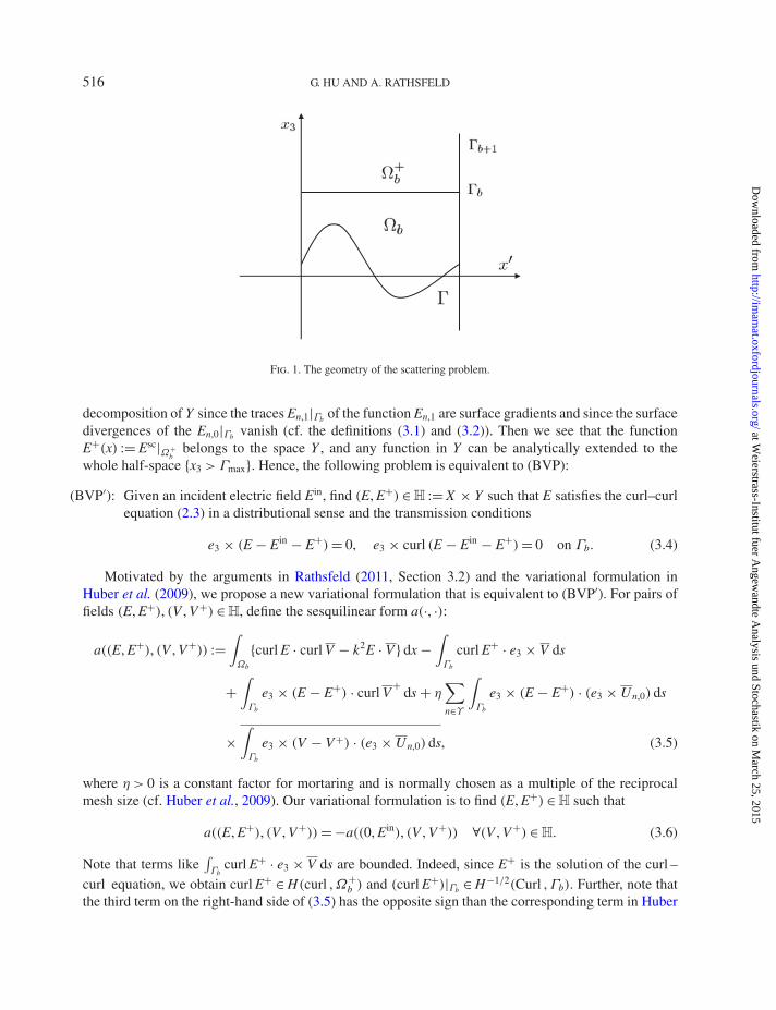
for x3 >Γmax (cf. also Rathsfeld, 2011, Section 2.5). Define the layer Ω+b above Γb of height one by

Ω+b := {x ∈ R

3 : 0< xj <Λj, j = 1, 2, b< x3 < b + 1} (cf. Fig. 1), and spaces Yl by

Yl := {U ∈ H(curl ,Ω+b ) : U(x)=

∑n∈Z2

Cn,lUn,l(x), Cn,l ∈ C}, l = 0, 1.

The spaces Y0, Y1 and Y := Y0 ⊕ Y1 are closed subspaces of the Sobolev space H(curl ,Ω+b ) (cf. the

subsequent orthogonality relations (4.7) and (4.8)). Moreover, the splitting Y = Y0 ⊕ Y1 is the Hodge


ngewandte A


http://imam


ownloaded from



Fig. 1. The geometry of the scattering problem.

decomposition of Y since the traces En,1|Γb of the function En,1 are surface gradients and since the surfacedivergences of the En,0|Γb vanish (cf. the definitions (3.1) and (3.2)). Then we see that the functionE+(x) := Esc|Ω+

bbelongs to the space Y , and any function in Y can be analytically extended to the

whole half-space {x3 >Γmax}. Hence, the following problem is equivalent to (BVP):

(BVP′): Given an incident electric field Ein, find (E, E+) ∈ H := X × Y such that E satisfies the curl–curlequation (2.3) in a distributional sense and the transmission conditions

e3 × (E − Ein − E+)= 0, e3 × curl (E − Ein − E+)= 0 on Γb. (3.4)

Motivated by the arguments in Rathsfeld (2011, Section 3.2) and the variational formulation inHuber et al. (2009), we propose a new variational formulation that is equivalent to (BVP′). For pairs offields (E, E+), (V , V+) ∈ H, define the sesquilinear form a(·, ·):

a((E, E+), (V , V+)) :=∫Ωb

{curl E · curl V − k2E · V } dx −∫Γb

curl E+ · e3 × V ds

+∫Γb

e3 × (E − E+) · curl V+

ds + η∑n∈Υ

∫Γb

e3 × (E − E+) · (e3 × Un,0) ds

×∫Γb

e3 × (V − V+) · (e3 × Un,0) ds, (3.5)

where η > 0 is a constant factor for mortaring and is normally chosen as a multiple of the reciprocalmesh size (cf. Huber et al., 2009). Our variational formulation is to find (E, E+) ∈ H such that

a((E, E+), (V , V+))= −a((0, Ein), (V , V+)) ∀(V , V+) ∈ H. (3.6)

Note that terms like∫Γb

curl E+ · e3 × V ds are bounded. Indeed, since E+ is the solution of the curl –curl equation, we obtain curl E+ ∈ H(curl ,Ω+

b ) and (curl E+)|Γb ∈ H−1/2(Curl ,Γb). Further, note thatthe third term on the right-hand side of (3.5) has the opposite sign than the corresponding term in Huber


ngewandte A


http://imam


ownloaded from



et al. (2009). Moreover, the integrals with factor η in (3.5) correspond to the following term involved inthe variational equation established in Huber et al. (2009):

η

∫Γb

e3 × (E − E+) · e3 × (V − V+) ds. (3.7)

The expression (3.7) is not meaningful for general (E, E+), (V , V+) ∈ H, since both e3 × (E − E+) ande3 × (V − V+) belong to H−1/2

t (Div ,Γb). Integrals like η∫Γb

e3 × u · e3 × v ds in the mortar approachmake sense for finite element methods, where u and v are finite element functions and η tends to zerowith the meshsize. The idea employed in Rathsfeld (2011) is to replace the integral (3.7) by the Galerkinapproximation

∑n,l:|n|2<Nβn |= 0 or l=0

η

∫Γb

e3 × (E − E+) · e3 × Un,l ds∫Γb

e3 × (V − V+) · e3 × Un,l ds (3.8)

+ η∑

n:βn=0

∫Γb

e3 × (E − E+) · Un,0 ds∫Γb

e3 × (V − V+) · Un,0 ds, (3.9)

with a sufficiently large number N > 0. It is also mentioned in Rathsfeld (2011) that the summation in(3.8) and (3.9) can even be restricted to all n ∈ Z

2 with βn = 0. In the present paper, we only use theterms of (3.8) with βn = 0, which are the last terms in (3.5).

To prove the equivalence of (3.6) and (BVP′), we need two lemmas.

Lemma 3.1 (i) We have curl Un,l = i(−1)lUn,1−l

√|αn|2 + |βn|21−2l

k2l, l = 0, 1.

(ii) Setting cos θn := βn/√

|βn|2 + |αn|2, there holds

e3 × Un,l|Γb =

⎧⎪⎨⎪⎩(−αn/|αn|, 0)� exp(iαn · x′) if n ∈Υ , l = 0,

(0, 0, 0)� if n ∈Υ , l = 1,

(−1)l[(e3 × Un,1−l)× e3](cos θn)2l−1 if n /∈Υ .

(iii) The following set is an L2-orthogonal basis of the space H−1/2t (Γb):

{e3 × Un,l|Γb : n /∈Υ , l = 0, 1} ∪ {e3 × Un,0|Γb : n ∈Υ } ∪ {Un,0|Γb : n ∈Υ }.

Proof. Lemma 3.1(i) and (ii) can be proved directly using the definitions of Un,l in (3.3). To provethe third assertion, we define the set Πn := {e3 × En,0, e3 × En,1} if βn |= 0 and Πn := {e3 × En,0, En,0} ifβn = 0 with En,l ∈ C

3 given in (3.1) and (3.2). Then Lemma 3.1(iii) simply follows from the definitionof H−1/2

t (Γb) and the fact that Πn spans the set {(a1, a2, 0)� : a1, a2 ∈ C} for any n ∈ Z2. �

In the following sections we make the convention that any sum over l is the sum over l = 0, 1.

Lemma 3.2 For any two absolutely convergent Rayleigh series expansion U and V defined in aneighborhood of Γb, there holds∫

Γb

(curl U)T · e3 × V ds =∫Γb

e3 × U · (curl [V ]mo)T ds,


ngewandte A


http://imam


ownloaded from



where [·]mo is a modification operator defined by⎡⎣∑

n∈Z2,l

Cn,lUn,l

⎤⎦

mo

:= −∑

l,n:βn>0

Cn,lUn,l +∑

l,n:βn /∈R

Cn,lUn,l.

Proof. See Rathsfeld (2011, Lemma 3.1). �

We are now going to prove:

Lemma 3.3 The variational formulation (3.6) and the problem (BVP′) are equivalent.

Proof. (i) Assume that (E, E+) ∈ H is a solution to (BVP′). Applying Green’s first vector theorem tothe region Ωb gives

0 =∫Ωb

{curl curl E − k2E} · V dx =∫Ωb

{curl E · curl V − k2E · V } dx −∫Γb

e3 × V · curl E ds

for any V ∈ X . Note that the integral over Γ vanishes due to the perfectly conducting boundary con-dition ν × V = 0 on Γ , and that the integrals over the vertical parts of ∂Ωb cancel because of theα-quasiperiodicity of V and E in Ωb. This implies that∫

Ωb

{curl E · curl V − k2E · V } dx =∫Γb

e3 × V · curl E ds, ∀V ∈ X . (3.10)

Making use of the identity (3.10) and the transmission conditions in (3.4), we derive from the definitionof the sesquilinear form a(·, ·) that

a((E, E+ + Ein), (V , V+))=∫Γb

curl (E − E+ − Ein) · e3 × V ds +∫Γb

e3 × (E − E+ − Ein) · curl V+

ds

+ η∑n∈Υ

∫Γb

e3 × (E − E+ − Ein) · (e3 × Un,0) ds

×∫Γb

e3 × (V − V+) · (e3 × Un,0) ds = 0 (3.11)

for any (V , V+) ∈ H, i.e., the pair (E, E+) is a solution to (3.6).(ii) Suppose that (E, E+) ∈ H is a solution to (3.6). Choose V ∈ X with a compact support in the

interior of Ωb (i.e. Supp(V)⊂ IntΩb) and choose V+ ≡ 0 in Y . Then,

0 = a((E, E+ + Ein), (V , 0))=∫Ωb

{curl E · curl V − k2E · V } dx =∫Ωb

(curl curl E − k2E) · V dx.

(3.12)This implies that curl curl E − k2E = 0 in Ωb. It remains to prove that only E and E+ satisfy the trans-mission conditions in (3.4).

Analogously to part (i), multiplying V ∈ X to the curl–curl equation curl curl E − k2E = 0 inΩb andthen using integration by parts yields the identity (3.10). Combining this identity with the variationalformulation (3.6) gives rise to the equality (3.11) for all (V , V+) ∈ H. By Lemma 3.1(ii) and (iii), we


ngewandte A


http://imam


ownloaded from



consider the Fourier expansion

(E − E+ − Ein)T =∑l,n/∈Υ

Cn,l(Un,l)T +∑n∈Υ

[Cn,0Un,0 + Cn,1e3 × Un,0] on Γb. (3.13)

It then suffices to prove that Cn,l = 0 for all n ∈ Z2, l = 0, 1. Indeed, (E − E+ − Ein)T = 0 on Γb together

with (3.11) for all V ∈ X would lead to (curl (E − E+ − Ein)|Γb)T = 0.First we take V ≡ 0 and V+ = Un,1 for some n ∈Υ in (3.11). Applying Lemma 3.1(i) to Un,1 gives

the identity curl V+ = −ikUn,0, and then, using e3 × Un,1 = 0 for n ∈Υ (cf. Lemma 3.1(ii)), we derivefrom (3.11) that ∫

Γb

e3 × (E − E+ − Ein) · Un,0 ds = 0 if n ∈Υ . (3.14)

Together with (3.13), this implies that Cn,1 = 0 for n ∈Υ .Next, inserting (3.14) into (3.11) with V ≡ 0 and using Lemma 3.2, we have

0 =∫Γb

e3 × (E − E+ − Ein) · curl V+

ds − η∑n∈Υ

∫Γb

(E − E+ − Ein)T · Un,0 ds∫Γb

V+T · Un,0 ds

=∫Γb

curl [(E − E+ − Ein|Γb)]mo · e3 × (V+) ds − η

∑n∈Υ

∫Γb

(E − E+ − Ein)T · Un,0 ds∫Γb

V+T · Un,0 ds

(3.15)

for all V+ ∈ Y , where the quantity

[(E − E+ − Ein)|Γb ]mo := −∑

l,n:βn>0

Cn,lUn,l +∑

l,n:βn /∈R

Cn,lUn,l on Γb

is obtained by firstly extending the series expansion (3.13) to a neighborhood of Γb and then applyingthe modification operator [·]mo of Lemma 3.2. From Lemma 3.1(i) and (ii), it follows that on Γb,

{curl [(E − E+ − Ein|Γb)]mo}T

=∑

n,l:βn>0

i(−1)l+1kCn,l(Un,1−l)T +∑

n,l:βn /∈R

i(−1)lk2lCn,l

√|αn|2 + |βn|2

1−2l(Un,1−l)T

=∑

n,l:βn>0

−ikCn,l(cos θn)1−2le3 × Un,l +

∑n,l:βn /∈R

ik2lCn,l(βn)1−2le3 × Un,l. (3.16)

Inserting (3.16) into (3.15) and choosing V+ = Un,l for some n /∈Υ , we derive Cn,l = 0. Analogously,the choice V+ = Un,0 for some n ∈Υ leads to Cn,0 = 0. This completes the proof. �

Remark 3.1 In the non-resonance case, i.e. Υ = ∅, the variational formulations (3.6) and (2.7) areequivalent. In fact, if (E, E+) is a solution to the problem (3.6), then by Lemma 3.3, the transmission


ngewandte A


http://imam


ownloaded from



conditions in (3.4) hold. Hence, we obtain

0 = a((E, E+ + Ein), (V , V+))=∫Ωb

curl E · curl V − k2E · V dx −∫Γb

curl (E+ + Ein) · e3 × V ds

=∫Ωb

curl E · curl V − k2E · V dx −∫Γb

R(e3 × E) · e3 × V ds

+∫Γb

[R(e3 × Ein)− curl Ein] · e3 × V ds,

which is equivalent to the variational formulation (2.7) involving the Dirichlet-to-Neumann map R.Note that in the last step of the previous identity we have used the identity (curl E+)T = R(e3 × E+)=R(e3 × E)− R(e3 × Ein) on Γb. On the other hand, supposing that E ∈ H(curl ,Ωb) is a solution to(2.7), we extend the scattered field Esc := E − Ein from Ωb to x3 > b by the Rayleigh expansion (2.5).Assume that the coefficients An are given by

e3 × Esc|Γ −b

= e3 × (E − Ein)|Γ −b

=∑n∈Z2

An eiαn·x′ ∈ H−1/2t (Div ,Γb), An ∈ C

3. (3.17)

Here and in the following, the symbol (·)|Γ −b

resp. (·)|Γ +b

denotes the trace obtained from below andabove Γb, respectively. It follows from the variational formulation (2.7) that e3 × curl Esc × e3|Γ −

b=

R(e3 × Esc|Γ −b). The extension of the series in (3.17) to the half space x3 > b in form of the Rayleigh

expansion (2.5) is

Esc(x)=∑n∈Z2

[An × e3 + β−1n (e3 × An) · αne3] eiαn·x′+iβn(x3−b), x3 > b.

Then, we obtain e3 × Esc|Γ −b

= e3 × Esc|Γ +b

and e3 × curl Esc × ye3|Γ +b

= R(e3 × Esc|Γ +b). Setting

E+ = Esc in Ω+b , we conclude that (E, E+) satisfies the transmission conditions (3.4) and thus is a

solution of (3.6).

4. Analysis of the variational formulation (3.6)

Since the sesquilinear form a(·, ·) defined in Section 3 is bounded on H, it obviously generates a con-tinuous linear operator A : H → H

′ satisfying

a((E, E+), (V , V+))= 〈A(E, E+), (V , V+)〉Ωb×Ω+b

. (4.1)

Here H′ denotes the dual of the space H with respect to the duality 〈·, ·〉Ωb×Ω+

bextending the scalar

product in L2(Ωb)3 × L2(Ω+

b )3. The aim of this section is to prove the following theorem:

Theorem 4.1 The operator A defined by (4.1) is a Fredholm operator with index zero.

To prove Theorem 4.1, we need several auxiliary lemmas. We first prove a periodic analogue of theHodge-decomposition of X , following the argument in Monk (2003, Theorem 4.3). See also Abboud(1993), Ammari (1995), Ammari & Bao (2008) and Hu et al. (2010) for other Hodge-decompositionsof the Sobolev spaces in periodic structures. Define the subspaces X1 := {∇p : p ∈ H1(Ωb), p = 0 on Γ }and X0 := {E0 ∈ X :

∫Ωb

∇p · E0 dx = 0∀ ∇p ∈ X1}.


ngewandte A


http://imam


ownloaded from



Lemma 4.1 We have X = X0 ⊕ X1 with the subspaces X0 and X1 orthogonal in L2(Ωb)3 and H(curl,Ωb).

Moreover, div E0 = 0 and (e3 · E0)|Γb = 0 for any E0 ∈ X0, and X0 is compactly embedded into L2(Ωb)3.

Proof. Define the sesquilinear form b(E, V) := ∫Ωb

{curl E · curl V + E · V } dx for all E, V ∈ X . Then,for ∇p ∈ X1, we obtain b(∇p, ∇p)= ‖∇p‖2

L2(Ωb)= ‖∇p‖2

X . Thus, for every E ∈ X , there exists a uniquesolution ∇p ∈ X1 such that

b(∇p, ∇ξ)= b(E, ∇ξ), ∀ ∇ξ ∈ X1. (4.2)

Let E0 := E − ∇p. Using integration by parts and the quasiperiodicity of E0 and ξ in Ωb, (4.2) implies

0 =∫Ωb

E0 · ∇ξ dx = −∫Ωb

ξ div E0 dx +∫Γb

ξe3 · E0 ds, ∀ ∇ξ ∈ X1.

Consequently, X = X1 + X0 and div E0 = 0, (e3 · E0)|Γb = 0. On the other hand, if ∇q ∈ X0 ∩ X1, thenthe definition of X0 implies that

∫Ωb

∇p · ∇q dx = 0. Setting p = q, we get ∇q = 0, i.e., X0 ∩ X1 = ∅.Finally, the compact imbedding of X0 into L2(Ωb)

3 follows from Monk (2003, Corollary 3.49) (see alsoAmmari & Bao, 2008, Lemma 3.2). �

By Lemma 4.1 and the definitions of Yl, we can decompose our space H into four subspaces. For(E, E+), (V , V+) ∈ H, we may assume that

E = ∇p + E0, E+ = E+0 + E+

1 where ∇p ∈ X1, E0 ∈ X0, E+l ∈ Yl, l = 1, 2,

V = ∇ξ + V0, V+ = V+0 + V+

1 where ∇ξ ∈ X1, V0 ∈ X0, V+l ∈ Yl, l = 1, 2.

To analyse the form a, we define several sesquilinear forms aj with j = 1, 2, . . . , 6. Let

a1(∇p, ∇ξ) := k2∫Ωb

∇p · ∇ξ dx, ∀ ∇p, ∇ξ ∈ X1,

a2(E0, V0) :=∫Ωb

{curl E0 · curl V0 − k2E0 · V0} dx, ∀ E0, V0 ∈ X0,

a3(E+0 , V+

0 ) :=∫Γb

e3 × E+0 · curl V

+0 ds, ∀ E+

0 , V+0 ∈ Y0,

a4(E+1 , V+

1 ) :=∫Γb

e3 × E+1 · curl V

+1 ds, ∀ E+

1 , V+1 ∈ Y1

and let

a5((E, E+), (V , V+)) := a5(E, V+) :=∫Γb

e3 × E · curl V+

ds,

a6((E, E+), (V , V+)) := η∑n∈Υ

{∫Γb

e3 × (E − E+) · (e3 × Un,0) ds∫Γb

e3 × (V − V+) · (e3 × Un,0) ds

}(4.3)

for any (E, E+), (V , V+) ∈ H.

Lemma 4.2 For any ∇ξ ∈ X1 and V+0 ∈ Y0, we have a5(∇ξ , V+

0 )= 0.


ngewandte A


http://imam


ownloaded from



Proof. From the definition of Y and Y0 we conclude that Y0 is in the subspace of all vector functionsV+ ∈ Y with e3 · V+ = 0. Therefore it suffices to prove∫

Γb

[e3 × ∇ξ ] · curl V+

ds = k2∫Γb

e3 · V+ξ ds. (4.4)

Note that the right-hand side of (4.4) is a continuous functional of V+ and ξ . Indeed, from V+ ∈ L2(Ω+b )

and 0 = ∇ · V+ ∈ L2(Ω+b ), we conclude e3 · V

+|Γb ∈ H−1/2(Γb), and ξ ∈ H1/2(Γb) follows from ξ ∈H1(Ωb). Knowing the continuity, it suffices to prove (4.4) for a dense subset, e.g., for a truncatedRayleigh expansion V+ and smooth ξ . We conclude∫

Γb

[e3 × ∇ξ ] · curl V+

ds = −∫Γ

[ν × ∇ξ ] · curl V+

ds +∫Ωb

[curl ∇ξ ] · curl V+

ds

−∫Ωb

[∇ξ ] · curl curl V+

ds = k2∫Ωb

[∇ξ ] · V+

ds,

where we have used that the tangential derivative ν × ∇ξ of the function ξ with ξ |Γ = 0 vanishes. Using∇ · V+ = 0, we continue

k2∫Ωb

[∇ξ ] · V+

ds = k2∫Ωb

∇ · [ξV+

] ds = k2∫Γb

ξe3 · V+

ds + k2∫Γ

ξν · V+

ds = k2∫Γb

ξe3 · V+

ds

and the proof is completed. �

Using Lemmas 3.1, 4.1 and 4.2, it follows from the definition of a that (see Table 1)

a((E, E+), (V , V+))

= a((∇p + E0, E+0 + E+

1 ), (∇ξ + V0, V+0 + V+

1 ))

=∫Ωb

{curl E0 · curl V 0 − k2E0 · V 0 − k2∇p · ∇ξ} dx −∫Γb

curl E+0 · e3 × V 0 dx

−∫Γb

curl E+1 · e3 × V 0 dx −

∫Γb

curl E+1 · e3 × ∇ξ dx +

∫Γb

e3 × E0 · curl V+0 dx

+∫Γb

e3 × E0 · curl V+1 dx +

∫Γb

e3 × ∇p · curl V+1 dx −

∫Γb

e3 × E+0 · curl V

+0 dx

−∫Γb

e3 × E+1 · curl V

+1 dx + a6((E, E+), (V , V+))

= −a1(∇p, ∇ξ)+ a2(E0, V0)− a3(E+0 , V+

0 )− a4(E+1 , V+

1 )+ a5(E0, V+0 )− a5(V0, E+

0 )+ a5(E0, V+1 )

− a5(V0, E+1 )+ a5(∇p, V+

1 )− a5(∇ξ , E+1 )+ a6((E, E+), (V , V+)).

Definition 4.2 A bounded sesquilinear form l(·, ·) on a Hilbert space X is called strongly ellipticif there exists a compact form l(·; ·) and a constant c> 0 such that Re l(u, u)� c‖u‖2

X − l(u, u) forall u ∈ X .


ngewandte A


http://imam


ownloaded from



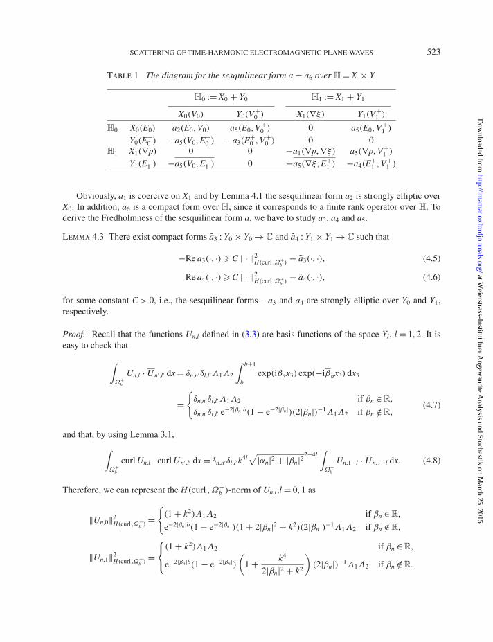
Table 1 The diagram for the sesquilinear form a − a6 over H = X × Y

H0 := X0 + Y0 H1 := X1 + Y1

X0(V0) Y0(V+0 ) X1(∇ξ) Y1(V

+1 )

H0 X0(E0) a2(E0, V0) a5(E0, V+0 ) 0 a5(E0, V+

1 )

Y0(E+0 ) −a5(V0, E+

0 ) −a3(E+0 , V+

0 ) 0 0H1 X1(∇p) 0 0 −a1(∇p, ∇ξ) a5(∇p, V+

1 )

Y1(E+1 ) −a5(V0, E+

1 ) 0 −a5(∇ξ , E+1 ) −a4(E

+1 , V+

1 )

Obviously, a1 is coercive on X1 and by Lemma 4.1 the sesquilinear form a2 is strongly elliptic overX0. In addition, a6 is a compact form over H, since it corresponds to a finite rank operator over H. Toderive the Fredholmness of the sesquilinear form a, we have to study a3, a4 and a5.

Lemma 4.3 There exist compact forms a3 : Y0 × Y0 → C and a4 : Y1 × Y1 → C such that

−Re a3(·, ·)� C‖ · ‖2H(curl ,Ω+

b )− a3(·, ·), (4.5)

Re a4(·, ·)� C‖ · ‖2H(curl ,Ω+

b )− a4(·, ·), (4.6)

for some constant C> 0, i.e., the sesquilinear forms −a3 and a4 are strongly elliptic over Y0 and Y1,respectively.

Proof. Recall that the functions Un,l defined in (3.3) are basis functions of the space Yl, l = 1, 2. It iseasy to check that

∫Ω+

b

Un,l · Un′,l′ dx = δn,n′δl,l′Λ1Λ2

∫ b+1

bexp(iβnx3) exp(−iβnx3) dx3

={δn,n′δl,l′Λ1Λ2 if βn ∈ R,

δn,n′δl,l′ e−2|βn|b(1 − e−2|βn|)(2|βn|)−1Λ1Λ2 if βn /∈ R,(4.7)

and that, by using Lemma 3.1,∫Ω+

b

curl Un,l · curl Un′,l′ dx = δn,n′δl,l′k4l√

|αn|2 + |βn|22−4l

∫Ω+

b

Un,1−l · Un,1−l dx. (4.8)

Therefore, we can represent the H(curl ,Ω+b )-norm of Un,l,l = 0, 1 as

‖Un,0‖2H(curl ,Ω+

b )={(1 + k2)Λ1Λ2 if βn ∈ R,

e−2|βn|b(1 − e−2|βn|)(1 + 2|βn|2 + k2)(2|βn|)−1Λ1Λ2 if βn /∈ R,

‖Un,1‖2H(curl ,Ω+

b )=⎧⎨⎩(1 + k2)Λ1Λ2 if βn ∈ R,

e−2|βn|b(1 − e−2|βn|)(

1 + k4

2|βn|2 + k2

)(2|βn|)−1Λ1Λ2 if βn /∈ R.


ngewandte A


http://imam


ownloaded from



On the other hand, using simple calculations, we have, for n /∈Υ ,∫Γb

e3 × Un,l · curl Un,l ds = (−i)(cos θn)2l−1k2l

√|αn|2 + |βn|2

1−2l∫Γb

|e3 × Un,1−l|2 ds,

by Lemma 3.1(i) and (ii). Furthermore,

∫Γb

|e3 × Un,1−l|2 ds ={

|eiβnb|2Λ1Λ2 if l = 1,

|eiβnb|2Λ1Λ2| cos θn|2 if l = 0,

by the definitions of Un,l given in (3.3). Combining the previous two equalities yields

Re∫Γb

e3 × Un,1 · curl Un,1 ds =⎧⎨⎩

0 if βn ∈ R,|βn|k2

2|βn|2 + k2e−2|βn|bΛ1Λ2 if βn /∈ R,

Re∫Γb

e3 × Un,0 · curl Un,0 ds ={

0 if βn ∈ R,

−|βn| e−2|βn|bΛ1Λ2 if βn /∈ R.

Since |βn| ∼√

1 + |n|2 as |n| → +∞, there holds

−Re∫Γb

e3 × Un,0 · curl Un,0 ds � C‖Un,0‖2H(curl ,Ωb)

, (4.9)

Re∫Γb

e3 × Un,1 · curl Un,1 ds � C‖Un,1‖2H(curl ,Ωb)

, (4.10)

whenever βn /∈ R, with C> 0 being a constant independent of l and n. Therefore, given the field E+0 =∑

n∈Z2 Cn,0Un,0 ∈ Y0, we deduce from (4.9) that

−Re a3(E+0 , E+

0 )= −∑n∈Z2

|Cn,0|2 Re∫Γb

e3 × Un,0 · curl Un,0 ds

� C∑βn /∈R

|Cn,0|2‖Un,0‖2H(curl ,Ω+

b )= C‖E+

0 ‖2H(curl ,Ω+

b )− a3(E

+0 , E+

0 ),

a3(E+0 , E+

0 ) := C∑βn∈R

|Cn,0|2‖Un,0‖2H(curl ,Ω+

b ).

Since the set {n ∈ Z2 : βn ∈ R} consists of a finite number of indices, the form a3(·, ·) : Y0 × Y0 → R is

compact. Thus the sesquilinear form −a3 is strongly elliptic over Y0. The proof for a4 can be carried outanalogously by employing (4.10). �

Remark 4.1 For the component-wise gradient ∇Un,l, the definition of Un,l leads to∫Ω+

b

|∇Un,l|2 dx = (|αn|2 + |βn|2)∫Ω+

b

|Un,l|2 dx. (4.11)


ngewandte A


http://imam


ownloaded from



Thus, comparing (4.11) with (4.8) leads to ‖Un,0‖2H1(Ω+

b )3 = ‖Un,0‖2

H(curl ,Ω+b )

. This implies that the H1-

and H(curl )-norm of the elements from Y0 are identical, i.e., ‖E+0 ‖H1(Ω+

b )3 = ‖E+

0 ‖H(curl ,Ω+b )

, if E+0 ∈ Y0.

However, this is not true for the space Y1.

We turn to the properties of a5 defined in (4.3).

Lemma 4.4 The sesquilinear form a5 is compact over X0 × Y1.

Proof. For V+1 ∈ Y1 ⊂ Y , define the operator J(V+

1 ) := curl V+1 . Obviously, we get ‖J(V+

1 )‖2L2(Ω+

b )3 �

‖V+1 ‖2

H(curl ,Ω+b )

, and curl J(V+1 )− k2V+

1 = 0 implies ‖curl J(V+1 )‖2

L2(Ω+b )

3 � k2‖V+1 ‖2

H(curl ,Ω+b )

. Hence, by

Lemma 3.1(i), J is a bounded linear map from Y1 into Y0. In view of the equivalence of the norms‖JV+

1 ‖H(curl ,Ω+b )

and ‖JV+1 ‖H1(Ω+

b )3 (see Remark 4.1), we see that J is also bounded from the subspace

Y1 of H(curl ,Ω+b ) into the subspace Y0 of H1(Ω+

b )3, with the trace J(V+

1 )|Γb ∈ H1/2(Γb)3. Thus, there

exists an extension W of (curl V+1 )|Γb from H1/2(Γb)

3 into H1(Ωb)3 such that W = curl V+

1 on Γb andν × W = 0 on Γ . Using integration by parts,

a5(E0, V+1 )=

∫Γb

e3 × E0 · J(V+) ds =∫Γb

e3 × E0 · W ds =∫Ωb

{curl E0 · W − E0 · curl W} dx.

From the compact embedding of W ∈ H1(Ωb)3 into L2(Ωb)

3 and that of E0 ∈ X0 into L2(Ωb)3, it follows

that the sesquilinear form a5(E0, V+1 ) is compact over X0 × Y1. �

Combining Lemmas 4.1, 4.2, 4.3 and 4.4, we are now in a position to prove the Fredholm propertyof the variational formulation (3.6).

Proof of Theorem 4.1. It suffices to verify that the sesquilinear form a − a6 is Fredholm over H withindex zero. To do this, we define the spaces Hj = Xj ⊕ Yj for j = 0, 1, so that we can rewrite H = X ×Y = H0 × H1. Define the sesquilinear forms:

b0((E0, E+0 ), (V0, V+

0 )) := a2(E0, V0)− a3(E+0 , V+

0 )+ a5(E0, V+0 )− a5(V0, E+

0 ),

b1((∇p, E+1 ), (∇ξ , V+

1 )) := −a1(∇p, ∇ξ)− a4(E+1 , V+

1 )+ a5(∇p, V+1 )− a5(∇ξ , E+

1 ),

for all (E0, E+0 ), (V0, V+

0 ) ∈ H0 and for all (∇p, E+1 ), (∇ξ , V+

1 ) ∈ H1, respectively. Now split the formin Table 1 in blocks corresponding to the splitting H = H0 × H1. Then the restriction to H0 is theform b0 with the strongly elliptic quadratic form Re b0((E0, E+

0 ), (E0, E+0 ))= a2(E0, E0)− a3(E

+0 , E+

0 ).The restriction to H1 is the form b1, and the sesquilinear form −b1 has the strongly elliptic quadraticform −Re b1((∇p, E+

1 ), (∇p, E+1 ))= a1(∇p, ∇p)+ a4(E

+1 , E+

1 ). Consequently, the diagonal blocks ofthe 2 × 2 splitting correspond to Fredholm operators with index zero. On the other hand, the full formin Table 1 differs from the diagonal block matrix only by compact terms. Hence the form a generates aFredholm operator with index zero. �

5. Proof of Theorem 2.1

Since the problem (BVP′) and (3.6) are equivalent (see Lemma 3.3), to prove Theorem 2.1 we onlyneed to show the existence of solutions to (3.6) with Ein replaced by Ein

gen given in (2.6). Consider the


ngewandte A


http://imam


ownloaded from



homogeneous adjoint problem of the variational formulation (3.6): find (V , V+) ∈ H such that

a((W , W+), (V , V+))= 0 (5.1)

for all (W , W+) ∈ H. By Fredholm’s alternative, it suffices to verify a((0, Eingen), (V , V+))= 0 for any

solution (V , V+) to (5.1). The following lemma describes properties of the solution (V , V+), which willbe used later for proving Theorem 2.1.

Lemma 5.1 Assume that (V , V+) ∈ H is a solution to the homogeneous adjoint problem (5.1). Then

VT |Γb , (curl V+)T |Γb ∈ Span{{(Un,l)T |Γb : βn /∈ R, l = 1, 2} ∪ {Un,0|Γb : βn = 0}}. (5.2)

Proof. Analogous to the proof of (3.12), one can prove that curl curl V − k2V = 0 holds in Ωb, leadingto the identity (3.10) with (V , E) replaced by (W , V). By the definition of a(·, ·),

0 = a((W , W+), (V , V+))

=∫Γb

{e3 × W · curl V − curl W+ · e3 × V } ds +∫Γb

e3 × (W − W+) · curl V+

ds

+ η∑n∈Υ

∫Γb

e3 × (W − W+) · e3 × Un,0 ds∫Γb

e3 × (V − V+) · e3 × Un,0 ds (5.3)

for all (W , W+) ∈ H. In the following we will prove (5.2) choosing different test functions (W , W+) ∈H.

(i) Choose W ≡ 0, W+ = Un,0 for some n ∈Υ in (5.3). Since (curl Un,0|Γb)T = 0 on Γb

(cf. Lemma 3.1), simple calculations lead to∫Γb

[curl V+ + ηΛ1Λ2e3 × (V − V+)] · e3 × Un,0 ds = 0.

However, one can verify, using Lemma 3.1(i) and (ii), that∫Γb

{curl V+ · e3 × Un,0} ds = 0 for V+ ∈ Y .Hence, ∫

Γb

e3 × (V − V+) · e3 × Un,0 ds = 0 if n ∈Υ . (5.4)

(ii) Choose W ≡ 0 and W+ = Un,1 for some n ∈Υ in (5.3). Making use of e3 × Un,1 = 0 for n ∈Υ , wederive from (5.3) that

∫Γb

{curl Un,1 · e3 × V } ds = 0. This together with Lemma 3.1(i) gives the relation

∫Γb

{e3 × V · Un,0} ds = 0 if n ∈Υ . (5.5)

(iii) Inserting (5.4) and (5.5) into (5.3) with W ≡ 0 and taking into account Lemma 3.2, we obtain∫Γb

{curl [V ]mo + curl V+} · e3 × W+ ds = 0 for all W+ ∈ Y . By Lemma 3.1(iii), the last identity impliesthat

{(curl [V ]mo)T + (curl V+)T }|Γb ∈ Span{Un,0 : n ∈Υ }. (5.6)

Since V+ ∈ Y , we have curl V+ ∈ H(curl ,Ω+b ) and thus the trace (curl V+|Γb)T belongs to

H−1/2t (Curl ,Γb). Using Lemma 3.1(iii), we may assume that on Γb

(curl V+)T =∑

n:βn=0

{Bn,0Un,0 + Bn,1 e3 × Un,0} +∑

l,n:βn |= 0

Bn,l e3 × Un,l


ngewandte A


http://imam


ownloaded from



with Bn,l ∈ C. Combining the previous two formulas, we deduce from the definition of the modificationoperator [·]mo in Lemma 3.2 that (curl [V ]mo)T +∑l,n:βn |= 0 Bn,l e3 × Un,l = 0 on Γb and that Bn,1 = 0 forβn = 0. Therefore,

(curl V+)T =∑

n:βn=0

Bn,0Un,0 − (curl [V ]mo)T on Γb. (5.7)

(iv) Inserting (5.4) and (5.5) into (5.1) with W+ = 0 and W = V , we find (cf. (3.5) with E+ ≡ 0 andE = V )

0 = Im a((V , 0), (V , V+))= Im∫Γb

e3 × V · (curl V+)T ds, (5.8)

where the function (curl V+)T |Γb is given in (5.7). According to Lemma 3.1(iii), we may represente3 × V |Γb as

e3 × V =∑

l,n:βn |= 0

Cn,le3 × Un,l +∑

n:βn=0

{Cn,0e3 × Un,0 + Cn,1Un,0}, Cn,l ∈ C,

on Γb. However, by (5.5) there holds Cn,1 = 0 for n ∈Υ . Thus, applying Lemma 3.1 gives

e3 × V =∑

l,n:βn |= 0

Cn,l(−1)l(Un,1−l)T (cos θn)2l−1 +

∑n:βn=0

Cn,0e3 × Un,0 on Γb, (5.9)

(curl [V ]mo)T = −∑

l,n:βn>0

Cn,l(curl Un,l)T +∑

l,n:βn /∈R

Cn,l(curl Un,l)T

= −∑

l,n:βn>0

i(−1)lkCn,l(Un,1−l)T +∑

l,n:βn /∈R

i(−1)l√

|αn|2 + |βn|21−2l

k2lCn,l(Un,1−l)T

(5.10)

on Γb. Inserting the above identity (5.10) into (5.7) and using (5.9), we derive from (5.8) that

0 = Im

⎧⎨⎩−ik

∑l,n:βn>0

|Cn,l|2‖(Un,1−l)T‖2L2(Γb)

(cos θn)2l−1

⎫⎬⎭

+ Im

⎧⎨⎩−

∑l,n:βn /∈R

|Cn,l|2(ik)2l‖(Un,1−l)T‖2L2(Γb)

|βn|1−2l[|αn|2 + |βn|2]1−2l

⎫⎬⎭

= −k∑

l,n:βn>0

|Cn,l|2‖(Un,1−l)T‖2L2(Γb)

(cos θn)2l−1,

which, together with the definition of cos θn in Lemma 3.1, leads to

Cn,l = 0 for all βn > 0, l = 1, 2. (5.11)

Finally, combining (5.11) and (5.9) we have proved (5.2) for VT |Γb , and combining (5.11), (5.10) and(5.7) leads to the desired result for (curl V+|Γb)T . �


ngewandte A


http://imam


ownloaded from



We proceed to prove Theorem 2.1, i.e., to show the existence of a solution (E, E+) ∈ H to the varia-tional problem (3.6) for the incident wave Ein

gen. Assume (V , V+) ∈ H satisfies a((W , W+), (V , V+))= 0for all (W , W+) ∈ H. Using Lemmas 5.1 and 3.1, it is easy to check that

a((0, Eingen), (V , V+))= −

∫Γb

{curl Eingen · e3 × V + e3 × Ein

gen · curl V+} ds = 0. (5.12)

This means that each solution to the homogeneous adjoint problem (5.1) is orthogonal to the right-hand side of the variational problem (3.6) in the sense of (5.12). According to Theorem 4.1, the Fred-holm alternative applied to the variational problem (3.6) yields the existence of the solution (E, E+) ∈ H

to problem (3.6) for the incident plane waves Eingen defined in (2.6).

Formula (5.2) implies that solution V+ takes the form V+(x)=∑βn /∈RCn,lUn,l(x)+∑

βn=0 Cn,lUn,l(x) for x ∈Ω+b . Thus V+ ∈ Y and the coefficients of the propagating modes for

βn > 0 vanish. By analogous arguments, this assertion even remains valid for the solution (V , V+)to the homogeneous variational problem a((V , V+), (W , W+))= 0 for all (W , W+) ∈ H. In otherwords, the coefficient Cn,l of the difference of two solutions of (BVP) are zero if βn > 0. The proof ofTheorem 2.1 is thus completed.

Acknowledgement

The authors would like to thank their colleague J. Elschner for pointing out the research articles (Gotlib,2000; Kamotski & Nazarov, 2002) which stimulated this paper.

Funding

This research was supported by the German Research Foundation (DFG) under Grant No. EL 584/1-2(to G.H.).

References

Abboud, T. (1993) Formulation variationnelle des équations de Maxwell dans un réseau bipériodique de R3. C. R.

Acad. Sci. Pairs, 317, 245–248.Ammari, H. (1995) Uniqueness theorems for an inverse problem in a doubly periodic structure. Inv. Probl., 11,

823–833.Ammari, H. & Bao, G. (2008) Coupling of finite element and boundary element methods for the scattering by

periodic chiral structures. J. Comput. Math., 3, 261–283.Bao, G. (1997) Variational approximation of Maxwell’s equation in biperiodic structures. SIAM J. Appl. Math., 57,

364–381.Bao, G., Cowsar, L. & Masters, W. (eds) (2001) Mathematical Modeling in Optical Science. Frontiers in Applied

Mathematics. SIAM Series. Philadelphia: SIAM.Bao, G. & Dobson, D. C. (2000) On the scattering by biperiodic structures. Proc. Amer. Math. Soc., 128,

2715–2723.Bonnet-Bendhia, A. S. & Starling, F. (1994) Guided waves by electromagnetic gratings and non-uniqueness

examples for the diffraction problem. Math. Meth. Appl. Sci., 17, 305–338.Buffa, A., Costabel, M. & Sheen, D. (2002) On traces for H(curl ,Ω) in Lipschitz domains. J. Math. Anal. Appl.,

276, 847–867.Chen, X. & Friedman, A. (1991) Maxwell’s equations in a periodic structure. Trans. AMS, 323, 465–507.Colton, D. & Kress, R. (1998) Inverse Acoustic and Electromagnetic Scattering Theory. Berlin: Springer.


ngewandte A


http://imam


ownloaded from



Dobson, D. C. (1994) A variational method for electromagnetic diffraction in biperiodic structures. RAIRO Model.Math. Anal. Numer, 28, 419–439.

Elschner, J. & Hu, G. (2010) Variational approach to scattering of plane elastic waves by diffraction gratings.Math. Meth. Appl. Sci, 33, 1924–1941.

Elschner, J. & Schmidt, G. (1998) Diffraction in periodic structures and optimal design of binary gratings I.Direct problems and gradient formulas. Math. Methods Appl. Sci., 21, 1297–1342.

Gohberg I. C. & Krein, M. G. (1969) Introduction to the Theory of Linear Nonselfadjoint Operators in HilbertSpace. Translations of Mathematical Monographs, vol. 18. Providence, RI: American Mathematical Society.

Gotlib, V. Yu. (2000) Solutions of the Helmholtz equation, concentrated near a plane periodic boundary. J. Math.Sci., 102, 4188–4194.

Haddar, H. & Lechleiter, A. (2011) Electromagnetic wave scattering from rough penetrable layers. SIAMJ. Math. Anal., 43, 2418–2443.

Hiptmaier, R. (2012) Coupling of finite elements and boundary elements in electromagnetic scattering. SIAMJ. Numer. Anal., 41, 919–944.

Hu, G., Qu, F. & Zhang, B. (2010) Direct and inverse problems for electromagnetic scattering by a doubly periodicstructure with a partially coated dielectric. Math. Methods Appl. Sci., 33, 147–156.

Hu, G. & Rathsfeld, A. (2012) Convergence analysis of the FEM coupled with Fourier-mode expansion for theelectromagnetic scattering by biperiodic structures. WIAS preprint, no. 1744, Berlin.

Hu, G., Yang, J. & Zhang, B. (2009) Inverse electromagnetic scattering for a biperiodic inhomogeneous layer onperfectly conducting plates. Appl. Anal., 90, 317–333.

Huber, M., Schoeberl, J., Sinwel, A. & Zaglmayr, S. (2009) Simulation of diffraction in periodic media witha coupled finite element and plane wave approach. SIAM J. Sci. Comput., 31, 1500–1517.

Kamotski, I. V. & Nazarov, S. A. (2002) The augmented scattering matrix and exponentially decaying solutionsof an elliptic problem in a cylindrical domain. J. Math. Sci., 111, 3657–3666.

Kleemann, B. (2002) Elektromagnetische Analyse von Oberflächengittern von IR bis XUV mittels einerparametrisierten Randintegralmethode: Theorie, Vergleich und Anwendungen. Dissertation, Technischen Uni-versität Ilmenau.

Li, P., Wu, H. & Zheng, W. (2011) Electromagnetic scattering by unbounded rough surfaces. SIAM J. Math. Anal.,43, 1205–1231.

Monk, P. (2003) Finite element method for Maxwell’s equations, Oxford: Oxford University Press.Nédélec, J. C. & Starling, F. (1991) Integral equation methods in a quasi-periodic diffraction problem for the

time-harmonic Maxwell equation. SIAM J. Math. Anal., 22, 1679–1701.Nitsche, J. (1970) Über ein Variationsprinzip zur Lösung von Dirichlet-Problemen bei Verwendung von Teilräu-

men. Abh. Math. Sem. Univ. Hamburg, 36, 9–15.Rathsfeld, A. (2013) Shape derivatives for the scattering by biperiodic gratings. Appl. Numer. Math., 72, 19–32.Schmidt, G. (2003) On the diffraction by biperiodic anisotropic structures. Applicable Anal., 82, 75–92.Schmidt, G. (2004) Electromagnetic scattering by periodic structures. J. Math. Sci., 124, 5390–5405.Sternberg, R (1988) Mortaring by a method of J. A. Nitsche, Computational Mechanics, New Trends and Appli-

cations (S. Idelsohn, E. Onate, E. Dvorkin eds). Spain: CIMNE Barcelona.Turunen, J., Kuittinen, M. & Wyrowski, F. (2000) Diffractive optics: electromagnetic approach. Progress in

Optics XL (E. Wolf ed.). Amsterdam: Elsevier Science B. V., pp. 343–388.Turunen, J. & Wyrowski, F. (eds) (2003) Diffractive Optics for Industrial and Commercial Applications. Berlin:

Akademie.

Appendix

For the reader’s convenience, we prove that the variational formulation (2.7) is uniquely solvable forsmall wavenumbers k > 0. Since Rayleigh frequencies can be excluded for small wavenumbers, by


ngewandte A


http://imam


ownloaded from



Remark 3.1 we see that such a unique solvability also applies to our variational formulation (3.6)provided k is sufficiently small.

Lemma A.1 There is a k0 > 0 such that the variational formulation (2.7) admits a unique solution E ∈ Xfor all wavenumbers k with 0< k � k0.

Proof. To prove Lemma A.1, we need to replace equation (2.7) on the k-dependent α-quasi-periodicspace H(curl ,Ωb) by an equivalent variational problem acting on the (Λ1,Λ2)-periodic Sobolev space.Introduce the spaces H1

p (Ωb), Hp(curl ,Ωb), Hst,p(Γb), Hs

t,p(Div ,Γb) and Hst,p(Curl ,Γb) in the same way

as H1(Ωb), H(curl ,Ωb), Hst (Γb), Hs

t (Div ,Γb) and Hst (Curl ,Γb) in Section 2, but with α= (0, 0)�. Fur-

thermore, define the operator ∇α := ∇ + i(α, 0)� and, analogously to the space X defined in Section 2,set D := {F :Ωb → C

3, F ∈ Hp(curl ,Ωb), ν × F = 0 on Γ }. Let τn := (2πn1/Λ1, 2πn2/Λ2)� = αn − α

for n = (n1, n2)� ∈ Z

2. Given

F(x′)=∑n∈Z2

Fn eiτn·x′ ∈ H−1/2t,p (Div ,Γb), (A.1)

the definition of the operator R (cf. (2.8)) implies R(E)= T (F) exp(iα · x′) for E(x′)= eiα·x′F(x′) ∈

H−1/2t (Div ,Γb), where the operator T : H−1/2

t,p (Div ,Γb)→ H−1/2t,p (Curl ,Γb) is the Dirichlet-to-

Neumann map over the space H−1/2t,p (Div ,Γb) defined by

(T F)(x′)= −∑n∈Z2

1

iβn[k2Fn − (αn · Fn)αn] exp(iτn · x′), n = (n1, n2)

� ∈ Z2. (A.2)

Note that T is well defined for small wavenumbers k with 0< k � k0, since βn |= 0 if k0 is sufficientlysmall. The spaces H−1/2

t,p (Γb), H−1/2t,p (Div ,Γb) and H−1/2

t,p (Curl ,Γb) will be equipped with the normsanalogous to the quasi-periodic ones in Section 2, but with the coefficient En replaced by Fn given in(A.1) and αn replaced by τn.

Set Fin(x) := exp(−iα · x′)Ein(x), F(x)= exp(−iα · x′)E(x), as well as ψ(x)= exp(−iα · x′)ϕ(x) ∈Hp(curl ,Ωb) for E,ϕ ∈ H(curl ,Ωb). We now consider the variational formulation

ap(F,ψ) :=∫Ωb

[∇α × F · ∇α × ψ − k2F · ψ] dx −∫Γb

T (e3 × F) · (e3 × ψ) ds

=∫Γb

[(∇α × Fin)T − T (e3 × Fin)] · (e3 × ψ) ds (A.3)

for all ψ ∈ D, which is the counterpart of problem (2.7) in the periodic space Hp(curl ,Ωb).The problem (A.3) can be rewritten as the operator equation B(F)= f in the dual space D′

of D, where for ψ ∈ D the dualities 〈B(F),ψ〉 and 〈f ,ψ〉 between D′ and D are defined by thesesquilinear form ap(F,ψ) and the right hand of (A.3), respectively. By Lemma 4.1, we have theHodge-decomposition D = D0 ⊕ D1, with the two subspaces D1 := {∇αq : q ∈ H1

p (Ωb), q = 0 on Γ } andD0 := {F0 ∈ D :

∫Ωb

∇αq · F0 dx = 0∀ ∇αq ∈ D1}. This allows the decompositions F = F0 + ∇αq andψ = G0 + ∇αg with F0, G0 ∈ D0 and ∇αq, ∇αg ∈ D1. Now, the sesquilinear form ap in (A.3) can be


ngewandte A


http://imam


ownloaded from



written as

ap(F,ψ)= ap(F0, G0)+ ap(∇αq, G0)+ ap(∇αq, ∇αg)+ ap(F0, ∇αg),

and operator B takes the form

B =(

B1 B3

B2 B4

), B1 : D0 → D′

0, 〈B1(F0), G0〉 = ap(F0, G0), ∀G0 ∈ D0,

B2 : D0 → D′1, 〈B2(F0), ∇αg〉 = ap(F0, ∇αg), ∀∇αg ∈ D1,

B3 : D1 → D′0, 〈B3(∇αq), G0〉 = ap(∇αq, G0), ∀G0 ∈ D0,

B4 : D1 → D′1, 〈B4(∇αq), ∇αg〉 = ap(∇αq, ∇αg), ∀∇αg ∈ D1.

We first prove that the form ap is coercive over D0 for a small wavenumber k. Using the explicit repre-sentation of T , we obtain, for F given in (A.1),

Re∫Γb

T (F) · F ds =Λ1Λ2

∑n:|αn|>k

1√|αn|2 − k2

[k2|Fn|2 − |αn · Fn|2],

−Re∫Γb

T (F) · F ds � −Λ1Λ2

∑n:|αn|>k

1√|αn|2 − k2

k2|Fn|2 � −C1Λ1Λ2

∑n∈Z2

1√|τn|2 + 1

k2|Fn|2

= −C1Λ1Λ2k2‖F‖2H−1/2

t,p (Γb)� −C1Λ1Λ2k2‖F‖2

H−1/2t,p (Div ,Γb)

.

Applying the previous estimate to the trace e3 × F0 for F0 ∈ D0 and using the continuity of the tracemapping from Hp(curl ,Ωb) to H−1/2

t,p (Div ,Γb), we arrive at

−Re

{∫Γb

T (e3 × F0) · (e3 × F0) ds

}� −k2C1Λ1Λ2‖e3 × F0‖2

H−1/2t,p (Div ,Γb)

� −k2C2‖F0‖2H(curl ,Ωb)3

.

Therefore,

Re ap(F0, F0)� ‖∇α × F0‖2L2(Ωb)3

− k2‖F0‖2L2(Ωb)3

− k2C2‖F0‖2H(curl ,Ωb)3

. (A.4)

Recalling that the function E0 := exp(iα · x′)F0 belongs to the space X0 ⊂ X which is divergence free,we have the Friedrichs-type estimate ‖E0‖2

L2(Ωb)3� C3‖∇ × E0‖2

L2(Ωb)3(cf. Monk, 2003, Cor. 4.8) for

some constant C3 > 0 independent of E0 ∈ X0, which is equivalent to

‖F0‖2L2(Ωb)3

� C3‖∇α × F0‖2L2(Ωb)3

. (A.5)

Combining (A.4) and (A.5) leads to the coercivity of the form ap over D1 for small wavenumbers k < k0.This implies that the operator B−1

1 exists with the bounded norm ‖B−11 ‖D0→D0′ � C for some constant

C> 0 independent of k with 0< k � k0.Next we claim that the form −ap is also coercive over D1. In fact, the function Q(x′), given by

(Q(x′), 0)� := e3 × ∇αg|Γb , can be expanded into

Q(x′)=∑n∈Z2

(−α(2)n ,α(1)n )�Qn exp(iτn · x′), Qn ∈ C. (A.6)


ngewandte A


http://imam


ownloaded from



Thus, using the representation of T given in (A.2), we find

−Re ap(∇αq, ∇αq)= k2‖∇αq‖2L2(Ωb)3

+ 4π2∑

n:|αn|>k

|βn|−1k2‖αn‖2|Qn|2 � C0k2‖∇αyq‖2H(curl ,Ωb)3

.

As a consequence, we have ‖B−14 ‖D1→D1′ � k−2C−1

0 , where the constant C0 does not depend on k.The operator B can be written as the matrix operator

B =(

B1 0B2 B4

)+(

0 B3

0 0

),

(B1 0B2 B4

)−1

=(

B−11 0

−B−14 B2B−1

1 B−14

)=: M .

Thus the operator equation B(F)= f is equivalent to[(I 00 I

)+(

0 B−11 B3

0 −B−14 B2B−1

1 B3

)](F0

∇αg

)= M f , (A.7)

where I denotes the identity operator. To prove the invertibility of B, it suffices to show

‖B3‖D1→D′0+ ‖B2‖D0→D′

1� C4k2, (A.8)

with a C4 > 0 independent of k ∈ (0, k0]. Consider the sesquilinear form corresponding to B2:

ap(F0, ∇αg)= −∫Γb

T (e3 × F0) · (e3 × ∇αg) ds.

Expand the first two components of e3 × F0, e3 × ∇αg into the series in (A.1) and (A.6), respectively.Then, by (A.2) we obtain

|ap(F0, ∇αyg)| = k2

∣∣∣∣∣∑n∈Z2

1

iβnFn · (−α(2)n ,α(1)n )�Qn

∣∣∣∣∣� C5k2

(∑n∈Z2

(1 + |τn|2)1/2|Qn|2)1/2(∑

n∈Z2

(1 + |τn|2)−1/2|Fn|2)1/2

� C6k2‖e3 × ∇αg‖H−1/2t,p (Div ,Γb)

‖e3 × F0‖H−1/2t,p (Div ,Γb)

.

This combined with the continuity of the trace mapping from Hp(curl ,Ωb) to H−1/2t,p (Div ,Γb) leads to

the estimate in (A.8) for B2. For the proof concerning B3, we can proceed analogously.We now conclude that the sesquilinear form corresponding to the operator on the left-hand side of

(A.7) is positive definite for small wavenumbers. Indeed, the operator is a small perturbation of theidentity for all k < k0 if k0 is sufficiently small. Hence, problem (3.6) always admits a unique solutionE of the form E = exp(iα · x′)F with F = F0 + ∇αq, F0 ∈ D0, ∇αq ∈ D1. �


ngewandte A


http://imam


ownloaded from


Documents

Scattering of time-harmonic electromagnetic plane waves by