Scattering of elastic waves in geometrically anisotropic ...wrs/publication/journal/journal2005... · of seismic precursor of PKP, Hedlin et al. (1997) and Cormier (1999) presented

Geophys. J. Int. (2005) 163, 324–338 doi: 10.1111/j.1365-246X.2005.02760.xG

JISei

smol

ogy

Scattering of elastic waves in geometrically anisotropic randommedia and its implication to sounding of heterogeneity in the Earth’sdeep interior

Tae-Kyung Hong∗ and Ru-Shan WuEarth Sciences Department/IGPP, University of California Santa Cruz, 1156 High Street, Santa Cruz, CA 95064, USA

Accepted 2005 July 25. Received 2005 May 27; in original form 2004 June 22

S U M M A R YThe scattering features of elastic waves in media with geometrically anisotropic heterogeneitiesare investigated in terms of scattering attenuation, coda level and scattering directivity. Thetheoretical variation of scattering attenuation with normalized wavenumber (ka) is formu-lated using the multiple forward scattering and single backscattering approximation. Estimatesobtained from numerical simulations agree with the theoretical predictions well. The levelof scattering is influenced by the anisotropy (aspect ratio, direction) and the wave incidencedirection. The scattering level is not sensitive to the scale variation in the wave incidence direc-tion, but is highly sensitive to the scale variation in the tangential direction. Forward scatteringis dominant when waves are incident along the major direction of geometrically anisotropicheterogeneity, and backward scattering is dominant when the waves are incident in the minordirection. The scattered energy is not distributed isotropically in media with anisotropic het-erogeneity, and the level of early coda varies with the wave incidence angle. The late coda iscomposed of multiscattered and multipathing waves, and displays a stochastically stable en-ergy level. The incidence angle of waves is a key parameter in the early coda variation, and anapproach with classified seismic data for incidence angle is desired in the study of anisotropicheterogeneity in Earth’s deep interior from seismic coda and precursor.

Key words: attenuation, elastic waves, geometrical anisotropy, minimum scattering angle,numerical modelling, scattering, theory, wavelet-based method, wavelets.

1 I N T RO D U C T I O N

Rigorous efforts have been made to investigate heterogeneities inthe Earth’s deep interior (e.g. Hedlin et al. 1997; Kennett et al.1998). The sounding of the Earth’s deep interior using traveltimeinformation or waveform inversion is useful with low-frequencyseismic waves, which reflect large- (or global-) scale variation. Onthe other hand, probing with scattered waves, which appear in a formof precursors or coda waves in seismograms, allows us to investigatesmall-scale heterogeneity in the Earth. The inversion of scatteredwaves has been based on a stochastic approach assuming uniformlydistributed isotropic heterogeneity (e.g. Hedlin et al. 1997; Lee et al.2003).

The stochastic representation approach, however, suffers fromnon-uniqueness as usual inversion techniques do. In an analysisof seismic precursor of PKP, Hedlin et al. (1997) and Cormier(1999) presented a small-scale heterogeneity distribution model

∗Now at: Lamont-Doherty Earth Observatory of Columbia University, Pal-isades, NY 10964, USA. E-mail: [email protected]

of the lower mantle, where isotropic random heterogeneities withscale of 8 km and velocity perturbation of 1 per cent are dis-tributed uniformly up to 1000 km above the core–mantle boundary(CMB). Another heterogeneity model compatible to the observedscattering strength is a model with strongly perturbed narrow zonesat the lowermost mantle (Hedlin et al. 1997). Later, Margerin &Nolet (2003) confirmed the former model by an envelope inversiontechnique based on a radiative transport theory, which is formu-lated with an idea that the total transported scattered energy canbe computed by radiated energy intensity including multiscatteredenergy.

The stochastic representation based on isotropic random het-erogeneities, thus, provides us a fairly good insight on the phys-ical and chemical environment in the Earth’s deep interior de-spite the non-unique determination (e.g. Vidale & Hedlin 1998;Vidale & Earle 2000). However, geometrically anisotropic het-erogeneities in the Earth are reported from seismic tomographystudies (e.g. Kennett et al. 1998; Romanowicz 2003). Thus, itmay be more reasonable to consider anisometric heterogeneityfor the description of heterogeneity in the Earth. However, thescattering features by anisometric heterogeneities are known verylittle.

324 C© 2005 RAS

Scattering by anisometric random heterogeneities 325

6 7 8 9 10 11 12Time (s)

ϕi =0o

30o

45o

60o

90o

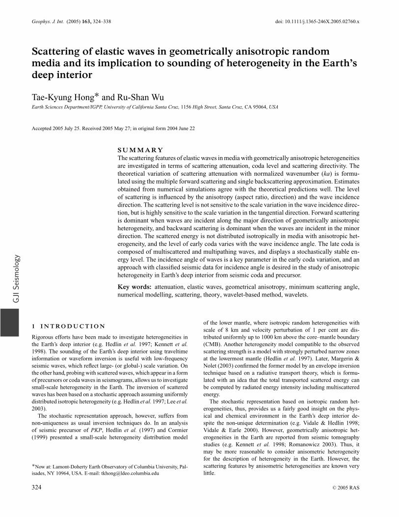
Figure 1. Synthetic P-wave record sections from geometrical anisotropicrandom media at various incidence angles (ϕ i = 0, 30, 45, 60, 90◦). The ani-sometric heterogeneity is horizontally elongated, and the scales are 4010 min the horizontal direction and 501 m in the vertical direction. The propa-gation distance is 49.1 km. The other physical properties of the medium aredescribed in Section 5. The waveforms in both primary and coda changedrastically with the incidence angle.

The scattering attenuation in anisometric random medium hasbeen investigated in a limited view previously, for instance, paraxialwave incidence on anisometric heterogeneous medium (Wagner &Langston 1992; Roth & Korn 1993). Recently, traveltime variation(Samuelides & Mukerji 1998; Iooss et al. 2000; Kravtsov et al.2003) and amplitude fluctuation (Muller & Shapiro 2003) in aniso-metric random media were investigated in terms of incidence angle.However, the influence of the incidence angle on scattering atten-uation remains still unclear, and the way to investigate anisometricheterogeneities has been rarely discussed.

In scattering by anisometric heterogeneity, the incidence angleto the heterogeneity looks an important factor. Because appar-ent scale of heterogeneity varies with the incidence direction. InFig. 1, synthetic record sections from anisometric random mediaare presented. The waveforms in both primary and coda changedrastically with the incidence angle. Thus, the investigation ofscattering features for change of incidence angle will help us tounderstand more clearly the physical composition in the Earth’sinterior. In particular, the core phases, PKP, display a specificincidence angle to the CMB with epicentral distance; for in-stance, PKPdf (PKIKP) shows a nearly vertical incidence to theCMB at distances around 180◦, and the incidence angle of thePKPbc branch varies from about 30◦ to 60◦ at distances around140◦.

In this study, we mainly focus on the investigation of scat-tering attenuation variation, coda and scattered energy transmis-sion in anisometric random media. For this purpose, we formu-late a theoretical scattering attenuation expression for anisomet-ric media. The theoretical expression is compared with the esti-mates from numerical simulations. Various sets of physical pa-rameters are considered for models, and the influence of eachparameter on scattering is investigated. In particular, the influ-ence of incidence angle on the scattering energy distribution andcoda level is discussed. Also, the difference in scattering be-tween anisometric and isotropic random media is examined. Fi-nally, we discuss the way to estimate correctly the physical propertyof anisometric heterogeneity in the Earth from observed seismicdata.

2 T H E O R E T I C A L E X P R E S S I O N O FS C AT T E R I N G AT T E N UAT I O N I NA N I S O M E T R I C R A N D O M M E D I A

Theoretical scattering attenuation expression for anisometric ran-dom media can be formulated by expanding the approach forisotropic random media (Hong & Kennett 2003a; Hong 2004). Notethat Wu & Aki (1985b) derived a general formulation of scatteringcoefficients, which can be applied to both isotropic and anisometricrandom media.

Here we consider the scattering of 2-D elastic waves. The 2-Delastic wave equations are given by

ρ0∂2u0

x

∂t2= ∂σ 0

xx

∂x+ ∂σ 0

xz

∂z, ρ0

∂2u0z

∂t2= ∂σ 0

zx

∂x+ ∂σ 0

zz

∂z, (1)

where

σ 0xx = (λ0 + 2µ0)

∂u0x

∂x+ λ0

∂u0z

∂z,

σ 0zz = λ0

∂u0x

∂x+ (λ0 + 2µ0)

∂u0z

∂z, (2)

σ 0xz = µ0

(∂u0

x

∂z+ ∂u0

z

∂x

)(3)

and λ0 and µ0 are the Lame coefficients, and ρ 0 is the density inthe background medium.

The perturbations in physical parameters (ρ = ρ 0 + δρ, λ =λ0 + δλ, µ = µ0 + δµ) cause wave scattering, and can be treatedas equivalent body forces ( f s

x , f sz ) for the scattered field:

ρ∂2u0

x

∂t2− ∂σxx

∂x− ∂σxz

∂z= f s

x , ρ∂2u0

z

∂t2− ∂σzx

∂x− ∂σzz

∂z= f s

z .

(4)

For vertically incident P waves (u0x = 0, us

z = exp[i(kαz − ωt)]), eq.(4) can be written by (Hong & Kennett 2003a)

f sx = −ikα

∂(δλ)

∂xu0

z ,

f sz = −

{k2

α

(α2

0δρ − δλ − 2δµ) + ikα

∂(δλ + 2δµ)

∂z

}u0

z .(5)

Here, the variations of physical parameters in the Earth are stronglycorrelated to each other (Birch 1961; Shiomi et al. 1997; Romanow-icz 2001), so the S-wave velocity perturbation and the density pertur-bation can be expressed in terms of the P-wave velocity perturbation(ξ ):

ξ (x, z) = ∂α

α0= 1

Kβ

δβ

β0= 1

Kρ

δρ

ρ0, (6)

where α0 is the P-wave velocity in the background medium, β 0

the S-wave velocity, and ρ 0 the density. K β and K ρ are constantsdetermining the relative strengths of S-velocity perturbation anddensity perturbation to the P-velocity perturbation.

Using the relationship in (6), the body forces in (5) can be ex-pressed in terms of ξ :

f sx = −ikαα

20ρ0C1

∂ξ

∂xexp[i(kαz − ωt)],

f sz =

(2k2

αα20ρ0ξ − ikαα

20ρ0C2

∂ξ

∂z

)exp[i(kαz − ωt)], (7)

where C 1 and C 2 are

C1 = (2 + Kρ) − 2

γ 2(2Kβ + Kρ), C2 = 2Kβ + Kρ (8)

C© 2005 RAS, GJI, 163, 324–338

326 T.-K. Hong and R.-S. Wu

and γ = α0/β 0. The remaining derivation procedure follows theprocedure in previous studies. A summarized derivation procedureof scattering attenuation is presented in Appendix A.

Finally, the theoretical scattering attenuation expression(Q−1/ε2), based on the multiple forward scattering and singlebackscattering approximation, is given by

Q−1s

ε2= k2

αWr

(4π )2

∫ 2π−θmin

θmin

P(k∗

r

)dθ

+ k2αγ

2Wt

(4π )2

∫ 2π−θmin−�φ

θmin+�φ

P(k∗

t

)dθ, (9)

where θ min is the minimum scattering angle, ε is the standard devi-ation of perturbation, P is the power spectral density function, and�φ is given by

�φ = φP − φS, φP = π − θmin

2, φS = sin−1

(sin φP

γ

). (10)

The wavenumber vector k∗j ( j = r , t) is given by

k∗r = kα(1 − cos θ, − sin θ ), k∗

t = kα(1 − γ cos θ, −γ sin θ ),(11)

and the coefficient Wj is

Wr = (64 + 7C2

1 − 64C2 + 28C22

)/32,

Wt = (64 − 64C2 + 16C2

2 + γ 2C21 + 4γ 2C2

2

)/32. (12)

Here, the coefficient Wj reflects the average coefficient strength forevery scattering angle. The eq. (9) is the general scattering attenu-ation solution for anisometric random medium, and can be applieddirectly if the PSDF is known. The PSDF for paraxial incidence sys-tem can be formulated easily, but the PSDF for inclined incidencesystem needs to be formulated with consideration of incidence an-gle. The discussion is expanded in Section 4.

3 A N I S O M E T R I C R A N D O M M E D I A

We follow the notation and the terminology used in the geostatis-tics (Deutsch & Journel 1998) for description of geometricallyanisotropic model. The direction of the largest correlation distanceis called the major direction, and the tangential direction, with thesmallest correlation distance, is referred as the minor direction. Theheterogeneity scales in the major and minor directions are used forthe construction of anisometric structure.

We first consider paraxial systems where the major direction isalong either of the coordinate axes. The anisometric random het-erogeneity can be modelled by extending the isotropic heterogene-ity expression. The 2-D exponential autocorrelation function (ACF,N (x)) of anisometric random heterogeneity and its power spectraldensity function (PSDF,P(k)) are given by (e.g. Iooss 1998)

N (x, z) = exp

[− r ′

a′

], P(kx , kz) = 2πVa{

1 + (k ′a′)2}3/2 , (13)

where ax and a z are the correlation distances (scales) of stochasticrandom heterogeneity in x- and z-axis directions, and kx and k z arethe wavenumbers along the axis directions. The r′/a′, k′ a′, and Va

in (13) are given by

r ′

a′ =√

x2

a2x

+ z2

a2z

, k ′a′ =√

k2x a2

x + k2z a2

z , Va = ax az . (14)

The ACF and PSDF of Gaussian random medium are

N (x, z) = exp

[−

(r ′

a′

)2]

, P(kx , kz) = πVa exp

[− (k ′a′)2

4

],

(15)

and the von Karman ACF and PSDF are

N (x, z) = 1

2ν−1�(ν)

(r ′

a′

)ν

Kν

(r ′

a′

),

P(kx , kz) = 4πνVa{1 + (k ′a′)2

}ν+1 , (16)

where ν is the Hurst number, � is the Gamma function, and K ν

is the modified Bessel function of order of ν. Here the exponentialrandom media correspond to von Karman media with Hurst numberof 0.5.

4 E X PA N S I O N T O I N C L I N E DA N I S O M E T R I C R A N D O M M E D I A

In anisometric random media, the stochastic heterogeneity scalesin the incident and tangential directions change with the wave inci-dence angle. Thus, it is expected that the scattering strength changeswith the incidence angle. This effect is observed in a form of az-imuthal anisotropy in field data analysis. As the wave front approach-ing to the deep Earth is nearly planar, the incident waves are welldefined with the incidence angle and the geometry of the anisomet-ric system can be represented with the relative incidence angle forthe anisometric heterogeneity.

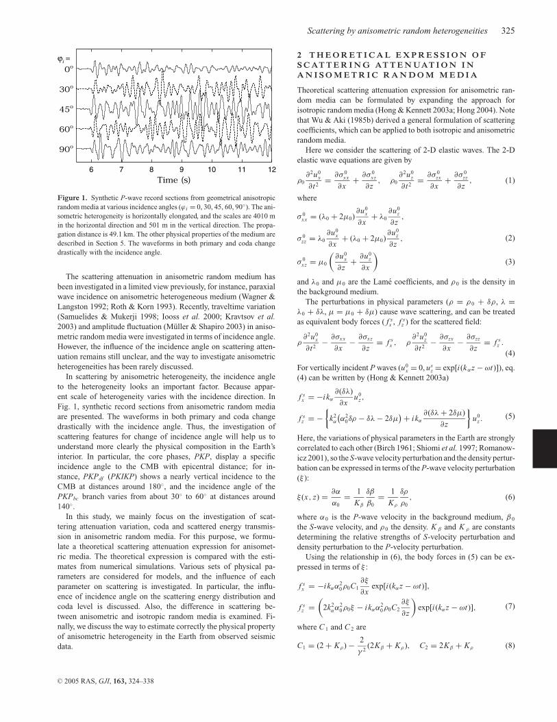
For convenience in numerical simulation and analysis, the in-cidence angle is considered in the system by rotating the ran-dom medium instead of considering inclined wave incidence (see,Fig. 2a). The implementation of rotated anisometric medium pro-vides several advantages over the consideration of inclined waveincidence. With application of periodic boundary condition at theleft and right artificial boundaries of medium, we can imitate a hor-izontally unbounded random medium. Also, the scattered energyexchanged across the artificial boundaries can be considered cor-rectly. Note that the incidence angle considered in this study is therelative angle between the wave incidence direction and the minordirection of heterogeneity. Thus, the results can be extended straight-forwardly to field observation by considering the relative incidenceangle.

We have presented the theoretical scattering attenuation expres-sion for paraxial system in (9), where waves are incident alongthe major or minor direction. The scattering attenuation in a ran-dom medium is the stochastic energy loss by scattering on hetero-geneities. The individual ray is interfered by perturbation along theray path, and the scattering of incident waves is dominantly influ-enced by the apparent scales of heterogeneity in the incident and thetangential direction. Thus, the heterogeneity in inclined incidencesystem can be represented with stochastic scales in the incident andtangential directions.

The stochastic scales of inclined heterogeneity can be esti-mated through an angular rotation of the coordinate system (e.g.Samuelides & Mukerji 1998; Iooss et al. 2000):

1

ah=

√cos2 ϕi

a2x

+ sin2 ϕi

a2z

,1

av

=√

sin2 ϕi

a2x

+ cos2 ϕi

a2z

, (17)

where ϕ i is the relative incidence angle and av is the stochasticscale in the wave incidence direction and ah is the scale in the tan-gential direction. The theoretical variation of scattering attenuation

C© 2005 RAS, GJI, 163, 324–338


plane waves

heterogeneity

x

z

x´

z´

ϕi

ϕi

0

4

8

12

16

20

z (k

m)

0 4 8 12 16 20x (km)

(a) (b)

Figure 2. (a) The relative incidence angle (ϕ i ) is defined as the angle between the incidence direction (z) and the minimum direction of anisotropy (z′). x ′-axisdirection corresponds to the maximum direction of anisotropy, and x-axis direction is orthogonal to the incidence direction. (b) The geometrical anisotropicrandom medium with ax = 4010 m, a z = 501 m and ϕ i = 30◦.

in inclined system can be estimated using the stochastic scales ofheterogeneity, that is, ah and av instead of ax and a z are applied tothe computation of the spectral density functions (PSDF) in (13),(15) and (16). The theoretical scattering attenuation expression isvalidated by comparing to numerical results in Section 6.

5 N U M E R I C A L M O D E L L I N G

We consider a plausible set of physical properties at the upper man-tle from the Earth model by Kennett et al. (1995). We set P-wavevelocity to be 8.325 km s−1, S-wave velocity 4.5 km s−1, and thedensity 3.4 g cm−3. The size of medium is 45 × 90 km and the do-main is represented by 256 × 512 grid points. The top and bottomartificial boundaries are treated with absorbing boundary condition,and the artificial boundaries on both sides are considered to haveperiodic boundary condition that imitates horizontally unboundedmedia.

Plane P waves are incident vertically, and the source time func-tion is the Ricker wavelet with dominant frequency of 4.5 Hz. 12receiver arrays are deployed perpendicularly to the incidence direc-tion at every 5.45 km from the source position along the incidencedirection. Each receiver array consists of 256 receivers and the in-terval between adjacent receivers in a receiver array is 175.8 m. Thepropagation distances to the shortest and the longest receiver arraysare 5.45 and 65.39 km.

We consider the exponential anisometric random model (13). Therandom models are constructed in the wavenumber domain by as-signing random phases to a spectral density function at each gridpoint (Hong & Kennett 2003a). The spectral random variation is con-verted to spatial random variation by Fourier transform. The inclinedanisometric random media are designed by rotating a reference ran-dom model (see, Fig. 2b). We consider 5 per cent perturbation inP-wave velocity. The shear velocity perturbation is set to be twicethe P velocity perturbation (i.e. K β = 2), which is plausible in themantle (see, Robertson & Woodhouse 1996; Romanowicz 2001).The density perturbation is much less resolvable from seismic data(Kennett 1998; Romanowicz 2001). Considering the general rela-tionship between velocity and density in the Earth (Birch 1961; Sato

& Fehler 1998), we apply 4 per cent perturbation in the density (i.e.K ρ = 0.8).

We consider the vertical scale of anisometric heterogeneity as theminor scale, and the horizontal scale as the major scale. We set thehorizontal scale to vary in the order of 2 from 501 m through 1003 mand 2005 m to 4010 m, and the vertical scale (a z) to be constant by501 m. The apparent stochastic scales in inclined incidence systemvary with the relative incidence angle (ϕ i ). When ϕ i is 90◦, thestochastic scale in the incidence direction (av) is equal to ax. Weconsider five relative incidence angles (ϕ i ) of 0, 30, 45, 60 and 90◦

in the modelling.A wavelet-based method (Hong & Kennett 2002a,b, 2003b, 2004)

is used for modelling of wave propagation in these random media.The wavelet-based method is based on the full wave equation, andthe spatial differentiations (∂ x , ∂ z) in the wave equation are appliedin the wavelet space using an operator projection technique. Thespatial differentiation in wavelet space allows us to have accurateresponses of both high- and low-frequency variation in medium.Hong & Kennett (2003a) pointed out that artificial attenuation canbe included in numerical simulation in random media due to fre-quent variation in physical properties when a low order of numericalmodelling technique is applied. Also, the wavelet-based method isnumerically stable even in highly perturbed media, and thus suitablefor modelling in random media.

6 S C AT T E R I N G AT T E N UAT I O N

Scattered waves are generated when waves encounter hetero-geneities. In isotropic random media, the radiation pattern of in-cident waves controls the scattering energy distribution around aheterogeneity (Wu & Aki 1985a). In anisometric random media,the relative incidence angle plays an additional important role in thescattered energy distribution. Thus, the scattering feature in aniso-metric random medium can be identified with the relative incidenceangle and the aspect ratio between the major and minor scales.

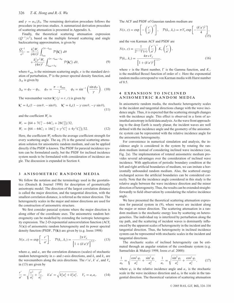
Fig. 3 displays synthetic time responses from anisometric ran-dom media with ax of 4010 m and a z of 501 m for various relativeincidence angles (ϕ i = 0, 30, 45, 60, 90◦). We present also the timeresponses from isotropic random medium (ax = a z = 4010 m) for

C© 2005 RAS, GJI, 163, 324–338


7

8

9

10

11

12

0 5 10 15 20 25 30 35 40 45Tim

e (s

)

Range (km)

Z

ϕi = 0o

7

8

9

10

11

12

0 5 10 15 20 25 30 35 40 45

Tim

e (s

)

Range (km)

Z

ϕi = 30o

7

8

9

10

11

12

0 5 10 15 20 25 30 35 40 45

Tim

e (s

)

Range (km)

Z

ϕi = 45o

7

8

9

10

11

12

0 5 10 15 20 25 30 35 40 45

Tim

e (s

)

Range (km)

Z

ϕi = 60o

7

8

9

10

11

12

0 5 10 15 20 25 30 35 40 45

Tim

e (s

)

Range (km)

Z

ϕi = 90o

7

8

9

10

11

12

0 5 10 15 20 25 30 35 40 45

Tim

e (s

)

Range (km)

Z

isotropic

(a) (b) (c)

(d) (e) (f)

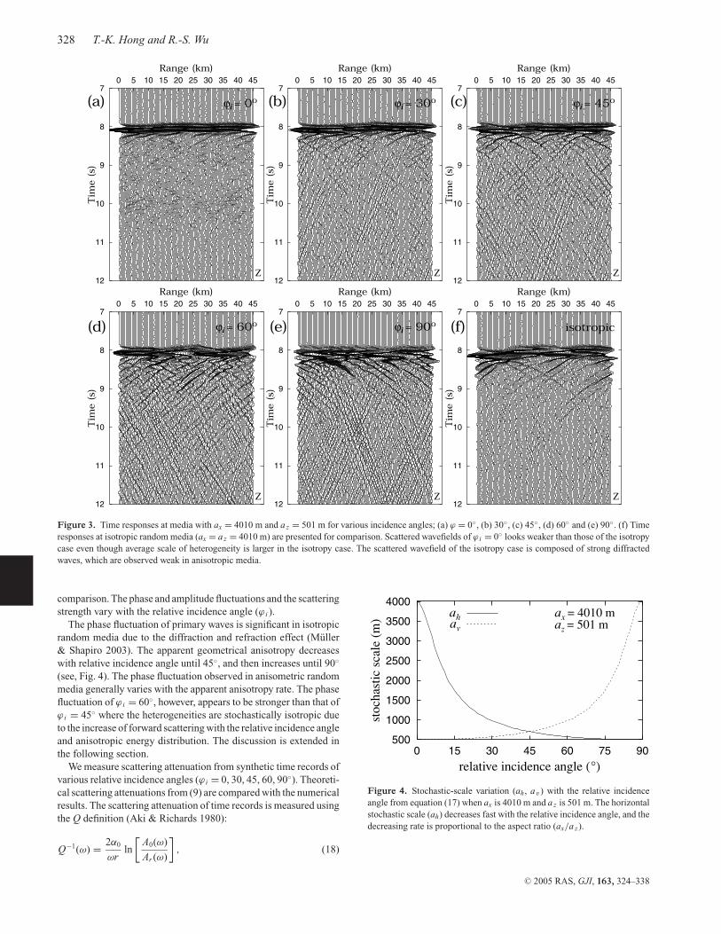
Figure 3. Time responses at media with ax = 4010 m and a z = 501 m for various incidence angles; (a) ϕ = 0◦, (b) 30◦, (c) 45◦, (d) 60◦ and (e) 90◦. (f) Timeresponses at isotropic random media (ax = a z = 4010 m) are presented for comparison. Scattered wavefields of ϕ i = 0◦ looks weaker than those of the isotropycase even though average scale of heterogeneity is larger in the isotropy case. The scattered wavefield of the isotropy case is composed of strong diffractedwaves, which are observed weak in anisotropic media.

comparison. The phase and amplitude fluctuations and the scatteringstrength vary with the relative incidence angle (ϕ i ).

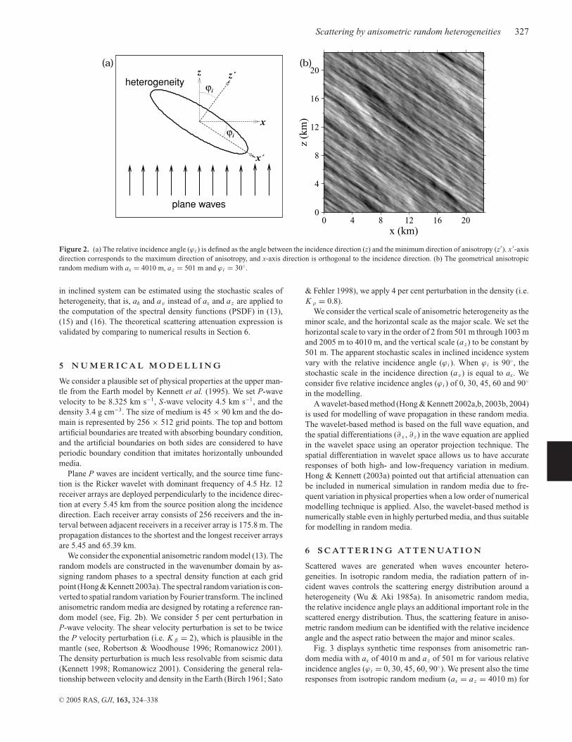
The phase fluctuation of primary waves is significant in isotropicrandom media due to the diffraction and refraction effect (Muller& Shapiro 2003). The apparent geometrical anisotropy decreaseswith relative incidence angle until 45◦, and then increases until 90◦

(see, Fig. 4). The phase fluctuation observed in anisometric randommedia generally varies with the apparent anisotropy rate. The phasefluctuation of ϕ i = 60◦, however, appears to be stronger than that ofϕ i = 45◦ where the heterogeneities are stochastically isotropic dueto the increase of forward scattering with the relative incidence angleand anisotropic energy distribution. The discussion is extended inthe following section.

We measure scattering attenuation from synthetic time records ofvarious relative incidence angles (ϕ i = 0, 30, 45, 60, 90◦). Theoreti-cal scattering attenuations from (9) are compared with the numericalresults. The scattering attenuation of time records is measured usingthe Q definition (Aki & Richards 1980):

Q−1(ω) = 2α0

ωrln

[A0(ω)

Ar (ω)

], (18)

500

1000

1500

2000

2500

3000

3500

4000

0 15 30 45 60 75 90

stoc

hast

ic s

cale

(m

)

relative incidence angle (°)

ax = 4010 maz = 501 m

ahav

Figure 4. Stochastic-scale variation (ah, av) with the relative incidenceangle from equation (17) when ax is 4010 m and a z is 501 m. The horizontalstochastic scale (ah) decreases fast with the relative incidence angle, and thedecreasing rate is proportional to the aspect ratio (ax/a z).

C© 2005 RAS, GJI, 163, 324–338


where ω is angular frequency, r is the propagation distance, and A0

and Ar are the spectral amplitudes at the origin and the receiver. Thespectral amplitudes of primary waves are measured by stacking theamplitudes of tapered records (Hong & Kennett 2003a, 2004).

Scattering attenuation is over or underestimated at short distance,and stable scattering attenuation can be measured at a sufficientlylarge distance (Hong et al. 2005). The seismograms of the 12threceiver array, the furthest array from the source position, are usedfor the scattering attenuation measurement. In Fig. 5, we compare the

0.01

0.1

1

0.1 1 10 100

QS-1

⁄ ε2

k ax

0o

30o

60o

90o

isotropic heterogeneity

isotropic

0.01

0.1

1

0.1 1 10 100Q

S-1 ⁄ ε

2k ax

0o

30o

60o

90o

0o

30o

60o90o

ϕi = 0o

isotropicanisotropic

0.01

0.1

1

0.1 1 10 100

QS-1

⁄ ε2

k ax

0o

30o

60o

90o

0o

30o

60o

90o

ϕi = 30o


0.01

0.1

1

0.1 1 10 100

QS-1

⁄ ε2

k ax

0o

30o

60o

90o

0o

30o

60o

90o

ϕi = 45o


0.01

0.1

1

0.1 1 10 100

QS-1

⁄ ε2

k ax

0o

30o

60o

90o

0o

30o

60o

90o

ϕi = 60o


0.01

0.1

1

0.1 1 10 100

QS-1

⁄ ε2

k ax

0o

30o

60o

90o

0o

30o

60o

90o ϕi = 90o


(a) (b)

(c) (d)

(e) (f)

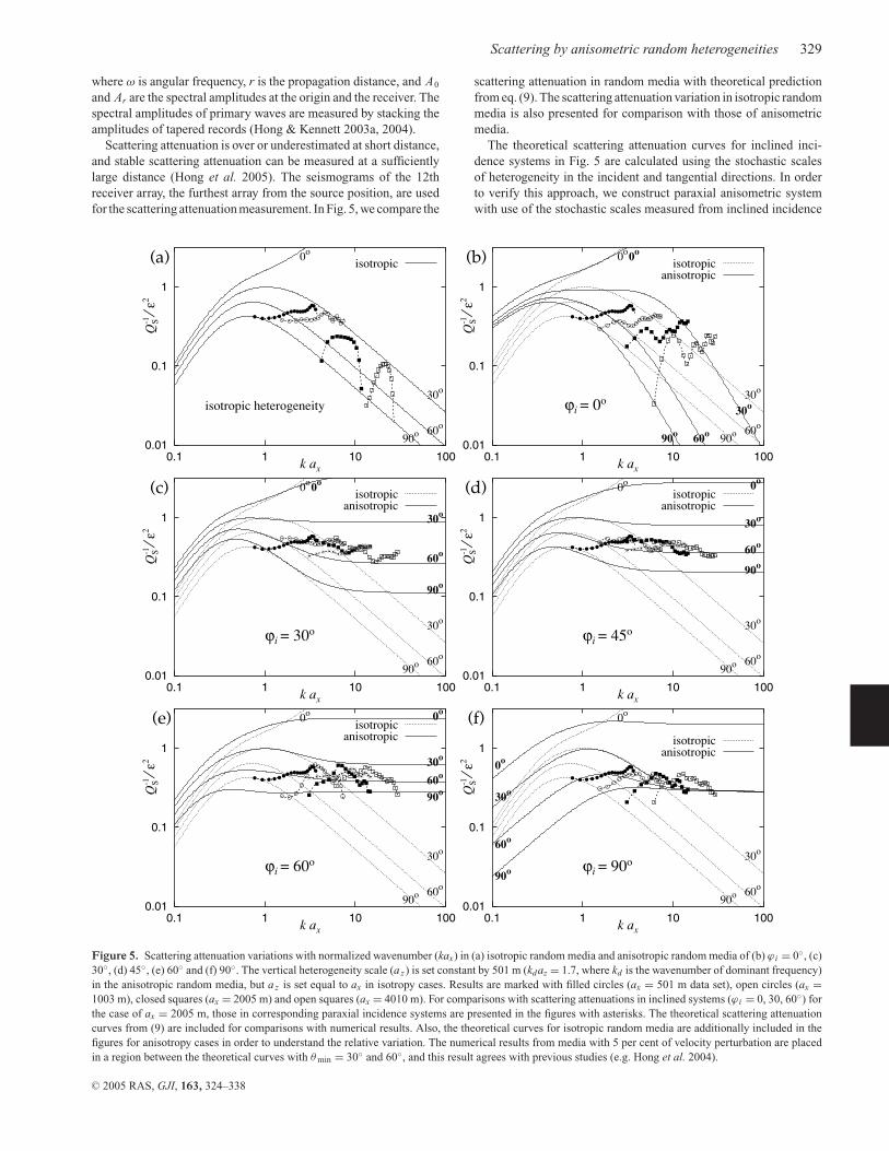
Figure 5. Scattering attenuation variations with normalized wavenumber (kax) in (a) isotropic random media and anisotropic random media of (b) ϕ i = 0◦, (c)30◦, (d) 45◦, (e) 60◦ and (f) 90◦. The vertical heterogeneity scale (a z) is set constant by 501 m (kdaz = 1.7, where kd is the wavenumber of dominant frequency)in the anisotropic random media, but a z is set equal to ax in isotropy cases. Results are marked with filled circles (ax = 501 m data set), open circles (ax =1003 m), closed squares (ax = 2005 m) and open squares (ax = 4010 m). For comparisons with scattering attenuations in inclined systems (ϕ i = 0, 30, 60◦) forthe case of ax = 2005 m, those in corresponding paraxial incidence systems are presented in the figures with asterisks. The theoretical scattering attenuationcurves from (9) are included for comparisons with numerical results. Also, the theoretical curves for isotropic random media are additionally included in thefigures for anisotropy cases in order to understand the relative variation. The numerical results from media with 5 per cent of velocity perturbation are placedin a region between the theoretical curves with θ min = 30◦ and 60◦, and this result agrees with previous studies (e.g. Hong et al. 2004).

scattering attenuation in random media with theoretical predictionfrom eq. (9). The scattering attenuation variation in isotropic randommedia is also presented for comparison with those of anisometricmedia.

The theoretical scattering attenuation curves for inclined inci-dence systems in Fig. 5 are calculated using the stochastic scalesof heterogeneity in the incident and tangential directions. In orderto verify this approach, we construct paraxial anisometric systemwith use of the stochastic scales measured from inclined incidence

C© 2005 RAS, GJI, 163, 324–338


systems, and calculate time records. The scattering attenuations ob-tained from inclined incidence systems and their equivalent paraxialincidence systems are compared for cases of ax = 2005 m and a z =501 m (see, Figs 5c–e). The scattering attenuations measured fromthe corresponding paraxial incidence systems are marked with as-terisks in the figures. The scattering attenuations between the twosystems are fairly close each other. This indicates that the scatteringattenuation in anisometric random media is dependent mainly onthe scales in the incident and tangential directions.

The measured scattering attenuations of all cases are placed in azone between the theoretical curves with minimum scattering angle(θ min) of 30◦ and 60◦. The minimum scattering angle is a stochasticangle span for correction of forward scattering energy that comple-ments the primary wave (Hong 2004). As the perturbation strengthin the medium increases, apparent coherent forward scattering isstrengthened at large normalized wavenumber (ka > 1) (Hong et al.2005). Thus, the minimum scattering angle appears to increase withperturbation strength at the large normalized wavenumber (Hong &Kennett 2003a; Hong et al. 2005).

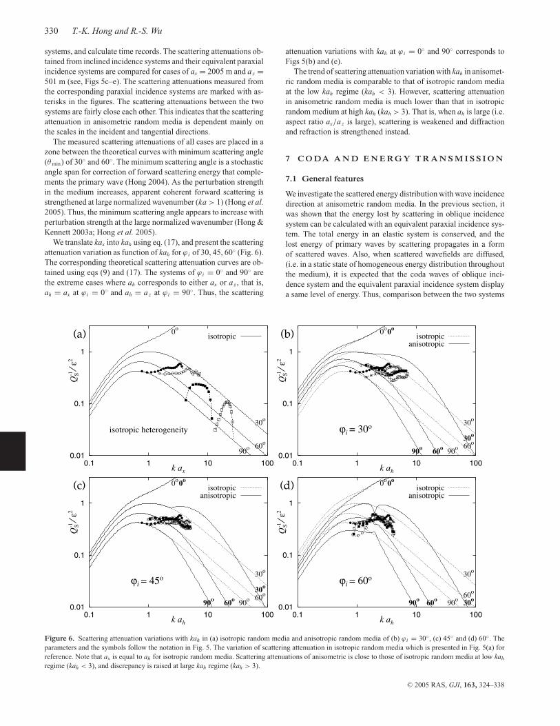
We translate kax into kah using eq. (17), and present the scatteringattenuation variation as function of kah for ϕ i of 30, 45, 60◦ (Fig. 6).The corresponding theoretical scattering attenuation curves are ob-tained using eqs (9) and (17). The systems of ϕ i = 0◦ and 90◦ arethe extreme cases where ah corresponds to either ax or a z , that is,ah = ax at ϕ i = 0◦ and ah = a z at ϕ i = 90◦. Thus, the scattering

0.01

0.1

1

0.1 1 10 100

QS-1

⁄ ε2

k ax

0o

30o

60o

90o

isotropic heterogeneity

isotropic

0.01

0.1

1

0.1 1 10 100

QS-1

⁄ ε2

k ah

0o

30o

60o

90o

0o

30o

60o90o

ϕi = 30o


0.01

0.1

1

0.1 1 10 100

QS-1

⁄ ε2

k ah

0o

30o

60o

90o

0o

30o

60o90o

ϕi = 45o


0.01

0.1

1

0.1 1 10 100

QS-1

⁄ ε2

k ah

0o

30o

60o

90o

0o

30o60o90o

ϕi = 60o


(a) (b)

(c) (d)

Figure 6. Scattering attenuation variations with kah in (a) isotropic random media and anisotropic random media of (b) ϕ i = 30◦, (c) 45◦ and (d) 60◦. Theparameters and the symbols follow the notation in Fig. 5. The variation of scattering attenuation in isotropic random media which is presented in Fig. 5(a) forreference. Note that ax is equal to ah for isotropic random media. Scattering attenuations of anisometric is close to those of isotropic random media at low kah

regime (kah < 3), and discrepancy is raised at large kah regime (kah > 3).

attenuation variations with kah at ϕ i = 0◦ and 90◦ corresponds toFigs 5(b) and (e).

The trend of scattering attenuation variation with kah in anisomet-ric random media is comparable to that of isotropic random mediaat the low kah regime (kah < 3). However, scattering attenuationin anisometric random media is much lower than that in isotropicrandom medium at high kah (kah > 3). That is, when ah is large (i.e.aspect ratio ax/a z is large), scattering is weakened and diffractionand refraction is strengthened instead.

7 C O DA A N D E N E RG Y T R A N S M I S S I O N

7.1 General features

We investigate the scattered energy distribution with wave incidencedirection at anisometric random media. In the previous section, itwas shown that the energy lost by scattering in oblique incidencesystem can be calculated with an equivalent paraxial incidence sys-tem. The total energy in an elastic system is conserved, and thelost energy of primary waves by scattering propagates in a formof scattered waves. Also, when scattered wavefields are diffused,(i.e. in a static state of homogeneous energy distribution throughoutthe medium), it is expected that the coda waves of oblique inci-dence system and the equivalent paraxial incidence system displaya same level of energy. Thus, comparison between the two systems

C© 2005 RAS, GJI, 163, 324–338


0.1

1

0 1 2 3 4 5 6 7 8 9 10 11

Am

plitu

de

Time (s)

ϕi = 45o

X, inclinedX, sto.-par.

0.1

1

0 1 2 3 4 5 6 7 8 9 10 11

Am

plitu

de

Time (s)

ϕi = 45o

Z, inclinedZ, sto.-par.

(a) (b)

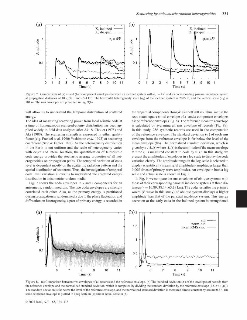
Figure 7. Comparisons of (a) x- and (b) z-component envelopes between an inclined system with ϕ i = 45◦ and its corresponding paraxial incidence systemat propagation distances of 10.9, 38.1 and 65.4 km. The horizontal heterogeneity scale (ax) of the inclined system is 2005 m, and the vertical scale (a z) is501 m. The rms envelopes are presented in Fig. 9(b).

will allow us to understand the temporal distribution of scatteredenergy.The idea of measuring scattering power from local seismic coda ata time of homogeneous scattered-energy distribution has been ap-plied widely in field data analyses after Aki & Chouet (1975) andAki (1980). The scattering strength is expressed in either qualityfactor (e.g. Frankel et al. 1990; Yoshimoto et al. 1993) or scatteringcoefficient (Sato & Fehler 1998). As the heterogeneity distributionin the Earth is not uniform and the scale of heterogeneity varieswith depth and lateral location, the quantification of teleseismiccoda energy provides the stochastic average properties of all het-erogeneities on propagation paths. The temporal variation of codalevel is dependent mostly on the scattering radiation pattern and thespatial distribution of scatterers. Thus, the investigation of temporalcoda level variation allows us to understand the scattered energydistribution in anisometric random media.

Fig. 7 shows the coda envelopes in x and z components for ananisometric random medium. The two coda envelopes are stronglycorrelated each other. Also, as the primary energy is partitionedduring propagation in random media due to the phase fluctuation anddiffraction on heterogeneity, a part of primary energy is recorded in

0.1

1

6 7 8 9 10 11

Am

plitu

de

Time (s)

0

0.5

1

1.5

2

6 7 8 9 10 11Time (s)

stdnorm. std

mean RMS env.

(a) (b)

Figure 8. (a) Comparison between rms envelopes of all records and the reference envelope. (b) The standard deviation (σ ) of the envelopes of records fromthe reference envelope and the normalized standard deviation, which is computed by dividing the standard deviation by the reference envelope (i.e. σ/A0(t)).The standard deviation is far below the level of the reference envelope, and the normalized standard deviation is measured almost constant by around 0.37. Thesame reference envelope is plotted in a log scale in (a) and in actual scale in (b).

the tangential component (Hong & Kennett 2003a). Thus, we use theroot-mean-square (rms) envelope of x- and z-component envelopesas the reference envelope (Fig. 8). The reference mean rms envelopeis calculated by averaging all rms envelope of records (Fig. 8a).In this study, 256 synthetic records are used in the computationof the reference envelope. The standard deviation (σ ) of each rmsenvelope from the reference envelope is far below the level of themean envelope (8b). The normalized standard deviation, which isgiven by σ/A0(t) where A0(t) is the amplitude of the mean envelopeat time t, is measured constant in coda by 0.37. In this study, wepresent the amplitudes of envelopes in a log scale to display the codavariation clearly. The amplitude range in the log scale is selected todisplay scientifically meaningful amplitudes (amplitudes larger than0.005 times of primary-wave amplitude). An envelope in both a logscale and actual scale is shown in Fig. 8.

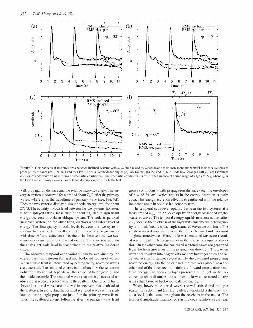
In Fig. 9, we compare the rms envelopes of oblique systems withthose of their corresponding paraxial incidence systems at three dis-tances (r = 10.89, 38.14, 65.39 km). The coda just after the primarywaves (P wave in this study) of oblique system displays a higheramplitude than that of the paraxial incidence system. This energyaccretion at the early coda in the inclined system is strengthened

C© 2005 RAS, GJI, 163, 324–338


0.1

1

0 1 2 3 4 5 6 7 8 9 10 11

Am

plitu

de

Time (s)

ϕi = 30o

RMS, inclinedRMS, sto.-par.

0.1

1

0 1 2 3 4 5 6 7 8 9 10 11

Am

plitu

de

Time (s)

ϕi = 45o


0.1

1

0 1 2 3 4 5 6 7 8 9 10 11

Am

plitu

de

Time (s)

ϕi = 60o


0.1

1

0 1 2 3 4 5 6 7 8 9 10 11

Am

plitu

de

Time (s)

ϕi = 60o

Tp

Tp

Tp /3

Tp 2Tp4Tp /3


(a) (b)

(c) (d)

Figure 9. Comparisons of rms envelopes between inclined systems with ax = 2005 m and a z = 501 m and their corresponding paraxial incidence systems atpropagation distances of 10.9, 38.1 and 65.4 km. The relative incidence angles (ϕ i ) are (a) 30◦, (b) 45◦ and (c) 60◦. Coda level changes with ϕ i . (d) Empiricaldivision of coda wave trains in terms of stochastic equilibrium. The stochastic equilibrium is established in coda at a time range of 4Tp/3 to 2Tp, where Tp isthe traveltime of primary waves. For detailed description, we refer to the text.

with propagation distance and the relative incidence angle. The en-ergy accretion is observed for a time of about Tp/3 after the primarywaves, where Tp is the traveltime of primary wave (see, Fig. 9d).Then the two systems display a similar coda energy level for about2Tp/3. The equality in coda level between the two systems, however,is not displayed after a lapse time of about 2Tp due to significantenergy decrease at coda in oblique system. The coda in paraxialincidence system, on the other hand, displays a consistent level ofenergy. The discrepancy in coda levels between the two systemsappears to increase temporally, and then decreases progressivelywith time. After a sufficient time, the codas between the two sys-tems display an equivalent level of energy. The time required forthe equivalent coda level is proportional to the relative incidenceangle.

The observed temporal coda variation can be explained by theenergy partition between forward and backward scattered waves.When a wave front is interrupted by heterogeneity, scattered wavesare generated. The scattered energy is distributed by the scatteringradiation pattern that depends on the shape of heterogeneity andthe incidence angle. The scattered waves propagating backward areobserved in receivers placed behind the scatterer. On the other hand,forward scattered waves are observed in receivers placed ahead ofthe scatterer. In particular, the forward scattered waves with a shal-low scattering angle propagate just after the primary wave front.Thus, the scattered energy following after the primary wave front

grows continuously with propagation distance (see, the envelopesof r = 65.39 km), which results in the energy accretion at earlycoda. This energy accretion effect is strengthened with the relativeincidence angle in oblique incidence system.

The temporal coda level equality between the two systems at alapse time of 4Tp/3 to 2Tp develops by an energy balance of single-scattered waves. The temporal energy equilibrium dose not last after2 Tp because the thickness of the layer with anisometric heterogene-ity is limited. In early coda, single scattered waves are dominant. Thesingle scattered waves in coda are the sum of forward and backwardsingle scattered waves. Here, the forward scattered waves are a resultof scattering at the heterogeneities in the reverse propagation direc-tion. On the other hand, the backward scattered waves are generatedfrom the heterogeneities in the propagation direction. Thus, whenwaves are incident into a layer with random heterogeneities, the re-ceivers at short distances record mainly the backward-propagatingscattered energy. On the other hand, the receivers placed near theother end of the layer record mainly the forward-propagating scat-tered energy. The coda envelopes presented in eq. (9) are for re-ceivers at short distances, the sources of forward scattered energyis less than those of backward scattered energy.

When, however, scattered waves are well mixed and multiplescattering is dominant (i.e. the scattered wavefield is diffused), thecoda level is the same throughout the receivers in the media. Thetemporal amplitude variation of seismic coda satisfies a rule (e.g.

C© 2005 RAS, GJI, 163, 324–338


Sato & Fehler 1998):

A(t) = C1

t pexp

[− ωt

2Qc

], (19)

where ω is the angular frequency, t is time, C is a constant, Qc isthe coda quality factor, p is the geometrical spreading parameterwith a value 1.0 for 3-D body waves, and 0.5 for 2-D body waves(equivalently, 3-D surface waves). When the coda is diffused, it isdominantly influenced by the intrinsic attenuation (Q−1

i ) that countsfor the inelastic absorption in the media, that is, Qc ≈Qi (Shapiroet al. 2000). Thus, the temporal coda variation can be expressed

0.1

1

2 3 4 5 6 7 8 9 10 11

Am

plitu

de

Time (s)

ϕi = 0o

RMS, 1a0RMS, 2a0RMS, 4a0RMS, 8a0

0.1

1

2 3 4 5 6 7 8 9 10 11A

mpl

itude

Time (s)

ϕi = 30o


0.1

1

2 3 4 5 6 7 8 9 10 11

Am

plitu

de

Time (s)

ϕi = 45o


0.1

1

2 3 4 5 6 7 8 9 10 11

Am

plitu

de

Time (s)

ϕi = 60o


0.1

1

2 3 4 5 6 7 8 9 10 11

Am

plitu

de

Time (s)

ϕi = 90o


0.1

1

2 3 4 5 6 7 8 9 10 11

Am

plitu

de

Time (s)

A(t) = C t-0.5

isotropic


(a) (b)

(c) (d)

(e) (f)

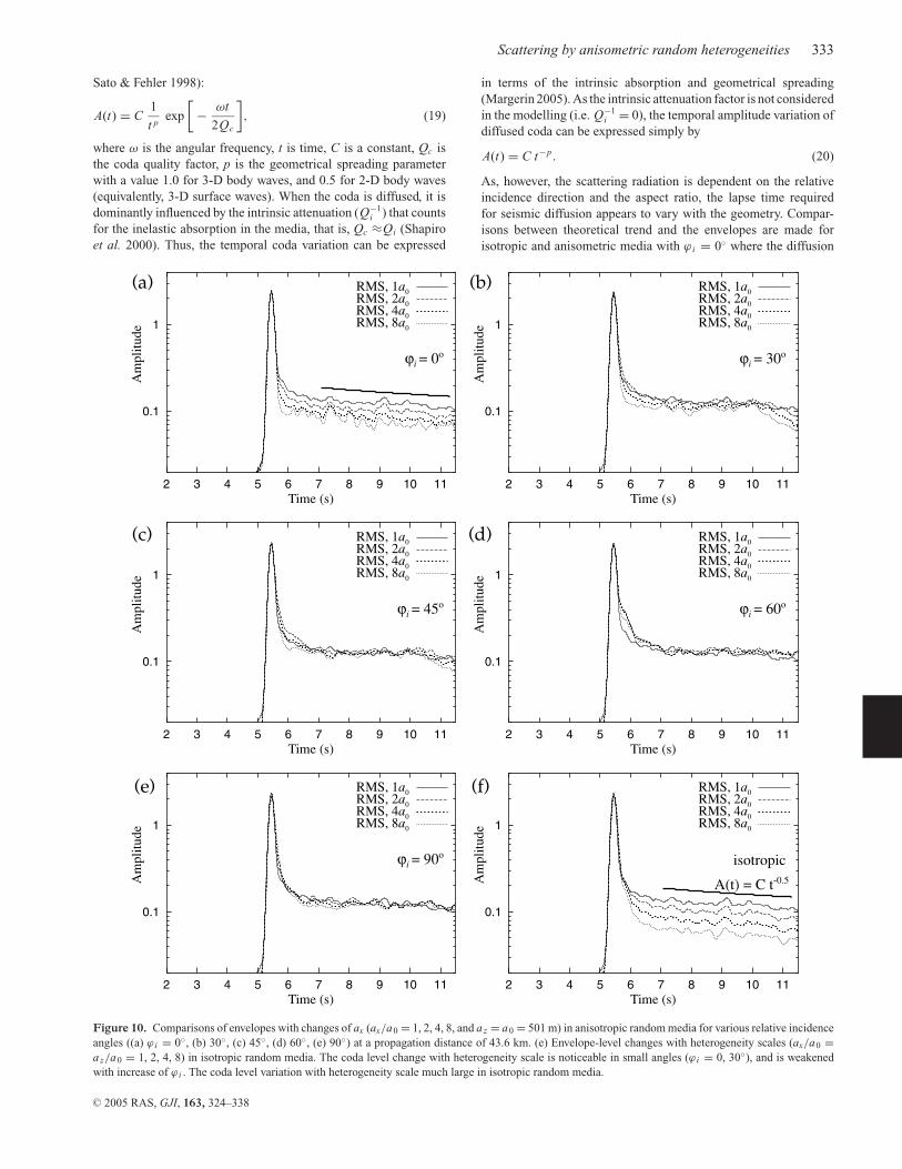
Figure 10. Comparisons of envelopes with changes of ax (ax/a0 = 1, 2, 4, 8, and a z = a0 = 501 m) in anisotropic random media for various relative incidenceangles ((a) ϕ i = 0◦, (b) 30◦, (c) 45◦, (d) 60◦, (e) 90◦) at a propagation distance of 43.6 km. (e) Envelope-level changes with heterogeneity scales (ax/a0 =a z/a0 = 1, 2, 4, 8) in isotropic random media. The coda level change with heterogeneity scale is noticeable in small angles (ϕ i = 0, 30◦), and is weakenedwith increase of ϕ i . The coda level variation with heterogeneity scale much large in isotropic random media.

in terms of the intrinsic absorption and geometrical spreading(Margerin 2005). As the intrinsic attenuation factor is not consideredin the modelling (i.e. Q−1

i = 0), the temporal amplitude variation ofdiffused coda can be expressed simply by

A(t) = C t−p. (20)

As, however, the scattering radiation is dependent on the relativeincidence direction and the aspect ratio, the lapse time requiredfor seismic diffusion appears to vary with the geometry. Compar-isons between theoretical trend and the envelopes are made forisotropic and anisometric media with ϕ i = 0◦ where the diffusion

C© 2005 RAS, GJI, 163, 324–338


0.1

1

2 3 4 5 6 7 8 9 10 11

Am

plitu

de

Time (s)

ratio = 2

RMS, 0o

RMS, 30o

RMS, 45o

RMS, 60o

RMS, 90o

0.1

1

2 3 4 5 6 7 8 9 10 11

Am

plitu

de

Time (s)

ratio = 4

RMS, 0o

RMS, 30o

RMS, 45o

RMS, 60o

RMS, 90o

0.1

1

2 3 4 5 6 7 8 9 10 11

Am

plitu

de

Time (s)

ratio = 8

RMS, 0o

RMS, 30o

RMS, 45o

RMS, 60o

RMS, 90o

(a)

(b)

(c)

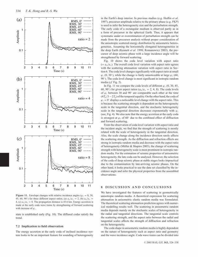
Figure 11. Envelope changes with relative incidence angles (ϕ i = 0, 30,45, 60, 90◦) for three different aspect ratios; (a) ax/a z = 2, (b) ax/a z =4, (c) ax/a z = 8. The propagation distance is 43.6 km. Energy accretion ismade at the early coda wave trains by strengthening of forward scatteringwith increase of ϕ i .

state is established early (Fig. 10). The diffused codas satisfy thetrend.

7.2 Implication to field observation

The energy accretion at the early coda of inclined incidence sys-tem looks to be an important feature for sounding of heterogeneity

in the Earth’s deep interior. In previous studies (e.g. Hedlin et al.1997), precursor amplitude relative to the primary phase (e.g. PKP)is used to infer the heterogeneity size and the perturbation strength.The early coda of a rectangular medium is observed partly as ina form of precursor in the spherical Earth. Thus, it appears thatsystematic under or overestimation of perturbation strength can bemade from the precursor analysis without proper consideration ofthe anisotropic scattered energy distribution by anisometric hetero-geneities. Assuming the horizontally elongated heterogeneities inthe deep Earth (Kennett et al. 1998; Romanowicz 2003), the pre-cursor of deep seismic phase with a large incidence angle will bestrengthened by forward scattering.

Fig. 10 shows the coda level variation with aspect ratio(= ax/a z). The overall coda level variation with aspect ratio agreeswith the scattering attenuation variation with aspect ratio in Sec-tion 6. The coda level changes significantly with aspect ratio at smallϕ i (0, 30◦), while the change is fairly unnoticeable at large ϕ i (60,90◦). The coda level change is most significant in isotropic randommedia (cf. Fig. 5).

In Fig. 11 we compare the coda levels of different ϕ i (0, 30, 45,60, 90◦) for given aspect ratios (ah/av = 2, 4, 8). The coda levelsof ϕ i between 30 and 90◦ are comparable each other at the time(4Tp/3−2Tp) of the temporal equality. On the other hand, the coda ofϕ i = 0◦ displays a noticeable level change with the aspect ratio. Thisis because the scattering strength is dependent on the heterogeneityscale in the tangential direction, and the stochastic heterogeneityscale in the tangential direction decreases exponentially with ϕ i

(see, Fig. 4). We also note that the energy accretion at the early codais strongest at ϕ i of 60◦ due to the combined effect of diffractionand forward scattering.

From the observation of coda level variation with aspect ratio andthe incident angle, we find that the strength of scattering is mostlyrelated with the scale of heterogeneity in the tangential direction.Also, the scale change along the incidence direction rarely affectsthe scattering strength. As the diffraction and refraction effects arestrong in isotropic random media and decrease with the aspect ratioof heterogeneity (Muller & Shapiro 2003), the change of scatteringstrength with heterogeneity scale is most prominent in isotropic ran-dom media. For the estimation of seismic properties of anisometricheterogeneity, the late coda can be analysed. However, the selectionof the coda of deep seismic phase at stable stages looks impracticaldue to the contamination by late-arriving seismic phases. On theother hand, it looks practical to use the data set classified by the in-cidence angle and infer the physical properties from the assembledobservations.

8 D I S C U S S I O N A N D C O N C L U S I O N S

We have investigated the features of scattering in geometricallyanisotropic random media. A theoretical expression for scatteringattenuation in anisometric elastic random media was formulated.The theoretical scattering attenuation prediction agrees with numer-ical modelling results well. The scattering in anisometric randommedia depends mainly on the stochastic scales of heterogeneity inthe radial and tangential directions. The tangential scale controlsthe scattering strength, and the aspect ratio between the radial andtangential scales affects the strength of diffraction and refractionon the heterogeneity.

The coda shape in anisometric random media is highly dependenton the nature of heterogeneity such as aspect ratio and geometryand the wave incidence angle. Coda wave trains can be divided into

C© 2005 RAS, GJI, 163, 324–338


several parts following the constituting scattered energy composi-tion. Forward scattering is strengthened with the relative incidenceangle, and the forward scattered waves enhance the early coda. Theenergy accretion by the forward scattered waves increases with thepropagation distance and the relative incidence angle. This effect isexpected to enhance the precursor and early coda of deep seismicphase travelling through anisometric heterogeneous media.

Scattering level varies sensitively to the tangential scale of het-erogeneity. Thus, it appears that the sounding of anisometric hetero-geneity in the Earth’s deep interior from precursors or coda shouldbe operated by taking account of the incidence direction of the pri-mary phase. To this end it may be a way to examine the coda levelvariation from seismic data set that is classified by the incidenceangle of primary wave. This approach would be particularly usefulfor deep seismic phases due to their plane wave fronts.

Velocity anisotropy and intrinsic attenuation would be additionalfactors to be considered for conceivable investigation of heterogene-ity in the Earth. However, the strength of velocity anisotropy (e.g.Panning & Romanowicz 2004) is usually trivial compared to the ve-locity and density perturbation strength. Also, since coda attenuationis the sum of scattering and intrinsic attenuation and the intrinsicattenuation variation is correlated with the scattering attenuationvariation, the general scattering feature by anisometric heterogene-ity observed in the coda variation is expected to be preserved.

We have considered geometrical anisotropy with an idea that theheterogeneity in the Earth can be represented in terms of continu-ous stochastic random heterogeneities. However, a localized hetero-geneity region composed of discrete anisometric scatterers is alsoexpected in the Earth, for instance partial melting region (Vidale &Hedlin 1998). The investigation of scattering by discrete anisometricheterogeneities may be required in this direction.

A C K N O W L E D G M E N T S

TKH is grateful to Prof Brian Kennett for the discussion on deepseismic phases and coda waves and for allowing him to access tothe Supercomputer Facility in Australian National University, whichis also acknowledged for allocation of computational time. We aregrateful to the comments of Prof Rob van der Hilst and two anony-mous reviewers, which improved the paper. The research is sup-ported by a grant from DOE/BES at University of California, SantaCruz.

R E F E R E N C E S

Aki, K., 1980. Attenuation of shear waves in the lithosphere for frequenciesfrom 0.05 to 25 Hz, Phys. Earth planet. Inter., 21, 50–60.

Aki, K. & Chouet, B., 1975. Origin of coda waves: source, attenuation, andscattering effects, J. geophys. Res., 80, 3322–3342.

Aki, K. & Richards, P.G., 1980. Quantitative Seismology: Theory andMethods, Vol. 1, W.H. Freeman and Company, San Francisco.

Birch, F., 1961. The velocity of compressional waves in rocks to 10 kilobars,Part 2, J. geophys. Res., 66, 2199–2224.

Burridge, R., 1976. Some Mathematical Topics in Seismology, CourantInstitute of Mathematical Sciences, New York University, New York.

Cormier, V.F., 1999. Anisotropy of heterogeneity scale lengths in the lowermantle from PKIKP precursors, Geophys. J. Int., 136, 373–384.

Deutsch, C.Y. & Journel, A.G., 1998. GSLIB: Geostatistical SoftwareLibrary and User’s Guide, 2nd edn, Oxford University Press, New York.

Frankel, A., McGarr, A., Bicknell, J., Mori, J., Seeber, L. & Cranswick,E., 1990. Attenuation of high-frequency shear waves in the crust, mea-surements from New York State, South Africa, and southern California,J. geophys. Res., 95, 17 441–17 457.

Hedlin, M.A.H., Shearer, P.M. & Earle, P.S., 1997. Seismic evidence forsmall-scale heterogeneity throughout the Earth’s mantle, Nature, 387,145–150.

Hong, T.-K., 2004. Scattering attenuation ratios of P and S waves in elasticmedia, Geophys. J. Int., 158, 211–224.

Hong, T.-K. & Kennett, B.L.N., 2002a. A wavelet-based method for simula-tion of two-dimensional elastic wave propagation, Geophys. J. Int., 150,610–638.

Hong, T.-K. & Kennett, B.L.N., 2002b. On a wavelet-based method for thenumerical simulation of wave propagation, J. Comput. Phys., 183, 577–622.

Hong, T.-K. & Kennett, B.L.N., 2003a. Scattering attenuation of 2-D elasticwaves: theory and numerical modelling using a wavelet-based method,Bull. seism. Soc. Am., 93, 922–938.

Hong, T.-K. & Kennett, B.L.N., 2003b. Modelling of seismic waves in het-erogeneous media using a wavelet-based method: application to fault andsubduction zones, Geophys. J. Int., 154, 483–498.

Hong, T.-K. & Kennett, B.L.N., 2004. Scattering of elastic waves in mediawith a random distribution of fluid-filled cavities: theory and numericalmodelling, Geophys. J. Int., 159, 961–977.

Hong, T.-K., Kennett, B.L.N., Wu, R.-S., 2004. Effects of the den-sity perturbation in scattering, Geophys. Res. Lett., 31 (13), L13602,doi:10.1029/2004GL019933.

Hong, T.-K., Wu, R.-S. & Kennett, B.L.N., 2005. Stochastic features ofscattering, Phys. Earth planet. Inter., 148, 131–148.

Iooss, B., 1998. Seismic reflection traveltimes in two-dimensional statisti-cally anisotropic random media, Geophys. J. Int., 135, 999–1010.

Iooss, B., Blanc-Benon, P. & Lhuillier, C., 2000. Statistical moments of traveltimes at second order in isotropic and anisotropic random media, WavesRandom Media, 10, 381–394.

Kennett, B.L.N., 1998. On the density distribution within the Earth, Geophys.J. Int., 132, 374–382.

Kennett, B.L.N., Engdahl, E.R. & Buland, R., 1995. Constraints on seis-mic velocities in the earth from travel times, Geophys. J. Int., 122,108–124.

Kennett, B.L.N., Widiyantoro, S. & van der Hilst, R.D., 1998. Joint seismictomography for bulk sound and shear wave speed in the Earth’s mantle,J. geophys. Res., 103, 12 469–12 493.

Kravtsov, Y.A., Muller, T.M., Shapiro, S.A. & Buske, S., 2003. Statisticalproperties of reflection traveltimes in 3-D randomly inhomogeneous andanisometric media, Geophys. J. Int., 154, 841–851.

Lee, W.S., Sato, H. & Lee, K., 2003. Estimation of S-wave scatteringcoefficient in the mantle from envelope characteristics before and af-ter the ScS arrival, Geophys. Res. Lett., 30 (24), 2248, doi:10.1029/2003GL018413.

Margerin, L., 2005. Introduction to radiative transfer of seismic waves, inSeismic data analysis with global and local arrays, eds Levander, A. &Nolet, G., AGU Monograph Series, (in press).

Margerin, L. & Nolet, G., 2003. Multiple scattering of high-frequencyseismic waves in the deep Earth: PKP precursor analysis and in-version for mantle granularity, J. geophys. Res., 108(B11), 2514,doi:10.1029/2003JB002455.

Muller, T.M. & Shapiro, S.A., 2003. Amplitude fluctuations due to diffrac-tion and reflection in anisotropic random media: implications for seismicscattering attenuation estimates, Geophys. J. Int., 155, 139–148.

Panning, M. & Romanowicz, B., 2004. Inference on flow at the base ofEarth’s mantle based on seismic anisotropy, Science, 303, 351–353.

Robertson, G.S. & Woodhouse, J.H., 1996. Ratio of relative S to P velocityheterogeneity in the lower mantle, J. geophys. Res., 101(B9), 20 041–20 052.

Romanowicz, B., 2001. Can we resolve 3D density heterogeneity in the lowermantle?, Geophys. Res. Lett., 28, 1107–1110.

Romanowicz, B., 2003. 3D structure of the Earth’s lower mantle, C.R.Geoscience, 335, 23–35.

Roth, M. & Korn, M., 1993. Single scattering theory versus numerical mod-elling in 2-D random media, Geophys. J. Int., 112, 124–140.

Samuelides, Y. & Mukerji, T., 1998. Velocity shift heterogeneous media withanisotropic spatial correlation, Geophys. J. Int., 134, 778–786.

C© 2005 RAS, GJI, 163, 324–338


Sato, H. & Fehler, M., 1998. Seismic Wave Propagation and Scattering inthe Heterogeneous Earth, Springer-Verlag New York, Inc.

Shapiro, N.M., Campillo, M., Margerin, L., Singh, S.K., Kostoglodov, V. &Pacheco, J., 2000. The energy partitioning and the diffusive character ofthe seismic coda. Bull. seism. Soc. Am., 90, 655–665.

Shiomi, K., Sato, H. & Ohtake, M., 1997. Broadband power-bin spectra ofwell-log data in Japan, Geophys. J. Int., 120, 57–64.

Vidale, J.E. & Hedlin, M.A.H., 1998. Evidence for partial melt at the core-mantle boundary north of Tonga from the strong scattering of seismicwaves, Nature, 391, 682–685.

Vidale, J.E. & Earle, P.S., 2000. Fine-scale heterogeneity in the Earth’s innercore, Nature, 404, 273–275.

Wagner, G.S. & Langston, C.A., 1992. A numerical investigation of scat-tering effects for teleseismic plane wave propagation in a heteroge-neous layer over a homogeneous half-space, Geophys. J. Int., 110,486–500.

Wu, R.-S. & Aki, K., 1985a. Scattering characteristics of elastic waves byan elastic heterogeneity, Geophysics, 50, 582–595.

Wu, R.-S. & Aki, K., 1985b. Elastic wave scattering by a random mediumand the small-scale inhomogeneities in the lithosphere, J. geophys. Res.,90(B12), 10 261–10 273.

Yoshimoto, K., Sato, H. & Ohtake, M., 1993. Frequency-dependent atten-uation of P and S waves in the Kanto area, Japan, based on the coda-normalization method, Geophys. J. Int., 114, 165–174.

A P P E N D I X A : T H E O R E T I C A L D E R I VAT I O N O F S C AT T E R I N G AT T E N UAT I O NE X P R E S S I O N

We derive theoretical scattering attenuation expression for anisometric random media, based on the multiple forward scattering and singlebackscattering approximation (Hong & Kennett 2003a; Hong 2004). We omit the subscript 0 of symbols for the background properties tosimplify mathematical expressions.

Using the scattering forces ( f sj , j = x , z) in (5) and the Green’s function (Gjk , j , k = x , z) for 2-D elastic waves (Burridge 1976, p. 115),

we can express scattered wavefield (usj , j = x , z or 1,2) at position x by the perturbation at x′ as

usj (x) =

2∑k=1

∫S

f sk (x′)G jk(x, x′) dS(x′), (A1)

where S is the area of heterogeneity. The total scattered wavefield is composed of scattered P and S wavefields (uPPr , uPS

t ), and they can bewritten by (Hong & Kennett 2003a)

u P Pr (x) = sin θ u P P

x (x) + cos θ u P Pz (x)

= i

√kα

8π |x|Cr (θ ) exp

[− i

(ωt − kα|x| + π

4

)] ∫S

ξ (x′) exp[ikα(z − n · x′)] dS(x′),

u P St (x) = cos θ u P S

x (x) − sin θ u P Sz (x)

= i

√k3

αγ3

8π |x|Ct (θ ) exp

[− i

(ωt − kβ |x| + π

4

)] ∫S

ξ (x′) exp[ikα(z − γ n · x′)] dS(x′), (A2)

where Cr(θ ) and Ct(θ ) are

Cr (θ ) = sin θ{

C1 AP11(θ ) sin θ + 2AP

12(θ ) + C2 AP12(θ )(cos θ − 1)

}+ cos θ

{C1 AP

21(θ ) sin θ + 2AP22(θ ) + C2 AP

22(θ )(cos θ − 1)},

Ct (θ ) = cos θ{

C1 AS11(θ )γ sin θ + 2AS

12(θ ) + C2 AS12(θ )(γ cos θ − 1)

}− sin θ

{C1 AS

21(θ )γ sin θ + 2AS22(θ ) + C2 AS

22(θ )(γ cos θ − 1)}, (A3)

and Akij (i , j = 1,2, k = P, S) is

AP11(θ ) = sin2 θ, AP

12(θ ) = sin θ cos θ, AP21(θ ) = − sin θ cos θ, AP

22(θ ) = cos2 θ,

AS11(θ ) = cos2 θ, AS

12(θ ) = − sin θ cos θ, AS21(θ ) = sin θ cos θ, AS

22(θ ) = sin2 θ. (A4)

Here, θ is the scattering direction measured from the vertical axis (z, the incidence direction), and n is the unit vector in x direction.In order to estimate the total scattered energy, we calculate ensemble-averaged spectral power density of scattered waves:

⟨∣∣u P Pr

∣∣2⟩ = k3αWr

8π |x|×

∫S

∫S

〈ξ (x′)ξ (y′)〉 exp[ikα{ez · (x′ − y′) − n · (x′ − y′)}] dS(x′) dS(y′),

⟨∣∣u P St

∣∣2⟩ = k3αγ

3Wt

8π |x|×

∫S

∫S

〈ξ (x′)ξ (y′)〉 exp[ikα{ez · (x′ − y′) − γ n · (x′ − y′)}] dS(x′) dS(y′), (A5)

C© 2005 RAS, GJI, 163, 324–338


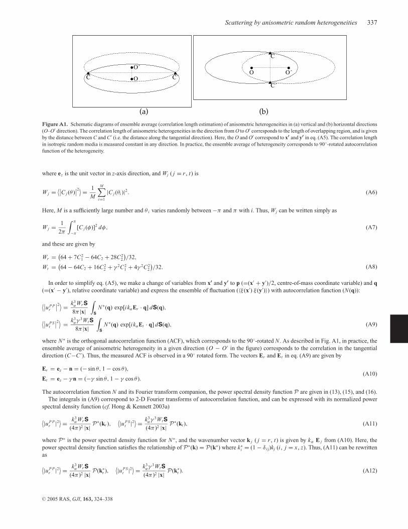
Figure A1. Schematic diagrams of ensemble average (correlation length estimation) of anisometric heterogeneities in (a) vertical and (b) horizontal directions(O–O′ direction). The correlation length of anisometric heterogeneities in the direction from O to O′ corresponds to the length of overlapping region, and is givenby the distance between C and C′ (i.e. the distance along the tangential direction). Here, the O and O′ correspond to x′ and y′ in eq. (A5). The correlation lengthin isotropic random media is measured constant in any direction. In practice, the ensemble average of heterogeneity corresponds to 90◦-rotated autocorrelationfunction of the heterogeneity.

where ez is the unit vector in z-axis direction, and Wj ( j = r , t) is

W j = ⟨∣∣C j (θ )∣∣2⟩ = 1

M

M∑i=1

|C j (θi )|2. (A6)

Here, M is a sufficiently large number and θ i varies randomly between −π and π with i. Thus, Wj can be written simply as

W j = 1

2π

∫ π

−π

[C j (φ)]2 dφ, (A7)

and these are given by

Wr = (64 + 7C2

1 − 64C2 + 28C22

)/32,

Wt = (64 − 64C2 + 16C2

2 + γ 2C21 + 4γ 2C2

2

)/32. (A8)

In order to simplify eq. (A5), we make a change of variables from x′ and y′ to p (=(x′ + y′)/2, centre-of-mass coordinate variable) and q(=(x′ − y′), relative coordinate variable) and express the ensemble of fluctuation (〈ξ (x′) ξ (y′)〉) with autocorrelation function (N(q)):

⟨∣∣u P Pr

∣∣2⟩ = k3αWr S

8π |x|∫

S

N ∗(q) exp[ikαEr · q] dS(q),

⟨∣∣u P St

∣∣2⟩ = k3αγ

3Wt S

8π |x|∫

S

N ∗(q) exp[ikαEt · q] dS(q), (A9)

where N ∗ is the orthogonal autocorrelation function (ACF), which corresponds to the 90◦-rotated N . As described in Fig. A1, in practice, theensemble average of anisometric heterogeneity in a given direction (O − O ′ in the figure) corresponds to the correlation in the tangentialdirection (C−C ′). Thus, the measured ACF is observed in a 90◦ rotated form. The vectors Er and Et in eq. (A9) are given by

Er = ez − n = (− sin θ, 1 − cos θ ),

Et = ez − γ n = (−γ sin θ, 1 − γ cos θ ).(A10)

The autocorrelation function N and its Fourier transform companion, the power spectral density function P are given in (13), (15), and (16).The integrals in (A9) correspond to 2-D Fourier transforms of autocorrelation function, and can be expressed with its normalized power

spectral density function (cf. Hong & Kennett 2003a)

⟨|u P Pr |2⟩ = k3

αWr S

(4π )2 |x| P∗(kr ),

⟨|u P St |2⟩ = k3

αγ3Wt S

(4π )2 |x| P∗(kt ), (A11)

where P∗ is the power spectral density function for N ∗, and the wavenumber vector k j ( j = r , t) is given by kα E j from (A10). Here, thepower spectral density function satisfies the relationship of P∗(k) = P(k∗) where k∗

i = (1 − δ i j)kj (i , j = x , z). Thus, (A11) can be rewrittenas

⟨|u P Pr |2⟩ = k3

αWr S

(4π )2 |x| P(k∗r ),

⟨|u P St |2⟩ = k3

αγ3Wt S

(4π )2 |x| P(k∗t ). (A12)

C© 2005 RAS, GJI, 163, 324–338


The energy attenuation corresponds to energy loss per unit area divided by the wavenumber of incident waves, so the resultant scatteringattenuation is given by (Hong & Kennett 2003a; Hong 2004)

Q−1s = ε2

kαS

∫θ

{⟨|u P Pr |2⟩ + 1

γ

⟨|u P St |2⟩} d A, (A13)

where A is the arc length and dA is given by r dθ where r ≈ |x| in (A12). The influence of forward scattered waves on scattering attenuationis corrected by introducing minimum scattering angle. Finally, the theoretical scattering attenuation expression is given by

Q−1s

ε2= k2

αWr

(4π )2

∫ 2π−θmin

θmin

P(k∗

r

)dθ + k2

αγ2Wt

(4π )2

∫ 2π−θmin−�φ

θmin+�φ

P(k∗

t

)dθ. (A14)

C© 2005 RAS, GJI, 163, 324–338

Documents

Scattering of elastic waves in geometrically anisotropic ...wrs/publication/journal/journal2005... · of seismic precursor of PKP, Hedlin et al. (1997) and Cormier (1999) presented