Embed Size (px)
Citation preview

MATHEMATICS OF COMPUTATIONVOLUME 38, NUMBER 157JANUARY 1982
Scattered Data Interpolation:
Tests of Some Methods*
By Richard Franke
Abstract. This paper is concerned with the evaluation of methods for scattered data
interpolation and some of the results of the tests when applied to a number of methods. The
process involves evaluation of the methods in terms of timing, storage, accuracy, visual
pleasantness of the surface, and ease of implementation. To indicate the flavor of the type of
results obtained, we give a summary table and representative perspective plots of several
surfaces.
1.0. Introduction. The basic problem which is being addressed here is evaluation
of methods for obtaining a smooth (at least continuous first partial derivatives)
bivariate function, F(x,_v), which takes on certain prescribed values, Fixk,yk) = fk,
k = 1,.. ., N. The points {xk,yk) are not assumed to satisfy any particular
conditions as to spacing or density, hence the term "scattered." It is usually
convenient to think of the values fk as arising from some underlying (not neces-
sarily known) function fix,y), so that/¿ = /(**,/*)> k = I, . . ., N.
The problem of interpolation of scattered data in two or more independent
variables has been addressed by numerous authors, as can be seen by the bibliog-
raphy. Many of the basic ideas involved are discussed in two survey papers (both
over a wider class of approximations than we consider here) due to Schumaker [52]
and Barnhill [4]. A recent review of methods for contouring, which treats many of
the same ideas from that point of view, is given by Sabin [51 ]. Many ideas put forth
have not previously been explored computationally, or only to a limited extent.
Thus, the capabilities of some plausible ideas were unexplored. In addition, most of
the methods involve one or more ad hoc assumptions requiring a user to specify
parameters (one or more). Generally only cursory attention has been paid to the
appropriate choice of these parameters, and their overall effect on the interpolant
has usually not been determined.
Out of this situation arose a desire to attempt to answer a number of questions,
basically all related: Which of these many methods deserve further study and
development, and which should be discarded? Some methods require the user to
specify an ad hoc parameter, and we have investigated the possibility of using a
standard default value. The default value should give reasonably good results over
a number of different sets of data, and preferably the interpolant should be rather
stable with respect to changes in the parameter. Additionally, it is convenient for
the user if the parameter is related to something about the data which can be easily
Received July 21, 1980; revised May 6, 1981.
1980 Mathematics Subject Classification. Primary 65D05; Secondary 65D15.
* Supported in part by the Foundation Research Program at the Naval Postgraduate School.
© 1982 American Mathematical Society
0025-571 8/82/0000-0479/$06.00
181
License or copyright restrictions may apply to redistribution; see http://www.ams.org/journal-terms-of-use

182 RICHARD FRANKE
estimated. In many cases (perhaps all), subjective judgements must be made about
these matters, although some firm information can be obtained.
Some previous fairly extensive work had been done by McLain [41] which
inspired a somewhat similar study of another class of ideas by the current
investigator [16]. The initial thrust of the investigation was to compare a few
"local" methods to determine which seem to work reasonably well. As the investi-
gation proceeded, more ideas were supplied by colleagues and others so that in the
end, more than a few methods are tested and compared here, including "global"
methods. The total number of programs involved in this study is 32, some of which
are fairly minor variations of others.
The concept of a "global" method is easily understood. The interpolant is
dependent on all data points, and addition or deletion of a data point, or a change
of one of the coordinates of a data point, will propagate throughout the domain of
definition. The idea of a "local" method is not so clear. Typically one thinks of it
as meaning that addition or deletion of a point, or a change of one of the
coordinates of a data point, will affect the interpolant only at nearby points, that is,
the interpolant will be unchanged at distances greater than some given distance.
There are some difficulties here. If the data (the ixk,yk) points) are "random", one
must inspect (in some way) all the data to determine which are "nearby". Does this
mean there is no such thing as a "local" method? (Rosemary Chang first mentioned
this idea.) We have taken a somewhat more liberal view of "local" and take it to
mean that the interpolant involves only "nearby" points and one or more parame-
ters. We allow the parameters to have been globally determined as a matter of user
convenience, even though a (successful) argument can be made that then the
method is not local. Thus, we classify methods as local or global without regard to
how parameters are chosen or computed.
The use of global methods is not feasible for very large N since they often
involve the solution of a system of OiN) equations (often exactly N) and in any
case involve processing all points. When systems of equations must be solved, the
systems are often full and not necessarily well conditioned. While our primary aim
was to investigate local methods suitable for very large data sets (several hundred
points up to some millions, say), in many instances local methods involve the use of
global methods on smaller sets which are then "blended" together to obtain a
locally defined global interpolant. Thus it makes sense to to test global methods on
moderately sized sets of data. By the same token, it is not necessary to test local
methods on sets of 10,000 points (say) by virtue of the fact that they are local. If
very large sets of data were to be considered, it is clear that a different implementa-
tion approach might be necessary, one which would involve a larger amount of
preprocessing and perhaps additional storage.
This paper is essentially a condensed version of technical report [18]. The full
documentation consists of some 370 pages, nearly 300 pages being devoted to
comparative tables and perspective plots obtained by applying 29 algorithms for
solution of the scattered data interpolation problem. Each of the methods is
described there in some detail along with discussions of its performance in the tests.
1.1. Tested Characteristics of Methods. The characteristics on which various
methods are to be compared, and how they are to be weighted in the final analysis,
License or copyright restrictions may apply to redistribution; see http://www.ams.org/journal-terms-of-use

SCATTERED DATA INTERPOLATION 183
are somewhat subjective. While no representation is made that the list is exhaustive
(or even close to it), nor that everyone will be in agreement on it, the following
items are the ones considered here. We give them and discuss them in order of
decreasing importance. In the presentation of information in the summary (tables
and perspective plots) each reader may weigh various aspects to suit his own needs.
Accuracy. Accuracy in reproducing a known surface is certainly one important
aspect of comparison. In the usual application no representation of the underlying
surface z = fix, y) is known; however, if the method approximates a variety of
surface behavior faithfully, we expect it to give reasonable results in other in-
stances. Numbers can be put on the performance of a method tested in this fashion,
and we have used this idea extensively.
Visual Aspects. It has developed during the course of this project that the
appearance of the interpolant is very important. The most useful representation of
the surface is a dynamic one, where different viewing angles can easily be obtained.
This could be achieved by building models, as well. Neither of these capabilities is
available to the author, and in any case, wide distribution of such representations is
impossible. Perspective plots of 3-dimensional surfaces were available and have
been used extensively. The resolution and viewpoint of a perspective plot could
obscure the fact that a surface is bad, but it is doubtful any truly bad surface has
escaped detection.
Visual ratings are often closely related to the accuracy with which an interpolant
reproduces test surfaces. There seems to be a closer relationship when accuracy is
high since there is less chance for the interpolant to misbehave. At moderate
accuracies one interpolant may be visually pleasing while another with similar
accuracy is not.
The visual aspect is quite subjective, and ratings by different persons will give
somewhat different results, although probably not contradictory ones. While it is
felt that the visual aspect is quite important, exactly how this information is
integrated into the overall assessment of a method is also a subjective matter.
Sensitivity to Parameters. Many of the tested methods involve the choice of one
or more parameters. These choices have generally been converted to ones which
are related to mean distances to nearest neighbor, although precisely that idea is
never directly used. Here we are talking of nearest neighbor in the set of points
{ixk,yk)}. Sometimes the parameter takes the form of an anticipated number of
points in the region which defines a local interpolant.
Methods which involve parameters underwent informal testing for suitable
values of the parameters. For fixed sets of data, the parameter was varied to find a
suitable range for its value. Some methods were quite sensitive to the parameter
value. Some methods were apparently sensitive to the dependent-variable values, as
well as the ixk,yk) values. Thus, a parameter value giving good results for one
function might yield poor results for a different function sampled at the same
points. It is desirable that a method be stable with respect to perturbations in the
parameter and that its value not be highly dependent on the function sampled.
Such methods were found.
Timing. The computational effort required is generally not of great interest,
unless it is very high. In this respect, only one of the methods tested was downrated
License or copyright restrictions may apply to redistribution; see http://www.ams.org/journal-terms-of-use

184 RICHARD FRANKE
for this reason. Some methods are quite efficient in terms of time required for the
calculations. These methods have generally been found deficient in other cate-
gories, unfortunately. For methods which involve a preprocessing phase, distinct
from an evaluation (of the interpolant) phase, the two times for standard problems
are given separately. Execution times were taken from the multiprogramming
environment on the IBM 360/67 and as such may vary 10-20% with exactly the
same data. Thus, execution times must be viewed as a guide rather than as precise
measurements.
Storage Requirements. As with computational effort, storage requirements are not
crucial, unless they are very high. For very large problems this may be altered, of
course. We count storage requirements only in terms of additional arrays needed to
store data beyond the ixk,yk,fk) points. No account is taken of simple variables or
program length.
Ease of Implementation. Ease of implementation is of no great concern if one
obtains a working program. In other instances it may be of considerable impor-
tance. The judgement is again subjective. Further, it could be different depending
on the philosophy behind the implementation. The form of the implementation
could involve trade-offs between timing and storage and would doubtlessly alter
the ease of implementation.
Implementation of programs specifically for this project generally was done with
a lack of frills. Reasonable care was taken to assure that a grossly inefficient
algorithm was not coded, but no doubt it is possible to improve on most of them.
In particular, use of some preprocessing and additional storage was not used to
increase efficiency during the evaluation phase. For a general purpose program this
should probably be done. Some of the documented programs did use these devices.
Ease of implementation is generally meant to take into account the complexity of
the ideas involved in the method and the amount of code required.
1.2. The Testing Process. The initial tests performed on a few methods eventually
gave rise to a standard set of test problems and a set of supporting subprograms to
generate statistics from the tests and generate perspective plots of surfaces. Due to
the evolution of ideas as the study progressed, some aspects of the process are not
as simple as they might have been. This is particularly true of some of the test
functions, but this has no bearing on the validity of the tests.
To enable testing many different methods in a consistent manner, and with a
minimum of effort, a set of standard subprograms was developed which generate
the test cases, compute deviation statistics for known test surfaces, obtain timing
statistics, and generate and label perspective plots of the surfaces. With the current
set of supporting subprograms it is generally quite easy to test a new method which
is typically supplied as a subprogram (or several) which generates the values of the
interpolant on a grid of x-y points. Typically all that is required is to set certain
parameters, reserve any required workspace, and call the subroutine, all of which
can be done with a few statements added to the prototype driver program.
There were six different test functions selected. These exhibit a variety of
behavior, and, when sampled over three different x-y data sets of 100, 33, and 25
points, gave a total of 18 data sets. In addition to these, two sets of data were
obtained from the literature (from [2] and [13]). One of these [13] was scaled in one
License or copyright restrictions may apply to redistribution; see http://www.ams.org/journal-terms-of-use
SCATTERED DATA INTERPOLATION 185
variable, which revealed something of the effects of scaling variables differently. A
fourth x-y-z data set was a cardinal function, giving a total of 22 different data
sets. Not all methods were tested on all sets of data; only those readily available
methods, or those which performed well in initial test, have complete test results
reported.
2.0. Descriptions of Tested Methods and Some Results. For description purposes
the methods are classed into six groups: (1) Inverse distance weighted methods, (2)
Rectangle based blending methods, (3) Triangle based blending methods, (4) Finite
element based methods, (5) Foley's methods and (6) Nodal basis function methods.
While there is necessarily a blurring of distinctions across these group lines, they
constitute fairly distinct ideas and it is convenient to group them this way. In
addition to methods which fall into those groups, a variation of Maude's method
[40] has been tested since [18] appeared. While it is somewhat similar to methods of
group (1), and while Maude's method also led to the methods of group (2), it will
be discussed separately as group (7) Modified Maude methods.
2.1. Inverse Distance Weighted Methods. The original inverse distance weighted
interpolation method is due to Shepard [53]. All methods of this type which we
consider may be viewed as generalizations of Shepard's method, or variations of
such generalizations. The basic Shepard's method is
(1)
N i N
Hx>y)= 2 Mx>y)fk/ 2 »"*(*.>0,*=1 k=\
where wkix,y) = d£, and typically p = 2, although other values may be used. Here
dk = ((x — xk)2 + iy — yk)2)X//2- p may be replaced by pk and could possibly be
different for each k. Several authors have considered various aspects of Shepard's
method [4], [5], [21], [52].
Shepard's method is a global method, and the original paper suggested a scheme
for localizing it by piecing together a parabolic segment with dk2 in such a way as
to obtain a wk which is zero outside some disk, say of given radius R, centered at
ixk,yk), and which is still C1. A simpler and more natural scheme suggested by
Franke and Little [4, p. 112] is used in much of this work, that is,
(2) wk(x>y) =JR - dk)+
Rd„
Shepard's method has an undesirable property for general use in that a flat spot
occurs at each data point. Use of information about derivatives, either given or
generated from the data, was suggested by Shepard and resulted in an approxima-
tion of the form
F(x,y)
(3)= 2 *>ki*>y)
k = \
More generally, one may consider approximations of the form
(4)
2 wk(x,y).k=\
N , N
Hx>y)= 2 Mx,y)LJ(x,y)/ 2 wk(x,y),k=\ k=\
License or copyright restrictions may apply to redistribution; see http://www.ams.org/journal-terms-of-use

186 RICHARD FRANKE
where LJ is an approximation to/ such that LJixk,yk) = fk. This is the basis for
several of our methods. In this context we refer to the LJ as nodal functions.
Another way in which Shepard's method can be generalized is to view the
method as an inverse distance weighted least squares approximation to fix, y) by a
constant. One can then generalize to an approximation taking the form
(5) F{x,y) = F{a0, ax, . . . , an; x,y),
where a0, . . . , a„ are parameters chosen by taking them to minimize (for a given
(x, y)) the expression
N
(6) 2 [/* - Fiao> °i> • • •. an> xk>yk)fwkix,y)-k = \
This approach was taken by McLain [41] in evaluating a number of methods where
F was taken as a linear combination of low order monomials and wkix,y) as dk2 or
expi~adk2)dk2. McLain also considered some approximations where / entered
nonlinearly. We have considered one of McLain's methods and a variation of
another. All of the methods of this class may be derived as variations of the above
formula for F [19].
Some papers discussing theoretical aspects of the above generalizations of
Shepard's method have appeared recently [34], [33]. During revision of this paper,
the details of two papers came to the attention of the author. Each gives, at an
earlier publication date, a method previously attributed to others. Crain and
Bhattacharyya [8] give the simplest version of Shepard's method, while Pelto, et al.
[48], give the inverse distance weighted quadratic method credited to McLain.
The performance of methods in this group is very dependent on an appropriate
weight function, ^(x,y) in (4) or (6). wk = dk2 is unacceptable since it allows too
much influence by far away points, even when, for example, the LJix, y) in (4) are
reasonably good local approximations. The use of polynomials of degree < 2 for
the LJix, y) is inadequate to describe the local behavior of the surface. McLain's
quadratic version of (6), with wk = expi-adk)dk2, performs well, but is extremely
time consuming. Best performance in the group is achieved by a version of (4)
using quadratic approximations for the LJ and wk, given by (2), for an appropriate
R. We have called this the Modified Quadratic Shepard's Method. It is developed
from (6) in [19], and pertinent theoretical results are given in [34].
2.2. Rectangle Based Blending Methods. The basis for this class of methods is
discussed in [16] and was inspired by a short paper by Maude [40] which
generalized the idea of deficient quintic splines to several variables. Unfortunately,
the original interpolation function exhibits rather poor behavior and has not even
been included in our tests. The original idea was to represent the interpolation
function as
N j N
(?) F{x,y) = 2 Mx>y)Qkix>y)/ 2 Mx>y)>k=\ k=\
License or copyright restrictions may apply to redistribution; see http://www.ams.org/journal-terms-of-use
SCATTERED DATA INTERPOLATION 187
where Qkix,y) is the quadratic polynomial interpolating fix, y) at ixk,yk) and the
five nearest neighbors to (x^,^) from the set ((x,,_yy)}, and
wk{x,y) =
0, dk > Rk,
where Rk is the distance between (x^,^) and its fifth closest neighbor. This idea
was generalized to include any ^(x,^) which have finite support (to make the
method local) so long as the Qkix,y) interpolate fix,y) at all (Xj,yj) where
wkixj, yj) =£ 0. Use of approximations Qkix,y) in Hilbert spaces, particularly in
Sard spaces, was suggested and implemented [17]. One of the chief advantages of
this approach is that instead of taking wk with disks centered at the (xA, yk) as
support regions, it is easy to use a smaller number of overlapping rectangles in such
a fashion that at most four terms in the sum are nonzero, and wkix, y) = 1. Use of
rectangles also simplifies the problem of determining which terms are nonzero and
thus results in a faster algorithm.
The set of rectangles is chosen to attempt to make each rectangle contain a given
fixed number of points. Suppose the rectangles are defined by grid lines at x = x0,
x\y ■ • ■ > xn +i an(* y — ytjß, y i, • • • >JV+r Then weight functions with support
[*_,, x1+1] X [y~j-i,y~j+i] = R¡j are formed from piecewise Hermite polynomials,
local interpolation functions Qu are constructed so that Quixk, yk) = fk whenever
{xk, yk) G R¡j, and then the overall approximation takes the form
(8) FÍx,y)-2;w¿x,y)Qf¿x>X)>ij
Any type of local interpolation function Qtj could be used. The author previously
suggested Sard type approximations [17]. These have some undesirable properties
in that they depend on factors other than relative position of ixk,yk) points. A
second implementation using "thin plate splines" (see Section 2.6) was also tested.
Neither of the methods performs as well as the author expected. It would seem that
the method should be nearly as good as the underlying local approximation,
however, this was not quite borne out by the tests, although the version using "thin
plate splines" performs well.
Recently, some work due to Jancaitus, Junkins, and coworkers [30]-[32] has
come to the investigator's attention. This work involves the idea of weighted local
approximations in a similar fashion and was applied to the problem of terrain
modeling. In their case the local interpolation functions were replaced by least
squares approximations by polynomials and thus interpolation was not achieved.
23. Triangle Based Blending Methods. These methods are conceptually the same
as those given by Eq. (4), but a significant difference is that the weight functions
are based on a triangulation of the convex hull of the point set {{xk,yk)}. Several
such schemes have been proposed, e.g., [7], [19], [20], and [42]. One of those
considered here is the one described in [19].
Assume a triangulation of the convex hull, and suppose ix,y) e Tijk, where Tijk
is the triangle with vertices (*, y¡), iXj,y/), and ixk,yk). We then take
(9) F(x,y) = wi{x,y)Qi{x,y) + wj{x,y)Qj{x,y) + wk{x,y)Qk{x,y),
License or copyright restrictions may apply to redistribution; see http://www.ams.org/journal-terms-of-use

188 RICHARD FRANKE
where the weight functions are finite element "shape" functions satisfying
wmixn>yn) = Smn and the nodal functions Qn satisfy Q„ixn,yn) =/„ for m, n =
i,j, k. In all previously referenced methods the weight functions may be viewed as
nine-parameter cubic shape functions with a rational correction to obtain normal
derivatives equal to zero, and hence a C ' approximation overall. There are many
ways to obtain such correction terms, all of which appear to lead to the possibility
of negative values being taken on by one of the weight functions if the triangle is
very obtuse. This is probably not serious, although one has no control over the
shape of the triangle in the sense that very obtuse angles cannot be avoided,
especially near the boundary of the convex hull. The weight functions used here are
obtained from a minimum norm problem [45]. Let b¡, bj, bk be the barycentric
coordinates of ix,y) in TiJk, and let /„ lj, lk be the lengths of the sides opposite
vertices i,j, and k, respectively. Then the weight function is given by
wk{x,y) = b¡{3 - 2bk) + óbibjb^j + afa],
with
bkbj(\ + bt)
(1 - b,)(l - bk)
ï + ï-lf2
21}
and the others are obtained by a cyclic permutation of the indices.
While the basic method is defined only on the convex hull of the point set, it is
easily extended to a globally defined function by the following idea. The exterior of
the convex hull is divided into semi-infinite rectangles and semi-infinite triangles
by constructing perpendiculars to the exterior edges of the convex hull at each
exterior vertex. The value of the interpolant at an exterior point is obtained from
the nodal function values at one (triangular area) or two (rectangular area) nearest
points.
The Qn in (9) can be taken to be any function having the required property. As
with the inverse distance weighted methods, linear functions are inadequate. Use of
appropriate quadratic functions yields results similar to those obtained from (4) in
that case. Certain advantages accrue here. The evaluation phase is very fast since
only three terms appear in (9), and the algorithm for determination of which
triangle a point lies in is fast. Disadvantages are that a large amount of auxiliary
storage is required for the triangulation (incidentally the triangulation algorithm
itself is very fast), and long slim triangles sometimes yield surfaces which appear to
have discontinuities along these triangles because of very rapid changes in function
value across the narrow part.
2.4. Finite Element Based Methods. These methods are based on the concept of
using C ' finite element functions on a triangulation of the convex hull of the point
set. This requires a scheme for estimating some derivatives (which derivatives
depends on the element used by the method) at the data points. Our test results
indicate that accurate estimates of the derivatives are very important and have a
pronounced effect on the visual aspects of the surface as well as the accuracy.
Three methods of this type, each using a different element, were tested. One was
tested with several variations in the way partial derivatives are estimated. An
additional scheme has been tested since [18] appeared, and we mention it here as
well.
License or copyright restrictions may apply to redistribution; see http://www.ams.org/journal-terms-of-use

SCATTERED DATA INTERPOLATION 189
Akima's method [2], [3] is readily available. It uses the C1 18 parameter quintic
finite element. Extrapolation outside the convex hull is provided. The element
requires estimates of first and second partial derivatives at the data points. In
standard form a certain average of slopes of planes through the data point and
each pair of several nearest neighbors is used to determine first derivative esti-
mates. Second derivatives are estimated by applying the process to the derived
data. Two variations of this scheme (by varying the weights in the average) were
tested, as well as a version which obtained the derivatives from a local quadratic
approximation. Performance of the method depends greatly on the estimates of the
derivatives. The latter version gives the best results but at a considerable time
penalty in the preprocessing phase. The published version is by far the fastest
algorithm tested here, but gives poor results in some instances due to poor
derivative estimates, generally, and sometimes due to long slim triangles in the
triangulation. The latter is unavoidable in triangle based methods and often occurs.
It cannot be avoided without abandoning the convex hull, or adding fictitious
points.
Since the appearance of [18], Akima has proposed a variation in the computation
of derivatives. Instead of using nearest neighbors in the usual sense, the neighbors
in the triangulation are used. This scheme generally gives poorer surfaces than the
original method, especially near the boundaries of the convex hull, where extra-
neous bumps often occur. This version is available in edition 8 of the IMSL library
as subroutine IQHSCV.
Lawson's method [35] is similar in spirit to Akima's except that the Clough-
Tocher element is used. First partial derivatives are required, and these are
obtained from a quadratic approximation. Results are generally better than for
Akima's method, although execution times are greater. Lawson's program does not
extrapolate outside the convex hull.
Nielson's minimum norm network [46] uses a cubic element with a rational
correction to achieve a C1 function. The element is the solution of a certain
minimum norm problem [45] and requires first partial derivatives in its discretized
form. These are obtained by assuming a cubic variation along each edge in the
triangulation and minimizing the integral (over all edges in the triangulation) of the
second derivative squared. This gives the best results in this class of methods. It is
somewhat slower than the other methods, but could probably be improved consid-
erably in the evaluation phase. The method does not provide extrapolation outside
the convex hull, although the investigator provided C° extrapolation for the tested
version. Nielson's method is global as opposed to Akima's and Lawson's, which are
local. The system of equations for the partial derivatives is solved by an iterative
process which converges rapidly.
Since the appearance of [18], Little's method [36] has been tested and performed
very well. It is based on the use of a cubic element with a rational correction term.
Partial derivatives are estimated using a weighted average of the slopes of planes
through neighboring points in the triangulation. One significant difference from
other schemes in this group usually results in better control over long slim triangles.
That difference is abandonment of the convex hull by extrapolating for a function
value at some added exterior points. These points are then added to the set, which
is retriangulated. This eliminates the usual edge effect, but, depending on the
License or copyright restrictions may apply to redistribution; see http://www.ams.org/journal-terms-of-use
190 RICHARD FRANKE
extrapolated function value, can distort the surface near the edge if it is not
representative of its behavior near the boundary of the convex hull.
Other finite elements could be used. One which might be appropriate is the
piecewise quadratic due to Powell and Sabin [49]. This element was designed for
contouring, hence the desirability of a quadratic. For general application the large
number of subtriangles involved would seem to be a detriment. The author has not
had access to a program based on this scheme, but it is likely it would perform on
about a par with others considered here.
2.5. Foley's Methods. Foley's methods [14], [15] involve several ideas. The use of
a generalized Newton type interpolant is involved in them prominently. Another
idea which is exploited successfully is that of using one interpolant to generate a
grid of points on which product type approximations can be constructed. The
product approximation will not, in general, interpolate the given data. Hence a
correction based on the original approximation is made to the error. This process is
termed a "delta sum" by Foley, written FAß, defined by PAQ = P © QP, and
implemented as iPAQ)f = F(/ - QP)f + QPfi
The idea has greater generality than considered by Foley, but the application of
it seems to be the appropriate one. He considers cases where the product type
approximation (taking the part of Q) is either the bivariate product Bernstein
polynomial or the bivariate product natural bicubic spline. The first interpolant
(taking the part of P ) is taken as either the generalized Newton interpolant, or a
form of Shepard's method. The delta sum idea is applied in iterated form for two
methods.
The generalized Newton interpolant takes the form
N f ~ T - ix y y )TNÍx>y) = 2 akwk{x,y), where ak -—- ' * ,
k=\ wkKxk>yk)
and wkix,y) has the property wkix¡,y¡) = 0, / = 1,2, . . ., k — I. This function is
dependent on the order of the points, and so Foley's scheme involves an ordering
process.
The best performance is provided by the iterated delta sum method using the
generalized Newton polynomial with natural bicubic splines. The method performs
reasonably well, but sometimes exhibits "polynomial-like" ripples in the surface,
although it generally gives quite smooth surfaces.
2.6. Global Basis Function Type Methods. These methods can be characterized by
the following idea. For each (x^.,^) simply choose some function Gkix,y), and
then determine coefficients Ak so that F(x,>>) = 2,kAkGk(x,y) interpolates the
data. Schemes which work are not so simple in that appropriate choices of
functions Gk are not particularly easy to make. Even if the functions Gk have only
local support, the methods are global and further they require solution of a system
of N linear equations. In all instances we consider, the systems have a symmetric
coefficient matrix (Gf(Xj,yJ)), but this need not be the case. Usually the Gk are
really functions of the one variable dk. Numerous colleagues have suggested
(among others) fi-splines, Gaussian distributions, and other basis functions which
seem to have an at best shaky mathematical justification. These schemes involve
parameters to be specified by the user. For a Gaussian distribution function it is
License or copyright restrictions may apply to redistribution; see http://www.ams.org/journal-terms-of-use

SCATTERED DATA INTERPOLATION 191
the variance, while for rotated 5-splines it is the radius at which the function
becomes zero. These two methods are quite sensitive to the parameter, and, while
good results are possible, the appropriate value of the parameter seems to depend
on the function value as well as the ixk,yk) points, which is an undesirable
characteristic. A potentially undesirable feature of many of these schemes is that
they usually have no polynomial precision, e.g., not even constant functions are
reproduced exactly. Based on practical experience, however, it is this author's
opinion that incorporating polynomial precision does not, in itself, yield significant
improvement. This observation has also been made elsewhere [14].
In terms of fitting ability and visual smoothness, the most impressive method
included in the tests is the "multiquadric" method, due to Hardy [23]-[29]. In this
method the Gks are taken to be the upper sheet of a hyperboloid of revolution,
Gk = idk + r2)1/2. Here r is a parameter to be specified by the user. The method is
quite stable with respect to this parameter and yields consistently good results,
often giving the most accurate results of all tested methods. The surfaces are
usually pleasing and very smooth. Results nearly as good are obtained with the
"reciprocal multiquadric" method, Gk = idk + r2)~x/2. However, here the choice of
r is somewhat more crucial since small values of r will lead to a surface of peaks
and dips at each data point.
Two methods which have basis functions similar to the multiquadric method are
due to Duchon [9]—[12] and are also treated by Meinguet [43]-[44]. Unlike Hardy's,
which as yet has no theoretical basis, these methods have an elegant theory in a
Hubert space setting. In one case Gk = dk, while in the other Gk = d2 log dk. The
latter minimizes the thin plate functional
/.
J d2f+ 232/
dx2 dxdy+ 92/
aydxdy
in a certain Hubert space and is termed a "thin plate spline". In each case the
approximation contains a linear combination of functions in the kernel of the
functional (that is, a linear function), along with side conditions, the geometric
effect being to remove terms which grow faster than linear as one moves far away
from the data. The thin plate splines had previously been discovered by Harder
and Desmarais [22], where they are called surface splines. The two methods
generally perform in comparable fashion, but the thin plate spline leads to
coefficient matrices with smaller condition numbers, and hence was the more
extensively tested of the two. The thin plate splines generally give approximations
nearly as good as the multiquadric method, pleasant visually, and very smooth.
This method has no parameter and, like other methods tested in this class, has the
desirable properties of translation and rotation invariance.
It would seem that functions Gk which diminish as one moves away from the
point (x^ yk) would yield better results than the ones which increase with distance.
The reasons for thinking this is that a large value far away means a basis function
has more influence far away than at the point with which it is associated. Also, the
coefficient matrix for the system giving the weights is full, with its largest elements
off the diagonal. Nonetheless, methods which performed the best have basis
functions which are unbounded.
License or copyright restrictions may apply to redistribution; see http://www.ams.org/journal-terms-of-use

00Ï/TSA3) r3 < < <SufUlTX
Q ~-- Q O U Ci- CQ-•* -»s. ""«^ -*.*>*. I \ I S» N. N, 's, N,
u u u
CNCNCNCM'OCNCN .¿d -S¿ CM £M CN CM CNcNl cucur¿UTPUIOQ Ctí Ptí Ctí P¿ 03 C¿ C¿ ^¡"TctíoiuíqSeQcapáPÍ mm»
■HcnmcNLnmmoocM-j-/—* <r 25 E5rH ci m m cot-Hi-tco-l-ro-fccocMOa v v v viivvK + ^îi
3£_H (XeTUIOLLÄ|Oa)
UOTSTDajJ
(SaATTEATJSQ
snonuy. 31103)
Aittiut. 31103
adXx
XEDOi/-[Bqox3
-ífcN íh|cn hJV.
i—i CN cm
U +J rH jf
uoT^dTjnsan <u 4-1 u ra 4J<y.cys:.-i_ào<]^j-iai(U
3 3 S
aaqum^
oibj3oj¿
License or copyright restrictions may apply to redistribution; see http://www.ams.org/journal-terms-of-use

(Tino} 3UTod
001/1^3)Suxm-ix
LBtlSTA
AoBjnoDy
A3Txatduio3
Á3IAT1TSU3S
u cû u oa
CQ m u
ta ö
+ tn2 +^ 25
(■[BTUlOUXxOd)
uoTSToaaj
(S9AT3BATJ3a
snonux3u03)
^3TnuTTU03
adXj, co in iH vo vo
T_eooriy-[bJqo-[3 >J C3 O O Ü
uoT^dxaosaa
aaquin^
uubj3oj¿
>•H4-J
aca-a■3
License or copyright restrictions may apply to redistribution; see http://www.ams.org/journal-terms-of-use

194 RICHARD FRANKE
We have not directly tested any method based on the idea of "kriging", or
"regionalized variables", due to Matheron [38], [39] and discussed by numerous
others, e.g., [47], [1], [37], [50], However, it appears that kriging methods are related
to global basis function methods, and indeed are identical to them under certain
conditions. The statistical assumptions and approach taken in Kriging make the
method appear harder, computationally, although this viewpoint allows estimation
of the goodness of fit. The assumptions made seem to this author to be related to
choice of a good parameter value in global basis function methods.
2.7. Modified Maude Methods. We briefly discussed Maude's method [40] in
Section 2.2 and noted that it did not perform very well. This is primarily due to
poor behavior of interpolating quadratics in two variables. Vittitow [54] has
developed some modifications of the idea which attempt to alleviate this problem,
as well as to overcome the possibility of "holes" appearing in the domain due to
varying sparseness of the data.
Poor behavior of the local interpolation functions (the Qks in Section 2.2, Eq.
(7)) is improved by (1) reducing the number of interpolation points, and (2)
increasing the total number of points used to define the local interpolation
function. This is achieved by calculating a constrained (to interpolation at a
reduced number of points) least squares fit to a larger set of nearby points.
Quadratic, cubic, or quartic functions can be used.
Complete coverage of a specified domain is achieved by adaptively determining
the disks on which wkix, y) (in Section 2.2, Eq. (7)) is nonzero. In the process, disks
are no longer centered at the data points and fewer than N are usually needed. The
actual number of interpolation points varies from disk to disk, but is no greater
than a specified number. The number of points included in the least squares
process (in addition to the interpolation points) is also specified by the user.
3.0. Summary. Numerous tables in [18] summarize the results of the study. In
particular, there are tables giving
—maximum, mean, and rms deviations of surfaces generated by data taken from
known functions;
—best performance in the accuracy tests among local methods, and overall;
—effect of varying the parameter, if any;
—times for preprocessing, interpolant evaluation, and total time;
—a summary, giving an overall "quick look" at the results.
The summary table is reproduced here as Table 1, including results for the three
subsequently tested programs. We briefly describe each column in the table.
Footnotes are referenced by small letters. Program number is a number assigned to
the program and used to identify it in plots and tables. Description is a brief pointer
to the person or ideas involved. Global/Local tells whether the method depends
globally on the data (G) or locally (L). Type gives the subsections of article 2 into
which the method falls. Continuity indicates the highest order derivatives of the
interpolant which are all continuous. Precision refers to the highest degree poly-
nomial which is reproduced exactly by the interpolant. Storage refers to estimated
size of storage arrays required in addition to the given data. No account of scalar
variables or program size is included. Domain is the domain of definition of the
License or copyright restrictions may apply to redistribution; see http://www.ams.org/journal-terms-of-use

SCATTERED DATA INTERPOLATION 195
interpolant. Sensitivity to parameters is a purely subjective score, based on informal
testing of the scheme. Included were whether some value of the parameter worked
well for a variety of surfaces for a given set of (x, y) points, and whether the
interpolant was stable with respect to changes in the parameter from that value.
Complexity simply reflects the investigator's perception as to the complexity of
ideas involved and the ease of implementation into a computer program. Accuracy
is again subjective and is based on the relative amount of deviation one might
expect from the true surface for a given method. Of course, perusal of the
deviations tables will reveal that some methods do well on some surfaces and not
so well (relatively speaking) on others. Visual pleasantness is a subjective rating
based on perspective plots of the interpolant. Timing is relatively well defined. The
first letter represents the sum of the evaluation times for three cases of 100, 33, and
25 data points. Ranges for A, B, C, D, and F, respectively, are (0, 7], (7, 21],
(21, 30], (30, 50], and (50, oo). The second letter represents the total time for 100
data points and 1089 evaluation points. Ranges are (0, 4], (4, 12], (12, 20], (20, 30],
and (30, oo). The first 13 lines in the table give the results for the extensively tested
methods. The remaining lines give results for less extensively tested methods and
the three subsequently tested methods.
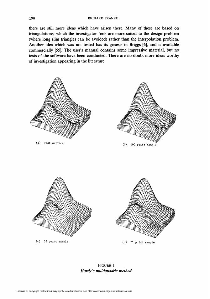
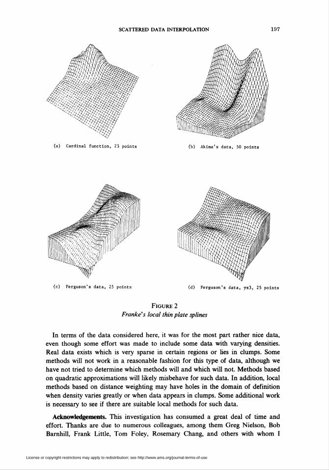
To give the flavor of the type of visual information included in the report, two
pages are reproduced here in Figures 1 and 2. Figure 1 gives the test surface in part
(a) and reconstructions of it by the multiquadric method for three different data
sets with 100, 33, and 25 points in parts (b), (c), and (d), respectively. Figure 2
shows surfaces generated by the rectangle based blending method due to the
author, using thin plate splines as the local approximations. Part (a) is a cardinal
function, part (b) was generated from Akima's data, and parts (c) and (d) were
generated from Ferguson's data. As a general rule, the best global methods seem to
result in surfaces which are visually more pleasant than those obtained from local
methods, as though localizing the surface loses something, which, while small, is
still significant in that respect. Poor behavior near edges of the data set is more
prevalent for local methods. For data sets of up to 100-200 points, global methods
are feasible and should be considered. Nielson's minimum norm network can
probably be used on somewhat larger sets of data since the sparse system of
equations is solved by iteration, while other global methods generally require
solution of a full system of N or more equations. Choice of a method for a large
number of points is to a certain extent a personal matter, but the previously
mentioned Modified Quadratic Shepard's Method performs well, requires mod-
erate storage and computation time, and is relatively easy to implement. It is also
easily extended to more independent variables. The triangle based programs, of
which Akima's is the most readily available, require considerable machinery and
storage for the triangulation, but in the end they are quite fast (Akima's being by
far the fastest of all tested methods). These methods are extremely difficult (if not
impossible) to extend to more than two independent variables and have other
previously mentioned potential defects.
Despite the number of ideas explored and programs written or obtained from
authors, and tested, there are still some which were not investigated. In addition to
the two methods from the CAGD group at Utah, which were recently obtained,
License or copyright restrictions may apply to redistribution; see http://www.ams.org/journal-terms-of-use
196 RICHARD FRANKE
there are still more ideas which have arisen there. Many of these are based on
triangulations, which the investigator feels are more suited to the design problem
(where long slim triangles can be avoided) rather than the interpolation problem.
Another idea which was not tested has its genesis in Briggs [6], and is available
commercially [55]. The user's manual contains some impressive material, but no
tests of the software have been conducted. There are no doubt more ideas worthy
of investigation appearing in the literature.
(c) 33 point sample (d) 25 point sample
Figure 1
Hardy's multiquadric method
License or copyright restrictions may apply to redistribution; see http://www.ams.org/journal-terms-of-use
SCATTERED DATA INTERPOLATION 197
(a) Cardinal function, 25 points (b) Akima's data, 50 points
(c) Ferguson's data, 25 points (d) Ferguson's data, yx3, 25 points
Figure 2
Franke''s local thin plate splines
In terms of the data considered here, it was for the most part rather nice data,
even though some effort was made to include some data with varying densities.
Real data exists which is very sparse in certain regions or lies in clumps. Some
methods will not work in a reasonable fashion for this type of data, although we
have not tried to determine which methods will and which will not. Methods based
on quadratic approximations will likely misbehave for such data. In addition, local
methods based on distance weighting may have holes in the domain of definition
when density varies greatly or when data appears in clumps. Some additional work
is necessary to see if there are suitable local methods for such data.
Acknowledgements. This investigation has consumed a great deal of time and
effort. Thanks are due to numerous colleagues, among them Greg Nielson, Bob
Barnhill, Frank Little, Tom Foley, Rosemary Chang, and others with whom I
License or copyright restrictions may apply to redistribution; see http://www.ams.org/journal-terms-of-use

198 RICHARD FRANKE
discussed many ideas and who made valuable suggestions (which were sometimes
followed!). Thanks are also due to those who supplied working programs, among
them Greg Nielson, Hiroshi Akima, Charles Lawson, Tom Foley, and Frank Little.
Very extensive use was made of the computer facility at the Naval Postgraduate
School. More recent computations have been done at the Center for Scientific
Computation and Interactive Graphics at Drexel University during the author's
sabbatical leave.
The author expresses thanks to the referees for suggestions which improved the
paper.
Department of Mathematics
Naval Postgraduate School
Monterey, California 93940
1. Hiroshi Akima, "Comments on 'Optimal contour mapping using universal kriging' by Ricardo A.
Olea," J. Geophysical Res., v. 80, 1975, pp. 832-836 (with reply).2. Hiroshi Akima, "A method of bivariate interpolation and smooth surface fitting for irregularly
distributed data points," ACM Trans. Math. Software, v. 4, 1978, pp. 148-159.3. Hiroshi Akima, "Algorithm 526: Bivariate interpolation and smooth fitting for irregularly
distributed data points," ACM Trans. Math. Software, v. 4, 1978, pp. 160-164.
4. R. E. Barnhill, "Representation and approximation of surfaces," in Mathematical Software III
(J. R. Rice, Ed.), Academic Press, New York, 1977, pp. 69-120.
5. R. E. Barnhill, R. P. Dube & F. F. Little, Shepard's Surface Interpolation Formula: Properties
and Extensions, CAGD report, University of Utah, 1980.
6. Ian C. Briggs, "Machine contouring using minimum curvature," Geophysics, v. 39, 1974, pp.
39-48.7. Jim Brown, Peter Dube & Frank Little, Smooth Interpolation with Vertex Functions
(manuscript).
8.1. K. Cratn & B. K. Bhattacharyya, "Treatment of nonequispaced two dimensional data with a
digital computer," Geoexploration, v. 5, 1967, pp. 173-194.
9. Jean Duchon, Fonctions—Spline du Type Plaque Mince en Dimencion 2, Report #231, Univ. of
Grenoble, 1975.10. Jean Duchon, Fonctions—Spline à Energie Invariate par Rotation, Report #27, Univ. of
Grenoble, 1976.11. Jean Duchon, "Interpolation des fonctions de deux variables suivant le principe de la flexion des
plaques minces," R.A.l.R.O. Anal. Numér., v. 10, 1976, pp. 5-12.
12. Jean Duchon, "Splines minimizing rotation invariant semi-norms in Sobolev spaces," in Construc-
tive Theory of Functions of Several Variables (W. Schempp and K. Zeller, Eds.), Lecture Notes in Math.
Vol. 571, Springer-Verlag, Berlin and New York, 1977, pp. 85-100.13. James C. Ferguson, "Multivariable curve interpolation," /. Assoc. Comput. Mach., v. 11, 1964,
pp. 221-228.14. Thomas Alfred Foley, Jr., Smooth Multivariate Interpolation to Scattered Data, Ph. D. Disserta-
tion, Arizona State University, 1979.
15. Thomas A. Foley & Gregory M. Nielson, "Multivariate interpolation to scattered data using
delta iteration," in Approximation Theory III (E. W. Cheney, Ed.), Academic Press, New York, 1980, pp.
419-424.16. Richard Franke, "Locally determined smooth interpolation at irregularly spaced points in
several variables," J. Inst. Math. Appl., v. 19, 1977, pp. 471-482.17. Richard Franke, Smooth Surface Approximation by a Local Method of Interpolation at Scattered
Points, Naval Postgraduate School, NPS-53-78-002, 1978.18. Richard Franke, A Critical Comparison of Some Methods for Interpolation of Scattered Data,
Naval Postgraduate School, TR #NPS-53-79-003, 1979. (Available from NTIS, # AD-A081 688/4.)19. Richard Franke & Gregory Nielson, "Smooth interpolation of large sets of scattered data,"
Internat. J. Numer. Methods Engrg., v. 15, 1980, pp. 1691-1704.20. C. M. Gold, J. D. Charters & J. Ramsden, "Automated contour mapping using triangular
element data structures and an interpolant over each irregular triangular domain," Comput. Graphics,
v. 11, 1977, pp. 170-175.
License or copyright restrictions may apply to redistribution; see http://www.ams.org/journal-terms-of-use

SCATTERED DATA INTERPOLATION 199
21. William J. Gordon & James A. Wixom, "Shepard's method of "metric interpolation" to bivariate
and multivariate interpolation," Math. Comp., v. 32, 1978, pp. 253-264.
22. R. L. Harder & R. N. Desmarais, "Interpolation using surface splines," J. Aircraft, v. 9, 1972,
pp. 189-191.23. Rolland L. Hardy, "Multiquadric equations of topography and other irregular surfaces," J.
Geophys. Res., v. 76, 1971, pp. 1905-1915.24. Rolland L. Hardy, "Analytical topographic surfaces by spatial intersection," Photogrammetric
Engineering, v. 38, 1972, pp. 452-458.25. Rolland L. Hardy, "Research results in the application of multiquadric equations to surveying
and mapping problems," Surveying and Mapping, v. 35, 1975, pp. 321-332.
26. Rolland L. Hardy, Geodetic Applications of Multiquadric Equations, Iowa State Univ. TR
# 76245 (NTIS PB 255296), 1976.
27. Rolland L. Hardy, "Least squares prediction," Photogrammetric Eng. and Remote Sensing, v. 43,
1977, pp. 475-492.
28. Rolland L. Hardy, 77ie Application of Multiquadric Equations and Point Mass Anomaly Models to
Crustal Movement Studies, NOAA TR NOS 76, NGS 11, 1978.29. Rolland L. Hardy & W. M. Gopfert, "Least squares prediction of gravity anomalies, geoidal
undulations, and deflections of the vertical with multiquadric harmonic functions," Geophys. Res.
Utters, v. 10, 1975, pp. 423-426.30. J. R. Jancaitus & J. L. Junkins, "Modeling irregular surfaces," Photogrammetric Eng. and Remote
Sensing, v. 39, 1973, pp. 413-420.
31. J. R. Jancaitus & J. L. Junkins, "Modeling in n dimensions using a weighting function
approach," J. Geophys. Res., v. 79, 1974, pp. 3361-3366.32. J. L. Junkins, G. W. Miller & J. R. Jancaitus, "A weighting function approach to modeling of
irregular surfaces," J. Geophys. Res., v. 78, 1973, pp. 1794-1803.
33. P. Lancaster, "Moving weighted least-squares methods," in Polynomial and Spline Approximation
(B. N. Sahney, Ed.), Reidel, Dordrecht, 1979, pp. 103-120.34. P. Lancaster & K. Salkauskas, Surfaces Generated by Moving Least Squares Methods, Research
Paper No. 438, Dept. of Math, and Stat., The Univ. of Calgary, Calgary, Alberta, Canada, 1979..
35. C. L. Lawson, "Software for C1 surface interpolation," in Software III (J. R. Rice, Ed.),
Academic Press, New York, 1977, pp. 159-192.
36. Frank Little, CAGD report, University of Utah. (Forthcoming.)
37. A. Maréchal & J. Serra, "Random kriging," in Geostatistics (Daniel F. Merriam, Ed.), Plenum
Press, New York, 1970, pp. 91-112.
38. G. Matheron, "Random functions and their applications in geology," in Geostatistics (Daniel F.
Merriam, Ed.), Plenum Press, New York, 1970, pp. 79-87.
39. G. Matheron, "The intrinsic random functions and their applications," Adv. in Appl. Probab.,
v. 5, 1973, pp. 439-468.40. A. D. Maude, "Interpolation—Mainly for graph plotters," Comput. J., v. 16, 1973, pp. 64-65.
41. Dermot H. McLain, "Drawing contours from arbitrary data points," Comput. J., v. 17, 1974, pp.
318-324.42. Dermot H. McLain, "Two dimensional interpolation from random data," Comput. J., v. 19, 1976,
pp. 178-181; also errata, ibid., v. 19, 1976, p. 384.43. Jean Meinguet, "Multivariate interpolation at arbitrary points made simple," Z. Angew. Math.
Phys., v. 30, 1979, pp. 292-304.44. Jean Meinguet, "An intrinsic approach to multivariate spline interpolation at arbitrary points,"
in Polynomial and Spline Approximation (B. N. Sahney, Ed.), Reidel, Dordrecht, 1979, pp. 163-190.
45. G. M. Nielson, "Minimum norm interpolation in triangles," S1AM J. Numer. Anal., v. 17, 1980,
pp. 44-62.46. Gregory M. Nielson, A Method for Interpolating Scattered Data Based Upon a Minimum
Network. (Manuscript.)
47. Ricardo O. Olea, "Optimal contour mapping using universal kriging," J. Geophys. Res., v. 79,
1974, pp. 695-702.
48. Chester R. Pelto, Thomas A. Elkins & H. A. Boyd, "Automatic contouring of irregularly
spaced data," Geophysics, v. 33, 1968, pp. 424-430.
49. M. J. D. Powell & M. A. Sabin, "Piecewise quadratic approximation on triangles," ACM Trans.
Math. Software, v. 3, 1977, pp. 316-325.50. Jean-Michel Rendu, "Disjunctive kriging: Comparison of theory with actual results," Math.
Geol., v. 12, 1980, pp. 305-320.
License or copyright restrictions may apply to redistribution; see http://www.ams.org/journal-terms-of-use

200 RICHARD FRANKE
51. M. A. Sabin, "Contouring—A review of methods for scattered data," in Mathematical Methods in
Computer Graphics and Design (K. W. Brodlie, Ed.), Academic Press, New York, 1980, pp. 63-85.
52. L. L. Schumaker, "Fitting surfaces to scattered data," in Approximation Theory II (G. G. Lorentz,
C. K. Chui & L. L. Schumaker, Eds.), Academic Press, New York, 1976, pp. 203-268.53. Donald Shepard, A Two-Dimensional Interpolation Function for Irregularly Spaced Data, Proc.
23rd Nat. Conf. ACM, 1968, pp. 517-523.54. W. L. ViTTrrow, Interpolation to Arbitrarily Spaced Data, Ph. D. Dissertation, Dept. of Math.,
Univ. of Utah, 1978.55. User Manual for "Surface Gridding Ubrary", Dynamic Graphics, 2150 Shattuck Avenue, Berkeley,
Calif., 1978.
License or copyright restrictions may apply to redistribution; see http://www.ams.org/journal-terms-of-use


![Spatial interpolation of scattered geoscientific data · transferring spatial interpolation algorithms onto the GPU [4,5,9] show promising results. 2 Inverse distance interpolation](https://img.pdfslide.us/doc/110x75/5fb28058a273d35ef842289b/spatial-interpolation-of-scattered-geoscientiic-data-transferring-spatial-interpolation.jpg)