SCAT Mobility Grant Report

MQ-RBF Meshless Method for solving CFD problems using an

Object-Oriented Approach

byLuis M. de la Cruz

National Autonomous University of Mexico (UNAM)

Supervisor: Dr. David Emerson,Computational Engineering Group, STFC-CSED,

Daresbury Laboratory, UK

June 9, 2008

Abstract

Radial Basis Functions (RBF) are well-known as powerful tools for multivariate interpolation from scattereddata. Just very recently, RBFs have gained enormous popularity in mesh-free methods for Partial DifferentialEquations (PDEs). First known applications of RBFs in Computational Fluid Dynamics (CFD) are those fromEdward Kansa in 1990, and nowadays this technique has been succesfully used in several practical problems.Various authors have been proved that the Multiquadric (MQ) kernel enjoy exponential convergence. On theother hand, the primary disadvantage of the direct MQ-RBF scheme is that it is global, hence the coefficientmatrices obtained from this discretization scheme become full and progressively more ill-conditioned as therank increases. The ill-conditioning problem has been addressed in various works and there exist severalways to improve the condition number of the coefficient matrices. The techniques include the construction ofspecial preconditioners and the use of Domain Decomposition methods (DD). In this work, the unsymmetriccollocation RBF mesh-less method is used to solve typical CFD benchmarks and the principal characteristicsof MQ-RBF are studied. To this end, a framework using the Object-Oriented Paradigm (OOP) in combinationwith the C++ language was constructed. Currently this tool contains classes for generation of points in simplegeometries, Thin-Plate Splines (TPS) and MQ RBF kernels, GMRES and Gauss elimination solvers, ACBFpreconditioner, KDTree algorithm and classes for solving problems with the alternating Schwartz domaindecomposition method in multiprocessor architectures via the use of the MPI library. Solution of Poissonequation, advection-diffusion in 1D and 2D, and incompressible viscous flows problems are presented.

1

Contents

1 Introduction 3

2 Radial Basis Functions Meshless Method 5

2.1 RBF definition . . . . . . . . . . . . . . . . . . . . . . . . . . . . . . . . . . . . . . . . . . . . . 52.2 Interpolation with RBF . . . . . . . . . . . . . . . . . . . . . . . . . . . . . . . . . . . . . . . . 62.3 Solving PDEs with RBFs . . . . . . . . . . . . . . . . . . . . . . . . . . . . . . . . . . . . . . . 6

2.3.1 Polynomial precision . . . . . . . . . . . . . . . . . . . . . . . . . . . . . . . . . . . . . . 72.4 Ill-conditioned linear systems . . . . . . . . . . . . . . . . . . . . . . . . . . . . . . . . . . . . . 8

2.4.1 The GMRES iterative method . . . . . . . . . . . . . . . . . . . . . . . . . . . . . . . . 92.4.2 Approximated Cardinal Basis Functions Preconditioner . . . . . . . . . . . . . . . . . . 92.4.3 Domain Decomposition: Additive Schwarz Method . . . . . . . . . . . . . . . . . . . . . 11

3 OOPS: Object-Oriented Programming for Scientific Computing 14

3.1 Software developing process . . . . . . . . . . . . . . . . . . . . . . . . . . . . . . . . . . . . . . 153.2 Template Units for Numerical Applications : RBF method . . . . . . . . . . . . . . . . . . . . . 15

4 CFD examples 17

4.1 Poisson equation in 2D . . . . . . . . . . . . . . . . . . . . . . . . . . . . . . . . . . . . . . . . . 174.1.1 MQ-RBF: Uniform distribution . . . . . . . . . . . . . . . . . . . . . . . . . . . . . . . . 194.1.2 MQ-RBF: Random distribution . . . . . . . . . . . . . . . . . . . . . . . . . . . . . . . . 204.1.3 MQ-RBF: Points near the boundary . . . . . . . . . . . . . . . . . . . . . . . . . . . . . 214.1.4 Shape parameter . . . . . . . . . . . . . . . . . . . . . . . . . . . . . . . . . . . . . . . . 22

4.2 Laplace equation in a Semi-circle . . . . . . . . . . . . . . . . . . . . . . . . . . . . . . . . . . . 234.3 Linear time-dependent advection-diffusion in 1D . . . . . . . . . . . . . . . . . . . . . . . . . . 254.4 Forced Convection in 2D . . . . . . . . . . . . . . . . . . . . . . . . . . . . . . . . . . . . . . . . 274.5 Lid-driven cavity . . . . . . . . . . . . . . . . . . . . . . . . . . . . . . . . . . . . . . . . . . . . 304.6 Backward-facing step . . . . . . . . . . . . . . . . . . . . . . . . . . . . . . . . . . . . . . . . . . 354.7 Domain Decomposition . . . . . . . . . . . . . . . . . . . . . . . . . . . . . . . . . . . . . . . . 37

5 Concluding remarks 38

2

1 Introduction

CFD is the analysis of systems involving fluid flow, heat transfer and asssociated phenomena such as chemicalreactions by means of computer-based simulation. CFD codes are structured around the numerical algorithmsthat can tackle fluid flow problems. A typical CFD modelling involves three principal steps: (1) TheoreticalModel, where physical laws are applied to describe the studied phenomenon in terms of a set of mathematicalequations, (2) Discrete Model, where the equations are written in terms of simple algebraic operations and (3)Solution of the resultant linear systems.

In the second step of this process it is required to decide the manner in which the governing equationswill be discretized in order to obtain approximated solutions. In the past four decades numerical simulationin CFD has been dominated by either finite difference methods (FDM), finite element methods (FEM), andfinite volume methods (FVM), which require a mesh to support the localized approximations. Typically, thesimulations are done in complicated two and three-dimensional geometries, in such a way that the constructionof a mesh in these domains is a non-trivial problem, and more than the 70% of overall computation is spentby mesh generators.

In the last decade, the so-called meshless methods for PDEs has been intensely studied because its ability ofdealing with PDEs in complex domains without a mesh at all. The popular meshless methods include movingleast square method [1, 2], generalized finite element method [3] and radial basis function (RBF) [4, 5, 6].

In 1982 Franke [7] compared 29 interpolation methods with analytic two-dimensional test functions. Accord-ingly, one of the most powerful methods is the continuously differentiable multiquadric MQ-RBF, discovered byHardy [8, 9]. The MQ-RBF for the interpolation problem has been shown by various authors to possess somevery powerful properties. Madych and Nelson [10] proved that interpolation with the MQ-RBF is exponentiallyconvergent.

In 1990, Kansa [4, 5] modified Hardys MQ method [9] to solve partial differential equations. Since then,solving PDEs using RBFs has been used for different sort of applications. Fedoseyev et al. [11] demonstratedthat the solutions of elliptic PDEs converge exponentially requiring orders of magnitude less points and opera-tions than FDM, FEM and FVM. The main advantages of the MQ-RBF scheme over the traditional methodsare that enjoys superior convergence rates, requires less points and is easy to implement in more than onedimensions. On the other side, the principal disadvantage of applying MQ-RBFs to PDE systems is that theresulting coefficient matrix can become quite ill-conditioned as N , the rank of the matrix, increases.

The cost of increasing the accuracy via RBF is usually the ill-conditioning of the associated linear systemsthat need to be solved: better conditioning is associated with poorer accuracy and worse condition-

ing is associated with improved accuracy. Different approaches have already been proposed to overcomethe difficulties, see for example [12, 13, 14, 15, 16, 17, 18, 19]. In these works several ideas are proposed:

• Domain Decomposition Methods (DDMs).

• Use of Krylov solvers (CG, GMRES, etc.) in conjunction with simple and specialized preconditioners.

• Use of a variable shape parameter as a function of the local radius of curvature.

• Use of truncated MQ basis function.

• Optimization of knots distribution.

• Multilevel approximation schemes developed by Fasshauer and Jerome [20], to keep the band-widthconstant, but refine spatial regions to the desired degree of accuracy.

Particularly, in [14] and [19] two specialized preconditioners for improving the condition number of thematrices are studied. In these two works a preconditioner is constructed using Approximated Cardinal BasisFunctions (ACBF). Brown et al. [21] compares both preconditioners and found that the LS-ACBF from [19]

3

is relatively easy to setup and performs better for very bad conditioned matrices. Also it works better fortime-dependent problems. The comparison were made in terms of GMRES iterations.

Tipically, when MQ-RBF is applied to solve PDEs using the method from [5], we found that the error islargest near the boundary, by one or two orders of magnitude than those in the domain far from the boundary.A method that improves the error near the boundary is proposed in [11], resulting in a better global accuracy.The main idea is to add an aditional set of points adjacent to the boundary (inside or outside) and, an additionalset of collocations equations obtained via collocation of the PDE on the boundary. Adding nodes near theboundary may give rise to troublesome issues and the solution depends on the distribution of this additional setof points. Similarly, when Neumann boundary conditions are imposed the accuracy is poorer compared withpure Dirichlet boundary conditions. In [22] is observed that one solution to this problem is either by refiningthe mesh size (h-scheme), or by increasing the shape parameter (c-scheme). Both schemes significantly increasethe ill-conditioning of the matrices that causes instabilities in the solution. To mitigate the ill-conditioning, animproved truncated singular value decomposition method can be used to solve the systems.

RBF mesh-less methods are recent techniques to deal with PDEs, and the typical tools for testing thesenew methods is by implementing the algorithms inside high-level frameworks like Mathlab. However, this kindof frameworks are not intended for High-Performance Computing (HPC). The main objetive in this work isto construct a framework using the C++ language in order to provide the tools for an easy developing andtesting of the RBF techniques, allowing to run the codes on HPC plataforms. The C++ language was selectedbecause it is possible to construct good and efficient object-oriented code. In general OO designs allows betterencapsulation and separation of concerns, thus providing a high degree of modularity and flexibility and greatlyincrease the potential for reuse of single systems components [23]. The fact that OOP provides these tools isnot enough to obtain good quality software, it is also necessary to use a software development process thatguides the analysis, design and implemention of the different parts of the code. A simplified software processspecially adapted for scientific computing simulations, and based on the Unified Process of Development [24]is used here. To test and calibrate the tools, a set of unit tests were defined, and these are PDEs equationscoming from CFD benchmarks. Fortran and C libraries exist that provide good performance, so the idea hereis not to redo those libraries. Instead, C++ wrappers are used to link with existent high-performance libraries.

4

2 Radial Basis Functions Meshless Method

The motivation for RBF was originated from applications in geodesy, geophysics, mapping, or meteorology.Later, applications were found in many areas such as in the numerical solution of PDEs, artificial intelligence,learning theory, neural networks, signal processing, sampling theory, statistics, finance, and optimization. Itshould be pointed out that meshfree local regression methods have been used independently in statistics formore than 100 years, see for example [25] and references therein. Recently, RBFs have been applied in solvingPDEs. The theory includes Galerkin methods [26], collocation methods [27, 28], and multilevel schemes [29].

In this section the RBFs methodology for interpolation of scattered data and for solving PDEs is introducedbriefly.

2.1 RBF definition

A radial function is defined as:

Φ : Rd → R : (~x)→ φ(||~x||) (1)

for some univariate function φ : [0,∞) → R, where ~x ∈ Rd, and || · || is the usual Euclidean norm of ~x =

(x1, . . . , xd) and is defined as:

||~x|| =

√

√

√

√

d∑

i=1

x2i (2)

The equation (1) says that the function value of Φ(x), only depends on the norm of ~x, therefore we havea radial function. If || ~x1|| = || ~x2|| then Φ( ~x1) = Φ( ~x2), for ~x1, ~x2 ∈ R

d. A useful feature of radial functions isthe fact that the interpolation problem becomes insensitive to the dimension d of the space. Instead of havingto deal with a multivariate function Φ (whose complexity will increase with the space dimension) it is possibleto work with the same univariate function φ for all choices of d.

Suppose now, we have a set of points fixed (sometimes called centers) ~xjNj=1 = ~x1, . . . , ~xN ⊂ Rd and

consider the following linear combination of the function Φ centered at the points ~xj :

u(~x) =N∑

j=1

λjΦ(~x− ~xj) =N∑

j=1

λjφ(||~x − ~xj ||) =N∑

j=1

λjφ(r) (3)

where r = ||~x − ~xj || is the Euclidean distance between the points ~x and ~xj and λjNj=1 represent a set ofunknown coefficients. The function φ is the so-called Radial Basis Function, and u is the interpolant thatapproximates the function u in a given domain.

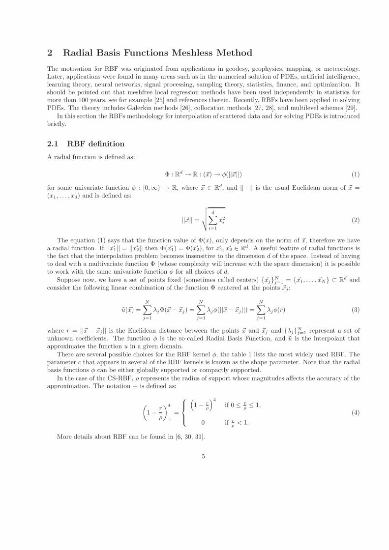
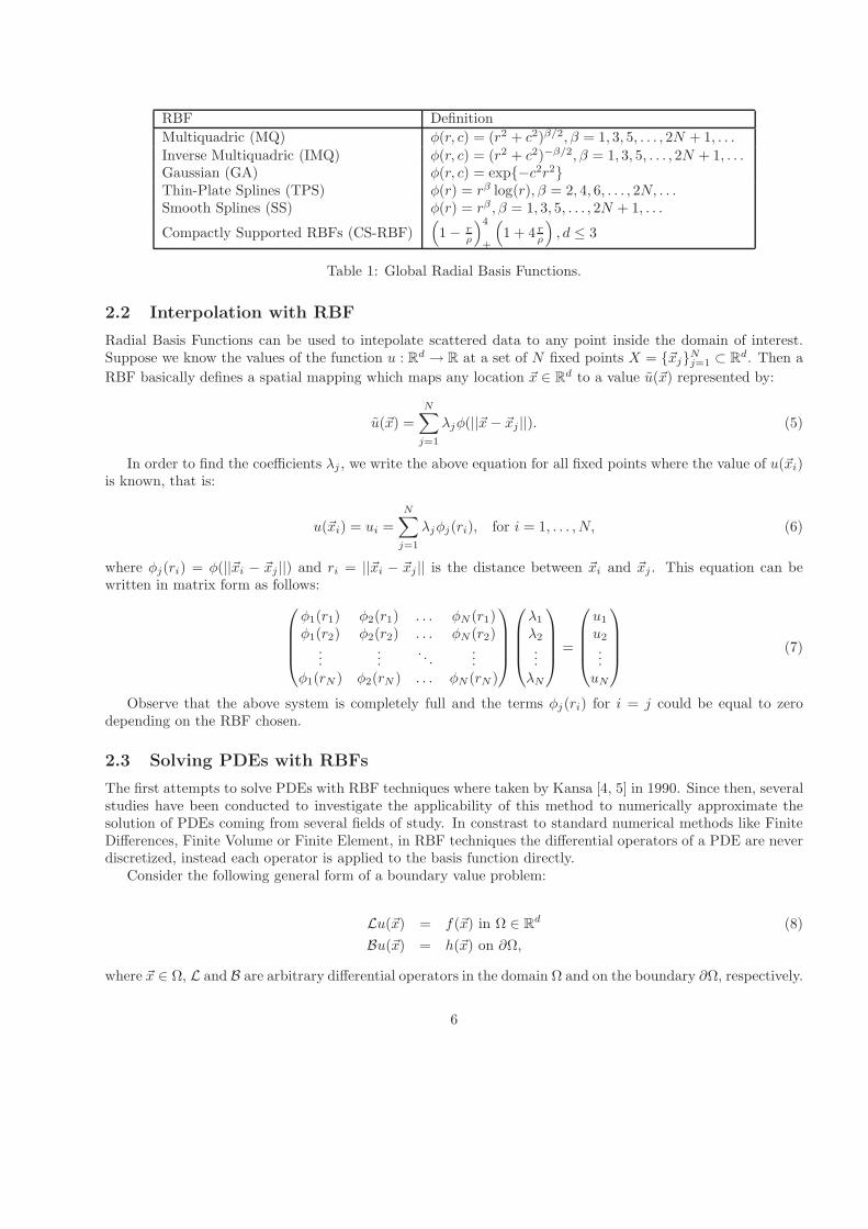
There are several possible choices for the RBF kernel φ, the table 1 lists the most widely used RBF. Theparameter c that appears in several of the RBF kernels is known as the shape parameter. Note that the radialbasis functions φ can be either globally supported or compactly supported.

In the case of the CS-RBF, ρ represents the radius of support whose magnitudes affects the accuracy of theapproximation. The notation + is defined as:

(

1− r

ρ

)4

+

=

(

1− rρ

)4

if 0 ≤ rρ ≤ 1,

0 if rρ < 1.

(4)

More details about RBF can be found in [6, 30, 31].

5

RBF Definition

Multiquadric (MQ) φ(r, c) = (r2 + c2)β/2, β = 1, 3, 5, . . . , 2N + 1, . . .

Inverse Multiquadric (IMQ) φ(r, c) = (r2 + c2)−β/2, β = 1, 3, 5, . . . , 2N + 1, . . .Gaussian (GA) φ(r, c) = exp−c2r2Thin-Plate Splines (TPS) φ(r) = rβ log(r), β = 2, 4, 6, . . . , 2N, . . .Smooth Splines (SS) φ(r) = rβ , β = 1, 3, 5, . . . , 2N + 1, . . .

Compactly Supported RBFs (CS-RBF)(

1− rρ

)4

+

(

1 + 4 rρ

)

, d ≤ 3

Table 1: Global Radial Basis Functions.

2.2 Interpolation with RBF

Radial Basis Functions can be used to intepolate scattered data to any point inside the domain of interest.Suppose we know the values of the function u : R

d → R at a set of N fixed points X = ~xjNj=1 ⊂ Rd. Then a

RBF basically defines a spatial mapping which maps any location ~x ∈ Rd to a value u(~x) represented by:

u(~x) =

N∑

j=1

λjφ(||~x − ~xj ||). (5)

In order to find the coefficients λj , we write the above equation for all fixed points where the value of u(~xi)is known, that is:

u(~xi) = ui =

N∑

j=1

λjφj(ri), for i = 1, . . . , N, (6)

where φj(ri) = φ(||~xi − ~xj ||) and ri = ||~xi − ~xj || is the distance between ~xi and ~xj . This equation can bewritten in matrix form as follows:

φ1(r1) φ2(r1) . . . φN (r1)φ1(r2) φ2(r2) . . . φN (r2)

......

. . ....

φ1(rN ) φ2(rN ) . . . φN (rN )

λ1

λ2

...λN

=

u1

u2

...uN

(7)

Observe that the above system is completely full and the terms φj(ri) for i = j could be equal to zerodepending on the RBF chosen.

2.3 Solving PDEs with RBFs

The first attempts to solve PDEs with RBF techniques where taken by Kansa [4, 5] in 1990. Since then, severalstudies have been conducted to investigate the applicability of this method to numerically approximate thesolution of PDEs coming from several fields of study. In constrast to standard numerical methods like FiniteDifferences, Finite Volume or Finite Element, in RBF techniques the differential operators of a PDE are neverdiscretized, instead each operator is applied to the basis function directly.

Consider the following general form of a boundary value problem:

Lu(~x) = f(~x) in Ω ∈ Rd (8)

Bu(~x) = h(~x) on ∂Ω,

where ~x ∈ Ω, L and B are arbitrary differential operators in the domain Ω and on the boundary ∂Ω, respectively.

6

Assume there exist N total collocation points X = ~xjNj=1 ∈ Ω, where Ω = Ω ∪ ∂Ω is known as theclosure of the domain. Define NI as the number of interior points in Ω and NB as the number of points onthe boundary ∂Ω, in such a way that N = NI +NB. By substituting equation (6) into (8) the boundary valueproblem can be written as follows:

N∑

j=1

λjLφj(~xi) = f(~xi) = fi, for i = 1, . . . , NI (9)

N∑

j=1

λjBφj(~xi) = h(~xi) = hi, for i = NI + 1, . . . , N.

To find the λj coefficients it is necessary to solve the next N ×N linear algebraic system:

Lφ1(r1) . . . LφNI(r1) LφNI+1(r1) . . . LφN (r1)

.... . .

......

. . ....

Lφ1(rNI) . . . LφNI

(rNI) LφNI+1(rNI

) . . . LφN (rNI)

Bφ1(rNI+1) . . . BφNI(rNI+1) BφNI+1(rNI+1) . . . BφN (rNI+1)

.... . .

......

. . ....

Bφ1(rN ) . . . BφNI(rN ) BφNI+1(rN ) . . . BφN(rN )

λ1

...λNI

λNI+1

...λN

=

f1...fNI

hNI+1

...hN

(10)

Defining sub-matrices WL11, WL12, WB21 and WB22

WL11 with elements Lφj(ri), for i, j = 1, . . . , NI ,WL12 with elements Lφj(ri), for i = 1, . . . , NI , j = NI + 1, . . . , N ,WB21 with elements Bφj(ri), for i = NI + 1, . . . , N , j = 1, . . . , NI ,WB22 with elements Bφj(ri), for i = NI + 1, . . . , N , j = NI + 1, . . . , N ,

and the vectors Λ = [λ1, . . . , λN )]T , F = [f1, . . . , fNI]T and H = [hN+1, . . . , gN ]T , the system (10) can be

written as follows:

G =

[

WL11 WL12

WB21 WB22

]

Λ =

[

FH

]

(11)

where G is known as the Gramm’s Matrix.The solution of system (11) give us the coefficients λj that are required to approximate u by using (5). In

principle, with this technique it is possible to find the value of u in any location inside the domain Ω.As can be observed, the collocation method with RBFs is very simple and truly mesh-less method. Also

it can be applied directly to one, two, three or more dimensions. On the other side, the matrix of the systemresult fully populated (except for the CS-RBFs), unsymmetrical and in the mostly of the cases ill-conditioned.Several authors had been addressed the ill-conditioning problem, see for example [14, 15, 16, 18, 19]. To solvethis kind of linear systems it is possible to use Gauss elimination with partial pivoting or iterative methodslike GMRES. However, Gauss elimination require O(N3) and is very expensive for many collocation points.Iterative algorithms, as in the case of GMRES, require specialized preconditioners in order to reduce the numberof iterations in generating approximated solutions in short times.

2.3.1 Polynomial precision

Sometimes the approximation given in the RBF expansion presented in equation (6) is extended by adding apolynomial as follows:

7

ui =N∑

j=1

λjφj(ri) +M∑

k=1

akpk(~xi), for i = 1, . . . , N. (12)

where the terms pk(~xi) form a basis for the M =(

d+m−1m−1

)

-dimensional linear space∏dm−1 of polynomials of

total degree less than or equal to m− 1 in d variables. The addition of a polynomial leads us to a system of Nlinear equations in N +M unknowns, therefore M additional (orthogonality) conditions are required to ensurea unique solution. These conditions are known as the moment constrains and are written as follows:

N∑

j=1

λjpk = 0, for k = 1, . . . ,M, (13)

While the use of polynomials is somewhat arbitrary, it is expected that the addition of polynomials of totaldegree at most m− 1 guarantees polynomial precision, see [6].

Substituting equation (12) in the equation (8), results in

N∑

j=1

λjLφj(~xi) +

M∑

k=1

akLpk(~xi) = f(~xi) = fi, for i = 1, . . . , NI (14)

N∑

j=1

λjBφj(~xi) +

M∑

k=1

akBpk(~xi) = h(~xi) = hi, for i = NI + 1, . . . , N.

The system (14) along with the moment constrains (13) can be written in matrix form as follows

WL PLWB PBPT 0

[

ΛA

]

=

FH~0

(15)

where A = [a1, . . . , aM ]T is the vector of coefficients for the polynomial, 0 is an M ×M matrix consisting ofzero elements, ~0 is a vector of M zero elements and:

WL is an NI ×N matrix with elements Lφj(ri), for i = 1, . . . , NI , j = 1, . . . , N ,WB is an NB ×N matrix with elements Bφj(ri), for i = NI + 1, . . . , N, j = 1, . . . , N ,PL is an NI ×M matrix with elements Lpk(~xi), for i = 1, . . . , NI , k = 1, . . . ,M ,PB is an NB ×M matrix with elements Bpk(~xi), for i = NI + 1, . . . , N, k = 1, . . . ,M .PT is an M ×N matrix with elements pk(~xi), for i = 1, . . . , N, k = 1, . . . ,M .

2.4 Ill-conditioned linear systems

The matrix systems given in (11) and (15) are generally non-symmetric and full. These systems of equationsare known to be ill-conditioned, even for moderate N . This ill-conditioning worsens with N or with a flatRBF, for example with the MQ-RBF with large shape parameter c. Although some very rare combinations ofdata center arrangements and c can produce a singular matrix, the singularity can be removed by perturbingeither the value of c or the data centers.

There is ample evidence that RBFs, especially MQ-RBFs, offers some computational advantages over tra-ditional methods, particularly is a truly mesh-free scheme that possesses very high orders rates of convergence.For small to moderate sized problems, RBFs do outperform traditional methods. The main concern is whetherRBFs can be computationally efficient with large scale, complex problems. To circumvent the ill-conditioningproblem, for large N it is possible to adapt the procedures used in large scale mesh-based PDE methods bycombining preconditioning, domain decomposition, and using parallel computers.

8

2.4.1 The GMRES iterative method

Solving large systems coming from RBF technique with non-customised methods is computationally expensive.For example, using the usual direct methods to fit an RBF with N centres requires O(N2) storage and O(N3)flops. Thus such an approach is not viable for large problems with N ≫ 10, 000. To overcome this situation,the combination of an efficient iterative algorithm and a preconditionator is required.

The GMRES iterative method for non-symmetric systems is a Krylov subspace method and its convergenceproperties parallel those of the conjugate gradient (CG) method for symmetric positive definite systems. UnlikeCG iteration, GMRES iteration requires storage of all the previous search directions, or equivalently storageof an orthonormal basis for kk, where

kk = spanr0, Ar0, . . . , Ak1r0,

and rk = b−Axk is the residual at the kth step of GMRES. In the kth iteration of GMRES xk is taken as theunique solution of the least squares problem

minx∈x0+kk

||b−Ax||2

The kth iteration of the GMRES algorithm on an N × N system requires one matrix-vector product andO(kN) additional floating point operations. The method also requires the storage of an orthonormal basis forthe Krylov subspace so that conjugate vectors can be formed at each iteration. Hence, if the total numberof iterations is K, total storage requirements, excluding any storage needed for the matrix A or computingits action, is O(KN). The corresponding flop count is K matrix-vector products and O(K2N) other floatingpoint operations. More details of the algortihm can be found in [32].

Due to its features, GMRES is one of the algorithms commonly used to solve the full systems that appearsin RBF techniques, and will be used in this work in combination with the preconditioner described in the nextsection.

2.4.2 Approximated Cardinal Basis Functions Preconditioner

Given a matrix system Gα = b as in (11), it is possible to construct a left-hand preconditioner W , and tosolve the equivalent system WGα = Wb, for the undetermined coefficients α. The application of such apreconditioner to a bad-conditioned matrix, results in clustering the eigenvalues of the matrix and thereforereducing the total number of iterations required for GMRES (or other algorithm) to converge. Using a basisof cardinal functions, see [14], which would be equivalent to a delta-function, δ(~xi) that is one at its center ~xiand zero everywhere else, would result in WG = I, where I represents the identity matrix. For this matrixGMRES would converge in one iteration. However, this is totally impractical because the preconditioner wouldneed to be exactly the matrix inverse. The strategy that is used instead, is to construct the preconditionerusing approximate cardinal basis functions (ACBF).

In this work the LS-ACBF preconditioner, proposed by Ling et al. [19] is used to improve the conditionnumbers of the linear systems. The idea in the construction of LS-ACBF preconditioner is to satisfy the abovecardinal condition in the least-squares sense. A brief description of this preconditioner is given below.

Let φI and φB denote the NI and NB RBFs whose center is in Ω and in ∂Ω respectively. The rows of thematrix G, from equation (11), are discrete function values given by:

Ψ(~x)Ni=1 = LφI(~xi − ~x)NI

i=1 ∪ BφB(~xi − ~x)NB

i=1 (16)

Each column of G has contributions from NI entries of LφI and NB entries of BφB. For each center ~xi ,select a small subset of centers or support of size m≪ N indicated by the index set

Si = [s(1)i , s

(2)i , . . . , s

(m)i ], i ∈ Si, (17)

9

such that we try to enforce the condition

∑

j∈Si

wjΨj(~x) = δ(~x), for all ~x ∈ X, (18)

where δi(~x) is one at ~xi and zero elsewhere.

The index set Si is a combination of local nearest centers to ~xi and special points distributed on the domain.Si will be the ml local nearest centers to ~xi that can be found efficiently in O(NlogN) flops, and ms specialpoints where ml +ms = m.

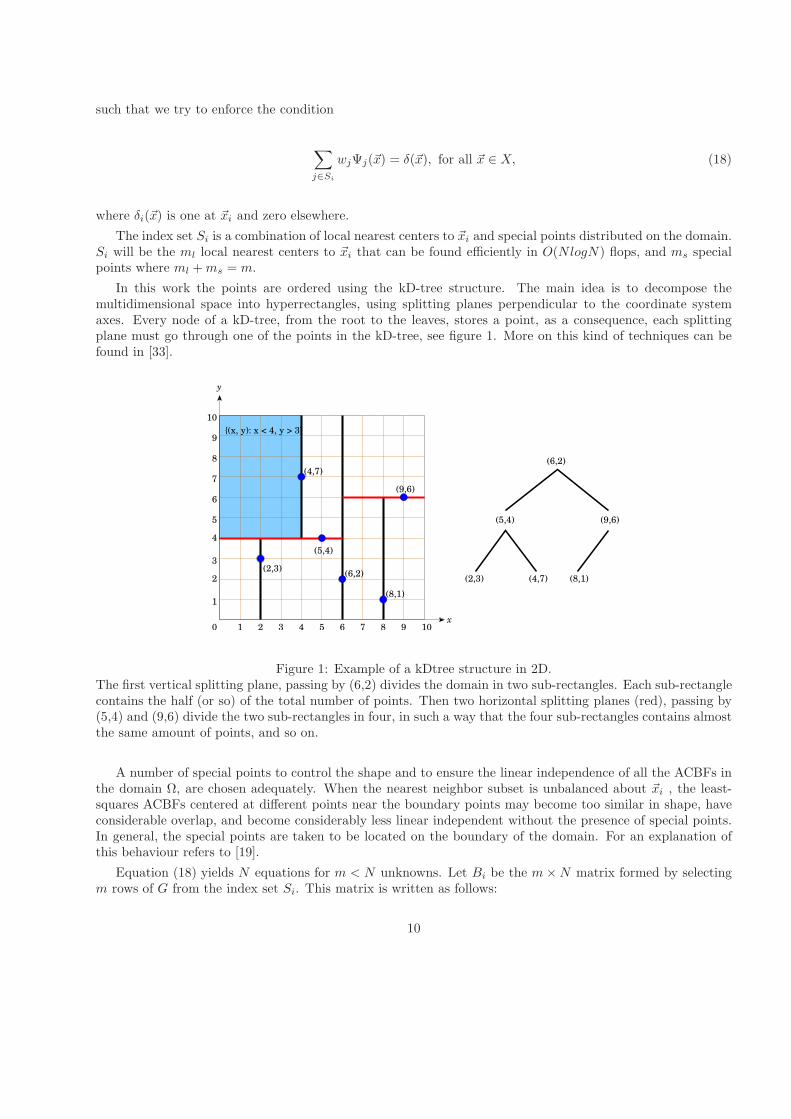
In this work the points are ordered using the kD-tree structure. The main idea is to decompose themultidimensional space into hyperrectangles, using splitting planes perpendicular to the coordinate systemaxes. Every node of a kD-tree, from the root to the leaves, stores a point, as a consequence, each splittingplane must go through one of the points in the kD-tree, see figure 1. More on this kind of techniques can befound in [33].

1

2

3

4

5

6

7

8

9

10

(2,3)

(8,1)

(5,4)

(4,7)

(6,2)

(9,6)

(8,1)

y

x1 2 3 4 5 6 7 8 9 100

(5,4) (9,6)

(6,2)

(2,3) (4,7)

(x, y): x < 4, y > 3

Figure 1: Example of a kDtree structure in 2D.The first vertical splitting plane, passing by (6,2) divides the domain in two sub-rectangles. Each sub-rectanglecontains the half (or so) of the total number of points. Then two horizontal splitting planes (red), passing by(5,4) and (9,6) divide the two sub-rectangles in four, in such a way that the four sub-rectangles contains almostthe same amount of points, and so on.

A number of special points to control the shape and to ensure the linear independence of all the ACBFs inthe domain Ω, are chosen adequately. When the nearest neighbor subset is unbalanced about ~xi , the least-squares ACBFs centered at different points near the boundary points may become too similar in shape, haveconsiderable overlap, and become considerably less linear independent without the presence of special points.In general, the special points are taken to be located on the boundary of the domain. For an explanation ofthis behaviour refers to [19].

Equation (18) yields N equations for m < N unknowns. Let Bi be the m×N matrix formed by selectingm rows of G from the index set Si. This matrix is written as follows:

10

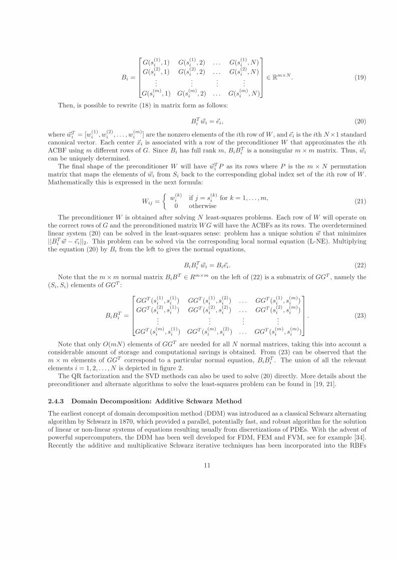
Bi =

G(s(1)i , 1) G(s

(1)i , 2) . . . G(s

(1)i , N)

G(s(2)i , 1) G(s

(2)i , 2) . . . G(s

(2)i , N)

......

......

G(s(m)i , 1) G(s

(m)i , 2) . . . G(s

(m)i , N)

∈ Rm×N . (19)

Then, is possible to rewrite (18) in matrix form as follows:

BTi ~wi = ~ei, (20)

where ~wTi = [w(1)i , w

(2)i , . . . , w

(m)i ] are the nonzero elements of the ith row of W , and ~ei is the ith N×1 standard

canonical vector. Each center ~xi is associated with a row of the preconditioner W that approximates the ithACBF using m different rows of G. Since Bi has full rank m, BiB

Ti is a nonsingular m×m matrix. Thus, ~wi

can be uniquely determined.The final shape of the preconditioner W will have ~wTi P as its rows where P is the m × N permutation

matrix that maps the elements of ~wi from Si back to the corresponding global index set of the ith row of W .Mathematically this is expressed in the next formula:

Wij =

w(k)i if j = s

(k)i for k = 1, . . . ,m,

0 otherwise(21)

The preconditioner W is obtained after solving N least-squares problems. Each row of W will operate onthe correct rows of G and the preconditioned matrix WG will have the ACBFs as its rows. The overdeterminedlinear system (20) can be solved in the least-squares sense: problem has a unique solution ~w that minimizes||BTi ~w − ~ei||2. This problem can be solved via the corresponding local normal equation (L-NE). Multiplyingthe equation (20) by Bi from the left to gives the normal equations,

BiBTi ~wi = Bi~ei. (22)

Note that the m×m normal matrix BiBT ∈ Rm×m on the left of (22) is a submatrix of GGT , namely the

(Si, Si) elements of GGT :

BiBTi =

GGT (s(1)i , s

(1)i ) GGT (s

(1)i , s

(2)i ) . . . GGT (s

(1)i , s

(m)i )

GGT (s(2)i , s

(1)i ) GGT (s

(2)i , s

(2)i ) . . . GGT (s

(2)i , s

(m)i )

......

......

GGT (s(m)i , s

(1)i ) GGT (s

(m)i , s

(2)i ) . . . GGT (s

(m)i , s

(m)i )

. (23)

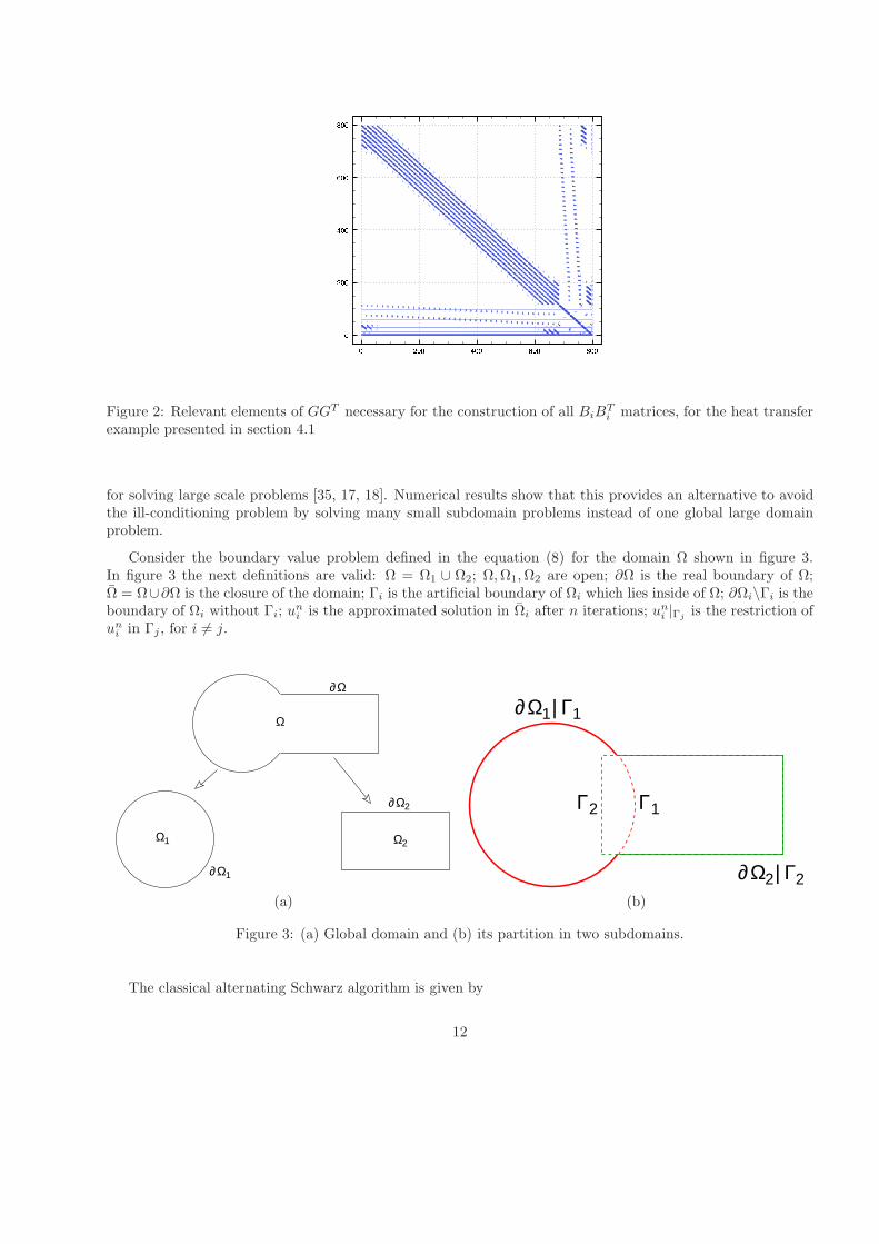
Note that only O(mN) elements of GGT are needed for all N normal matrices, taking this into account aconsiderable amount of storage and computational savings is obtained. From (23) can be observed that them × m elements of GGT correspond to a particular normal equation, BiB

Ti . The union of all the relevant

elements i = 1, 2, . . . , N is depicted in figure 2.The QR factorization and the SVD methods can also be used to solve (20) directly. More details about the

preconditioner and alternate algorithms to solve the least-squares problem can be found in [19, 21].

2.4.3 Domain Decomposition: Additive Schwarz Method

The earliest concept of domain decomposition method (DDM) was introduced as a classical Schwarz alternatingalgorithm by Schwarz in 1870, which provided a parallel, potentially fast, and robust algorithm for the solutionof linear or non-linear systems of equations resulting usually from discretizations of PDEs. With the advent ofpowerful supercomputers, the DDM has been well developed for FDM, FEM and FVM, see for example [34].Recently the additive and multiplicative Schwarz iterative techniques has been incorporated into the RBFs

11

0 2 0 0 4 0 0 6 0 0 8 0 002 0 04 0 06 0 08 0 0

Figure 2: Relevant elements of GGT necessary for the construction of all BiBTi matrices, for the heat transfer

example presented in section 4.1

for solving large scale problems [35, 17, 18]. Numerical results show that this provides an alternative to avoidthe ill-conditioning problem by solving many small subdomain problems instead of one global large domainproblem.

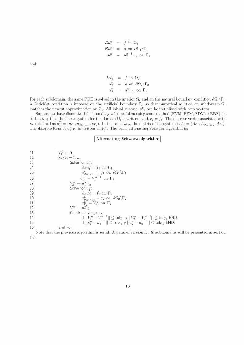
Consider the boundary value problem defined in the equation (8) for the domain Ω shown in figure 3.In figure 3 the next definitions are valid: Ω = Ω1 ∪ Ω2; Ω,Ω1,Ω2 are open; ∂Ω is the real boundary of Ω;Ω = Ω∪∂Ω is the closure of the domain; Γi is the artificial boundary of Ωi which lies inside of Ω; ∂Ωi\Γi is theboundary of Ωi without Γi; u

ni is the approximated solution in Ωi after n iterations; uni |Γj

is the restriction ofuni in Γj , for i 6= j.

Ω1

Ω1∂

Ω∂

Ω

Ω2

Ω2∂

∂ | Γ1Ω1

∂ | Γ2Ω2

Γ1Γ2

(a) (b)

Figure 3: (a) Global domain and (b) its partition in two subdomains.

The classical alternating Schwarz algorithm is given by

12

Lun1 = f in Ω1

Bun1 = g on ∂Ω1\Γ1

un1 = un−12 |Γ1

on Γ1

and

Lun2 = f in Ω2

un2 = g on ∂Ω2\Γ2

un2 = un1 |Γ2on Γ2

For each subdomain, the same PDE is solved in the interior Ωi and on the natural boundary condition ∂Ωi\Γi.A Dirichlet condition is imposed on the artificial boundary Γi, so that numerical solution on subdomain Ωimatches the newest approximation on Ωi. All initial guesses, u0

i , can be initialized with zero vectors.Suppose we have discretized the boundary value problem using some method (FVM, FEM, FDM or RBF), in

such a way that the linear system for the domain Ωi is written as Aiui = fi. The discrete vector asociated withui is defined as uTi = (uΩi

, u∂Ωi\Γi, uΓi

). In the same way, the matrix of the system is Ai = (AΩi, A∂Ωi\Γi

, AΓi).

The discrete form of uni |Γjis written as V nj . The basic alternating Schwarz algorithm is:

Alternating Schwarz algorithm

.01 V 0

1 ← 0.02 For n = 1, ...03 Solve for un1 :04 A1u

n1 = f1 in Ω1

05 un∂Ω1\Γ1= g1 on ∂Ω1\Γ1

06 unΓ1= V n−1

1 on Γ1

07 V n2 ← un1 |Γ2

08 Solve for un2 :09 A2u

n2 = f2 in Ω2

10 un∂Ω2\Γ2= g2 on ∂Ω2\Γ2

11 unΓ2= V n2 on Γ2

12 V n1 ← un2 |Γ1

13 Check convergency:14 If ||V n1 − V n−1

1 || ≤ tolΓ1y ||V n2 − V n−1

2 || ≤ tolΓ2END.

15 If ||un1 − un−11 || ≤ tolΩ1

y ||un2 − un−12 || ≤ tolΩ2

END.16 End For

Note that the previous algorithm is serial. A parallel version for K subdomains will be presented in section4.7.

13

3 OOPS: Object-Oriented Programming for Scientific Computing

Scientific computing has changed dramatically within the last decades reaching an unprecedented degree ofcomplexity. The vast advances made in the development of new hardware architectures and modern numericalmethods provide us with tools to tackle more and more complex problems. As a result, certain scientific prob-lems can be simulated with a very good accuracy and nowadays, scientific computing has become indispensablein many fields, such as engineering, science, and even in social sciences and medicine. The coding of complexnumerical algorithms need to be portable and efficient in order to achieve good performance on the majority ofavailable hardware resources. Consequently, the design and development of software is an essential componentwithin scientific computing, and requires an interdisciplinary cooperation of experts from several areas of study.

Sophisticated algorithms, a wide range of large-scale hardware environments, and an increasing demand forsystem integration and portability have shown that language level abstraction must be increased without lossof performance. Using numerical methods and reference implementations from popular textbooks is often notsufficient for the development of serious scientific software. In a similar way, the use of high-level programminglanguages contained in tools like Mathlab, can support the initial development of new numerical methodsand the rapid implementation of prototypes. However, these packages are not sufficient as High-PerformanceComputing (HPC) kernels and neither are they intended for this purpose.

The traditional paradigm for writing scientific software is known as structured where the code is separatedinto subroutines and/or functions that can be called from a main program. The common languages used areFortran (77 and 90) and C. While tens of thousands of lines of structured Fortran code may be understandable,as algorithms develop in complexity, and programs stretch to hundreds of thousands of lines, more attentionwill need to be paid to the software development process. In many cases there is relatively little sharing ofscientific code (i.e. software reuse), and scientific codes tend to be extremely specialized. Most codes implementa single method; if a different method is required, usually a new program is written. This can be extreme:often a different program will exist for each system studied.

Solutions to these problems are known. They were developed by computer scientists when the businessworld suffered its software crisis in the 1980s. Techniques such as object-oriented programming and genericprogramming are now well established, and have proven themselves. They are even starting to penetratescientific fields.

The Object-Oriented paradigm exhibit powerful features like abstraction, classes, inheritance and polymor-phism, that can ease the development, maintainability, extensibility and usability of complex software. In OOP,a program is broken down into largely independent pieces, interacting via well-defined interfaces. Writing alarge OO program is similar to writing lots of small programs, and the implementation of each part can bechanged without fear of breaking the whole package. Because OO software tends to be better organized, thereare more opportunities for code reuse. Instead of writing a completely new program, a new method can beimplemented into a class, then objects of these classes interact with other objects to solve a problem using thenew method. Extending an OO program often only requires a few lines of existing code to be changed.

Notwithstanding, mostly of scientific libraries are still implemented in non-object-oriented languages. Themain reason of this fact is because the abstractions generally result in a runtime overhead that is sometimeshard to avoid. In HPC, C++ used to have a bad reputation due to a bad runtime performance. However,C++ provides generic programming, via the use of templates [36], which allows high performance code to bewritten, without sacrificing expressiveness. Generic programming allows code to be written for generic types;the types used are determined at compile time, allowing the compiler to perform aggressive optimizations.Other techniques, like Metaprogramming [37] and Expression templates [38], help to get good performance aswell. There are presently several examples where C++, OOP and generic programming have been used in theconstruction of new frameworks for scientific computing applications. Some real and succesful libraries can befound in [39].

14

3.1 Software developing process

Scientific software is typically written with little attention paid to design. For small programs, this is often thefastest route to results, but as software grows over time, it is difficult for programmers to maintain such codesand to add new features.

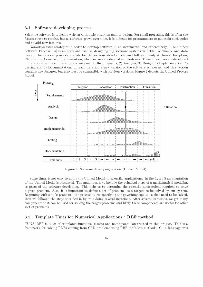
Nowadays exist strategies in order to develop software in an incremental and ordered way. The UnifiedSoftware Process [24] is an standard used in designing big software systems in fields like finance and databases. This process provides a guide for the software development and follows mainly 4 phases: Inception,Elaboration, Construction y Transition, which in turn are divided in milestones. These milestones are developedin iterations, and each iteration consists on: 1) Requirements, 2) Analysis, 3) Design, 4) Implementation, 5)Testing and 6) Documentation. In each iteration a new version of the software is released and this versioncontains new features, but also must be compatible with previous versions. Figure 4 depicts the Unified ProcessModel.

Documentation

1 2 3 4 5 ... ... ... ... ... ... ... ...... n−1 n

Inception Elaboration Construction Transition

Iterations

Phases

Ste

ps

Testing

Analysis

Requirements

Design

Implementación

Iteration

Figure 4: Software developing process (Unified Model).

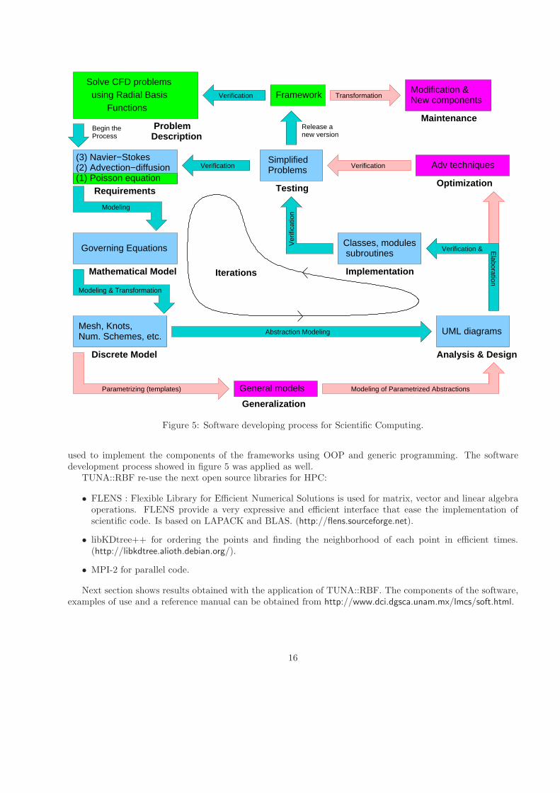
Some times is not easy to apply the Unified Model to scientific applications. In the figure 5 an adaptationof the Unified Model is presented. The main idea is to include the principal steps of a mathematical modelingas parts of the software developing. This help us to determine the essential abstractions required to solvea given problem. Also, it is important to define a set of problems as a targets to be solved by our system.Beginning with simple problems, the process starts specifying the governing equations that need to be solved,then we followed the steps specified in figure 5 doing several iterations. After several iterations, we get manycomponents that can be used for solving the target problems and likely these components are useful for othersort of problems.

3.2 Template Units for Numerical Applications : RBF method

TUNA::RBF is a set of templated functions, classes and namespaces constructed in this project. This is aframework for solving PDEs coming from CFD problems using RBF mesh-less methods. C++ language was

15

Problems

new versionRelease aBegin the

Process

Solve CFD problemsusing Radial Basis

Functions

ProblemDescription

Modeling

Mathematical Model

Governing Equations

Modeling & Transformation

Mesh, Knots,

Discrete Model

Generalization

Parametrizing (templates)

Analysis & Design

UML diagrams

Verification & Elaboration

Implementation

Classes, modulessubroutines

Ver

ifica

tion

Adv techniquesVerification Verification

Testing

Verification TransformationFramework New componentsModification &

Iterations

Num. Schemes, etc.

(1) Poisson equation(2) Advection−diffusion(3) Navier−Stokes

Requirements

Maintenance

Abstraction Modeling

Modeling of Parametrized AbstractionsGeneral models

Simplified

Optimization

Figure 5: Software developing process for Scientific Computing.

used to implement the components of the frameworks using OOP and generic programming. The softwaredevelopment process showed in figure 5 was applied as well.

TUNA::RBF re-use the next open source libraries for HPC:

• FLENS : Flexible Library for Efficient Numerical Solutions is used for matrix, vector and linear algebraoperations. FLENS provide a very expressive and efficient interface that ease the implementation ofscientific code. Is based on LAPACK and BLAS. (http://flens.sourceforge.net).

• libKDtree++ for ordering the points and finding the neighborhood of each point in efficient times.(http://libkdtree.alioth.debian.org/).

• MPI-2 for parallel code.

Next section shows results obtained with the application of TUNA::RBF. The components of the software,examples of use and a reference manual can be obtained from http://www.dci.dgsca.unam.mx/lmcs/soft.html.

16

4 CFD examples

The examples presented in this section are intended to test and calibrate the framework that has been developedduring this proyect. These examples have been instensely studied and used to test new numerical methods,and there exist a plenty number of works to compare with. The idea in this work, is to solve the PDEs of theseproblems using the asymmetric collocation RBF mesh-less method from Kansa [5] and to study the behaviorof numerical solutions under different conditions.

For all the examples that follow the Multiquadric RBF kernel for β = 1 and its derivatives are used tocalculate the numerical solution. In the mostly of the cases the shape parameter is set equal to c = 1/

√N as

is recommended in [19].

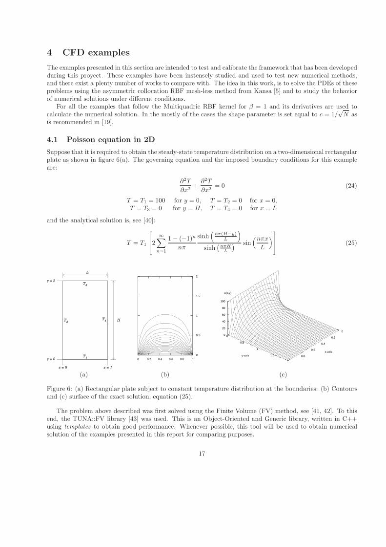
4.1 Poisson equation in 2D

Suppose that it is required to obtain the steady-state temperature distribution on a two-dimensional rectangularplate as shown in figure 6(a). The governing equation and the imposed boundary conditions for this exampleare:

∂2T

∂x2+∂2T

∂x2= 0 (24)

T = T1 = 100 for y = 0, T = T2 = 0 for x = 0,T = T3 = 0 for y = H , T = T4 = 0 for x = L

and the analytical solution is, see [40]:

T = T1

2∞∑

n=1

1− (−1)n

nπ

sinh(

nπ(H−y)L

)

sinh(

nπHL

) sin(nπx

L

)

(25)

T2

x = 0

y = 0

y = 2

x = 1

L

H

T

T

T3

4

1 0 0.2 0.4 0.6 0.8 1

0

0.5

1

1.5

2

0

0.2

0.4

0.6

0.8

x-axis

0

0.5

1

1.5y-axis

0

20

40

60

80

100

u(x,y)

(a) (b) (c)

Figure 6: (a) Rectangular plate subject to constant temperature distribution at the boundaries. (b) Contoursand (c) surface of the exact solution, equation (25).

The problem above described was first solved using the Finite Volume (FV) method, see [41, 42]. To thisend, the TUNA::FV library [43] was used. This is an Object-Oriented and Generic library, written in C++using templates to obtain good performance. Whenever possible, this tool will be used to obtain numericalsolution of the examples presented in this report for comparing purposes.

17

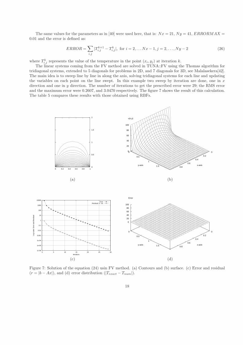
The same values for the parameters as in [40] were used here, that is: Nx = 21, Ny = 41, ERRORMAX =0.01 and the error is defined as:

ERROR =∑

i,j

|T k+1i,j − T ki,j |, for i = 2, . . .Nx− 1, j = 2, . . . , Ny − 2 (26)

where T ki,j represents the value of the temperature in the point (xi, yj) at iteration k.The linear systems coming from the FV method are solved in TUNA::FV using the Thomas algorithm for

tridiagonal systems, extended to 5 diagonals for problems in 2D, and 7 diagonals for 3D, see Malalasekera[42].The main idea is to sweep line by line in along the axis, solving tridiagonal systems for each line and updatingthe variables on each point on the line swept. In this example two sweep by iteration are done, one in xdirection and one in y direction. The number of iterations to get the prescribed error were 29; the RMS errorand the maximum error were 0.2607, and 3.0470 respectively. The figure 7 shows the result of this calculation.The table 5 compares these results with those obtained using RBFs.

0 0.2 0.4 0.6 0.8 1 0

0.5

1

1.5

2

0

0.2

0.4

0.6

0.8x-axis

0

0.5

1

1.5y-axis

0

20

40

60

80

100

u(x,y)

(a) (b)

1e-06

1e-05

1e-04

0.001

0.01

0.1

1

10

100

1000

10000

0 5 10 15 20 25 30

Log

scal

e: E

rror

and

Res

idua

l

Iterations

ErrorResidual: b - Ax

0

0.2

0.4

0.6

0.8x-axis

0

0.5

1

1.5y-axis

0

20

40

60

80

100

Error

(c) (d)

Figure 7: Solution of the equation (24) usin FV method. (a) Contours and (b) surface. (c) Error and residual(r = |b−Ax|), and (d) error distribution (|Texact − Tnum|).

18

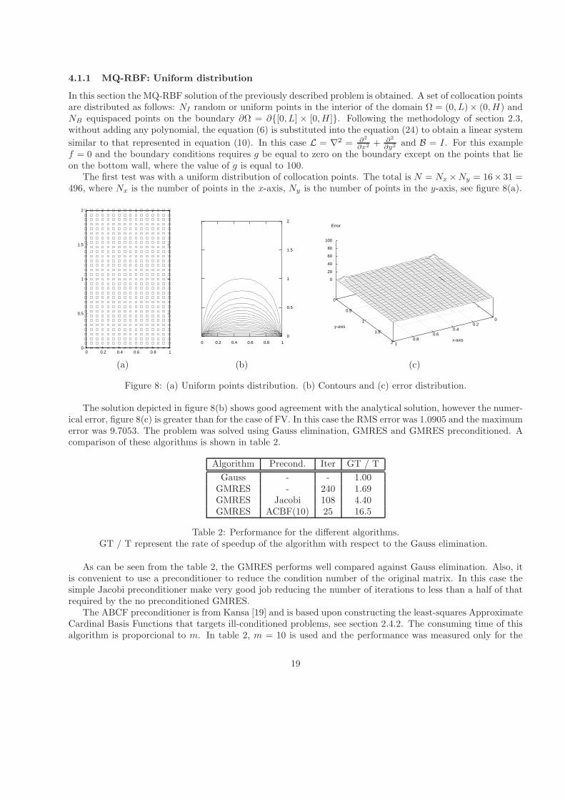
4.1.1 MQ-RBF: Uniform distribution

In this section the MQ-RBF solution of the previously described problem is obtained. A set of collocation pointsare distributed as follows: NI random or uniform points in the interior of the domain Ω = (0, L)× (0, H) andNB equispaced points on the boundary ∂Ω = ∂[0, L] × [0, H ]. Following the methodology of section 2.3,without adding any polynomial, the equation (6) is substituted into the equation (24) to obtain a linear system

similar to that represented in equation (10). In this case L = ∇2 = ∂2

∂x2 + ∂2

∂y2 and B = I. For this examplef = 0 and the boundary conditions requires g be equal to zero on the boundary except on the points that lieon the bottom wall, where the value of g is equal to 100.

The first test was with a uniform distribution of collocation points. The total is N = Nx×Ny = 16× 31 =496, where Nx is the number of points in the x-axis, Ny is the number of points in the y-axis, see figure 8(a).

0

0.5

1

1.5

2

0 0.2 0.4 0.6 0.8 1

0 0.2 0.4 0.6 0.8 1

0

0.5

1

1.5

2

0 0.2

0.4 0.6

0.8 1

x-axis

0

0.5

1

1.5

2

y-axis

0

20

40

60

80

100

Error

(a) (b) (c)

Figure 8: (a) Uniform points distribution. (b) Contours and (c) error distribution.

The solution depicted in figure 8(b) shows good agreement with the analytical solution, however the numer-ical error, figure 8(c) is greater than for the case of FV. In this case the RMS error was 1.0905 and the maximumerror was 9.7053. The problem was solved using Gauss elimination, GMRES and GMRES preconditioned. Acomparison of these algorithms is shown in table 2.

Algorithm Precond. Iter GT / T

Gauss - - 1.00GMRES - 240 1.69GMRES Jacobi 108 4.40GMRES ACBF(10) 25 16.5

Table 2: Performance for the different algorithms.GT / T represent the rate of speedup of the algorithm with respect to the Gauss elimination.

As can be seen from the table 2, the GMRES performs well compared against Gauss elimination. Also, itis convenient to use a preconditioner to reduce the condition number of the original matrix. In this case thesimple Jacobi preconditioner make very good job reducing the number of iterations to less than a half of thatrequired by the no preconditioned GMRES.

The ABCF preconditioner is from Kansa [19] and is based upon constructing the least-squares ApproximateCardinal Basis Functions that targets ill-conditioned problems, see section 2.4.2. The consuming time of thisalgorithm is proporcional to m. In table 2, m = 10 is used and the performance was measured only for the

19

GMRES iteration without taking in to account the time for constructing the preconditioner. In the table 3 thetime to calculate the preconditioner in function of m is reported.

m GMRES GMRES ACBF Precond. TotalIter. Time KDT FN LS

8 28 0.05 0.01 0.17 0.42 0.6510 25 0.04 0.01 0.21 0.39 0.6520 17 0.03 0.01 0.24 0.70 0.9830 15 0.03 0.01 0.26 1.14 1.4450 13 0.03 0.01 0.39 2.10 2.53100 10 0.03 0.01 0.46 5.77 6.27

Table 3: CPU time to construct the ACBF preconditioner. All the times are in seconds.KDT : KD-Tree construction; FN : Finding the neighbors to all the collocation points; LS : Least-square

problem solution.

From table 3 it is obvious that the consuming time for the ACBF preconditioner is not economic for largem. The total time presented in the last column would be the total time for solving the linear system includingthe construction of the preconditioner. In this case the best value of m in terms of calculation time and numberof GMRES iterations is 10.

Even though the consuming time for constructing the ACBF preconditioner is expensive for this example,in the case of time-dependent problems it could be very valuable to use this preconditioner, because for fixedcollocation points the preconditioner just needs to be calculated once at the beginning, and for every timestep the number of GMRES iterations will be reduced drastically compared with the Jacobi preconditioner.Besides, here the L-NE technique was used to solve the N- least-square problems required in the constructionof the preconditioner, but it is possible to use other optimized algorithms that can reduce the consuming times,see [19] for more details.

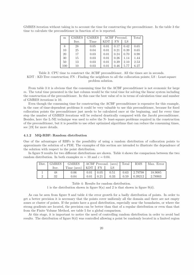
4.1.2 MQ-RBF: Random distribution

One of the advantages of RBFs is the possibility of using a random distribution of collocation points toapproximate the solution of a PDE. The examples of this section are intended to illustrate the dependence ofthe solution with respect to the point distribution.

In figure 9 results for two different distributions are shown. Table 4 shows the comparison between the tworandom distribution. In both examples m = 10 and c = 0.04.

Dist. GMRES GMRES ACBF Precond. (secs) Total RMS Max. ErrorIter. Time (secs) KDT FN LS

1 48 0.06 0.01 0.05 0.51 0.63 2.79798 18.90852 32 0.04 0.01 0.21 0.33 0.59 0.39212 2.78903

Table 4: Results for random distribution.1 is the distribution shown in figure 9(a) and 2 is that shown in figure 9(d).

As can be seen from figure 9 and table 4 the error growth for a badly distribution of points. In order toget a better precision it is necessary that the points cover uniformly all the domain and there are not emptyzones or cluster of points. If the points have a good distribution, especially near the boundaries, or where thestrong gradients are located, the precision can be better than that of a regular distribution or even than thatfrom the Finite Volume Method, see table 5 for a global comparison.

At this stage, it is important to notice the need of controlling random distribution in order to avoid badresults. The distribution of figure 9(d) was controlled allowing a point be randomly located in a limited region

20

0

0.5

1

1.5

2

0 0.2 0.4 0.6 0.8 1

0 0.2 0.4 0.6 0.8 1

0

0.5

1

1.5

2

0 0.2

0.4 0.6

0.8 1

x-axis

0

0.5

1

1.5

2

y-axis

0

20

40

60

80

100

Error

(a) (b) (c)

0

0.5

1

1.5

2

0 0.2 0.4 0.6 0.8 1

0 0.2 0.4 0.6 0.8 1

0

0.5

1

1.5

2

0 0.2

0.4 0.6

0.8 1

x-axis

0

0.5

1

1.5

2

y-axis

0

20

40

60

80

100

Error

(d) (e) (f)

Figure 9: Random distribution of collocation points for the heat transfer example.Distribution 1 : (a), (b) and (c), results for a badly distribution. Distribution 2 : (d), (e) and (f), better globalrandom distribution.

of the domain, but not on the whole domain. In this case, every point is allowed to move inside cells definedby a regular mesh.

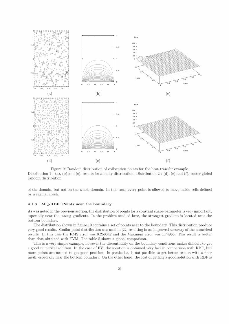
4.1.3 MQ-RBF: Points near the boundary

As was noted in the previous section, the distribution of points for a constant shape parameter is very important,especially near the strong gradients. In the problem studied here, the strongest gradient is located near thebottom boundary.

The distribution shown in figure 10 contains a set of points near to the boundary. This distribution producevery good results. Similar point distribution was used in [22] resulting in an improved accurary of the numericalresults. In this case the RMS error was 0.250542 and the Maximun error was 1.74965. This result is betterthan that obtained with FVM. The table 5 shows a global comparison.

This is a very simple example, however the discontinuity on the boundary conditions makes difficult to geta good numerical solution. In the case of FV, the solution is obtained very fast in comparison with RBF, butmore points are needed to get good pecision. In particular, is not possible to get better results with a finermesh, especially near the bottom boundary. On the other hand, the cost of getting a good solution with RBF is

21

0

0.5

1

1.5

2

0 0.2 0.4 0.6 0.8 1

0 0.2 0.4 0.6 0.8 1

0

0.5

1

1.5

2

0 0.2

0.4 0.6

0.8 1

x-axis

0

0.5

1

1.5

2

y-axis

0

20

40

60

80

100

Error

(a) (b) (c)

Figure 10: Best distribution collocation points for c = 0.04.

Case Points Iter RMS Max T / FVT

FV 861 29 0.2607 3.0470 1.0RBF 1 496 25 1.0950 9.7053 4.0RBF 2 496 48 2.7979 18.9085 6.0RBF 3 540 32 0.3921 2.7890 4.0RBF 4 540 25 0.2505 1.74965 3.0

Table 5: Global comparison for the heat transfer problem.

FVT / T is the ratio between the Finite Volume consuming time and the consuming time of the RBF method fordifferent distributions. FV: Finite Volume solution; RBF1: uniform distribution, figure 8(a); RBF2: badly ran-dom distribution, figure 9(a); RBF3: good random distribution, figure 9(d); RBF4: Best regular distribution,figure 10(a).

expensive compared with FV. However the best solution is only 3 times slower than FV. Besides the precisionis better and the implementation of RBF methods is simple: the same functions can be used for 2D and 3Dproblems. The powerful of RBF methodology should be clear when dealing with time-dependent problems andin complicated geometries.

4.1.4 Shape parameter

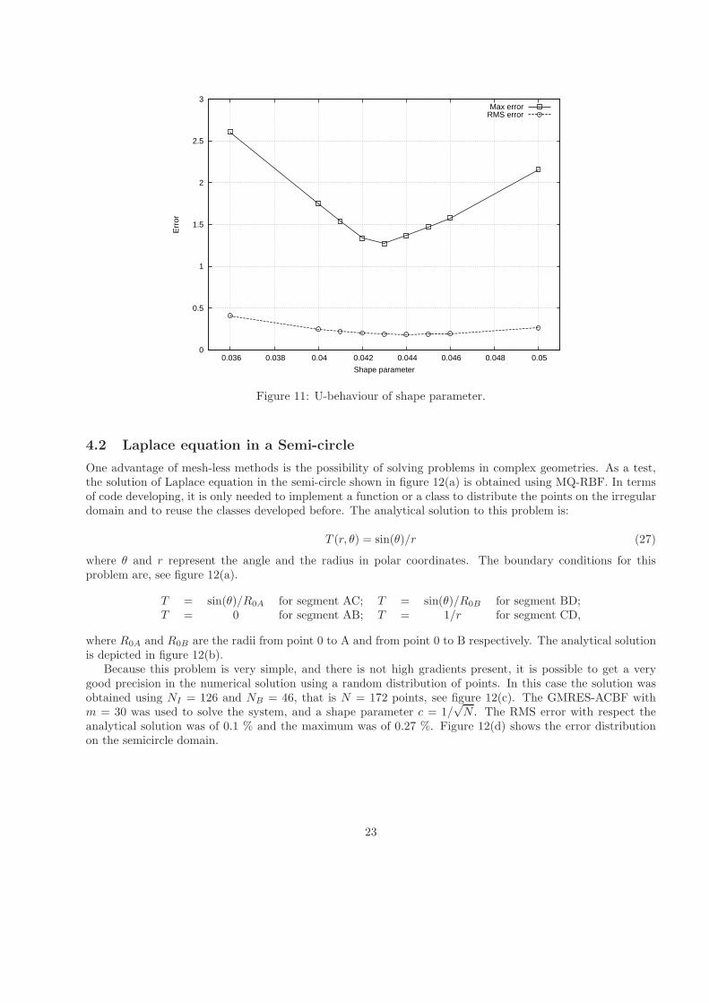
The MQ-RBF incorporate a user-defined shape parameter c. The value of this scalar determines the region ofinfluence of the MQ-RBF kernel. Many numerical studies using MQ-RBF have shown that this kernel givesbetter performance than others, and it has been observed that the accuracy of the numerical solutions dependsheavily on the value of c. An optimal value of this parameter is not easy to find and is still an open problem inthe literature. The influence of the shape parameter on the accuracy of the solution follows a U-shape curve.The figure 12 depicts the behaviour of the error in the case of the problem studied in the previous sections. Ascan be seen, a short value of c produce bad accuracy, a minimum of the error is reached when c ≈ 1/

√N , and

after this value the accuracy become worse as c is incremented. The value c = 1/√N has been used in several

studies with good results, see for example [19].

22

0

0.5

1

1.5

2

2.5

3

0.036 0.038 0.04 0.042 0.044 0.046 0.048 0.05

Err

or

Shape parameter

Max errorRMS error

Figure 11: U-behaviour of shape parameter.

4.2 Laplace equation in a Semi-circle

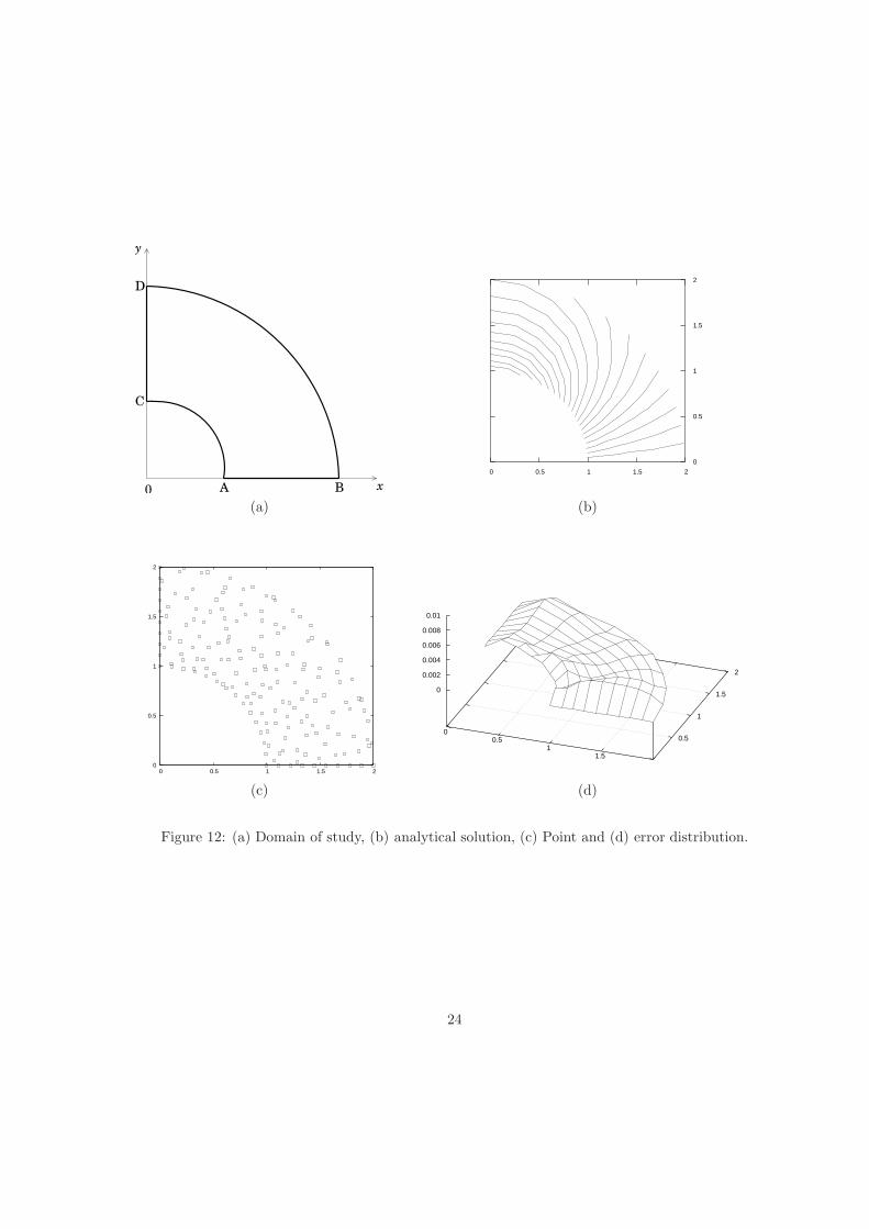
One advantage of mesh-less methods is the possibility of solving problems in complex geometries. As a test,the solution of Laplace equation in the semi-circle shown in figure 12(a) is obtained using MQ-RBF. In termsof code developing, it is only needed to implement a function or a class to distribute the points on the irregulardomain and to reuse the classes developed before. The analytical solution to this problem is:

T (r, θ) = sin(θ)/r (27)

where θ and r represent the angle and the radius in polar coordinates. The boundary conditions for thisproblem are, see figure 12(a).

T = sin(θ)/R0A for segment AC; T = sin(θ)/R0B for segment BD;T = 0 for segment AB; T = 1/r for segment CD,

where R0A and R0B are the radii from point 0 to A and from point 0 to B respectively. The analytical solutionis depicted in figure 12(b).

Because this problem is very simple, and there is not high gradients present, it is possible to get a verygood precision in the numerical solution using a random distribution of points. In this case the solution wasobtained using NI = 126 and NB = 46, that is N = 172 points, see figure 12(c). The GMRES-ACBF withm = 30 was used to solve the system, and a shape parameter c = 1/

√N . The RMS error with respect the

analytical solution was of 0.1 % and the maximum was of 0.27 %. Figure 12(d) shows the error distributionon the semicircle domain.

23

y

x0

C

D

A B

0 0.5 1 1.5 2

0

0.5

1

1.5

2

(a) (b)

0

0.5

1

1.5

2

0 0.5 1 1.5 2

0 0.5

1 1.5

0.5

1

1.5

2

0

0.002

0.004

0.006

0.008

0.01

(c) (d)

Figure 12: (a) Domain of study, (b) analytical solution, (c) Point and (d) error distribution.

24

4.3 Linear time-dependent advection-diffusion in 1D

The time-dependent advection-diffusion equation in one dimension is written as follows:

∂f

∂t+ u

∂f

∂x= Γ

∂2f

∂x2(28)

where x and t are the space and time coordinates respectively, Γ is the diffusion coefficient, u is a constantinput velocity. The initial and boundary conditions for this example are

f(x, 0) = 0, for 0 ≤ x ≤ ∞, (29)

f(0, t) = 1, for t > 0, (30)

f(L, t) = 0, for t > 0, L→∞. (31)

The exact solution of this moving front problem for Γ > 0 is

f(x, t) = 0.5

[

erfc

(

x− ut2√

Γt

)

+ exp(ux

D

)

erfc

(

x+ ut

2√

Γt

)]

(32)

where erfc is the complementary error function.To construct the solution in terms of RBF, the MQ kernel and its derivatives are assumed to be fixed and

the coefficients vary in time, that is λj = λj(t). Let fk ≈ f(x, k∆t). A backward Euler difference scheme isused to approximate the time derivative in equation (28):

∂f(x, t)

∂t≈ fk+1 − fk

∆t(33)

then, using (33) in (28) results in the next sequence:

fk+1 + ∆t

[

u∂fk+1

∂x− Γ

∂2fk+1

∂x2

]

= fk

Now, expanding the left-hand side of this equation using MQ-RBF the next linear system is obtained

N∑

j=1

λk+1j φj(ri) + ∆t

u

N∑

j=1

λk+1j

∂φj(ri)

∂x− Γ

N∑

j=1

λk+1j

∂2φj(ri)

∂x2

= fk, for 1 ≤ i ≤ NI , k = 0, 1, . . . (34)

where λk+1j represents the value of the coefficient λj at t = (k+1)∆t. Note that the solution at t = k∆t is used

as the initial guess for the matrix system defined at t = (k + 1)∆t. For the first step, the right-hand vector isgiven by the initial conditions (29). The system (34) is completed with the expansion of boundary conditions,equations (30) and (31) in terms of MQ-RBF, yielding an N ×N linear system.

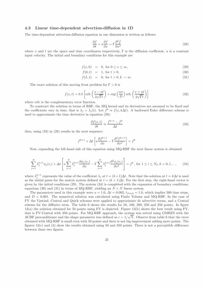
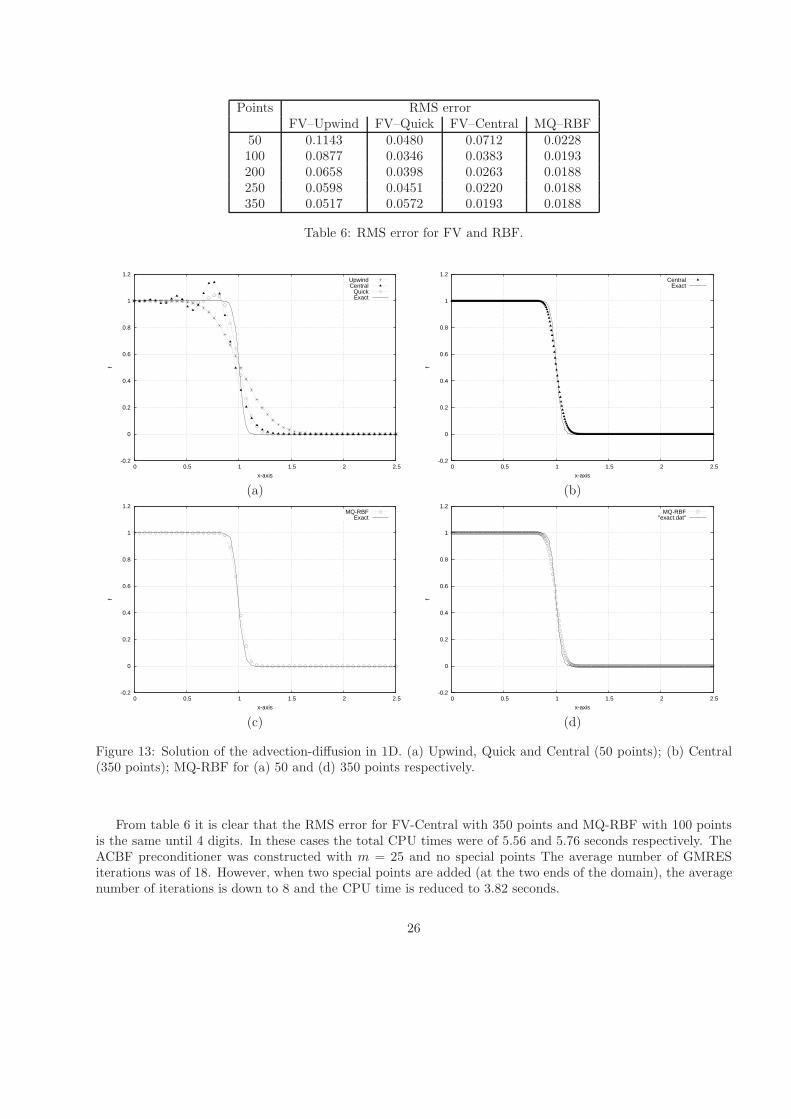
The parameters used in this example were u = 1.0, ∆t = 0.002, tfinal = 1.0, which implies 500 time steps,and D = 0.001. The numerical solution was calculated using Finite Volume and MQ-RBF. In the case ofFV the Upwind, Central and Quick schemes were applied to approximate de advective terms, and a Centralscheme for the diffusive term. The table 6 shows the results for 50, 100, 200, 250 and 350 points. In figure13(a) the solution obtained for 50 points using FV is depicted. Figure 13(b) shows the best result using FV,that is FV-Central with 350 points. For MQ-RBF approach, the system was solved using GMRES with theACBF preconditioner and the shape parameter was defined as c = 1/

√N . Observe from table 6 that the error

obtained with MQ-RBF is small even with 50 points and there is not big improvement adding more points. Thefigures 13(c) and (d) show the results obtained using 50 and 350 points. There is not a perceptible differencebetween these two figures.

25

Points RMS errorFV–Upwind FV–Quick FV–Central MQ–RBF

50 0.1143 0.0480 0.0712 0.0228100 0.0877 0.0346 0.0383 0.0193200 0.0658 0.0398 0.0263 0.0188250 0.0598 0.0451 0.0220 0.0188350 0.0517 0.0572 0.0193 0.0188

Table 6: RMS error for FV and RBF.

-0.2

0

0.2

0.4

0.6

0.8

1

1.2

0 0.5 1 1.5 2 2.5

f

x-axis

UpwindCentral

QuickExact

-0.2

0

0.2

0.4

0.6

0.8

1

1.2

0 0.5 1 1.5 2 2.5

f

x-axis

CentralExact

(a) (b)

-0.2

0

0.2

0.4

0.6

0.8

1

1.2

0 0.5 1 1.5 2 2.5

f

x-axis

MQ-RBFExact

-0.2

0

0.2

0.4

0.6

0.8

1

1.2

0 0.5 1 1.5 2 2.5

f

x-axis

MQ-RBF"exact.dat"

(c) (d)

Figure 13: Solution of the advection-diffusion in 1D. (a) Upwind, Quick and Central (50 points); (b) Central(350 points); MQ-RBF for (a) 50 and (d) 350 points respectively.

From table 6 it is clear that the RMS error for FV-Central with 350 points and MQ-RBF with 100 pointsis the same until 4 digits. In these cases the total CPU times were of 5.56 and 5.76 seconds respectively. TheACBF preconditioner was constructed with m = 25 and no special points The average number of GMRESiterations was of 18. However, when two special points are added (at the two ends of the domain), the averagenumber of iterations is down to 8 and the CPU time is reduced to 3.82 seconds.

26

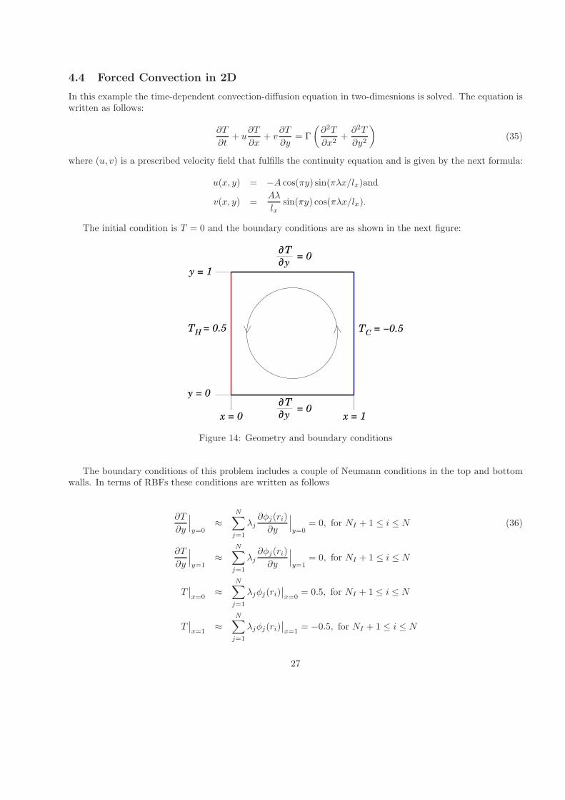
4.4 Forced Convection in 2D

In this example the time-dependent convection-diffusion equation in two-dimesnions is solved. The equation iswritten as follows:

∂T

∂t+ u

∂T

∂x+ v

∂T

∂y= Γ

(

∂2T

∂x2+∂2T

∂y2

)

(35)

where (u, v) is a prescribed velocity field that fulfills the continuity equation and is given by the next formula:

u(x, y) = −A cos(πy) sin(πλx/lx)and

v(x, y) =Aλ

lxsin(πy) cos(πλx/lx).

The initial condition is T = 0 and the boundary conditions are as shown in the next figure:

∂T

∂y= 0

HT = 0.5 T = −0.5C

∂T

∂y= 0

x = 0

y = 0

x = 1

y = 1

Figure 14: Geometry and boundary conditions

The boundary conditions of this problem includes a couple of Neumann conditions in the top and bottomwalls. In terms of RBFs these conditions are written as follows

∂T

∂y

∣

∣

∣

y=0≈

N∑

j=1

λj∂φj(ri)

∂y

∣

∣

∣

y=0= 0, for NI + 1 ≤ i ≤ N (36)

∂T

∂y

∣

∣

∣

y=1≈

N∑

j=1

λj∂φj(ri)

∂y

∣

∣

∣

y=1= 0, for NI + 1 ≤ i ≤ N

T∣

∣

x=0≈

N∑

j=1

λjφj(ri)∣

∣

x=0= 0.5, for NI + 1 ≤ i ≤ N

T∣

∣

x=1≈

N∑

j=1

λjφj(ri)∣

∣

x=1= −0.5, for NI + 1 ≤ i ≤ N

27

The equations (36) are incorporated in the global linear system as was described in section 2.3. The sameformulation for the temporal derivatives as in section 4.3 was used here. The final linear system is written asfollows

[

WL11 WL12

WB21 WB22

]k

Λ = ~T k (37)

where the indices k and k+ 1 represents values at t = k∆t and t = (k+ 1)∆t. The sub-matrices WL11, WL12,WB21 and WB22 are as defined in section 2.3 and the operators L and B are:

L = I + ∆t

[

u∂

∂x+ v

∂

∂y− Γ

(

∂2

∂2x+

∂2

∂2y

)]

B = I, for x = 0, 1

B =∂

∂y, for y = 0, 1

(38)

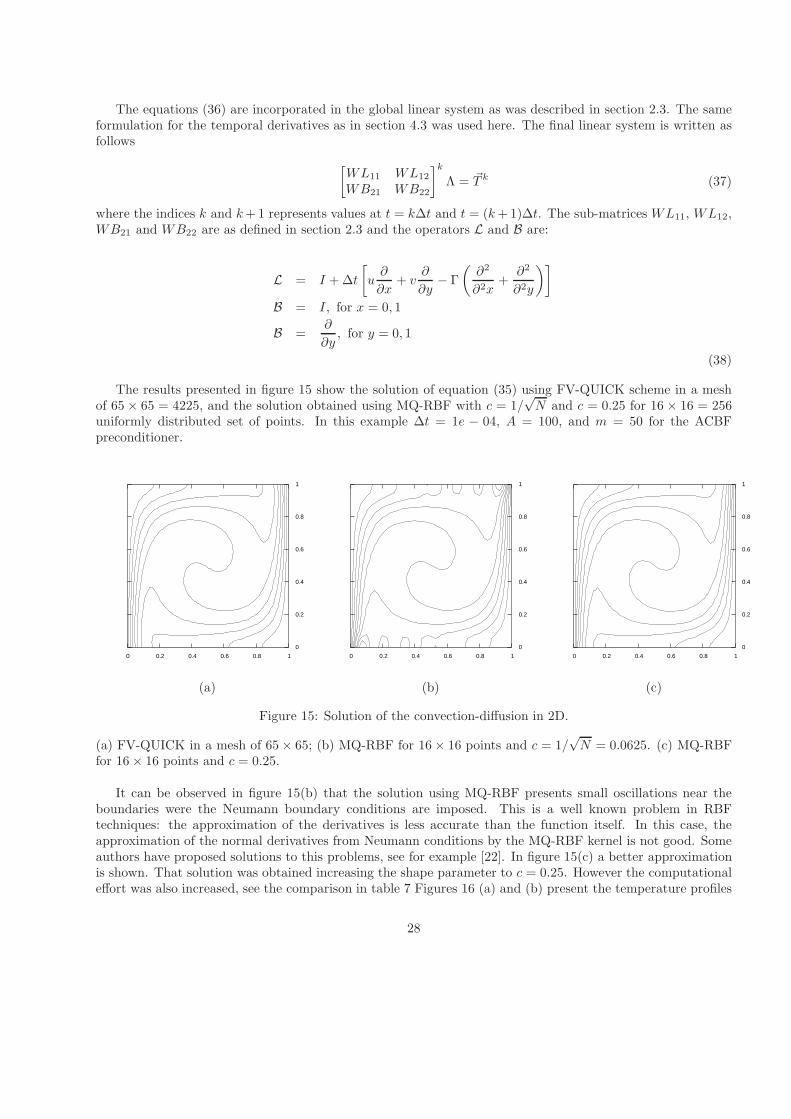
The results presented in figure 15 show the solution of equation (35) using FV-QUICK scheme in a meshof 65 × 65 = 4225, and the solution obtained using MQ-RBF with c = 1/

√N and c = 0.25 for 16 × 16 = 256

uniformly distributed set of points. In this example ∆t = 1e − 04, A = 100, and m = 50 for the ACBFpreconditioner.

0 0.2 0.4 0.6 0.8 1

0

0.2

0.4

0.6

0.8

1

0 0.2 0.4 0.6 0.8 1

0

0.2

0.4

0.6

0.8

1

0 0.2 0.4 0.6 0.8 1

0

0.2

0.4

0.6

0.8

1

(a) (b) (c)

Figure 15: Solution of the convection-diffusion in 2D.

(a) FV-QUICK in a mesh of 65× 65; (b) MQ-RBF for 16× 16 points and c = 1/√N = 0.0625. (c) MQ-RBF

for 16× 16 points and c = 0.25.

It can be observed in figure 15(b) that the solution using MQ-RBF presents small oscillations near theboundaries were the Neumann boundary conditions are imposed. This is a well known problem in RBFtechniques: the approximation of the derivatives is less accurate than the function itself. In this case, theapproximation of the normal derivatives from Neumann conditions by the MQ-RBF kernel is not good. Someauthors have proposed solutions to this problems, see for example [22]. In figure 15(c) a better approximationis shown. That solution was obtained increasing the shape parameter to c = 0.25. However the computationaleffort was also increased, see the comparison in table 7 Figures 16 (a) and (b) present the temperature profiles

28

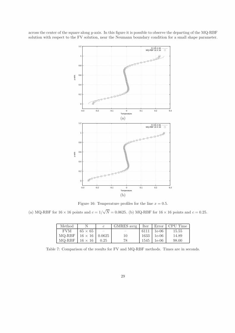
across the center of the square along y-axis. In this figure it is possible to observe the departing of the MQ-RBFsolution with respect to the FV solution, near the Neumann boundary condition for a small shape parameter.

0

0.2

0.4

0.6

0.8

1

1.2

-0.3 -0.2 -0.1 0 0.1 0.2 0.3

y-ax

is

Temperature

FV 65 X 65MQ-RBF 16 X 16

(a)

0

0.2

0.4

0.6

0.8

1

1.2

-0.3 -0.2 -0.1 0 0.1 0.2 0.3

y-ax

is

Temperature

FV 65 X 65MQ-RBF 16 X 16

(b)

Figure 16: Temperature profiles for the line x = 0.5.

(a) MQ-RBF for 16× 16 points and c = 1/√N = 0.0625. (b) MQ-RBF for 16× 16 points and c = 0.25.

Method N c GMRES avrg Iter Error CPU TimeFVM 65 × 65 – – 6111 1e-06 15.55

MQ-RBF 16 × 16 0.0625 10 1633 1e-06 14.89MQ-RBF 16 × 16 0.25 78 1545 1e-06 98.00

Table 7: Comparison of the results for FV and MQ-RBF methods. Times are in seconds.

29

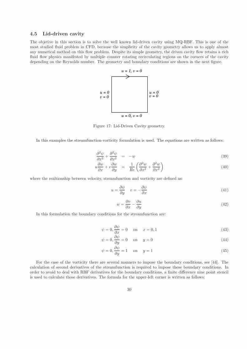
4.5 Lid-driven cavity

The objetive in this section is to solve the well known lid-driven cavity using MQ-RBF. This is one of themost studied fluid problem in CFD, because the simplicity of the cavity geometry allows us to apply almostany numerical method on this flow problem. Despite its simple geometry, the driven cavity flow retains a richfluid flow physics manifested by multiple counter rotating recirculating regions on the corners of the cavitydepending on the Reynolds number. The geometry and boundary conditions are shown in the next figure.

u = 1, v = 0

v = 0u = 0 u = 0

v = 0

u = 0, v = 0

Figure 17: Lid-Driven Cavity geometry.

In this examples the streamfunction-vorticity formulation is used. The equations are written as follows:

∂2ψ

∂x2+∂2ψ

∂x2= −w (39)

u∂w

∂x+ v

∂w

∂y=

1

Re

(

∂2w

∂x2+∂2w

∂x2

)

(40)

where the realtionship between velocity, streamfunction and vorticity are defined as:

u =∂ψ

∂yv = −∂ψ

∂x(41)

w =∂v

∂x− ∂u

∂y(42)

In this formulation the boundary conditions for the streamfunction are:

ψ = 0,∂ψ

∂x= 0 on x = 0, 1 (43)

ψ = 0,∂ψ

∂y= 0 on y = 0 (44)

ψ = 0,∂ψ

∂y= 1 on y = 1 (45)

For the case of the vorticity there are several manners to impose the boundary conditions, see [44]. Thecalculation of second derivatives of the streamfunction is required to impose these boundary conditions. Inorder to avoid to deal with RBF derivatives for the boundary conditions, a finite difference nine point stencilis used to calculate those derivatives. The formula for the upper-left corner is written as follows:

30

1

3h2

• • •• −2 1

2• 1

2 1

ψh +1

9

• • •• 1 1

2• 1

214

wh = − 1

2h(46)

and for the top wall the formula is:

1

3h2

• • •12 −4 1

21 1 1

ψh +1

9

• • •12 2 1

214 1 1

4

wh = − 1

h(47)

In the above formula a •means a point on the boundary. For other corners and walls the formulae aresimilar.

As we can observe, the equations (39) and (40) are strongly coupled by the convective terms. In order todeal with this non-linear coupling the next pseudo-temporal formulation is used:

∂ψ

∂τ−

∂2ψ

∂x2+∂2ψ

∂y2+ w

= 0 (48)

∂w

∂τ−

∂2w

∂x2+∂2w

∂y2−Re

(

u∂w

∂x+ v

∂w

∂y

)

= 0 (49)

Substituing the RBF formulation for w and ψ, as was seen in section 2.3, and applying a backward Eulerscheme for the pseudo-temporal derivatives the above equations are converted in the next two linear systems:

N∑

j=1

[λψ ]kj

[

φkij −∆τ

∂2φkij∂x2

+∂2φkij∂y2

]

= φk−1ij + wk∆τ (50)

N∑

j=1

[λw ]kj

[

φkij −∆τ

∂2φkij∂x2

+∂2φkij∂y2

−Re(

u∂φkij∂x

+ v∂φkij∂y

)]

= φk−1ij (51)

where [λw]kj and [λψ ]kj are the unknown cofficients for the MQ-RBF formulation of the vorticity and thestreamfunction respectively; the superscript k means the value of a variable at the k-th iteration; φij = φj(ri);i, j = 1, . . .N ; ∆τ is the pseudo-time step.

The velocity components are calculated via the first derivatives of the streamfunction. These derivativescan be calculated using the RBF kernel as follows:

ui =∂ψi∂y

=

N∑

j=1

[λψ ]j∂φij∂y

(52)

vi = −∂ψi∂x

= −N∑

j=1

[λψ ]j∂φij∂x

(53)

The algorithm used to solve the coupled equations of this problem is as follows:

31

RBf algorithm to solve the Lid-driven cavity problem

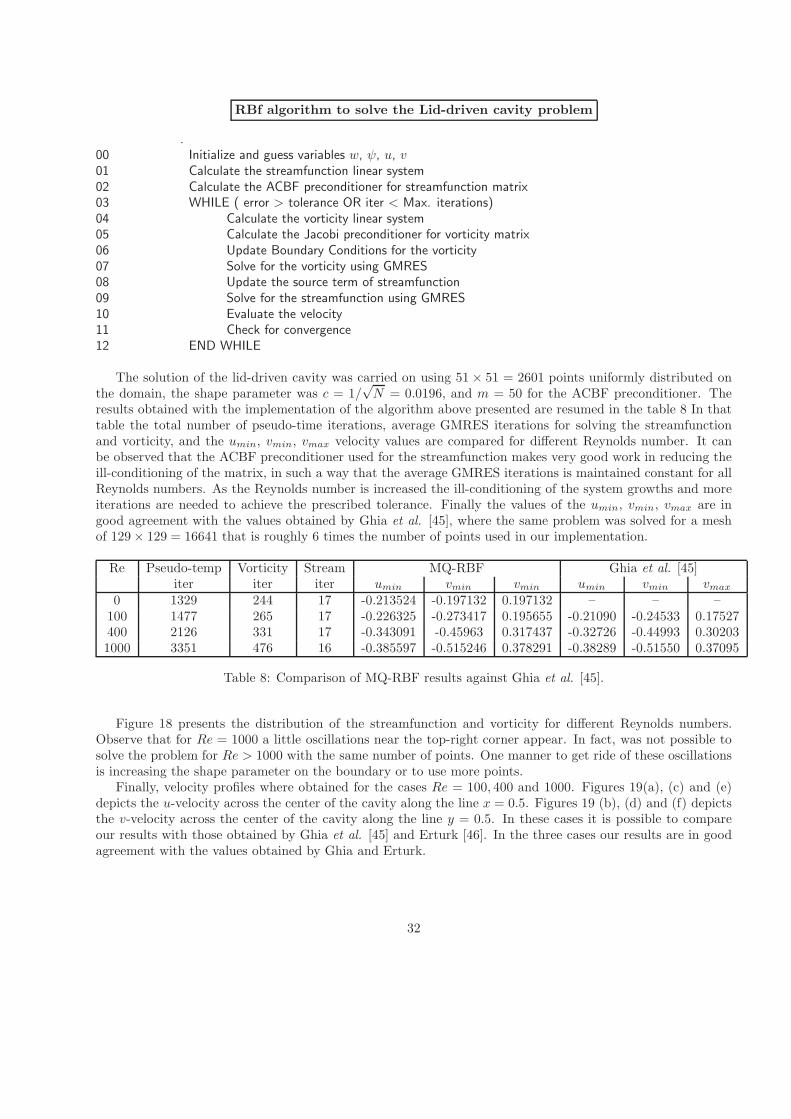
.00 Initialize and guess variables w, ψ, u, v01 Calculate the streamfunction linear system02 Calculate the ACBF preconditioner for streamfunction matrix03 WHILE ( error > tolerance OR iter < Max. iterations)04 Calculate the vorticity linear system05 Calculate the Jacobi preconditioner for vorticity matrix06 Update Boundary Conditions for the vorticity07 Solve for the vorticity using GMRES08 Update the source term of streamfunction09 Solve for the streamfunction using GMRES10 Evaluate the velocity11 Check for convergence12 END WHILE

The solution of the lid-driven cavity was carried on using 51× 51 = 2601 points uniformly distributed onthe domain, the shape parameter was c = 1/

√N = 0.0196, and m = 50 for the ACBF preconditioner. The

results obtained with the implementation of the algorithm above presented are resumed in the table 8 In thattable the total number of pseudo-time iterations, average GMRES iterations for solving the streamfunctionand vorticity, and the umin, vmin, vmax velocity values are compared for different Reynolds number. It canbe observed that the ACBF preconditioner used for the streamfunction makes very good work in reducing theill-conditioning of the matrix, in such a way that the average GMRES iterations is maintained constant for allReynolds numbers. As the Reynolds number is increased the ill-conditioning of the system growths and moreiterations are needed to achieve the prescribed tolerance. Finally the values of the umin, vmin, vmax are ingood agreement with the values obtained by Ghia et al. [45], where the same problem was solved for a meshof 129× 129 = 16641 that is roughly 6 times the number of points used in our implementation.

Re Pseudo-temp Vorticity Stream MQ-RBF Ghia et al. [45]iter iter iter umin vmin vmin umin vmin vmax

0 1329 244 17 -0.213524 -0.197132 0.197132 – – –100 1477 265 17 -0.226325 -0.273417 0.195655 -0.21090 -0.24533 0.17527400 2126 331 17 -0.343091 -0.45963 0.317437 -0.32726 -0.44993 0.302031000 3351 476 16 -0.385597 -0.515246 0.378291 -0.38289 -0.51550 0.37095

Table 8: Comparison of MQ-RBF results against Ghia et al. [45].

Figure 18 presents the distribution of the streamfunction and vorticity for different Reynolds numbers.Observe that for Re = 1000 a little oscillations near the top-right corner appear. In fact, was not possible tosolve the problem for Re > 1000 with the same number of points. One manner to get ride of these oscillationsis increasing the shape parameter on the boundary or to use more points.

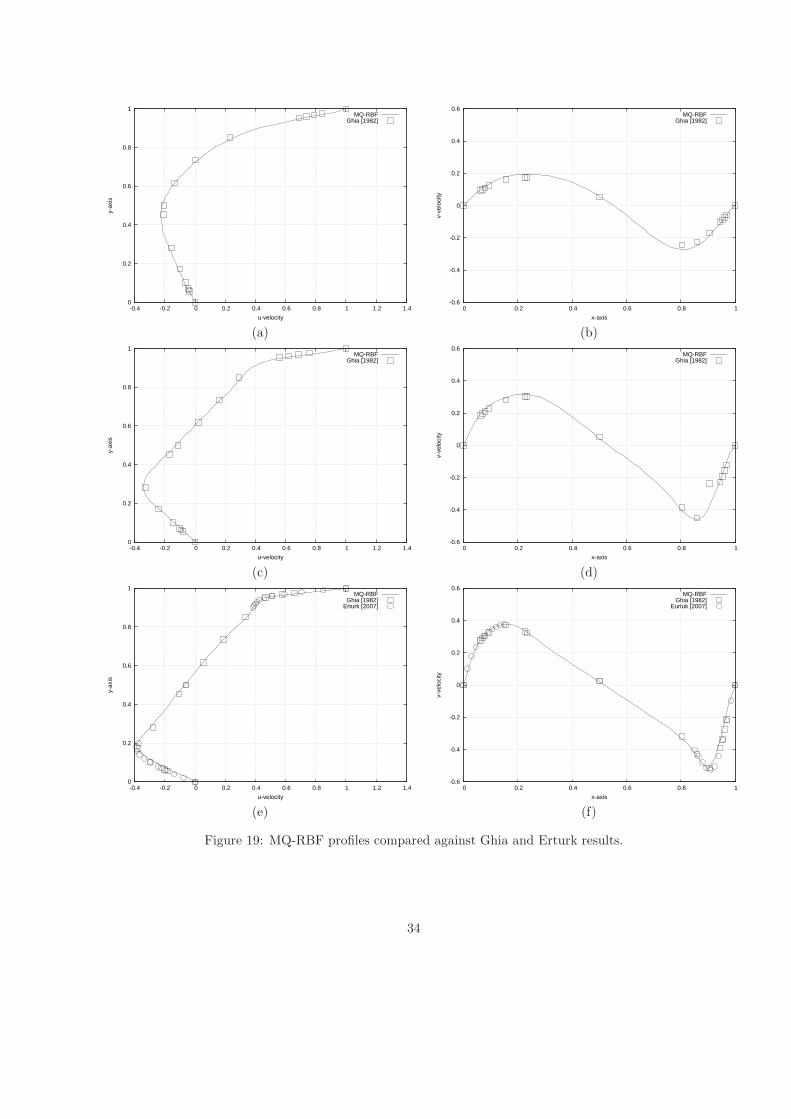
Finally, velocity profiles where obtained for the cases Re = 100, 400 and 1000. Figures 19(a), (c) and (e)depicts the u-velocity across the center of the cavity along the line x = 0.5. Figures 19 (b), (d) and (f) depictsthe v-velocity across the center of the cavity along the line y = 0.5. In these cases it is possible to compareour results with those obtained by Ghia et al. [45] and Erturk [46]. In the three cases our results are in goodagreement with the values obtained by Ghia and Erturk.

32

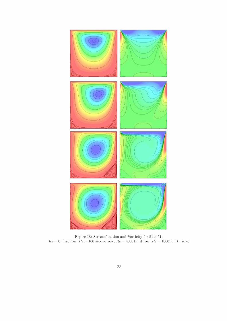
Figure 18: Streamfunction and Vorticity for 51× 51.Re = 0, first row; Re = 100 second row; Re = 400, third row; Re = 1000 fourth row;

33

0

0.2

0.4

0.6

0.8

1

-0.4 -0.2 0 0.2 0.4 0.6 0.8 1 1.2 1.4

y-ax

is

u-velocity

MQ-RBFGhia [1982]

-0.6

-0.4

-0.2

0

0.2

0.4

0.6

0 0.2 0.4 0.6 0.8 1

v-ve

loci

ty

x-axis

MQ-RBFGhia [1982]

(a) (b)

0

0.2

0.4

0.6

0.8

1

-0.4 -0.2 0 0.2 0.4 0.6 0.8 1 1.2 1.4

y-ax

is

u-velocity

MQ-RBFGhia [1982]

-0.6

-0.4

-0.2

0

0.2

0.4

0.6

0 0.2 0.4 0.6 0.8 1

v-ve

loci

ty

x-axis

MQ-RBFGhia [1982]

(c) (d)

0

0.2

0.4

0.6

0.8

1

-0.4 -0.2 0 0.2 0.4 0.6 0.8 1 1.2 1.4

y-ax

is

u-velocity

MQ-RBFGhia [1982]

Erturk [2007]

-0.6

-0.4

-0.2

0

0.2

0.4

0.6

0 0.2 0.4 0.6 0.8 1

v-ve

loci

ty

x-axis

MQ-RBFGhia [1982]

Eurtuk [2007]

(e) (f)

Figure 19: MQ-RBF profiles compared against Ghia and Erturk results.

34

4.6 Backward-facing step

Fluid flows in channels with flow separation and reattachment of the boundary layers are encountered inmany flow problems. Typical examples are the flows in heat exchangers and ducts. Among this type of flowproblems, a backward-facing step can be regarded as having the simplest geometry while retaining rich flowphysics manifested by flow separation, flow reattachment and multiple recirculating bubbles in the channeldepending on the Reynolds number and the geometrical parameters such as the step height and the channellength.

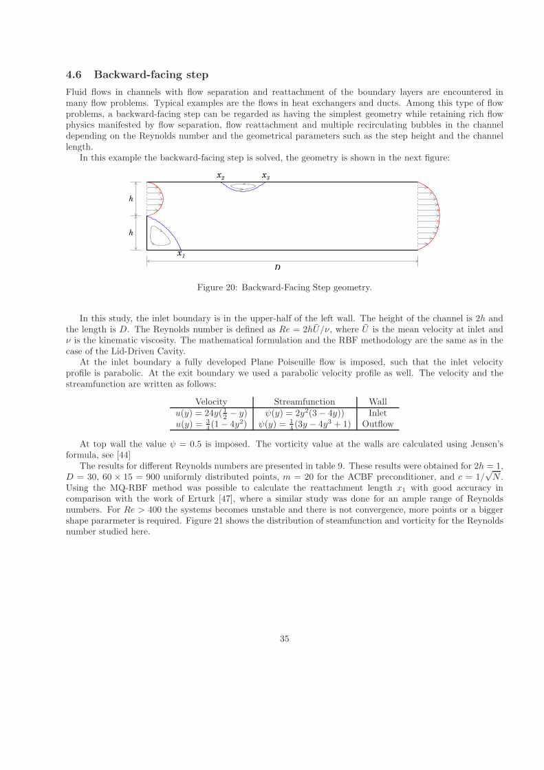
In this example the backward-facing step is solved, the geometry is shown in the next figure:

h

h

2x 3x

1x

D

Figure 20: Backward-Facing Step geometry.

In this study, the inlet boundary is in the upper-half of the left wall. The height of the channel is 2h andthe length is D. The Reynolds number is defined as Re = 2hU/ν, where U is the mean velocity at inlet andν is the kinematic viscosity. The mathematical formulation and the RBF methodology are the same as in thecase of the Lid-Driven Cavity.

At the inlet boundary a fully developed Plane Poiseuille flow is imposed, such that the inlet velocityprofile is parabolic. At the exit boundary we used a parabolic velocity profile as well. The velocity and thestreamfunction are written as follows:

Velocity Streamfunction Wallu(y) = 24y(1

2 − y) ψ(y) = 2y2(3− 4y)) Inletu(y) = 3

4 (1− 4y2) ψ(y) = 14 (3y − 4y3 + 1) Outflow

At top wall the value ψ = 0.5 is imposed. The vorticity value at the walls are calculated using Jensen’sformula, see [44]

The results for different Reynolds numbers are presented in table 9. These results were obtained for 2h = 1,D = 30, 60 × 15 = 900 uniformly distributed points, m = 20 for the ACBF preconditioner, and c = 1/

√N .

Using the MQ-RBF method was possible to calculate the reattachment length x1 with good accuracy incomparison with the work of Erturk [47], where a similar study was done for an ample range of Reynoldsnumbers. For Re > 400 the systems becomes unstable and there is not convergence, more points or a biggershape pararmeter is required. Figure 21 shows the distribution of steamfunction and vorticity for the Reynoldsnumber studied here.

35

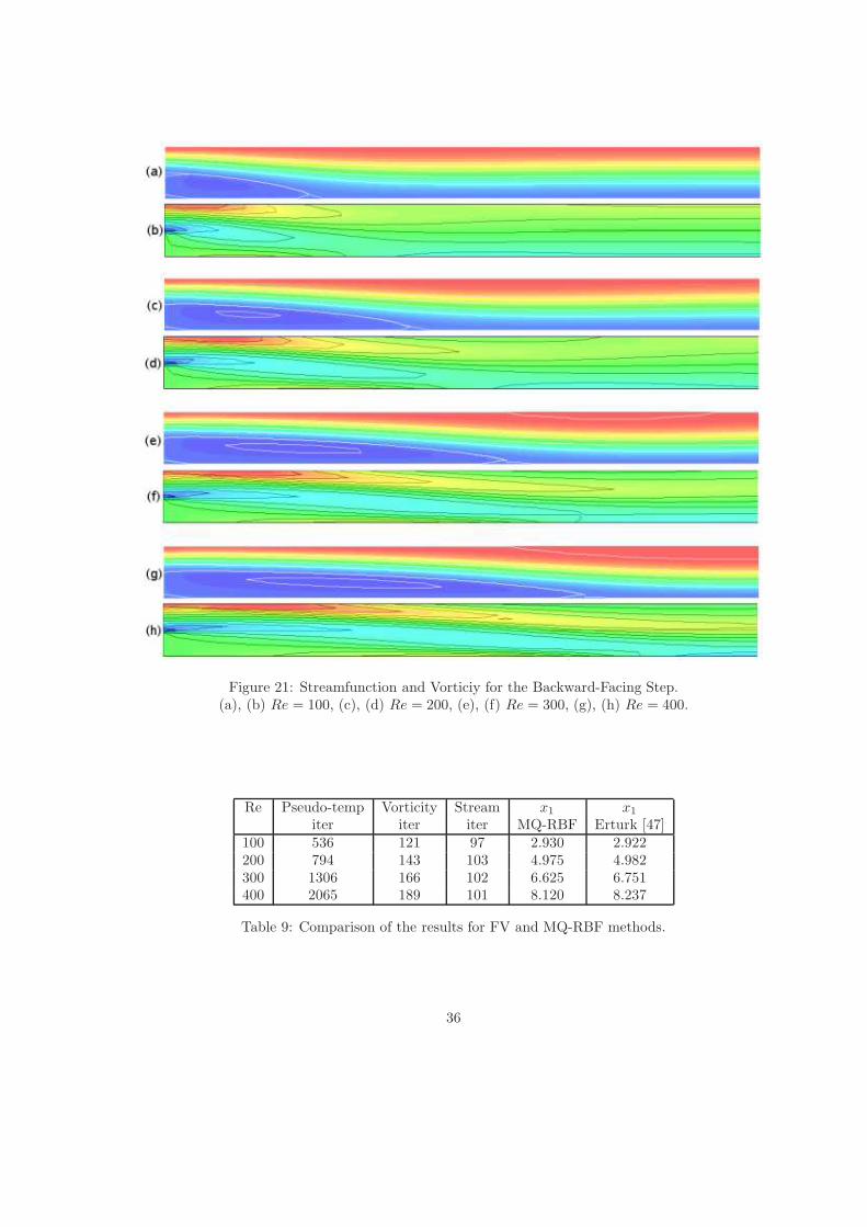
Figure 21: Streamfunction and Vorticiy for the Backward-Facing Step.(a), (b) Re = 100, (c), (d) Re = 200, (e), (f) Re = 300, (g), (h) Re = 400.

Re Pseudo-temp Vorticity Stream x1 x1

iter iter iter MQ-RBF Erturk [47]100 536 121 97 2.930 2.922200 794 143 103 4.975 4.982300 1306 166 102 6.625 6.751400 2065 189 101 8.120 8.237

Table 9: Comparison of the results for FV and MQ-RBF methods.

36

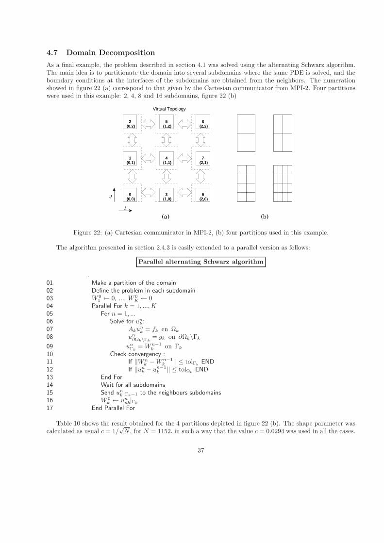
4.7 Domain Decomposition

As a final example, the problem described in section 4.1 was solved using the alternating Schwarz algorithm.The main idea is to partitionate the domain into several subdomains where the same PDE is solved, and theboundary conditions at the interfaces of the subdomains are obtained from the neighbors. The numerationshowed in figure 22 (a) correspond to that given by the Cartesian communicator from MPI-2. Four partitionswere used in this example: 2, 4, 8 and 16 subdomains, figure 22 (b)

(b)

(0,2)2

(1,2)5

(2,2)8

(2,1)7

(2,0)6

(1,0)3

(0,0)0

(0,1)1

(1,1)4

J

I

Virtual Topology

(a)

Figure 22: (a) Cartesian communicator in MPI-2, (b) four partitions used in this example.

The algorithm presented in section 2.4.3 is easily extended to a parallel version as follows:

Parallel alternating Schwarz algorithm

.01 Make a partition of the domain02 Define the problem in each subdomain03 W 0

1 ← 0, ..., W 0K ← 0

04 Parallel For k = 1, ...,K05 For n = 1, ...06 Solve for unk :07 Aku

nk = fk en Ωk

08 un∂Ωk\Γk= gk on ∂Ωk\Γk

09 unΓk= Wn−1

k on Γk10 Check convergency :11 If ||Wn

k −Wn−1k || ≤ tolΓk

END12 If ||unk − un−1

k || ≤ tolΩkEND

13 End For14 Wait for all subdomains15 Send unk |Γk−1 to the neighbours subdomains16 W 0

k ← unnb|Γk

17 End Parallel For

Table 10 shows the result obtained for the 4 partitions depicted in figure 22 (b). The shape parameter wascalculated as usual c = 1/

√N , for N = 1152, in such a way that the value c = 0.0294 was used in all the cases.

37

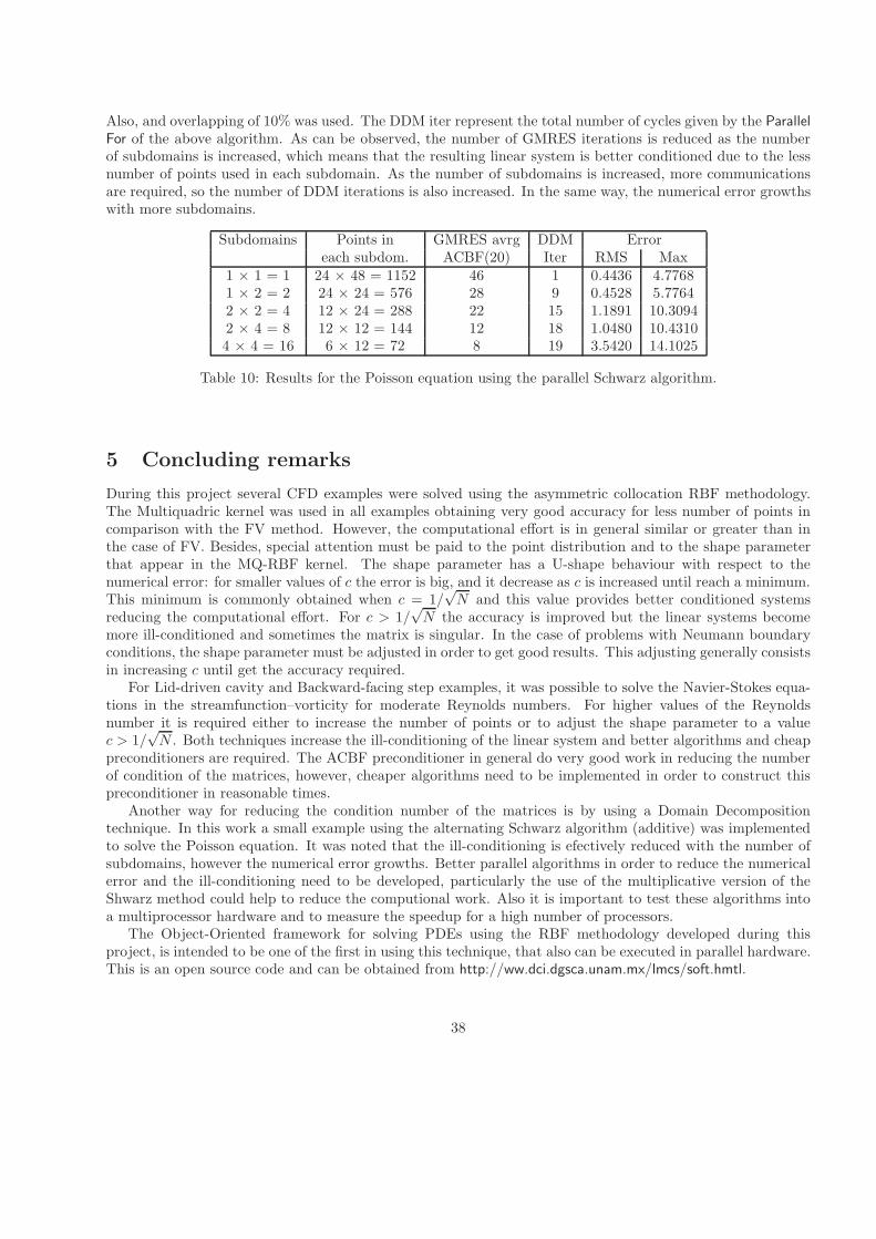
Also, and overlapping of 10% was used. The DDM iter represent the total number of cycles given by the ParallelFor of the above algorithm. As can be observed, the number of GMRES iterations is reduced as the numberof subdomains is increased, which means that the resulting linear system is better conditioned due to the lessnumber of points used in each subdomain. As the number of subdomains is increased, more communicationsare required, so the number of DDM iterations is also increased. In the same way, the numerical error growthswith more subdomains.

Subdomains Points in GMRES avrg DDM Erroreach subdom. ACBF(20) Iter RMS Max

1 × 1 = 1 24 × 48 = 1152 46 1 0.4436 4.77681 × 2 = 2 24 × 24 = 576 28 9 0.4528 5.77642 × 2 = 4 12 × 24 = 288 22 15 1.1891 10.30942 × 4 = 8 12 × 12 = 144 12 18 1.0480 10.43104 × 4 = 16 6 × 12 = 72 8 19 3.5420 14.1025

Table 10: Results for the Poisson equation using the parallel Schwarz algorithm.

5 Concluding remarks

During this project several CFD examples were solved using the asymmetric collocation RBF methodology.The Multiquadric kernel was used in all examples obtaining very good accuracy for less number of points incomparison with the FV method. However, the computational effort is in general similar or greater than inthe case of FV. Besides, special attention must be paid to the point distribution and to the shape parameterthat appear in the MQ-RBF kernel. The shape parameter has a U-shape behaviour with respect to thenumerical error: for smaller values of c the error is big, and it decrease as c is increased until reach a minimum.This minimum is commonly obtained when c = 1/

√N and this value provides better conditioned systems

reducing the computational effort. For c > 1/√N the accuracy is improved but the linear systems become

more ill-conditioned and sometimes the matrix is singular. In the case of problems with Neumann boundaryconditions, the shape parameter must be adjusted in order to get good results. This adjusting generally consistsin increasing c until get the accuracy required.

For Lid-driven cavity and Backward-facing step examples, it was possible to solve the Navier-Stokes equa-tions in the streamfunction–vorticity for moderate Reynolds numbers. For higher values of the Reynoldsnumber it is required either to increase the number of points or to adjust the shape parameter to a valuec > 1/

√N . Both techniques increase the ill-conditioning of the linear system and better algorithms and cheap

preconditioners are required. The ACBF preconditioner in general do very good work in reducing the numberof condition of the matrices, however, cheaper algorithms need to be implemented in order to construct thispreconditioner in reasonable times.

Another way for reducing the condition number of the matrices is by using a Domain Decompositiontechnique. In this work a small example using the alternating Schwarz algorithm (additive) was implementedto solve the Poisson equation. It was noted that the ill-conditioning is efectively reduced with the number ofsubdomains, however the numerical error growths. Better parallel algorithms in order to reduce the numericalerror and the ill-conditioning need to be developed, particularly the use of the multiplicative version of theShwarz method could help to reduce the computional work. Also it is important to test these algorithms intoa multiprocessor hardware and to measure the speedup for a high number of processors.

The Object-Oriented framework for solving PDEs using the RBF methodology developed during thisproject, is intended to be one of the first in using this technique, that also can be executed in parallel hardware.This is an open source code and can be obtained from http://ww.dci.dgsca.unam.mx/lmcs/soft.hmtl.

38

References

[1] T Belytschko, Y Y Lu, L Gu, and P Krysl. Element-free galerkin methods. International Journal of

Numerical Methods in Engineering.

[2] T Belytschko, Y Krongauze, D Organ, M Fleming, and P Krysl. Meshless methods: an overview andrecent developments. Computational Methods Appl. M.

[3] I Babuska, U Banerjee, and J E Osborn. Survey of meshless and generalized finite element methods: aunified approach. Acta Numerica.

[4] Edward J. Kansa. Multiquadrics–a scattered data approximation scheme with applications to compu-tational fluid-dynamics–i. surface approximations and partial derivatives estimates. Computers Math.

Applic., 19(8/9):127–145, 1990.

[5] Edward J. Kansa. Multiquadrics–a scattered data approximation scheme with applications to compu-tational fluid-dynamics–ii. solutions to parabolic, hyperbolic and elliptic partial differential equations.Computers Math. Applic., 19(8/9):147–161, 1990.

[6] Martin D. Buhmann and M. D. Buhmann. Radial Basis Functions. Cambridge University Press, NewYork, NY, USA, 2003.

[7] R Franke. Scattered data interpolation: Tests of some methods. Math. Comp., 38(157):292–300, 1982.

[8] R L Hardy. Multiquadric equations of topography and other irregular surfaces. J. Geophys. Res., 176:1905–1915, 1971.

[9] R L Hardy. Theory and applications of the multiquadric-biharmonic method. 20 years of discovery19681988. Computers Math. Applic., 10(8/9):163–208, 1990.

[10] W R Madych and S A Nelson. Nelson, multivariate interpolation and conditionally positive definitefunctions. Approx. Theory Appl.

[11] A.I Fedoseyev, M.J Friedman, and E J Kansa. Improved multiquadric method for elliptic partial differentialequations via pde collocation on the boundary. An International Journal Computers & Mathematics with

Applications, 43:439–455, Feb 2002.

[12] B.J.C Baxter. Preconditioned conjugate gradients, radial basis functions, and toeplitz matrices. An

International Journal Computers & Mathematics with Applications, 43:305–318, Feb 2002.

[13] R K Beatson and G N Newsam. Fast evaluation of radial basis functions: Moment-based methods. SIAM

Journal of Scientific Computing, 19(5):1428–1449, Apr 1998.

[14] R K Beatson, J B Cherrie, and C T Mouat. Fast fitting of radial basis functions: Methods based onpreconditioned gmres iteration. Advances in Computational Mathematics, 11:253–270, Oct 1999.

[15] R K Beatson, W A Light, and S Billings. Fast solution of the radial basis function interpolation equations:Domain decomposition methods. SIAM Journal of Scientific Computing, 22(5):1717–1740, Dec 2000.

[16] E J Kansa and Y C Hon. Circumventing the ill-conditioning problem with multiquadric radial basisfunctions: Applications to elliptic partial differential equations. An International Journal Computers &

Mathematics with Applications, 39:123–137, Jan 2000.

[17] X Zhou, Y C Hon, and Jichun Li. Overlapping domain decomposition method by radial basis functions.Applied Numerical Mathematics, 44:241–255, Dec 2003.

39

[18] Leevan Ling and E J Kansa. Preconditioning for radial basis functions with domain decomposition meth-ods. Mathematical and Computer Modelling, 40:1413–1427, Jan 2004.

[19] Leevan Ling and E J Kansa. A least-squares preconditioner for radial basis functions collocation methods.Advances in Computational Mathematics, 23:31–54, Mar 2005.

[20] G. Fasshauer and J. Jerome. Multistep approximations algorithms: Improved convergence rates throughpostconditioning with smooting kernels. Adv. Comp. Math., 10:1–27, 1999.

[21] Damian Brown, Leevan Ling, E J Kansa, and Jermy Levesley. On approximate cardinal preconditioningmethods for solving pdes with radial basis functions. Engineering Analysis with Boundary Elements,29:343–353, Apr 2005.

[22] Nicolas Ali Libre, Arezoo Emdadi, E J Kansa, Mohammad Rahimian, and Mohammad Shekarchi. Astabilized rbf collocation scheme for neumann type boundary value problems. Computer Modelling in

Engineering & Sciences, 24(1):61–80, Feb 2008.

[23] Craig Larman. Applying UML and patterns: an introduction to object-oriented analysis and design. 1998.

[24] I. Jacobson, G. Booch, and J. Rumbaugh. The Unified Software Development Process. 1999.

[25] W Haerdle and M G Schimek, editors. Smoothing by local regression: principles and methods, StatisticalTheory and Comutational Aspects of Smoothing. Springer, 1996.

[26] H Wendland. Meshless galerkin methods using radial basis functions. Math. Comp., 68:1521–1531, 1999.

[27] C Franke and R Schaback. Convergence orders of meshless collocation methods using radial basis functions.Advances in Comp. Math., 8:381–399, 1998.

[28] C Franke and R Schaback. Solving partial differential equations by collocation using radial basis functions.Appl. Math. Comp., 93:73–82, 1998.

[29] G E Fasshauer. Solving differential equations with radial basis functions: multilevel methods and smooth-ing. Advances in Comp. Math., 11:139–159, 1999.

[30] L.R. Hardy. Theory and applications of the multiquadric-biharmonic method: 20 years of discovery.Computers Math. Applic., 19:163–208, 1990.

[31] M.J.D. Powell. The theory of radial basis function approximation in 1990. In Advances in Numerical

Analysis, Vol II. Oxford Science Publications, Oxford, 1992.

[32] Y Saad and M H Schultz. Gmres: a generalized minimal residual algorithm for solving nonsymmetriclinear equations. SIAM J. Sci. Statist. Comput.

[33] F P Preparata and M I Shamos. Computational Geometry: An introduction. Springer-Verlag, 1985.

[34] B. F. Smith, P. E. Bjorstad, and W. D. Gropp. Domain Decomposition: Parallel Multilevel Methods for

Elliptic Partial Differential Equations. Cambridge University Press, 1996.

[35] A S M Wong, Y C Hon, T S Li, S L Chung, and E J Kansa. Multizone decomposition for simulation of time-dependent problems using the multiquadric scheme. An International Journal Computers & Mathematics

with Applications, 37:23–43, Feb 1999.

[36] D. Vandevoorde and N. M. JosuttisOB. C++ Templates. 2003.

[37] Todd Veldhuizen. Using C++ template metaprograms. C++ Report, 7(4):36–43, May 1995. Reprinted inC++ Gems, ed. Stanley Lippman.

40

[38] Todd L. Veldhuizen. Expression templates. C++ Report, 7(5):26–31, June 1995. Reprinted in C++ Gems,ed. Stanley Lippman.

[39] The object-oriented numerics page. http://www.oonumerics.org.

[40] K. A. Hoffman. Computational Fluid Dynamics for Engineers. The University of Texas at Austin, 1989.

[41] S. V. Patankar. Numerical Heat Transfer and Fluid Flow. 1980.

[42] H.K. Versteeg and W. Malalasekera. An introduction to computational fluid dynamics: The finite volume

method. Longman, 1995.

[43] Template units for numerical application: The finite volume method.http://www.dci.dgsca.unam.mx/lmcs/soft.html.

[44] C. Fletcher. Computational Techniques for Fluid Dynamics 1: Specific Techniques for Different Flow

Categories. Springer–Verlag, second edition edition, 1991.

[45] U Ghia, K N Ghia, and C T Shin. High-re solutions for incompressible flow using the navier-stokesequations and a multigrid method. Journal of Computational Physics, 48:387–411, Dec 1982.

[46] Ercan Erturk, T C Corke, and C Gokcol. Numerical solutions of 2-d steady incompressible driven cavity.International Journal for Numerical Methods in Fluids, 48:747–774, Mar 2005.

[47] Ercan Erturk. Numerical solutions of 2-d steady incompressible flow over a backward-facing step, part i:High reynodls number solutions. Computers & Fluids, 37:633–655, 2008.

41