Scarring versus Selective Mortality: The long-term

effects of early life exposure to natural disasters in the

Philippines

⇤

Margaret Triyana

†and Xing Xia

‡

December 8, 2017

Preliminary Draft. Please Do Not Circulate or Cite without Permission

Abstract

This paper analyzes the long-term effects of early life shocks with varying degrees ofseverity on mortality and human capital outcomes in the Philippines. We exploit vari-ations in the geographical path and intensity of typhoons, as well as the introduction ofdisaster relief policies under Ferdinand Marcos to disentangle the effects of culling andscarring. Before Marcos, in-utero exposure to severe typhoons led to higher mortality;the average survivor exhibited similar levels of human capital as the unaffected. UnderMarcos, in-utero exposure to severe typhoons had little impact on mortality but signif-icantly reduced survivors’ educational attainment and occupational skill level. Theseadverse effects are intensified within families and among those born to disadvantagedparents.

Keywords: fetal origins hypothesis, selective mortality, Philippines, natural disas-ters, long term outcomes

JEL codes: I12, I15, O15⇤We are grateful to Julien Labonne, Douglas Almond, Bhashkar Mazumder, John Ham, Jessica Pan, Joe

Kaboski, seminar participants at Yale-NUS, NUS, University of Notre Dame, and participants of the 2017Conference on Health and Development for comments and suggestions. Michelle Quak provided invaluableassistance with GIS. Jason Carlo Carranceja and Adila Sayyed provided excellent research assistance. Thisresearch was financially supported by Yale-NUS College Start-up Grant, NUS HSS Seed Fund, and NanyangTechnological University Start-up Grant.

†University of Notre Dame. Email: mtriyana@nd.edu‡Yale-NUS College, 10 College Avenue West 01-101, Singapore 138609. Email: xing.xia@yale-nus.edu.sg

1

1 Introduction

Environmental shocks often have lasting consequences on human capital development. Early-life exposure to environmental shocks may increase mortality (Doocy et al., 2007; Jayachan-dran, 2009); it may also have negative effects on human capital that persist into adulthood(Almond and Currie, 2011; Currie and Vogl, 2013). Environmental shocks occur more fre-quently in developing than high income countries (Hsiang and Jina, 2014) and due to limitedresources, pose an even greater threat to human capital development. Climate change is ex-pected to further intensify the frequency and unpredictability of environmental shocks inthese countries, yet much of the existing literature focuses on the effects of rare and severenatural disasters. What about the effects of repeated environmental shocks? Do the effectsvary by severity and frequency? Such questions are important for policy makers, but little isknown about them. This paper examines the effects of early-life exposure to environmentalshocks on mortality and long-term human capital outcomes in a setting where such shocksare relatively frequent. We estimate the dose-response effect of early-life exposure to naturaldisasters with varying degrees of severity.

We focus on the Philippines, a developing country. Past research suggests that theadverse effects of environmental shocks would be more pronounced in developing countriesthan in high-income countries (Currie and Vogl, 2013; Hanna and Oliva, 2016). Yet studieson developing countries are often plagued by the paradox of mortality selection: if the strongare more likely to survive, higher mortality rates could correspond to better adult outcomesamong the survivors (Deaton, 2007); hence, if an early-life shock leads to higher mortality(culling), its long-term effects on human capitalthat is, scarring may be masked (Currie andVogl, 2013; Meng and Qian, 2009). This paper illustrates the paradox of mortality selectionand quantifies the bias in observed long-term effects that arises from selective mortality.We do so by analyzing the introduction of disaster-relief policies that effectively mitigatedmuch of the adverse effects on early mortality but was insufficient to remediate the long-termscarring effects on survivors.

We build on a large body of literature that uses natural experiments as a source ofexogenous variation to identify the persistent effects of negative early-life shocks (Almondand Currie, 2011; Currie and Rossin-Slater, 2013). Our empirical setting exploits variationsin the timing, geographic path, and intensity of severe tropical cyclones – typhoons – in thePhilippines. The Philippines is prone to typhoons: on average, five to six typhoons makelandfall in the country every year, one of which is a severe typhoon (Saffir-Simpson [SS]scale 4 or 5).1 The high degree of unpredictability in the storm path and storm intensity

1Author’s calculations based tropical cyclone data from 1945 to 2015 (Table 1).

2

provides an ideal natural experiment to study their effects on mortality and survivors’ longterm outcomes. At the same time, the high degree of similarity among different typhoonoccurrences allows us to estimate the dose-response effects – while it is difficult to comparedifferent types of negative shocks such as severe famines versus severe floods, it is possibleto compare the effects of a severe typhoon to that of a less intense one.

We analyze the relative magnitude of selective mortality and survivors’ long-term scarringby combining the unpredictability of typhoons with changes in disaster response policiesafter Ferdinand Marcos came to power in 1965. Before the Marcos regime, disaster relieffunds were virtually non-existent in the Philippines. In response to the high frequency ofnatural disasters and increasing political uncertainty, the Marcos regime introduced variousmeasures to increase funding for disaster relief. These short-term post-disaster relief effortsaimed to protect children from some of the short-term deleterious effects of natural disasters.If these relief efforts reduce typhoon-induced early-life mortality, we may observe changes inthe long-term scarring effects among survivors. We separate early-life typhoon exposure intotwo periods: before and after Marcos assumed office in December 1965. We then compare themagnitude of the mortality effects and the long-term scarring on cohorts that were exposedto pre and post-1965 typhoons. In doing this, we also extend the literature on the mitigatingeffects of interventions (Almond et al., 2017).

We employ a difference-in-differences method to analyze the dose-response effects of early-life exposure to typhoons. We combine individual and municipality level data from the 1990Philippine Census with historical data on the intensity and path of all tropical storms passingthrough the Philippines from 1945 to 1990. The 1990 Philippine Census recorded eachindividual’s year and municipality of birth, which allows us to match the typhoon activitiesthat occurred while he/she was in utero. To execute the difference-in-differences method, weuse municipality fixed effects as well as four sets of age fixed effects, one for each island groupin the Philippines. To study the effects on mortality, we use cohort size and the fraction ofmales in each cohort as outcome variables. To study the effects on long-term human capitalaccumulation, we use educational attainment and occupation as outcome variables.

We find that early life exposure to severe typhoons (Saffir-Simpson scale 4 or 5ve) isassociated with smaller male cohorts and a lower fraction of males, which suggest an increasein mortality. These results are also consistent with the fragile male hypothesis, which arguesthat males are more vulnerable to negative early-life shocks than females (Kraemer, 2000).Less intense typhoons (Saffir-Simpson scale 1, 2, or 3) had little effects on either cohortsize or the fraction of males. We then analyze the effects of early life exposure to typhoonson survivors’ educational and labor market outcomes. Again, we find large negative effectsamong survivors of severe typhoons, but not of less intense typhoons.

3

The disaster relief policy under Marcos is associated with a change in the mortality effects.Before Marcos assumed office, in-utero exposure to severe typhoons reduced cohort size, buthad little impact on long-term outcomes – the surviving cohorts on average exhibited similarlevels of human capital outcomes as unaffected cohorts. In contrast, under the Marcosregime, when disaster relief funds were more available than in earlier periods, albeit stilllimited, in-utero exposure to severe typhoons had little impact on mortality, but significantlyreduced survivors’ educational attainment and occupational skill level. Our results suggesta strong negative relationship between mortality rates and the long-term scarring effects ofadverse early-life shocks. High selective mortality, as observed in the pre-Marcos period,can mask the observed scarring effects in the long term. Since the weak are more likelyto die shortly after an adverse shock, positively selected survivors exhibit limited long-termadverse effects. The positive shock of the Marcos regime’s limited disaster relief fundinglowered mortality, and resulted in the observation of adverse long-term effects. The declinein typhoon-induced mortality rates reflects the mitigating effects of the disaster-relief policies,while the increases in observed long-term scarring effects reflect the biases that existed dueto selective mortality. In other words, what seem like worsening long-term outcomes afterthe introduction of disaster relief policy actually reflect improved chances of survival.

Our results persist when we restrict our study to within household sibling comparisons.Moreover, the estimated adverse effects on long-term outcomes are even larger when we usewithin household sibling comparisons (with household fixed effects) than when we use crossmunicipality comparisons (with municipality fixed effects). This finding is consistent withthe findings in Almond et al. (2009) and suggests that parents may reinforce the negativeeffects of pre-natal shocks by reducing post-natal investments on the affected child. We alsoexamine heterogeneity in the long-term effects by family socioeconomic status (SES). Theadverse effects are mostly concentrated on low-SES families, suggesting their limited abilityto engage in compensating behavior for the affected children.

We find that relatively less intense typhoons in the Philippines do not have much effecton either mortality or long-term human capital outcomes. In contrast, previous studies onthe U.S. and Brazil have found that categories 1, 2, or 3 hurricanes can have large negativeeffects on both short and long-term human capital outcomes (Karbownik and Wray, 2016;Currie and Rossin-Slater, 2013; Simeonova, 2011). One plausible explanation for this is thatresidents are relatively well adapted to low intensity typhoons, which occur frequently in thecountry. These results suggest that post-disaster response efforts should take into accountthe severity of the disaster and the local community’s experience with events of a similarmagnitude.

The remainder of the paper is organized as follows. Section 2 describes disasters and dis-

4

aster preparedness in the Philippines. Section 3 describes the data and estimation strategy.Section 4 describes the results. Section 5 discusses the results and the policy implications.

2 Background

2.1 Typhoons in the Philippines

The Philippines is the fourth most disaster-prone country in the world (UN2). Given itslocation in the western Pacific Ocean, the Philippines is the largest country to be exposedto tropical cyclones, or typhoons on a regular basis– an average of 8 typhoons per year,with another 10 entering Philippine waters.3. The country comprises about 7,000 islands,which can be categorized into the the following island groups: Northern Luzon, SouthernLuzon, Visayas, and Mindanao. The northeastern parts of the country are especially prone totyphoons: the Cagayan Valley, Ilocos Region, Central Luzon, Bicol Region, and the EasternVisayas.4

While exposure to typhoons is an expected occurrence in the country, storm path andseverity vary geographically and over time. Typhoons form year round, with the peak monthsbeing July to October, and some occuring even in November, most notably Typhoon Haiyanin 2013. In spite of the country’s familiarity with typhoons, severe typhoons inevitably causedeath and damages. Typhoon Haiyan affected more than 1 million families; its death tollwas around 6,000 and damages exceeded USD 2 billion.5 We compare exposure to severetyphoons such as this to less severe ones with which residents are more familiar.

2.2 Disaster relief before and under the Marcos regime

Ferdinand Marcos rose to power in December 1965, with strong support from his homeprovince, Ilocos Norte, and his wife’s home province in the Visayas. Fernando Lopez, the vicepresidential candidate from Iloilo, brought business backing and support from the southernprovinces. The Marcos-Lopez candidacy won the majority vote in 1965. Marcos strengthenedthe civilian and military bureaucracy and put it at his disposal during his first term (Celoza,1997). He concurrently served as the Secretary of National Defense between 1965 and 1967.

Disaster preparedness gained prominence during the Marcos years. Before, it had fallenunder the National Civil Defense Administration established by the 1954 Civil Defense Act.The body was tasked with protecting the welfare of the civilian population during war and

2http://www.unisdr.org/2015/docs/climatechange/COP21_WeatherDisastersReport_2015_FINAL.pdf3http://world.time.com/2013/11/11/the-philippines-is-the-most-storm-exposed-country-on-earth/4Source: http://vm.observatory.ph/hazard.html5https://unstats.un.org/unsd/geoinfo/RCC/docs/rccap20/15_paper-Mapping%20of%20the%20Typhoon%20Haiyan%20Affected%20Areas%20in%20the%20%20Philippines.pdf

5

other national emergencies, including typhoons and floods.6 However, the planning bodywas poorly funded and lacked interest in disaster preparedness. This apathy changed af-ter the Casiguran earthquake in August 1968, which occurred after Marcos assumed office.The 7.6 magnitude earthquake killed at least 207 people, most of whom died when the RubyTower in Manila collapsed. Following this disaster, Administrative Order No. 151 was issuedin December 1968 and the National Committee on Disaster Operation was created. Thismarked the beginning of the coordination of disaster response and disaster relief fundingacross different agencies. The committee included the Executive Secretary as Chairman, theSecretary of Social Welfare as Vice Chairman, and the following members: the Secretary ofNational Defense, the Secretary of Health, the Secretary of Public Works and Natural Re-sources, the Secretary of Commerce and Industry, the Secretary of Education, the Secretaryof Community Development, the Commissioner of the Budget, the Secretary General of thePhilippine National Red Cross, and a designated national coordinator as Executive Officer.The committee issued a standard operating procedure that prescribed the organizationalset-up for disasters from the national level down to the municipal level.

The disaster management plan was augmented after typhoon Sening (Joan) in October1970. This typhoon led to severe flooding, including in Metro Manila for almost three months.A Disaster and Calamities Plan was approved by the president, which led to the creationof a National Disaster Control Center. This was composed of the Secretary of NationalDefense as Chairman, the Executive Secretary as Overall Coordinator, and the followingmembers: the Secretary of Health, the Secretary of Public Works and Communications, theSecretary of Agriculture and Natural Resources, the Secretary of Commerce and Industry,the Secretary of Education, and the Secretary of Community Development.

Marcos imposed martial law on September 17, 1972. Prior to its implementation, thepresident met with the group dubbed the “Twelve Disciples”: Juan Ponce-Enrile (the onlycivilian), Romeo Espino, Rafael Zagala, Fidel Ramos, Jose Rancudo, Hilario Ruiz, FabianVer, Ignacio Paz, Tomas Diaz, Alfredo Montoya, Romeo Gatan, and Eduardo Cojuangco (acivilian who was recalled to the military). The Secretary of National Defense, Juan PonceEnrile, was the one responsible for disaster preparedness and disaster relief under martiallaw. Under martial law, the Calamity Fund Act of 1972 was amended by a presidentialdecree in 1972 (a few days after martial law was imposed) as a response to typhoon Gloring(Rita) in July. The Office of Civil Defense was created under the Letter of Implementation19, Series of 1972. The National Disaster Control Center was transferred to a new officewhose mandate was to ensure the protection of the people during disasters and emergencies.In 1978, Presidential Decree 1566 was issued to further strengthen the Philippine disaster

6http://www2.wpro.who.int/internet/files/eha/tookit_health_cluster/History%20of%20Disaster%20Management%20in%20the%20Philippines%20NDCC%202005.pdf

6

control capability. The National Disaster Coordinating Council (DCC), regional DCCs, andlocal DCCs were established. The presidential decree also gave authority to governmentunits to fund disaster preparedness programs and activities in addition to the 2% calamityfund. These changes increased the availability of resources for disaster relief efforts.

Post-disaster efforts focused on short term assistance, such as clothing, food and medicineimmediately after the disastersto mitigate adverse outcomes such as disease outbreaks– onepotential cause of child mortality in this context. The key stakeholders, including the mili-tary, were mobilized to provide disaster relief and to maintain the stability of prices of primecommodities such as rice, the main staple. Marcos also tapped foreign assistance to providerelief goods after major typhoons and personally directed the relief effort, involving his wifeand son in some cases. There is evidence that these disaster relief efforts were part of theregime’s political manipulation as it gave preferential treatment to their supporters (War-ren, 2013). Nonetheless, on average, the availability of resources as part of disaster reliefefforts may mitigate the short term deleterious effects of negative shocks, such as early lifemortality.

2.3 The effects of early life shocks

Research has shown that early life conditions can have persistent and profound impactson later life outcomes. Children in-utero are especially vulnerable because their fetal pro-gramming may be altered by negative shocks, leaving them susceptible to diseases such ascoronary heart disease (Barker, 1995). Such shocks have been shown to adversely affect mor-tality and children’s later life outcomes (Almond and Currie, 2011; Currie and Vogl, 2013).The long term effects of early life shocks come from a combination of culling and scarring.To the extent that surviving children are stronger due to culling, we may see limited effectsof scarring in the long term. However, with low selective mortality, scarring among survivorsmay be more pronounced.

The relative magnitude of culling affects the observed long term effects among survivors.When the effect of culling dominates, we may observe no scarring because survivors arehighly positively selected, such as the case of the severe Finnish famine in 1866 (Kannistoet al., 1997). Similarly, evidence from birth cohort data demonstrates that in high mortalitysettings, declines in child mortality are associated with decreased height, but in settingswith limited selective mortality, declines in child mortality are associated with increasedheight, and in turn, height correlates with skill (Deaton, 2007; Currie and Vogl, 2013). Withthe competing effects of selective mortality and scarring, the 1918 flu pandemic in the USwas associated with lower human capital outcomes, and in Taiwan, whose mortality rateswere higher than the US, the 1918 flu pandemic was also associated with long term adverse

7

outcomes (Almond, 2006; Lin and Liu, 2014). In a setting with low selective mortality, in-utero exposure to maternal fasting during the 30 days of Ramadan is associated with lowerbirth weight and a lower fraction of male births, suggesting the effects from competing risksare observed even when the shock is relatively mild (Almond and Mazumder, 2011; Almondet al., 2015). The lower fraction of male births is consistent with the fragile male hypothesis,which argues that males are more vulnerable to shocks in early life compared with females(Kraemer, 2000). These findings show that the long term effects of early life shocks dependon selective mortality, which is the focus of our analysis.

Studies have shown the adverse short and long term effects of early life exposure tonegative environmental shocks (Almond and Currie, 2011; Currie and Vogl, 2013). Currieand Rossin-Slater (2013) analyze the short term effects of exposure to hurricanes duringpregnancy in the US and find worse birth outcomes. Similarly, Karbownik and Wray (2016)use historical hurricane data in the US and find that exposure to hurricanes, even less severeones, have adverse long term outcomes. In developing countries, studies on natural disasterssuch as forest fires, the 2004 tsunami, and typhoons are associated with adverse short andlong term effects (Carballo et al., 2005; Almond et al., 2009; Arceo et al., 2016; Jayachandran,2009; Rosales and Triyana, 2016; Frankenberg et al., 2011, 2013; Liu et al., 2016). Early lifeexposure to typhoons in the Philippines has been shown to adversely affect children’s heightand educational outcomes (Ugaz and Zanolini, 2011; Deuchert and Felfe, 2015). Anotherpotential mechanism that mitigates the adverse effects of environmental shocks is adaptation.There is evidence that long-term adaptation mitigates the effects of short term shocks in theUS (Zivin et al., 2015). In our setting, residents are somewhat familiar with typhoons,so our estimates present the reduced form effect that take into account the possible roleof adaptation. However, even when households adapt to anticipated typhoons, they stillhave fewer resources post-disaster due to income loss and parental stress, thereby limitingparents’ ability to mitigate children’s initial early life shocks (Anttila-Hughes and Hsiang,2013; Franklin and Labonne, 2016; Liu et al., 2016). In this paper, we exploit a policy changein disaster relief that affects early life mortality and analyze the long term effects of varyingdegrees of negative environmental shocks.

Negative shocks early in life lower children’s human capital endowment, and this makeslater life investments difficult, leading to poor human capital outcomes in adulthood (Cunhaand Heckman, 2007). On the other hand, it is possible that mediation occurs to mitigatethe initial effects of negative shocks. Conditional on survival, early interventions may offerprotective effects if they occurred in the critical period of development (Currie and Almond,2011; Almond and Mazumder, 2013). They may allow affected children to catch up and offersome protective effects when children for exposed to both positive and negative shocks (Ad-

8

hvaryu et al., 2015; Gunnsteinsson et al., 2016). In our setting, we examine how short termpost-disaster relief could protect exposed children from early life mortality and consequently,whether lower early life mortality changes the observed long term outcomes of survivors.

3 Data

We draw our outcome variables from the Philippine Census of Population and Housing 1990(hereafter, CPH 1990). We match each individual in CPH 1990 with historical typhoonexposure information in his or her municipality of birth. To measure typhoon exposureand intensity, we utilize the best-track data from the Japan Meteorological Agency TropicalCyclone Database (henceforth, JMA) and the typhoon analogs (TD-9635) collected by theNational Climatic Data Center. In this section, we explain our use of the CPH1990, theJMA, and TD-9635 best-track data and how we construct the various outcome and exposurevariables from our sources.

3.1 Typhoon Data

The JMA provides the most reliable information of all tropical storms passing the WesternNorth Pacific (WP) basin. For each tropical storm between 1951 and 1990, JMA recordsthe longitude and latitude of the storm center and the minimum central pressure every sixhours.7 The typhoon analogs (TD-9635), collected by the National Climatic Data Center,provide the same information for typhoons that passed through the WP basin between 1945and 1950.

We use the coordinates of the storm center to identify affected municipalities. First,we generate best-fit lines through the six-hourly observations to identify the storm path.Then, we calculate the distance between the centroid of the municipality and the stormpath for each municipality-storm pair. If the distance is within 30 kilometers (km), we treatthe municipality as affected by the storm. In our robustness checks, we experiment withalternative measures of storm exposure, such as treating municipalities with 60 kilometers ofthe typhoon path as exposed municipalities. We also use the nearest distance between themunicipality and the storm track to measure municipality-to-storm distance. The results arequalitatively similar.

To measure storm intensity, we use the minimum central pressure (MCP) instead ofthe more commonly used maximum sustained wind speed (MSW). This is mainly due todata limitations:MSW was not available in the JMA database until 1972; additionally, theMSW calculation was revised in the 1980s to be consistent across meteorological agencies.

7Links to both data sets can be found on the IBTrACS webpagehttps://www.ncdc.noaa.gov/ibtracs/index.php?name=rsmc-data

9

Nonetheless, for the years when both MSW and MCP are available in the JMA database, thetwo measures are highly correlated (-0.833, p-value <0.01). Moreover, recent meteorologicalstudies have found that due to changes in practice over time at meteorological agencies,records of maximum wind speeds for historical typhoons (before the 1980s) in the WP basinare likely of low quality (Knapp et al., 2013). Hence, MCP is also a more accurate measureof storm intensity for tropical cyclones that took place before the 1980s in the WP basin.

Storm path and storm severity vary considerably across the island groups. For example,Figure 1 shows the paths and the severity of all typhoons that passed the Philippines in1970. Storm intensity fluctuates as the storm moves along, but our databases only provideMCP measures every six hours, instead of reporting when the storm changes in intensity. Tomeasure the storm intensity in each of the affected municipalities, we utilize the MCP of thenearest observation points. Specifically, we use the weighted average of the MCP readings ofthe two nearest observation points, using the inverse distance between the observation andthe municipality as weights. We then categorize typhoon intensity according to the Saffir-Simpson scale8, and generate an indicator for ’small typhoon’ if the storm is of category 3or lower and ’severe typhoon’ if the storm is of category 4 or 5 when the storm reached themunicipality .

3.2 Philippine Census Data

Outcomes

Our identification strategy requires us to link individuals’ later life outcomes to typhoonexposure information surrounding his or her time of birth. We use the 1990 Census ofPopulation and Housing 10% Household Sample because it contains detailed questions thatallow us to identify each respondent’s municipality of birth. This longer census questionnairewas administered to approximately 10 percent of the population.

Our outcomes of interest include cohort size as well as the education and labor marketoutcomes of individuals. We draw these variables from the census. We estimate municipality-level cohort size at birth based on the number of respondents within each age group whoreport being born in that municipality. As such, cohort size at birth is proxied by theprobability of survival to May 1, 1990.9

8Specifically, a category 5 typhoon is one with MCP below 920 millibars; a category 4 typhoon is onewith MCP between 920 and 944 millibars; category 3 is between 945 and 964 millibars; category 2 is between965 and 979 millibars; category 1 is between 980 and 999 millibars. Storms with MCP at or above 1000millibars are not considered typhoons.

9We remain agnostic about whether the reductions in observed cohort size is due to early-life (under theage of one) or later-life mortality. While the highest mortality is attributed to early-life deaths, the presenceof later-life mortality may be a concern. To address this concern, we replicate our cohort size analysis usingcohort size in the 1970 Census (CPH 1970). CPH 1970 allows us to restrict the sample to cohorts born before

10

Our educational outcomes include literacy, high school completion, and years of edu-cation. Respondents should finish high school by the age of 16 in the Philippines, so werestrict the sample to respondents over the age of 18 to account for possible grade repeti-tions and late enrollment in primary school. The census does not include information onrespondents’ labor market earnings but does provide detailed information on the respon-dents’ occupations. Based on each respondent’s reported occupation, we construct threeindicators of occupational skill level: whether the respondent has a skilled occupation, asemi-professional occupation, or a professional occupation. The data appendix details theconstruction of years of education and occupational skill level indicators.

Exposure variable

To identify whether an individual was affected by typhoons in early-life, we link each respon-dent in CPH 1990 to the typhoon data according to the respondent’s age and municipalityof birth.Municipality of birth is given by the respondent’s mother’s usual place of residenceat the time of respondent’s birth.

Our main exposure variables are the expected number of small and severe typhoons thateach respondent (or cohort) is exposed to during the in-utero period and the the first twoyears of life. We use this expected number of typhoons measure because respondents’ monthof birth is unfortunately not available. However, we do observe each respondent’s age as ofMay 1, 1990 as well as the exact date that the typhoons passed his or her municipality ofbirth. To construct the expected number of typhoon exposures, we assume that an individualof age y is equally likely to be born any day between May 2, 1990�y�1 and May 1, 1990�y

and that gestation starts 40 weeks prior to the potential date of birth. We then use the datethat a typhoon passed the birth municipality to construct the probability that the individualis exposed to the typhoon in-utero. We also construct the probability of exposure in the firsttwo years of life in a similar fashion. We sum the probabilities across typhoons to derivethe expected number of typhoons that each respondent (or cohort) is exposed to. The dataappendix details the construction of the exposure variables.

This measure allows us to fully exploit the temporal variations of typhoons. For example,because the ages are recorded as of May 1, 1990, a typhoon that took place between Augustand October 1970 could potentially affect the in-utero period of two cohorts – ages 18 and19 – with a higher probability of affecting the 19-year-old cohort in-utero than 18-year-oldcohort. In contrast, a typhoon that took place in May or June of 1970 could only possibly

1965 (aged between 5 and 15 in 1970). However, we are only able to identify the respondent’s province ofbirth (rather than the municipality of birth) in CPH 1970. Hence, we could only define typhoon exposureat the province level. This severely limits the accuracy of results using CPH 1970. Nonetheless, the resultsusing CPH 1970 are similar in magnitude to our main results using CPH 1990.

11

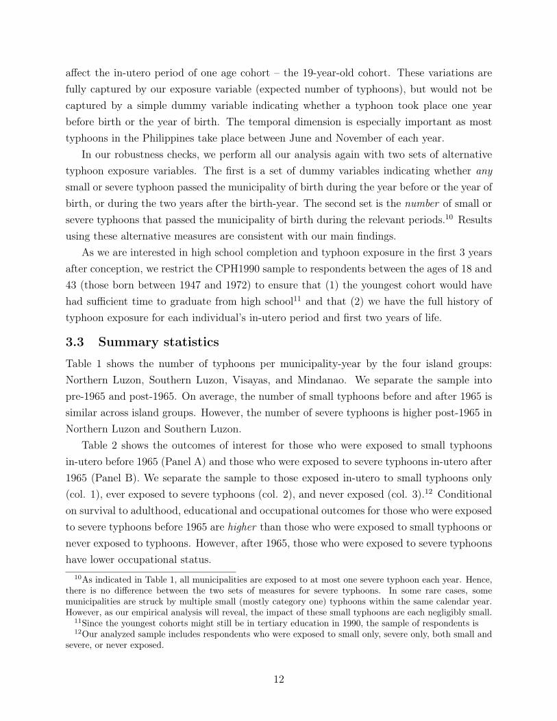
affect the in-utero period of one age cohort – the 19-year-old cohort. These variations arefully captured by our exposure variable (expected number of typhoons), but would not becaptured by a simple dummy variable indicating whether a typhoon took place one yearbefore birth or the year of birth. The temporal dimension is especially important as mosttyphoons in the Philippines take place between June and November of each year.

In our robustness checks, we perform all our analysis again with two sets of alternativetyphoon exposure variables. The first is a set of dummy variables indicating whether anysmall or severe typhoon passed the municipality of birth during the year before or the year ofbirth, or during the two years after the birth-year. The second set is the number of small orsevere typhoons that passed the municipality of birth during the relevant periods.10 Resultsusing these alternative measures are consistent with our main findings.

As we are interested in high school completion and typhoon exposure in the first 3 yearsafter conception, we restrict the CPH1990 sample to respondents between the ages of 18 and43 (those born between 1947 and 1972) to ensure that (1) the youngest cohort would havehad sufficient time to graduate from high school11 and that (2) we have the full history oftyphoon exposure for each individual’s in-utero period and first two years of life.

3.3 Summary statistics

Table 1 shows the number of typhoons per municipality-year by the four island groups:Northern Luzon, Southern Luzon, Visayas, and Mindanao. We separate the sample intopre-1965 and post-1965. On average, the number of small typhoons before and after 1965 issimilar across island groups. However, the number of severe typhoons is higher post-1965 inNorthern Luzon and Southern Luzon.

Table 2 shows the outcomes of interest for those who were exposed to small typhoonsin-utero before 1965 (Panel A) and those who were exposed to severe typhoons in-utero after1965 (Panel B). We separate the sample to those exposed in-utero to small typhoons only(col. 1), ever exposed to severe typhoons (col. 2), and never exposed (col. 3).12 Conditionalon survival to adulthood, educational and occupational outcomes for those who were exposedto severe typhoons before 1965 are higher than those who were exposed to small typhoons ornever exposed to typhoons. However, after 1965, those who were exposed to severe typhoonshave lower occupational status.

10As indicated in Table 1, all municipalities are exposed to at most one severe typhoon each year. Hence,there is no difference between the two sets of measures for severe typhoons. In some rare cases, somemunicipalities are struck by multiple small (mostly category one) typhoons within the same calendar year.However, as our empirical analysis will reveal, the impact of these small typhoons are each negligibly small.

11Since the youngest cohorts might still be in tertiary education in 1990, the sample of respondents is12Our analyzed sample includes respondents who were exposed to small only, severe only, both small and

severe, or never exposed.

12

4 Results

4.1 Estimation strategy

We exploit the temporal and geographical variation of the typhoon paths as well as exogenousvariations in typhoon intensity. We employ a difference-in-differences method exploitingvariations at the cohort-municipality level. Specifically, we compare individuals that areexposed to typhoons either in-utero or in their first two years of life to those that are eitherborn in the same municipality in a different year or born in a different municipality in thesame year and are, therefore, exposed neither in-utero nor in the first two years of theirlives. Subsection 4.2 presents results on mortality, using cohort size and the fraction ofmales in each cohort as outcome variables to infer mortality. Subsection 4.3 presents resultson long-term educational and occupational outcomes.

In subsection 4.4, we extend our analysis to within-household sibling comparisons. Thatis, we compare individuals who were exposed to typhoons either in-utero or in their first twoyears of life to a sibling who was born in a different year and, hence, never exposed duringthe early-life period.

4.2 Cohort size and mortality

We begin by analyzing the effects on mortality. Ideally, there would be detailed data onfetal, infant, child, and adult mortality rates for each cohort born in a given municipality. Inpractice, such mortality records, especially fetal mortality, does not exist for the Philippinesbecause pregnancies are not recorded. We adopt the approach of Jayachandran (2009) andinfer mortality by measuring cohort size based on individuals’ municipality of birth. Theoutcome variable we use is municipality-level cohort size in the 1990 Census. The estimatedeffects will be the cumulative effects of typhoon exposures on fetal, infant, child, and adultmortality. Specifically, we estimate the following equation for each birth-municipality m andbirth-year t,

ln(CohortSize

mt

) = ✓0 small_inutero

mt

+ ✓1 small_postnatal

mt

+ �0 severe_inutero

mt

+ �1 severe_postnatal

mt

+ �

muni

+ ⌧

t

⇥

island

+ �

region

⇥ t+ ✏

mt

(1)

where CohortSize

mt

refers to the number of individuals born in municipality m and yeart that survived until May 1st, 1990. The treatment variable small_inutero measures ex-posure to small typhoons in-utero. Similarly, small_postnatal measures exposure to smalltyphoons in the first and second years of life; severe_inutero and severe_postnatal are the

13

corresponding measures for severe typhoons.In all subsequent analysis, we include municipality fixed effects to take into account

non-time varying municipality characteristics. We also include birth-year by island groupfixed effects, ⌧

t

⇥

island

. We include four island groups in our analysis: North and CentralLuzon, Southern Luzon, Visayas, and Mindanao. These fixed effects allow us to accountfor differences in education and economic development policies across the four island groupsthat may affect the outcome of interest. In addition, we include region-specific time trends,�

region

⇥ t, to allow for differential population growth trends in different regions. We includethirteen different regions.13 Standard errors are clustered two-way at both the municipalityand the province-by-birth-year levels. Clustering by province-year allows us to account forthe spatial correlation across municipalities in typhoon exposure.

One potential caveat of using cohort size to study mortality effects is that cohort sizecan also reflect changes in conception rate. To address this concern, we also present resultsusing the fraction of males in each cohort at the outcome variable. Under the fragile malehypothesis (Kraemer, 2000), adverse early-life shocks would have a larger impact on malemortality rates more than female mortality rates, hence reducing the fraction of males inthe cohort. If, however, the adverse shock reduces the rate of conception rather than fetalor infant mortality rates, we would expect similar reductions in male and female cohort sizeand no change in the fraction of males. Therefore, reductions in the fraction of males wouldprovide suggestive evidence that the changes in cohort size is likely attributable to changesin mortality rather than changes in conception.

Table 4 presents the results of estimating Equation 1. We restrict our sample to cohortsbetween age 2 and 43 in columns 1 to 4. We exclude cohorts aged below 2 or above 43because we do not have the full typhoon exposure information for those cohorts’ (in-utero toage two). In columns 5 to 8, we further restrict our sample to cohorts between age 18 and 43to match the sample we use for education and occupational outcomes. We find that severetyphoons are associated with increased mortality, but not small typhoons. On average, in-utero exposure to one severe typhoon reduces cohort size by about 5 percent, but exposureto a small typhoon has no significant effect on cohort size (column 1). The estimated effectis similar, about 7 percent, when we restrict the sample to ages 18 to 43 (column 5). Ourfinding is consistent with the literature that has documented the adverse effects of exposureto severe early-life negative shocks and suggests a strong dose-response effect to the severityof the shock.

13There are thirteen regions in the Philippines in CPH 1990: National Capital Region, Ilocos Region,Cagayan Valley, Central Luzon, Southern Tagalog, Bicol, Western Visayas, Central Visayas, Eastern Visayas,Western Mindanao, Northern Mindanao, Southern Mindanao, and Central Mindanao.

14

In addition, the mortality effects of exposure to severe typhoons are concentrated amongmales – the effects on male cohort size is large (8 percent) and statistically significant (column2), whereas the effects on female cohort size is much smaller (3 percent) and statisticallyinsignificant (column 3). We also estimate the effects on the fraction of male in each birth-municipality-birth-year (columns 4 and 8). The estimates, albeit imprecise, indicate thatexposure to a severe typhoon reduces the faction of males in each cohort by 1 to 2 percentagepoints, suggesting that the reduction in male cohort size that is driven by increases in early-life mortality rather than reductions in conception. Taken together, these results suggestthat the mortality effects of exposure to severe typhoons are more pronounced among males,which is consistent with the fragile male hypothesis (Kraemer, 2000).

We then examine the changes in mortality after the implementation of disaster reliefpolicies. We separate typhoon exposures according to whether the typhoon occurred beforeor after Marcos assumed office in December 1965 and estimate the following equation:

ln(CohortSize

mt

) = ⇢0 pre_65_small_inutero

mt

+ ⇢1 pre_65_small_postnatal

mt

+ ↵0 pre_65_severe_inutero

mt

+ ↵1 pre_65_severe_postnatal

mt

+ ✓0 post_65_small_inutero

mt

+ ✓1 post_65_small_postnatal

mt

+ �0 post_65_severe_inutero

mt

+ �1 post_65_severe_postnatal

mt

+ �

muni

+ ⌧

t

⇥

island

+ �

region

⇥ t+ ✏

mt

(2)

where the treatment variables small_inutero, small_postnatal, severe_inutero, and severe_postnatal

are interacted with either a pre_65 or a post_65 dummy variable indicating whether thetyphoon exposure took place before or after December 1965. The implicit assumption isthat all typhoons that took place after December 1965 are covered by Ferdinand Marcos’disaster relief policies. We present results using December 1968, the month that the Na-tional Committee on Disaster Operation was established, as the alternative cut-off for pre-and under-Marcos periods in Subsection 4.5.

Table 5 presents the results of estimating Equation 2. The results show stark contrastsof mortality effects before and after 1965. In-utero exposure to a severe pre-1965 typhoonis associated with a statistically significant 10 percent decrease in overall cohort size in 1990(column 1). This effect is also stronger among males (15 percent) compared to females (6percent and not statistically significant). In contrast, the effects of in-utero exposure to asevere post-1965 typhoon is both substantively and statistically insignificant (columns 1-4).The estimates are similar when we restrict the sample size to cohorts between the ages of18 and 43 (columns 5 to 8). Although the effects on the fraction of males are impreciselyestimated, the difference in magnitude is large between pre- and post- 1965 severe typhoons

15

– in-utero exposure to a severe pre-1965 typhoon reduces the fraction of males by 2.23percentage points, whereas in-utero exposure to a severe post-1965 typhoon reduces thefraction of males by 0.583 percentage points. Similar to our earlier findings, the effects ofin-utero exposure to a small typhoon is insignificant in magnitude both before and after1965.

We interpret these as suggestive evidence that the post-disaster relief measures takenby the Marcos government had some effects on reducing the adverse short-term effects oftyphoons. This change in early life mortality can in turn affect the observed long-termscarring effects on the survivors..

4.3 Educational attainment and occupational skill level

Conditional on survival, we estimate the long-term effects of exposure to small and severetyphoons that occurred before and after Marcos took office. We estimate the followingequation:

y

imt

= ⇢0 pre_65_small_inutero

mt

+ ⇢1 pre_65_small_postnatal

mt

+ ↵0 pre_65_severe_inutero

mt

+ ↵1 pre_65_severe_postnatal

mt

+ ✓0 post_65_small_inutero

mt

+ ✓1 post_65_small_postnatal

mt

+ �0 post_65_severe_inutero

mt

+ �1 post_65_severe_postnatal

mt

+ �X

imt

+ �

muni

+ ⌧

t

⇥

island

+ �

region

⇥ t+ ✏

imt

(3)

where y

imt

is the outcome of interest for individual i, born in municipality m, in year t.We include the same set of typhoon exposure variables as in Equation 2, with the implicitassumption that once a municipality is exposed to a typhoon, everyone residing in the mu-nicipality is exposed. Additionally, we include a male indicator as a covariate (X

imt

). Whenusing occupation as the outcome variable, we also include years of education as a covariatein some specifications.

As in Equation 2, we include municipality fixed effects, �muni

, birth-year-by-island-groupfixed effects, ⌧

t

⇥

island

, and region-specific time trends, �region

⇥ t. Standard errors areclustered two-way at both the municipality and the province-by-birth-year level. In addition,observations are weighted by the person weights provided in CPH 1990.

Education Table 6 presents the effects on educational attainment. There is a strong dose-response relationship by the intensity of the typhoon as well as a sharp increase in the scarringeffects after 1965. Exposure to small typhoons, both pre- and post-1965, had little effects

16

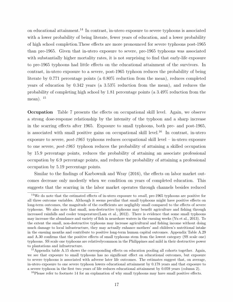
on educational attainment.14 In contrast, in-utero exposure to severe typhoons is associatedwith a lower probability of being literate, fewer years of education, and a lower probabilityof high school completion.These effects are more pronounced for severe typhoons post-1965than pre-1965. Given that in-utero exposure to severe, pre-1965 typhoons was associatedwith substantially higher mortality rates, it is not surprising to find that early-life exposureto pre-1965 typhoons had little effects on the educational attainment of the survivors. Incontrast, in-utero exposure to a severe, post-1965 typhoon reduces the probability of beingliterate by 0.771 percentage points (a 0.80% reduction from the mean), reduces completedyears of education by 0.342 years (a 3.53% reduction from the mean), and reduces theprobability of completing high school by 1.81 percentage points (a 3.49% reduction from themean). 15

Occupation Table 7 presents the effects on occupational skill level. Again, we observea strong dose-response relationship by the intensity of the typhoon and a sharp increasein the scarring effects after 1965. Exposure to small typhoons, both pre- and post-1965,is associated with small positive gains on occupational skill level.16 In contrast, in-uteroexposure to severe, post-1965 typhoons reduces occupational skill level – in-utero exposureto one severe, post-1965 typhoon reduces the probability of attaining a skilled occupationby 15.9 percentage points, reduces the probability of attaining an associate professionaloccupation by 6.9 percentage points, and reduces the probability of attaining a professionaloccupation by 5.19 percentage points.

Similar to the findings of Karbownik and Wray (2016), the effects on labor market out-comes decrease only modestly when we condition on years of completed education. Thissuggests that the scarring in the labor market operates through channels besides reduced

14We do note that the estimated effects of in-utero exposure to small, pre-1965 typhoons are positive forall three outcome variables. Although it seems peculiar that small typhoons might have positive effects onlong-term outcomes, the magnitude of the coefficients are negligibly small compared to the effects of severetyphoons. We also note that small, non-destructive typhoons may benefit agriculture and fishing throughincreased rainfalls and cooler temperature(Lam et al., 2012). There is evidence that some small typhoonsmay increase the abundance and variety of fish in nearshore waters in the ensuing weeks (Yu et al., 2013). Tothe extent the small, non-destructive typhoons may increase agricultural and fishing income without doingmuch damage to local infrastructure, they may actually enhance mothers’ and children’s nutritional intakein the ensuing months and contribute to positive long-term human capital outcomes. Appendix Table A.29and A.30 confirms that the positive effects of small typhoons stem from the lowest category (SS scale one)typhoons. SS scale one typhoons are relativelycommon in the Philippines and mild in their destructive powerto plantations and infrastructure.

15Appendix table A.15 shows the corresponding effects on education pooling all cohorts together. Again,we see that exposure to small typhoons has no significant effect on educational outcomes, but exposureto severe typhoons is associated with adverse later life outcomes. The estimates suggest that, on average,in-utero exposure to one severe typhoon lowers educational attainment by 0.178 years and that exposure toa severe typhoon in the first two years of life reduces educational attainment by 0.059 years (column 2).

16Please refer to footnote 14 for an explanation of why small typhoons may have small positive effects.

17

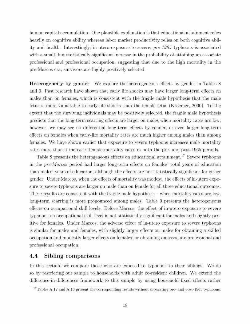
human capital accumulation. One plausible explanation is that educational attainment reliesheavily on cognitive ability whereas labor market productivity relies on both cognitive abil-ity and health. Interestingly, in-utero exposure to severe, pre-1965 typhoons is associatedwith a small, but statistically significant increase in the probability of attaining an associateprofessional and professional occupation, suggesting that due to the high mortality in thepre-Marcos era, survivors are highly positively selected.

Heterogeneity by gender We explore the heterogeneous effects by gender in Tables 8and 9. Past research have shown that early life shocks may have larger long-term effects onmales than on females, which is consistent with the fragile male hypothesis that the malefetus is more vulnerable to early-life shocks than the female fetus (Kraemer, 2000). To theextent that the surviving individuals may be positively selected, the fragile male hypothesispredicts that the long-term scarring effects are larger on males when mortality rates are low;however, we may see no differential long-term effects by gender, or even larger long-termeffects on females when early-life mortality rates are much higher among males than amongfemales. We have shown earlier that exposure to severe typhoons increases male mortalityrates more than it increases female mortality rates in both the pre- and post-1965 periods.

Table 8 presents the heterogeneous effects on educational attainment.17 Severe typhoonsin the pre-Marcos period had larger long-term effects on females’ total years of educationthan males’ years of education, although the effects are not statistically significant for eithergender. Under Marcos, when the effects of mortality was modest, the effects of in-utero expo-sure to severe typhoons are larger on male than on female for all three educational outcomes.These results are consistent with the fragile male hypothesis – when mortality rates are low,long-term scarring is more pronounced among males. Table 9 presents the heterogeneouseffects on occupational skill levels. Before Marcos, the effect of in-utero exposure to severetyphoons on occupational skill level is not statistically significant for males and slightly pos-itive for females. Under Marcos, the adverse effect of in-utero exposure to severe typhoonsis similar for males and females, with slightly larger effects on males for obtaining a skilledoccupation and modestly larger effects on females for obtaining an associate professional andprofessional occupation.

4.4 Sibling comparisons

In this section, we compare those who are exposed to typhoons to their siblings. We doso by restricting our sample to households with adult co-resident children. We extend thedifference-in-differences framework to this sample by using household fixed effects rather

17Tables A.17 and A.16 present the corresponding results without separating pre- and post-1965 typhoons.

18

than municipality fixed effects.Within-household analysis adds to our analysis in three ways. First, this approach con-

trols for any unobserved heterogeneity across households. If the unobserved characteristicsof households residing in typhoon-exposed areas deteriorate over time, perhaps due to mi-gration, then our identifying assumption would be violated and we may over-estimate theeffects of typhoons, especially the post-1965 typhoons. Sibling comparisons address theseconcerns by controlling for heterogeneities across households.

Second, by comparing results with household fixed-effects to results with municipalityfixed-effects, we can provide suggestive evidence of whether post-natal parental investmentscompensate or reinforce the effects of negative pre-natal shocks (Almond et al., 2009). Ifwithin-household sibling comparisons yield smaller effects than cross-household difference-in-differences analyses, parents may have compensated for the negative pre-natal shocks byinvesting more in the affected child after birth (or there may be changes over time in theunobserved heterogeneity of typhoon-exposed households). If, on the other hand, within-household sibling comparisons yield larger effects than the cross-household analyses, it sug-gests that parents reinforce negative pre-natal shocks by investing less in the affected childafter birth.

Third, we further stratify our household sample by parental socioeconomic status toexamine heterogeneities in the effects of typhoons. Low-income households may be morevulnerable to typhoons. In the Philippines, low-income households are more likely to reside inmake-shift houses in squatter areas, along riverbanks, or close to the coast. These houses maybe heavily damaged, if not completely destroyed, by severe typhoons. Wealthy householdsare more likely to live in concrete buildings on high grounds, which may be less damaged oreven remain intact after a severe typhoon. Past research provides evidence that typhoons aremore damaging to low-income families’ household assets than that of high-income families(Huigen and Jens, 2006; Anttila-Hughes and Hsiang, 2013). In addition, wealthy and well-connected families may also have better access to food and clean water after a severe typhoon.There is evidence from recent disasters that politically communities are better able to obtainpost-disaster funds (Atkinson et al., 2014). We, therefore, expect in-utero typhoon exposuresto be more damaging to children born in low-income families.

To conduct within family sibling comparisons, we restrict the sample to households withadult co-resident children – individuals between the age of 18 and 43 who still live in thesame household as his or her parent(s) and whose reported relationship to the householdhead is either “son” or “daughter.” We further restrict the sample to individuals who have atleast one other sibling living in the same household. These sample restrictions allow us toidentify siblings and their parents. However, these restrictions also leave us with a selected

19

sample. We note that respondents in this sample are on average more educated than theoverall population.18

Tables 10 and 11 present the effects on education and occupation, respectively, of theadult co-resident children sample. In both tables, columns (1) to (3) present sibling compar-ison results using household fixed effects, whereas columns (4) to (6) present results usingmunicipality fixed effects on the same sample. The basic patterns found in the cross sec-tion persist when we use household fixed effects. Moreover, comparing columns (1) to (3)to columns (4) to (6) in both tables, the negative effects of in-utero exposure to severetyphoons are larger in magnitude when using household fixed effects than when using mu-nicipality fixed effects – this is true for both pre- and post-1965 typhoons. The differencein the estimated effect under household and municipality fixed effects is more pronouncedfor educational outcomes than for labor market outcomes. These results offer suggestiveevidence that post-natal parental investments may have reinforced the differences betweensiblings caused by negative pre-natal shocks.

Next, we stratify our sample by household socioeconomic status. Ideally, we would use ameasure of family income or wealth around the time of the child’s birth as the yardstick todivide households into low and high-SES sub-samples. In the absence of a direct measure forpast household income or wealth, we use whether the household head has a skilled occupationto divide the sample.19

Tables 12 and 13 present results by household SES. Results suggest that the adverseeffects are substantially lower on high-SES households than on low-SES households – theestimated effects of in-utero exposure to severe typhoons on years of complete education andoccupational skill levels are large in magnitude and statistically significant for the low-SESsample, but smaller and statistically insignificant for the high-SES sample.

What could explain the differential impact by household SES? One possibility is thathigh-SES families have more resources to cope with severe typhoons. They may live in moretyphoon-resistent houses and are more prepared for potential food shortages in the ensuingweeks. Hence, the wealthier the family, the lower a typhoon’s impact on the mother’s psy-chological well-being and nutritional in-take. Another possibility is that parents inhigh-SESfamilies engage in compensating behavior after the child’s birth – enhancing educational andhealth investments on the child who has experienced negative shocks in early life, whereas

18Average education in the main analyzed sample is about 9.4 years, while it is 10.5 years in the adult-coresident household sample.

19We choose this measure because the distribution of household heads’ occupation is quite stable acrossage groups, whereas other variables such as years of completed education vary more by age group. Giventhat household heads in the adult co-resident children sample span across a wide age range and tend to beolder (with an average of 54 years versus 44 years in the CPH), using household head’s occupation allows usto have a time-consistent way of defining household SES.

20

parents in low-SES families with limited resources adopt reinforcing behavior post-birth –reducing investments on the child who has experienced negative shocks in early life. Distin-guishing between these two mechanisms is outside the scope of this paper.

4.5 Robustness

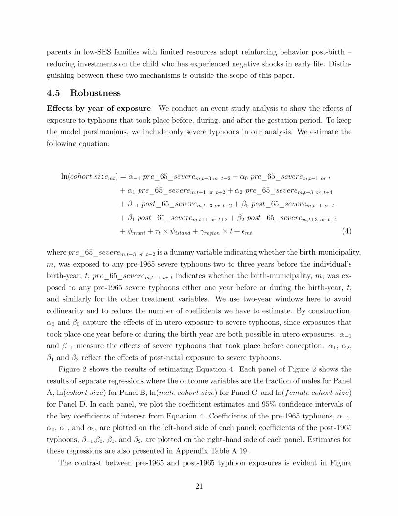
Effects by year of exposure We conduct an event study analysis to show the effects ofexposure to typhoons that took place before, during, and after the gestation period. To keepthe model parsimonious, we include only severe typhoons in our analysis. We estimate thefollowing equation:

ln(cohort sizemt

) = ↵�1 pre_65_severe

m,t�3 or t�2 + ↵0 pre_65_severe

m,t�1 or t

+ ↵1 pre_65_severe

m,t+1 or t+2 + ↵2 pre_65_severe

m,t+3 or t+4

+ ��1 post_65_severe

m,t�3 or t�2 + �0 post_65_severe

m,t�1 or t

+ �1 post_65_severe

m,t+1 or t+2 + �2 post_65_severe

m,t+3 or t+4

+ �

muni

+ ⌧

t

⇥

island

+ �

region

⇥ t+ ✏

mt

(4)

where pre_65_severe

m,t�3 or t�2 is a dummy variable indicating whether the birth-municipality,m, was exposed to any pre-1965 severe typhoons two to three years before the individual’sbirth-year, t; pre_65_severe

m,t�1 or t

indicates whether the birth-municipality, m, was ex-posed to any pre-1965 severe typhoons either one year before or during the birth-year, t;and similarly for the other treatment variables. We use two-year windows here to avoidcollinearity and to reduce the number of coefficients we have to estimate. By construction,↵0 and �0 capture the effects of in-utero exposure to severe typhoons, since exposures thattook place one year before or during the birth-year are both possible in-utero exposures. ↵�1

and ��1 measure the effects of severe typhoons that took place before conception. ↵1, ↵2,�1 and �2 reflect the effects of post-natal exposure to severe typhoons.

Figure 2 shows the results of estimating Equation 4. Each panel of Figure 2 shows theresults of separate regressions where the outcome variables are the fraction of males for PanelA, ln(cohort size) for Panel B, ln(male cohort size) for Panel C, and ln(female cohort size)

for Panel D. In each panel, we plot the coefficient estimates and 95% confidence intervals ofthe key coefficients of interest from Equation 4. Coefficients of the pre-1965 typhoons, ↵�1,↵0, ↵1, and ↵2, are plotted on the left-hand side of each panel; coefficients of the post-1965typhoons, ��1,�0, �1, and �2, are plotted on the right-hand side of each panel. Estimates forthese regressions are also presented in Appendix Table A.19.

The contrast between pre-1965 and post-1965 typhoon exposures is evident in Figure

21

2. The estimates for ↵0 is negative and statistically significant for three outcome variables:fraction of males, cohort size, and male cohort size. In contrast, the estimates for �0 isalmost zero and statistically insignificant for all four outcome variables. These findings areconsistent with our previous results that severe, pre-1965 typhoons substantially reducedcohort size, especially male cohort size, whereas severe, post-1965 typhoons did not.20

Interestingly, however, ↵�1 and ��1 which measure effects of severe typhoons that tookplace before conception (2 to 3 years before birth), are significantly different from zero forsome outcome variables. Our results suggest that pre-conception exposure to severe, pre-1965 typhoons reduces male cohort size by 4 percent, reduces the fraction of males by 0.893percentage points, but has no detectable effects on female cohort size. For severe, post-1965typhoons, our results suggest that pre-conception exposure reduces male cohort size by 2.3percent and reduces female cohort size by 4 percent. The effects on male cohort size (or thefraction of males) is not statistically significant, whereas the effects on female cohort size isstatistically significant.

One channel through which pre-conception typhoon exposures can affect cohort size (andlong-term human outcomes) is reduced household wealth. Anttila-Hughes and Hsiang (2013)find that typhoon exposures reduce household assets and consumption up to three years afterthe initial exposure. It is plausible that those who are severely affected by typhoons needto reduce food consumption even three years after a typhoon in order to save funds forrestoration of their physical assets. Anttila-Hughes and Hsiang (2013) also offer suggestiveevidence that typhoons reduce female infant mortality rates three years after the initialtyphoon exposure. Their study focused on typhoons in the 1980s and the 1990s, whereas ourresults here apply to typhoons between 1945 and 1990. Our results for post-1965 typhoonsare largely consistent with their findings. However, we concede that it is not clear whypre-1965 typhoons affect male cohort size but not female cohort size, whereas post-1965typhoons have the opposite effects.21

20We note that the estimates for ↵0 is - 0.742 when using ln(male cohort size) as the outcome variable.This estimate is much smaller than the corresponding coefficient estimate, -0.144, in Table 5(column 2). Thisis because the treatment variable in Table 5 measures the expected number of in-utero typhoon exposures foreach birth cohort and weights each typhoon that took place one year before or during the birth-year by theprobability that the typhoon took place in-utero for a given birth cohort. The treatment variable here is anindicator of whether any typhoon passed by either one year before or during the year of birth – it may includesome typhoons that took place pre-conception. Nor does it underweight typhoons that took place close tothe end of the birth-year. The estimated effects here are the combined effects of in-utero, pre-conception, andpost-natal exposures. It is, therefore, not surprising that the estimates here are smaller than the estimatesin Table 5. We also used the 1970 Census and find qualitatively similar results on mortality among thoseexposed to severe typhoons pre and post-1965. However, in the 1970 census, we can identify the province ofbirth but not the municipality of birth. The analysis was, thus, done at the province level and the estimatesare not precisely measured. These results are available upon request.

21We also note that, traditionally, most ethnic groups in the Philippines do not practice son preference.

22

Next, we perform the same analysis on long-term human capital outcomes. We estimatethe equivalent of Equation 4 for education and occupational outcomes. We estimate theequation at the individual level and include as control variable a dummy for male. Fig-ure 3 shows the results for fouroutcome variables: years of completed education, having askilled occupation, having an associate professional occupation, and having a professionaloccupation. (Estimates for all educational and occupational outcomes are presented in Ap-pendix Table A.20 and A.21). Again, the contrast between pre-1965 and post-1965 typhoonexposures are made salient. Pre-1965 typhoons had little impact on long-term outcomes.Post-1965 typhoons had large negative effects on both educational attainment and occu-pational skill level; in-utero exposures have the largest impact; post-natal early childhoodexposures have smaller but also substantial impact as well.

Alternative exposure variables In our main analysis, we used the expected numberof typhoons an individual is exposed to as our treatment variable. We assume a linearrelationship between the expected number of exposure and the outcome variables of interest.If some municipalities are exposed to multiple typhoons within a year and if there is a non-linear relationship between the number of exposure and the effects of each exposure, thenEquations 1, 2, 3 would lead to biased estimates. As indicated in Table 1, all municipalitiesare exposed to at most one severe typhoon each year. In less than 1% of municipality-yearpairs, the municipality was struck by multiple small (mostly category one) typhoons withinthe same year. To further alleviate the concerns of a potential non-linear relationship betweenthe number of typhoons exposures and their effects, we compare the results using exposuredummies as treatment variables to the main results using expected number of exposure.This is difficult to do under our setting – for Equations 1, 2, 3, exposure was defined inprobabilities. We expand the analysis in Equation 4 to include small typhoons. We thenreplace the exposure dummies in Equation 4 with count variables indicating the number oftyphoon exposures during each period.

The results show that the non-linearity concerns are minimal. For severe typhoons, thetwo set of treatment variables yield results that are almost identical. This is consistent withthe fact that no municipality was exposed more than one severe typhoon within the sameyear. For small typhoons, although there are some differences between the two set of results,the differences are never statistically significant for any of outcome variables. Moreover, themagnitude of the two sets of estimates are largely consistent with a linear effects model.These results are available upon request.

23

Alternative distance to the eye of the storm One limitation in our study is thatwe do not observe the actual size of the typhoon. In our main analysis, we assume thatmunicipalities and individuals within 30 kilometers of the eye of the storm are affectedby the typhoon and those outside of the 30-kilometer radius are not as affected by thetyphoon. If the size of a typhoon is particularly large such that the wind speed is still ashigh as a category four or five typhoon outside of the 30-kilometer radius, municipalities andindividuals outside of the 30-kilometer radius may be just as affected as those within the30-kilometer radius. If this is the case for some typhoons, our estimates may under-estimatethe adverse effects of typhoons. 22

To test whether the effects of typhoons are beyond the 30-kilometer radius, we add asecond layer of treatment variables assigned to municipalities that are between 30 and 60kilometers away from the eye of the storm. As such, we estimate the effects of typhoonexposure on municipalities and individuals within 30 kilometers of the typhoon path as wellas municipalities and individuals between 30 and 60 kilometers away from the typhoon path.These results are presented in section A.4 of the appendix.

We find that pre-1965 typhoons have little effects on municipalities and individuals 30to 60 kilometers away from the eye of the storm. However, post-1965 typhoons have somenegative effects on the cohort size of municipalities 30 to 60 kilometers away from the eye ofthe storm; these effects are even larger than the effects on municipalities within 30 kilometers.This pattern is unique to cohort size effects – we do not find the same patterns for long-termoutcomes. What could account for the larger adverse effects on municipalities further awayfrom the storm path? One possible explanation is that the size of some post-1965 typhoonsare larger than the size of pre-1965 typhoons, and, more importantly, disaster relief fundingmay be more available for municipalities close to the typhoon path than for municipalitiesfurther away from the typhoon path.

Alternative storm intensity measures Our main analysis allows for only two stormintensity levels (small and severe). We now allow for four different storm intensity categoriesaccording to the Saffir-Simpson (SS) classification system. We continue to combine SS scale4 and scale 5 storms in one category because only a small number of municipalities were everexposed to scale 5 storms.

We find evidence for a strong dose-response effect before the disaster preparedness policy(Table A.28). Category 1 and 2 storms have no significant effect on overall cohort size,

22Brand and Blelloch (1973) documents thatintense typhoons passing the Philippines between 1960 to 1970have an average eye diameter of 20 to 30 miles, which translate to an eye radius of 16 to 24 kilometers. Theyalso found that the intense typhoons have smaller eye diameters but larger circulation sizes than less-intensetyphoons.

24

while category 3 and higher storms are associated with lower cohort size. With the disasterpreparedness policy, we find no significant effect on overall cohort size for the 2-43 year oldsample. Using the restricted sample of 18 to 43 year olds, we find that category 3 stormsare associated with a 7 percent decrease in cohort size. This may be due to the storm being’not severe enough’ for the disaster relief policy to be implemented.

Tables A.29 and A.30 present results on education and occupation respectively. Pre-1965, we find no significant reduction in education among respondents who were exposed totyphoons in early life. We also find no significant reduction in the probability of attaininghigher occupational skill levels among those exposed to typhoons in early life. In fact, insome cases, we see a higher probability of attaining higher occupational status among thoseexposed to typhoons. Post-1965, we find lower literacy among those exposed to category3, 4, and 5 storms in-utero. We also find lower years of education among those exposed inutero to the most severe (categories 4 and 5) storms. We find lower occupational skill levelsamong those exposed to category 2 storms in utero and those exposed to the most severestorms in utero or in their first two years of life. These results are consistent with changingearly life mortality and dose-response effect.

Alternative cutoff year Although Ferdinand Marcos came into office after December1965, drastic changes in disaster relief policy only began in December 1968 after the Casigu-ran earthquake. In our main analysis, we used December 1965 as the cut-off time for policychange. For robustness, we also perform our analysis using December 1968 as the alterna-tive cut-off time for policy change. Appendix Table A.31 presents estimation results usingcohort size as the outcome variable. Appendix Tables A.32 and A.33 present estimationresults using educational attainment and occupational prestige as the outcome variables,respectively.

Whereas the basic patterns found in the main analysis persist, in most cases, using 1968as the cut-off time brings out an even larger contrast between the pre-Marcos and under-Marcos years. Effects on cohort sizes are larger for the pre-Marcos period when we use1968 as the cutoff, whereas cohort size effects for the under-Marcos period become smaller.Effects for most long-term outcomes are still small and insignificant for the pre-Marcosperiod, whereas long-term effects for the post-Marcos period become even larger, especiallyon occupation. These results suggest that the change in the availability of disaster relieffunding after December 1968 is the main contributor to the muted mortality effects in theunder-Marcos period.

25

5 Conclusion

We find a strong dose-response effect to early life exposure to natural disasters in a set-ting where natural disasters occur frequently severe disasters are associated with adverseoutcomes, while less intense events are associated with small or not statistically significanteffects. These findings stand in stark contrast with findings from the U.S. and Brazil whereless severe hurricanes can have large negative effects on both short-term and long-term out-comes (Karbownik and Wray, 2016; Currie and Rossin-Slater, 2013; Simeonova, 2011). Oneplausible explanation for the differences in findings is the role of adaptation. Due to the highfrequency of low intensity typhoons in the Philippines, residents are relatively well adaptedto cope with low intensity typhoons. With adaptation, compared to residents in the U.S. andBrazil, households in the Philippines may be more prepared, both mentally and physically tocope with lower intensity, somewhat expected natural disasters because of the high frequencyof such events in the Philippines. However, our findings suggest that, without the help ofgovernment assistance, residents, and low-SES residents in particular, are not prepared tocope with severe typhoons on their own. Our findings suggest that policy makers shouldtake the severity of natural disaster into account in implementing both short and long terminterventions.

We also find a strong negative relationship between mortality and the long-term scarringeffects. When the mortality effects of severe disasters are especially high (pre-1965 typhoonsin our setting), we do not observe any differences in long-term outcomes between the survivorsand those who were not exposed to the shock at all. When the mortality effects of severedisasters are much more muted (post-1965 typhoons), we observe large differences in long-term outcomes between the survivors and the unaffected. The observed adverse outcomesdue to scarring in low mortality setting reflect improved early life survival. These contrastssuggest that research on early life shocks in developing countries should pay special attentionto selective mortality (Currie and Vogl, 2013).

The provision of post disaster resources in the aftermath of a natural disaster has longbeen the focus in policy making in high income and lower income settings. Our findingssuggest that short term assistance like Ferdinand Marcos’ disaster response policies in thelate 1960s and 1970s have been especially effective in lowering early-life mortality causedby disasters. However, alleviating the scarring effects on long-term outcomes still remains achallenge for future research and for policy making. To that end, our findings that childrenfrom high-SES families in the post-1965 sample were somewhat shielded from the negativeeffects of severe typhoons offer a sense of hope – with strong infrastructure and sufficient post-disaster aid, complete resilience could be within reach even for the most ferocious storms.

26

References

Adhvaryu, A., T. Molina, A. Nyshadham, and J. Tamayo (2015). Helping children catch up:Early life shocks and the progresa experiment.

Almond, D. (2006). Is the 1918 influenza pandemic over? long-term effects of in uteroinfluenza exposure in the post-1940 us population. Journal of political Economy 114 (4),672–712.

Almond, D. and J. Currie (2011). Killing me softly: The fetal origins hypothesis. TheJournal of Economic Perspectives 25 (3), 153–172.

Almond, D., J. Currie, and V. Duque (2017). Childhood circumstances and adult outcomes:Act ii. Technical report, National Bureau of Economic Research.

Almond, D., L. Edlund, and M. Palme (2009). Chernobyl’s subclinical legacy: prenatalexposure to radioactive fallout and school outcomes in sweden. The Quarterly journal ofeconomics 124 (4), 1729–1772.

Almond, D. and B. Mazumder (2013). Fetal origins and parental responses. Annu. Rev.Econ. 5 (1), 37–56.

Almond, D., B. Mazumder, and R. Ewijk (2015). In utero ramadan exposure and children’sacademic performance. The Economic Journal 125 (589), 1501–1533.

Almond, D. and B. A. Mazumder (2011). Health capital and the prenatal environment: theeffect of ramadan observance during pregnancy. American Economic Journal: AppliedEconomics 3 (4), 56–85.

Anttila-Hughes, J. K. and S. M. Hsiang (2013). Destruction, disinvestment, and death:Economic and human losses following environmental disaster. Available at SSRN 2220501 .

Arceo, E., R. Hanna, and P. Oliva (2016). Does the effect of pollution on infant mortal-ity differ between developing and developed countries? evidence from mexico city. TheEconomic Journal .

Atkinson, J., A. Hicken, and N. Ravanilla (2014). Pork and typhoons: The influence ofpolitical connections on disaster response.

Barker, D. J. (1995). Fetal origins of coronary heart disease. BMJ: British Medical Jour-nal 311 (6998), 171.

27

Brand, S. and J. W. Blelloch (1973). Changes in the characteristics of typhoons crossing thephilippines. Journal of Applied Meteorology 12 (1), 104–109.

Carballo, M., M. Hernandez, K. Schneider, and E. Welle (2005). Impact of the tsunami onreproductive health. Journal of the Royal Society of Medicine 98 (9), 400–403.

Celoza, A. F. (1997). Ferdinand Marcos and the Philippines: the political economy of au-thoritarianism. Greenwood Publishing Group.

Cunha, F. and J. Heckman (2007). The economics of human development: The technologyof skill formation. The American economic review 97 (2), 31–47.

Currie, J. and D. Almond (2011). Human capital development before age five. Handbook oflabor economics 4, 1315–1486.

Currie, J. and M. Rossin-Slater (2013). Weathering the storm: Hurricanes and birth out-comes. Journal of health economics 32 (3), 487–503.

Currie, J. and T. Vogl (2013). Early-life health and adult circumstance in developing coun-tries. Annu. Rev. Econ 5, 1–36.

Deaton, A. (2007). Height, health, and development. Proceedings of the National Academyof Sciences 104 (33), 13232–13237.

Deuchert, E. and C. Felfe (2015). The tempest: Short-and long-term consequences of anatural disaster for children’s development. European Economic Review 80, 280–294.

Doocy, S., A. Rofi, C. Moodie, E. Spring, S. Bradley, G. Burnham, and C. Robinson (2007).Tsunami mortality in aceh province, indonesia. Bulletin of the World Health Organiza-tion 85 (4), 273–278.

Frankenberg, E., J. Friedman, N. Ingwerson, and D. Thomas (2013). Child height after anatural disaster. Duke University .

Frankenberg, E., T. Gillespie, S. Preston, B. Sikoki, and D. Thomas (2011). Mortality, thefamily and the indian ocean tsunami. The Economic Journal 121 (554), F162–F182.

Franklin, S. and J. Labonne (2016). Economic shocks and labour market flexibility.

Gunnsteinsson, S., A. Adhvaryu, P. Christian, A. Labrique, J. Sugimoto, A. A. Shamim,and K. P. West Jr (2016). Resilience to early life shocks: Evidence from the interactionof a natural experiment and a randomized control trial.

28

Hanna, R. and P. Oliva (2016). Implications of climate change for children in developingcountries. The Future of Children, 115–132.

Hsiang, S. M. and A. S. Jina (2014). The causal effect of environmental catastrophe onlong-run economic growth: Evidence from 6,700 cyclones.

Huigen, M. G. and I. C. Jens (2006). Socio-economic impact of super typhoon harurot insan mariano, isabela, the philippines. World Development 34 (12), 2116–2136.

Jayachandran, S. (2009). Air quality and early-life mortality evidence from indonesia’swildfires. Journal of Human Resources 44 (4), 916–954.

Kannisto, V., K. Christensen, and J. W. Vaupel (1997). No increased mortality in later lifefor cohorts bom during famine. American Journal of Epidemiology 145 (11), 987–994.

Karbownik, K. and A. Wray (2016). Long-run consequences of exposure to natural disasters.

Knapp, K. R., J. A. Knaff, C. R. Sampson, G. M. Riggio, and A. D. Schnapp (2013). Apressure-based analysis of the historical western north pacific tropical cyclone intensityrecord. Monthly Weather Review 141 (8), 2611–2631.

Kraemer, S. (2000). The fragile male. British Medical Journal 321 (7276), 1609.

Lam, H., M. H. Kok, and K. K. Y. Shum (2012). Benefits from typhoons–the hong kongperspective. Weather 67 (1), 16–21.

Lin, M.-J. and E. M. Liu (2014). Does in utero exposure to illness matter? the 1918 influenzaepidemic in taiwan as a natural experiment. Journal of health economics 37, 152–163.

Liu, E., J.-T. Liu, and T.-Y. H. Tseng (2016). Fetal origins of mental health: Evidence fromnatural disasters in taiwan.

Meng, X. and N. Qian (2009). The long term consequences of famine on survivors: evidencefrom a unique natural experiment using china’s great famine. Technical report, NationalBureau of Economic Research.

Rosales, M. F. and M. Triyana (2016). The persistent effects of early-life exposure to airpollution: Evidence from the indonesian forest fires.

Simeonova, E. (2011). Out of sight, out of mind? natural disasters and pregnancy outcomesin the usa. Cesifo Economic Studies 57 (3), 403–431(29).

29

Ugaz, J. and A. Zanolini (2011). Effects of extreme weather shocks during pregnancy andearly life on later health outcomes: the case of philippines typhoons.

Warren, J. F. (2013). A tale of two decades: Typhoons and floods, manila and the provinces,and the marcos years. The Asia-Pacific Journal 11, 43.

Yu, J., D. Tang, Y. Li, Z. Huang, and G. Chen (2013). Increase in fish abundance duringtwo typhoons in the south china sea. Advances in Space Research 51 (9), 1734–1749.

Zivin, J. S. G., S. M. Hsiang, and M. J. Neidell (2015). Temperature and human capital inthe short-and long-run.

30

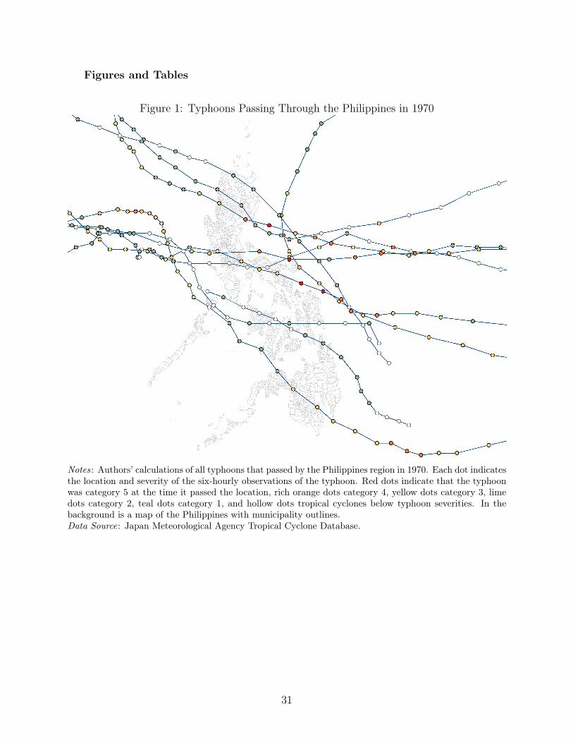
Figures and Tables

Figure 1: Typhoons Passing Through the Philippines in 1970

Notes: Authors’ calculations of all typhoons that passed by the Philippines region in 1970. Each dot indicatesthe location and severity of the six-hourly observations of the typhoon. Red dots indicate that the typhoonwas category 5 at the time it passed the location, rich orange dots category 4, yellow dots category 3, limedots category 2, teal dots category 1, and hollow dots tropical cyclones below typhoon severities. In thebackground is a map of the Philippines with municipality outlines.Data Source: Japan Meteorological Agency Tropical Cyclone Database.

31

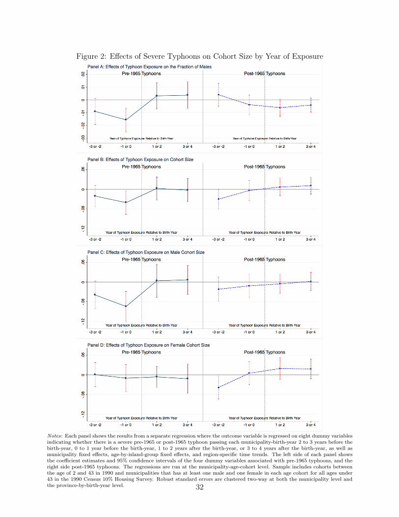
Figure 2: Effects of Severe Typhoons on Cohort Size by Year of Exposure

Notes: Each panel shows the results from a separate regression where the outcome variable is regressed on eight dummy variablesindicating whether there is a severe pre-1965 or post-1965 typhoon passing each municipality-birth-year 2 to 3 years before thebirth-year, 0 to 1 year before the birth-year, 1 to 2 years after the birth-year, or 3 to 4 years after the birth-year, as well asmunicipality fixed effects, age-by-island-group fixed effects, and region-specific time trends. The left side of each panel showsthe coefficient estimates and 95% confidence intervals of the four dummy variables associated with pre-1965 typhoons, and theright side post-1965 typhoons. The regressions are run at the municipality-age-cohort level. Sample includes cohorts betweenthe age of 2 and 43 in 1990 and municipalities that has at least one male and one female in each age cohort for all ages under43 in the 1990 Census 10% Housing Survey. Robust standard errors are clustered two-way at both the municipality level andthe province-by-birth-year level. 32

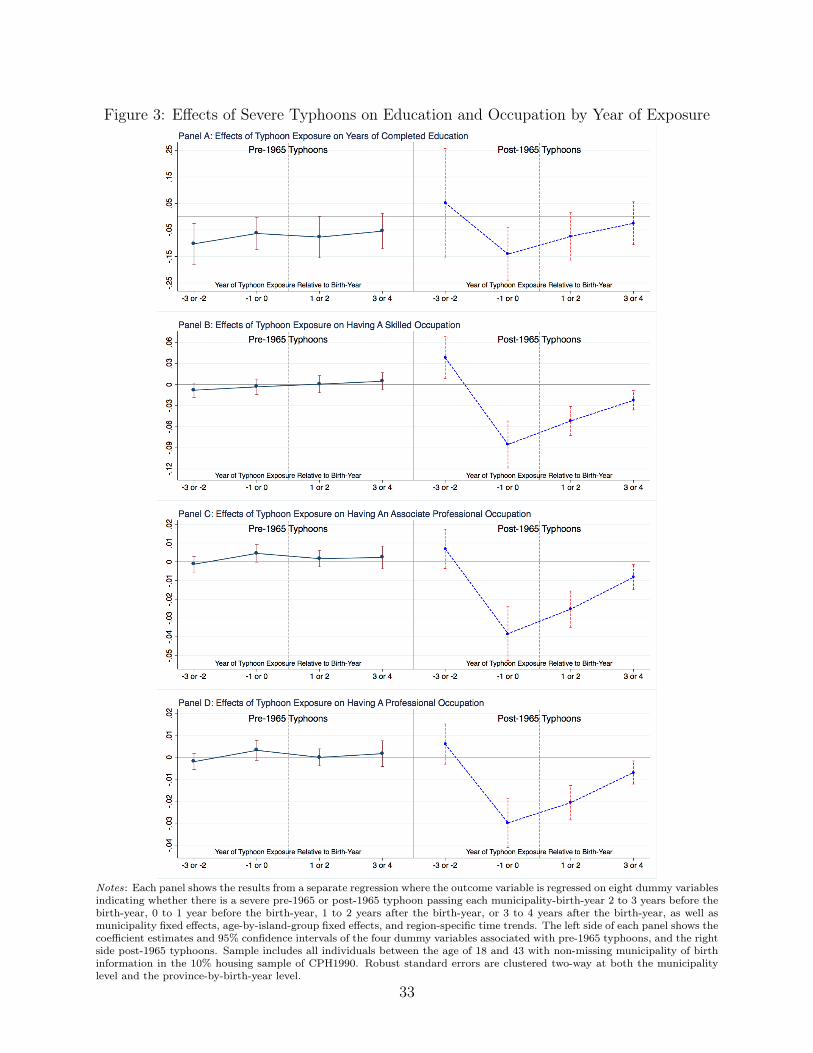
Figure 3: Effects of Severe Typhoons on Education and Occupation by Year of Exposure

Notes: Each panel shows the results from a separate regression where the outcome variable is regressed on eight dummy variablesindicating whether there is a severe pre-1965 or post-1965 typhoon passing each municipality-birth-year 2 to 3 years before thebirth-year, 0 to 1 year before the birth-year, 1 to 2 years after the birth-year, or 3 to 4 years after the birth-year, as well asmunicipality fixed effects, age-by-island-group fixed effects, and region-specific time trends. The left side of each panel shows thecoefficient estimates and 95% confidence intervals of the four dummy variables associated with pre-1965 typhoons, and the rightside post-1965 typhoons. Sample includes all individuals between the age of 18 and 43 with non-missing municipality of birthinformation in the 10% housing sample of CPH1990. Robust standard errors are clustered two-way at both the municipalitylevel and the province-by-birth-year level.

33

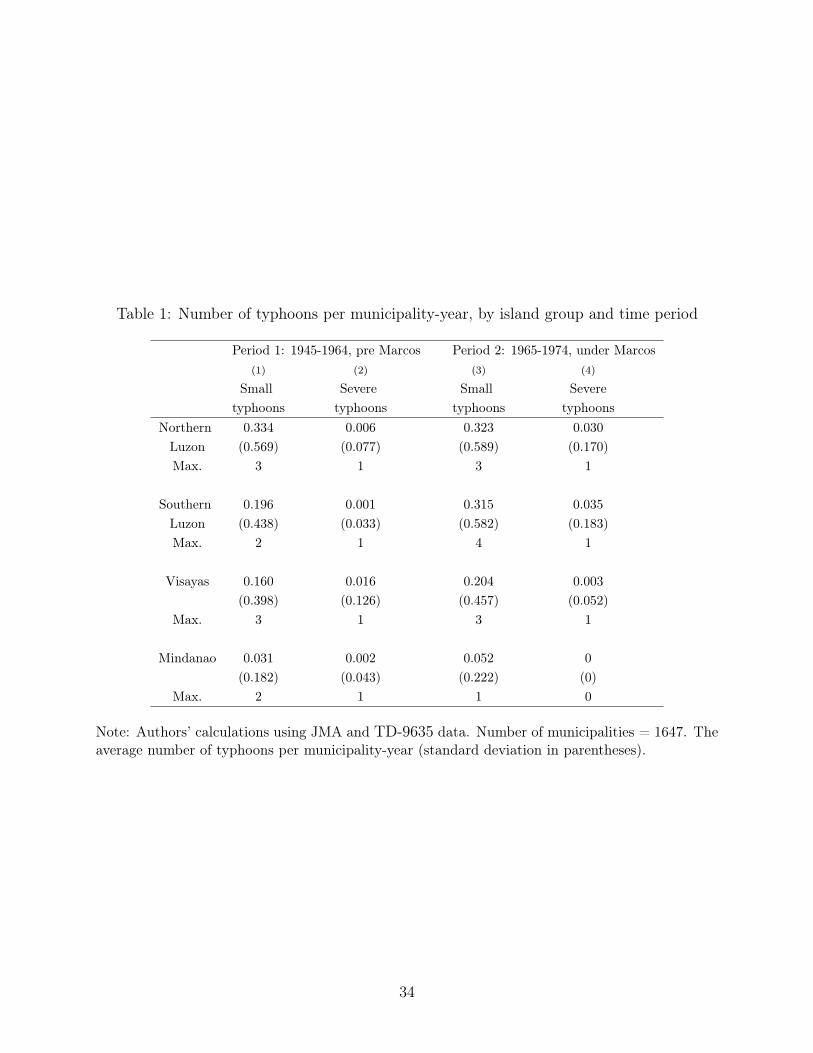
Table 1: Number of typhoons per municipality-year, by island group and time period

Period 1: 1945-1964, pre Marcos Period 2: 1965-1974, under Marcos(1) (2) (3) (4)

Small Severe Small Severetyphoons typhoons typhoons typhoons

Northern 0.334 0.006 0.323 0.030Luzon (0.569) (0.077) (0.589) (0.170)Max. 3 1 3 1

Southern 0.196 0.001 0.315 0.035Luzon (0.438) (0.033) (0.582) (0.183)Max. 2 1 4 1

Visayas 0.160 0.016 0.204 0.003(0.398) (0.126) (0.457) (0.052)

Max. 3 1 3 1

Mindanao 0.031 0.002 0.052 0(0.182) (0.043) (0.222) (0)

Max. 2 1 1 0

Note: Authors’ calculations using JMA and TD-9635 data. Number of municipalities = 1647. Theaverage number of typhoons per municipality-year (standard deviation in parentheses).

34

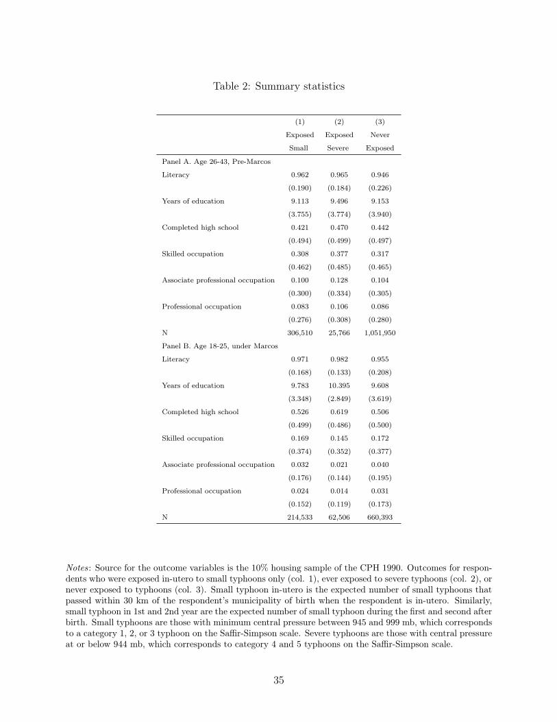
Table 2: Summary statistics

(1) (2) (3)

Exposed Exposed Never

Small Severe Exposed

Panel A. Age 26-43, Pre-Marcos

Literacy 0.962 0.965 0.946

(0.190) (0.184) (0.226)

Years of education 9.113 9.496 9.153

(3.755) (3.774) (3.940)

Completed high school 0.421 0.470 0.442

(0.494) (0.499) (0.497)

Skilled occupation 0.308 0.377 0.317

(0.462) (0.485) (0.465)

Associate professional occupation 0.100 0.128 0.104

(0.300) (0.334) (0.305)

Professional occupation 0.083 0.106 0.086

(0.276) (0.308) (0.280)

N 306,510 25,766 1,051,950

Panel B. Age 18-25, under Marcos

Literacy 0.971 0.982 0.955

(0.168) (0.133) (0.208)

Years of education 9.783 10.395 9.608

(3.348) (2.849) (3.619)

Completed high school 0.526 0.619 0.506

(0.499) (0.486) (0.500)

Skilled occupation 0.169 0.145 0.172

(0.374) (0.352) (0.377)

Associate professional occupation 0.032 0.021 0.040

(0.176) (0.144) (0.195)

Professional occupation 0.024 0.014 0.031

(0.152) (0.119) (0.173)

N 214,533 62,506 660,393

Notes: Source for the outcome variables is the 10% housing sample of the CPH 1990. Outcomes for respon-dents who were exposed in-utero to small typhoons only (col. 1), ever exposed to severe typhoons (col. 2), ornever exposed to typhoons (col. 3). Small typhoon in-utero is the expected number of small typhoons thatpassed within 30 km of the respondent’s municipality of birth when the respondent is in-utero. Similarly,small typhoon in 1st and 2nd year are the expected number of small typhoon during the first and second afterbirth. Small typhoons are those with minimum central pressure between 945 and 999 mb, which correspondsto a category 1, 2, or 3 typhoon on the Saffir-Simpson scale. Severe typhoons are those with central pressureat or below 944 mb, which corresponds to category 4 and 5 typhoons on the Saffir-Simpson scale.

35

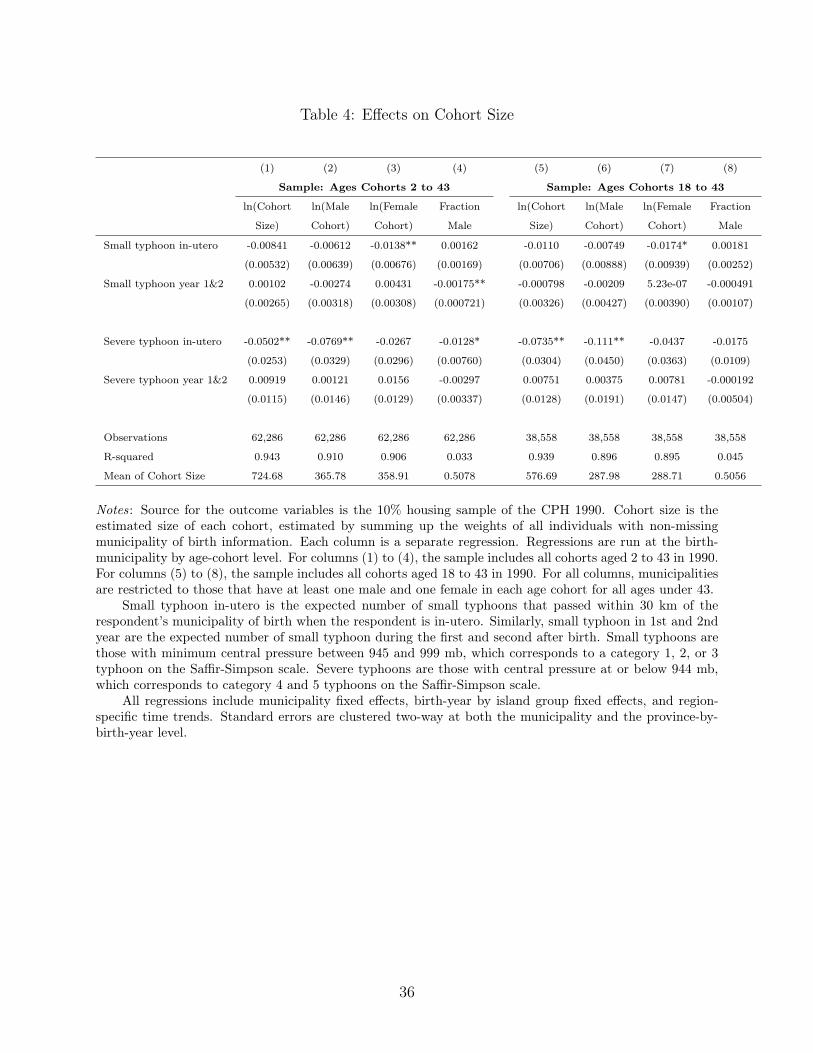
Table 4: Effects on Cohort Size

(1) (2) (3) (4) (5) (6) (7) (8)

Sample: Ages Cohorts 2 to 43 Sample: Ages Cohorts 18 to 43

ln(Cohort ln(Male ln(Female Fraction ln(Cohort ln(Male ln(Female Fraction

Size) Cohort) Cohort) Male Size) Cohort) Cohort) Male

Small typhoon in-utero -0.00841 -0.00612 -0.0138** 0.00162 -0.0110 -0.00749 -0.0174* 0.00181

(0.00532) (0.00639) (0.00676) (0.00169) (0.00706) (0.00888) (0.00939) (0.00252)

Small typhoon year 1&2 0.00102 -0.00274 0.00431 -0.00175** -0.000798 -0.00209 5.23e-07 -0.000491

(0.00265) (0.00318) (0.00308) (0.000721) (0.00326) (0.00427) (0.00390) (0.00107)

Severe typhoon in-utero -0.0502** -0.0769** -0.0267 -0.0128* -0.0735** -0.111** -0.0437 -0.0175

(0.0253) (0.0329) (0.0296) (0.00760) (0.0304) (0.0450) (0.0363) (0.0109)

Severe typhoon year 1&2 0.00919 0.00121 0.0156 -0.00297 0.00751 0.00375 0.00781 -0.000192

(0.0115) (0.0146) (0.0129) (0.00337) (0.0128) (0.0191) (0.0147) (0.00504)

Observations 62,286 62,286 62,286 62,286 38,558 38,558 38,558 38,558

R-squared 0.943 0.910 0.906 0.033 0.939 0.896 0.895 0.045

Mean of Cohort Size 724.68 365.78 358.91 0.5078 576.69 287.98 288.71 0.5056

Notes: Source for the outcome variables is the 10% housing sample of the CPH 1990. Cohort size is theestimated size of each cohort, estimated by summing up the weights of all individuals with non-missingmunicipality of birth information. Each column is a separate regression. Regressions are run at the birth-municipality by age-cohort level. For columns (1) to (4), the sample includes all cohorts aged 2 to 43 in 1990.For columns (5) to (8), the sample includes all cohorts aged 18 to 43 in 1990. For all columns, municipalitiesare restricted to those that have at least one male and one female in each age cohort for all ages under 43.

Small typhoon in-utero is the expected number of small typhoons that passed within 30 km of therespondent’s municipality of birth when the respondent is in-utero. Similarly, small typhoon in 1st and 2ndyear are the expected number of small typhoon during the first and second after birth. Small typhoons arethose with minimum central pressure between 945 and 999 mb, which corresponds to a category 1, 2, or 3typhoon on the Saffir-Simpson scale. Severe typhoons are those with central pressure at or below 944 mb,which corresponds to category 4 and 5 typhoons on the Saffir-Simpson scale.

All regressions include municipality fixed effects, birth-year by island group fixed effects, and region-specific time trends. Standard errors are clustered two-way at both the municipality and the province-by-birth-year level.

36

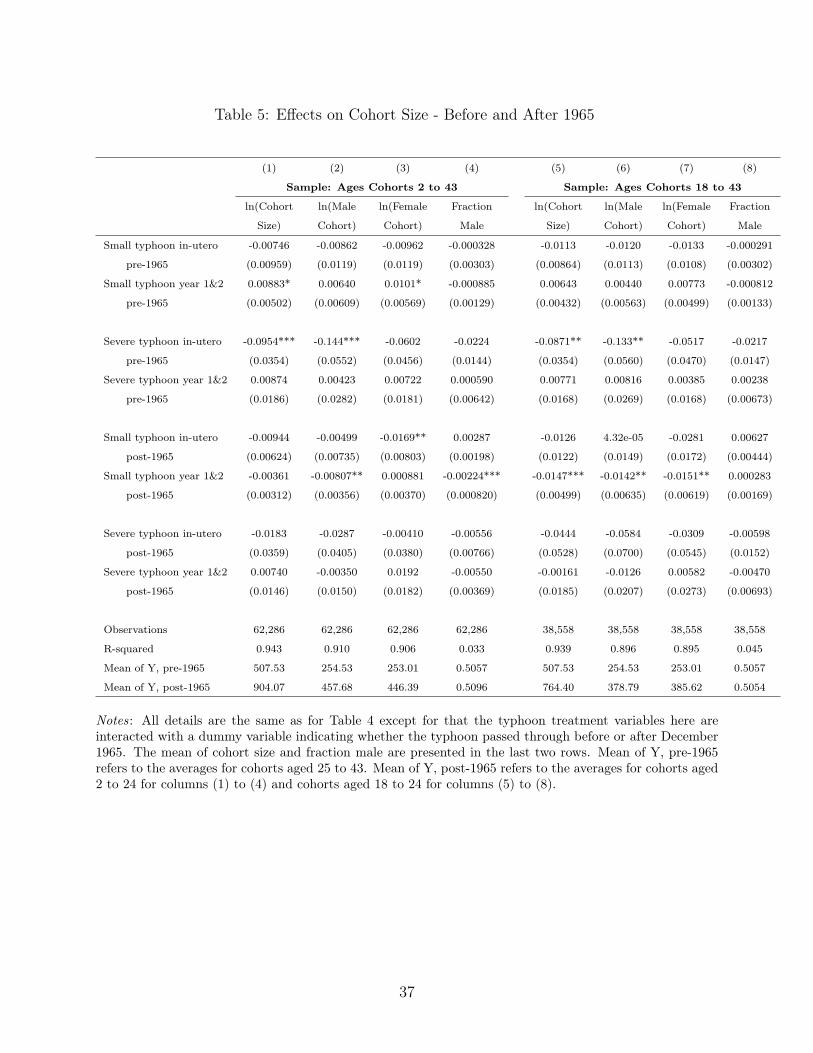
Table 5: Effects on Cohort Size - Before and After 1965

(1) (2) (3) (4) (5) (6) (7) (8)

Sample: Ages Cohorts 2 to 43 Sample: Ages Cohorts 18 to 43

ln(Cohort ln(Male ln(Female Fraction ln(Cohort ln(Male ln(Female Fraction

Size) Cohort) Cohort) Male Size) Cohort) Cohort) Male

Small typhoon in-utero -0.00746 -0.00862 -0.00962 -0.000328 -0.0113 -0.0120 -0.0133 -0.000291

pre-1965 (0.00959) (0.0119) (0.0119) (0.00303) (0.00864) (0.0113) (0.0108) (0.00302)

Small typhoon year 1&2 0.00883* 0.00640 0.0101* -0.000885 0.00643 0.00440 0.00773 -0.000812

pre-1965 (0.00502) (0.00609) (0.00569) (0.00129) (0.00432) (0.00563) (0.00499) (0.00133)

Severe typhoon in-utero -0.0954*** -0.144*** -0.0602 -0.0224 -0.0871** -0.133** -0.0517 -0.0217

pre-1965 (0.0354) (0.0552) (0.0456) (0.0144) (0.0354) (0.0560) (0.0470) (0.0147)

Severe typhoon year 1&2 0.00874 0.00423 0.00722 0.000590 0.00771 0.00816 0.00385 0.00238

pre-1965 (0.0186) (0.0282) (0.0181) (0.00642) (0.0168) (0.0269) (0.0168) (0.00673)

Small typhoon in-utero -0.00944 -0.00499 -0.0169** 0.00287 -0.0126 4.32e-05 -0.0281 0.00627

post-1965 (0.00624) (0.00735) (0.00803) (0.00198) (0.0122) (0.0149) (0.0172) (0.00444)

Small typhoon year 1&2 -0.00361 -0.00807** 0.000881 -0.00224*** -0.0147*** -0.0142** -0.0151** 0.000283

post-1965 (0.00312) (0.00356) (0.00370) (0.000820) (0.00499) (0.00635) (0.00619) (0.00169)

Severe typhoon in-utero -0.0183 -0.0287 -0.00410 -0.00556 -0.0444 -0.0584 -0.0309 -0.00598

post-1965 (0.0359) (0.0405) (0.0380) (0.00766) (0.0528) (0.0700) (0.0545) (0.0152)

Severe typhoon year 1&2 0.00740 -0.00350 0.0192 -0.00550 -0.00161 -0.0126 0.00582 -0.00470

post-1965 (0.0146) (0.0150) (0.0182) (0.00369) (0.0185) (0.0207) (0.0273) (0.00693)

Observations 62,286 62,286 62,286 62,286 38,558 38,558 38,558 38,558

R-squared 0.943 0.910 0.906 0.033 0.939 0.896 0.895 0.045

Mean of Y, pre-1965 507.53 254.53 253.01 0.5057 507.53 254.53 253.01 0.5057

Mean of Y, post-1965 904.07 457.68 446.39 0.5096 764.40 378.79 385.62 0.5054

Notes: All details are the same as for Table 4 except for that the typhoon treatment variables here areinteracted with a dummy variable indicating whether the typhoon passed through before or after December1965. The mean of cohort size and fraction male are presented in the last two rows. Mean of Y, pre-1965refers to the averages for cohorts aged 25 to 43. Mean of Y, post-1965 refers to the averages for cohorts aged2 to 24 for columns (1) to (4) and cohorts aged 18 to 24 for columns (5) to (8).

37

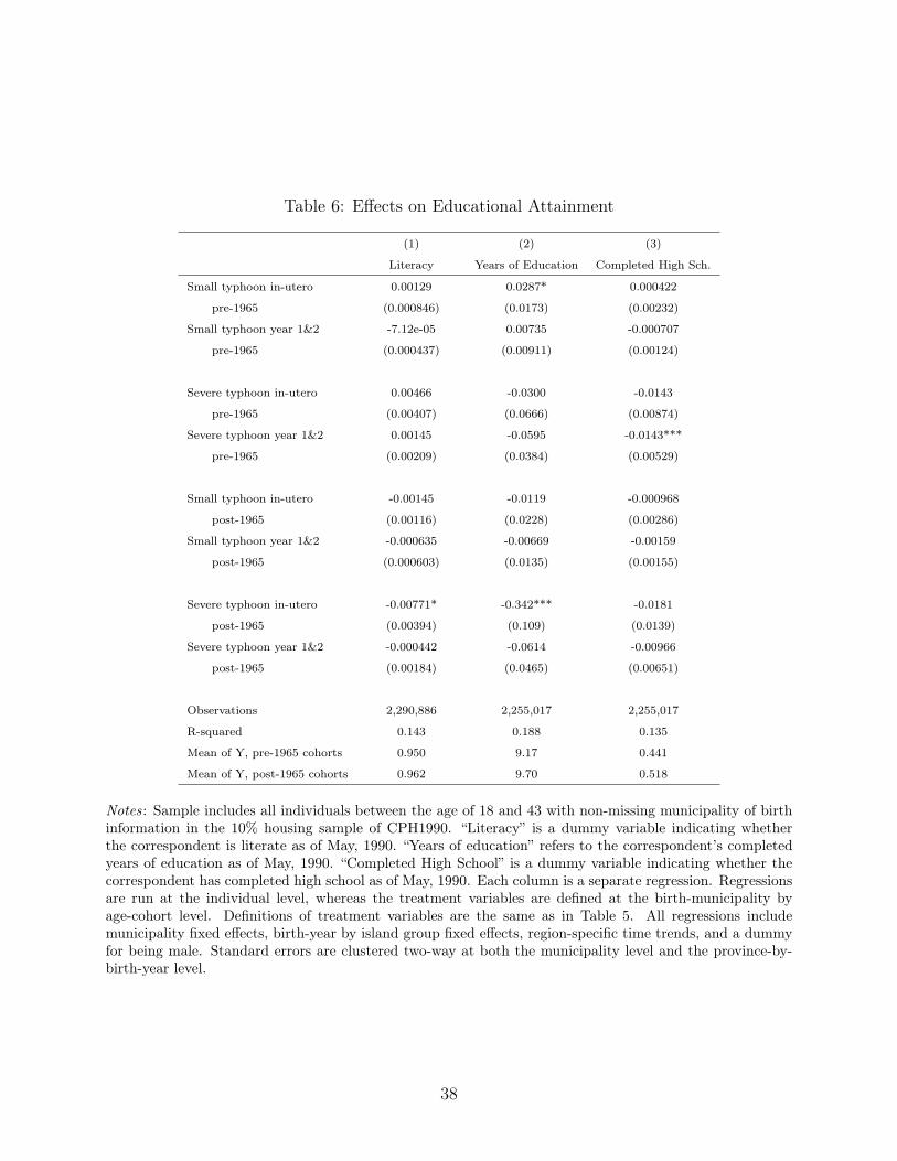
Table 6: Effects on Educational Attainment

(1) (2) (3)

Literacy Years of Education Completed High Sch.

Small typhoon in-utero 0.00129 0.0287* 0.000422

pre-1965 (0.000846) (0.0173) (0.00232)

Small typhoon year 1&2 -7.12e-05 0.00735 -0.000707

pre-1965 (0.000437) (0.00911) (0.00124)

Severe typhoon in-utero 0.00466 -0.0300 -0.0143

pre-1965 (0.00407) (0.0666) (0.00874)

Severe typhoon year 1&2 0.00145 -0.0595 -0.0143***

pre-1965 (0.00209) (0.0384) (0.00529)

Small typhoon in-utero -0.00145 -0.0119 -0.000968

post-1965 (0.00116) (0.0228) (0.00286)

Small typhoon year 1&2 -0.000635 -0.00669 -0.00159

post-1965 (0.000603) (0.0135) (0.00155)

Severe typhoon in-utero -0.00771* -0.342*** -0.0181

post-1965 (0.00394) (0.109) (0.0139)

Severe typhoon year 1&2 -0.000442 -0.0614 -0.00966

post-1965 (0.00184) (0.0465) (0.00651)

Observations 2,290,886 2,255,017 2,255,017

R-squared 0.143 0.188 0.135

Mean of Y, pre-1965 cohorts 0.950 9.17 0.441

Mean of Y, post-1965 cohorts 0.962 9.70 0.518

Notes: Sample includes all individuals between the age of 18 and 43 with non-missing municipality of birthinformation in the 10% housing sample of CPH1990. “Literacy” is a dummy variable indicating whetherthe correspondent is literate as of May, 1990. “Years of education” refers to the correspondent’s completedyears of education as of May, 1990. “Completed High School” is a dummy variable indicating whether thecorrespondent has completed high school as of May, 1990. Each column is a separate regression. Regressionsare run at the individual level, whereas the treatment variables are defined at the birth-municipality byage-cohort level. Definitions of treatment variables are the same as in Table 5. All regressions includemunicipality fixed effects, birth-year by island group fixed effects, region-specific time trends, and a dummyfor being male. Standard errors are clustered two-way at both the municipality level and the province-by-birth-year level.

38

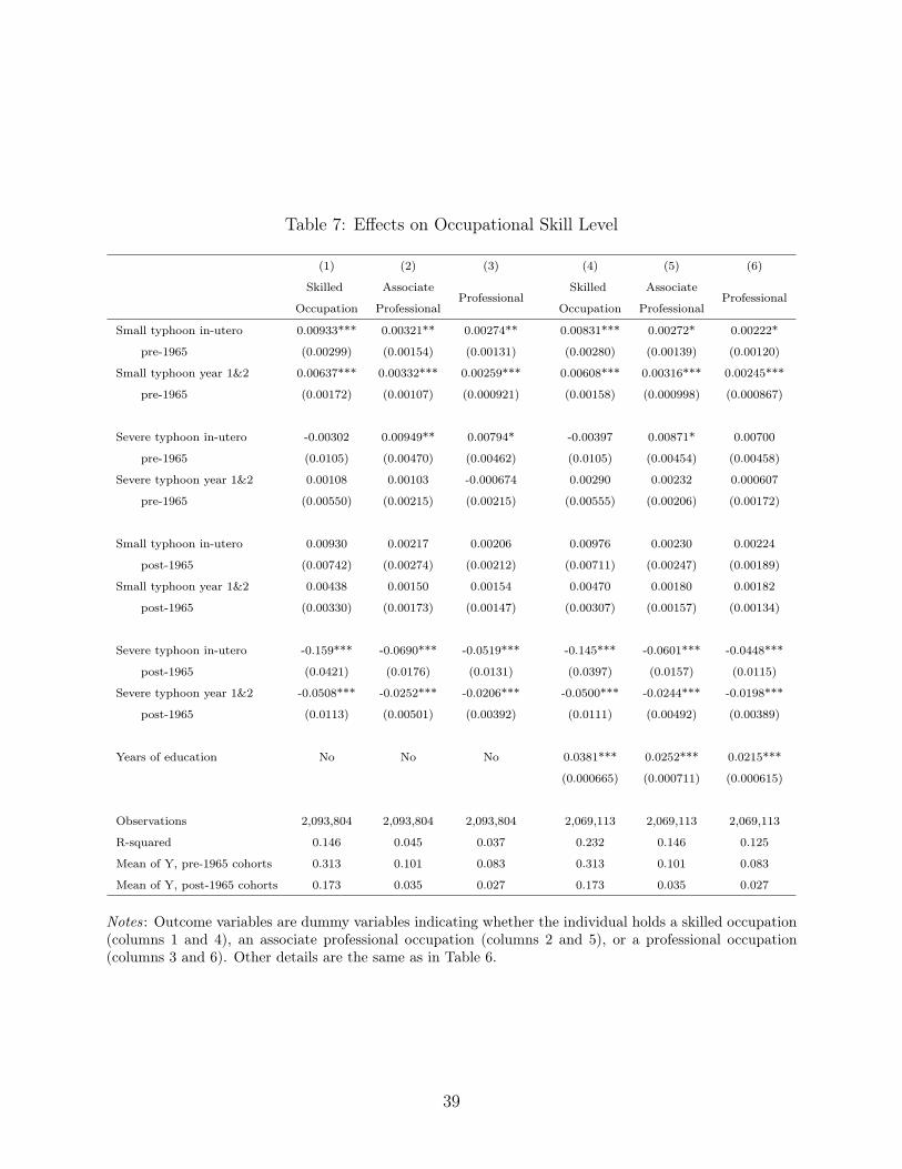
Table 7: Effects on Occupational Skill Level

(1) (2) (3) (4) (5) (6)

Skilled AssociateProfessional

Skilled AssociateProfessional

Occupation Professional Occupation Professional

Small typhoon in-utero 0.00933*** 0.00321** 0.00274** 0.00831*** 0.00272* 0.00222*

pre-1965 (0.00299) (0.00154) (0.00131) (0.00280) (0.00139) (0.00120)

Small typhoon year 1&2 0.00637*** 0.00332*** 0.00259*** 0.00608*** 0.00316*** 0.00245***

pre-1965 (0.00172) (0.00107) (0.000921) (0.00158) (0.000998) (0.000867)

Severe typhoon in-utero -0.00302 0.00949** 0.00794* -0.00397 0.00871* 0.00700

pre-1965 (0.0105) (0.00470) (0.00462) (0.0105) (0.00454) (0.00458)

Severe typhoon year 1&2 0.00108 0.00103 -0.000674 0.00290 0.00232 0.000607

pre-1965 (0.00550) (0.00215) (0.00215) (0.00555) (0.00206) (0.00172)

Small typhoon in-utero 0.00930 0.00217 0.00206 0.00976 0.00230 0.00224

post-1965 (0.00742) (0.00274) (0.00212) (0.00711) (0.00247) (0.00189)

Small typhoon year 1&2 0.00438 0.00150 0.00154 0.00470 0.00180 0.00182

post-1965 (0.00330) (0.00173) (0.00147) (0.00307) (0.00157) (0.00134)

Severe typhoon in-utero -0.159*** -0.0690*** -0.0519*** -0.145*** -0.0601*** -0.0448***

post-1965 (0.0421) (0.0176) (0.0131) (0.0397) (0.0157) (0.0115)

Severe typhoon year 1&2 -0.0508*** -0.0252*** -0.0206*** -0.0500*** -0.0244*** -0.0198***

post-1965 (0.0113) (0.00501) (0.00392) (0.0111) (0.00492) (0.00389)

Years of education No No No 0.0381*** 0.0252*** 0.0215***

(0.000665) (0.000711) (0.000615)

Observations 2,093,804 2,093,804 2,093,804 2,069,113 2,069,113 2,069,113

R-squared 0.146 0.045 0.037 0.232 0.146 0.125

Mean of Y, pre-1965 cohorts 0.313 0.101 0.083 0.313 0.101 0.083

Mean of Y, post-1965 cohorts 0.173 0.035 0.027 0.173 0.035 0.027

Notes: Outcome variables are dummy variables indicating whether the individual holds a skilled occupation(columns 1 and 4), an associate professional occupation (columns 2 and 5), or a professional occupation(columns 3 and 6). Other details are the same as in Table 6.

39

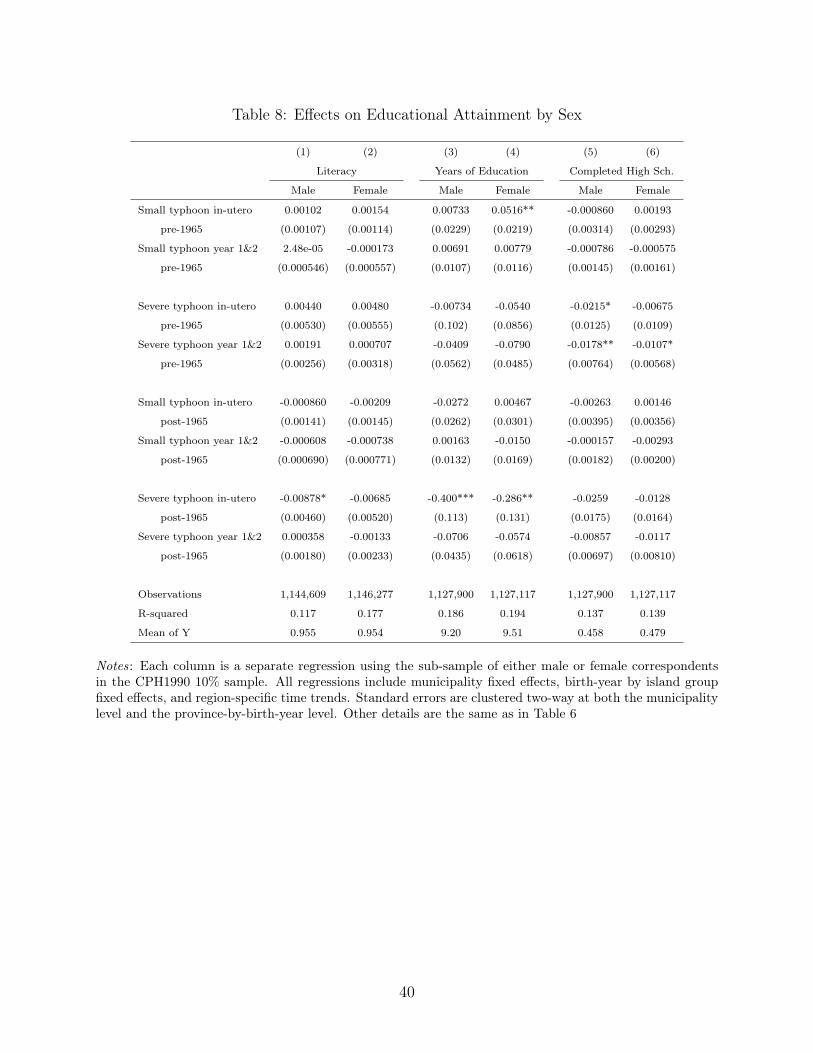
Table 8: Effects on Educational Attainment by Sex

(1) (2) (3) (4) (5) (6)

Literacy Years of Education Completed High Sch.

Male Female Male Female Male Female

Small typhoon in-utero 0.00102 0.00154 0.00733 0.0516** -0.000860 0.00193

pre-1965 (0.00107) (0.00114) (0.0229) (0.0219) (0.00314) (0.00293)

Small typhoon year 1&2 2.48e-05 -0.000173 0.00691 0.00779 -0.000786 -0.000575

pre-1965 (0.000546) (0.000557) (0.0107) (0.0116) (0.00145) (0.00161)

Severe typhoon in-utero 0.00440 0.00480 -0.00734 -0.0540 -0.0215* -0.00675

pre-1965 (0.00530) (0.00555) (0.102) (0.0856) (0.0125) (0.0109)

Severe typhoon year 1&2 0.00191 0.000707 -0.0409 -0.0790 -0.0178** -0.0107*

pre-1965 (0.00256) (0.00318) (0.0562) (0.0485) (0.00764) (0.00568)

Small typhoon in-utero -0.000860 -0.00209 -0.0272 0.00467 -0.00263 0.00146

post-1965 (0.00141) (0.00145) (0.0262) (0.0301) (0.00395) (0.00356)

Small typhoon year 1&2 -0.000608 -0.000738 0.00163 -0.0150 -0.000157 -0.00293

post-1965 (0.000690) (0.000771) (0.0132) (0.0169) (0.00182) (0.00200)

Severe typhoon in-utero -0.00878* -0.00685 -0.400*** -0.286** -0.0259 -0.0128

post-1965 (0.00460) (0.00520) (0.113) (0.131) (0.0175) (0.0164)

Severe typhoon year 1&2 0.000358 -0.00133 -0.0706 -0.0574 -0.00857 -0.0117

post-1965 (0.00180) (0.00233) (0.0435) (0.0618) (0.00697) (0.00810)

Observations 1,144,609 1,146,277 1,127,900 1,127,117 1,127,900 1,127,117

R-squared 0.117 0.177 0.186 0.194 0.137 0.139

Mean of Y 0.955 0.954 9.20 9.51 0.458 0.479

Notes: Each column is a separate regression using the sub-sample of either male or female correspondentsin the CPH1990 10% sample. All regressions include municipality fixed effects, birth-year by island groupfixed effects, and region-specific time trends. Standard errors are clustered two-way at both the municipalitylevel and the province-by-birth-year level. Other details are the same as in Table 6

40

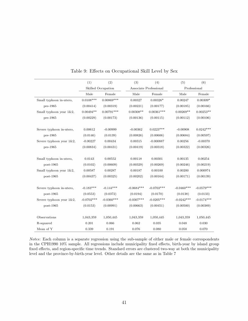
Table 9: Effects on Occupational Skill Level by Sex

(1) (2) (3) (4) (5) (6)

Skilled Occupation Associate Professional Professional

Male Female Male Female Male Female

Small typhoon in-utero, 0.0108*** 0.00869*** 0.00327 0.00326* 0.00247 0.00309*

pre-1965 (0.00414) (0.00319) (0.00221) (0.00177) (0.00185) (0.00166)

Small typhoon year 1&2, 0.00494** 0.00791*** 0.00308** 0.00361*** 0.00269** 0.00253**

pre-1965 (0.00229) (0.00173) (0.00136) (0.00115) (0.00112) (0.00106)

Severe typhoon in-utero, 0.00612 -0.00999 -0.00362 0.0223*** -0.00908 0.0242***

pre-1965 (0.0146) (0.0139) (0.00826) (0.00606) (0.00684) (0.00597)

Severe typhoon year 1&2, -0.00227 0.00434 0.00315 -0.000887 0.00256 -0.00370

pre-1965 (0.00834) (0.00431) (0.00419) (0.00318) (0.00322) (0.00326)

Small typhoon in-utero, 0.0143 0.00552 0.00118 0.00301 0.00135 0.00254

post-1965 (0.0102) (0.00609) (0.00329) (0.00269) (0.00246) (0.00219)

Small typhoon year 1&2, 0.00587 0.00287 0.00187 0.00100 0.00200 0.000974

post-1965 (0.00437) (0.00325) (0.00202) (0.00164) (0.00171) (0.00139)

Severe typhoon in-utero, -0.183*** -0.144*** -0.0684*** -0.0703*** -0.0460*** -0.0579***

post-1965 (0.0553) (0.0372) (0.0194) (0.0170) (0.0138) (0.0133)

Severe typhoon year 1&2, -0.0702*** -0.0360*** -0.0307*** -0.0205*** -0.0242*** -0.0174***

post-1965 (0.0153) (0.00991) (0.00663) (0.00451) (0.00500) (0.00389)

Observations 1,043,359 1,050,445 1,043,359 1,050,445 1,043,359 1,050,445

R-squared 0.201 0.066 0.062 0.035 0.048 0.030

Mean of Y 0.339 0.191 0.076 0.080 0.058 0.070

Notes: Each column is a separate regression using the sub-sample of either male or female correspondentsin the CPH1990 10% sample. All regressions include municipality fixed effects, birth-year by island groupfixed effects, and region-specific time trends. Standard errors are clustered two-way at both the municipalitylevel and the province-by-birth-year level. Other details are the same as in Table 7

41

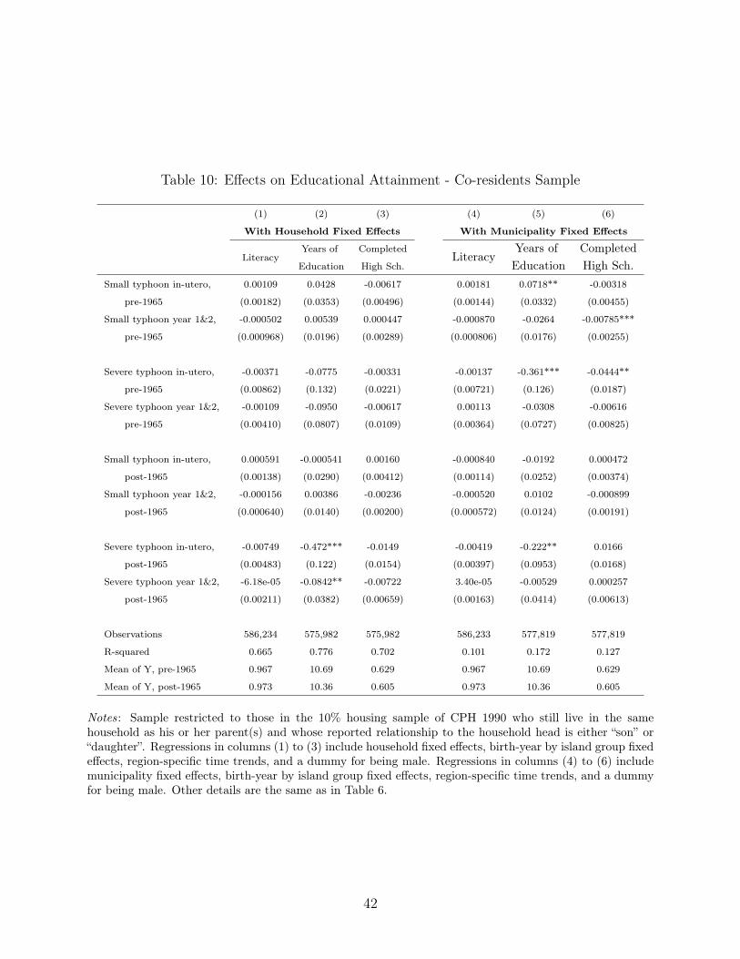
Table 10: Effects on Educational Attainment - Co-residents Sample

(1) (2) (3) (4) (5) (6)

With Household Fixed Effects With Municipality Fixed Effects

LiteracyYears of Completed

LiteracyYears of Completed

Education High Sch. Education High Sch.Small typhoon in-utero, 0.00109 0.0428 -0.00617 0.00181 0.0718** -0.00318

pre-1965 (0.00182) (0.0353) (0.00496) (0.00144) (0.0332) (0.00455)

Small typhoon year 1&2, -0.000502 0.00539 0.000447 -0.000870 -0.0264 -0.00785***

pre-1965 (0.000968) (0.0196) (0.00289) (0.000806) (0.0176) (0.00255)

Severe typhoon in-utero, -0.00371 -0.0775 -0.00331 -0.00137 -0.361*** -0.0444**

pre-1965 (0.00862) (0.132) (0.0221) (0.00721) (0.126) (0.0187)

Severe typhoon year 1&2, -0.00109 -0.0950 -0.00617 0.00113 -0.0308 -0.00616

pre-1965 (0.00410) (0.0807) (0.0109) (0.00364) (0.0727) (0.00825)

Small typhoon in-utero, 0.000591 -0.000541 0.00160 -0.000840 -0.0192 0.000472

post-1965 (0.00138) (0.0290) (0.00412) (0.00114) (0.0252) (0.00374)

Small typhoon year 1&2, -0.000156 0.00386 -0.00236 -0.000520 0.0102 -0.000899

post-1965 (0.000640) (0.0140) (0.00200) (0.000572) (0.0124) (0.00191)

Severe typhoon in-utero, -0.00749 -0.472*** -0.0149 -0.00419 -0.222** 0.0166

post-1965 (0.00483) (0.122) (0.0154) (0.00397) (0.0953) (0.0168)

Severe typhoon year 1&2, -6.18e-05 -0.0842** -0.00722 3.40e-05 -0.00529 0.000257

post-1965 (0.00211) (0.0382) (0.00659) (0.00163) (0.0414) (0.00613)

Observations 586,234 575,982 575,982 586,233 577,819 577,819

R-squared 0.665 0.776 0.702 0.101 0.172 0.127

Mean of Y, pre-1965 0.967 10.69 0.629 0.967 10.69 0.629

Mean of Y, post-1965 0.973 10.36 0.605 0.973 10.36 0.605

Notes: Sample restricted to those in the 10% housing sample of CPH 1990 who still live in the samehousehold as his or her parent(s) and whose reported relationship to the household head is either “son” or“daughter”. Regressions in columns (1) to (3) include household fixed effects, birth-year by island group fixedeffects, region-specific time trends, and a dummy for being male. Regressions in columns (4) to (6) includemunicipality fixed effects, birth-year by island group fixed effects, region-specific time trends, and a dummyfor being male. Other details are the same as in Table 6.

42

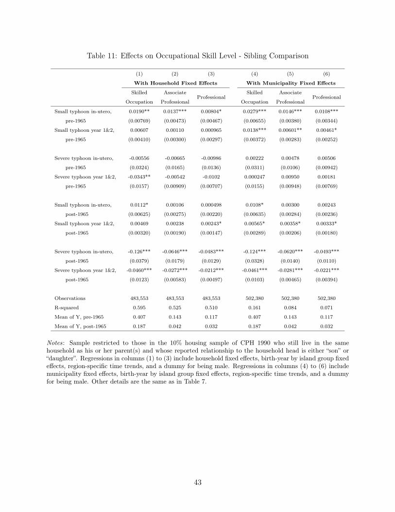
Table 11: Effects on Occupational Skill Level - Sibling Comparison

(1) (2) (3) (4) (5) (6)

With Household Fixed Effects With Municipality Fixed Effects

Skilled AssociateProfessional

Skilled AssociateProfessional

Occupation Professional Occupation Professional

Small typhoon in-utero, 0.0190** 0.0137*** 0.00804* 0.0279*** 0.0146*** 0.0108***

pre-1965 (0.00769) (0.00473) (0.00467) (0.00655) (0.00380) (0.00344)

Small typhoon year 1&2, 0.00607 0.00110 0.000965 0.0138*** 0.00601** 0.00461*

pre-1965 (0.00410) (0.00300) (0.00297) (0.00372) (0.00283) (0.00252)

Severe typhoon in-utero, -0.00556 -0.00665 -0.00986 0.00222 0.00478 0.00506

pre-1965 (0.0324) (0.0165) (0.0136) (0.0311) (0.0106) (0.00942)

Severe typhoon year 1&2, -0.0343** -0.00542 -0.0102 0.000247 0.00950 0.00181

pre-1965 (0.0157) (0.00909) (0.00707) (0.0155) (0.00948) (0.00769)

Small typhoon in-utero, 0.0112* 0.00106 0.000498 0.0108* 0.00300 0.00243

post-1965 (0.00625) (0.00275) (0.00220) (0.00635) (0.00284) (0.00236)

Small typhoon year 1&2, 0.00469 0.00238 0.00243* 0.00565* 0.00358* 0.00333*

post-1965 (0.00320) (0.00190) (0.00147) (0.00289) (0.00206) (0.00180)

Severe typhoon in-utero, -0.126*** -0.0646*** -0.0483*** -0.124*** -0.0620*** -0.0493***

post-1965 (0.0379) (0.0179) (0.0129) (0.0328) (0.0140) (0.0110)

Severe typhoon year 1&2, -0.0460*** -0.0272*** -0.0212*** -0.0461*** -0.0281*** -0.0221***

post-1965 (0.0123) (0.00583) (0.00497) (0.0103) (0.00465) (0.00394)

Observations 483,553 483,553 483,553 502,380 502,380 502,380

R-squared 0.595 0.525 0.510 0.161 0.084 0.071

Mean of Y, pre-1965 0.407 0.143 0.117 0.407 0.143 0.117

Mean of Y, post-1965 0.187 0.042 0.032 0.187 0.042 0.032

Notes: Sample restricted to those in the 10% housing sample of CPH 1990 who still live in the samehousehold as his or her parent(s) and whose reported relationship to the household head is either “son” or“daughter”. Regressions in columns (1) to (3) include household fixed effects, birth-year by island group fixedeffects, region-specific time trends, and a dummy for being male. Regressions in columns (4) to (6) includemunicipality fixed effects, birth-year by island group fixed effects, region-specific time trends, and a dummyfor being male. Other details are the same as in Table 7.

43

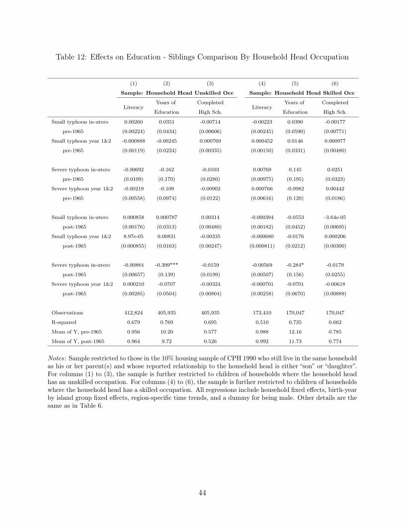
Table 12: Effects on Education - Siblings Comparison By Household Head Occupation

(1) (2) (3) (4) (5) (6)

Sample: Household Head Unskilled Occ Sample: Household Head Skilled Occ

LiteracyYears of Completed

LiteracyYears of Completed

Education High Sch. Education High Sch.

Small typhoon in-utero 0.00260 0.0351 -0.00714 -0.00223 0.0390 -0.00177

pre-1965 (0.00224) (0.0434) (0.00606) (0.00245) (0.0590) (0.00771)

Small typhoon year 1&2 -0.000888 -0.00245 0.000769 0.000452 0.0146 0.000977

pre-1965 (0.00119) (0.0224) (0.00335) (0.00150) (0.0331) (0.00480)

Severe typhoon in-utero -0.00692 -0.162 -0.0103 0.00769 0.145 0.0251

pre-1965 (0.0109) (0.170) (0.0280) (0.00975) (0.195) (0.0323)

Severe typhoon year 1&2 -0.00219 -0.109 -0.00902 0.000766 -0.0982 0.00442

pre-1965 (0.00558) (0.0974) (0.0122) (0.00616) (0.120) (0.0186)

Small typhoon in-utero 0.000858 0.000787 0.00314 -0.000394 -0.0553 -3.64e-05

post-1965 (0.00176) (0.0313) (0.00480) (0.00182) (0.0452) (0.00695)

Small typhoon year 1&2 8.97e-05 0.00831 -0.00335 -0.000680 -0.0176 0.000206

post-1965 (0.000855) (0.0163) (0.00247) (0.000811) (0.0212) (0.00300)

Severe typhoon in-utero -0.00884 -0.399*** -0.0159 -0.00569 -0.284* -0.0179

post-1965 (0.00657) (0.139) (0.0199) (0.00507) (0.156) (0.0255)

Severe typhoon year 1&2 0.000210 -0.0707 -0.00324 -0.000701 -0.0701 -0.00618

post-1965 (0.00285) (0.0504) (0.00804) (0.00258) (0.0670) (0.00889)

Observations 412,824 405,935 405,935 173,410 170,047 170,047

R-squared 0.679 0.769 0.695 0.510 0.735 0.662

Mean of Y, pre-1965 0.956 10.20 0.577 0.988 12.16 0.785

Mean of Y, post-1965 0.964 9.72 0.526 0.992 11.73 0.774

Notes: Sample restricted to those in the 10% housing sample of CPH 1990 who still live in the same householdas his or her parent(s) and whose reported relationship to the household head is either “son” or “daughter”.For columns (1) to (3), the sample is further restricted to children of households where the household headhas an unskilled occupation. For columns (4) to (6), the sample is further restricted to children of householdswhere the household head has a skilled occupation. All regressions include household fixed effects, birth-yearby island group fixed effects, region-specific time trends, and a dummy for being male. Other details are thesame as in Table 6.

44

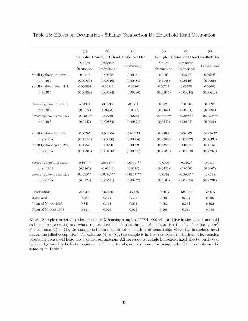
Table 13: Effects on Occupation - Siblings Comparison By Household Head Occupation

(1) (2) (3) (4) (5) (6)

Sample: Household Head Unskilled Occ Sample: Household Head Skilled Occ

Skilled AssociateProfessional

Skilled AssociateProfessional

Occupation Professional Occupation Professional

Small typhoon in-utero, 0.0110 0.00478 0.00151 0.0190 0.0275** 0.0184*

pre-1965 (0.00856) (0.00526) (0.00484) (0.0148) (0.0119) (0.0109)

Small typhoon year 1&2, 0.000901 -0.00341 -0.00262 0.00717 0.00735 0.00609

pre-1965 (0.00399) (0.00284) (0.00296) (0.00855) (0.00644) (0.00613)

Severe typhoon in-utero, -0.0341 -0.0298 -0.0216 0.0623 0.0566 0.0195

pre-1965 (0.0277) (0.0203) (0.0177) (0.0454) (0.0394) (0.0295)

Severe typhoon year 1&2, -0.0300** 0.00232 0.00233 -0.0774*** -0.0466** -0.0630***

pre-1965 (0.0147) (0.00884) (0.00824) (0.0240) (0.0194) (0.0180)

Small typhoon in-utero, 0.00705 -0.000598 -0.000151 0.00993 0.000870 -0.000827

post-1965 (0.00554) (0.00256) (0.00206) (0.00909) (0.00522) (0.00436)

Small typhoon year 1&2, 0.00333 0.00220 0.00199 0.00235 0.000274 0.00154

post-1965 (0.00300) (0.00156) (0.00127) (0.00486) (0.00318) (0.00269)

Severe typhoon in-utero, -0.107*** -0.0531*** -0.0391*** -0.0569 -0.0402* -0.0316*

post-1965 (0.0362) (0.0161) (0.0119) (0.0386) (0.0226) (0.0167)

Severe typhoon year 1&2, -0.0340*** -0.0176*** -0.0149*** -0.0218 -0.0204** -0.0118

post-1965 (0.0120) (0.00531) (0.00457) (0.0168) (0.00864) (0.00731)

Observations 345,476 345,476 345,476 138,077 138,077 138,077

R-squared 0.587 0.512 0.496 0.599 0.539 0.526

Mean of Y, pre-1965 0.345 0.114 0.094 0.602 0.234 0.192

Mean of Y, post-1965 0.151 0.029 0.023 0.266 0.071 0.054

Notes: Sample restricted to those in the 10% housing sample of CPH 1990 who still live in the same householdas his or her parent(s) and whose reported relationship to the household head is either “son” or “daughter”.For columns (1) to (3), the sample is further restricted to children of households where the household headhas an unskilled occupation. For columns (4) to (6), the sample is further restricted to children of householdswhere the household head has a skilled occupation. All regressions include household fixed effects, birth-yearby island group fixed effects, region-specific time trends, and a dummy for being male. Other details are thesame as in Table 7.

45

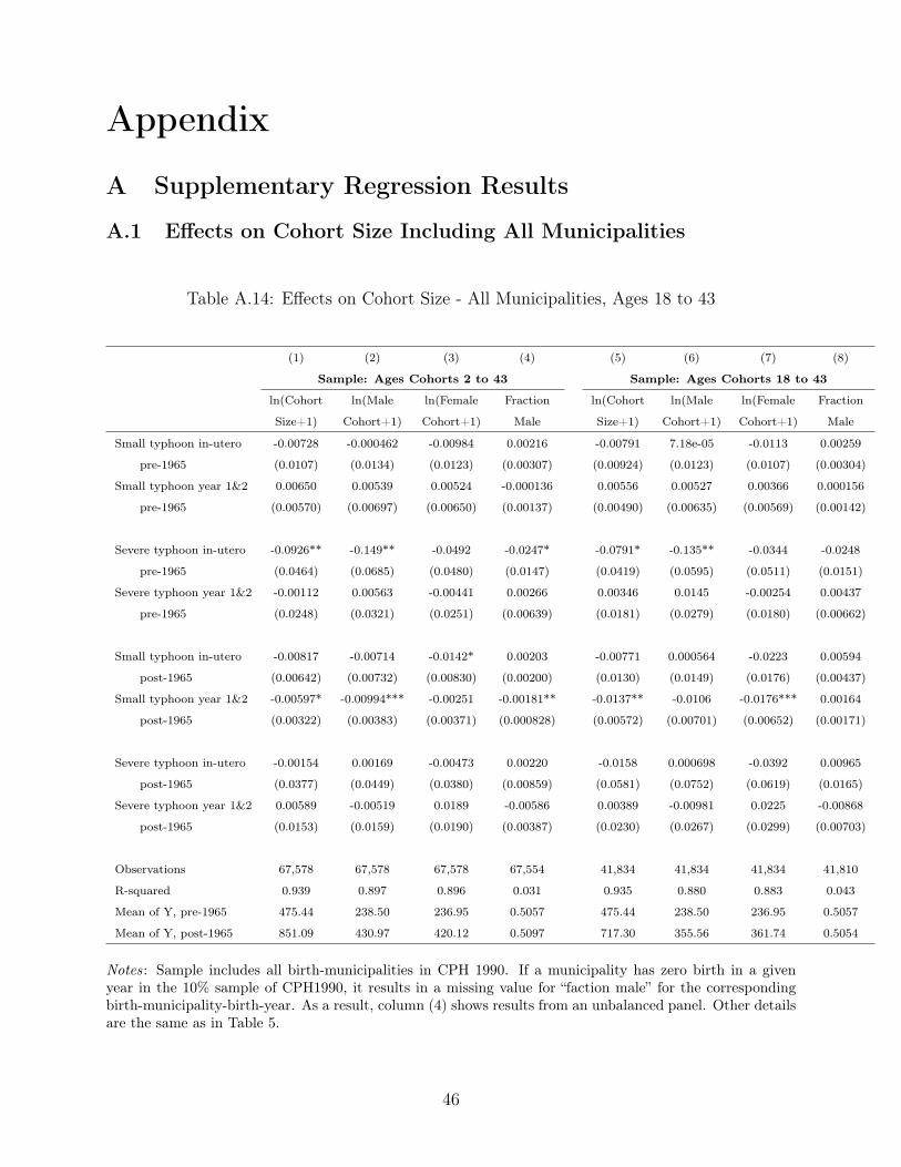
Appendix

A Supplementary Regression Results

A.1 Effects on Cohort Size Including All Municipalities

Table A.14: Effects on Cohort Size - All Municipalities, Ages 18 to 43

(1) (2) (3) (4) (5) (6) (7) (8)

Sample: Ages Cohorts 2 to 43 Sample: Ages Cohorts 18 to 43

ln(Cohort ln(Male ln(Female Fraction ln(Cohort ln(Male ln(Female Fraction

Size+1) Cohort+1) Cohort+1) Male Size+1) Cohort+1) Cohort+1) Male

Small typhoon in-utero -0.00728 -0.000462 -0.00984 0.00216 -0.00791 7.18e-05 -0.0113 0.00259

pre-1965 (0.0107) (0.0134) (0.0123) (0.00307) (0.00924) (0.0123) (0.0107) (0.00304)

Small typhoon year 1&2 0.00650 0.00539 0.00524 -0.000136 0.00556 0.00527 0.00366 0.000156

pre-1965 (0.00570) (0.00697) (0.00650) (0.00137) (0.00490) (0.00635) (0.00569) (0.00142)

Severe typhoon in-utero -0.0926** -0.149** -0.0492 -0.0247* -0.0791* -0.135** -0.0344 -0.0248

pre-1965 (0.0464) (0.0685) (0.0480) (0.0147) (0.0419) (0.0595) (0.0511) (0.0151)

Severe typhoon year 1&2 -0.00112 0.00563 -0.00441 0.00266 0.00346 0.0145 -0.00254 0.00437

pre-1965 (0.0248) (0.0321) (0.0251) (0.00639) (0.0181) (0.0279) (0.0180) (0.00662)

Small typhoon in-utero -0.00817 -0.00714 -0.0142* 0.00203 -0.00771 0.000564 -0.0223 0.00594

post-1965 (0.00642) (0.00732) (0.00830) (0.00200) (0.0130) (0.0149) (0.0176) (0.00437)

Small typhoon year 1&2 -0.00597* -0.00994*** -0.00251 -0.00181** -0.0137** -0.0106 -0.0176*** 0.00164

post-1965 (0.00322) (0.00383) (0.00371) (0.000828) (0.00572) (0.00701) (0.00652) (0.00171)

Severe typhoon in-utero -0.00154 0.00169 -0.00473 0.00220 -0.0158 0.000698 -0.0392 0.00965

post-1965 (0.0377) (0.0449) (0.0380) (0.00859) (0.0581) (0.0752) (0.0619) (0.0165)

Severe typhoon year 1&2 0.00589 -0.00519 0.0189 -0.00586 0.00389 -0.00981 0.0225 -0.00868

post-1965 (0.0153) (0.0159) (0.0190) (0.00387) (0.0230) (0.0267) (0.0299) (0.00703)

Observations 67,578 67,578 67,578 67,554 41,834 41,834 41,834 41,810

R-squared 0.939 0.897 0.896 0.031 0.935 0.880 0.883 0.043

Mean of Y, pre-1965 475.44 238.50 236.95 0.5057 475.44 238.50 236.95 0.5057

Mean of Y, post-1965 851.09 430.97 420.12 0.5097 717.30 355.56 361.74 0.5054

Notes: Sample includes all birth-municipalities in CPH 1990. If a municipality has zero birth in a givenyear in the 10% sample of CPH1990, it results in a missing value for “faction male” for the correspondingbirth-municipality-birth-year. As a result, column (4) shows results from an unbalanced panel. Other detailsare the same as in Table 5.

46

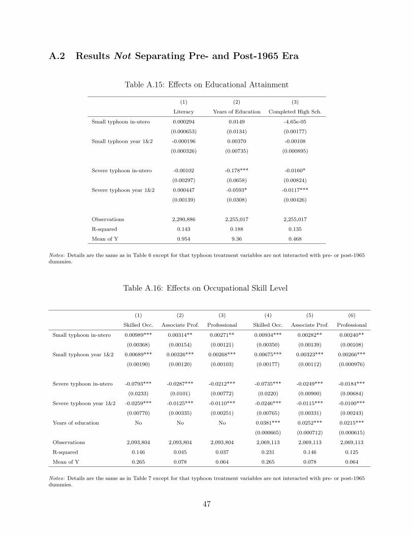
A.2 Results Not Separating Pre- and Post-1965 Era

Table A.15: Effects on Educational Attainment

(1) (2) (3)

Literacy Years of Education Completed High Sch.

Small typhoon in-utero 0.000294 0.0149 -4.65e-05

(0.000653) (0.0134) (0.00177)

Small typhoon year 1&2 -0.000196 0.00370 -0.00108

(0.000326) (0.00735) (0.000895)

Severe typhoon in-utero -0.00102 -0.178*** -0.0160*

(0.00297) (0.0658) (0.00824)

Severe typhoon year 1&2 0.000447 -0.0593* -0.0117***

(0.00139) (0.0308) (0.00426)

Observations 2,290,886 2,255,017 2,255,017

R-squared 0.143 0.188 0.135

Mean of Y 0.954 9.36 0.468

Notes: Details are the same as in Table 6 except for that typhoon treatment variables are not interacted with pre- or post-1965dummies.

Table A.16: Effects on Occupational Skill Level

(1) (2) (3) (4) (5) (6)

Skilled Occ. Associate Prof. Professional Skilled Occ. Associate Prof. Professional

Small typhoon in-utero 0.00989*** 0.00314** 0.00271** 0.00934*** 0.00282** 0.00240**

(0.00368) (0.00154) (0.00121) (0.00350) (0.00139) (0.00108)

Small typhoon year 1&2 0.00689*** 0.00326*** 0.00268*** 0.00675*** 0.00323*** 0.00266***

(0.00190) (0.00120) (0.00103) (0.00177) (0.00112) (0.000976)

Severe typhoon in-utero -0.0793*** -0.0287*** -0.0212*** -0.0735*** -0.0249*** -0.0184***

(0.0233) (0.0101) (0.00772) (0.0220) (0.00900) (0.00684)

Severe typhoon year 1&2 -0.0259*** -0.0125*** -0.0110*** -0.0246*** -0.0115*** -0.0100***

(0.00770) (0.00335) (0.00251) (0.00765) (0.00331) (0.00243)

Years of education No No No 0.0381*** 0.0252*** 0.0215***

(0.000665) (0.000712) (0.000615)

Observations 2,093,804 2,093,804 2,093,804 2,069,113 2,069,113 2,069,113

R-squared 0.146 0.045 0.037 0.231 0.146 0.125

Mean of Y 0.265 0.078 0.064 0.265 0.078 0.064

Notes: Details are the same as in Table 7 except for that typhoon treatment variables are not interacted with pre- or post-1965dummies.

47

Table A.17: Effects on Educational Attainment by Sex

(1) (2) (3) (4) (5) (6)

Literacy Years of Education Completed High Sch.

Male Female Male Female Male Female

Small typhoon in-utero 0.000369 0.000199 -0.00436 0.0356** -0.00155 0.00189

(0.000839) (0.000818) (0.0175) (0.0168) (0.00251) (0.00220)

Small typhoon year 1&2 -0.000131 -0.000296 0.00750 -9.95e-05 -0.000582 -0.00149

(0.000404) (0.000425) (0.00821) (0.00923) (0.00108) (0.00116)

Severe typhoon in-utero -0.00185 -0.000350 -0.199** -0.160** -0.0237** -0.00938

(0.00382) (0.00381) (0.0809) (0.0783) (0.0107) (0.00988)

Severe typhoon year 1&2 0.00113 -0.000411 -0.0563 -0.0655 -0.0130** -0.0109**

(0.00154) (0.00193) (0.0348) (0.0404) (0.00513) (0.00505)

Observations 1,144,609 1,146,277 1,127,900 1,127,117 1,127,900 1,127,117

R-squared 0.117 0.177 0.186 0.194 0.137 0.139

Mean of Y 0.955 0.954 9.20 9.51 0.458 0.479

Notes: Details are the same as in Table 8 except for that typhoon treatment variables are not interactedwith pre- or post-1965 dummies.

Table A.18: Effects on Occupational Skill Level by Sex

(1) (2) (3) (4) (5) (6)

Skilled Occupation Associate Professional Professional

Male Female Male Female Male Female

Small typhoon in-utero 0.0126** 0.00817** 0.00267 0.00363** 0.00213 0.00326**

(0.00492) (0.00333) (0.00191) (0.00165) (0.00149) (0.00143)

Small typhoon year 1&2 0.00687*** 0.00705*** 0.00325** 0.00328*** 0.00285** 0.00250**

(0.00233) (0.00194) (0.00141) (0.00115) (0.00119) (0.00102)

Severe typhoon in-utero -0.0878*** -0.0745*** -0.0351*** -0.0227** -0.0270*** -0.0157*

(0.0297) (0.0216) (0.0112) (0.0103) (0.00787) (0.00877)

Severe typhoon year 1&2 -0.0377*** -0.0164** -0.0144*** -0.0109*** -0.0114*** -0.0107***

(0.0105) (0.00642) (0.00463) (0.00307) (0.00344) (0.00255)

Years of education No No No No No No

Observations 1,043,359 1,050,445 1,043,359 1,050,445 1,043,359 1,050,445

R-squared 0.201 0.066 0.061 0.035 0.048 0.030

Mean of Y 0.339 0.191 0.076 0.080 0.058 0.070

Notes: Details are the same as in Table 9 except for that typhoon treatment variables are not interactedwith pre- or post-1965 dummies.

48

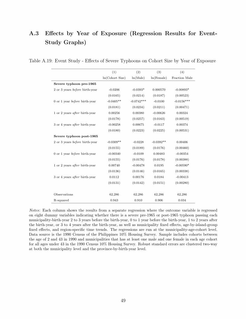
A.3 Effects by Year of Exposure (Regression Results for Event-

Study Graphs)

Table A.19: Event Study - Effects of Severe Typhoons on Cohort Size by Year of Exposure

(1) (2) (3) (4)

ln(Cohort Size) ln(Male) ln(Female) Fraction Male

Severe typhoon pre-1965

2 or 3 years before birth-year -0.0206 -0.0393* 0.000570 -0.00893*

(0.0165) (0.0214) (0.0187) (0.00523)

0 or 1 year before birth-year -0.0405** -0.0742*** -0.0100 -0.0156***

(0.0181) (0.0234) (0.0211) (0.00471)

1 or 2 years after birth-year 0.00256 0.00380 -0.00626 0.00324

(0.0178) (0.0257) (0.0163) (0.00519)

3 or 4 years after birth-year -0.00258 0.00675 -0.0117 0.00374

(0.0180) (0.0223) (0.0225) (0.00531)

Severe typhoon post-1965

2 or 3 years before birth-year -0.0309** -0.0228 -0.0392** 0.00406

(0.0155) (0.0189) (0.0176) (0.00460)

0 or 1 year before birth-year -0.00340 -0.0109 0.00483 -0.00354

(0.0155) (0.0176) (0.0178) (0.00388)

1 or 2 years after birth-year 0.00740 -0.00478 0.0195 -0.00590*

(0.0136) (0.0146) (0.0165) (0.00338)

3 or 4 years after birth-year 0.0112 0.00176 0.0184 -0.00413

(0.0131) (0.0142) (0.0151) (0.00280)

Observations 62,286 62,286 62,286 62,286

R-squared 0.943 0.910 0.906 0.034

Notes: Each column shows the results from a separate regression where the outcome variable is regressedon eight dummy variables indicating whether there is a severe pre-1965 or post-1965 typhoon passing eachmunicipality-birth-year 2 to 3 years before the birth-year, 0 to 1 year before the birth-year, 1 to 2 years afterthe birth-year, or 3 to 4 years after the birth-year, as well as municipality fixed effects, age-by-island-groupfixed effects, and region-specific time trends. The regressions are run at the municipality-age-cohort level.Data source is the 1990 Census of the Philippines 10% Housing Survey. Sample includes cohorts betweenthe age of 2 and 43 in 1990 and municipalities that has at least one male and one female in each age cohortfor all ages under 43 in the 1990 Census 10% Housing Survey. Robust standard errors are clustered two-wayat both the municipality level and the province-by-birth-year level.

49

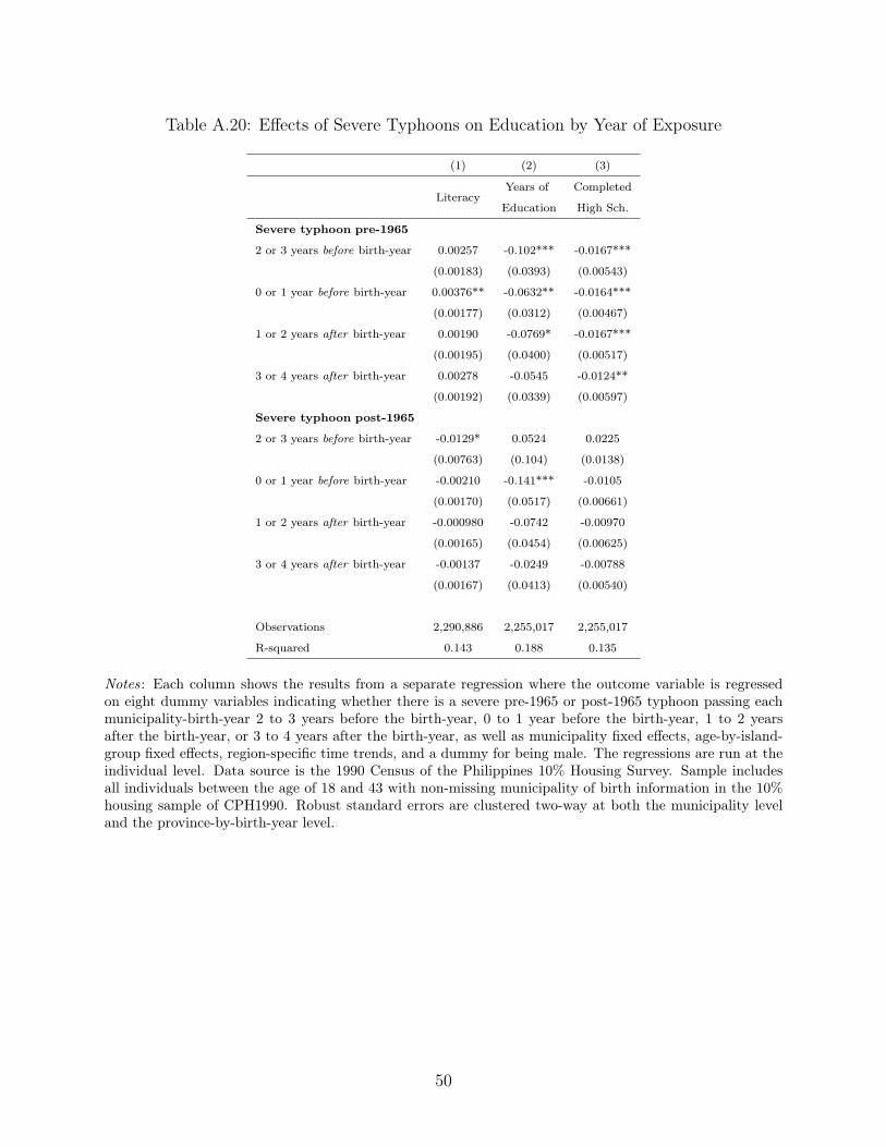
Table A.20: Effects of Severe Typhoons on Education by Year of Exposure

(1) (2) (3)

LiteracyYears of Completed

Education High Sch.

Severe typhoon pre-1965

2 or 3 years before birth-year 0.00257 -0.102*** -0.0167***

(0.00183) (0.0393) (0.00543)

0 or 1 year before birth-year 0.00376** -0.0632** -0.0164***

(0.00177) (0.0312) (0.00467)

1 or 2 years after birth-year 0.00190 -0.0769* -0.0167***

(0.00195) (0.0400) (0.00517)

3 or 4 years after birth-year 0.00278 -0.0545 -0.0124**

(0.00192) (0.0339) (0.00597)

Severe typhoon post-1965

2 or 3 years before birth-year -0.0129* 0.0524 0.0225

(0.00763) (0.104) (0.0138)

0 or 1 year before birth-year -0.00210 -0.141*** -0.0105

(0.00170) (0.0517) (0.00661)

1 or 2 years after birth-year -0.000980 -0.0742 -0.00970

(0.00165) (0.0454) (0.00625)

3 or 4 years after birth-year -0.00137 -0.0249 -0.00788

(0.00167) (0.0413) (0.00540)

Observations 2,290,886 2,255,017 2,255,017

R-squared 0.143 0.188 0.135

Notes: Each column shows the results from a separate regression where the outcome variable is regressedon eight dummy variables indicating whether there is a severe pre-1965 or post-1965 typhoon passing eachmunicipality-birth-year 2 to 3 years before the birth-year, 0 to 1 year before the birth-year, 1 to 2 yearsafter the birth-year, or 3 to 4 years after the birth-year, as well as municipality fixed effects, age-by-island-group fixed effects, region-specific time trends, and a dummy for being male. The regressions are run at theindividual level. Data source is the 1990 Census of the Philippines 10% Housing Survey. Sample includesall individuals between the age of 18 and 43 with non-missing municipality of birth information in the 10%housing sample of CPH1990. Robust standard errors are clustered two-way at both the municipality leveland the province-by-birth-year level.

50

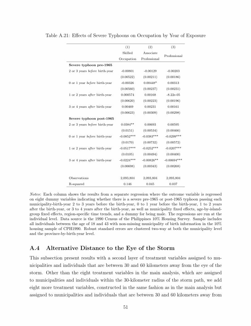
Table A.21: Effects of Severe Typhoons on Occupation by Year of Exposure

(1) (2) (3)

Skilled AssociateProfessional

Occupation Professional

Severe typhoon pre-1965

2 or 3 years before birth-year -0.00801 -0.00129 -0.00203

(0.00522) (0.00211) (0.00186)

0 or 1 year before birth-year -0.00326 0.00448* 0.00313

(0.00560) (0.00237) (0.00231)

1 or 2 years after birth-year 0.000574 0.00168 -8.22e-05

(0.00620) (0.00223) (0.00196)

3 or 4 years after birth-year 0.00469 0.00231 0.00161

(0.00623) (0.00309) (0.00298)

Severe typhoon post-1965

2 or 3 years before birth-year 0.0384** 0.00693 0.00595

(0.0151) (0.00534) (0.00466)

0 or 1 year before birth-year -0.0852*** -0.0383*** -0.0299***

(0.0170) (0.00732) (0.00572)

1 or 2 years after birth-year -0.0517*** -0.0252*** -0.0207***

(0.0105) (0.00494) (0.00400)

3 or 4 years after birth-year -0.0224*** -0.00826** -0.00694***

(0.00698) (0.00343) (0.00268)

Observations 2,093,804 2,093,804 2,093,804

R-squared 0.146 0.045 0.037

Notes: Each column shows the results from a separate regression where the outcome variable is regressedon eight dummy variables indicating whether there is a severe pre-1965 or post-1965 typhoon passing eachmunicipality-birth-year 2 to 3 years before the birth-year, 0 to 1 year before the birth-year, 1 to 2 yearsafter the birth-year, or 3 to 4 years after the birth-year, as well as municipality fixed effects, age-by-island-group fixed effects, region-specific time trends, and a dummy for being male. The regressions are run at theindividual level. Data source is the 1990 Census of the Philippines 10% Housing Survey. Sample includesall individuals between the age of 18 and 43 with non-missing municipality of birth information in the 10%housing sample of CPH1990. Robust standard errors are clustered two-way at both the municipality leveland the province-by-birth-year level.

A.4 Alternative Distance to the Eye of the Storm

This subsection present results with a second layer of treatment variables assigned to mu-nicipalities and individuals that are between 30 and 60 kilometers away from the eye of thestorm. Other than the eight treatment variables in the main analysis, which are assignedto municipalities and individuals within the 30-kilometer radius of the storm path, we addeight more treatment variables, constructed in the same fashion as in the main analysis butassigned to municipalities and individuals that are between 30 and 60 kilometers away from

51

the eye of the storm. Specifically, a municipality is exposed to a typhoon 30 to 60 kilometersaway if the distance between the centroid of the municipality and the typhoon path is largerthan 30km but no larger than 60km.

As such, we estimate the effects of typhoon exposure on municipalities and individualswithin 30 kilometers of the typhoon path as well as municipalities and individuals between30 and 60 kilometers away from the typhoon path. The “control group” here is, thus, mu-nicipalities and individuals outside of the 60-kilometer radius of the storm path.

Tables A.22 and A.23 present results for cohort size and fraction of male. Tables A.24 andA.25 present results for educational attainment and occupational skill levels, respectively.Tables A.26 and A.27 seperately estimate the long-term outcomes by sex.

52

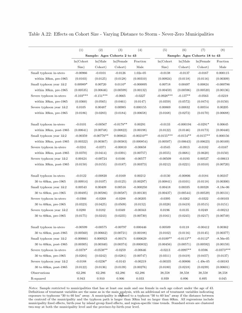
Table A.22: Effects on Cohort Size - Varying Distance to Storm - Never-Zero Municipalities

(1) (2) (3) (4) (5) (6) (7) (8)

Sample: Ages Cohorts 2 to 43 Sample: Ages Cohorts 18 to 43

ln(Cohort ln(Male ln(Female Fraction ln(Cohort ln(Male ln(Female Fraction

Size) Cohort) Cohort) Male Size) Cohort) Cohort) Male

Small typhoon in-utero -0.00966 -0.0101 -0.0126 1.02e-05 -0.0138 -0.0137 -0.0167 0.000115

within 30km, pre-1965 (0.0103) (0.0125) (0.0128) (0.00310) (0.00924) (0.0118) (0.0116) (0.00309)

Small typhoon year 1&2 0.00989* 0.00720 0.0110* -0.000895 0.00718 0.00497 0.00824 -0.000786

within 30km, pre-1965 (0.00535) (0.00646) (0.00599) (0.00132) (0.00459) (0.00596) (0.00520) (0.00136)

Severe typhoon in-utero -0.103*** -0.151*** -0.0665 -0.0227 -0.0928*** -0.137** -0.0563 -0.0219

within 30km, pre-1965 (0.0360) (0.0565) (0.0461) (0.0147) (0.0359) (0.0572) (0.0474) (0.0150)

Severe typhoon year 1&2 0.0105 0.00487 0.00985 0.000155 0.00869 0.00832 0.00554 0.00205

within 30km, pre-1965 (0.0186) (0.0283) (0.0184) (0.00658) (0.0168) (0.0272) (0.0170) (0.00688)

Small typhoon in-utero -0.0101 -0.00567 -0.0178** 0.00291 -0.0133 -0.000194 -0.0291* 0.00645

within 30km, post-1965 (0.00641) (0.00748) (0.00822) (0.00198) (0.0122) (0.0146) (0.0173) (0.00440)

Small typhoon year 1&2 -0.00359 -0.00776** 0.000621 -0.00210** -0.0155*** -0.0154** -0.0157** 0.000156

within 30km, post-1965 (0.00322) (0.00367) (0.00383) (0.000854) (0.00507) (0.00643) (0.00623) (0.00169)

Severe typhoon in-utero -0.0241 -0.0371 -0.00810 -0.00658 -0.0545 -0.0913 -0.0182 -0.0167

within 30km, post-1965 (0.0370) (0.0414) (0.0391) (0.00757) (0.0555) (0.0681) (0.0620) (0.0150)

Severe typhoon year 1&2 0.00424 -0.00724 0.0166 -0.00577 -0.00509 -0.0193 0.00527 -0.00613

within 30km, post-1965 (0.0150) (0.0155) (0.0187) (0.00373) (0.0212) (0.0221) (0.0310) (0.00720)

Small typhoon in-utero -0.0122 -0.00820 -0.0169 0.00212 -0.0130 -0.00806 -0.0184 0.00247

30 to 60km, pre-1965 (0.00914) (0.0107) (0.0125) (0.00297) (0.00841) (0.0101) (0.0118) (0.00300)

Small typhoon year 1&2 0.00543 0.00409 0.00516 -0.000250 0.00418 0.00335 0.00328 -8.18e-06

30 to 60km, pre-1965 (0.00495) (0.00586) (0.00587) (0.00130) (0.00437) (0.00544) (0.00529) (0.00131)

Severe typhoon in-utero -0.0366 -0.0268 -0.0288 -0.00205 -0.0395 -0.0262 -0.0322 -0.00103

30 to 60km, pre-1965 (0.0323) (0.0425) (0.0509) (0.0152) (0.0328) (0.0419) (0.0515) (0.0151)

Severe typhoon year 1&2 0.0280 0.0182 0.0349 -0.00343 0.0196 0.0135 0.0249 -0.00212

30 to 60km, pre-1965 (0.0175) (0.0243) (0.0235) (0.00730) (0.0161) (0.0245) (0.0217) (0.00749)

Small typhoon in-utero -0.00599 -0.00575 -0.00797 0.000446 0.00509 0.0118 -0.00412 0.00362

30 to 60km, post-1965 (0.00560) (0.00662) (0.00721) (0.00188) (0.0102) (0.0116) (0.0145) (0.00377)

Small typhoon year 1&2 -0.000661 0.000923 -0.00174 0.000629 -0.0109** -0.0113** -0.0112* -8.56e-05

30 to 60km, post-1965 (0.00305) (0.00340) (0.00374) (0.000832) (0.00456) (0.00571) (0.00592) (0.00159)

Severe typhoon in-utero -0.0378* -0.0538** -0.0259 -0.00646 -0.0213 -0.0997** 0.0596 -0.0373***

30 to 60km, pre-1965 (0.0204) (0.0242) (0.0281) (0.00747) (0.0311) (0.0419) (0.0457) (0.0137)

Severe typhoon year 1&2 -0.0188 -0.0236* -0.0143 -0.00219 -0.00335 -0.00806 -1.49e-05 -0.00183

30 to 60km, post-1965 (0.0122) (0.0136) (0.0139) (0.00276) (0.0180) (0.0218) (0.0239) (0.00601)

Observations 62,286 62,286 62,286 62,286 38,558 38,558 38,558 38,558

R-squared 0.943 0.910 0.906 0.033 0.939 0.896 0.895 0.045

Notes: Sample restricted to municipalities that has at least one male and one female in each age cohort under the age of 43.Definitions of treatment variables are the same as in the main analysis, with an additional set of treatment variables indicatingexposure to typhoons “30 to 60 km” away. A municipality is exposed to a typhoon “30 to 60 km” away if the distance betweenthe centroid of the municipality and the typhoon path is larger than 30km but no larger than 60km. All regressions includemunicipality fixed effects, birth-year by island group fixed effects, and region-specific time trends. Standard errors are clusteredtwo-way at both the municipality level and the province-by-birth-year level.

53

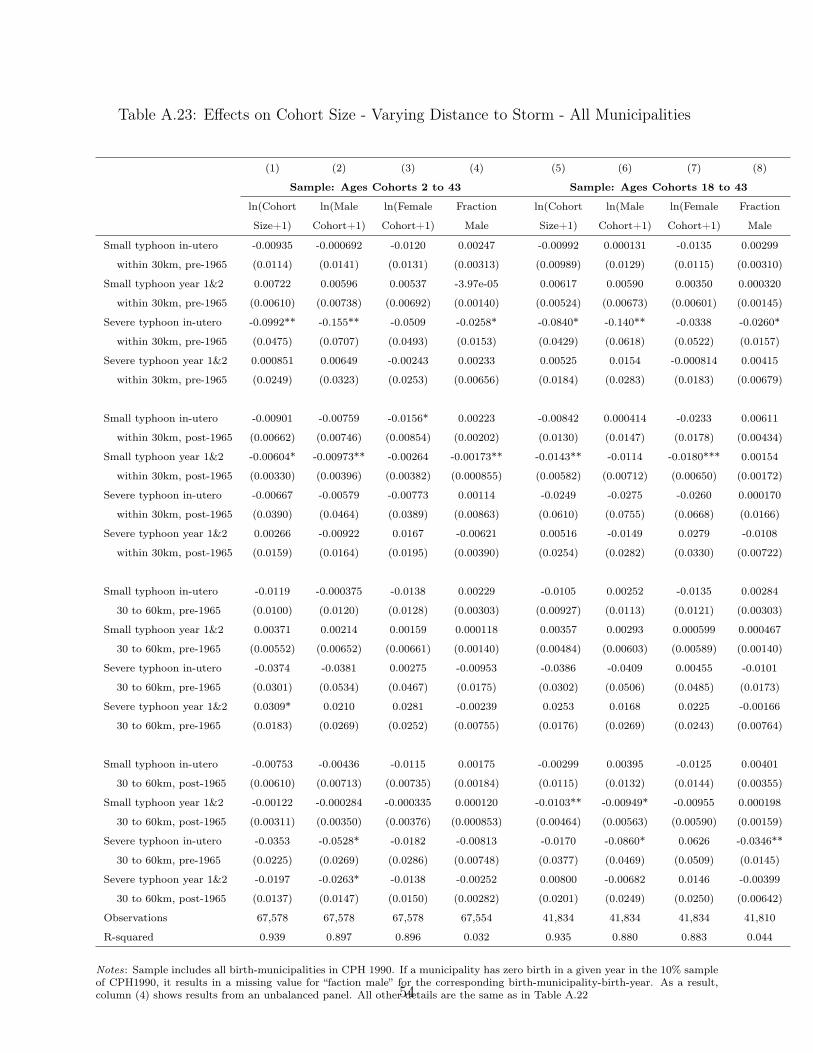
Table A.23: Effects on Cohort Size - Varying Distance to Storm - All Municipalities

(1) (2) (3) (4) (5) (6) (7) (8)

Sample: Ages Cohorts 2 to 43 Sample: Ages Cohorts 18 to 43

ln(Cohort ln(Male ln(Female Fraction ln(Cohort ln(Male ln(Female Fraction

Size+1) Cohort+1) Cohort+1) Male Size+1) Cohort+1) Cohort+1) Male

Small typhoon in-utero -0.00935 -0.000692 -0.0120 0.00247 -0.00992 0.000131 -0.0135 0.00299

within 30km, pre-1965 (0.0114) (0.0141) (0.0131) (0.00313) (0.00989) (0.0129) (0.0115) (0.00310)

Small typhoon year 1&2 0.00722 0.00596 0.00537 -3.97e-05 0.00617 0.00590 0.00350 0.000320

within 30km, pre-1965 (0.00610) (0.00738) (0.00692) (0.00140) (0.00524) (0.00673) (0.00601) (0.00145)

Severe typhoon in-utero -0.0992** -0.155** -0.0509 -0.0258* -0.0840* -0.140** -0.0338 -0.0260*

within 30km, pre-1965 (0.0475) (0.0707) (0.0493) (0.0153) (0.0429) (0.0618) (0.0522) (0.0157)

Severe typhoon year 1&2 0.000851 0.00649 -0.00243 0.00233 0.00525 0.0154 -0.000814 0.00415

within 30km, pre-1965 (0.0249) (0.0323) (0.0253) (0.00656) (0.0184) (0.0283) (0.0183) (0.00679)

Small typhoon in-utero -0.00901 -0.00759 -0.0156* 0.00223 -0.00842 0.000414 -0.0233 0.00611

within 30km, post-1965 (0.00662) (0.00746) (0.00854) (0.00202) (0.0130) (0.0147) (0.0178) (0.00434)

Small typhoon year 1&2 -0.00604* -0.00973** -0.00264 -0.00173** -0.0143** -0.0114 -0.0180*** 0.00154

within 30km, post-1965 (0.00330) (0.00396) (0.00382) (0.000855) (0.00582) (0.00712) (0.00650) (0.00172)

Severe typhoon in-utero -0.00667 -0.00579 -0.00773 0.00114 -0.0249 -0.0275 -0.0260 0.000170

within 30km, post-1965 (0.0390) (0.0464) (0.0389) (0.00863) (0.0610) (0.0755) (0.0668) (0.0166)

Severe typhoon year 1&2 0.00266 -0.00922 0.0167 -0.00621 0.00516 -0.0149 0.0279 -0.0108

within 30km, post-1965 (0.0159) (0.0164) (0.0195) (0.00390) (0.0254) (0.0282) (0.0330) (0.00722)

Small typhoon in-utero -0.0119 -0.000375 -0.0138 0.00229 -0.0105 0.00252 -0.0135 0.00284

30 to 60km, pre-1965 (0.0100) (0.0120) (0.0128) (0.00303) (0.00927) (0.0113) (0.0121) (0.00303)

Small typhoon year 1&2 0.00371 0.00214 0.00159 0.000118 0.00357 0.00293 0.000599 0.000467

30 to 60km, pre-1965 (0.00552) (0.00652) (0.00661) (0.00140) (0.00484) (0.00603) (0.00589) (0.00140)

Severe typhoon in-utero -0.0374 -0.0381 0.00275 -0.00953 -0.0386 -0.0409 0.00455 -0.0101

30 to 60km, pre-1965 (0.0301) (0.0534) (0.0467) (0.0175) (0.0302) (0.0506) (0.0485) (0.0173)

Severe typhoon year 1&2 0.0309* 0.0210 0.0281 -0.00239 0.0253 0.0168 0.0225 -0.00166

30 to 60km, pre-1965 (0.0183) (0.0269) (0.0252) (0.00755) (0.0176) (0.0269) (0.0243) (0.00764)

Small typhoon in-utero -0.00753 -0.00436 -0.0115 0.00175 -0.00299 0.00395 -0.0125 0.00401

30 to 60km, post-1965 (0.00610) (0.00713) (0.00735) (0.00184) (0.0115) (0.0132) (0.0144) (0.00355)

Small typhoon year 1&2 -0.00122 -0.000284 -0.000335 0.000120 -0.0103** -0.00949* -0.00955 0.000198

30 to 60km, post-1965 (0.00311) (0.00350) (0.00376) (0.000853) (0.00464) (0.00563) (0.00590) (0.00159)

Severe typhoon in-utero -0.0353 -0.0528* -0.0182 -0.00813 -0.0170 -0.0860* 0.0626 -0.0346**

30 to 60km, pre-1965 (0.0225) (0.0269) (0.0286) (0.00748) (0.0377) (0.0469) (0.0509) (0.0145)

Severe typhoon year 1&2 -0.0197 -0.0263* -0.0138 -0.00252 0.00800 -0.00682 0.0146 -0.00399

30 to 60km, post-1965 (0.0137) (0.0147) (0.0150) (0.00282) (0.0201) (0.0249) (0.0250) (0.00642)

Observations 67,578 67,578 67,578 67,554 41,834 41,834 41,834 41,810

R-squared 0.939 0.897 0.896 0.032 0.935 0.880 0.883 0.044

Notes: Sample includes all birth-municipalities in CPH 1990. If a municipality has zero birth in a given year in the 10% sampleof CPH1990, it results in a missing value for “faction male” for the corresponding birth-municipality-birth-year. As a result,column (4) shows results from an unbalanced panel. All other details are the same as in Table A.2254

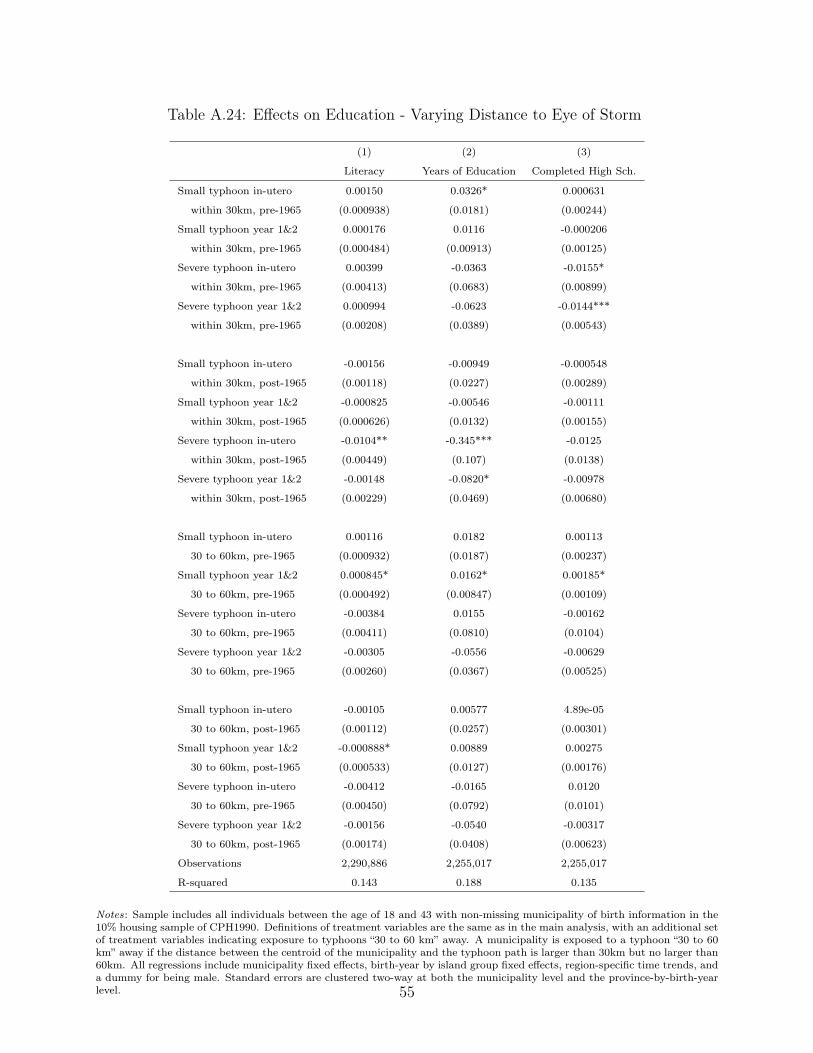
Table A.24: Effects on Education - Varying Distance to Eye of Storm

(1) (2) (3)

Literacy Years of Education Completed High Sch.

Small typhoon in-utero 0.00150 0.0326* 0.000631

within 30km, pre-1965 (0.000938) (0.0181) (0.00244)

Small typhoon year 1&2 0.000176 0.0116 -0.000206

within 30km, pre-1965 (0.000484) (0.00913) (0.00125)

Severe typhoon in-utero 0.00399 -0.0363 -0.0155*

within 30km, pre-1965 (0.00413) (0.0683) (0.00899)

Severe typhoon year 1&2 0.000994 -0.0623 -0.0144***

within 30km, pre-1965 (0.00208) (0.0389) (0.00543)

Small typhoon in-utero -0.00156 -0.00949 -0.000548

within 30km, post-1965 (0.00118) (0.0227) (0.00289)

Small typhoon year 1&2 -0.000825 -0.00546 -0.00111

within 30km, post-1965 (0.000626) (0.0132) (0.00155)

Severe typhoon in-utero -0.0104** -0.345*** -0.0125

within 30km, post-1965 (0.00449) (0.107) (0.0138)

Severe typhoon year 1&2 -0.00148 -0.0820* -0.00978

within 30km, post-1965 (0.00229) (0.0469) (0.00680)

Small typhoon in-utero 0.00116 0.0182 0.00113

30 to 60km, pre-1965 (0.000932) (0.0187) (0.00237)

Small typhoon year 1&2 0.000845* 0.0162* 0.00185*

30 to 60km, pre-1965 (0.000492) (0.00847) (0.00109)

Severe typhoon in-utero -0.00384 0.0155 -0.00162

30 to 60km, pre-1965 (0.00411) (0.0810) (0.0104)

Severe typhoon year 1&2 -0.00305 -0.0556 -0.00629

30 to 60km, pre-1965 (0.00260) (0.0367) (0.00525)

Small typhoon in-utero -0.00105 0.00577 4.89e-05

30 to 60km, post-1965 (0.00112) (0.0257) (0.00301)

Small typhoon year 1&2 -0.000888* 0.00889 0.00275

30 to 60km, post-1965 (0.000533) (0.0127) (0.00176)

Severe typhoon in-utero -0.00412 -0.0165 0.0120

30 to 60km, pre-1965 (0.00450) (0.0792) (0.0101)

Severe typhoon year 1&2 -0.00156 -0.0540 -0.00317

30 to 60km, post-1965 (0.00174) (0.0408) (0.00623)

Observations 2,290,886 2,255,017 2,255,017

R-squared 0.143 0.188 0.135

Notes: Sample includes all individuals between the age of 18 and 43 with non-missing municipality of birth information in the10% housing sample of CPH1990. Definitions of treatment variables are the same as in the main analysis, with an additional setof treatment variables indicating exposure to typhoons “30 to 60 km” away. A municipality is exposed to a typhoon “30 to 60km” away if the distance between the centroid of the municipality and the typhoon path is larger than 30km but no larger than60km. All regressions include municipality fixed effects, birth-year by island group fixed effects, region-specific time trends, anda dummy for being male. Standard errors are clustered two-way at both the municipality level and the province-by-birth-yearlevel. 55

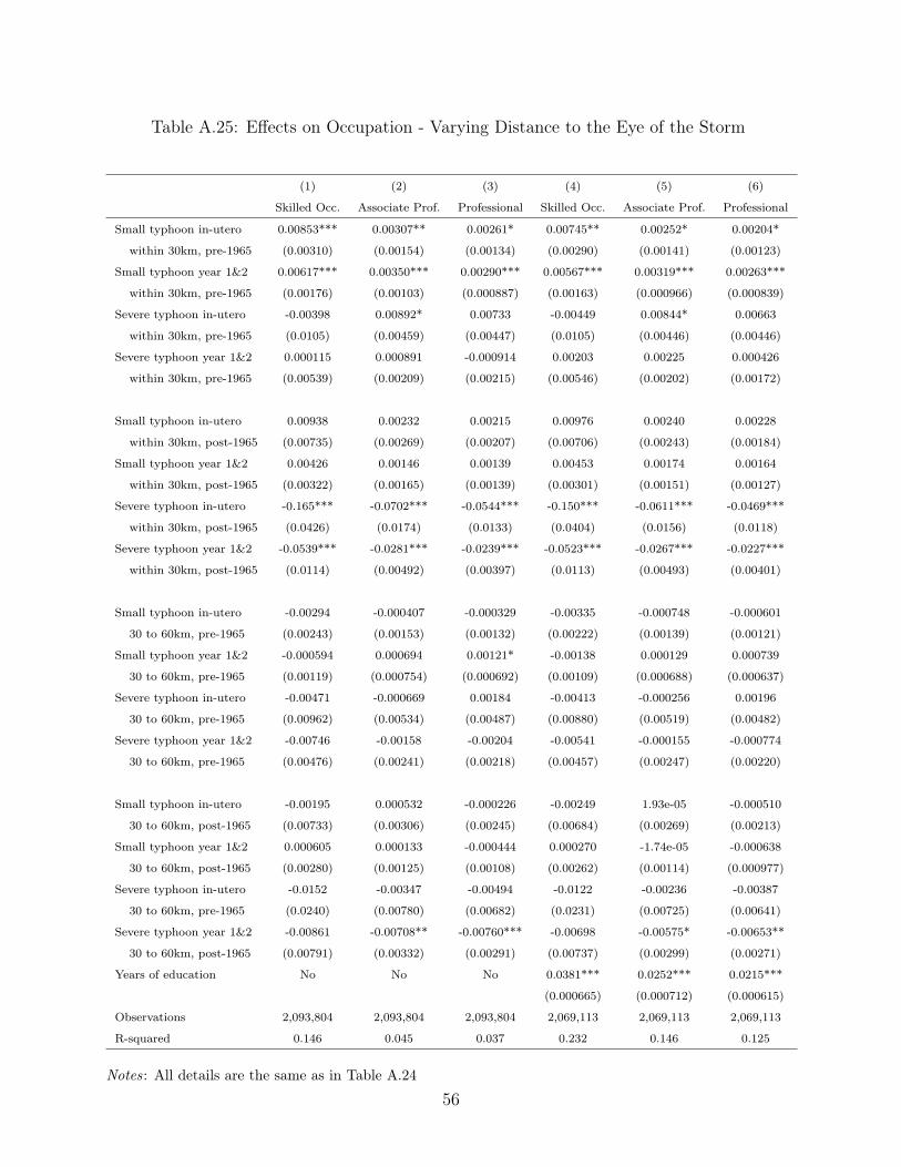
Table A.25: Effects on Occupation - Varying Distance to the Eye of the Storm

(1) (2) (3) (4) (5) (6)

Skilled Occ. Associate Prof. Professional Skilled Occ. Associate Prof. Professional

Small typhoon in-utero 0.00853*** 0.00307** 0.00261* 0.00745** 0.00252* 0.00204*

within 30km, pre-1965 (0.00310) (0.00154) (0.00134) (0.00290) (0.00141) (0.00123)

Small typhoon year 1&2 0.00617*** 0.00350*** 0.00290*** 0.00567*** 0.00319*** 0.00263***

within 30km, pre-1965 (0.00176) (0.00103) (0.000887) (0.00163) (0.000966) (0.000839)

Severe typhoon in-utero -0.00398 0.00892* 0.00733 -0.00449 0.00844* 0.00663

within 30km, pre-1965 (0.0105) (0.00459) (0.00447) (0.0105) (0.00446) (0.00446)

Severe typhoon year 1&2 0.000115 0.000891 -0.000914 0.00203 0.00225 0.000426

within 30km, pre-1965 (0.00539) (0.00209) (0.00215) (0.00546) (0.00202) (0.00172)

Small typhoon in-utero 0.00938 0.00232 0.00215 0.00976 0.00240 0.00228

within 30km, post-1965 (0.00735) (0.00269) (0.00207) (0.00706) (0.00243) (0.00184)

Small typhoon year 1&2 0.00426 0.00146 0.00139 0.00453 0.00174 0.00164

within 30km, post-1965 (0.00322) (0.00165) (0.00139) (0.00301) (0.00151) (0.00127)

Severe typhoon in-utero -0.165*** -0.0702*** -0.0544*** -0.150*** -0.0611*** -0.0469***

within 30km, post-1965 (0.0426) (0.0174) (0.0133) (0.0404) (0.0156) (0.0118)

Severe typhoon year 1&2 -0.0539*** -0.0281*** -0.0239*** -0.0523*** -0.0267*** -0.0227***

within 30km, post-1965 (0.0114) (0.00492) (0.00397) (0.0113) (0.00493) (0.00401)

Small typhoon in-utero -0.00294 -0.000407 -0.000329 -0.00335 -0.000748 -0.000601

30 to 60km, pre-1965 (0.00243) (0.00153) (0.00132) (0.00222) (0.00139) (0.00121)

Small typhoon year 1&2 -0.000594 0.000694 0.00121* -0.00138 0.000129 0.000739

30 to 60km, pre-1965 (0.00119) (0.000754) (0.000692) (0.00109) (0.000688) (0.000637)

Severe typhoon in-utero -0.00471 -0.000669 0.00184 -0.00413 -0.000256 0.00196

30 to 60km, pre-1965 (0.00962) (0.00534) (0.00487) (0.00880) (0.00519) (0.00482)

Severe typhoon year 1&2 -0.00746 -0.00158 -0.00204 -0.00541 -0.000155 -0.000774

30 to 60km, pre-1965 (0.00476) (0.00241) (0.00218) (0.00457) (0.00247) (0.00220)

Small typhoon in-utero -0.00195 0.000532 -0.000226 -0.00249 1.93e-05 -0.000510

30 to 60km, post-1965 (0.00733) (0.00306) (0.00245) (0.00684) (0.00269) (0.00213)

Small typhoon year 1&2 0.000605 0.000133 -0.000444 0.000270 -1.74e-05 -0.000638

30 to 60km, post-1965 (0.00280) (0.00125) (0.00108) (0.00262) (0.00114) (0.000977)

Severe typhoon in-utero -0.0152 -0.00347 -0.00494 -0.0122 -0.00236 -0.00387

30 to 60km, pre-1965 (0.0240) (0.00780) (0.00682) (0.0231) (0.00725) (0.00641)

Severe typhoon year 1&2 -0.00861 -0.00708** -0.00760*** -0.00698 -0.00575* -0.00653**

30 to 60km, post-1965 (0.00791) (0.00332) (0.00291) (0.00737) (0.00299) (0.00271)

Years of education No No No 0.0381*** 0.0252*** 0.0215***

(0.000665) (0.000712) (0.000615)

Observations 2,093,804 2,093,804 2,093,804 2,069,113 2,069,113 2,069,113

R-squared 0.146 0.045 0.037 0.232 0.146 0.125

Notes: All details are the same as in Table A.24

56

Table A.26: Effects on Education by Sex - Varying Distance to Storm

(1) (2) (3) (4) (5) (6)

Literacy Years of Education Completed High Sch.

Male Female Male Female Male Female

Small typhoon in-utero 0.00115 0.00181 0.0146 0.0526** 0.000102 0.00145

within 30km, pre-1965 (0.00113) (0.00127) (0.0240) (0.0230) (0.00328) (0.00308)

Small typhoon year 1&2 0.000126 0.000214 0.00957 0.0135 -0.000245 -0.000164

within 30km, pre-1965 (0.000577) (0.000636) (0.0108) (0.0119) (0.00152) (0.00160)

Severe typhoon in-utero 0.00355 0.00425 -0.0136 -0.0611 -0.0226* -0.00805

within 30km, pre-1965 (0.00527) (0.00567) (0.103) (0.0866) (0.0126) (0.0107)

Severe typhoon year 1&2 0.00131 0.000373 -0.0442 -0.0818* -0.0179** -0.0107*

within 30km, pre-1965 (0.00253) (0.00320) (0.0575) (0.0483) (0.00782) (0.00576)

Small typhoon in-utero -0.000977 -0.00222 -0.0251 0.00734 -0.00225 0.00195

within 30km, post-1965 (0.00142) (0.00148) (0.0256) (0.0302) (0.00390) (0.00364)

Small typhoon year 1&2 -0.000701 -0.00105 0.00516 -0.0163 0.000537 -0.00268

within 30km, post-1965 (0.000698) (0.000807) (0.0133) (0.0163) (0.00185) (0.00198)

Severe typhoon in-utero -0.0114** -0.00997* -0.390*** -0.308** -0.0140 -0.0145

within 30km, post-1965 (0.00518) (0.00581) (0.111) (0.131) (0.0178) (0.0166)

Severe typhoon year 1&2 0.000132 -0.00320 -0.0675 -0.104* -0.00684 -0.0141

within 30km, post-1965 (0.00233) (0.00284) (0.0500) (0.0624) (0.00773) (0.00865)

Small typhoon in-utero 0.000905 0.00134 0.0328 0.00551 0.00446 -0.00200

30 to 60km, pre-1965 (0.00117) (0.00123) (0.0234) (0.0241) (0.00303) (0.00305)

Small typhoon year 1&2 0.000276 0.00138** 0.00908 0.0224** 0.00183 0.00167

30 to 60km, pre-1965 (0.000577) (0.000640) (0.0108) (0.0110) (0.00140) (0.00140)

Severe typhoon in-utero -0.00866 0.000158 -0.0664 0.0839 -0.0115 0.00685

30 to 60km, pre-1965 (0.00793) (0.00505) (0.122) (0.0919) (0.0152) (0.0140)

Severe typhoon year 1&2 -0.00494 -0.00107 -0.0823 -0.0310 -0.0102 -0.00265

30 to 60km, pre-1965 (0.00364) (0.00392) (0.0569) (0.0451) (0.00784) (0.00596)

Small typhoon in-utero -0.000161 -0.00205 0.0465 -0.0326 0.00769* -0.00698*

30 to 60km, post-1965 (0.00124) (0.00150) (0.0283) (0.0323) (0.00405) (0.00376)

Small typhoon year 1&2 -0.000428 -0.00144** 0.0151 0.00206 0.00251 0.00300

30 to 60km, post-1965 (0.000628) (0.000693) (0.0136) (0.0151) (0.00202) (0.00205)

Severe typhoon in-utero -0.00600 -0.00281 -0.0418 -0.00842 0.0215 -0.000294

30 to 60km, pre-1965 (0.00449) (0.00598) (0.0859) (0.0958) (0.0133) (0.0129)

Severe typhoon year 1&2 0.000178 -0.00327 0.0115 -0.123*** 0.00397 -0.0111

30 to 60km, post-1965 (0.00233) (0.00216) (0.0560) (0.0420) (0.00844) (0.00710)

Observations 1,144,609 1,146,277 1,127,900 1,127,117 1,127,900 1,127,117

R-squared 0.117 0.177 0.186 0.194 0.137 0.139

Notes: Each column is a separate regression using the sub-sample of either male or female correspondents in the CPH199010% sample. All regressions include municipality fixed effects, birth-year-by-island-group fixed effects, and region-specific timetrends. Standard errors are clustered two-way at both the municipality level and the province-by-birth-year level.

57

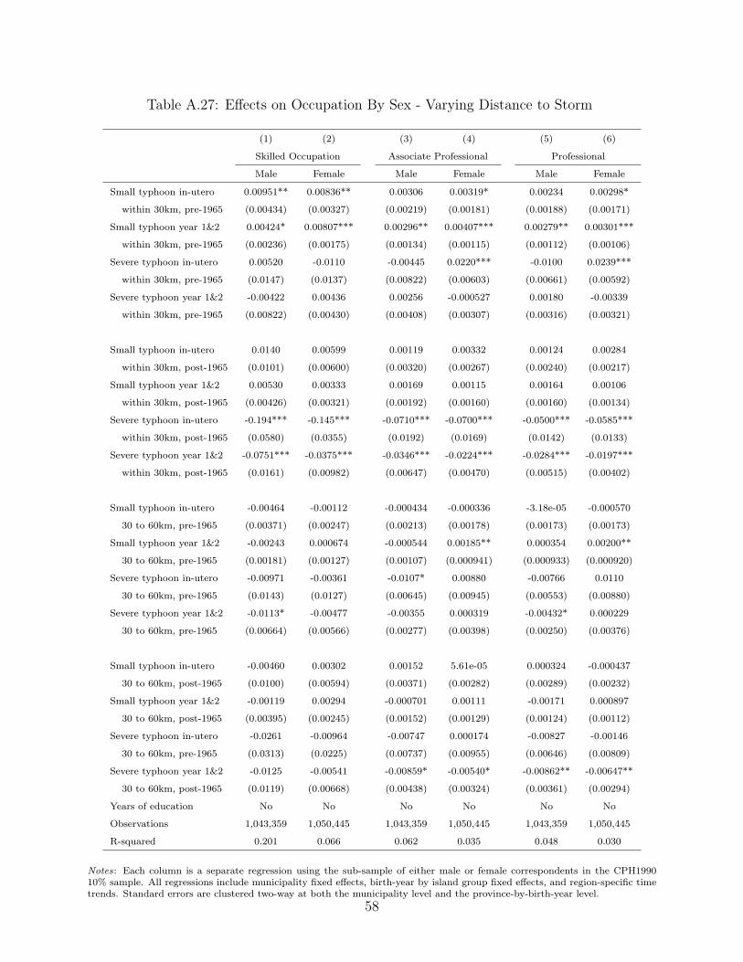
Table A.27: Effects on Occupation By Sex - Varying Distance to Storm

(1) (2) (3) (4) (5) (6)

Skilled Occupation Associate Professional Professional

Male Female Male Female Male Female

Small typhoon in-utero 0.00951** 0.00836** 0.00306 0.00319* 0.00234 0.00298*

within 30km, pre-1965 (0.00434) (0.00327) (0.00219) (0.00181) (0.00188) (0.00171)

Small typhoon year 1&2 0.00424* 0.00807*** 0.00296** 0.00407*** 0.00279** 0.00301***

within 30km, pre-1965 (0.00236) (0.00175) (0.00134) (0.00115) (0.00112) (0.00106)

Severe typhoon in-utero 0.00520 -0.0110 -0.00445 0.0220*** -0.0100 0.0239***

within 30km, pre-1965 (0.0147) (0.0137) (0.00822) (0.00603) (0.00661) (0.00592)

Severe typhoon year 1&2 -0.00422 0.00436 0.00256 -0.000527 0.00180 -0.00339

within 30km, pre-1965 (0.00822) (0.00430) (0.00408) (0.00307) (0.00316) (0.00321)

Small typhoon in-utero 0.0140 0.00599 0.00119 0.00332 0.00124 0.00284

within 30km, post-1965 (0.0101) (0.00600) (0.00320) (0.00267) (0.00240) (0.00217)

Small typhoon year 1&2 0.00530 0.00333 0.00169 0.00115 0.00164 0.00106

within 30km, post-1965 (0.00426) (0.00321) (0.00192) (0.00160) (0.00160) (0.00134)

Severe typhoon in-utero -0.194*** -0.145*** -0.0710*** -0.0700*** -0.0500*** -0.0585***

within 30km, post-1965 (0.0580) (0.0355) (0.0192) (0.0169) (0.0142) (0.0133)

Severe typhoon year 1&2 -0.0751*** -0.0375*** -0.0346*** -0.0224*** -0.0284*** -0.0197***

within 30km, post-1965 (0.0161) (0.00982) (0.00647) (0.00470) (0.00515) (0.00402)

Small typhoon in-utero -0.00464 -0.00112 -0.000434 -0.000336 -3.18e-05 -0.000570

30 to 60km, pre-1965 (0.00371) (0.00247) (0.00213) (0.00178) (0.00173) (0.00173)

Small typhoon year 1&2 -0.00243 0.000674 -0.000544 0.00185** 0.000354 0.00200**

30 to 60km, pre-1965 (0.00181) (0.00127) (0.00107) (0.000941) (0.000933) (0.000920)

Severe typhoon in-utero -0.00971 -0.00361 -0.0107* 0.00880 -0.00766 0.0110

30 to 60km, pre-1965 (0.0143) (0.0127) (0.00645) (0.00945) (0.00553) (0.00880)

Severe typhoon year 1&2 -0.0113* -0.00477 -0.00355 0.000319 -0.00432* 0.000229

30 to 60km, pre-1965 (0.00664) (0.00566) (0.00277) (0.00398) (0.00250) (0.00376)

Small typhoon in-utero -0.00460 0.00302 0.00152 5.61e-05 0.000324 -0.000437

30 to 60km, post-1965 (0.0100) (0.00594) (0.00371) (0.00282) (0.00289) (0.00232)

Small typhoon year 1&2 -0.00119 0.00294 -0.000701 0.00111 -0.00171 0.000897

30 to 60km, post-1965 (0.00395) (0.00245) (0.00152) (0.00129) (0.00124) (0.00112)

Severe typhoon in-utero -0.0261 -0.00964 -0.00747 0.000174 -0.00827 -0.00146

30 to 60km, pre-1965 (0.0313) (0.0225) (0.00737) (0.00955) (0.00646) (0.00809)

Severe typhoon year 1&2 -0.0125 -0.00541 -0.00859* -0.00540* -0.00862** -0.00647**

30 to 60km, post-1965 (0.0119) (0.00668) (0.00438) (0.00324) (0.00361) (0.00294)

Years of education No No No No No No

Observations 1,043,359 1,050,445 1,043,359 1,050,445 1,043,359 1,050,445

R-squared 0.201 0.066 0.062 0.035 0.048 0.030

Notes: Each column is a separate regression using the sub-sample of either male or female correspondents in the CPH199010% sample. All regressions include municipality fixed effects, birth-year by island group fixed effects, and region-specific timetrends. Standard errors are clustered two-way at both the municipality level and the province-by-birth-year level.

58

A.5 Alternative Storm Intensity Measures

In this subsection, we separately estimate the effects for each Saffir-Simpson storm scale.Instead of using two storm intensity categories (small and severe), we now allow four differentstorm intensity categories. We continue to combine SS scale 4 and scale 5 storms in onecategory because only a small number of municipalities were ever exposed to scale 5 storms.

59

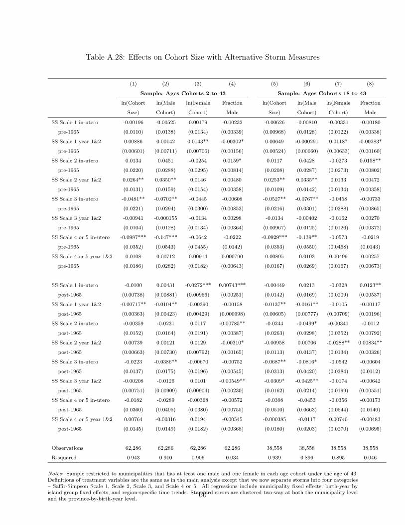
Table A.28: Effects on Cohort Size with Alternative Storm Measures

(1) (2) (3) (4) (5) (6) (7) (8)

Sample: Ages Cohorts 2 to 43 Sample: Ages Cohorts 18 to 43

ln(Cohort ln(Male ln(Female Fraction ln(Cohort ln(Male ln(Female Fraction

Size) Cohort) Cohort) Male Size) Cohort) Cohort) Male

SS Scale 1 in-utero -0.00196 -0.00525 0.00179 -0.00232 -0.00626 -0.00810 -0.00331 -0.00180

pre-1965 (0.0110) (0.0138) (0.0134) (0.00339) (0.00968) (0.0128) (0.0122) (0.00338)

SS Scale 1 year 1&2 0.00886 0.00142 0.0143** -0.00302* 0.00649 -0.000291 0.0118* -0.00283*

pre-1965 (0.00601) (0.00711) (0.00706) (0.00156) (0.00524) (0.00660) (0.00633) (0.00160)

SS Scale 2 in-utero 0.0134 0.0451 -0.0254 0.0159* 0.0117 0.0428 -0.0273 0.0158**

pre-1965 (0.0220) (0.0288) (0.0295) (0.00814) (0.0208) (0.0287) (0.0273) (0.00802)

SS Scale 2 year 1&2 0.0264** 0.0350** 0.0146 0.00480 0.0253** 0.0335** 0.0133 0.00472

pre-1965 (0.0131) (0.0159) (0.0154) (0.00358) (0.0109) (0.0142) (0.0134) (0.00358)

SS Scale 3 in-utero -0.0481** -0.0702** -0.0445 -0.00608 -0.0527** -0.0767** -0.0458 -0.00733

pre-1965 (0.0221) (0.0294) (0.0300) (0.00853) (0.0216) (0.0301) (0.0288) (0.00865)

SS Scale 3 year 1&2 -0.00941 -0.000155 -0.0134 0.00298 -0.0134 -0.00402 -0.0162 0.00270

pre-1965 (0.0104) (0.0128) (0.0134) (0.00364) (0.00967) (0.0125) (0.0126) (0.00372)

SS Scale 4 or 5 in-utero -0.0987*** -0.147*** -0.0642 -0.0222 -0.0929*** -0.139** -0.0573 -0.0219

pre-1965 (0.0352) (0.0543) (0.0455) (0.0142) (0.0353) (0.0550) (0.0468) (0.0143)

SS Scale 4 or 5 year 1&2 0.0108 0.00712 0.00914 0.000790 0.00895 0.0103 0.00499 0.00257

pre-1965 (0.0186) (0.0282) (0.0182) (0.00643) (0.0167) (0.0269) (0.0167) (0.00673)

SS Scale 1 in-utero -0.0100 0.00431 -0.0272*** 0.00743*** -0.00449 0.0213 -0.0328 0.0123**

post-1965 (0.00738) (0.00881) (0.00966) (0.00251) (0.0142) (0.0169) (0.0209) (0.00537)

SS Scale 1 year 1&2 -0.00717** -0.0104** -0.00390 -0.00158 -0.0137** -0.0161** -0.0105 -0.00117

post-1965 (0.00363) (0.00423) (0.00429) (0.000998) (0.00605) (0.00777) (0.00709) (0.00196)

SS Scale 2 in-utero -0.00359 -0.0231 0.0117 -0.00785** -0.0244 -0.0499* -0.00341 -0.0112

post-1965 (0.0152) (0.0164) (0.0191) (0.00387) (0.0263) (0.0298) (0.0352) (0.00792)

SS Scale 2 year 1&2 0.00739 0.00121 0.0129 -0.00310* -0.00958 0.00706 -0.0288** 0.00834**

post-1965 (0.00663) (0.00730) (0.00792) (0.00165) (0.0113) (0.0137) (0.0134) (0.00326)

SS Scale 3 in-utero -0.0223 -0.0386** -0.00670 -0.00752 -0.0687** -0.0816* -0.0542 -0.00604

post-1965 (0.0137) (0.0175) (0.0196) (0.00545) (0.0313) (0.0420) (0.0384) (0.0112)

SS Scale 3 year 1&2 -0.00208 -0.0126 0.0101 -0.00549** -0.0309* -0.0425** -0.0174 -0.00642

post-1965 (0.00751) (0.00909) (0.00904) (0.00230) (0.0162) (0.0214) (0.0199) (0.00551)

SS Scale 4 or 5 in-utero -0.0182 -0.0289 -0.00368 -0.00572 -0.0398 -0.0453 -0.0356 -0.00173

post-1965 (0.0360) (0.0405) (0.0380) (0.00755) (0.0510) (0.0663) (0.0544) (0.0146)

SS Scale 4 or 5 year 1&2 0.00764 -0.00316 0.0194 -0.00545 -0.000385 -0.0117 0.00740 -0.00483

post-1965 (0.0145) (0.0149) (0.0182) (0.00368) (0.0180) (0.0203) (0.0270) (0.00695)

Observations 62,286 62,286 62,286 62,286 38,558 38,558 38,558 38,558

R-squared 0.943 0.910 0.906 0.034 0.939 0.896 0.895 0.046

Notes: Sample restricted to municipalities that has at least one male and one female in each age cohort under the age of 43.Definitions of treatment variables are the same as in the main analysis except that we now separate storms into four categories– Saffir-Simpson Scale 1, Scale 2, Scale 3, and Scale 4 or 5. All regressions include municipality fixed effects, birth-year byisland group fixed effects, and region-specific time trends. Standard errors are clustered two-way at both the municipality leveland the province-by-birth-year level. 60

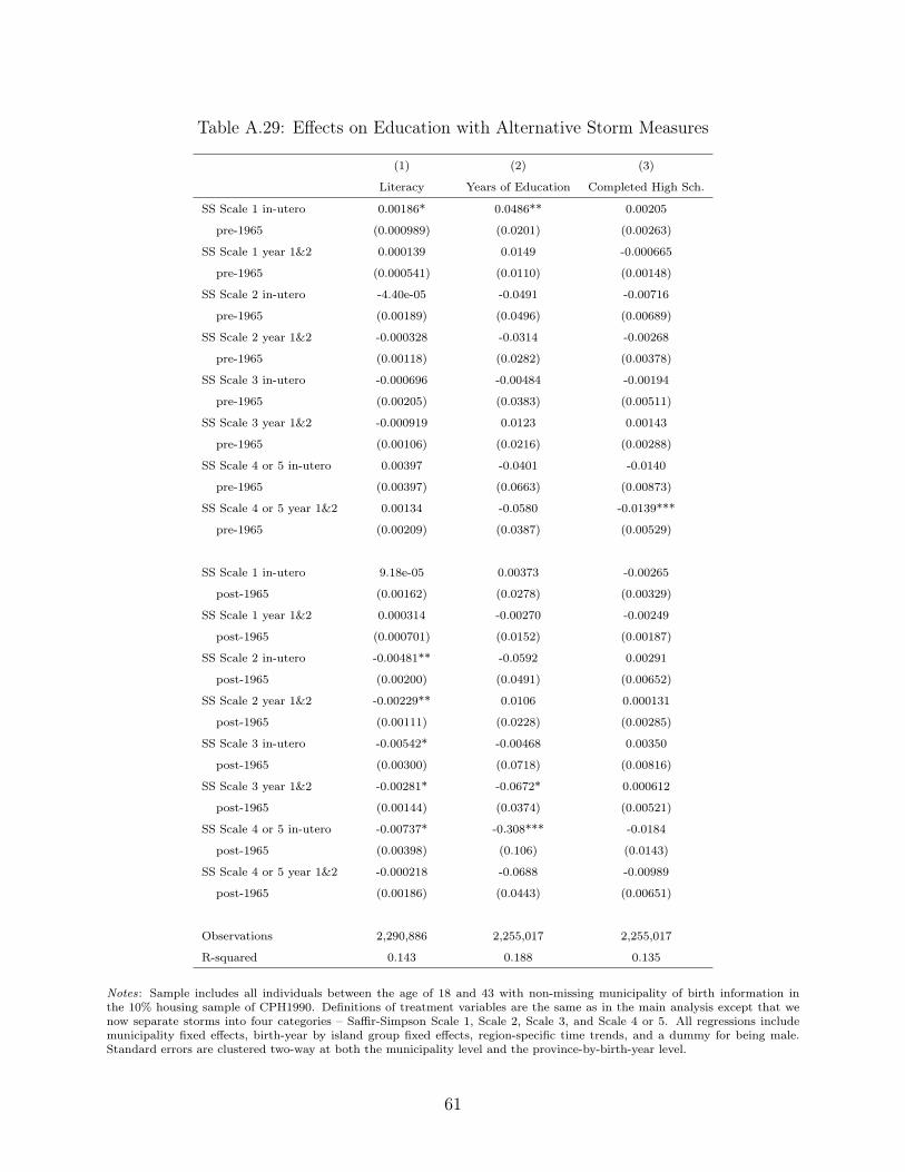
Table A.29: Effects on Education with Alternative Storm Measures

(1) (2) (3)

Literacy Years of Education Completed High Sch.

SS Scale 1 in-utero 0.00186* 0.0486** 0.00205

pre-1965 (0.000989) (0.0201) (0.00263)

SS Scale 1 year 1&2 0.000139 0.0149 -0.000665

pre-1965 (0.000541) (0.0110) (0.00148)

SS Scale 2 in-utero -4.40e-05 -0.0491 -0.00716

pre-1965 (0.00189) (0.0496) (0.00689)

SS Scale 2 year 1&2 -0.000328 -0.0314 -0.00268

pre-1965 (0.00118) (0.0282) (0.00378)

SS Scale 3 in-utero -0.000696 -0.00484 -0.00194

pre-1965 (0.00205) (0.0383) (0.00511)

SS Scale 3 year 1&2 -0.000919 0.0123 0.00143

pre-1965 (0.00106) (0.0216) (0.00288)

SS Scale 4 or 5 in-utero 0.00397 -0.0401 -0.0140

pre-1965 (0.00397) (0.0663) (0.00873)

SS Scale 4 or 5 year 1&2 0.00134 -0.0580 -0.0139***

pre-1965 (0.00209) (0.0387) (0.00529)

SS Scale 1 in-utero 9.18e-05 0.00373 -0.00265

post-1965 (0.00162) (0.0278) (0.00329)

SS Scale 1 year 1&2 0.000314 -0.00270 -0.00249

post-1965 (0.000701) (0.0152) (0.00187)

SS Scale 2 in-utero -0.00481** -0.0592 0.00291

post-1965 (0.00200) (0.0491) (0.00652)

SS Scale 2 year 1&2 -0.00229** 0.0106 0.000131

post-1965 (0.00111) (0.0228) (0.00285)

SS Scale 3 in-utero -0.00542* -0.00468 0.00350

post-1965 (0.00300) (0.0718) (0.00816)

SS Scale 3 year 1&2 -0.00281* -0.0672* 0.000612

post-1965 (0.00144) (0.0374) (0.00521)

SS Scale 4 or 5 in-utero -0.00737* -0.308*** -0.0184

post-1965 (0.00398) (0.106) (0.0143)

SS Scale 4 or 5 year 1&2 -0.000218 -0.0688 -0.00989

post-1965 (0.00186) (0.0443) (0.00651)

Observations 2,290,886 2,255,017 2,255,017

R-squared 0.143 0.188 0.135

Notes: Sample includes all individuals between the age of 18 and 43 with non-missing municipality of birth information inthe 10% housing sample of CPH1990. Definitions of treatment variables are the same as in the main analysis except that wenow separate storms into four categories – Saffir-Simpson Scale 1, Scale 2, Scale 3, and Scale 4 or 5. All regressions includemunicipality fixed effects, birth-year by island group fixed effects, region-specific time trends, and a dummy for being male.Standard errors are clustered two-way at both the municipality level and the province-by-birth-year level.

61

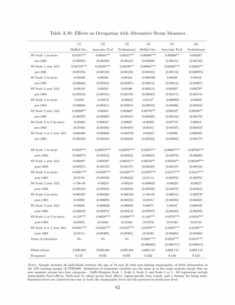
Table A.30: Effects on Occupation with Alternative Storm Measures

(1) (2) (3) (4) (5) (6)

Skilled Occ. Associate Prof. Professional Skilled Occ. Associate Prof. Professional

SS Scale 1 in-utero 0.0105*** 0.00401** 0.00317** 0.00866*** 0.00306** 0.00226*

pre-1965 (0.00335) (0.00168) (0.00145) (0.00309) (0.00151) (0.00130)

SS Scale 1 year 1&2 0.00724*** 0.00338*** 0.00236** 0.00663*** 0.00303*** 0.00205**

pre-1965 (0.00195) (0.00120) (0.00103) (0.00183) (0.00113) (0.000973)

SS Scale 2 in-utero -0.00246 0.00223 0.00424 -0.000536 0.00320 0.00524

pre-1965 (0.00664) (0.00445) (0.00387) (0.00615) (0.00412) (0.00367)

SS Scale 2 year 1&2 -0.00110 0.00210 0.00196 0.000113 0.00305* 0.00279*

pre-1965 (0.00316) (0.00191) (0.00170) (0.00284) (0.00171) (0.00154)

SS Scale 3 in-utero 0.0109 -0.00154 -0.00223 0.0112* -0.000992 -0.00205

pre-1965 (0.00668) (0.00311) (0.00255) (0.00653) (0.00286) (0.00234)

SS Scale 3 year 1&2 0.00809** 0.00344 0.00368* 0.00770** 0.00310* 0.00338**

pre-1965 (0.00379) (0.00209) (0.00191) (0.00340) (0.00184) (0.00172)

SS Scale 4 or 5 in-utero -0.00402 0.00824* 0.00691 -0.00458 0.00773* 0.00618

pre-1965 (0.0100) (0.00456) (0.00450) (0.0101) (0.00437) (0.00443)

SS Scale 4 or 5 year 1&2 0.000488 0.000868 -0.000733 0.00223 0.00209 0.000505

pre-1965 (0.00534) (0.00216) (0.00224) (0.00534) (0.00203) (0.00177)

SS Scale 1 in-utero 0.0259*** 0.00873*** 0.00703*** 0.0259*** 0.00867*** 0.00706***

post-1965 (0.00877) (0.00312) (0.00234) (0.00823) (0.00272) (0.00200)

SS Scale 1 year 1&2 0.00680* 0.00333* 0.00331** 0.00704** 0.00356** 0.00349***

post-1965 (0.00374) (0.00176) (0.00147) (0.00345) (0.00157) (0.00132)

SS Scale 2 in-utero -0.0391*** -0.0180*** -0.0130*** -0.0370*** -0.0171*** -0.0121***

post-1965 (0.0116) (0.00530) (0.00422) (0.0111) (0.00476) (0.00376)

SS Scale 2 year 1&2 -1.59e-05 -0.00210 -0.00219 -0.000645 -0.00225 -0.00217

post-1965 (0.00549) (0.00284) (0.00232) (0.00536) (0.00273) (0.00224)

SS Scale 3 in-utero 0.000437 0.000288 -0.000180 -2.19e-05 -0.000311 -0.000737

post-1965 (0.0208) (0.00698) (0.00535) (0.0191) (0.00586) (0.00448)

SS Scale 3 year 1&2 0.00603 -0.000626 -0.000681 0.00877 0.00107 0.000849

post-1965 (0.00819) (0.00378) (0.00314) (0.00767) (0.00343) (0.00283)

SS Scale 4 or 5 in-utero -0.152*** -0.0659*** -0.0499*** -0.140*** -0.0578*** -0.0434***

post-1965 (0.0395) (0.0166) (0.0126) (0.0373) (0.0148) (0.0110)

SS Scale 4 or 5 year 1&2 -0.0491*** -0.0243*** -0.0197*** -0.0479*** -0.0233*** -0.0188***

post-1965 (0.0111) (0.00495) (0.00391) (0.0108) (0.00484) (0.00388)

Years of education No No No 0.0381*** 0.0252*** 0.0215***

(0.000665) (0.000711) (0.000615)

Observations 2,093,804 2,093,804 2,093,804 2,069,113 2,069,113 2,069,113

R-squared 0.147 0.045 0.037 0.232 0.146 0.125

Notes: Sample includes all individuals between the age of 18 and 43 with non-missing municipality of birth information inthe 10% housing sample of CPH1990. Definitions of treatment variables are the same as in the main analysis except that wenow separate storms into four categories – Saffir-Simpson Scale 1, Scale 2, Scale 3, and Scale 4 or 5. All regressions includemunicipality fixed effects, birth-year by island group fixed effects, region-specific time trends, and a dummy for being male.Standard errors are clustered two-way at both the municipality level and the province-by-birth-year level.

62

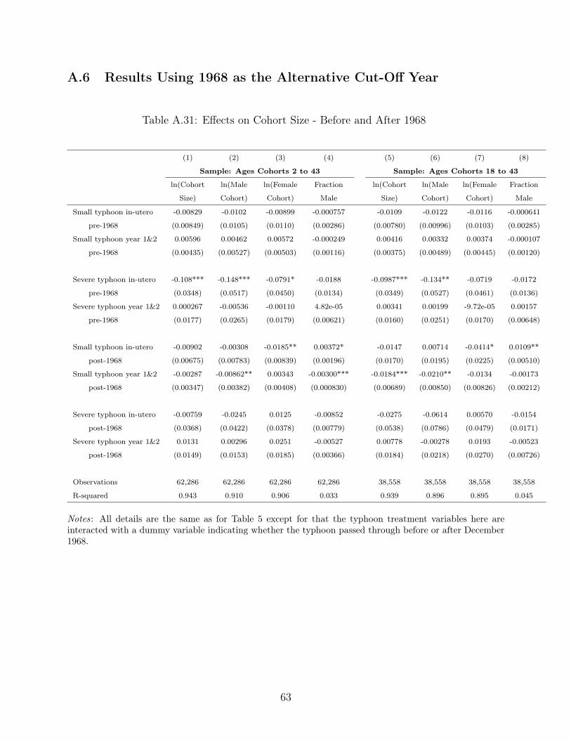
A.6 Results Using 1968 as the Alternative Cut-Off Year

Table A.31: Effects on Cohort Size - Before and After 1968

(1) (2) (3) (4) (5) (6) (7) (8)

Sample: Ages Cohorts 2 to 43 Sample: Ages Cohorts 18 to 43

ln(Cohort ln(Male ln(Female Fraction ln(Cohort ln(Male ln(Female Fraction

Size) Cohort) Cohort) Male Size) Cohort) Cohort) Male

Small typhoon in-utero -0.00829 -0.0102 -0.00899 -0.000757 -0.0109 -0.0122 -0.0116 -0.000641

pre-1968 (0.00849) (0.0105) (0.0110) (0.00286) (0.00780) (0.00996) (0.0103) (0.00285)

Small typhoon year 1&2 0.00596 0.00462 0.00572 -0.000249 0.00416 0.00332 0.00374 -0.000107

pre-1968 (0.00435) (0.00527) (0.00503) (0.00116) (0.00375) (0.00489) (0.00445) (0.00120)

Severe typhoon in-utero -0.108*** -0.148*** -0.0791* -0.0188 -0.0987*** -0.134** -0.0719 -0.0172

pre-1968 (0.0348) (0.0517) (0.0450) (0.0134) (0.0349) (0.0527) (0.0461) (0.0136)

Severe typhoon year 1&2 0.000267 -0.00536 -0.00110 4.82e-05 0.00341 0.00199 -9.72e-05 0.00157

pre-1968 (0.0177) (0.0265) (0.0179) (0.00621) (0.0160) (0.0251) (0.0170) (0.00648)

Small typhoon in-utero -0.00902 -0.00308 -0.0185** 0.00372* -0.0147 0.00714 -0.0414* 0.0109**

post-1968 (0.00675) (0.00783) (0.00839) (0.00196) (0.0170) (0.0195) (0.0225) (0.00510)

Small typhoon year 1&2 -0.00287 -0.00862** 0.00343 -0.00300*** -0.0184*** -0.0210** -0.0134 -0.00173

post-1968 (0.00347) (0.00382) (0.00408) (0.000830) (0.00689) (0.00850) (0.00826) (0.00212)

Severe typhoon in-utero -0.00759 -0.0245 0.0125 -0.00852 -0.0275 -0.0614 0.00570 -0.0154

post-1968 (0.0368) (0.0422) (0.0378) (0.00779) (0.0538) (0.0786) (0.0479) (0.0171)

Severe typhoon year 1&2 0.0131 0.00296 0.0251 -0.00527 0.00778 -0.00278 0.0193 -0.00523

post-1968 (0.0149) (0.0153) (0.0185) (0.00366) (0.0184) (0.0218) (0.0270) (0.00726)

Observations 62,286 62,286 62,286 62,286 38,558 38,558 38,558 38,558

R-squared 0.943 0.910 0.906 0.033 0.939 0.896 0.895 0.045

Notes: All details are the same as for Table 5 except for that the typhoon treatment variables here areinteracted with a dummy variable indicating whether the typhoon passed through before or after December1968.

63

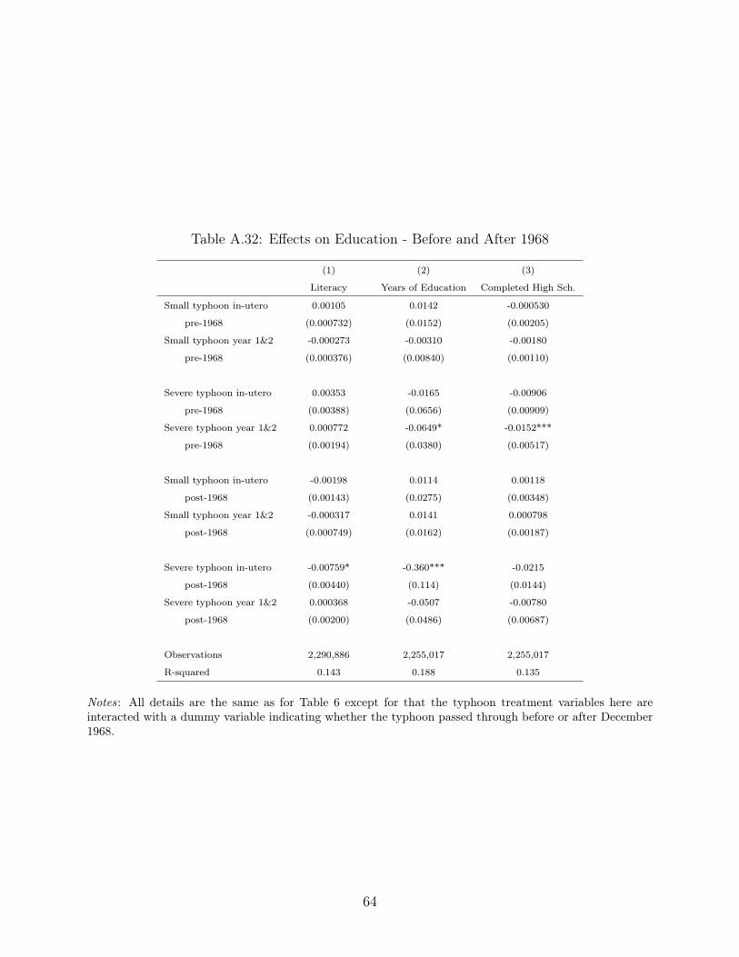
Table A.32: Effects on Education - Before and After 1968

(1) (2) (3)

Literacy Years of Education Completed High Sch.

Small typhoon in-utero 0.00105 0.0142 -0.000530

pre-1968 (0.000732) (0.0152) (0.00205)

Small typhoon year 1&2 -0.000273 -0.00310 -0.00180

pre-1968 (0.000376) (0.00840) (0.00110)

Severe typhoon in-utero 0.00353 -0.0165 -0.00906

pre-1968 (0.00388) (0.0656) (0.00909)

Severe typhoon year 1&2 0.000772 -0.0649* -0.0152***

pre-1968 (0.00194) (0.0380) (0.00517)

Small typhoon in-utero -0.00198 0.0114 0.00118

post-1968 (0.00143) (0.0275) (0.00348)

Small typhoon year 1&2 -0.000317 0.0141 0.000798

post-1968 (0.000749) (0.0162) (0.00187)

Severe typhoon in-utero -0.00759* -0.360*** -0.0215

post-1968 (0.00440) (0.114) (0.0144)

Severe typhoon year 1&2 0.000368 -0.0507 -0.00780

post-1968 (0.00200) (0.0486) (0.00687)

Observations 2,290,886 2,255,017 2,255,017

R-squared 0.143 0.188 0.135

Notes: All details are the same as for Table 6 except for that the typhoon treatment variables here areinteracted with a dummy variable indicating whether the typhoon passed through before or after December1968.

64

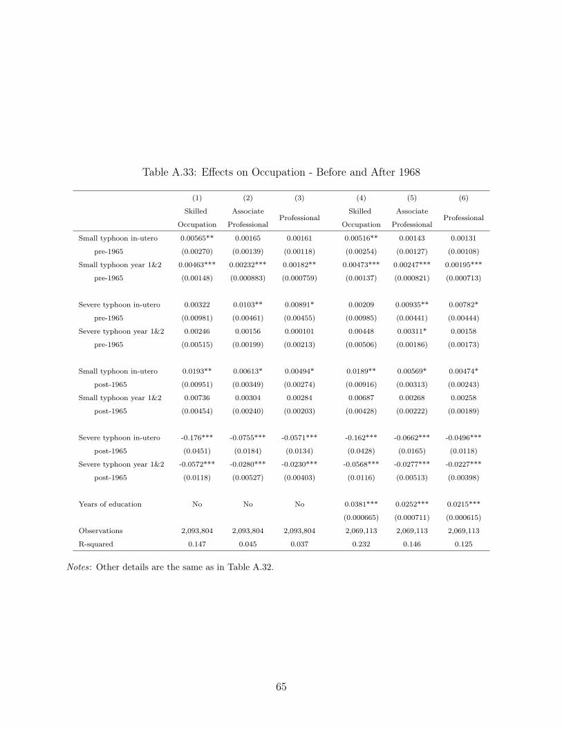
Table A.33: Effects on Occupation - Before and After 1968

(1) (2) (3) (4) (5) (6)

Skilled AssociateProfessional

Skilled AssociateProfessional

Occupation Professional Occupation Professional

Small typhoon in-utero 0.00565** 0.00165 0.00161 0.00516** 0.00143 0.00131

pre-1965 (0.00270) (0.00139) (0.00118) (0.00254) (0.00127) (0.00108)

Small typhoon year 1&2 0.00463*** 0.00232*** 0.00182** 0.00473*** 0.00247*** 0.00195***

pre-1965 (0.00148) (0.000883) (0.000759) (0.00137) (0.000821) (0.000713)

Severe typhoon in-utero 0.00322 0.0103** 0.00891* 0.00209 0.00935** 0.00782*

pre-1965 (0.00981) (0.00461) (0.00455) (0.00985) (0.00441) (0.00444)

Severe typhoon year 1&2 0.00246 0.00156 0.000101 0.00448 0.00311* 0.00158

pre-1965 (0.00515) (0.00199) (0.00213) (0.00506) (0.00186) (0.00173)

Small typhoon in-utero 0.0193** 0.00613* 0.00494* 0.0189** 0.00569* 0.00474*

post-1965 (0.00951) (0.00349) (0.00274) (0.00916) (0.00313) (0.00243)

Small typhoon year 1&2 0.00736 0.00304 0.00284 0.00687 0.00268 0.00258

post-1965 (0.00454) (0.00240) (0.00203) (0.00428) (0.00222) (0.00189)

Severe typhoon in-utero -0.176*** -0.0755*** -0.0571*** -0.162*** -0.0662*** -0.0496***

post-1965 (0.0451) (0.0184) (0.0134) (0.0428) (0.0165) (0.0118)

Severe typhoon year 1&2 -0.0572*** -0.0280*** -0.0230*** -0.0568*** -0.0277*** -0.0227***

post-1965 (0.0118) (0.00527) (0.00403) (0.0116) (0.00513) (0.00398)

Years of education No No No 0.0381*** 0.0252*** 0.0215***

(0.000665) (0.000711) (0.000615)

Observations 2,093,804 2,093,804 2,093,804 2,069,113 2,069,113 2,069,113

R-squared 0.147 0.045 0.037 0.232 0.146 0.125

Notes: Other details are the same as in Table A.32.

65

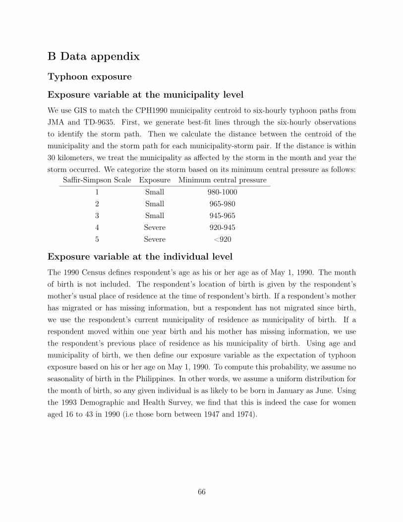
B Data appendix

Typhoon exposure

Exposure variable at the municipality level

We use GIS to match the CPH1990 municipality centroid to six-hourly typhoon paths fromJMA and TD-9635. First, we generate best-fit lines through the six-hourly observationsto identify the storm path. Then we calculate the distance between the centroid of themunicipality and the storm path for each municipality-storm pair. If the distance is within30 kilometers, we treat the municipality as affected by the storm in the month and year thestorm occurred. We categorize the storm based on its minimum central pressure as follows:

Saffir-Simpson Scale Exposure Minimum central pressure1 Small 980-10002 Small 965-9803 Small 945-9654 Severe 920-9455 Severe <920

Exposure variable at the individual level

The 1990 Census defines respondent’s age as his or her age as of May 1, 1990. The monthof birth is not included. The respondent’s location of birth is given by the respondent’smother’s usual place of residence at the time of respondent’s birth. If a respondent’s motherhas migrated or has missing information, but a respondent has not migrated since birth,we use the respondent’s current municipality of residence as municipality of birth. If arespondent moved within one year birth and his mother has missing information, we usethe respondent’s previous place of residence as his municipality of birth. Using age andmunicipality of birth, we then define our exposure variable as the expectation of typhoonexposure based on his or her age on May 1, 1990. To compute this probability, we assume noseasonality of birth in the Philippines. In other words, we assume a uniform distribution forthe month of birth, so any given individual is as likely to be born in January as June. Usingthe 1993 Demographic and Health Survey, we find that this is indeed the case for womenaged 16 to 43 in 1990 (i.e those born between 1947 and 1974).

66

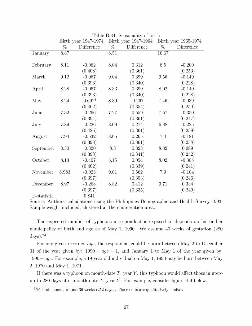
Table B.34: Seasonality of birthBirth year 1947-1974 Birth year 1947-1964 Birth year 1965-1974

% Difference % Difference % DifferenceJanuary 8.87 8.51 10.67

February 8.11 -0.062 8.04 0.312 8.5 -0.200(0.408) (0.361) (0.253)

March 9.12 -0.067 9.04 0.399 9.56 -0.149(0.393) (0.340) (0.228)

April 8.28 -0.067 8.33 0.399 8.02 -0.149(0.393) (0.340) (0.228)

May 8.24 -0.692* 8.39 -0.267 7.46 -0.039(0.402) (0.354) (0.250)

June 7.32 -0.266 7.27 0.559 7.57 -0.350(0.394) (0.361) (0.247)

July 7.89 -0.226 8.09 0.274 6.88 -0.225(0.425) (0.361) (0.239)

August 7.94 -0.532 8.05 0.265 7.4 -0.181(0.398) (0.361) (0.258)

September 8.30 -0.320 8.3 0.328 8.32 0.089(0.398) (0.341) (0.252)

October 8.13 -0.407 8.15 0.054 8.02 -0.308(0.402) (0.339) (0.241)

November 8.983 -0.023 9.01 0.562 7.9 -0.104(0.397) (0.353) (0.246)

December 8.97 -0.268 8.82 0.412 9.71 0.334(0.397) (0.335) (0.240)

F-statistic 0.841Source: Authors’ calculations using the Philippines Demographic and Health Survey 1993.Sample weight included, clustered at the enumeration area.

The expected number of typhoons a respondent is exposed to depends on his or hermunicipality of birth and age as of May 1, 1990. We assume 40 weeks of gestation (280days).23

For any given recorded age, the respondent could be born between May 2 to December31 of the year given by: 1990 � age � 1, and January 1 to May 1 of the year given by:1990�age. For example, a 19-year old individual on May 1, 1990 may be born between May2, 1970 and May 1, 1971.

If there was a typhoon on month-date T , year Y , this typhoon would affect those in uteroup to 280 days after month-date T , year Y . For example, consider figure B.4 below.

23For robustness, we use 36 weeks (252 days). The results are qualitatively similar.

67

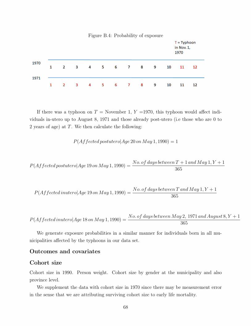
Figure B.4: Probability of exposure

If there was a typhoon on T = November 1, Y =1970, this typhoon would affect indi-viduals in-utero up to August 8, 1971 and those already post-utero (i.e those who are 0 to2 years of age) at T . We then calculate the following:

P (Affected postutero|Age 20 onMay 1, 1990) = 1

P (Affected postutero|Age 19 onMay 1, 1990) =No. of days between T + 1 andMay 1, Y + 1

365

P (Affected inutero|Age 19 onMay 1, 1990) =No. of days between T andMay 1, Y + 1

365

P (Affected inutero|Age 18 onMay 1, 1990) =No. of days betweenMay 2, 1971 andAugust 8, Y + 1

365

We generate exposure probabilities in a similar manner for individuals born in all mu-nicipalities affected by the typhoons in our data set.

Outcomes and covariates

Cohort size

Cohort size in 1990. Person weight. Cohort size by gender at the nunicipality and alsoprovince level.

We supplement the data with cohort size in 1970 since there may be measurement errorin the sense that we are attributing surviving cohort size to early life mortality.

68

Exposure in CPH 1970 is at the province level. We define it similarly-instead of exposedmunicipality, we change it to province. This is a noisy measure, but this is the best we haveto address the concerns on later life mortality in CPH 1990.

Education

The 1990 Census categorizes education into elementary 1 to 6, high school 1 to 4. Themajority of students begin formal schooling at 6, so respondents should be aged 16 when theycomplete high school (with no grade repetition). Beyond 10 years of education (high schoolcompletion), we use the Census categories for post-secondary education, which includesbachelor’s degrees, one to three year diploma programs, and post graduate education.

Occupational skill level

We categorize occupation into professional, semi-professional, and skilled occupation basedon the the 1990 Census categories. CPH1990 categorizes occupation into 4-digit categories.The first question in the Census captures occupation in the past year, while the secondcaptures occupation in the past week. We use 2-digit occupation codes in the past year, andin cases where this variable is not reported, we use occupation in the past week. We excludenon-gainful occupation, which includes volunteers, housekeepers, students, pensioners andother retirees, disabled, and other non-gainful or no reported activity.

We generate an indicator for professional if respondents report: manager or professional.An indicator for semi-professional equals one if the respondent reports: manager, profes-sional, or technician. We then create an indicator for skilled occupation based on the secondISCO (International Standard Classification of Occupations) skilled level or higher. ISCOis part of the international family of economic and social classifications of the InternationalLabour Organization. For example, in agriculture, CPH1990 separates ’skilled rice farmworker’ from ’farm laborer’, and we code the two occupations under different skill levels.

C A Conceptual Framework for Culling and Scarring

We present a modified version of the “fetal origins” model in Almond (2006) to illustratehow in-utero exposure to typhoons and changes in post-disaster relief policies could interactto create the culling and scarring effects we have documented in this paper.

Following Almond (2006), we allow a severe typhoon to have two potential effects on fetalhealth: (1) a negative shift in the unobserved distribution of fetal health (scarring) and (2) areduction in the survival odds conditional on health. Both effects contribute to culling. Thelatter may happen as a result of deteriorating medical care and a shortage of clean waterand food in the ensuing weeks after a severe typhoon. The fetal origins hypothesis asserts

69

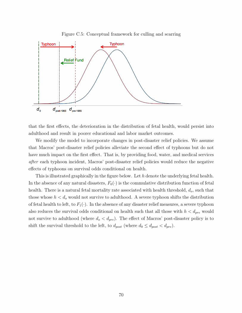
Figure C.5: Conceptual framework for culling and scarring

that the first effects, the deterioration in the distribution of fetal health, would persist intoadulthood and result in poorer educational and labor market outcomes.

We modify the model to incorporate changes in post-disaster relief policies. We assumethat Macros’ post-disaster relief policies alleviate the second effect of typhoons but do nothave much impact on the first effect. That is, by providing food, water, and medical servicesafter each typhoon incident, Macros’ post-disaster relief policies would reduce the negativeeffects of typhoons on survival odds conditional on health.

This is illustrated graphically in the figure below. Let h denote the underlying fetal health.In the absence of any natural disasters, F0(·) is the commulative distribution function of fetalhealth. There is a natural fetal mortality rate associated with health threshold, d

o

, such thatthose whose h < d

o

would not survive to adulthood. A severe typhoon shifts the distributionof fetal health to left, to F1(·). In the absence of any disaster relief measures, a severe typhoonalso reduces the survival odds conditional on health such that all those with h < d

pre

wouldnot survive to adulthood (where d

o

< d

pre

). The effect of Macros’ post-disaster policy is toshift the survival threshold to the left, to d

post

(where d0 d

post

< d

pre

).

70