Embed Size (px)
Citation preview
Working Paper 356February 2014
Scarcity without Leviathan: The Violent Effects of Cocaine Supply Shortages in the Mexican Drug War
Abstract
Using the case of the cocaine trade in Mexico as a relevant and salient example, this paper shows that scarcity leads to violence in markets without third party enforcement. We construct a model in which supply shortages increase total revenue when demand is inelastic. If property rights over revenues are not well defined because of the lack of reliable third party enforcement, the incentives to prey on others and avoid predation by exercising violence increase with scarcity, thus increasing violence. We test our model and the proposed channel using data for the cocaine trade in Mexico. We found that exogenous supply shocks originated in changes in the amount of cocaine seized in Colombia (Mexico's main cocaine supplier) create scarcity and increase drug-related violence in Mexico.
In accordance with our model, the effect of cocaine scarcity on violence is larger near US entry points; in locations contested by several cartels; and where, due to high support for the PAN party, crackdowns on the cocaine trade have been more frequent. Our estimates suggest that, for the period 2006-2010, scarcity created by more efficient interdiction policies in Colombia may account for 21.2% and 46% of the increase in homicides and drug-related homicides, respectively, experienced in the north of the country. At least in the short run, scarcity created by Colombian supply reduction efforts has had negative spillovers in the form of more violence in Mexico under the so-called War on Drugs.
JEL Codes: D74, K42
Keywords: Rule of Law, War on Drugs, Violence, Illegal Markets, Mexico.
www.cgdev.org
Juan Camilo Castillo, Daniel Mejía, and Pascual Restrepo
Scarcity without Leviathan: The Violent Effects of Cocaine Supply Shortages in the Mexican Drug War
Juan Camilo CastilloUniversidad de los Andes
Daniel MejiaUniversidad de los Andes
Pascual RestrepoMassachusetts Institute of Technology
We are grateful to Daron Acemoglu, Dora Costa, Leopoldo Fergusson, Claudio Ferraz, and Dorothy Kronick, as well as seminar participants at Universidad de los Andes, Stanford, UCLA, and LACEA for their very helpful comments and suggestions. Melissa Dell, Horacio Larreguy, and Viridiana Ríos kindly provided the data we use in this paper. We gratefully acknowledge funding from the Open Society Foundations and from the Center for Global Development. All remaining errors are ours. E-mails: [email protected], [email protected], [email protected].
CGD is grateful for contributions from its funders and board of directors in support of this work.
Juan Camilo Castillo, Daniel Mejia, and Pascual Restrepo. 2014. "Scarcity without Leviathan: The Violent Effects of Cocaine Supply Shortages in the Mexican Drug War." CGD Working Paper 356. Washington, DC: Center for Global Development.
http://www.cgdev.org/publication/scarcity-without-leviathan-violent-effects-cocaine-supply-shortages-mexican-drug-war
Center for Global Development2055 L Street NW
Washington, DC 20036
202.416.4000(f ) 202.416.4050
www.cgdev.org
The Center for Global Development is an independent, nonprofit policy research organization dedicated to reducing global poverty and inequality and to making globalization work for the poor. Use and dissemination of this Working Paper is encouraged; however, reproduced copies may not be used for commercial purposes. Further usage is permitted under the terms of the Creative Commons License.
The views expressed in CGD Working Papers are those of the authors and should not be attributed to the board of directors or funders of the Center for Global Development.
Foreword by Michael Clemens
The 2,000 mile border between the US and Mexico is an economic cliff, the largest GDP per capita differential at any land border on earth. Across this fault-line, the two nations continue a deep and centuries-old exchange of goods, services, investment, labor, culture, and ideas.
Some of those interactions happen through flourishing, transnational illicit markets—such as for drugs, arms, and labor—with major economic and social effects for both sides. The political economy of these markets is complex and poorly understood. It is shaped by a policy approach that is today dominated by unilateral, domestic law enforcement.
This paper was commissioned by CGD’s Beyond the Fence study group. Castillo, Mejía and Restrepo provide a rigorous new evidence of the ripple effects of enforcement policy via transnational illicit markets. First, they measure for the first time how antinarcotics interdiction in Colombia affects cocaine prices far away—in Mexico. Second, they show how the resulting change in cocaine prices leads to violence in Mexico, above and beyond violence caused by local enforcement efforts. This transnational mechanism can explain roughly one fifth of the stunning rise in murders in Mexico after 2006.
CGD created Beyond the Fence in 2013 to generate rigorous new research on how policy decisions on one side of the border ripple to the other side through illicit markets, and to inform a policy debate on more bilateral approaches to innovative regulation. The group brings together some of the world’s leading social scientists and policy innovators. The dual meaning of the name represents a desire for researchers to investigate the effects of policy that cross the fence, and for policymakers to reach beyond unilateral enforcement approaches.
“Hereby it is manifest that during the time men live without a common power to
keep them all in awe, they are in that condition which is called war; and such a war
as is of every man against every man. [ . . . ] In such condition there is no place for
industry [. . . ] ; no account of time; no arts; no letters; no society; and which is worst
of all, continual fear, and danger of violent death; and the life of man, solitary, poor,
nasty, brutish, and short.”
Thomas Hobbes, 1651
Leviathan
Book I, chapter XIII
1 Introduction
According to Thomas Hobbes, in a world without the rule of law, in which the state
does not have the monopoly of violence and where no reliable third party can enforce
laws and contracts, the life of man becomes “nasty, brutish and short” (Hobbes, 1651).
The rule of law and monopoly of violence by a central authority—the Leviathan—are
essential requirements for the absence of conflict and violence. Contemporary writers
like Steven Pinker have also argued that the rise of the Leviathan was one of the main
driving forces behind the decline in violence that has been observed during the last
millennium (see Pinker, 2011). The logic behind this observation is simple: Outside
the rule of law there is no reliable third party enforcement and property rights are
poorly defined; wealth and assets can be appropriated by others through the use of
force, and violence becomes the only rational choice. Not only does the exercise of
violence allow people to prey on others; it also protects them from potential predators.
In such an environment appropriation and protection become what Hirshleifer (2001)
has termed “the dark side of the force”.
Despite the great expansion of the state and its monopoly of violence since Hobbes’
time, there are still many regions, markets, and moments, both past and present, that
lie outside the scope of the Leviathan, and in which violent appropriation and private
protection are the rule rather than the exception. In many developing countries there
are large areas with no state presence, where the monopoly of violence is disputed
among local strongmen (see Acemoglu et al., 2013; Fearon and Laitin, 2003; Sanchez
de la Sierra, 2014). This creates large conflicts between warlords over the extraction
and control of valuable resources and their rents (see Skaperdas, 2002). Markets for
illegal goods are another important example, where illegality precludes the possibility
1
of using the state as a source of third-party enforcement. Contemporaneous illegal drug
markets in Colombia, Mexico, and Afghanistan are all ruled by illegal armed groups
that frequently resort to violence in order to solve disputes and protect (de facto)
property rights. The scale and salience of violence may vary, but other markets with
poorly defined property rights are constantly subject to violence as well, independently
of the type of goods transacted. For instance, a recent piece in The New York Times
describes the use of violence by fisherman involved in the banned sea cucumber trade
in Mexico1.
But examples are not limited to developing nations. In Sicily, the violent mafia
started as a dual organization that specialized both in extortion and offering protection
for the explotation of sulfur mines (see Buonanno et al., 2012). The mafia’s business
model was only profitable because of the weak law enforcement institutions in the Italian
South. Later, the mafia diversified and started selling protection in other trades. There
was demand for private protection only because the Leviathan was absent in such
environments (see Gambetta, 1996). During the settlement of the American West,
Scots-Irish herders developed a “culture of honor”, in which people were expected to
respond with violence against any threat (see Nisbett and Cohen, 1996; Grosjean, 2013).
These cultural norms are a violent substitute for a third party that settles disputes
among herders and punishes those attempting to steal herds.
In this paper we analyze the role of scarcity in environments that lack reliable third
party enforcement. By third party enforcement we mean that market participants
are subject to the state’s monopoly of violence—the rule of law, which is used to
enforce property rights and enforce contracts in an impartial and reliable way. As our
discussion above underscores, the intensity and salience of violence varies from example
to example. Thus, it becomes important to understand its determinants. We study
the role of scarcity—or supply shortages—as one important factor that can potentially
exacerbate the use of violence in market environments without third party enforcement.
Our basic intuition is that scarcity increases violence if the demand for certain goods
whose market is illegal is inelastic. In this case, a decrease in supply causes a larger
increase in prices, therefore increasing total revenues and the stakes. This leads to more
predation and violence.
We study this question in the context of Mexico and the cocaine trade. Mexico
has witnessed a dramatic increase in violence: The homicide rate in 2010 was almost
1Because sea cucumbers are extracted from the bottom of the ocean, they do not haveproperly defined property rights, and this has caused fights among neighboring fisherman com-munities. See the full story here: http://www.nytimes.com/2013/03/20/world/americas/
quest-for-illegal-gain-at-the-sea-bottom-divides-fishing-communities.html?_r=0.
2
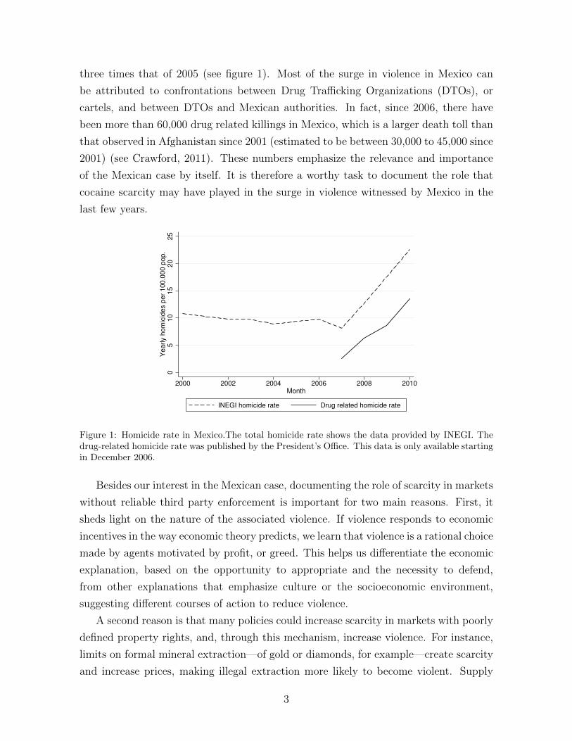
three times that of 2005 (see figure 1). Most of the surge in violence in Mexico can
be attributed to confrontations between Drug Trafficking Organizations (DTOs), or
cartels, and between DTOs and Mexican authorities. In fact, since 2006, there have
been more than 60,000 drug related killings in Mexico, which is a larger death toll than
that observed in Afghanistan since 2001 (estimated to be between 30,000 to 45,000 since
2001) (see Crawford, 2011). These numbers emphasize the relevance and importance
of the Mexican case by itself. It is therefore a worthy task to document the role that
cocaine scarcity may have played in the surge in violence witnessed by Mexico in the
last few years.
05
10
15
20
25
Yearly h
om
icid
es p
er
100.0
00 p
op.
2000 2002 2004 2006 2008 2010Month
INEGI homicide rate Drug related homicide rate
Figure 1: Homicide rate in Mexico.The total homicide rate shows the data provided by INEGI. Thedrug-related homicide rate was published by the President’s Office. This data is only available startingin December 2006.
Besides our interest in the Mexican case, documenting the role of scarcity in markets
without reliable third party enforcement is important for two main reasons. First, it
sheds light on the nature of the associated violence. If violence responds to economic
incentives in the way economic theory predicts, we learn that violence is a rational choice
made by agents motivated by profit, or greed. This helps us differentiate the economic
explanation, based on the opportunity to appropriate and the necessity to defend,
from other explanations that emphasize culture or the socioeconomic environment,
suggesting different courses of action to reduce violence.
A second reason is that many policies could increase scarcity in markets with poorly
defined property rights, and, through this mechanism, increase violence. For instance,
limits on formal mineral extraction—of gold or diamonds, for example—create scarcity
and increase prices, making illegal extraction more likely to become violent. Supply
3
reduction policies in drug markets create scarcity and may end up inducing more vio-
lence. Commercial restrictions to trade in some resource-abundant countries with poor
institutions could increase rents and violence. Moreover, violence would persist in these
environments as long as unprotected revenues are high, so that the stakes remain at-
tractive and the use of violence becomes a profitable strategy. The fact that scarcity
increases violence by raising revenues suggests that policies that reduce revenue and
limit the incentives to prey become the best alternative to actually enforcing property
rights adequately. Thus, recognizing the nature of violence in markets without third
party enforcement and the effect of market forces on its extent, would enable policy
makers to design better policies to prevent it or cope with it.
We construct a simple model that provides insights that apply generally, although
it is motivated by the recent Mexican case. In our model, exogenous (negative) supply
shocks in cocaine markets cause increases in wholesale prices that are larger than the
fall in quantities. Thus, the total revenue from cocaine trafficking activities increases,
and the higher stakes spur more violence. An important assumption for this to hold is
that demand for cocaine is inelastic, as has been documented by various sources such
as Becker et al. (2006)2. The reasoning behind the assumption is that, since cocaine
is an addictive substance, consumers must buy their personal dose regardless of price,
implying an inelastic demand.
In our model, drug cartels fight each other and use violence to be able to extract
more of the higher rents. The use of violence increases when the stakes are higher.
For example, when revenue from the cocaine trade increases, toll collector cartels can
extract greater rents, and thus become more willing to use violence to control a given
territory suitable for the drug trade. In turn, other cartels will also be more likely
to use violence in response, in order to avoid being extorted or preyed upon. When
there are more cocaine rents in the system, there is more cash and assets that can be
appropriated by other cartels, or even by the very members of the same cartel (if it is
not fully cohesive). Rapacity and violence emerge as a consequence. Unlike participants
in well functioning legal markets, cartels do not have reliable third party enforcement
to protect their property and revenue streams from others, or to protect them from
extortion. Violence does not only become an opportunistic strategy to prey on others;
it also becomes a necessity to protect one’s own position and the control of the trade.
Our model shows that the effect of cocaine shortages on violence is larger in places with
more competing organizations (i.e., rival cartels), in places where there is more turnover
and hence informal cooperation arrangements cannot sustain less violent outcomes (i.e.,
2We further discuss the validity of this assumption when we present the model.
4
due to higher arrest rates of cartel leaders), and in places where drug trafficking is more
intense (e.g., the north of Mexico).
We test our model using monthly data from Mexican municipalities from December
2006 to 2010, a period that coincides with what has been called the “Mexican Drug
War”. The Mexican cocaine trade fits perfectly our purposes for several reasons. First,
because cocaine production takes place in the Andes, and most notably in Colombia
during our period of study, we can use changes in interdiction policies in Colombia as
exogenous sources of variation in the supply of cocaine. Second, cocaine demand has
been estimated to be inelastic, especially in the short run3. Third, the illegal nature
of this market precludes the existence of any formal source of third party enforcement,
thus forcing market participants to operate outside the scope of the rule of law, and
forcing market participants to enforce property rights and contracts by themselves.
We focus on high frequency monthly variation in the supply of cocaine from Colom-
bia as a source of shocks to scarcity in cocaine markets in Mexico. This variation is
created by month to month changes in seizures in Colombia, which are arguably exoge-
nous to the Mexican environment. We only focus on high frequency relations because
we believe year to year variation is likely to confound trends in Mexican and Colombian
policies that may be spuriously correlated over time (for instance, Calderon’s war on
drugs, and a shift towards more interdiction efforts in Colombia, both of which increased
steadily since 2006). The key identifying assumptions are, first, that the potential re-
lationship between policies in Mexico and Colombia breaks down at higher frequencies
once we control flexibly for long term time trends, and second, that other determinants
of violence in Mexico are not correlated with interdiction efforts in Colombia at higher
frequencies.
We find that violence increases in Mexico during months with supply shortages
caused by seizures in Colombia. Moreover, violence increases especially in the north,
and within the north, specifically in places close to U.S. entry points, as predicted by our
model. Also, violence increases more in northern municipalities that have historically
voted for PAN, President Felipe Calderon’s party (whose term lasted from December
2006 until November 2012). Because these municipalities were more likely to support
federal government efforts against cartels in their area (see Dell, 2012), the turnover of
cartel leaders was higher. Finally, violence increases more in places with cartel presence,
especially in places with two or more cartels or with two or more rival cartels operating
at the time of the supply shock. The fact that the effect of scarcity is mediated by all
these variables does not only further validate our model, but also shows a wide range of
3Once again, see our detailed discussion about the elasticity of demand in section 4.
5
empirical facts consistent with our proposed mechanism through which scarcity breeds
violence.
Our interpretation of the results is that Colombian supply shocks—which became
larger and more frequent since 2006—have created scarcity, raised prices and con-
tributed to the increase in violence in Mexico. Our preferred estimates suggest that
a 10 metric ton (mt) decrease in the Colombian supply in a given month (Colombia
produced around 43.5 mt per month in 2006) increases the overall homicide rate during
that month by 1.2 log points in all Mexico, by 3.5 log points in the 40% municipalities
closest to the U.S., and by 5.1 log points in the 20% municipalities closest to the U.S.
border. Our estimated effects are even larger as one gets closer to U.S. entry points.
More precisely, our estimated impact is about 14 log points larger near the Mexico-U.S.
border.4 Assuming the size of this effect is the same in the long run, we would conclude
that the reduction in the net cocaine supply from Colombia experienced between 2007
and 2010 (from 43.5 mt to 16.6 mt each month) accounts for about 37 log points of
the 174.5 log point increase of the homicide rate in northern Mexico. Our estimates
suggest that, for the period 2006-2010, scarcity created by more efficient interdiction
policies in Colombia may account for 21.2% and 46% of the increase in homicides and
drug related homicides (see section 6 for the calculations involved for these estimates),
respectively, experienced in the north of the country. At least in the short run, scarcity
created by Colombian supply reduction efforts has had negative spillovers in the form
of more violence in Mexico.
Although our evidence comes from a particular context, we believe that the eco-
nomic forces modeled are present in many commodity markets without reliable third
party enforcement, at least in the short run, if demand is inelastic. Our evidence sug-
gests that scarcity can have larger effects in markets with several rival participants
(monopolies could thus reduce rapacity and violence), in places where the trade is par-
ticularly important (i.e., near places that are abundant in resources required for the
production and transportation of the commodity), and in places with large turnover
among market participants, which precludes the formation of informal arrangements to
enforce property rights. Illegal drug markets are special in that they are illegal, and
hence the lack of reliable third party enforcement becomes a more serious issue than
in markets with weak central state presence. Thus, the magnitude of the effects we
analyze might be smaller in other contexts, but we believe that the economic forces
highlighted in this paper would still operate.
This paper is organized as follows. Section 2 outlines the related literature and
4This is the average effect among the 5% municipalities closest to the U.S.
6
explains our contribution to the literature. In section 3 we revisit the Mexican context
and describe its environment. Section 4 presents a simple model to understand the
effects of scarcity on violence in illegal drug markets and derives some testable predic-
tions. Section 5 presents our estimation strategy, data and empirical results. Section 6
concludes.
2 Related literature
Our paper is related to at least three branches of literature. First, it is related to the
broad literature on property rights and violence. The fact that interpersonal violence
emerges when the state lacks the monopoly of violence is a classic theme in the social
sciences at least since Hobbes (1651), and it has been treated more recently by Elias
(2000) and Pinker (2011). The possibility of using force or the threat of force to
appropriate resources, in contrast to ordinary market transactions, has been present
in the economic literature since Grossman (1991) and Hirshleifer (1991, 1994, 2001).
When property rights are weak, or institutions—such as the rule of law—dysfunctional,
conflict over the access and control of valuable resources could end up increasing violence
through rapacity. This is a variant of the resource curse, in which the presence of
valuable commodities ends up increasing violence by intensifying rapacity, i.e., the
temptation to prey on others and the necessity to defend from potential predators.
Skaperdas (2002) argues that when there is no monopoly of violence, warlords com-
pete for turf, which allows them to extract rents from valuable resources. When the
value of these resources increases so does conflict among warlords. In a similar vein,
Gambetta (1996) argues that the combination of valuable resources with poorly defined
property rights can lead to the emergence of mafia-type organizations that offer private
protection from predation by others or from the mafia itself (i.e., extortion). Collier
and Hoeffler (2004) show that resource booms could be used to finance insurgencies, or
could induce a greedy insurgency to start a civil war in order to control the rents from
these resources (see also Grossman, 1999). However, weak property rights or lack of re-
liable third party enforcement are not sufficient for the rapacity channel to be observed.
For instance, resource booms could also increase wages, and hence the opportunity cost
of people to engage in violence, outweighing the effects of rapacity (see Becker, 1968;
Grossman, 1991).
Just as with the ambiguous theoretical predictions, the empirical findings regard-
ing the effect of an increase in resource revenues—caused by either scarcity or demand
increases—is mixed. For instance, Collier and Hoeffler (2004) find that exports of com-
7
modities have a strong positive effect on the risk of conflict. However, Fearon (2005)
shows that this result is fragile, and that only oil production appears to be an impor-
tant determinant of conflict onset after a resource boom. His interpretation is that oil
produces an easy source of financing for rebel groups, rather than oil rents being con-
tested by armed groups. On the other hand, using a panel of African countries, Miguel
et al. (1994) show that higher national income, instrumented using rainfall, reduces
the likelihood of conflict, probably because the opportunity cost channel dominates in
this case. Bruckner and Ciccone (2010) reach a similar conclusion using variation in
commodity prices. Dube and Vargas (2013) find that coffee booms– which are likely to
increase wages–reduce violence in Colombia, while oil booms– which are not likely to
increase wages– increase violence.
A paper that is very closely related to ours is Buonanno et al. (2012). They find that
mafia-type organizations were more likely to appear in Sicilian municipalities with sulfur
extraction, a valuable commodity with poorly defined property rights. The timing of
the emergence of these organizations coincided with a large boom in sulfur prices. On a
similar vein, Couttenier et al. (2013) show that, during the U.S. gold rush, interpersonal
violence increased near mineral discoveries, but only when there was no state presence
at the time of the discovery. They refer to this violence as a variant of the resource
curse. Both papers support the view advanced here that scarcity—understood as low
demand relative to supply that triggers an increase in prices and revenues—increases
violence in commodity markets with poorly defined property rights through a rapacity
channel. A full review of this literature is beyond the scope of our paper, but the
interested reader is referred to Ross (2004).5
We contribute to this literature by studying the role of rapacity in the context of
an illegal commodity. Illegal commodities are, in our view, one natural example in
which rapacity—or the willingness to appropriate—should be strong, given that their
illegal character precludes market participants from the possibility of relying on a third
party to enforce property rights and fulfill contracts. When property rights are not
centrally enforced, the temptation to prey and the need to protect from others make
violence a natural outcome. Consistent with this view, we show that scarcity has an
5Another branch of literature does not focus on the role of commodities but on the emergence ofviolence when property rights are weak. Grosjean (2013) studies the emergence of the culture of honorin the U.S. South, and finds that places with more herding during the settlement period were, and stillremain, more violent. Moreover, this only occurs in the Deep South, where institutions were weak andproperty rights over herds were poorly enforced by a central authority, suggesting that the rapacitychannel might have been in place. She interprets these findings as supporting Nisbett and Cohen’shypothesis that the lack of property rights over herds led to the use of inter-personal violence as acostly substitute.
8
effect on violence through the rapacity channel by increasing total revenue if demand is
inelastic. The fact that violence increases differentially in areas that are more important
for cocaine trafficking, when there are more cartels contesting these areas, or when
there is large turnover further suggest that the specific channel through which scarcity
increases violence is rapacity. We cannot rule out the presence of the opportunity cost
channel, but it appears to be dominated in this particular market, which is the case
as long as the labor share of the Mexican cocaine trade is small relative to the whole
economy (see Dal Bo and Dal Bo, 2011).6
Our paper is also related to literature on violence in illegal markets, and more
particularly to violence in drug markets. This literature started with the classification
of drug related violence by Goldstein (1985), according to which drug markets can
breed violence through three different channels: First, through pharmacological violence
consuming drugs may lead users to a mental state in which they are more prone to
aggressive behaviors and violence; second, through economic compulsive violence drug
consumers may engage in property crime in order to be able to sustain their costly
habit. These two channels are unrelated to the supply side of drug markets that we
study in this paper. The third channel is systemic violence among suppliers, and is
caused by the fact that illegal markets lack reliable third party enforcement, and their
participants are pushed outside of the scope of the rule of law. Thus, systemic violence
is exactly the type of violence we have discussed so far, which occurs when property
rights are poorly defined and the temptation to appropriate others’ resources arises.
Several papers have studied the correlation between violence and the supply side
of drug markets with some mixed findings. We will only focus on those which, in our
view, have taken seriously the endogeneity issues that arise when trying to estimate the
causal effect of illegal drug markets on systemic violence. Angrist and Kugler (2008)
exploit a large upsurge in coca cultivation in Colombia caused by an exogenous change
in Peruvian policy that deterred cocaine cultivation in Peru during the first half of
the 1990s. As a consequence, violence increased in Colombia, especially in states that
already produced coca leaves by 1994. Mejıa and Restrepo (2013) also study the case of
Colombia. They construct an index of suitability for coca cultivation at the municipal
level, and show that its interaction with different demand shocks for Colombian cocaine
predicts within-municipality variation in the extent of coca cultivation. They use this
index as an exogenous source of variation to set up an instrumental variables estimator
6Levitt and Venkatesh (2000) offer some evidence suggesting a small labor share in the drug dealingbusiness. They find that wages for gang members are barely above the minimum wage. Their datacomes from a gang involved in drug dealing in an anonymous American city, so their findings do notnecessarily apply to Mexican cartels.
9
and conclude that increases in coca cultivation cause more violence. The interpretation
of their results relies on the fact that illegal armed groups fight each other (and the
government) over the control of territories suitable for coca cultivation and cocaine
production.
Some other works focus on illegal goods other than drugs. Owens (2011a) finds no
effect of dry laws on homicides and argues that demographics were the main driving
force behind the increase in crime during the alcohol prohibition period. However, in a
subsequent study, Owens (2011b) shows that the Temperance movement did increase
violence among young people, who were more likely to be involved in the supply side
of alcohol distribution than older people. Likewise, Garcıa-Jimeno (2012) shows that
alcohol prohibition, especially the intensity of enforcement, caused an increase in crime
in U.S. cities. The relation between illegal markets and violence, however, is not limited
to addictive goods. Chimeli and Soares (2010) explore how illegality itself generates
violence in a completely different market: mahogany exploitation in the Brazilian Ama-
zon. Mahogany trade in Brazil was initially legal, but it was suddenly prohibited in
a short period of time, between March 1999 and October 2001. The authors use a
difference in difference approach and conclude that violence increased differentially due
to prohibition in places where mahogany extraction was a natural phenomenon.
Our paper contributes to this literature by identifying systemic violence, and char-
acterizing how it changes with scarcity in the context of the Mexican drug war. In
particular, we document how drug related violence in the Mexican cocaine trade be-
haves as predicted in a model in which violence follows a profit maximizing logic. In
particular, violence in Mexico responds to economic incentives and to variations in the
value of the drug trade created by supply shocks in Colombia. This is the defining
characteristic of systemic violence. Thus, although we are not directly estimating the
contribution of drug trafficking to violence, we are showing that to a large extent, the
nature of drug related violence in Mexico is related to profit incentives and rapacity
effects, and not to other social or cultural explanations. Our paper adds to the in-
creasing body of evidence suggesting that participants in illegal drug markets rely on
violence to prey on others and protect themselves because of lack of reliable third party
enforcement. The resulting systemic violence in the supply side of drug markets is, in
our opinion, the largest cost of the war on drugs. Our paper also contributes to this
literature by showing that supply reduction policies may increase violence by increas-
ing total revenue, and create strong spillovers whereby policy changes in one country
affect security in other countries (see Castillo (2013) and Mejıa and Restrepo (2013)
for similar theoretical and empirical results).
10
Finally, our paper is related to an ongoing debate about the causes of the large up-
surge in violence observed in Mexico since 2006. Many observers have pointed fingers at
president Calderon’s strategy as the main reason for the increase in homicides observed
in the last years. More precisely, many observers and security analysts have argued
that Calderon’s strategy of frontally attacking drug cartels, especially targeting their
leaders, has been the main force behind the surge in homicides since 2007. They argue
that Calderon’s strategy of beheading drug cartels, either by killing or capturing their
leaders, has led to internal disputes over the control of this illegal business by competing
cartels or by lower ranked members of the same drug trafficking organizations. Also,
critics argue, the strategy led to the splitting of major cartels into smaller ones7. Some
studies supporting this position are Guerrero (2010, 2011a) and Merino (2011). Some
other studies defend the government’s actions, such as Poire and Martınez (2011), who
argue that the strategy of capturing or killing cartel leaders does not increase violence,
and Villalobos (2012), who supports Calderon’s strategy arguing that in order to elim-
inate drug related violence, a period of higher levels of violence was necessary before
homicide rates start going down.
More recent papers have addressed this question taking endogeneity issues seriously
when trying to estimate the effect of Calderon’s policies against drug cartels on the
levels of violence. Dell (2012) uses a regression discontinuity design, comparing those
municipalities where the PAN, Calderon’s party, won the local elections by a small
margin vis-a-vis those municipalities in which the PAN lost by a small margin, expecting
more violence where the PAN won. The intuition behind her identification strategy is
that it was easier for the Federal Government to intervene in municipalities with a
PAN mayor, thus making Calderon’s war on drugs more intense in these places. The
study concludes that frontal actions against DTOs have caused an important increase
in the levels of violence and created spillovers in neighboring municipalities. On the
other hand, another study by Calderon et al. (2012) combines a difference in differences
methodology with synthetic control groups and shows that Calderon’s intervention did
have an effect on the levels of violence, but it was only a temporal effect (contrary to
what Guerrero (2011a) argues). In a different vein, Dube et al. (2012) shift the focus to
U.S. gun control policies. In particular, they find that violence in Mexico increased as
a consequence of the 2004 expiration of the U.S. Federal Assault Weapons Ban, which
created a positive shock of gun availability in Mexico. In another paper, Dube et al.
(2013) show that negative agricultural shocks contributed to the rise of the Mexican
7Grillo (2011) and Valdes (2013) provide thorough reviews of the history of drug trafficking inMexico and its nexus with crime and violence
11
drug sector. The authors also find that, consistent with our findings, violence increased
as a consequence.
Our paper contributes to this literature by showing that besides U.S. assault guns,
negative agricultural shocks and Calderon’s policies spearheaded at the municipal level
by PAN mayors, Colombian anti-drug policies also played a role in the increase of
Mexican violence since 2006. Our paper emphasizes the role of cross-country spillovers,
but the logic is different from Dube et al. (2012). In particular, as we show in the paper,
increases in interdiction rates in Colombia created cocaine shortages in downstream
markets and increase revenue. As the following section shows, drug seizures increased
dramatically in Colombia since 2006, and large seizures took place more frequently than
before, creating large and frequent shortages in the Mexican cocaine market. According
to our econometric results, this translates into more frequent and larger violence surges
in Mexico since 2006. We do not see this as an alternative explanation for the increase
in violence in Mexico, but rather as a complementary one. As we show in the empirical
section, the effect of cocaine shortages is amplified in municipalities that have been
historically more pro-PAN and which, following the logic outlined in Dell (2012), would
fight cartels more aggressively. Thus, at least in the short run, Calderon’s policies
interacted with cocaine shortages to create the conditions for rapacity to spur violence,
rather than providing an environment of tacit cooperation among cartels in which
scarcity caused less rapacity and violence.
3 Mexican institutional background and Colombian
cocaine shortage
During the last few years, Mexico has witnessed a dramatic increase in violence. The
homicide rate in 2010 was almost three times that of 2005 (see figure 1). Most of the
surge in violence in Mexico can be attributed to drug related violence. In 2007, there
were 8,686 homicides, out of which 2,760 were estimated to be drug related. On the
other hand, in 2010 there were 25,329 homicides; according to official figures, 15,258 of
these were drug related. This means that the drug related homicide rate increased by
161 log points between 2007 and 2010, whereas the overall homicide rate increased by
98 log points during the same period.
Mexico has been the main point of entry of drugs into the U.S. since, at least, the
turn of the century. Illicit drugs produced in the Andean countries, most importantly
cocaine, used to be shipped to North American markets through the Caribbean, but
12
with the blocking of the Caribbean route after the installation of several radars and
other monitoring mechanisms controlled by U.S. authorities, Colombian and Mexican
drug traffickers began to use the Mexican route more intensively to smuggle drugs into
the U.S. Since then, struggles between DTOs striving to control drug trafficking routes
became a major source of violence in Mexico. However, as shown by the data, the total
number of homicides in Mexico was still low by Latin American standards until 2006.
After this year it began to increase, mainly driven by drug related homicide rates.
The vast majority of cocaine flowing from the Andes to the U.S. is trafficked by
Mexican cartels, who purchase cocaine from Colombian producers and, to a lesser
extent, from Peru and Bolivia, and then smuggle it across the U.S. border using a
variety of imaginative techniques.8 Colombia became the main supplier of cocaine to
downstream cartels in Mexico, and its role as a direct trafficker into the U.S. has fallen
over time. Since Mexico does not produce cocaine, the cocaine industry behaves like
a vertical market, with upstream producers of cocaine in Colombia who then sell it to
Mexican cartels, which in turn traffic it across the U.S. border to distribute it. Although
Mexico also produces drugs such as cannabis, heroin and ATS (Amphetamine-type
stimulants), a large proportion of profits (between 50 and 60%) obtained by Mexican
DTOs are generated by drug-trafficking activities, especially of cocaine, and not by
drug production (see Kilmer et al., 2010).
We ask whether the increase in Mexican homicides and large episodes of drug related
violence in Mexico after 2006 are related to dramatic and frequent cocaine shortages in
Mexican drug markets caused by successful interdiction efforts in Colombia, especially
after 2006. In that year the Colombian government redefined the anti-drug strategy,
deemphasizing attacks on those parts of the drug production chain that produce lower
value added (coca crops) and focusing more attention on the interdiction of drug ship-
ments and the detection and destruction of cocaine processing labs. This change in
the anti-drug strategy can be confirmed in the data, which shows a large increase in
cocaine seizures. While the number of hectares of coca crops aerially sprayed with
herbicides went down from 172,000 per year in 2006 to about 104,000 in 2009, cocaine
seizures went up from 127 metric tons (mt) in 2006 to 203 mt in 2009, and the number
of cocaine-processing labs detected and destroyed increased from about 2,300 to about
2,900 during the same period. These changes in strategy resulted in an important re-
duction in the supply of Colombian cocaine9. If we take UNODC figures on potential
8For instance, the Sinaloa Cartel used catapults to throw drug packages across the U.S. border, sothat his men could pick them up on the other side of the border (Valdes, 2013).
9Mejıa and Restrepo (2008) explain why this shift towards interdiction reduced supply.
13
cocaine production in Colombia and subtract from them the amount of cocaine seized
in Colombia each year, the average monthly supply from Colombia decreased sharply
from 43.5 to 16.6 metric tons. This negative supply shock was noticeable throughout
the region and even in cocaine street prices in U.S. retail markets. The available evi-
dence on cocaine prices suggests that the price per pure gram went up from about $135
in 2006 to about $185 in 2009 for purchases of two grams or less, and from $40 to $68
for wholesale purchases between 10 and 50 grams during the same period (according to
the DEA’s STRIDE database10).
51
01
52
02
5Y
ea
rly h
om
icid
es p
er
10
0.0
00
po
p.
20
03
00
40
05
00
60
0M
etr
ic t
on
s
2000 2002 2004 2006 2008 2010Month
Annual cocaine production INEGI homicide rate
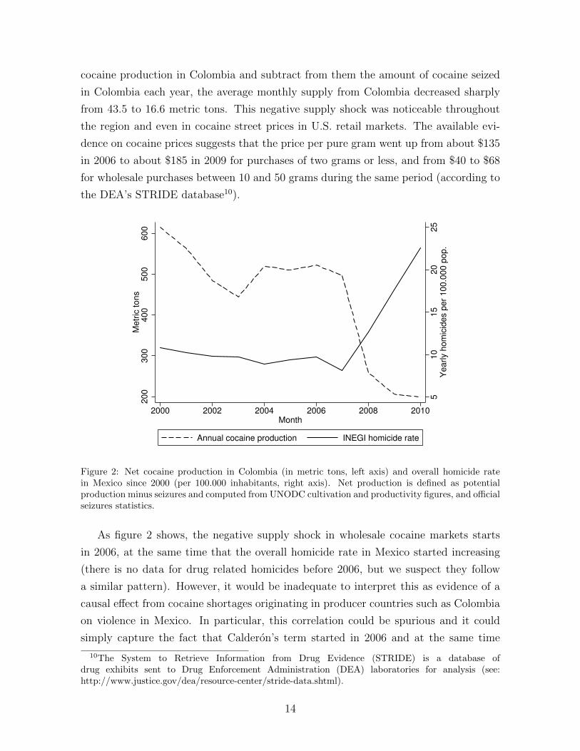
Figure 2: Net cocaine production in Colombia (in metric tons, left axis) and overall homicide ratein Mexico since 2000 (per 100.000 inhabitants, right axis). Net production is defined as potentialproduction minus seizures and computed from UNODC cultivation and productivity figures, and officialseizures statistics.
As figure 2 shows, the negative supply shock in wholesale cocaine markets starts
in 2006, at the same time that the overall homicide rate in Mexico started increasing
(there is no data for drug related homicides before 2006, but we suspect they follow
a similar pattern). However, it would be inadequate to interpret this as evidence of a
causal effect from cocaine shortages originating in producer countries such as Colombia
on violence in Mexico. In particular, this correlation could be spurious and it could
simply capture the fact that Calderon’s term started in 2006 and at the same time
10The System to Retrieve Information from Drug Evidence (STRIDE) is a database ofdrug exhibits sent to Drug Enforcement Administration (DEA) laboratories for analysis (see:http://www.justice.gov/dea/resource-center/stride-data.shtml).
14
Colombia modified its anti-drug strategy. The fact that violence in Mexico trends
upwards (especially in the north) since 2006, as well as seizures in Colombia, is what
led us to focus on high frequency variation after controlling for these trends. The
evidence obtained from monthly variation after flexibly controlling for trends is reliable
and can be interpreted as causal, since there is no reason to expect monthly variation
in seizures—which creates the variation in the supply of Colombian cocaine—to be
correlated with Calderon’s policies in Mexico or any other determinant of violence.
4 A model of scarcity and violence
In this section we present a model that guides and motivates our empirical analysis.
Our model adds structure to the intuition outlined above and provides a richer set of
implications to test. We start with a static model and then introduce some dynamic
elements to analyze the role of informal cooperation arrangements and their interaction
with enforcement and negative supply shocks in wholesale cocaine markets. Denote a
municipality by i, with i ∈ {1, 2, . . . , I}, and let si be its relative importance in cocaine
trafficking. Here, si is the share of total revenue from the cocaine trade that is disputed
in this municipality. Intuitively, municipalities close to U.S. entry points would have a
large si since most of the trafficking activities will take place there, and control of these
locations commands a larger share of total cocaine revenue.
Let Qs be the supply of Colombian cocaine. We simplify the analysis and assume
that Colombia is the only supplier of cocaine to Mexican cartels. This assumption does
not change our results as long as Peru and Bolivia (the other two cocaine producer
countries) do not have a perfectly elastic supply. We assume there is an iceberg cost,
1 − h, of trafficking, so that the final supply of cocaine reaching the U.S. is hQs.
This iceberg cost is shaped, among other things, by law enforcement and, especially,
interdiction policies in Mexico. Drugs are sold at a final price P , so that the total
revenue of the cocaine trade is hPQs. The demand for drugs is given by the inverse
demand function P d(hQs), which we assume is inelastic throughout. This assumption
implies that revenue increases as supply falls.
We assume that only a fraction 1−η of the total cocaine trade revenue is vulnerable
to appropriation by other cartels and must be contested and defended through violence.
Thus, η < 1 is a measure of how well protected property rights are, and it captures the
presence of reliable third party enforcement. The above assumptions imply that the
15
total drug revenue in municipality i that is vulnerable to appropriation by others is
(1− η)sihPQs. (1)
There are N cartels, indexed by c ∈ {1, 2, . . . , N}. Let Ni be the set of cartels
operating in municipality i. All cartels are rivals and we assume that within cartels
there is perfect cohesion. Thus, this model only focuses on inter-cartel violence, but
cartels without perfect cohesion or breakups can be easily incorporated by treating
them as different cartels.11 Our model assumes that cartels are unable to coordinate
their actions to restrict supply and take advantage of the low elasticity of demand to
increase profits. Also, we assume that cartels’ location is exogenous, which we think is
the right assumption when we look at high frequency variation in these markets. There
may be entry or exit of cartels, but this does not occur at monthly frequencies. Let Ic
be the set of municipalities in which a cartel operates. Finally, cartels are price takers
in our model.12 Even if there were some level of collusion, all we need is the degree of
competition to be high enough that residual demands are elastic while market demand
is inelastic.
The timing and full description of events is as follows:
1. Nature draws Qs randomly from some distribution F with support [0,∞). In our
empirical application the random nature of Qs is created by enforcement changes
in Colombia and month to month fluctuations in seizure rates.
2. Participants observe Qs. Each cartel buys Qsc units of cocaine at a price P s,
traffics it and sells it at a price P = P d(hQs), with P d being the inverse demand
function. There is a variable convex cost C(Qsc) of running the cartel operations
that satisfies the usual Inada conditions. At this point, the cartel has already paid
P sQsc to Colombian producers and C(Qs
c) in operating costs. The total revenue
generated by cocaine trafficking is hQsP . We assume demand is inelastic so that
revenue increases when Qs falls. We will show that the amounts determined at
this stage, Qsc and P s, have no incidence in the conflict or in the level of violence,
11We have also explored alternative models of moral hazard within cartels based on Acemoglu andWolitsky (2011). In these models, cartels use more violence and coercion against their own members toinduce effort when revenue is higher. Thus, intra-cartel violence could also increase as a consequence.
12The term cartel is therefore misleading, but for historical reasons it has been the name used byLatin American drug trafficking organizations, so we will stick to it. The powerful Colombian drugtrafficking organizations of the 1980s and 1990s (especially those from Medellın and Cali) startedcalling themselves carteles in order to emphasize that they were a few organizations that controlledthe whole trade, even though they did not collude to increase prices. The name stuck, and present-dayMexican organizations use the same name (see Gonzalbo, 2012).
16
but we still model this stage for the completeness of our analysis and to show that
the effects we explore arise after an equilibrium in this market.
3. In order to appropriate or defend revenue, cartels engage in conflict against each
other in the municipalities where they operate. They invest gc,i in weapons,
personnel, recruitment, and training in municipality i. By doing so, cartel c is
able to obtain a fraction qc,i of the total revenue being contested in municipality i,
where qc,i is determined endogenously according to the following contest succcess
function:13
qc,i =gc,i∑
c′∈Nigc,i
(2)
The aggregate level of drug related violence in municipality i is given by:
vi =∑c∈Ni
gc,i. (3)
4. Payoffs are realized. More specifically, cartel c obtains profits
− P sQsc − C(Qs
c) + ηhPQsc +∑i∈Ic
(qc,i(1− η)sihP
∑c
Qsc − gc,i
)(4)
Given the exogenous supply of drugs from Colombia, Qs, which is drawn from a
probability distribution, an equilibrium consists of market clearing prices and quantities
in the U.S., P (Qs) and Q(Qs), a market clearing price for cocaine supplied by Colombia
P s(Qs), and conflict strategies gc,i(Qs), such that they are a Nash equilibrium of the
sub-game in which cartels fight over the rents in municipality i. We now characterize
the equilibrium and some important properties.
The objective of cartels is to choose the amount of Colombian cocaine that they will
intend to traffic, Qsc, and their conflict strategies gc,i to maximize profits. This problem
is greatly simplified by noticing that the supply in the U.S. is simply hQs. Market
clearing implies that the final price of cocaine is given by:
P (Qs) = P d(hQs). (5)
Let R(Qs) be the total cocaine trade revenue generated by Mexican cartels. The
above observation shows that this is equal to R(Qs) = hP d(hQs)Qs, which increases
13A contest success function (CSF) is a technology wherein some or all contenders for resources incurcosts as they attempt to weaken or disable competitors (see Hirshleifer, 1991). Also see Skaperdas(1996) and Hirshleifer (1989) for a detailed explanation of the different functional forms of CSFs.
17
when Qs falls since demand is inelastic.14 In equilibrium, the revenue disputed in munic-
ipality i only depends on Qs, and is given by (1−η)siR(Qs). Thus, when choosing their
conflict efforts, cartels simply face a series of independent problems in each municipality
they operate. Cartel i’s maximization problem is given by:
maxgc,i
qc,i(1− η)siR(Qs)− gc,i. (6)
Notice that the choices over Qsc do not have to be taken into account when determining
conflict efforts, since market clearing conditions impose a particular structure on equi-
librium revenues, and because payments to Colombian cartels are treated as bygones
(i.e., they are not contested).15 The unique Nash equilibrium among cartels operating
in municipality i is symmetric and given by:
gc,i(Qs) =
|Ni| − 1
|Ni|2(1− η)siR(Qs). (9)
The above expressions fully characterize the level of violence in municipality i as
vi(Qs) =
|Ni| − 1
|Ni|(1− η)siR(Qs). (10)
This expression gives us our main proposition.
Proposition 1. Suppose demand is inelastic, so that revenue R(Qs) is decreasing in
Qs. A decrease in the Colombian supply of cocaine, Qs, increases revenue and leads to
more violence (on average) in all Mexico. The increase in violence is larger when:
14Mathematically, ∂ logR∂ logQs =
(1− 1
|εd|
), which is positive if and only if |εd| > 1, i.e., whenever
demand is inelastic.15 The model can still be fully solved as follows: Plugging the optimal choice of gc,i on the cartel’s
objective function yields
− P sQsc − C(Qsc) + ηhPQsc +∑i∈Ic
1
|Ni|2(1− η)sihP
∑c∈N
Qsc. (7)
Therefore, the optimal choice of Qsc ≥ 0 solves
P s + C ′(Qsc) ≥ ηhP +∑i∈Ic
1
|Ni|2(1− η)sihP, (8)
with equality if Qsc > 0. The convex cost C satisfying the Inada conditions was introduced so that itis possible for this equation to have a solution for more than one cartel. Otherwise one cartel– the onehaving presence on the best locations– would buy all drugs and the others would simply prey from it.We do not think this alternative situation is unrealistic, as many cartels are toll collectors and simplyprey on others, while not involved in cocaine trafficking directly. In fact, even with the convex costit is possible for some cartels to specialize in preying on others while not trafficking at all. Here, P s
and P are taken as given by the cartel. The equilibrium prices P (Qs), P s(Qs) are the only prices thatguarantee market clearing.
18
• Third party enforcement is absent or weak, so that η is small.
• si is higher. That is, in municipalities that are more important for cocaine traf-
ficking.
• There are more cartels |Ni|. In particular, the model predicts that violence would
increase only if there are at least two rival cartels operating in the same municipal-
ity. Violence would remain unchanged if there is only one or no cartels (although
there could be other sources of violence unrelated to the model).
Proof. The proof follows simply from differentiating equation 10 to obtain comparative
statics on the level of violence. The key observation is that expenditures on conflict
increase with total revenue in a municipality, and total revenue increases when supply
falls because demand is inelastic.
In our empirical application we will analyze if the data supports this proposition.
The first part of the proposition suggests that in the time series at the monthly level
we should observe that months with low cocaine production in Colombia due to higher
seizures should be months of higher violence in Mexico. There are several empirical
counterparts to si that one can think of, but in our empirical application we focus on
distance to entry points to the U.S. as an inverse measure of si. Clearly, municipalities
that are closer to U.S. entry points will be more important for trafficking and cartels
that control them would be able to extract more resources from the cocaine trade. Thus,
it seems reasonable to associate these municipalities with a high value of si. Our model
not only predicts that we should find a relation between scarcity and violence on average;
there should also be a gradient, with violence increasing more in municipalities near U.S.
entry points, and with the effect fading out as we move away from the frontier. Finally,
the model suggests that it “takes two to tango”. That is, violence should increase as
a consequence of scarcity only in places with at least two cartels. Moreover, as the
number of cartels operating in a municipality keeps increasing, the model predicts that
scarcity will have a bigger effect on violence. We will test this implication by estimating
the differential effect of cocaine shortages in municipalities with different numbers of
cartels present at the time of the supply shock.
Before continuing with the dynamic extension of the model, we make some comments
on its setup. First, note that shocks to Colombian supply Qs are exogenous, as they
will be in our econometric application. Second, note that si is an exogenous variable
that captures, in a reduced form, how intensively drug trafficking uses routes, labor and
resources in general from municipality i. The assumption is that in municipalities that
19
are important for the cocaine trade, more revenue will be disputed. In a more complete
model one would like to determine si from the production structure and technology,
and study how this relates to more rents being present in a municipality. However, this
suffices for the purposes of our model.16 In our model, we think of cartels as trafficking
cocaine across the U.S. border, so si does not capture the potential of a municipality
for consumption. This interpretation could be easily accommodated, and, in fact, it
would not change our interpretation or results, but the main source of profits from the
cocaine trade are exports to the U.S. (see Kilmer et al., 2010), so we stick to the idea
of cartels as smugglers that take drugs to the U.S.
Our model also assumes that cartels fight over the share of revenue that is vulnerable
to appropriation. What they fight over is revenue and not profits, because payments
to Colombian cartels are sunk costs. Thus, cartels are the full residual claimants of the
rents they appropriate and protect from others. A slightly more complex version of our
model would yield the same results as long as there is no perfect risk sharing between
cartels and suppliers in Colombia. For instance, if cartels and suppliers were able to
establish complex contracts, one could have a situation in which cartel payments to
suppliers depend on its conflict success, and cartels could end up fighting over profits,
rather than revenue. We believe that the absence of third party enforcement precludes
these vertical relationships, and payments to Colombian suppliers can be treated as
bygones.17 Operating costs, C, are also bygones. This convex cost simply smooths the
equilibrium and guarantees that it is possible to have more than one cartel operating
in the cocaine trade and not simply preying on others. (For details, see footnote 15).
We assume an inelastic demand so that revenue increases as supply tightens. This is
widely believed to be the case for drugs, especially for cocaine, since it is a psychoactive
substance that is highly addictive: consumers buy their daily dose regardless of the
market price, which means that demand does not respond largely to prices. Becker et
al. (2006) mention an elasticity of less than 1 for most drugs, with a central tendency
towards 1/2, especially in the short run. The relevant value for our model is the short
run elasticity of demand, which is considerably smaller than in the long run, since a
16For instance, one could follow Dell (2013) and pose a model in which si is determined by the roadnetwork and enforcement in municipalities, and where the objective of cartels is to transport drugs toentry points to the U.S. minimizing transportation costs. In this model, municipalities that are alongthe faster drug routes would command a high si because they are helpful for production, and providemore rents to the cartels controlling them.
17However, other alternative models yield similar results. In Mejia and Restrepo (2013) scarcityincreases conflict over the control of routes as long as the elasticity of demand is larger than theelasticity of substitution between drugs and routes. Castillo (2013) also provides conditions over theelasticity of demand that make enforcement increase profits.
20
short term spike in prices affects only a fraction of the present value of payments a
consumer has to make to keep a drug habit (see Becker and Murphy (1988) for the full
theoretical argument and Becker et al. (1994) for evidence from cigarette consumption).
Early attempts to measure the elasticity of demand of drugs estimated inelastic
demands but focused mainly on marijuana and heroin. See, for instance, Nisbet and
Vakil (1972) for Marijuana among UCLA students, Roumasset and Hadreas (1977) for
heroin in Oakland, and Silverman and Spruill (1977) for heroin in Detroit. Wasserman
et al. (1991) and Becker et al. (1994) find demand elasticities between -0.4 and -0.75
for cigarette consumption in the short run, which supports the idea that the demand
for addictive substances is price inelastic. For cocaine, more recent studies typically
estimate inelastic demands as well. Bachman et al. (1990) find no evidence of increas-
ing availability of cocaine leading to more consumption among high school students.
DiNardo (1993) finds no link between consumption and variation in enforcement. Both
studies are consistent with an inelastic demand. Saffer and Chaloupka (1999) estimate
a price elasticity of demand for cocaine of -0.28 (their estimates for alcohol and heroin
are -.3 and -.98 respectively). Caulkins (1995) reaches a different conclusion using the
fraction of arrestees testing positive for drugs to construct a measure of the elasticity
of demand for cocaine and heroin: he finds elasticities for cocaine between -1.5 and -
2.0. However, his methodology relies on the assumption that prices do not affect arrest
rates, as well as other modeling choices, and only identifies a local elasticity among
a particular group. Despite this single work that contradicts our assumption, we will
maintain that cocaine demand is inelastic, as it is supported by our results. If demand
were elastic, cocaine shortages would decrease violence, which is the opposite of what
we actually find.
Finally, the contest success function in equation 2 is standard in the conflict lit-
erature and is not essential for our results (see Skaperdas (2002) for more on contest
success functions). All we need for our results is that the function be concave in gc,i,
satisfy the Inada conditions, and exhibit either increasing differences in the vector of
gc,i, or small cross-derivatives if they are negative. This implies that the stakes at play
increase violence, which is what one would intuitively expect. The conflict function is
a reduced form representation of all strategies available to cartels to appropriate drug
rents. For instance, cartels can act as toll collectors, and extort other cartels oper-
ating in municipality i that have cash, cocaine, or assets at this municipality due to
its trafficking importance. They could also fight for turf in order to use routes and
labor for their trafficking activities. They could prey on each other by violently steal-
ing cash, weapons, assets or other resources, or they could eliminate competition from
21
key municipalities, which could increase their market share. There are also non-violent
ways in which cartels could compete for the rents of the cocaine trade obtained from
controlling municipality i. For instance, they could bribe public officials, or even en-
gage in the provision of goods to the community to gain popular support. We are not
modeling these alternatives, which intuitively are more relevant in a longer planning
horizon than in the monthly frequency we are considering in this paper. Using violence
is an equilibrium even if these alternatives are available, and intuitively, it is the first
order margin of response in the short run, when opportunities to prey become available
and rapacity intensifies.
Having clarified these aspects of the model we move to a dynamic setup. We have
repeatedly argued that our empirical strategy measures the response of violence to
high frequency supply shocks in order to make sure that we do not measure spurious
correlations. Thus, our model must also show that the results of proposition 1 hold
when supply shocks last for a short time. We will follow Rothemberg and Saloner
(1986), Abreu et al. (1990) and Castillo (2013). The dynamics allow us to focus on
Subgame Perfect Equilibria (SPE) of the repeated game in which cartels fight each
other for the control of revenue. We think this is a natural extension because in a world
without third party enforcement, participants rely not only on violence, but also on
informal arrangements sustained under the threat of retaliation, and SPE captures this
possibility. The dynamic model allows us to understand the effect of supply shortages
when such informal cooperative arrangements are in place, and more importantly, how
they interact when government policies are aimed at capturing or killing cartel leaders,
greatly reducing the scope of such arrangements.
In particular, we are interested in understanding the effect of enforcement during
Calderon’s war on drugs, and how it affected inter-cartel conflict. During our period
of analysis, the war on drugs was spearheaded by the PAN party. As shown by Dell
(2012), municipalities with PAN mayors were more likely to crack down on the drug
trade. Calderon’s strategy did not take the form of increasing seizures. In fact, cocaine
seizure rates in Mexico varied little over time before and after Calderon took office. The
real focus of Calderon’s war on drugs was on arresting drug kingpins (see Guerrero,
2011a). This task was easier in municipalities with PAN mayors or large PAN support.
Thus, we model the role of PAN by letting municipalities have an idiosyncratic arrest
probability ai which is higher when there is popular support for PAN actions. There are
many other ways in which enforcement could affect our model of inter-cartel violence.
For instance, η could be municipality-specific, with higher enforcement municipalities
having a lower η, because a tighter enforcement of drug markets destroys property
22
rights. Or h could be lower in municipalities with more enforcement if this is directed
at seizing drugs, but as we argued above, we do not think this is what the anti-drug
strategy on Mexico has focused on, at least during our period of analysis.
In the dynamic model, the same game described above is played repeatedly, with an
independent draw of Qst in each period. At the end of the period, nature reveals which
cartel leaders are arrested. A cartel leader in municipality i is arrested with probability
ai and then replaced by a new one. We assume leaders take all decisions maximizing the
cartel profits with their own discount rate (1−ai)β, and not with the “market” discount
rate β they would have if the incentives of the leaders and the cartel “shareholders”
were aligned. In other words, arrests make cartel leaders behave more impatiently than
they otherwise would, so, unlike what happens with traditional firms, the discount rate
of the CEO—the leader—matters. The idea is that once a cartel leader is arrested
or killed, the next leader cannot credibly compensate him for long term investments,
which also stems from the lack of enforceable contracts in environments without third
party enforcement. An alternative is to assume that with probability ai the cartel is
dismantled in municipality i, but casual observation suggest that Calderon’s policy has
been mostly to behead leaders who are quickly replaced (at least in the short run),
which fits our model well. It is possible that some cartels will be dismantled on the
long run, as suggested by some supporters of Calderon’s policies, but we believe this is
not the case at the monthly frequency we are focusing on.
Formally, at time t0 a cartel maximizes
Et0
∑t≥t0
βt−t0(1−ai)t−t0[−C(Qs
c,t)− P st Q
sc,t + ηhPtQ
sc,t +
∑i∈Ic
(qc,i,t(1− η)sihPtQst − gc,i,t)
],
(11)
where we have added a time subscript to all variables that change in time. The intra-
period timing is as defined above. To simplify things we assume that cartels cannot
condition their actions on past choices of quantities or cannot punish by demanding
different quantities. Also, we assume that actions in municipality i can only be condi-
tioned on past actions in this municipality. This greatly simplifies the characterization
of Subgame Perfect Equilibria, while still allowing for some natural degree of coop-
eration maintained through the threat of retaliation. This assumption implies that
quantities will be chosen as in the static problem, and we can treat the conflict in each
municipality as a separate problem. For all cartel leaders in municipality i, we have a
repeated game that we can study separately. Just as in the static problem, the amount
paid for drugs P st Q
2c,t, the cost of running the cartel operation C(Qs
c,t), and the revenues
23
that are not subject to appropriation ηhPtQsc,t are bygones. Thus, during each period
they choose gc,i,t to maximize their expected payoffs
Et0
∑t≥t0
βt−t0(1− ai)t−t0qc,i,t(1− η)siR(Qst)− gc,i,t. (12)
The unique Markov Perfect Equilibirum (MPE) of the dynamic game coincides with
the repeated static equilibrium described above. However, we are interested in other
Subgame Perfect Equilibria (SPE) which allow for more cooperation and punishments.
Since the contribution of our paper is not at the theoretical level, we focus on the
simplest SPE that allows for some degree of self-enforcing commitment. In particular,
let gN(Qs) be the symmetric static Nash equilibrium when supply is Qs, which coincides
with the solution to the static model. We consider a recursive equilibrium with all
cartels spending gC(ai, Qs) ∈ [0, gN(Qs)), and reverting to gN(Qs) if anyone deviates.
This may not be the most cooperative SPE but it is the simplest one and it helps us
illustrate our point. The equilibrium is characterized in the following proposition:
Proposition 2. Suppose demand is inelastic, so that R(Qs) is decreasing in Qs. The
equilibrium sustaining more cooperation through reversion to the static Nash MPE is
recursive and involves gc,i = gC(ai, Qs) ∈ [0, gN(Qs)). The function gC satisfies the
following properties:
• Suppose revenue is unbounded from below. Then, for Qs ≥ Q(ai), gN(ai, Qs) = 0.
Thus, for any arrest probability, there is no violence if revenue is sufficiently low.
Moreover, Q(ai) is increasing in ai.
• Suppose revenue is unbounded from above. Then gN(ai, Qs) > 0 for Qs sufficiently
small, even if β(1 − ai) → 1. If revenue is bounded as Qs → 0, then a fully
cooperative equilibrium with gN(ai, Qs) = 0 ∀Qs can be sustained if β(1−ai) > β,
for some β.
• gN is increasing in ai, decreasing in Qs and the cross partial is negative. Thus,
supply shortages have a larger impact on violence in municipalities with a higher
arrest rate, specially in those that are important for drug trafficking.
Proof. The proof follows Rothemberg and Saloner (1986), and is presented in appendix
B.
The key intuition from this proposition is that in the absence of third party en-
forcement, there is room for some de facto protection of property rights created by the
24
threat of future retaliation. In fact, cartels may behave less violent if they know that
predatory behavior would trigger a reversion to the violent and costly static Nash equi-
librium. Notice that when ai is low and β high, an equilibrium with no violence can be
sustained, where predation does not occur on the equilibrium path. This is a variant of
the Folk theorem. However, as the effective discount rate decreases, participants value
the future less and some level of predation has to be allowed in the SPE, especially when
supply is tight and revenue is high. The reason is twofold: the temptation to prey is
higher, and future revenues are also smaller on average, so future retaliation seems less
severe. The arrest rate makes future punishments look even less severe by reducing
the value of future payoffs, and an even larger level of violence must be allowed in the
present when supply is tight. This logic explains the negative cross partial derivative
of the function gC(ai, Qs). The allowed level of violence keeps down the incentives to
deviate because it makes harder for other cartels to prey on others, given their current
level of expenditure on weapons; but also because the incremental gain from exerting
more violence is reduced.
One important point from the proposition is that informal arrangements based on
dynamic threats are not enough to eliminate the consequences of supply shortages on
violence as long as the future is significantly discounted. Thus, scarcity leads to vio-
lence even in the presence of informal cooperative arrangements because of the reasons
outlined above. Informal arrangements are not only limited by the fact that revenue
can be high today and small in the future, but also by a higher discounting among
participants created by other policies.
The empirical content of this proposition is that supply shocks should have a larger
effect in northern municipalities with high turnover of cartel leaders. Following Dell
(2013), the effect of supply shortages should be especially large in the north, and in
places where there is massive support for the PAN, which is the party that spearheaded
the war on drugs in Mexico. In these municipalities there is more cooperation with
federal authorities and Calderon’s policy of arresting or killing cartel leaders decreases
the effective discount rate more than in less pro-PAN municipalities.
The rest of the paper describes our empirical work in which we test the main pre-
dictions of our model and investigate the role of scarcity mediated by several factors,
including the number of participants, the importance of the location for the commod-
ity trade, and enforcement in the form of a higher probability of arrests or killing of
participants.
25
5 Empirical strategy and data
In order to test our model, we need exogenous supply shocks to proxy for changes in Qs.
The Mexican setting, in which cocaine trafficked by cartels is purchased from Andean
countries, suggests that we can use fluctuations in the Colombian supply of cocaine
as our source of exogenous variation in scarcity. Though cartels may compensate by
purchasing more cocaine from other sources, it would still be the case that final prices
would rise by more than the fall in quantities as long as demand is inelastic.
To get a clean identification of the effect of scarcity, we focus on high frequency
supply shocks at the monthly level. Monthly supply from Colombia is constructed by
taking annual production and transforming it to monthly figures, and then subtracting
monthly seizures. Using high frequency variation in the Colombian supply also has
additional advantages. First, since we remove the low frequency component, long term
trends that are spuriously correlated do not confound our estimates. More specifically,
there is a downward trend in Colombian supply and an upward trend in crackdowns in
Mexico since president Calderon took office at the end of 2006. This implies that there
is a correlation at the yearly level that is likely to be spurious. The key identifying
assumption is that this correlation breaks down at higher frequencies once trends are
partialed out. The resulting monthly variation is arguably exogenous to other phenom-
ena determining violence in Mexico or other secular trends. The second advantage is
that this variation is mostly driven by changes in seizures, since monthly production
by construction does not vary a lot at this high frequency. This can be seen from the
high correlation between seizures and net supply in figure 3. Thus, our variation does
not reflect the possibility that supply may be responding to changes in the Mexican
market that could directly affect violence. In fact, results using seizures directly as the
independent variable are very similar, suggesting that all our estimations are driven by
the monthly variation in seizures in Colombia. Finally, the short run nature of these
shocks implies that prices are more responsive, since there is less room for substitution,
and other source countries cannot rapidly increase their supply.
These advantages of using high frequency shocks allow us to estimate the causal
effect of short run fluctuations in scarcity due to exogenous conditions, and obtain a
clean identification of its effect on violence. We are confident that the month to month
variation in seizures that we exploit is mostly driven by luck (i.e., one military or police
operation turned out to be successful in detecting and interdicting a cocaine shipment),
or by factors that are exogenous to Mexico (i.e., politics or funding in Colombia). Figure
3 plots the monthly variation in the Colombian supply from 2000 to 2010 after removing
26

time trends using a cubic polynomial (in the months) and year dummies.
−.6
−.4
−.2
0.2
.4P
erc
en
tag
e s
eiz
ed
−3
0−
20
−1
00
10
Me
tric
to
ns
2007m1 2008m1 2009m1 2010m1 2011m1Month
Monthly supply shocks Seizure rate (inverse)
Figure 3: The figure shows the production of Colombian cocaine at a monthly level net of seizures (inmetric tons, left axis). We plot the residual component after partialing out a cubic polynomial in themonth. We plot the inverse of the monthly seizure rate on the right axis (data from the ColombianNational Police).
We study the time series effect of these shocks on violence by estimating the model
hi,t = λi + βct + St(γ) + θX ′i,t + εi,t (13)
where hi,t is a monotone transformation of the homicide rate in municipality i at time
t, ct is the net cocaine production in Colombia in month t, and εi,t is an error term.
The term St(γ) =∑3
n=0 γntn + yt includes both a cubic polynomial and year dummies
that control flexibly for time trends. It therefore guarantees that we exploit only the
high frequency component of cocaine production plotted in figure 3, which is driven
by the exogenous variation in seizures in Colombia. In particular, this term eliminates
all year to year variation and smooths longer term variation that may confound our
estimates. Our results do not change if instead of a cubic polynomial we use a quadratic
or quartic polynomial to detrend our data (see appendix A). Finally, X ′it is a vector with
additional controls. This is essentially a time series exercise which exploits efficiently
all the municipality data and controls for compositional changes. Our model suggests
that β < 0, and we focus on this hypothesis in this case. The identifying assumption is
that the high frequency component of cocaine production in Colombia, ct, is orthogonal
27
to εi,t once time trends are flexibly controlled for. As we argued above, we believe this
is the case at the monthly level.
To investigate the other predictions of our theoretical model, we estimate regressions
of the form
hi,t = λi + δt + βctαi + αiSt(γ) + θX ′i,t + εi,t (14)
for different interaction variables αi. In these models we test for heterogeneous ef-
fects of supply shocks on violence depending on municipality characteristics. Since in
these models we focus on the differential effects of scarcity depending on municipal-
ity characteristics, we control for a full set of month dummies. The interaction term
ctαi provides within municipality variation that allows us to identify the heterogeneous
effect of cocaine shortages on violence. We explore heterogeneity by distance to U.S.
entry points, which is our proxy for a municipality’s importance in the cocaine tarde,
si. On top of these interactions we will add another layer and investigate heterogeneity
by the number of cartels operating in a municipality and by support for the PAN party.
The conditions required to give our estimates a causal interpretation will be discussed
when we present each set of results. One key aspect is that the term αiSt(γ) (with
St(γ) =∑3
n=0 γntn + yt, just as in equation (13)) flexibly controls for differential trends
and year to year variation in homicides that varies systematically with the interaction
variable αi. This gives us a sharper identification, since the effect of the interaction
is obtained from a comparison between short term fluctuations in violence in munici-
palities with different αi during a supply shock. Before moving to our estimation we
present our data.
5.1 Data
Our main dataset is a monthly panel of 2,438 Mexican municipalities from December
2006 until December 2010. Our dependent variables are measures of the monthly homi-
cide rate in a municipality. We use two main sources. Our first source is the monthly
homicide rate from INEGI (Mexico’s Instituto Nacional de Estadıstica y Geografıa18).
This data is available from 1990 to 2010 and includes all homicides (not only those re-
lated to drug trafficking). Our second source is the data on drug related homicides that
was published by the Mexican Presidency, and includes the number of monthly casual-
ties from December 2006 until December 2010.19 This dataset only includes homicides
18The data can be downloaded from INEGI’s website, www.inegi.org.mx19Unfortunately, the new Mexican government of Enrique PeA±a Nieto, who took office in December
2012, stopped publishing these homicide rates, which were previously available online.
28
that, according to local authorities, had a relation with the illegal drug trade. Drug
related homicides are divided into three broad categories: (1) executions, which involve
targeted assassinations by DTOs; (2) confrontations, which are the result of battles
either between competing DTOs or between DTOs and government authorities; and
(3) aggressions, which are targeted homicides caused by DTOs attacking government
forces. However, there is an ongoing debate about the reliability of this classification.20
Thus we also show all of our results using the INEGI measure of the overall homicide
rate. Another advantage of the INEGI measure is that it covers a longer time period,
which will be useful in some of our empirical exercises. Finally, in our robustness ex-
ercises we also use the homicide rates reported by the SINAIS21, which gathers the
information from public health records.
We compute monthly homicide rates (normalized at a yearly basis) using census
population counts. Given the high skewness in homicide rates, we follow literature on
crime and use a logarithmic transformation. However, this is problematic at a monthly
frequency because there is a high probability of having no homicides. We address this
issues by estimating our models with different transformations of the homicide rate. In
particular, for any homicide rate we use
hi,t = log(ri,t + p90), (15)
with p90 being the 90th percentile of the homicide rate in our sample. This transforma-
tion is increasing in ri,t, and is well defined. Our results hold for a variety of alternative
transformations shifting the homicide rates by different amount (such as the 50th or the
10th percentile); for Poisson or negative binomial models; or for a dummy that takes
the value of 1 when there is a homicide recorded (see appendix A). The reason why
we choose the 90th percentile in our preferred estimate is that it is the transformation
that results in errors that are closest to normal.
To interpret results obtained with this transformation, notice that the approxima-
tion
∆ log(ri,t + p90) ≈ ri,tri,t + p90
∆ log ri,t, (16)
holds. The sample average of rit+p90rit
is 10.07 for the INEGI homicide rate and 21.12
for drug related homicides. Thus, an easy rule of thumb to transform our estimates
into log points is to multiply them by 10 when the dependent variable is the INEGI
homicide rate and by 20 when the dependent variable is the drug related homicide
20For some of the articles that criticize the data, see Lizarraga (2012) and Proceso (2012).21Sistema Nacional de Informacion en Salud - http://www.sinais.salud.gob.mx/
29
rate.22 We will use this simple rule of thumb when discussing the economic significance
of our results. Of course, the approximation does not hold for larger changes in policies
and in those cases we will compute the exact implied changes in homicides rates under
counterfactual scenarios.
As explained above, we explore the effect of scarcity mediated by the trafficking
importance, the number of cartels and the political power of the PAN party. We use
the distance to the nearest U.S. entry point as our proxy for trafficking importance.
This is computed as the distance from the centroid of each municipality to the closest
U.S. entry point. The centroids are obtained from INEGI and the entry points from
Google Earth. To explore heterogeneity by the number of participants or cartels, we
use the measure of presence of drug cartels proposed by Coscia and Rıos (2012), who,
based on web content such as blogs and news, build a yearly panel that tells whether
each cartel was present in each municipality during each year. The dataset covers the
period from 1990 until 2010 and contains information about the seven most important
Mexican drug cartels in this period (Cartel de los Hermanos Beltran Leyva, Familia
Michoacana, Cartel del Golfo, Cartel de Juarez, Cartel de Sinaloa, Cartel de Tijuana
and Los Zetas), as well as about the presence of other smaller DTOs. Finally, to explore
heterogeneity by PAN political power, we use historical voting shares for PAN municipal
mayors in the municipality.
Our variation in scarcity comes from high frequency changes in the supply of Colom-
bian cocaine induced by interdiction efforts. We construct a monthly measure of the net
supply of Colombian cocaine as follows: First, we compute annual cocaine production
figures from UNODC and convert them to a monthly basis by extrapolating with a
third-order spline of the logarithm of production. We then subtract from each month’s
estimated production cocaine seizures within Colombia during that month. Seizures
are obtained from data provided by the Colombian Ministry of Defense covering all
months in our sample (the detrended component of these series was presented in figure
3). When giving an idea of the size of our estimates, we will compute the effect of a
10mt decrease in the monthly net Colombian supply of cocaine. This is roughly the
standard deviation of this series and about 1/5th of the average monthly production of
Colombian cocaine in 2006.
We also include some additional municipality covariates in some of our estimations,
all of which were obtained from INEGI. First, we include municipality income, which
varies at the yearly level. We also include some measures of state presence, which include
22The corresponding adjustment factors for executions, confrontations and aggressions are 19.8,47.84 and 32.30, respectively.
30
social security personnel per capita (both from the Mexican Institute or Social Security
(IMSS) and from the Instituto de Seguridad y Servicios Sociales de los Trabajadores
del Estado (ISSSTE)) and middle and high school teachers per capita. Again, these
variables only vary at a yearly level, so they control for longer term socioeconomic
phenomena when added as covariates. In our time series exercises we control for the
INEGI national unemployment rate at the monthly level and for the IGAE, a measure
of economic activity that is available on a monthly basis, and which is highly correlated
with the GDP.
Table 1 summarizes our data. The table presents statistics separately for all Mex-
ico, for the 40% closest municipalities to U.S. entry points (quintiles 1 and 2 of the
distance), and for the 20% closest municipalities (the first distance quintile). Note that
the Mexican population is skewed towards municipalities that are closer to the U.S.:
The first distance quintile includes 24.9% of the national population, and quintiles 1
and 2 include 60%. Many of our results focus on these two quintiles, which include the
majority of the Mexican population.
The top panel summarizes time varying variables. For each group it reports statis-
tics for all months or for the growth of the variable between 2007 and 2010 (recall that
our first month is December 2006). The bottom panel reports fixed municipality char-
acteristics. As the table shows, the north of Mexico (Quintiles 1 and 2) is more violent
as measured by the INEGI homicide rate and drug related homicides. Not only were
quintiles 1 and 2 more violent in 2007, but violence also increased disproportionally in
the north. The homicide rate in Mexico increased by 98 log points, while it increased by
119 log points in quintiles 1 and 2, and by 164 log points in the first quintile. A similar
pattern emerges for drug related crimes. Interestingly, the data shows that the vast
majority of homicides in the north are drug related, whereas homicides in other areas
of the country are less so. In consistency with the intuition that the north of Mexico
is more important for cocaine trafficking, we see a higher cartel presence in quintiles 1
and 2 than in the country as a whole. In particular, the average number of cartels per
municipality was 0.86 in the first quintile, and 0.47 in Mexico as a whole. Furthermore,
most homicides in our data took place in these two quintiles: they include 55% of all
homicides committed in 2006, and 75% of homicides committed in 2010. The growth
in cartel presence during this period has been more homogeneous along the country.
Finally, northern municipalities are historically more likely to support the PAN, as
captured by the PAN vote share during 1990-2000.
31
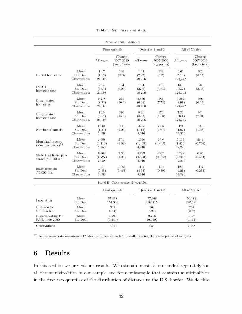
Table 1: Summary statistics.
Panel A: Panel variables
First quintile Quintiles 1 and 2 All of Mexico
All yearsChange
All yearsChange
All yearsChange
2007-2010 2007-2010 2007-2010(log points) (log points) (log points)
INEGI homicidesMean 1.17 169 1.04 123 0.60 103
St. Dev. (10.2) (9.8) (7.92) (6.7) (5.13) (5.17)Observations 24,108 48,216 120,442
INEGIMean 25.4 164 16.4 119 14.8 98
homicide rateSt. Dev. (56.7) (6.05) (37.8) (5.35) (35.2) (3.33)
Observations 24,108 48,216 120,345
Drug-relatedMean 0.778 221 0.556 181 0.292 166
homicidesSt. Dev. (8.21) (10.1) (6.06) (7.78) (3.91) (6.15)
Observations 24,108 48,216 120,442
Drug-relatedMean 16.9 216 8.81 176 7.28 161
homicide rateSt. Dev. (65.7) (15.5) (42.2) (15.8) (36.1) (7.94)
Observations 24,108 48,216 120,345
Mean 0.861 61 .695 75.6 .471 78Number of cartels St. Dev. (1.27) (2.03) (1.19) (1.67) (1.02) (1.33)
Observations 2,458 4,916 12,290
Municipal incomeMean 2,658 27.1 1,960 27.6 2,136 26.6
(Mexican pesos)23St. Dev. (1,113) (1.69) (1,403) (1.44%) (1,420) (0.768)
Observations 2,458 4,916 12,290
State healthcare per-Mean 0.969 2.33 0.793 2.67 0.748 0.95
sonnel / 1,000 inh.St. Dev. (0.727) (1.05) (0.693) (0.877) (0.705) (0.584)
Observations 2,458 4,916 12,290
State teachersMean 13 0.785 11.5 -1.15 12.3 -1.5
/ 1,000 inh.St. Dev. (2.65) (0.468) (4.63) (0.39) (4.21) (0.253)
Observations 2,458 4,916 12,290
Panel B: Cross-sectional variables
First quintile Quintiles 1 and 2 All of Mexico
PopulationMean 57,438 77,906 50,182
St. Dev. 154,383 332,115 225,021
Distance to Mean 331 508 758U.S. border St. Dev. (184) (220) (267)
Historic voting for Mean 0.280 0.256 0.176PAN, 1990-2000 St. Dev. (0.140) (0.149) (0.161)
Observations 492 984 2,458
23The exchange rate was around 12 Mexican pesos for each U.S. dollar during the whole period of analysis.
6 Results
In this section we present our results. We estimate most of our models separately for
all the municipalities in our sample and for a subsample that contains municipalities
in the first two quintiles of the distribution of distance to the U.S. border. We do this
32
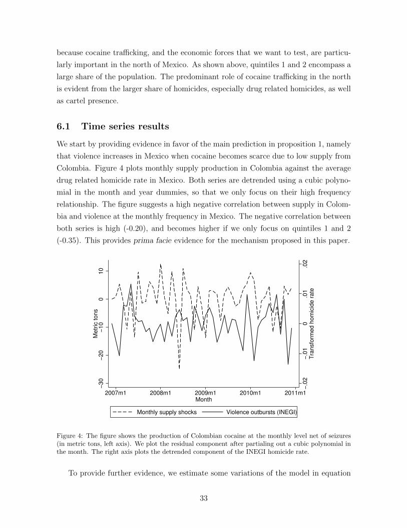
because cocaine trafficking, and the economic forces that we want to test, are particu-
larly important in the north of Mexico. As shown above, quintiles 1 and 2 encompass a
large share of the population. The predominant role of cocaine trafficking in the north
is evident from the larger share of homicides, especially drug related homicides, as well
as cartel presence.
6.1 Time series results
We start by providing evidence in favor of the main prediction in proposition 1, namely
that violence increases in Mexico when cocaine becomes scarce due to low supply from
Colombia. Figure 4 plots monthly supply production in Colombia against the average
drug related homicide rate in Mexico. Both series are detrended using a cubic polyno-
mial in the month and year dummies, so that we only focus on their high frequency
relationship. The figure suggests a high negative correlation between supply in Colom-
bia and violence at the monthly frequency in Mexico. The negative correlation between
both series is high (-0.20), and becomes higher if we only focus on quintiles 1 and 2
(-0.35). This provides prima facie evidence for the mechanism proposed in this paper.
−.0
2−
.01
0.0
1.0
2T
ran
sfo
rme
d h
om
icid
e r
ate
−3
0−
20
−1
00
10
Me
tric
to
ns
2007m1 2008m1 2009m1 2010m1 2011m1Month
Monthly supply shocks Violence outbursts (INEGI)
Figure 4: The figure shows the production of Colombian cocaine at the monthly level net of seizures(in metric tons, left axis). We plot the residual component after partialing out a cubic polynomial inthe month. The right axis plots the detrended component of the INEGI homicide rate.
To provide further evidence, we estimate some variations of the model in equation
33
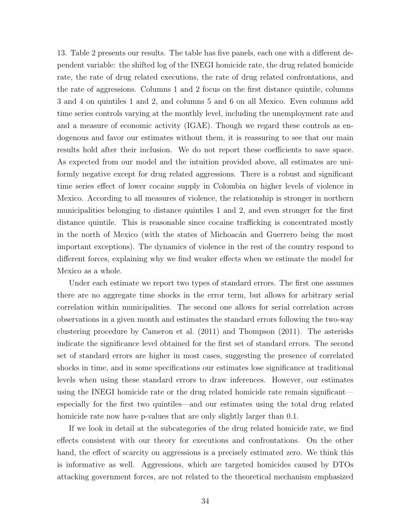
13. Table 2 presents our results. The table has five panels, each one with a different de-
pendent variable: the shifted log of the INEGI homicide rate, the drug related homicide
rate, the rate of drug related executions, the rate of drug related confrontations, and
the rate of aggressions. Columns 1 and 2 focus on the first distance quintile, columns
3 and 4 on quintiles 1 and 2, and columns 5 and 6 on all Mexico. Even columns add
time series controls varying at the monthly level, including the unemployment rate and
and a measure of economic activity (IGAE). Though we regard these controls as en-
dogenous and favor our estimates without them, it is reassuring to see that our main
results hold after their inclusion. We do not report these coefficients to save space.
As expected from our model and the intuition provided above, all estimates are uni-
formly negative except for drug related aggressions. There is a robust and significant
time series effect of lower cocaine supply in Colombia on higher levels of violence in
Mexico. According to all measures of violence, the relationship is stronger in northern
municipalities belonging to distance quintiles 1 and 2, and even stronger for the first
distance quintile. This is reasonable since cocaine trafficking is concentrated mostly
in the north of Mexico (with the states of Michoacan and Guerrero being the most
important exceptions). The dynamics of violence in the rest of the country respond to
different forces, explaining why we find weaker effects when we estimate the model for
Mexico as a whole.
Under each estimate we report two types of standard errors. The first one assumes
there are no aggregate time shocks in the error term, but allows for arbitrary serial
correlation within municipalities. The second one allows for serial correlation across
observations in a given month and estimates the standard errors following the two-way
clustering procedure by Cameron et al. (2011) and Thompson (2011). The asterisks
indicate the significance level obtained for the first set of standard errors. The second
set of standard errors are higher in most cases, suggesting the presence of correlated
shocks in time, and in some specifications our estimates lose significance at traditional
levels when using these standard errors to draw inferences. However, our estimates
using the INEGI homicide rate or the drug related homicide rate remain significant—
especially for the first two quintiles—and our estimates using the total drug related
homicide rate now have p-values that are only slightly larger than 0.1.
If we look in detail at the subcategories of the drug related homicide rate, we find
effects consistent with our theory for executions and confrontations. On the other
hand, the effect of scarcity on aggressions is a precisely estimated zero. We think this
is informative as well. Aggressions, which are targeted homicides caused by DTOs
attacking government forces, are not related to the theoretical mechanism emphasized
34
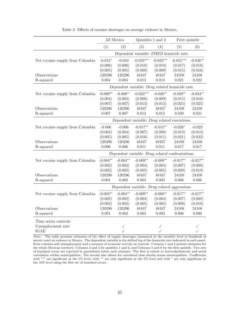
Table 2: Effects of cocaine shortages on average violence in Mexico.
All Mexico Quintiles 1 and 2 First quintile
(1) (2) (3) (4) (5) (6)
Dependent variable: INEGI homicide rate.
Net cocaine supply from Colombia -0.012∗ -0.010 -0.035∗∗∗ -0.033∗∗∗ -0.051∗∗∗ -0.046∗∗
(0.006) (0.006) (0.010) (0.010) (0.017) (0.018)(0.005) (0.005) (0.008) (0.009) (0.015) (0.016)
Observations 120296 120296 48167 48167 24108 24108R-squared 0.004 0.004 0.013 0.013 0.021 0.022
Dependent variable: Drug related homicide rate.
Net cocaine supply from Colombia -0.009∗∗ -0.008∗∗ -0.023∗∗∗ -0.020∗∗ -0.039∗∗ -0.034∗∗
(0.004) (0.004) (0.008) (0.009) (0.015) (0.016)(0.007) (0.007) (0.013) (0.013) (0.025) (0.025)
Observations 120296 120296 48167 48167 24108 24108R-squared 0.007 0.007 0.012 0.012 0.020 0.021
Dependent variable: Drug related executions.
Net cocaine supply from Colombia -0.006 -0.006 -0.017∗∗ -0.015∗∗ -0.026∗ -0.023(0.004) (0.004) (0.007) (0.008) (0.013) (0.014)(0.005) (0.005) (0.010) (0.011) (0.021) (0.022)
Observations 120296 120296 48167 48167 24108 24108R-squared 0.006 0.006 0.011 0.011 0.017 0.017
Dependent variable: Drug related confrontations.
Net cocaine supply from Colombia -0.004∗∗ -0.004∗∗ -0.009∗∗ -0.008∗∗ -0.017∗∗ -0.017∗∗
(0.002) (0.002) (0.004) (0.004) (0.007) (0.008)(0.002) (0.002) (0.005) (0.005) (0.009) (0.010)
Observations 120296 120296 48167 48167 24108 24108R-squared 0.001 0.002 0.003 0.003 0.006 0.006
Dependent variable: Drug related aggressions.
Net cocaine supply from Colombia -0.004∗∗ -0.004∗∗ -0.009∗∗ -0.008∗∗ -0.017∗∗ -0.017∗∗
(0.002) (0.002) (0.004) (0.004) (0.007) (0.008)(0.002) (0.002) (0.005) (0.005) (0.009) (0.010)
Observations 120296 120296 48167 48167 24108 24108R-squared 0.001 0.002 0.003 0.003 0.006 0.006
Time series controls:Unemployment rate � � �IGAE � � �
Note.- The table presents estimates of the effect of supply shortages (measured at the monthly level in hundreds ofmetric tons) on violence in Mexico. The dependent variable is the shifted log of the homicide rate indicated in each panel.Even columns add unemployment and a measure of economic activity as controls. Columns 1 and 2 present estimates forthe whole Mexican territory; Columns 3 and 4 for quintiles 1 and 2; and Columns 5 and 6 for the first quintile. Two setsof standard errors are reported in parenthesis below each estimate. The first is robust to heteroskedasticity and serialcorrelation within municipalities. The second also allows for correlated time shocks across municipalities. Coefficientswith ∗∗∗ are significant at the 1% level, with ∗∗ are only significant at the 5% level and with ∗ are only significant atthe 10% level using the first set of standard errors.
35
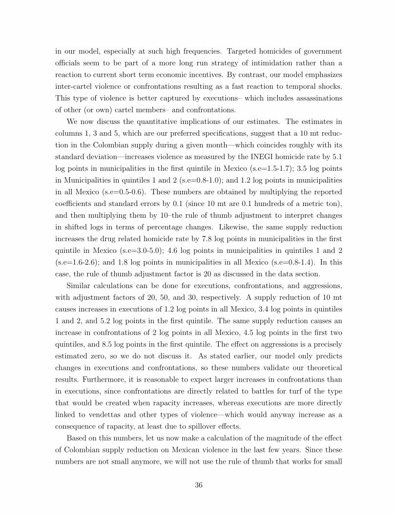
in our model, especially at such high frequencies. Targeted homicides of government
officials seem to be part of a more long run strategy of intimidation rather than a
reaction to current short term economic incentives. By contrast, our model emphasizes
inter-cartel violence or confrontations resulting as a fast reaction to temporal shocks.
This type of violence is better captured by executions– which includes assassinations
of other (or own) cartel members– and confrontations.
We now discuss the quantitative implications of our estimates. The estimates in
columns 1, 3 and 5, which are our preferred specifications, suggest that a 10 mt reduc-
tion in the Colombian supply during a given month—which coincides roughly with its
standard deviation—increases violence as measured by the INEGI homicide rate by 5.1
log points in municipalities in the first quintile in Mexico (s.e=1.5-1.7); 3.5 log points
in Municipalities in quintiles 1 and 2 (s.e=0.8-1.0); and 1.2 log points in municipalities
in all Mexico (s.e=0.5-0.6). These numbers are obtained by multiplying the reported
coefficients and standard errors by 0.1 (since 10 mt are 0.1 hundreds of a metric ton),
and then multiplying them by 10–the rule of thumb adjustment to interpret changes
in shifted logs in terms of percentage changes. Likewise, the same supply reduction
increases the drug related homicide rate by 7.8 log points in municipalities in the first
quintile in Mexico (s.e=3.0-5.0); 4.6 log points in municipalities in quintiles 1 and 2
(s.e=1.6-2.6); and 1.8 log points in municipalities in all Mexico (s.e=0.8-1.4). In this
case, the rule of thumb adjustment factor is 20 as discussed in the data section.
Similar calculations can be done for executions, confrontations, and aggressions,
with adjustment factors of 20, 50, and 30, respectively. A supply reduction of 10 mt
causes increases in executions of 1.2 log points in all Mexico, 3.4 log points in quintiles
1 and 2, and 5.2 log points in the first quintile. The same supply reduction causes an
increase in confrontations of 2 log points in all Mexico, 4.5 log points in the first two
quintiles, and 8.5 log points in the first quintile. The effect on aggressions is a precisely
estimated zero, so we do not discuss it. As stated earlier, our model only predicts
changes in executions and confrontations, so these numbers validate our theoretical
results. Furthermore, it is reasonable to expect larger increases in confrontations than
in executions, since confrontations are directly related to battles for turf of the type
that would be created when rapacity increases, whereas executions are more directly
linked to vendettas and other types of violence—which would anyway increase as a
consequence of rapacity, at least due to spillover effects.
Based on this numbers, let us now make a calculation of the magnitude of the effect
of Colombian supply reduction on Mexican violence in the last few years. Since these
numbers are not small anymore, we will not use the rule of thumb that works for small
36
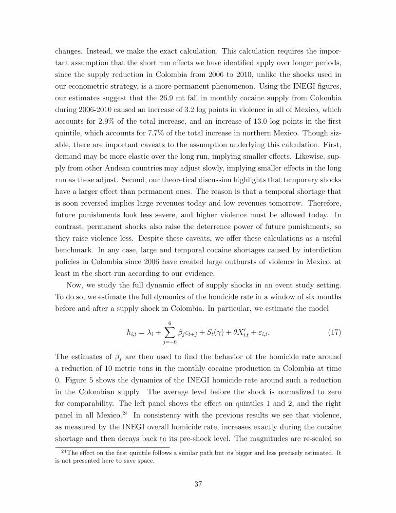
changes. Instead, we make the exact calculation. This calculation requires the impor-
tant assumption that the short run effects we have identified apply over longer periods,
since the supply reduction in Colombia from 2006 to 2010, unlike the shocks used in
our econometric strategy, is a more permanent phenomenon. Using the INEGI figures,
our estimates suggest that the 26.9 mt fall in monthly cocaine supply from Colombia
during 2006-2010 caused an increase of 3.2 log points in violence in all of Mexico, which
accounts for 2.9% of the total increase, and an increase of 13.0 log points in the first
quintile, which accounts for 7.7% of the total increase in northern Mexico. Though siz-
able, there are important caveats to the assumption underlying this calculation. First,
demand may be more elastic over the long run, implying smaller effects. Likewise, sup-
ply from other Andean countries may adjust slowly, implying smaller effects in the long
run as these adjust. Second, our theoretical discussion highlights that temporary shocks
have a larger effect than permanent ones. The reason is that a temporal shortage that
is soon reversed implies large revenues today and low revenues tomorrow. Therefore,
future punishments look less severe, and higher violence must be allowed today. In
contrast, permanent shocks also raise the deterrence power of future punishments, so
they raise violence less. Despite these caveats, we offer these calculations as a useful
benchmark. In any case, large and temporal cocaine shortages caused by interdiction
policies in Colombia since 2006 have created large outbursts of violence in Mexico, at
least in the short run according to our evidence.
Now, we study the full dynamic effect of supply shocks in an event study setting.
To do so, we estimate the full dynamics of the homicide rate in a window of six months
before and after a supply shock in Colombia. In particular, we estimate the model
hi,t = λi +6∑
j=−6
βjct+j + St(γ) + θX ′i,t + εi,t. (17)
The estimates of βj are then used to find the behavior of the homicide rate around
a reduction of 10 metric tons in the monthly cocaine production in Colombia at time
0. Figure 5 shows the dynamics of the INEGI homicide rate around such a reduction
in the Colombian supply. The average level before the shock is normalized to zero
for comparability. The left panel shows the effect on quintiles 1 and 2, and the right
panel in all Mexico.24 In consistency with the previous results we see that violence,
as measured by the INEGI overall homicide rate, increases exactly during the cocaine
shortage and then decays back to its pre-shock level. The magnitudes are re-scaled so
24The effect on the first quintile follows a similar path but its bigger and less precisely estimated. Itis not presented here to save space.
37
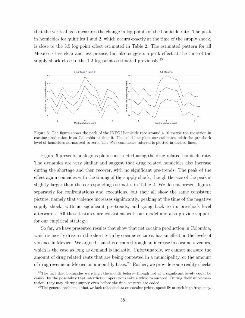
that the vertical axis measures the change in log points of the homicide rate. The peak
in homicides for quintiles 1 and 2, which occurs exactly at the time of the supply shock,
is close to the 3.5 log point effect estimated in Table 2. The estimated pattern for all
Mexico is less clear and less precise, but also suggests a peak effect at the time of the
supply shock close to the 1.2 log points estimated previously.25
−4
−2
02
46
Hom
icid
e r
ate
change in log p
oin
ts
−5 0 5Months relative to event
Quintiles 1 and 2
−2
−1
01
23
Hom
icid
e r
ate
change in log p
oin
ts
−5 0 5Months relative to event
All Mexico
Figure 5: The figure shows the path of the INEGI homicide rate around a 10 metric ton reduction incocaine production from Colombia at time 0. The solid line plots our estimates, with the pre-shocklevel of homicides normalized to zero. The 95% confidence interval is plotted in dashed lines.
Figure 6 presents analogous plots constructed using the drug related homicide rate.
The dynamics are very similar and suggest that drug related homicides also increase
during the shortage and then recover, with no significant pre-trends. The peak of the
effect again coincides with the timing of the supply shock, though the size of the peak is
slightly larger than the corresponding estimates in Table 2. We do not present figures
separately for confrontations and executions, but they all show the same consistent
picture, namely that violence increases significantly, peaking at the time of the negative
supply shock, with no significant pre-trends, and going back to its pre-shock level
afterwards. All these features are consistent with our model and also provide support
for our empirical strategy.
So far, we have presented results that show that net cocaine production in Colombia,
which is mostly driven in the short term by cocaine seizures, has an effect on the levels of
violence in Mexico. We argued that this occurs through an increase in cocaine revenues,
which is the case as long as demand is inelastic. Unfortunately, we cannot measure the
amount of drug related rents that are being contested in a municipality, or the amount
of drug revenue in Mexico on a monthly basis.26 Rather, we provide some reality checks
25The fact that homicides were high the month before– though not at a significant level– could becaused by the possibility that interdiction operations take a while to succeed. During their implemen-tation, they may disrupt supply even before the final seizures are coded.
26The general problem is that we lack reliable data on cocaine prices, specially at such high frequency.
38
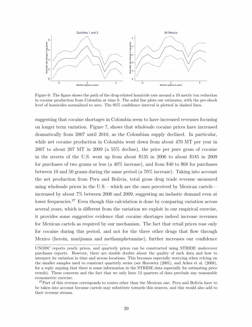
−10
−5
05
10
Hom
icid
e r
ate
change in log p
oin
ts
−5 0 5Months relative to event
Quintiles 1 and 2
−6
−4
−2
02
4H
om
icid
e r
ate
change in log p
oin
ts
−5 0 5Months relative to event
All Mexico
Figure 6: The figure shows the path of the drug-related homicide rate around a 10 metric ton reductionin cocaine production from Colombia at time 0. The solid line plots our estimates, with the pre-shocklevel of homicides normalized to zero. The 95% confidence interval is plotted in dashed lines.
suggesting that cocaine shortages in Colombia seem to have increased revenues focusing
on longer term variation. Figure 7, shows that wholesale cocaine prices have increased
dramatically from 2007 until 2010, as the Colombian supply declined. In particular,
while net cocaine production in Colombia went down from about 470 MT per year in
2007 to about 207 MT in 2009 (a 55% decline), the price per pure gram of cocaine
in the streets of the U.S. went up from about $135 in 2006 to about $185 in 2009
for purchases of two grams or less (a 40% increase), and from $40 to $68 for purchases
between 10 and 50 grams during the same period (a 70% increase). Taking into account
the net production from Peru and Bolivia, total gross drug trade revenue measured
using wholesale prices in the U.S.—which are the ones perceived by Mexican cartels—
increased by about 7% between 2006 and 2009, suggesting an inelastic demand even at
lower frequencies.27 Even though this calculation is done by comparing variation across
several years, which is different from the variation we exploit in our empirical exercise,
it provides some suggestive evidence that cocaine shortages indeed increase revenues
for Mexican cartels as required by our mechanism. The fact that retail prices rose only
for cocaine during this period, and not for the three other drugs that flow through
Mexico (heroin, marijuana and methamphetamine), further increases our confidence
UNODC reports yearly prices, and quarterly prices can be constructed using STRIDE undercoverpurchases reports. However, there are sizable doubts about the quality of such data and how tointerpret its variation in time and across locations. This becomes especially worrying when relying onthe smaller samples used to construct quarterly series (see Horowitz (2001), and Arkes et al. (2008),for a reply arguing that there is some information in the STRIDE data especially for estimating pricetrends). These concerns and the fact that we only have 12 quarters of data preclude any reasonableeconometric exercise.
27Part of this revenue corresponds to routes other than the Mexican one. Peru and Bolivia have tobe taken into account because cartels may substitute towards this sources, and this would also add totheir revenue stream.
39
that increases in Colombian cocaine seizures had an effect on violence in Mexico through
the increase in cocaine prices and rents associated to the cocaine market.
100
120
140
160
180
200
Reta
il price p
er
gra
m
050
100
150
Metr
ic tons
2007m1 2008m1 2009m1 2010m1 2011m1Month
Quarterly production Cocaine price
Figure 7: The figure shows the quarterly cocaine production in Colombia net of seizures (left axis) andthe quarterly cocaine prices reported by STRIDE (right axis). Prices are per dollar for pure gram inwholesale transactions, while production is in hundred metric tons per quarter.
6.2 Heterogeneity by importance for trafficking
In this section we investigate the prediction in proposition 1 regarding the importance
of a municipality for trafficking. Casual observation suggests that municipalities that
are closer to entry points in the U.S.-Mexico border will be more important for cocaine
trafficking. Unlike heroin or cannabis, cocaine is not produced in Mexico, so the strate-
gic position of a municipality in terms of trafficking determines its importance. Figure
8 presents maps of Mexico showing that drug trafficking has a clear spatial allocation,
with drug related homicides, cocaine seizures by Mexican authorities and cartel pres-
ence concentrated on the northeast region, close to the Gulf of Mexico and next to the
U.S. border, the northwest of the country, and the Pacific region southwest of Mexico
City, especially in the states of Michoacan and Guerrero. These maps thus show that,
in broad terms, the regions where drug trafficking and violence are more intense tend to
be located either close to U.S. entry points (because of their importance for smuggling)
or near the ports in the southwest of Mexico, which are important points of entry of
cocaine from Colombia. We focus on the distance to the U.S. as our main measure
of importance for trafficking because drug related activities in the Pacific seem to be
unique to two states (Michoacan and Guerrero), while they are more widespread in
the north. Distance to the U.S. entry points is therefore our preferred proxy for the
40
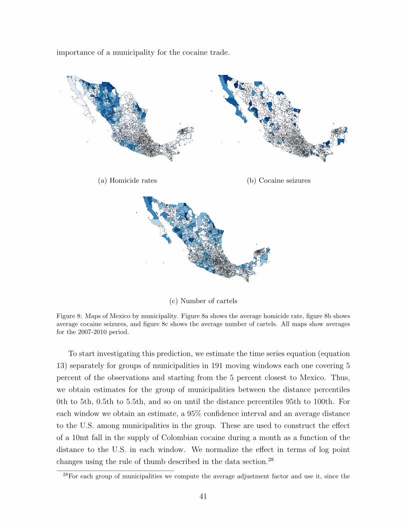
importance of a municipality for the cocaine trade.
(a) Homicide rates (b) Cocaine seizures
(c) Number of cartels
Figure 8: Maps of Mexico by municipality. Figure 8a shows the average homicide rate, figure 8b showsaverage cocaine seizures, and figure 8c shows the average number of cartels. All maps show averagesfor the 2007-2010 period.
To start investigating this prediction, we estimate the time series equation (equation
13) separately for groups of municipalities in 191 moving windows each one covering 5
percent of the observations and starting from the 5 percent closest to Mexico. Thus,
we obtain estimates for the group of municipalities between the distance percentiles
0th to 5th, 0.5th to 5.5th, and so on until the distance percentiles 95th to 100th. For
each window we obtain an estimate, a 95% confidence interval and an average distance
to the U.S. among municipalities in the group. These are used to construct the effect
of a 10mt fall in the supply of Colombian cocaine during a month as a function of the
distance to the U.S. in each window. We normalize the effect in terms of log point
changes using the rule of thumb described in the data section.28
28For each group of municipalities we compute the average adjustment factor and use it, since the
41
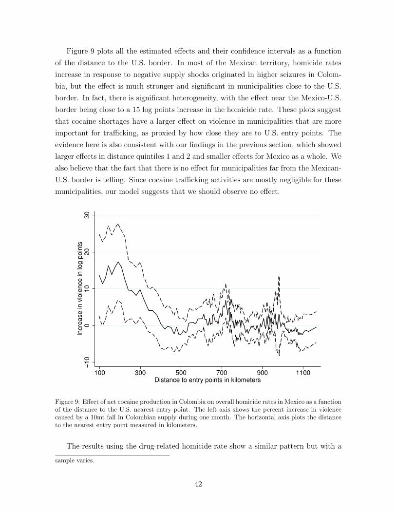
Figure 9 plots all the estimated effects and their confidence intervals as a function
of the distance to the U.S. border. In most of the Mexican territory, homicide rates
increase in response to negative supply shocks originated in higher seizures in Colom-
bia, but the effect is much stronger and significant in municipalities close to the U.S.
border. In fact, there is significant heterogeneity, with the effect near the Mexico-U.S.
border being close to a 15 log points increase in the homicide rate. These plots suggest
that cocaine shortages have a larger effect on violence in municipalities that are more
important for trafficking, as proxied by how close they are to U.S. entry points. The
evidence here is also consistent with our findings in the previous section, which showed
larger effects in distance quintiles 1 and 2 and smaller effects for Mexico as a whole. We
also believe that the fact that there is no effect for municipalities far from the Mexican-
U.S. border is telling. Since cocaine trafficking activities are mostly negligible for these
municipalities, our model suggests that we should observe no effect.
−10
010
20
30
Incre
ase in v
iole
nce in log p
oin
ts
100 300 500 700 900 1100Distance to entry points in kilometers
Figure 9: Effect of net cocaine production in Colombia on overall homicide rates in Mexico as a functionof the distance to the U.S. nearest entry point. The left axis shows the percent increase in violencecaused by a 10mt fall in Colombian supply during one month. The horizontal axis plots the distanceto the nearest entry point measured in kilometers.
The results using the drug-related homicide rate show a similar pattern but with a
sample varies.
42
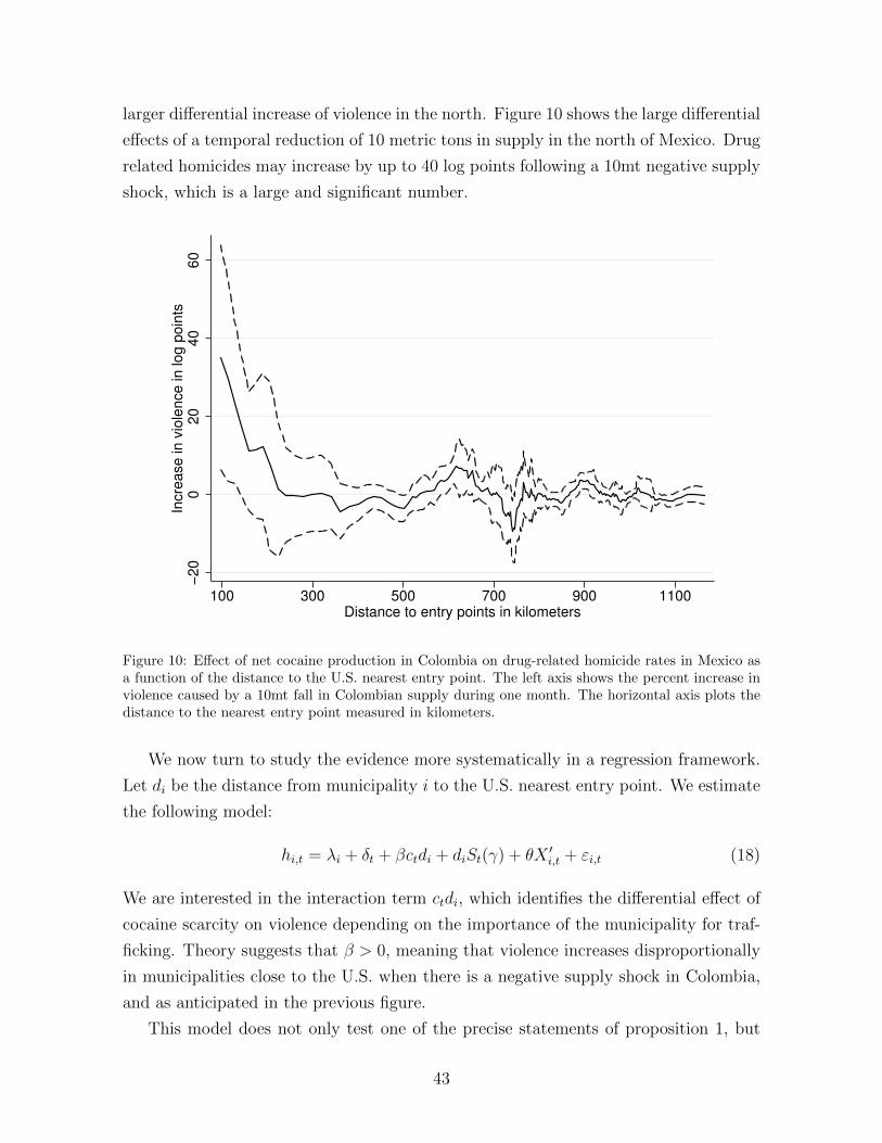
larger differential increase of violence in the north. Figure 10 shows the large differential
effects of a temporal reduction of 10 metric tons in supply in the north of Mexico. Drug
related homicides may increase by up to 40 log points following a 10mt negative supply
shock, which is a large and significant number.−
20
020
40
60
Incre
ase in v
iole
nce in log p
oin
ts
100 300 500 700 900 1100Distance to entry points in kilometers
Figure 10: Effect of net cocaine production in Colombia on drug-related homicide rates in Mexico asa function of the distance to the U.S. nearest entry point. The left axis shows the percent increase inviolence caused by a 10mt fall in Colombian supply during one month. The horizontal axis plots thedistance to the nearest entry point measured in kilometers.
We now turn to study the evidence more systematically in a regression framework.
Let di be the distance from municipality i to the U.S. nearest entry point. We estimate
the following model:
hi,t = λi + δt + βctdi + diSt(γ) + θX ′i,t + εi,t (18)
We are interested in the interaction term ctdi, which identifies the differential effect of
cocaine scarcity on violence depending on the importance of the municipality for traf-
ficking. Theory suggests that β > 0, meaning that violence increases disproportionally
in municipalities close to the U.S. when there is a negative supply shock in Colombia,
and as anticipated in the previous figure.
This model does not only test one of the precise statements of proposition 1, but
43
also provides another broad test of our mechanism. In particular, the effect of scarcity
should be stronger in places where the cocaine trade and trafficking are more intense.
Thus, finding that shortages increase violence in these places relative to the average
municipality provides additional evidence for our mechanism, which exploits both the
time series and the cross sectional dimensions of our data. In other words, we regard
this exercise as providing within municipality evidence of our mechanism, exploiting
the fact that the importance of a municipality for trafficking varies cross sectionally. In
contrast, the previous section focused on the pure time series evidence of our mecha-
nism. We believe that our estimates of β in equation 18 can be interpreted as causal
because distance is exogenous once we condition on fixed effects and control for any
secular trends in homicides that vary by distance—using the controls diSt(γ). Thus,
our estimates do not exploit the fact that the north was becoming more violent over
time, but the fact that during months with negative supply shocks in Colombia, vi-
olence in municipalities located closer to entry points deviates differentially from its
trend behavior. The coefficient β captures this differential short run response.
Table 3 presents our estimation results for different dependent variables. The top
panel presents results using the transformed INEGI homicide rate as the dependent
variable; while the other panels present results for the drug related homicide rate and
its components. Columns 1 to 4 estimate equation 18 for all Mexican municipalities;
while columns 5 to 8 restrict the sample to municipalities in distance quintiles 1 and
2. As before, we restrict ourselves to the closest quintiles to focus on the north of
Mexico, where we believe drug trafficking and our model has more predictive power
for violence, and because municipalities close to U.S. entry points can be expected to
be more similar to each other, making our comparisons more accurate (there are many
reasons to believe that municipalities in the north of Mexico are systematically different
from municipalities in the south). All municipalities in this group have experienced the
consequences of drug trafficking more severely than the rest of the country, so focusing
on these municipalities provides a cleaner experiment. We only report estimates for the
effect of the interaction term, since the main effect of shortages is not identified once
we include month fixed effects.
Columns 1 and 5 present results controlling only for a differential cubic trend by
distance to the U.S. (that is, when St(γ) includes a cubic polynomial and year dum-
mies). The results vary little if we use higher order polynomials, so we stick to a cubic
polynomial throughout.29 The results using the INEGI homicide rate suggest that a
29Table 8 in the appendix shows that the estimates do not vary significantly for polynomials ofdegree two or higher.
44
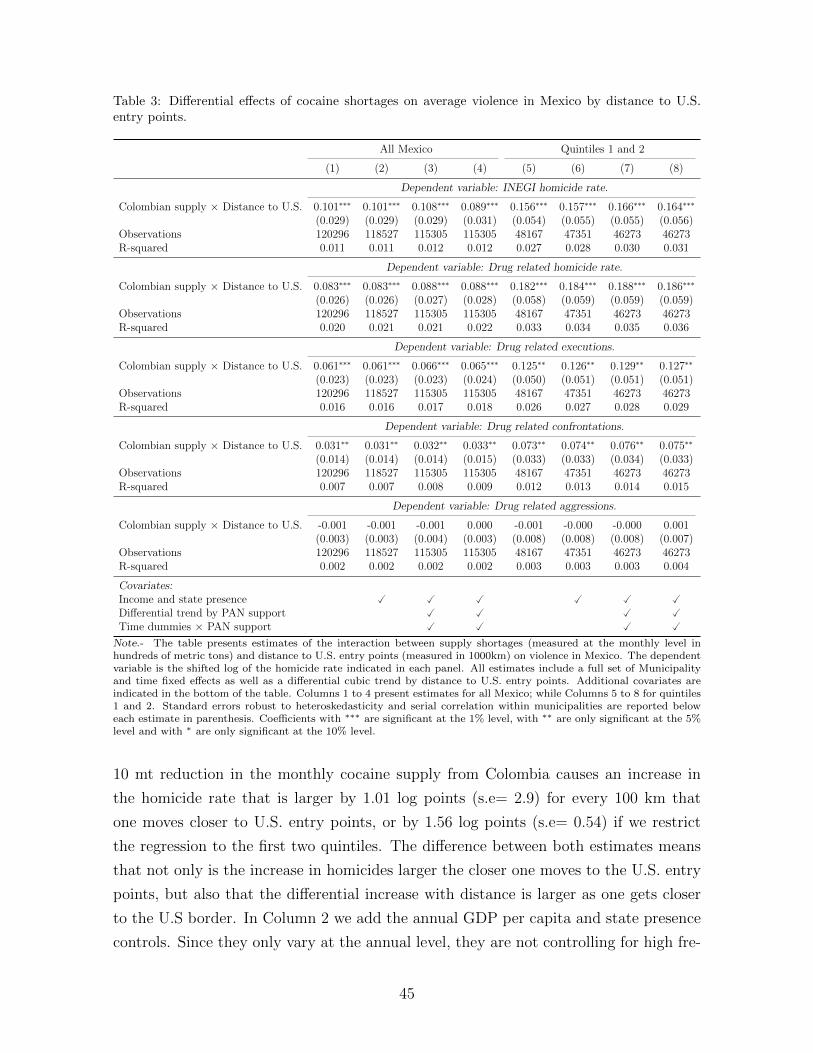
Table 3: Differential effects of cocaine shortages on average violence in Mexico by distance to U.S.entry points.
All Mexico Quintiles 1 and 2
(1) (2) (3) (4) (5) (6) (7) (8)
Dependent variable: INEGI homicide rate.
Colombian supply × Distance to U.S. 0.101∗∗∗ 0.101∗∗∗ 0.108∗∗∗ 0.089∗∗∗ 0.156∗∗∗ 0.157∗∗∗ 0.166∗∗∗ 0.164∗∗∗
(0.029) (0.029) (0.029) (0.031) (0.054) (0.055) (0.055) (0.056)Observations 120296 118527 115305 115305 48167 47351 46273 46273R-squared 0.011 0.011 0.012 0.012 0.027 0.028 0.030 0.031
Dependent variable: Drug related homicide rate.
Colombian supply × Distance to U.S. 0.083∗∗∗ 0.083∗∗∗ 0.088∗∗∗ 0.088∗∗∗ 0.182∗∗∗ 0.184∗∗∗ 0.188∗∗∗ 0.186∗∗∗
(0.026) (0.026) (0.027) (0.028) (0.058) (0.059) (0.059) (0.059)Observations 120296 118527 115305 115305 48167 47351 46273 46273R-squared 0.020 0.021 0.021 0.022 0.033 0.034 0.035 0.036
Dependent variable: Drug related executions.
Colombian supply × Distance to U.S. 0.061∗∗∗ 0.061∗∗∗ 0.066∗∗∗ 0.065∗∗∗ 0.125∗∗ 0.126∗∗ 0.129∗∗ 0.127∗∗
(0.023) (0.023) (0.023) (0.024) (0.050) (0.051) (0.051) (0.051)Observations 120296 118527 115305 115305 48167 47351 46273 46273R-squared 0.016 0.016 0.017 0.018 0.026 0.027 0.028 0.029
Dependent variable: Drug related confrontations.
Colombian supply × Distance to U.S. 0.031∗∗ 0.031∗∗ 0.032∗∗ 0.033∗∗ 0.073∗∗ 0.074∗∗ 0.076∗∗ 0.075∗∗
(0.014) (0.014) (0.014) (0.015) (0.033) (0.033) (0.034) (0.033)Observations 120296 118527 115305 115305 48167 47351 46273 46273R-squared 0.007 0.007 0.008 0.009 0.012 0.013 0.014 0.015
Dependent variable: Drug related aggressions.
Colombian supply × Distance to U.S. -0.001 -0.001 -0.001 0.000 -0.001 -0.000 -0.000 0.001(0.003) (0.003) (0.004) (0.003) (0.008) (0.008) (0.008) (0.007)
Observations 120296 118527 115305 115305 48167 47351 46273 46273R-squared 0.002 0.002 0.002 0.002 0.003 0.003 0.003 0.004
Covariates:Income and state presence � � � � � �Differential trend by PAN support � � � �Time dummies × PAN support � � � �
Note.- The table presents estimates of the interaction between supply shortages (measured at the monthly level inhundreds of metric tons) and distance to U.S. entry points (measured in 1000km) on violence in Mexico. The dependentvariable is the shifted log of the homicide rate indicated in each panel. All estimates include a full set of Municipalityand time fixed effects as well as a differential cubic trend by distance to U.S. entry points. Additional covariates areindicated in the bottom of the table. Columns 1 to 4 present estimates for all Mexico; while Columns 5 to 8 for quintiles1 and 2. Standard errors robust to heteroskedasticity and serial correlation within municipalities are reported beloweach estimate in parenthesis. Coefficients with ∗∗∗ are significant at the 1% level, with ∗∗ are only significant at the 5%level and with ∗ are only significant at the 10% level.
10 mt reduction in the monthly cocaine supply from Colombia causes an increase in
the homicide rate that is larger by 1.01 log points (s.e= 2.9) for every 100 km that
one moves closer to U.S. entry points, or by 1.56 log points (s.e= 0.54) if we restrict
the regression to the first two quintiles. The difference between both estimates means
that not only is the increase in homicides larger the closer one moves to the U.S. entry
points, but also that the differential increase with distance is larger as one gets closer
to the U.S border. In Column 2 we add the annual GDP per capita and state presence
controls. Since they only vary at the annual level, they are not controlling for high fre-
45
quency socio-economic phenomena, but for differential time trends (or lower frequency
variation) in municipalities with different characteristics that could be related to their
distance to the U.S. entry points. Our estimates vary little, suggesting that we are not
capturing differential trends depending on income or state presence. We do not think
that adding these controls creates a significant bad control problem. Even though in-
come and state presence could be endogenous, their annual variation is less so, and
simply helps us control for different longer term trends. In any case, all of our results
hold without these controls as well.
In Columns 3, 4, 7, and 8 we control flexibly for enforcement policies that were
being implemented during our period of analysis. As mentioned above, since 2006, the
Calderon administration started an aggressive campaign of cracking down on cartels.
As shown by Dell (2013) this was especially the case in municipalities with PAN mayors,
where there was support for these policies and cooperation by local authorities. Instead
of controlling for the presence of a PAN mayor, which we see as a bad control due to
its potential endogeneity, we control for differential cubic trends by historical PAN
support (vote share from 1990 to 2000) in Columns 3 and 7, or a full set of time
dummies interacted with historical PAN support in Columns 4 and 8.30 The intuition
is that places in which the PAN held more political power, as captured by its historical
vote share, are more likely to have PAN mayors or directly offer cooperation for Federal
PAN policies. Thus, the models in these columns fully control for differential patterns of
violence in more pro-PAN municipalities. Our estimates do not change much, suggesting
that we are not capturing a correlation in time between our supply shocks and their
differential effect on the north, and PAN policies that were intensified during our period
of analysis.
The second panel presents results using the drug related homicide rate as the de-
pendent variable. The structure is the same as the top panel. The point estimates and
their significance are similar to the ones discussed above, but the implied magnitudes
are different since we must use a different factor of adjustment. In particular, the results
using the drug-related homicide rate suggest that a reduction of 10 metric tons in the
monthly cocaine production in Colombia increases drug related homicides by 1.66 log
points more (s.e=0.52) for every 100km that one moves closer to a U.S. entry point.
The gradient becomes even steeper in the north: In quintiles 1 and 2, every 100km
that one moves closer to the U.S. imply that the same supply shock increases violence
30On some results not reported here, we obtained very similar results using the presence of a PANmayor as a control. Though endogenous, this shows that our estimates are not driven by the electionof PAN mayors during the Calderon administration.
46
by 3.64 log points (s.e=1.16). These estimates suggest that for drug-related homicides,
the differential effect on the north is even stronger relative to southern municipalities
with little or no involvement in cocaine trafficking.
The bottom panels explore the categories into which drug related homicides are
separated. Our findings agree with the time series results of table 2: The interaction
coefficients for both executions and confrontations are positive and significant, whereas
the coefficients for aggressions are small and not significant. The effect for confronta-
tions is larger than the effect for executions (remember that the adjustment factor for
confrontations is 50, whereas the adjustment factor for executions is 20). These results
further support our model, which predicts differential increases in violence between car-
tels (such as executions and confrontations) in response to scarcity shocks in the north
of Mexico, but it is silent about effects on violence between government authorities
and cartels of the type captured by aggressions. Among violence between cartels, the
type of violence that should be most strongly affected are battles for turf caused by
rapacity, and homicides due to this type of battles are classified as confrontations. Our
econometric results show that this type of violence increases more than the others, and
does so differentially in the north of Mexico, following a supply contraction.
Our results show that the scarcity created by larger and more frequent negative
supply shocks in Colombia since 2006 has contributed to the increase in violence in the
north relative to the rest of the country. To get an idea of these magnitudes, consider
Tijuana, which is on an entry point, and Puebla, which is in the mean distance (about
760 km away from the U.S. border). If cocaine supply from Colombia falls by 10 mt
in a given month, our estimates suggest that the homicide rate increases by 11.86 log
points more in Tijuana than in Puebla (in this calculation we used the coefficient for
quintiles 1 and 2, since cities at the mean distance and at the U.S. border lie in this
sample). Drug related homicides increase by 32 log points more in Tijuana than in
Puebla. Suppose that the effect of a permanent supply fall is the same as a short
run shock, with all the caveats that this assumption requires and that were already
discussed. Between 2006-2010, the Colombian monthly supply of cocaine fell by 26.9
mt (from 43.5 mt to 16.6 mt). Scarcity created by Colombian policies could explain up
to 20% of the differential increase in homicide rates between Tijuana and Puebla from
2006 to 2010. More generally, with the assumption above, our estimates imply that the
scarcity created by Colombian policies caused a 32 log point increase in violence near
U.S. border crossings relative to the mean distance. Thus, the large drop in Colombian
supply could account for up to 25% of the 128 log point differential increase of violence
in the north of Mexico during our period of study (in this sense, Tijuana and Puebla are
47
similar to the sample averages). The contribution of scarcity appears to be even larger
if we use the semi-parametrical estimates plotted in figures 9 and 10. In particular, our
channel may explain up to 21.2% and 46% of the observed increase in overall and drug
related homicides, respectively, in the 5 percent closest municipalities to the U.S., while
it has no significant explanatory power in the south.
6.3 Role of cartels: It takes two to tango.
As suggested by our theoretical model, the presence of cartels in a municipality should
also be important in determining whether negative supply shocks in wholesale cocaine
markets breed violence, as municipalities without cartels should not see their levels of
drug related violence increased as a result of supply tightenings in wholesale cocaine
markets. Furthermore, the number of cartels should also be important because different
theories point out that territories that are disputed between various factions should
display higher levels of violence, while territories under the full control of a single
faction should exhibit low levels of violence (see Grossman (2001) and Kalyvas (2006)
for a similar argument). In fact, many critics of the Calderon administration have
pointed out that it fragmented cohesive cartels, leading to more violence (see Guerrero
(2010, 2011a) and Merino (2011)). In our model, whenever a cartel fully controls a
municipality, its property rights over the revenue stream generated in that municipality
are well established. In contrast, as the number of cartels increases, the rapacity effect
becomes active: To secure rents, cartels must fight each other. They would like to
divide the pie and not use violence, but every cartel would be tempted to deviate and
use violence to appropriate a larger share of the pie. This is the classic Olson paradox
in the context of inter-cartel conflict.
In order to test this hypothesis, we use the data produced by Coscia and Rıos
(2012) on the presence of Mexican cartels in each municipality. Although this data
is only available on a yearly basis, which means that we cannot measure how high
frequency changes in the number of cartels affect violence, it allows us to measure the
differential effects of supply shocks in cocaine markets depending on the number of
cartels present in each municipality. We start by estimating time series results for the
subsample of municipalities with no cartels, one cartel, two cartels (rival or non-rival)
and two rival cartels at the time of the shock. We present our results using event study
figures showing the change in the homicide rate in log points around a temporal fall of
10 metric tons at month zero (like figures 5 and 6), but the regression results are very
similar. We focus on the overall homicide rate and in municipalities in quintiles 1 and
48
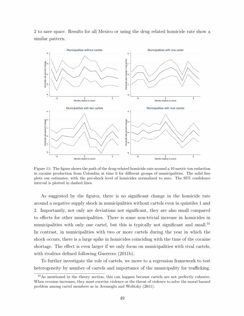
2 to save space. Results for all Mexico or using the drug related homicide rate show a
similar pattern.
−.4
−.2
0.2
.4H
om
icid
e r
ate
perc
ent change
−5 0 5Months relative to event
Municipalities without cartels
−2
−1
01
2H
om
icid
e r
ate
change in log p
oin
ts
−5 0 5Months relative to event
Municipalities with one cartel−
2−
10
12
3H
om
icid
e r
ate
perc
ent change
−5 0 5Months relative to event
Municipalities with two cartels
−4
−2
02
4H
om
icid
e r
ate
perc
ent change
−5 0 5Months relative to event
Municipalities with rival cartels
Figure 11: The figure shows the path of the drug-related homicide rate around a 10 metric ton reductionin cocaine production from Colombia at time 0 for different groups of municipalities. The solid lineplots our estimates, with the pre-shock level of homicides normalized to zero. The 95% confidenceinterval is plotted in dashed lines.
As suggested by the figures, there is no significant change in the homicide rate
around a negative supply shock in municipalities without cartels even in quintiles 1 and
2. Importantly, not only are deviations not significant, they are also small compared
to effects for other municipalities. There is some non-trivial increase in homicides in
municipalities with only one cartel, but this is typically not significant and small.31
In contrast, in municipalities with two or more cartels during the year in which the
shock occurs, there is a large spike in homicides coinciding with the time of the cocaine
shortage. The effect is even larger if we only focus on municipalities with rival cartels,
with rivalries defined following Guerrero (2011b).
To further investigate the role of cartels, we move to a regression framework to test
heterogeneity by number of cartels and importance of the municipality for trafficking.
31As mentioned in the theory section, this can happen because cartels are not perfectly cohesive.When revenue increases, they must exercise violence or the threat of violence to solve the moral hazardproblem among cartel members as in Acemoglu and Wolitzky (2011).
49
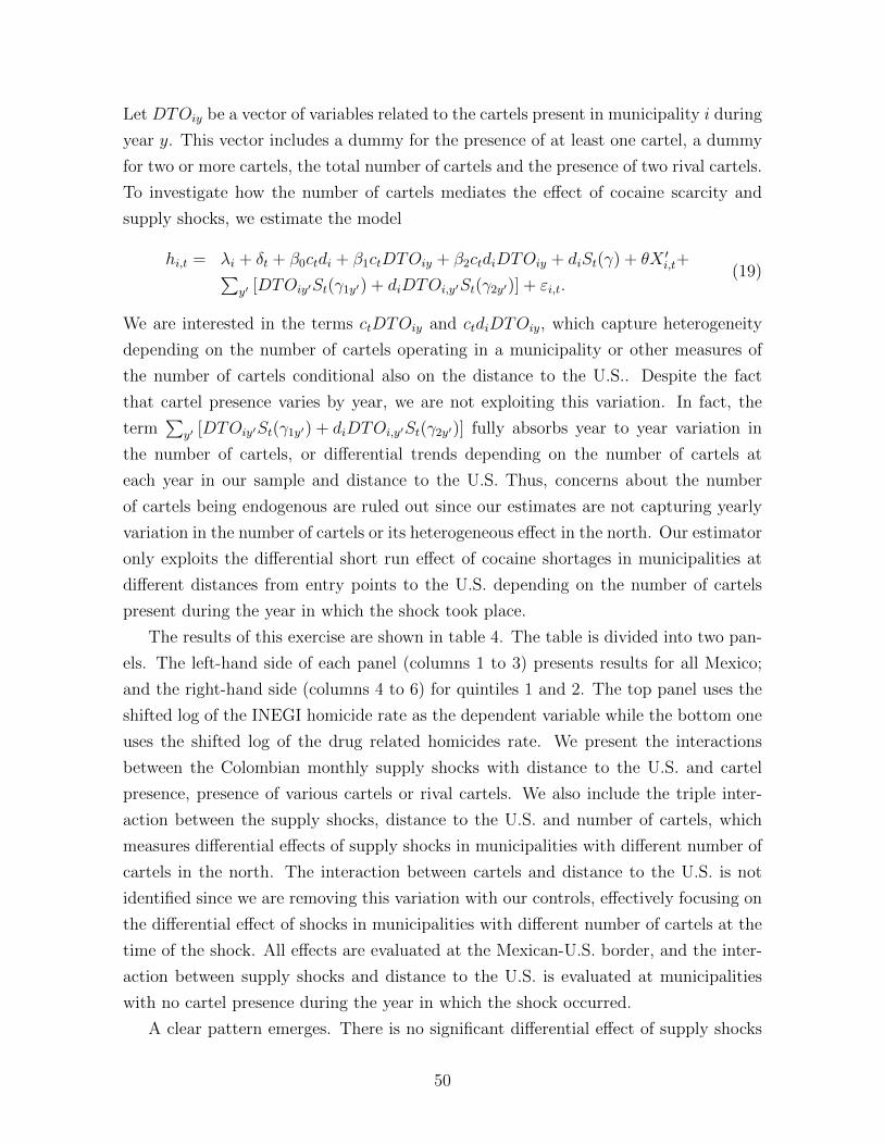
Let DTOiy be a vector of variables related to the cartels present in municipality i during
year y. This vector includes a dummy for the presence of at least one cartel, a dummy
for two or more cartels, the total number of cartels and the presence of two rival cartels.
To investigate how the number of cartels mediates the effect of cocaine scarcity and
supply shocks, we estimate the model
hi,t = λi + δt + β0ctdi + β1ctDTOiy + β2ctdiDTOiy + diSt(γ) + θX ′i,t+∑y′ [DTOiy′St(γ1y′) + diDTOi,y′St(γ2y′)] + εi,t.
(19)
We are interested in the terms ctDTOiy and ctdiDTOiy, which capture heterogeneity
depending on the number of cartels operating in a municipality or other measures of
the number of cartels conditional also on the distance to the U.S.. Despite the fact
that cartel presence varies by year, we are not exploiting this variation. In fact, the
term∑
y′ [DTOiy′St(γ1y′) + diDTOi,y′St(γ2y′)] fully absorbs year to year variation in
the number of cartels, or differential trends depending on the number of cartels at
each year in our sample and distance to the U.S. Thus, concerns about the number
of cartels being endogenous are ruled out since our estimates are not capturing yearly
variation in the number of cartels or its heterogeneous effect in the north. Our estimator
only exploits the differential short run effect of cocaine shortages in municipalities at
different distances from entry points to the U.S. depending on the number of cartels
present during the year in which the shock took place.
The results of this exercise are shown in table 4. The table is divided into two pan-
els. The left-hand side of each panel (columns 1 to 3) presents results for all Mexico;
and the right-hand side (columns 4 to 6) for quintiles 1 and 2. The top panel uses the
shifted log of the INEGI homicide rate as the dependent variable while the bottom one
uses the shifted log of the drug related homicides rate. We present the interactions
between the Colombian monthly supply shocks with distance to the U.S. and cartel
presence, presence of various cartels or rival cartels. We also include the triple inter-
action between the supply shocks, distance to the U.S. and number of cartels, which
measures differential effects of supply shocks in municipalities with different number of
cartels in the north. The interaction between cartels and distance to the U.S. is not
identified since we are removing this variation with our controls, effectively focusing on
the differential effect of shocks in municipalities with different number of cartels at the
time of the shock. All effects are evaluated at the Mexican-U.S. border, and the inter-
action between supply shocks and distance to the U.S. is evaluated at municipalities
with no cartel presence during the year in which the shock occurred.
A clear pattern emerges. There is no significant differential effect of supply shocks
50
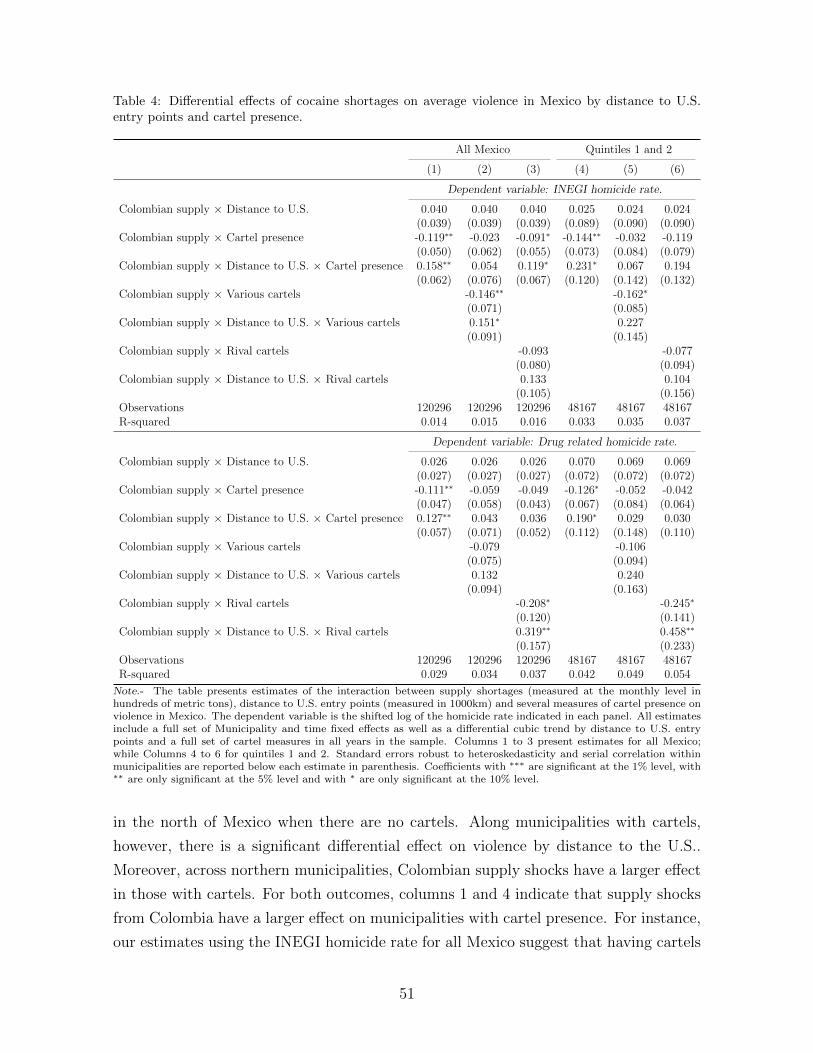
Table 4: Differential effects of cocaine shortages on average violence in Mexico by distance to U.S.entry points and cartel presence.
All Mexico Quintiles 1 and 2
(1) (2) (3) (4) (5) (6)
Dependent variable: INEGI homicide rate.
Colombian supply × Distance to U.S. 0.040 0.040 0.040 0.025 0.024 0.024(0.039) (0.039) (0.039) (0.089) (0.090) (0.090)
Colombian supply × Cartel presence -0.119∗∗ -0.023 -0.091∗ -0.144∗∗ -0.032 -0.119(0.050) (0.062) (0.055) (0.073) (0.084) (0.079)
Colombian supply × Distance to U.S. × Cartel presence 0.158∗∗ 0.054 0.119∗ 0.231∗ 0.067 0.194(0.062) (0.076) (0.067) (0.120) (0.142) (0.132)
Colombian supply × Various cartels -0.146∗∗ -0.162∗
(0.071) (0.085)Colombian supply × Distance to U.S. × Various cartels 0.151∗ 0.227
(0.091) (0.145)Colombian supply × Rival cartels -0.093 -0.077
(0.080) (0.094)Colombian supply × Distance to U.S. × Rival cartels 0.133 0.104
(0.105) (0.156)Observations 120296 120296 120296 48167 48167 48167R-squared 0.014 0.015 0.016 0.033 0.035 0.037
Dependent variable: Drug related homicide rate.
Colombian supply × Distance to U.S. 0.026 0.026 0.026 0.070 0.069 0.069(0.027) (0.027) (0.027) (0.072) (0.072) (0.072)
Colombian supply × Cartel presence -0.111∗∗ -0.059 -0.049 -0.126∗ -0.052 -0.042(0.047) (0.058) (0.043) (0.067) (0.084) (0.064)
Colombian supply × Distance to U.S. × Cartel presence 0.127∗∗ 0.043 0.036 0.190∗ 0.029 0.030(0.057) (0.071) (0.052) (0.112) (0.148) (0.110)
Colombian supply × Various cartels -0.079 -0.106(0.075) (0.094)
Colombian supply × Distance to U.S. × Various cartels 0.132 0.240(0.094) (0.163)
Colombian supply × Rival cartels -0.208∗ -0.245∗
(0.120) (0.141)Colombian supply × Distance to U.S. × Rival cartels 0.319∗∗ 0.458∗∗
(0.157) (0.233)Observations 120296 120296 120296 48167 48167 48167R-squared 0.029 0.034 0.037 0.042 0.049 0.054
Note.- The table presents estimates of the interaction between supply shortages (measured at the monthly level inhundreds of metric tons), distance to U.S. entry points (measured in 1000km) and several measures of cartel presence onviolence in Mexico. The dependent variable is the shifted log of the homicide rate indicated in each panel. All estimatesinclude a full set of Municipality and time fixed effects as well as a differential cubic trend by distance to U.S. entrypoints and a full set of cartel measures in all years in the sample. Columns 1 to 3 present estimates for all Mexico;while Columns 4 to 6 for quintiles 1 and 2. Standard errors robust to heteroskedasticity and serial correlation withinmunicipalities are reported below each estimate in parenthesis. Coefficients with ∗∗∗ are significant at the 1% level, with∗∗ are only significant at the 5% level and with ∗ are only significant at the 10% level.
in the north of Mexico when there are no cartels. Along municipalities with cartels,
however, there is a significant differential effect on violence by distance to the U.S..
Moreover, across northern municipalities, Colombian supply shocks have a larger effect
in those with cartels. For both outcomes, columns 1 and 4 indicate that supply shocks
from Colombia have a larger effect on municipalities with cartel presence. For instance,
our estimates using the INEGI homicide rate for all Mexico suggest that having cartels
51
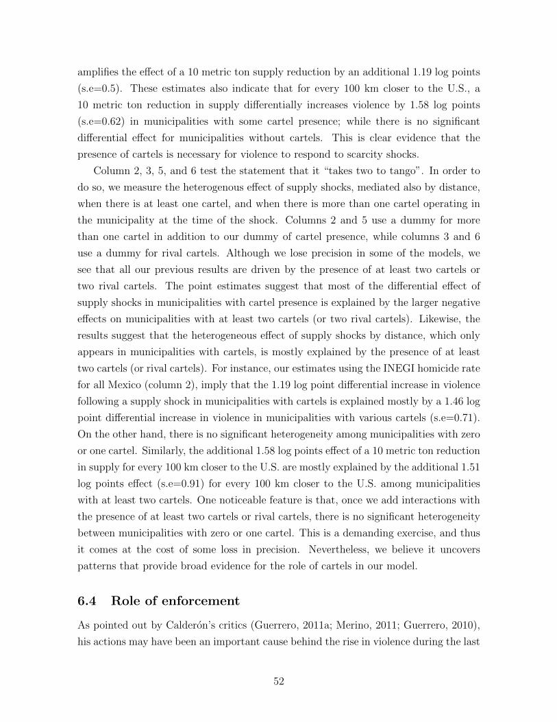
amplifies the effect of a 10 metric ton supply reduction by an additional 1.19 log points
(s.e=0.5). These estimates also indicate that for every 100 km closer to the U.S., a
10 metric ton reduction in supply differentially increases violence by 1.58 log points
(s.e=0.62) in municipalities with some cartel presence; while there is no significant
differential effect for municipalities without cartels. This is clear evidence that the
presence of cartels is necessary for violence to respond to scarcity shocks.
Column 2, 3, 5, and 6 test the statement that it “takes two to tango”. In order to
do so, we measure the heterogenous effect of supply shocks, mediated also by distance,
when there is at least one cartel, and when there is more than one cartel operating in
the municipality at the time of the shock. Columns 2 and 5 use a dummy for more
than one cartel in addition to our dummy of cartel presence, while columns 3 and 6
use a dummy for rival cartels. Although we lose precision in some of the models, we
see that all our previous results are driven by the presence of at least two cartels or
two rival cartels. The point estimates suggest that most of the differential effect of
supply shocks in municipalities with cartel presence is explained by the larger negative
effects on municipalities with at least two cartels (or two rival cartels). Likewise, the
results suggest that the heterogeneous effect of supply shocks by distance, which only
appears in municipalities with cartels, is mostly explained by the presence of at least
two cartels (or rival cartels). For instance, our estimates using the INEGI homicide rate
for all Mexico (column 2), imply that the 1.19 log point differential increase in violence
following a supply shock in municipalities with cartels is explained mostly by a 1.46 log
point differential increase in violence in municipalities with various cartels (s.e=0.71).
On the other hand, there is no significant heterogeneity among municipalities with zero
or one cartel. Similarly, the additional 1.58 log points effect of a 10 metric ton reduction
in supply for every 100 km closer to the U.S. are mostly explained by the additional 1.51
log points effect (s.e=0.91) for every 100 km closer to the U.S. among municipalities
with at least two cartels. One noticeable feature is that, once we add interactions with
the presence of at least two cartels or rival cartels, there is no significant heterogeneity
between municipalities with zero or one cartel. This is a demanding exercise, and thus
it comes at the cost of some loss in precision. Nevertheless, we believe it uncovers
patterns that provide broad evidence for the role of cartels in our model.
6.4 Role of enforcement
As pointed out by Calderon’s critics (Guerrero, 2011a; Merino, 2011; Guerrero, 2010),
his actions may have been an important cause behind the rise in violence during the last
52
years. In particular, as argued by many authors, the Calderon administration created a
large emphasis on arrests and killings of kingpins, while other policies such as seizures
remained unchanged. Although these policies were chosen at the federal level, local
support for PAN (Calderon’s party) determined how much cooperation local authorities
would provide. In fact, as shown by Dell (2012), places where PAN mayors won elections
were more likely to have crackdowns on drug cartels operating in the area. In a similar
line, we argue that places where the PAN had more historical support, as measured
by its vote share in municipal elections from 1990 to 2000, saw more intense anti-drug
policies during the Calderon era. There are two potential mechanisms: First, these
places are more likely to elect PAN mayors; and second, the incumbent in these places
may have more pressure to cooperate with PAN national policies from its electorate.
We do not use the actual election of a PAN mayor because we regard it as highly
endogenous.
Since more intense anti-drug policies were specifically related to more arrests and
killings of drug kingpins, our model predicts that cartel leaders in more pro-PAN munic-
ipalities should face a higher discount rate during our period of study. As a consequence
we would expect a higher level of violence and a larger effect of cocaine shortages on
violence. Intuitively, the large turnover of cartel leaders in these places makes it harder
for them to enforce informal arrangements to cooperate and keep the levels of violence
low. When the discount factor is high, the incentives to prey today become stronger,
especially during a period of scarcity, even if there would be more conflict in the future.
The rapacity channel gets amplified as a consequence.
We investigate this implication by estimating the model
hi,t =λi + δt + β0ctdi + β1ctPANi + β2ctdiPANi
+ PANiSt(η) + diPANiSt(µ) + diSt(γ) + θX ′i,t + εi,t, (20)
with PANi being the historical support for PAN in municipality i. We are interested in
terms ctPANi and ctdiPANi, which capture heterogeneity depending on PAN support
in a given municipality. As before, terms PANiSt(η) and diPANiSt(µ) control flexibly
for differential trends and year to year variation in violence in places that have been
more pro-PAN historically. Thus, our estimator only exploits the short run effects of
cocaine shortages in municipalities at different distances from entry points to the U.S.
depending on their historical support for the PAN party.
Table 5 presents these results. The top panel shows the outcome of our regressions
using the INEGI homicide rate, while the bottom panel uses the drug related homicide
53
rate. Columns 1 and 2 in each panel show estimates for all municipalities in Mexico,
while columns 3 and 4 focus only on municipalities in quintiles 1 and 2 of distance to
crossings to the U.S. We use two measures of historical PAN support: the vote share
for PAN candidates in the municipality between 1990 and 2000, and the share between
1980 and 2000. All effects are evaluated at the Mexican-U.S. border and at the munic-
ipality with average PAN support. Consistent with our previous results, our estimates
show that even in places with average PAN support, and hence, average enforcement,
cocaine shortages have a stronger impact on violence closer to U.S. entry points. More
importantly for our discussion about the role of PAN policies, our estimates show that
the time series effect of cocaine shortages is amplified in municipalities with more PAN
support, in consistency with the predictions in our theoretical model. In particular,
columns 1 and 2 in the top panel show that every 10% increase in the historical PAN
vote share implies an additional 5.8 log point increase in the effect of a 10 metric ton
reduction of the Colombian supply on homicides. Not only are the effects of cocaine
shortages larger in municipalities with larger PAN support, but they also becomes con-
siderably stronger in the north of the country, as captured by the triple interaction, also
in consistency with the ideas outlined in our theoretical model. For instance, according
to the estimates in column 1 using the INEGI homicide rate as dependent variable,
there is no distance gradient among municipalities with a historical PAN vote share
10% below the national mean.
To get another idea of the quantitative implications of our results, imagine two
municipalities near U.S. entry points with a difference in the historical PAN vote share
(between 1980 and 2000) of 5%. For instance, the historical voting for PAN in Tijuana,
Baja California and Ciudad Juarez, Chihuahua was 40.1% and 41.6%, respectively,
whereas it was 35.7% in Nogales, Sonora. A reduction in supply of 26.9 mt as the
one observed between 2006-2010 would cause a larger increase in homicides in Nogales
than in Tijuana or Ciudad Juarez by 29 log points (as measured by the INEGI overall
homicide rate). The additional homicides would be explained by the consequences of
more aggressive anti-drug policies that crowd out informal cooperation arrangements
and lead scarcity to have larger effects on violence. In contrast, PAN policies had a
less important differential effect in municipalities in the south that are less important
for trafficking. In particular, such differences would not matter in municipalities at the
mean distance from U.S. entry points.
To further understand the role of PAN’s administration policies, we re-estimate
versions of equations (13) and (18) for the whole 2003-2010 time period, including
interactions of our variables of interest with the periods that fall under Calderon’s war
54
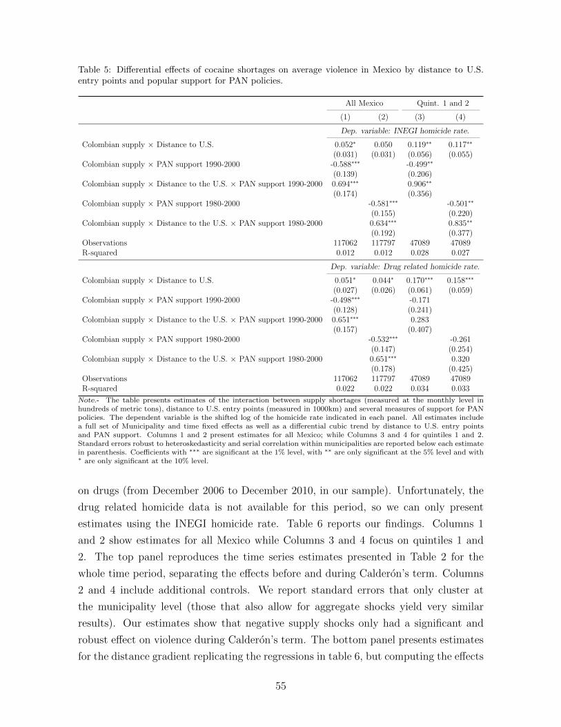
Table 5: Differential effects of cocaine shortages on average violence in Mexico by distance to U.S.entry points and popular support for PAN policies.
All Mexico Quint. 1 and 2
(1) (2) (3) (4)
Dep. variable: INEGI homicide rate.
Colombian supply × Distance to U.S. 0.052∗ 0.050 0.119∗∗ 0.117∗∗
(0.031) (0.031) (0.056) (0.055)Colombian supply × PAN support 1990-2000 -0.588∗∗∗ -0.499∗∗
(0.139) (0.206)Colombian supply × Distance to the U.S. × PAN support 1990-2000 0.694∗∗∗ 0.906∗∗
(0.174) (0.356)Colombian supply × PAN support 1980-2000 -0.581∗∗∗ -0.501∗∗
(0.155) (0.220)Colombian supply × Distance to the U.S. × PAN support 1980-2000 0.634∗∗∗ 0.835∗∗
(0.192) (0.377)Observations 117062 117797 47089 47089R-squared 0.012 0.012 0.028 0.027
Dep. variable: Drug related homicide rate.
Colombian supply × Distance to U.S. 0.051∗ 0.044∗ 0.170∗∗∗ 0.158∗∗∗
(0.027) (0.026) (0.061) (0.059)Colombian supply × PAN support 1990-2000 -0.498∗∗∗ -0.171
(0.128) (0.241)Colombian supply × Distance to the U.S. × PAN support 1990-2000 0.651∗∗∗ 0.283
(0.157) (0.407)Colombian supply × PAN support 1980-2000 -0.532∗∗∗ -0.261
(0.147) (0.254)Colombian supply × Distance to the U.S. × PAN support 1980-2000 0.651∗∗∗ 0.320
(0.178) (0.425)Observations 117062 117797 47089 47089R-squared 0.022 0.022 0.034 0.033
Note.- The table presents estimates of the interaction between supply shortages (measured at the monthly level inhundreds of metric tons), distance to U.S. entry points (measured in 1000km) and several measures of support for PANpolicies. The dependent variable is the shifted log of the homicide rate indicated in each panel. All estimates includea full set of Municipality and time fixed effects as well as a differential cubic trend by distance to U.S. entry pointsand PAN support. Columns 1 and 2 present estimates for all Mexico; while Columns 3 and 4 for quintiles 1 and 2.Standard errors robust to heteroskedasticity and serial correlation within municipalities are reported below each estimatein parenthesis. Coefficients with ∗∗∗ are significant at the 1% level, with ∗∗ are only significant at the 5% level and with∗ are only significant at the 10% level.
on drugs (from December 2006 to December 2010, in our sample). Unfortunately, the
drug related homicide data is not available for this period, so we can only present
estimates using the INEGI homicide rate. Table 6 reports our findings. Columns 1
and 2 show estimates for all Mexico while Columns 3 and 4 focus on quintiles 1 and
2. The top panel reproduces the time series estimates presented in Table 2 for the
whole time period, separating the effects before and during Calderon’s term. Columns
2 and 4 include additional controls. We report standard errors that only cluster at
the municipality level (those that also allow for aggregate shocks yield very similar
results). Our estimates show that negative supply shocks only had a significant and
robust effect on violence during Calderon’s term. The bottom panel presents estimates
for the distance gradient replicating the regressions in table 6, but computing the effects
55
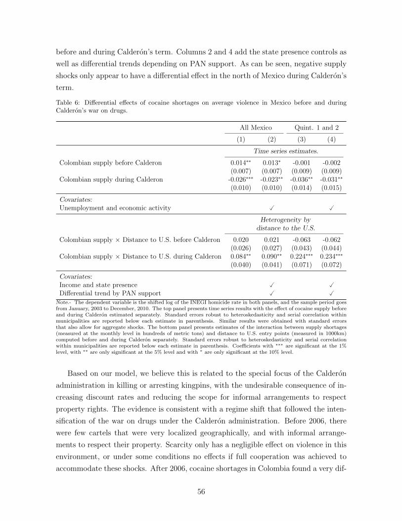
before and during Calderon’s term. Columns 2 and 4 add the state presence controls as
well as differential trends depending on PAN support. As can be seen, negative supply
shocks only appear to have a differential effect in the north of Mexico during Calderon’s
term.
Table 6: Differential effects of cocaine shortages on average violence in Mexico before and duringCalderon’s war on drugs.
All Mexico Quint. 1 and 2
(1) (2) (3) (4)
Time series estimates.
Colombian supply before Calderon 0.014∗∗ 0.013∗ -0.001 -0.002(0.007) (0.007) (0.009) (0.009)
Colombian supply during Calderon -0.026∗∗∗ -0.023∗∗ -0.036∗∗ -0.031∗∗
(0.010) (0.010) (0.014) (0.015)
Covariates:Unemployment and economic activity � �
Heterogeneity bydistance to the U.S.
Colombian supply × Distance to U.S. before Calderon 0.020 0.021 -0.063 -0.062(0.026) (0.027) (0.043) (0.044)
Colombian supply × Distance to U.S. during Calderon 0.084∗∗ 0.090∗∗ 0.224∗∗∗ 0.234∗∗∗
(0.040) (0.041) (0.071) (0.072)
Covariates:Income and state presence � �Differential trend by PAN support � �
Note.- The dependent variable is the shifted log of the INEGI homicide rate in both panels, and the sample period goesfrom January, 2003 to December, 2010. The top panel presents time series results with the effect of cocaine supply beforeand during Calderon estimated separately. Standard errors robust to heteroskedasticity and serial correlation withinmunicipalities are reported below each estimate in parenthesis. Similar results were obtained with standard errorsthat also allow for aggregate shocks. The bottom panel presents estimates of the interaction between supply shortages(measured at the monthly level in hundreds of metric tons) and distance to U.S. entry points (measured in 1000km)computed before and during Calderon separately. Standard errors robust to heteroskedasticity and serial correlationwithin municipalities are reported below each estimate in parenthesis. Coefficients with ∗∗∗ are significant at the 1%level, with ∗∗ are only significant at the 5% level and with ∗ are only significant at the 10% level.
Based on our model, we believe this is related to the special focus of the Calderon
administration in killing or arresting kingpins, with the undesirable consequence of in-
creasing discount rates and reducing the scope for informal arrangements to respect
property rights. The evidence is consistent with a regime shift that followed the inten-
sification of the war on drugs under the Calderon administration. Before 2006, there
were few cartels that were very localized geographically, and with informal arrange-
ments to respect their property. Scarcity only has a negligible effect on violence in this
environment, or under some conditions no effects if full cooperation was achieved to
accommodate these shocks. After 2006, cocaine shortages in Colombia found a very dif-
56
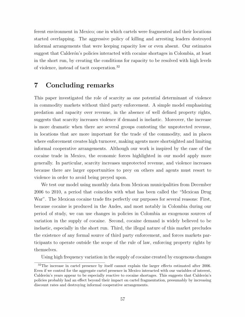
ferent environment in Mexico; one in which cartels were fragmented and their locations
started overlapping. The aggressive policy of killing and arresting leaders destroyed
informal arrangements that were keeping rapacity low or even absent. Our estimates
suggest that Calderon’s policies interacted with cocaine shortages in Colombia, at least
in the short run, by creating the conditions for rapacity to be resolved with high levels
of violence, instead of tacit cooperation.32
7 Concluding remarks
This paper investigated the role of scarcity as one potential determinant of violence
in commodity markets without third party enforcement. A simple model emphasizing
predation and rapacity over revenue, in the absence of well defined property rights,
suggests that scarcity increases violence if demand is inelastic. Moreover, the increase
is more dramatic when there are several groups contesting the unprotected revenue,
in locations that are more important for the trade of the commodity, and in places
where enforcement creates high turnover, making agents more shortsighted and limiting
informal cooperative arrangements. Although our work is inspired by the case of the
cocaine trade in Mexico, the economic forces highlighted in our model apply more
generally. In particular, scarcity increases unprotected revenue, and violence increases
because there are larger opportunities to prey on others and agents must resort to
violence in order to avoid being preyed upon.
We test our model using monthly data from Mexican municipalities from December
2006 to 2010, a period that coincides with what has been called the “Mexican Drug
War”. The Mexican cocaine trade fits perfectly our purposes for several reasons: First,
because cocaine is produced in the Andes, and most notably in Colombia during our
period of study, we can use changes in policies in Colombia as exogenous sources of
variation in the supply of cocaine. Second, cocaine demand is widely believed to be
inelastic, especially in the short run. Third, the illegal nature of this market precludes
the existence of any formal source of third party enforcement, and forces markets par-
ticipants to operate outside the scope of the rule of law, enforcing property rights by
themselves.
Using high frequency variation in the supply of cocaine created by exogenous changes
32The increase in cartel presence by itself cannot explain the larger effects estimated after 2006.Even if we control for the aggregate cartel presence in Mexico interacted with our variables of interest,Calderon’s years appear to be especially reactive to cocaine shortages. This suggests that Calderon’spolicies probably had an effect beyond their impact on cartel fragmentation, presumably by increasingdiscount rates and destroying informal cooperative arrangements.
57
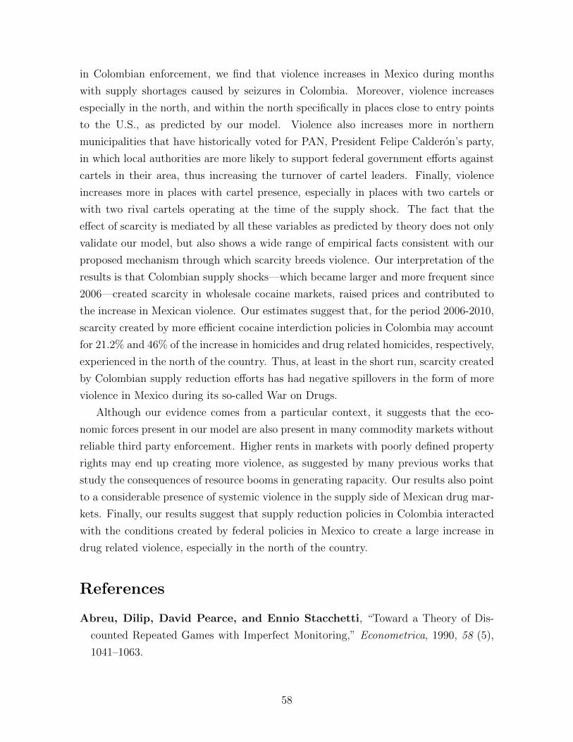
in Colombian enforcement, we find that violence increases in Mexico during months
with supply shortages caused by seizures in Colombia. Moreover, violence increases
especially in the north, and within the north specifically in places close to entry points
to the U.S., as predicted by our model. Violence also increases more in northern
municipalities that have historically voted for PAN, President Felipe Calderon’s party,
in which local authorities are more likely to support federal government efforts against
cartels in their area, thus increasing the turnover of cartel leaders. Finally, violence
increases more in places with cartel presence, especially in places with two cartels or
with two rival cartels operating at the time of the supply shock. The fact that the
effect of scarcity is mediated by all these variables as predicted by theory does not only
validate our model, but also shows a wide range of empirical facts consistent with our
proposed mechanism through which scarcity breeds violence. Our interpretation of the
results is that Colombian supply shocks—which became larger and more frequent since
2006—created scarcity in wholesale cocaine markets, raised prices and contributed to
the increase in Mexican violence. Our estimates suggest that, for the period 2006-2010,
scarcity created by more efficient cocaine interdiction policies in Colombia may account
for 21.2% and 46% of the increase in homicides and drug related homicides, respectively,
experienced in the north of the country. Thus, at least in the short run, scarcity created
by Colombian supply reduction efforts has had negative spillovers in the form of more
violence in Mexico during its so-called War on Drugs.
Although our evidence comes from a particular context, it suggests that the eco-
nomic forces present in our model are also present in many commodity markets without
reliable third party enforcement. Higher rents in markets with poorly defined property
rights may end up creating more violence, as suggested by many previous works that
study the consequences of resource booms in generating rapacity. Our results also point
to a considerable presence of systemic violence in the supply side of Mexican drug mar-
kets. Finally, our results suggest that supply reduction policies in Colombia interacted
with the conditions created by federal policies in Mexico to create a large increase in
drug related violence, especially in the north of the country.
References
Abreu, Dilip, David Pearce, and Ennio Stacchetti, “Toward a Theory of Dis-
counted Repeated Games with Imperfect Monitoring,” Econometrica, 1990, 58 (5),
1041–1063.
58
Acemoglu, Daron, James A. Robinson, and Rafael J. Santos, “The Monopoly of
Violence: Evidence from Colombia,” Journal of the European Economic Association,
2013, 11 (5-44).
Angrist, Joshua D. and Adriana D. Kugler, “Rural windfall or a new resourse
curse? Coca, income and civil conflict in Colombia,” The Review of Economics and
Statistics, May 2008, 90 (2), 191–215.
Arkes, Jeremy, Rosalie Liccardo Pacula, Susan M. Paddock, Jonathan P.
Caulkins, and Peter Reuter, “Why the DEA STRIDE Data are Still Useful for
Understanding Drug Markets,” NBER Working Paper No. 14224, 2008.
Bachman, Jerald G., Lloyd D. Johnston, and Patrick M. O’Malley, “Explain-
ing the Recent Decline in Cocaine Use among Young Adults: Further Evidence That
Perceived Risks and Disapproval Lead to Reduced Drug Use,” Journal of Health and
Social Behavior, 1990, 31, 173–184.
Becker, Gary S., “Crime and Punishment: An Economic Approach,” Journal of
Political Economy, 1968.
and Kevin M. Murphy, “A Theory of Rational Addiction,” Journal of Political
Economy, 1988, 96 (4), 675–700.
, , and Michael Grossman, “The Market for Illegal Goods: The Case of Drugs,”
Journal of Political Economy, 2006, 114 (1).
, Michael Grossman, and Kevin M. Murphy, “An Empirical Analysis of
Cigarette Addiction,” The American Economic Review, 1994, 84 (3), 397–418.
Bo, Ernesto Dal and Pedro Dal Bo, “Workers, warriors, and criminals: social
conflict in general equilibrium,” Journal of the European Economic Association, 2011,
9 (4), 646–677.
Bruckner, Markus and Antonio Ciccone, “International Commodity Prices,
Growth and the Outbreak of Civil War in Sub-Saharan Africa,” The Economic Jour-
nal, 2010, 120, 519–534.
Buonanno, Paolo, Ruben Durante, Giovanni Prarolo, and Paolo Vanin, “Poor
Institutions, Rich Mines: Resource Curse and the Origins of the Sicilian Mafia,”
Document de treball de l’IEB 2012-29, 2012.
Calderon, Gabriela, Alberto Diaz-Ceyros, and Beatriz Magaloni, “The Tem-
poral and Spatial Dynamics of Violence in Mexico,” MIMEO, Stanford University,
2012.
Cameron, Colin, Jonah B. Gelbach, and Douglas L. Miller, “Robust Inference
With Multiway Clustering,” Journal of Business and Economic Statistics, 2011, 29
(2).
59
Castillo, Juan Camilo, “Should drug policy be aimed at cartel leaders? Breaking
down a peaceful equilibrium,” Documento CEDE 2013-41, 2013.
Caulkins, Jonathan, “Estimating the Elasticities and Cross Elasticities of Demand
for Cocaine and Heroin,” Carnegie Mellon University working paper, 1995.
Chimeli, Ariaster B. and Rodrigo R. Soares, “The Use of Violence in Illegal
Markets: Evidence from Mahogany Trade in the Brazilian Amazon,” MIMEO, Uni-
versidade Catolica de Rio, 2010.
Collier, Paul and Anke Hoeffler, “Greed and Grievance in Civil War,” Oxford
Economic Papers, 2004, 56 (4), 563–595.
Coscia, Michele and Viridiana Rıos, “Knowing Where and How Criminal Orga-
nizations Operate Using Web Content,” in “CIKM ’12” Maui, HI, USA October
29-November 2 2012.
Couttenier, Mathieu, Pauline Grosjean, and Marc Sangnier, “The Wild West is
Wild: The Homicide Resource Course,” UNSW Australia Shool of Business working
paper, 2013.
Crawford, Neta C., “Civilian Death and Injury in Afghanistan, 2001-2011,” http://
costsofwar.org/sites/default/files/CrawfordAfghanistanCasualties.pdf
2011.
de la Sierra, Raul Sanchez, “On the Origin of States: Stationary Bandits and
Taxation in Eastern Congo,” University of Columbia working paper, 2014.
Dell, Melissa, “Trafficking Networks and the Mexican Drug War,” Job Market Paper,
November 2012.
DiNardo, John, “Law enforcement, the price of cocaine and cocaine use,” Mathemat-
ical and Computer Modeling, 1993, 17 (2), 53–64.
Dube, Arindrajit, Oeindrila Dube, and Omar Garcia Ponce, “Cross-border
Spillover: US Gun Laws and Violence in Mexico,” APSA 2012 Annual Meeting Paper,
2012.
Dube, Oeindrila and Juan Vargas, “Commodity Price Shocks and Civil Conflict:
Evidence from Colombia,” The Review of Economic Studies, 2013, 80 (41384-1421).
Elias, Norbert, The Civilising Process: State Formation and Civilisation, Wiley-
Blackwell, 2000.
Fearon, James D., “Primary Commodities Exports and Civil War,” Journal of Con-
flict Resolution, 2005, 49, 483–507.
and David D. Laitin, “Ethnicity, Insurgency, and Civil War,” American Political
Science Review., 2003, 97 (01).
Gambetta, Diego, The Sicilian Mafia: The Business of Private Protection, Harvard
60
University Press, 1996.
Garcıa-Jimeno, Camilo, “The Political Economy of Moral Conflict: An Empirical
Study of Learning and Law Enforcement under Prohibition,” University of Pennsyl-
vania working paper, 2012.
Goldstein, Paul J., “The Drugs/Violence Nexus: A Tripartite Conceptual Frame-
work,” Journal of Drug Issues, 1985, 39, 143–174.
Gonzalbo, Fernando Escalante, “Crimen organizado: La dimension imaginaria,”
Nexos, 2012.
Grillo, Ioan, El Narco, Bloomsbury Press, 2011.
Grosjean, Pauline, “A History of Violence: The Culture of Honor as a Determinant
of Homicide in the U.S. South,” Journal of the European Economic Association, 2013.
Grossman, Herschel I., “A General Equilibrium Model of Insurrections,” The Amer-
ican Economic Review, 1991, 81 (4), 912–921.
, “Kleptocracy and Revolutions,” Oxford Economic Papers, 1999, 51, 267–283.
, “The Creation of Effective Property Rights,” American Economc Reveiew P&P,
2001.
Guerrero, Eduardo, “Como reducir la violencia en Mexico,” Nexos, 2010.
, “La raız de la violencia,” Nexos, 2011.
, “Security, drugs and violence in Mexico: A survey,” 7th North American Forum,
2011.
Hirshleifer, Jack, “Conflict and rent-seeking success functions: Ratio vs. difference
models of relative success,” Public Choice, 1989, 63, 101–112.
, “The techonology of conflict as an economic activity,” The American Economic
Review, 1991, 81 (2), 130–134.
, “The Dark Side of the Force: Western Economic Association International 1993
Presidential Addres,” Economic Inquiry, 1994, 32 (1).
, The Dark Side of the Force: Economic Foundations of Conflict Theory, Cambridge
University Press, 2001.
Hobbes, Thomas, Leviathan 1651.
Horowitz, Joel L., “Should the DEA’s STRIDE Data Be Used for Economic Analyses
of Markets for Illegal Drugs?,” Journal of the American Statistical Association, 2001,
96 (456), 1254–1262.
Kalyvas, Stathis, The Logic of Violence in Civil War, Cambridge University Press,
2006.
Kilmer, Beau, Jonathan P. Caulkins, Brittany M. Bond, and Peter H.
Reuter, “Reducing Drug Trafficking Revenues and Violence in Mexico: Would Le-
61
galizing Marijuana in California Help?,” Rand Occasional Paper 325, 2010.
Levitt, Steven D. and Sudhir Alladi Venkatesh, “An economic analysis of a
drug-selling gang’s finances,” The Quarterly Journal of Economics, 2000, 115 (3),
755–789.
Lizarraga, Daniel, “Oculta el gobierno cifra de muertos en la
guerra contra el narco,” http://www.animalpolitico.com/2012/01/
oculta-el-gobierno-cifra-de-muertos-en-la-guerra-contra-el-narco/
#axzz2YBhYvry0 2012.
Mejıa, Daniel and Pascual Restrepo, “The War on Illegal Drug Production and
Trafficking: An Economic Evaluation of Plan Colombia,” Documento CEDE 2008-19,
2008.
and , “Do Illegal Drug Markets Breed Violence? Evidence for Colombia,”
MIMEO, Universidad de los Andes, May 2013.
Merino, Jose, “Los operativos conjuntos y la tasa de homicidios: Una medicion,”
Nexos, June 2011.
Miguel, Edward, Shanker Satyanath, and Ernest Sergenti, “Economic Shocks
and Civil Conflict: An Instrumental Variables Approach,” Journal of Political Econ-
omy, 1994, 112 (4), 725–753.
Nisbet, Charles T. and Firouz Vakil, “Some Estimates of Price and Expenditure
Elasticities of Demand for Marijuana Among U.C.L.A. Students,” The Review of
Economics and Statistics, 1972, 54 (4), 473–475.
Nisbett, Richard E. and Dov Cohen, Culture of Honor: The Psychology of Violence
in the South, Westview Press, 1996.
Owens, Emily G., “Are underground markets really more violent? Evidence from
early 20th century America,” American Law and Economics Review, 2011, 13 (1),
1–44.
, “The Birth of the Organized Crime? The American Temperance Movement and
Market-Based Violence,” Cornell working paper, 2011.
Pinker, Steven, The Better Angels of our Nature: Why Violence Has Declined, Viking
Adult, 2011.
Poire, Alejandro and Marıa Teresa Martınez, “La caıda de los capos no multiplica
la violencia: el caso de Nacho Coronel,” Nexos, 2011.
Proceso, “Pone gobierno ”bajo llave” cifras de ejecutados,” http://www.proceso.
com.mx/?p=293857 2012.
Ross, Michael L., “What Do We Know about Natural Resources and Civil War?,”
Journal of Peace Research, 2004, 41 (3), 337–356.
62
Rothemberg, Julio J. and Garth Saloner, “A supergame-theoretic model of price
wars during booms,” The American Economic Review, 1986, 76 (3), 390–407.
Roumasset, James and John Hadreas, “Addicts, Fences, and the Market for Stolen
Goods,” Public Finance Review, 1977, 5 (2), 247–272.
Saffer, Henry and Frank Chaloupka, “The Demand for Illicit Drugs,” Economic
Inquiry, 1999, 37 (3), 401–411.
Silverman, Lester P. and Nancy L. Spruill, “Urban crime and the price of heroin,”
Journal of Urban Economics, 1977, 4 (1), 80–103.
Skaperdas, Sergios, “Warlord Competition,” Journal of Peace Research, 2002, 39
(4), 435–446.
Skaperdas, Stergios, “Contest Success Functions,” Economic Theory, 1996, 7, 283–
290.
Thompson, Samuel B., “Simple formulas for standard errors that cluster by both
firm and time,” Journal of Financial Economics, 2011, 99, 1–10.
UNODC, World Drug Report, United Nations, 2013.
Valdes, Guillermo, Historia del Narcotrafico en Mexico, Aguilar, 2013.
Villalobos, Joaquın, “Nuevos mitos de la guerra contra el narco,” Nexos, 2012.
Wasserman, J., Willard G. Manning, J.P. Newhouse, and J.D. Winkler,
“The effects of excise taxes and regulations on cigarette smoking,” Journal of Health
Economics, 1991, 10 (1), 43–64.
Appendix A Robustness and other results
We now present some robustness checks and falsifications of our findings. These results
are not directly linked to the predictions of our theoretical model. Their purpose is
instead to support the validity of our empirical strategy.
A.1 Different transformations of the homicide rate
In order to deal with the logarithm of homicide rates that are equal to one, we shifted the
value of our dependent variable by the 90th percentile of the values in the database. The
reason why we chose this percentile is that, among other choices of percentiles, it results
in errors that are closest to normal. We would now like to show that our results do not
depend on this precise choice of percentile, or in the form of our transformation. In order
to do so, we first run our preferred regression (column 2 in table 3) by shifting homicide
rates by other percentiles. The first three columns in table 7 show our coefficient of
63
interest when shifting the homicide rate by the 90th, 50th and 10th percentile. In
column 4 we use another method to deal with municipalities with zero homicides:
we find homicide rates using the number of homicides plus one, and then find its
logarithm. This removes the arbitrariness of the percentile level used, but it has the
problem that one additional homicide is a large increase for municipalities with few
inhabitants. Column 5 uses the number of homicides without any transformation as
dependent variable. Columns 6 and 7 use Poisson and negative binomial models, which
are commonly used with count data. Finally, column 8 uses a binomial dependent
variable, which is when there are homicides in a given municipality, and zero otherwise.
Panel A shows that for all models the coefficient of interest is positive, and it is
significant at a high level, except for the regressions with the number of homicides and
the dummy as dependent variables, which anyway result in a coefficient that is signif-
icant at the 10% level. This is not surprising, since we believe that these models have
serious flaws: the regression with the number of homicides has errors with large tails
on the right, which leads to a high variance in the estimators, and the regression with
the homicides dummy does not capture increases in violence in the intensive margin.
For instance, municipalities with a large population, such as metropolitan zones, will
almost certainly have homicides during any given month, so this regression does not
capture changes in violence levels in these municipalities.
The different nature of each of the models mean that the coefficients of each of
the models are not comparable to each other. We therefore show the standardized
coefficients in panel B. All of them lie in the range between 0.0155 and 0.0232, except
for a clear outlier, the model with the homicides dummy as a dependent variable, which,
as explained above, has important flaws.
64
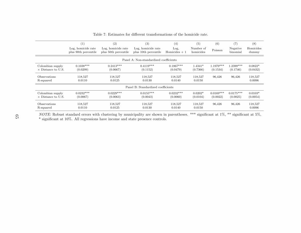
Table 7: Estimates for different transformations of the homicide rate.
(1) (2) (3) (4) (5) (6) (7) (8)
Log, homicide rate Log, homicide rate Log, homicide rate Log, Number ofPoisson
Negative Homicidesplus 90th percentile plus 50th percentile plus 10th percentile Homicides + 1 homicides binomial dummy
Panel A: Non-standardized coefficients
Colombian supply 0.1038*** 0.2413*** 0.4119*** 0.1867*** 1.4341* 1.1979*** 1.2399*** 0.0822*× Distance to U.S. (0.0299) (0.0667) (0.1152) (0.0479) (0.7366) (0.1534) (0.1746) (0.0432)
Observations 118,527 118,527 118,527 118,527 118,527 96,426 96,426 118,527R-squared 0.0110 0.0125 0.0130 0.0140 0.0150 0.0096
Panel B: Standardized coefficients
Colombian supply 0.0232*** 0.0229*** 0.0155*** 0.0232*** 0.0202* 0.0169*** 0.0175*** 0.0103*× Distance to U.S. (0.0067) (0.0063) (0.0043) (0.0060) (0.0104) (0.0022) (0.0025) (0.0054)
Observations 118,527 118,527 118,527 118,527 118,527 96,426 96,426 118,527R-squared 0.0110 0.0125 0.0130 0.0140 0.0150 0.0096
NOTE: Robust standard errors with clustering by municipality are shown in parentheses. *** significant at 1%, ** significant at 5%,* significant at 10%. All regressions have income and state presence controls.
65
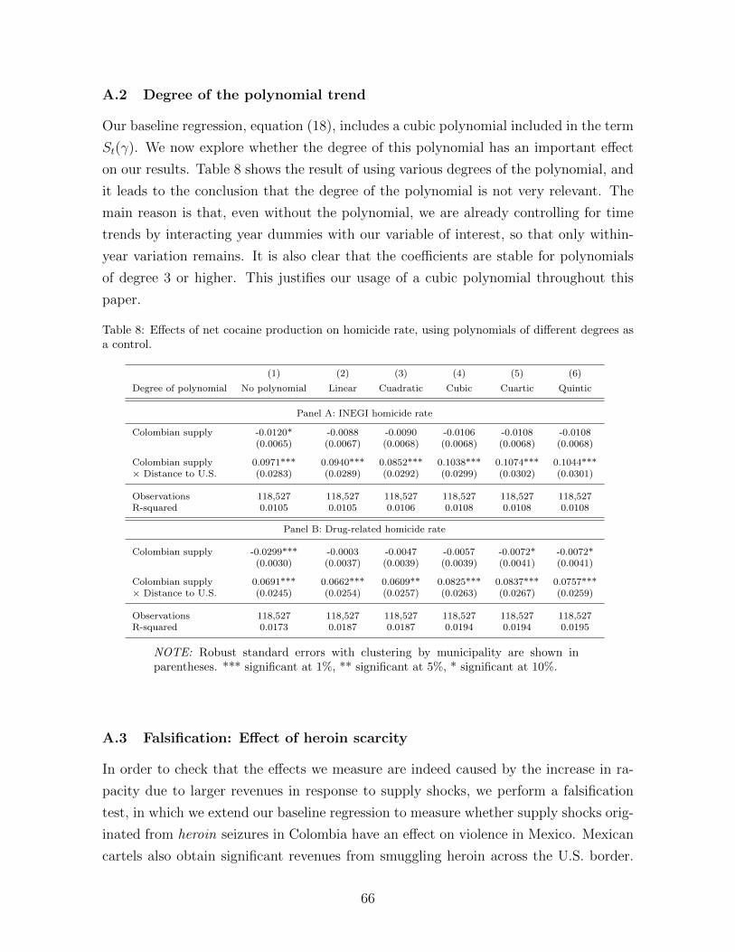
A.2 Degree of the polynomial trend
Our baseline regression, equation (18), includes a cubic polynomial included in the term
St(γ). We now explore whether the degree of this polynomial has an important effect
on our results. Table 8 shows the result of using various degrees of the polynomial, and
it leads to the conclusion that the degree of the polynomial is not very relevant. The
main reason is that, even without the polynomial, we are already controlling for time
trends by interacting year dummies with our variable of interest, so that only within-
year variation remains. It is also clear that the coefficients are stable for polynomials
of degree 3 or higher. This justifies our usage of a cubic polynomial throughout this
paper.
Table 8: Effects of net cocaine production on homicide rate, using polynomials of different degrees asa control.
(1) (2) (3) (4) (5) (6)
Degree of polynomial No polynomial Linear Cuadratic Cubic Cuartic Quintic
Panel A: INEGI homicide rate
Colombian supply -0.0120* -0.0088 -0.0090 -0.0106 -0.0108 -0.0108(0.0065) (0.0067) (0.0068) (0.0068) (0.0068) (0.0068)
Colombian supply 0.0971*** 0.0940*** 0.0852*** 0.1038*** 0.1074*** 0.1044***× Distance to U.S. (0.0283) (0.0289) (0.0292) (0.0299) (0.0302) (0.0301)
Observations 118,527 118,527 118,527 118,527 118,527 118,527R-squared 0.0105 0.0105 0.0106 0.0108 0.0108 0.0108
Panel B: Drug-related homicide rate
Colombian supply -0.0299*** -0.0003 -0.0047 -0.0057 -0.0072* -0.0072*(0.0030) (0.0037) (0.0039) (0.0039) (0.0041) (0.0041)
Colombian supply 0.0691*** 0.0662*** 0.0609** 0.0825*** 0.0837*** 0.0757***× Distance to U.S. (0.0245) (0.0254) (0.0257) (0.0263) (0.0267) (0.0259)
Observations 118,527 118,527 118,527 118,527 118,527 118,527R-squared 0.0173 0.0187 0.0187 0.0194 0.0194 0.0195
NOTE: Robust standard errors with clustering by municipality are shown inparentheses. *** significant at 1%, ** significant at 5%, * significant at 10%.
A.3 Falsification: Effect of heroin scarcity
In order to check that the effects we measure are indeed caused by the increase in ra-
pacity due to larger revenues in response to supply shocks, we perform a falsification
test, in which we extend our baseline regression to measure whether supply shocks orig-
inated from heroin seizures in Colombia have an effect on violence in Mexico. Mexican
cartels also obtain significant revenues from smuggling heroin across the U.S. border.
66
However, the large majority of the heroin they traffic is produced in Mexico (from
poppy cultivated in Mexico), especially in the states of Sinaloa, Michoacan, and Guer-
rero. According to the UNODC (2013), the potential heroin production in Mexico is
30 times higher than in Colombia. Therefore, heroin seizures in Colombia should have
no noticeable effects on the Mexican market, and thus should not increase rapacity
between Mexican cartels.
Our results are shown in table 9. In this exercise we use drug seizures in Colombia
instead of the net supply (as in all previous results) because there is no reliable estimate
of heroin production in Colombia that we can use to construct the net supply of heroin.
The coefficients should therefore have the opposite sign from the one shown in our main
results if the rapacity channel is present. Panels A and B show time series effects similar
to those shown in table 2 (so the coefficients should be positive), while panels B and
C show the differential effect of drug shortages with distance, similar to the results in
table 3 (so the coefficients should be negative). In the regressions of columns 2 and 4 we
include both cocaine and heroin seizures interacted with distance to the nearest border
crossing to the U.S. In all cases, coefficients for cocaine seizures remain almost the same
as without heroin seizures (columns 1 and 3). Furthermore, none of the coefficients for
heroin is significant, and the signs vary depending on the different regressions. We
interpret this as evidence in favor of our model, since heroin seizures in Colombia
cause no scarcity in Mexican drug markets that may increase violence through the
rapacity channel. This helps us conclude that there is no spurious correlation between
the high frequency behavior of drug seizures in Colombia and violence in Mexico—our
key identifying assumption—because there is only a measurable relationship between
violence and the type of drugs that would cause effects through the rapacity channel.
Appendix B Proof of proposition 2
Let gC(ai, Qs) be the maximum level of cooperation that can be sustained with a threat
of reversion to static Nash. Here, we focus only on symmetric equilibria. Let A(Qs) =(1 − η)siR(Qs) be a random variable describing vulnerable revenue in municipality i.The incentive compatibility constraint on this level is given by
1
NiA(Qs)−gC(ai, Q
s)+E
[ ∞∑t=1
βt(1− ai)t(gN (Qs)− gC(ai, Qs))
]≥ max
x
x
x+ (Ni − 1)gC(ai, Qs)A(Qs)−x.
(21)
Let Θ(ai) = E[∑∞
t=1 βt(1− ai)t(gN(Qs)− gC(ai, Q
s))]≥ 0. At this point, it is not
clear that this amount is uniquely determined for each value of Qs, but we will demon-
strate it below. The incentive compatibility constraint simply states that the gains from
67
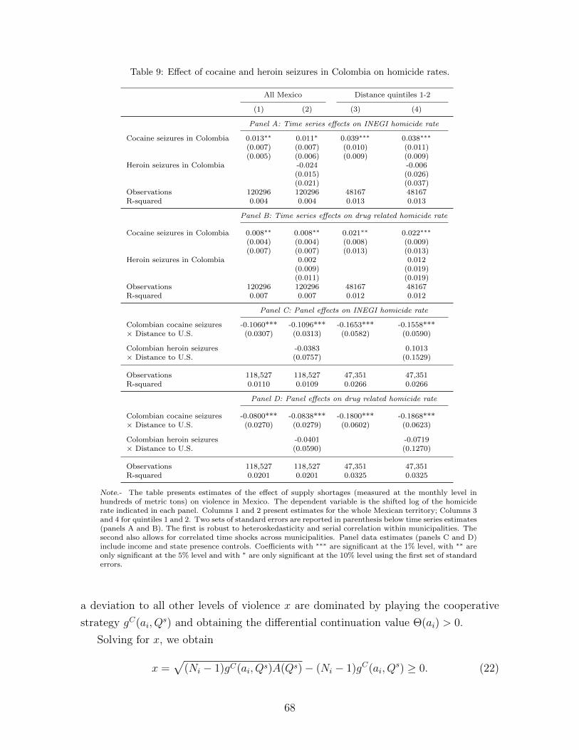
Table 9: Effect of cocaine and heroin seizures in Colombia on homicide rates.
All Mexico Distance quintiles 1-2
(1) (2) (3) (4)
Panel A: Time series effects on INEGI homicide rate
Cocaine seizures in Colombia 0.013∗∗ 0.011∗ 0.039∗∗∗ 0.038∗∗∗
(0.007) (0.007) (0.010) (0.011)(0.005) (0.006) (0.009) (0.009)
Heroin seizures in Colombia -0.024 -0.006(0.015) (0.026)(0.021) (0.037)
Observations 120296 120296 48167 48167R-squared 0.004 0.004 0.013 0.013
Panel B: Time series effects on drug related homicide rate
Cocaine seizures in Colombia 0.008∗∗ 0.008∗∗ 0.021∗∗ 0.022∗∗∗
(0.004) (0.004) (0.008) (0.009)(0.007) (0.007) (0.013) (0.013)
Heroin seizures in Colombia 0.002 0.012(0.009) (0.019)(0.011) (0.019)
Observations 120296 120296 48167 48167R-squared 0.007 0.007 0.012 0.012
Panel C: Panel effects on INEGI homicide rate
Colombian cocaine seizures -0.1060*** -0.1096*** -0.1653*** -0.1558***× Distance to U.S. (0.0307) (0.0313) (0.0582) (0.0590)
Colombian heroin seizures -0.0383 0.1013× Distance to U.S. (0.0757) (0.1529)
Observations 118,527 118,527 47,351 47,351R-squared 0.0110 0.0109 0.0266 0.0266
Panel D: Panel effects on drug related homicide rate
Colombian cocaine seizures -0.0800*** -0.0838*** -0.1800*** -0.1868***× Distance to U.S. (0.0270) (0.0279) (0.0602) (0.0623)
Colombian heroin seizures -0.0401 -0.0719× Distance to U.S. (0.0590) (0.1270)
Observations 118,527 118,527 47,351 47,351R-squared 0.0201 0.0201 0.0325 0.0325
Note.- The table presents estimates of the effect of supply shortages (measured at the monthly level inhundreds of metric tons) on violence in Mexico. The dependent variable is the shifted log of the homiciderate indicated in each panel. Columns 1 and 2 present estimates for the whole Mexican territory; Columns 3and 4 for quintiles 1 and 2. Two sets of standard errors are reported in parenthesis below time series estimates(panels A and B). The first is robust to heteroskedasticity and serial correlation within municipalities. Thesecond also allows for correlated time shocks across municipalities. Panel data estimates (panels C and D)include income and state presence controls. Coefficients with ∗∗∗ are significant at the 1% level, with ∗∗ areonly significant at the 5% level and with ∗ are only significant at the 10% level using the first set of standarderrors.
a deviation to all other levels of violence x are dominated by playing the cooperative
strategy gC(ai, Qs) and obtaining the differential continuation value Θ(ai) > 0.
Solving for x, we obtain
x =√
(Ni − 1)gC(ai, Qs)A(Qs)− (Ni − 1)gC(ai, Qs) ≥ 0. (22)
68
Plugging this value yields the incentive compatibility condition[1
Ni
− 1
]A(Qs) + Θ(ai) ≥ Nig
C(ai, Qs)− 2
√(Ni − 1)gC(ai, Qs)A(Qs). (23)
The right-hand side is decreasing for gC(ai, Qs) ∈ [0, gN(Qs)], and has a minimum at
gN(Qs). This implies that the above condition implies a lower bound for gC(ai, Qs), or
the smallest possible level of conflict that can be sustained with a reversion to static
Nash upon deviation.
Thus, the most cooperative equilibrium is given by the unique solution, gC(ai, Qs) ≥
0, to the functional equation[1
Ni
− 1
]A(Qs) + Θ(ai) ≥ Nig
C(ai, Qs)− 2
√(Ni − 1)gC(ai, Qs)A(Qs), (24)
with equality if gC(ai, Qs) > 0. Let Q(ai) be such that
(Ni − 1)A(Q(ai)) = NiΘ(ai). (25)
For Qs ≥ Q(ai), we have that the above condition holds as an inequality so
gC(ai, Qs) = 0 for large values of the supply Qs as stated in the proposition. If A(Qs)
is bounded, the above condition also holds as an inequality with gC(ai, Qs) = 0 when
β(1−ai)→ 1. Thus, for sufficiently low discounting there is always an equilibrium that
exhibits no violence along the equilibrium path if revenue is bounded. If, on the other
hand, revenue is unbounded, there is a sufficiently low Qs such that the above condition
does not hold for gC(ai, Qs) = 0, and we must have that gC(ai, Q
s) > 0 for sufficiently
low values of Qs. These observations establish the first two parts of the proposition.
Before continuing, we claim that Θ(ai) is decreasing in ai. We have that
Θ(ai) =β(1− ai)
1− β(1− ai)
(Ni − 1
N2i
E[A(Qs)]− E[gC(ai, Qs)]
). (26)
We have that for Qs < Q(ai),
gC(ai, Qs) =
(√(Ni − 1)A(Qs)−
√NiΘ(ai)
Ni
)2
. (27)
Plugging this in the above expression yields(1− β(1− ai)β(1− ai)
N2i +Ni
)√Θ(ai) = 2
√(Ni − 1)NiE
[√A(Qs)
]. (28)
This expression implies that Θ(ai) is unique (and hence the uniqueness of the solution)
69
and also that it is decreasing in ai as wanted. The above claim together with equation
25 also implies that Q(ai) is increasing in ai as mentioned in the first item of the
proposition. Using the formula for gc(ai, Qs) derived above, this also implies that gc is
increasing in ai as mentioned in the proposition.
Now, we focus on the role of Qs. so
∂gC(ai, Qs)
∂Qs=
(√(Ni − 1)A(Qs)−
√NiΘ(ai)
Ni
)√Ni − 1
A(Qs)A′s) < 0. (29)
The inequality follows from observing that for Qs < Q(ai) we have√
(Ni − 1)A(Qs) >√NiΘ(ai). In the above derivation it is key to notice that Θ(ai) does not depend on the
current realization of Qs because of the independence assumption on the draws. This
shows that violence increases when supply is tighter in this equilibrium as well. Thus,
informal arrangements are not enough to eliminate the impact of supply shortages on
violence when there is sufficient discounting and supply is tight enough.
Moreover, we have that∂2gC(ai, Q
s)
∂Qs∂ai< 0, (30)
because Θ(ai) is decreasing in ai. This proves the item of the proposition regarding the
cross partial derivative.
70