Scanner Data and Price Indexes - National Bureau of ... PDF is a selection from a published volume from the National Bureau of Economic Research Volume Title: Scanner Data and Price

This PDF is a selection from a published volume from theNational Bureau of Economic Research

Volume Title: Scanner Data and Price Indexes

Volume Author/Editor: Robert C. Feenstra and MatthewD. Shapiro, editors

Volume Publisher: University of Chicago Press

Volume ISBN: 0-226-23965-9

Volume URL: http://www.nber.org/books/feen03-1

Conference Date: September 15-16, 2000

Publication Date: January 2003

Title: The Measurement of Quality-Adjusted Price Changes

Author: Mick Silver, Saeed Heravi

URL: http://www.nber.org/chapters/c9739

277

9.1 Introduction

A major source of bias in the measurement of inflation is held to be its in-ability to properly incorporate quality changes (Boskin 1996; Boskin et al.1998; Diewert 1996; Cunningham 1996; Hoffmann 1998; Abraham, Green-less, and Moulton 1998). This is not to say statistical offices are unaware ofthe problem. Price collectors attempt to match the prices of “like with like”to minimize such bias. However, comparable items are often unavailable,and methods of implicit and explicit quality adjustment are not always con-sidered satisfactory (Reinsdorf, Liegey, and Stewart 1995; Armknecht,Lane, and Stewart 1997; Moulton, LaFleur, and Moses 1998).

Alongside this is an extensive empirical literature concerned with themeasurement of quality-adjusted price indexes at the product level. The

9 The Measurement ofQuality-Adjusted Price Changes

Mick Silver and Saeed Heravi

Mick Silver is professor of business statistics at Cardiff Business School, Cardiff University.Saeed Heravi is senior lecturer in quantitative methods at Cardiff Business School, CardiffUniversity.

This study is part of a wider project funded by the U.K. Office for National Statistics (ONS).The authors are grateful to the ONS for permission to reproduce some of this work in the formof this paper. The views expressed in the paper are those of the authors and not the ONS. Anyerrors and omissions are also the responsibility of the authors. Helpful advice during the work-ing of this paper was received from David Fenwick (ONS), Adrian Ball (ONS), Dawn Camus(ONS), and Pat Barr (GfK Marketing), and valuable programming assistance was receivedfrom Bruce Webb (Cardiff University). The paper has also benefited from useful commentsfrom Ernst Berndt (Massachusetts Institute of Technology), Erwin Diewert (University ofBritish Columbia), Rob Feenstra (University of California, Davis), John Greenlees (Bureauof Labor Statistics), Christos Ioannidis (Brunel University), Matthew Shapiro (University ofMichigan), and Ralph Turvey (London School of Economics). In particular, the authors hadsight of a draft Organization for Economic Cooperation and Development manual by JackTriplett (Brookings Institution), and this proved most useful for section 9.5, in which a varietyof approaches are used. The usual disclaimers apply.

main approach is the use of hedonic regressions (but see Blow and Craw-ford 1999 for an exception) in which the price of a model, for example, of apersonal computer is regressed on its characteristics. The data sources areoften unbalanced, panel cross-sectional time series from catalogs or webpages. A hedonic regression is estimated that includes the characteristics ofthe variety and dummy variables on time, the coefficients on the time dum-mies being estimates of the changes in price having controlled for changesin characteristics. This is referred to as the time dummy variable hedonicmethod. The quality-adjusted price index is taken from the coefficients onthe time dummies in the hedonic regression. There is usually little by way ofdata on quantities, and thus weights, in these estimates. Yet estimates fromhedonic regressions have been used to benchmark the extent of bias due toquality changes in consumer price indexes (CPIs; Boskin 1996; Boskin et al.1998; Hoffmann 1998).

In this first part of the paper (sections 9.2 to 9.4) we argue against the useof this widely adopted time dummy variable approach. It is set against the-oretical developments in the measurement of exact hedonic indexes byFixler and Zieschang (1992), Feenstra (1995), and Diewert (chap. 10 in thisvolume) and superlative index number formulas by Diewert (1976, 1978).The exact hedonic approach also uses hedonic regressions, but it differsfrom the time dummy hedonic approach in two ways. First, the coefficientson the quality characteristics are not restricted to be the same over time, asis the case with the time dummy variable method. Use is made of repeatedcross-section regressions in each period, rather than a single panel-data re-gression with dummy variables. Second, a formal sales weighting system isused in the exact approach, as opposed to implicit, equally weighted obser-vations. The exact approach also provides estimates of, and bounds for,cost-of-living indexes (COLI) based on economic theory. Cost-of-living in-dexes measure the ratio of the minimum expenditure required to maintaina given level of utility. The dummy variable approach is shown to be a re-stricted version of the exact hedonic approach. Concordant with the de-velopment of the theory for the exact hedonic approach has been devel-opments in data availability. Use is made of scanner data fromelectronic-point-of-sale bar code readings, which provide a sufficiently richsource to implement the exact hedonic approach and compare it with re-sults from the dummy variable method.

There are of course other variants of the time dummy variable method. Asales-weighted least squares estimator could be used, or estimates could bemade on a chained basis with, for example, a comparison between Januaryand February being based on hedonic regressions for these months only,with a time dummy for February, and similarly for February and March,March and April, and so on. The estimates of price changes over these bi-nary comparisons would be linked by successive multiplication to form achained estimate over the whole period.

278 Mick Silver and Saeed Heravi

Against all of this Turvey (1999a,b) has proposed, on pragmatic grounds,a matched method akin to that adopted by statistical offices. The availabil-ity of scanner data with information on the relative expenditure of eachproduct variety allows the compilation of matched indexes using exact andsuperlative formulas. The matched approach identifies the price of particu-lar varieties and compares this with the prices of the same varieties in sub-sequent periods. It thus reduces the need to use regressions for the mea-surement of quality-adjusted price changes since “like” is being comparedwith “like.” It is shown here how the exact hedonic approach based on Feen-stra (1995) and the matched approach are related, having respective prosand cons for the measurement of quality-adjusted COLI. Also provided areestimates, using scanner data, of quality-adjusted price indexes for washingmachines using all three of these approaches.

It is worth noting that scanner data are now available in Europe andNorth America for a wide range of consumer durables and fast-movinggoods. The coverage of the data is often quite extensive, being supple-mented by store audits for independent stores without bar code readers (seeHawkes and Smith 1999). Market research agencies including ACNielsonand GfK Marketing Services collate and supply such data. Their use for val-idation and other purposes is now recommended for the compilation ofconsumer price indexes by Boskin (1996) and for direct use by Diewert(1993) and Silver (1995).

There have been a number of studies using matching on this rich datasource in which prices of items with a particular specification are comparedwith their counterparts over time. These include Silver (1995), Saglio(1995), and Lowe (1999) for television sets and Reinsdorf (1996), Bradley etal. (1998), Haan and Opperdoes (1998), Dalen (1998), and Hawkes andSmith (1999) for selected food products. The matching used is often at ahighly disaggregated level, matching individual item codes with their coun-terparts over time. There have been fewer studies that compare the resultsof alternative methodologies: these include Silver’s (1999) study on TVs,which uses the dummy variable and exact hedonic approaches, and Moul-ton, LaFleur, and Moses’ (1999) and Kokoski, Waehrer, and Rozaklis’s(1999) studies on TVs and audio products, which use the dummy variableand hedonic quality-adjusted matching approaches. Studies, especiallythose using the dummy variable approach, invariably focus on a singlemethodology with little interest in the relationship between methods. Anearly and notable exception comparing the results from hedonic regressionsand matching, although not based on scanner data, was Cole et al. (1986).In this study we show how all three approaches are related and contrast theresults for the case of washing machines.

In section 9.2 we outline the three methods of measuring quality-adjusted price indexes and show how they are related. Section 9.3 providesa description of the data, the application in this study being to monthly data

The Measurement of Quality-Adusted Price Changes 279

on washing machines in the United Kingdom in 1998. The implementationof the three methods and their results are also outlined in section 9.3. Con-clusions on the appropriate method to measure quality-adjusted pricechanges using scanner data are in section 9.4.

The first part of the paper is concerned with how best to measure qual-ity-adjusted price changes given scanner data. The second part is an initialattempt to replicate the practice of statistical offices with regard to qualityadjustment. The same scanner data are used matching prices between prod-uct varieties in a base month, January, with their counterparts in February,and similarly for January with March, January with April, and so on. Whena product variety is missing in the current month, different variants of im-plicit and (hedonic) explicit adjustments are undertaken, as would be usedby a statistical office, and the results from these methods are compared. Themethodology is explained and the results are presented and discussed in sec-tion 9.5.

9.2 Quality-Adjusted Price Indexes: Three Approaches Using Scanner Data

This section outlines three methods for measuring quality-adjusted pricechanges using scanner data: the time dummy variable hedonic method, anexact hedonic approach, and a matching technique, which can utilize exactand superlative formulas. It is reiterated that

• both the time dummy and exact hedonic methods use hedonic regres-sions, the former using a single panel-data regression, whereas the lat-ter uses repeated cross-sectional ones;

• the time dummy hedonic method implicitly weights each observationequally in the regression, whereas the exact indexes have weighted for-mulations;

• the need for hedonic regressions is reduced when matching is effective.

9.2.1 Time Dummy Variable Hedonic Method

The hedonic approach involves the estimation of the implicit, shadowprices of the quality characteristics of a product. Products are often sold bya number of manufacturers, who brand them by their “make.” Each makeof product is usually available in more than one model, each having differ-ent characteristics. A set of (zk � 1, . . . K ) characteristics of a product isidentified, and data over i � 1, . . . N product varieties (or models) over t �1, . . . , T periods are collected. A hedonic regression of the price of modeli in period t on its characteristics set ztki is given by

(1) pti � �0 � ∑T

t�2

�tDt � ∑K

k�1

�kztki � εti


where Dt is a dummy variable for the time periods, D2 being 1 in period t �2, zero otherwise; D3 being 1 in period t � 3, zero otherwise, and so on.

The coefficients �t are estimates of quality-adjusted price changes, that is,estimates of the change in the price between period 1 and period t, havingcontrolled for the effects of variation in quality (via ∑K

k�1�kztki ).The theoretical basis for the method has been derived in Rosen (1974), in

which a market in characteristic space is established (see also Triplett 1987;Arguea, Haseo, and Taylor 1994). There is a plethora of studies of the aboveform as considered by Griliches (1990), Triplett (1990), and Gordon (1990),but subsequently including Nelson, Tanguay, and Patterson (1994); Gandal(1994, 1995); Arguea, Haseo, and Taylor (1994); Lerner (1995); Berndt,Griliches, and Rappaport (1995); Moulton, LaFleur, and Moses (1999);Hoffmann (1998); and Murray and Sarantis (1999). An issue of specificconcern is the choice of functional form to be used. There has been supportfor, and success in, the use of the linear form, including Arguea, Haseo, andTaylor (1994); Feenstra (1995); Stewart and Jones (1998); and Hoffmann(1998). The semilog formulation has also been successfully used in studiesincluding Lerner (1995); Nelson, Tanguay, and Patterson (1994); and Moul-ton, LaFleur, and Moses (1999). Studies using, and testing for, more com-plex functional forms have been advocated by Diewert (chap. 10 in this vol-ume) and generally applied to housing (Rasmussen and Zuehlke 1990; Millsand Simenauer 1996) with some success, such studies for consumer durablegoods (using flexible functional forms and neural networks; Curry, Morgan,and Silver 2001) being more limited.

The data sources used may be scanner data but are often specialist mag-azines or mail-order catalogs. The approach as conventionally used is notwithout problems. First, it implicitly treats each model as being of equal im-portance, when some models will have quite substantial sales, whereas forothers sales will be minimal. If data are available on sales values, a weightedleast squares estimator may be employed (Ioannidis and Silver 1999). Sec-ond, the prices recorded are not the transaction price averaged over a rep-resentative sample of types of outlets, but often a single, unusual supplier.

A final problem arises with the manner in which the time dummy variablemethod takes account of changing marginal values (coefficients) over time.It is the usual practice that the coefficients are held constant and thus notallowed to reflect changes in the marginal worth of the characteristics.Dummy slope coefficients on each characteristic for each period would re-lax the constraint. Yet this would render the estimate of quality-adjustedprice changes, the coefficient on the dummy (time) intercept, dependent onthe values of the performance characteristics (Silver 1999; Kokoski,Waehrer, and Rozaklis 1999). We will see that the above problems are dealtwith in the exact hedonic formulation, the dummy variable hedonic methodbeing a restricted version of the exact hedonic approach.


9.2.2 Exact (and Superlative) Hedonic Indexes

Konüs (1939) and Diewert (1976) define a theoretical COLI, Pc , as theratio of the minimum expenditure required to achieve a given level of util-ity, U, when the consumer faces period t prices compared with period t – 1price, pt , and pt–1 ; that is,

(2) Pc( pt, pt�1, U ) � �E

E

(

(

p

p

t�

t ,

1,

U

U

)

)�

The above does not recognize that changes may occur in the quality mix ofthe items compared. Fixler and Zieschang (1992) and Feenstra (1995) de-fine an analogous hedonic COLI:

(3) Pc( pt , pt�1, zt, zt�1, U ) ��E(

E

p

(

t�

p

1

t

,

,

z

z

t

t

�

,

1

U

, U

)

)�

that is, the ratio of the minimum expenditure required to maintain a givenlevel of utility when the consumer faces pt and pt–1 prices and quality char-acteristics zt and zt–1.

The construction of such indexes requires the existence of a representa-tive consumer whose expenditure functions are defined over the space of“characteristics,” prices, and utility. When goods differ in their characteris-tics and consumers are heterogeneous in their preferences, only a specificclass of functions describing the behavior of agents can be aggregated tosome “representative” agent.

Theoretical frameworks are given by Feenstra (1995) and Diewert (chap.10 in this volume). Feenstra uses aggregation results from McFadden(1983) to show that a representative agent formulation indeed arises from adiscrete choice model, in which the individual consumers are decidingwhich of a discrete number of alternative varieties to choose. Feenstra pro-poses a reasonably broad class of utility functions for the individual con-sumers, which has two components: a subutility function over characteris-tics zi � RK

� , which is the same across consumers; and an additive termobtained from each variety chosen, which differs across consumers. The lat-ter additive terms are modeled as random across consumers, with a general“extreme value” distribution. Any pattern of correlation in the utility ob-tained from different models is allowed for, so this framework is much moregeneral than the multinominal logit model, for example (in which the addi-tive errors obtained from each variety are independent).

In this context, there exists an expenditure function for the representativeconsumer, E( pt , zt, Ut ), where pt � (p1t , . . . pNt ) is the vector of prices for theN varieties, and zt � (z1t , . . . zNt ) is the NK-dimensional vector of charac-teristics over all the product varieties. Social welfare, Ut , is interpreted as thesum of utilities over the individual consumers (i.e., utilitarian social wel-fare), and E( pt , zt, Ut ), measures the minimum expenditure summed over all


consumers to obtain Ut . For each variety, we can also define the marginalvalue of characteristics to consumers, �i � RK

�, which is the same across con-sumers. As characteristics change over time, bounds for the exact index canbe constructed using these values. The current (Paasche) period and base(Laspeyres) weighted quality-adjusted bounds for a COLI, for an arith-metic aggregation using a linear hedonic equation, are given by Feenstra(1995) as

(4a) ��∑∑Ni�

Ni�

1x1x

it

i

ptp

ˆit�

it

1

��E(

E

p

(

t�

p

1

t

,

,

z

z

t

t

�

,

1

U

, U

)

)�� ∑∑N

i�

Ni�

1x1x

it�

it�

1p1p

it�

it

1

��where E(�) denotes the expenditure function, at periods t and t – 1, evalu-ated at a fixed level of utility, and the arguments in the index are given by

(4b) pit � pit � ∑�kt(zikt � zikt�1)

pit�1 � pit�1 � ∑�kt�1(zikt � zikt�1)

where Laspeyres and Paasche in equation (4a) are upper and lower boundson their “true”, economic theoretic COLIs: x is quantity sold, p is price, andz is a vector of characteristics with associated marginal values �kit derivedfrom a linear hedonic regressions over i � 1 . . . N product varieties (mod-els) for each period t. Changes in the quality of models are picked up viachanges in their characteristics (zkt – zkt–1), which are multiplied by estimatesof their associated marginal values �kt . With sales data available, the vectorz can be the sales-weighted average usage or mix of each characteristic ineach period. Note that pit corrects the observed prices pit for changes in thecharacteristics between the two periods, corresponding to the “explicitquality adjustment” described by Triplett (1990, 39).

Equation (4) has a simple intuition. In equation (4a) matched prices arebeing compared using current period quantities (weights) on the left-handside and base period quantities on the right-hand side of the equation.However, the matching may not be perfect in that for each i, the quality maychange over time. Consequently, predicted values are generated in equa-tions (4b) to correct for such changes. For the left-hand side they adjust thebase period prices for changes in the characteristics taking place between t–1 and t: maybe the goods are getting better over time. This change for eachi is �zik � (zikt – zikt–1), where zikt is the sales-weighted average of each k qual-ity characteristic: say, the average spin speed or load capacity of washingmachines has increased. However, some characteristics are more impor-tant, in a price-determining sense, than others, so each �z is weighted by anestimate of its marginal value from a hedonic regression. For the left-handside the hedonic regression is estimated using base period t – 1 data to cor-rect pt–1, and for the right-hand side current period t data are used to correctpt . It will be shown later how the i has to be defined in practice as productgroups in which the quality mix changes but the intuition remains.


Economic theory provides further help with the choice between indexnumber formulas. Cost-of-living index number formulas are defined in eco-nomic theory as exact for particular types of preferences if they equal theratio of expenditure required to maintain constant utility for consumerswith those types of preferences. Different index number formulas have beenshown to have an exact correspondence to the functional form of the con-sumer’s expenditure function. Laspeyres and Paasche price indexes (equa-tion [4a]) correspond to fixed coefficient Leontief forms and act as upperand lower bounds on a true COLI. Base and current period weighted geo-metric means indexes could also be calculated, these being exact for (corre-sponding to) utility-maximizing consumers with constant elasticity of sub-stitution (Feenstra 1995 and footnote 1). Diewert (1976, 1978) found thatsymmetric averages of these bounds provide index number formulas thatcorrespond to flexible functional forms for the expenditure function, whichare much less restrictive. He defined such index number formulas as beingsuperlative. Fisher’s index is the geometric mean of Laspeyres and Paascheand is superlative. The Törnqvist index1 uses a symmetric mean of theweights of the bounds in equation (4a) and is superlative and exact for (cor-responds to) a flexible translog utility function. Fisher’s and Törnqvist in-dexes are thus quite special in that they are superlative, although Diewert(1995, 1997) has also shown the two formulas to be superior to many oth-ers from an axiomatic approach, with Fisher’s in particular satisfying more“reasonable” tests than its competitors. The exposition here has been forarithmetic aggregation as opposed to a geometric one, although the resultsfor geometric bounds and a Törnqvist index are noted in section 9.4 and areavailable from the authors.

The advantages of the exact hedonic approach are threefold. First, it uti-lizes the coefficients on the characteristics in an unconstrained manner toadjust observed prices for quality changes. Second, it incorporates aweighting system using data on the sales of each model and their charac-teristics, rather than treating each model as equally important. Finally, ithas a direct correspondence to a constant utility index number formulationdefined from theory.

9.2.3 Matching

We finally consider the process of matching. It compares the prices ofmatched identical varieties over time, so that the pure price changes are nottainted by quality changes. The aim is to compare only like with like. Thisis akin to the process used by price collectors for statistical offices in the


1. The geometric current and base-period bounds are given by ΠNi�1(pit /pit–1)

sit � [E(pt , zt, U )]/[E(pt–1, zt–1, U )] � ΠN

i�1( pit /pit–1 )sit–1, where pit–1 � pit–1 exp[∑�kt–1(zikt – zikt–1)] and pit � pit exp[–∑�kt(zikt – zikt–1)], and the Törnqvist index is given by Π(pt /pt–1)[(wt�wt–1)/2] � [Π( pt /pt–1)

wt Π( pt /pt–1)wt–1]1/2, where wt � ( ptxt /∑ptxt) and wt–1 � ( pt–1xt–1/∑pt–1xt–1).

compilation of CPIs, but the matching is electronic using scanner data.Scanner data have a code to describe each model of a good. The code canbe extended to include the type of outlet in which it is sold, in order that aparticular model of a good in a particular type of outlet is matched againstits counterpart in successive periods. Since individual retailers often haveunique codes for the same model, the matching is in practice closer than by“model and outlet type.” The problem with such matching is missing ob-servations. For scanner data they arise when there is no transaction in thatoutlet (type) in a period, possibly because the item is no longer being soldor is on display but has not been bought.2

Turvey (1999a) proposed the use of chained matched indexes wherebythe aggregate price change between, for example, January and February isspliced to that for February and March and so forth by successive multipli-cation. For example, the chained index between January and December,CIJ,D , is given by the product of the individual successive binary comparisons:

(5) CIJ,D � IJ,F IF,M IM,A . . . IN,D

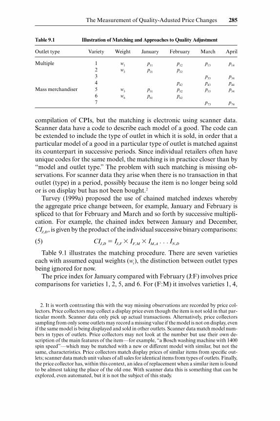
Table 9.1 illustrates the matching procedure. There are seven varietieseach with assumed equal weights (wi ), the distinction between outlet typesbeing ignored for now.

The price index for January compared with February (J:F) involves pricecomparisons for varieties 1, 2, 5, and 6. For (F:M) it involves varieties 1, 4,


Table 9.1 Illustration of Matching and Approaches to Quality Adjustment

Outlet type Variety Weight January February March April

Multiple 1 w1 p11 p12 p13 p14

2 w2 p21 p22

3 p33 p34

4 p42 p43 p44

Mass merchandiser 5 w5 p51 p52 p53 p54

6 w6 p61 p62

7 p73 p74

2. It is worth contrasting this with the way missing observations are recorded by price col-lectors. Price collectors may collect a display price even though the item is not sold in that par-ticular month. Scanner data only pick up actual transactions. Alternatively, price collectorssampling from only some outlets may record a missing value if the model is not on display, evenif the same model is being displayed and sold in other outlets. Scanner data match model num-bers in types of outlets. Price collectors may not look at the number but use their own de-scription of the main features of the item—for example, “a Bosch washing machine with 1400spin speed”—which may be matched with a new or different model with similar, but not thesame, characteristics. Price collectors match display prices of similar items from specific out-lets; scanner data match unit values of all sales for identical items from types of outlets. Finally,the price collector has, within this context, an idea of replacement when a similar item is foundto be almost taking the place of the old one. With scanner data this is something that can beexplored, even automated, but it is not the subject of this study.

and 5, for (M:A) the same three varieties and, in addition, varieties 3 and 7.The sample composition changes for each comparison as varieties die andare born. The results for each comparison are chained to provide a single in-dex for the whole period. Turvey advocates a chained geometric mean ofmatched observations.

Where wholly new products reflecting rapid technical improvement areintroduced into a market, overlap price ratios between old and new prod-ucts usually change from month to month. Instead of proceeding asabove, arbitrarily selecting just one month’s overlap price ratio betweena replacement product and the replaced product, this procedure takesinto account the ratio during all overlap months so that the prices of boththe old and new products enter into the index computation. When newproducts arrive on the market their prices should be brought into the in-dex, the prices of old products only being removed from it when they dis-appear from the market. Thus a chained geometric index of matched ob-servations will be used with a sample size which varies through time.(Turvey 1999a, 13)

The method involves some loss of information. No use, for example, ismade of p42 for (J:F), and of p22, p33, p62, and p73 for the (F:M) price compar-isons, which is naturally to be regretted. This is to allow constant qualitycomparisons. However, it is on the birth and death of a product that pricechanges are unusual, and these are the very ones lost.3 Some care, however,is needed in such statements. Table 9.1 illustrates how the loss of a matchedobservation takes place. For variety 2 in table 9.1, p22 is used for the Januaryto February comparison, so it is not lost here. However, it is lost in thematching for the February to March comparison. It is tempting to arguethat this loss is unimportant. It relates to a meaningless comparison be-cause it does not exist in March and there is thus no basis for a price com-parison. However, economic theory would assert otherwise. The economicsof new goods is quite clear on the subject. If a new good is introduced, it isnot sufficient to simply wait for two successive price quotations and then in-corporate the good. This would ignore the welfare gain to consumers asthey substitute from old technology to new technology. Such welfare gainsare inseparably linked to the definition of a COLI defined as indexes, whichmeasure the expenditure, required to maintain a constant level of utility(welfare). There exists in economic theory and practice the tools for the es-timation of such effects (Hicks 1940; Diewert 1980, 498–503). This involvessetting a “virtual” price in the period before introduction. This price is theone at which demand is set to zero. The virtual price is compared with theactual price in the period of introduction, and this is used to estimate the


3. A parallel issue arises for indexes of industrial production, especially in less developedcountries, where new products are often new industries and ignoring their contribution to pro-duction when they are set up may seriously understate growth (Kmietowicz and Silver 1980).

welfare gain. Hausman (1997) provides some estimates for the introductionof a new brand of Apple-Cinnamon Cheerios. He concludes:

The correct economic approach to the evaluation of new goods has beenknown for over fifty years since Hicks’s pioneering contribution. How-ever, it has not been implemented by government statistical agencies, per-haps because of its complications and data requirements. Data are nowavailable. The impact of new goods on consumer welfare appears to besignificant according to the demand estimates of this paper; the CPI forcereal may be too high by about 25 percent because it does not accountfor new cereal brands. An estimate this large seems worth worrying about.

Notwithstanding this, a curious feature of scanner data is that a missingtransaction may arise simply because a model has not been purchased butis still on sale. A price collector would pick up the missing sales price notknowing it is above its reservation price, and there will thus be no need toestimate a virtual price.

9.2.4 Correspondence between the Methods

Matched versus Exact Hedonic Indexes

There is an interesting and useful correspondence here. Consider equa-tion (4b). The pt is the price (or unit value) of model i (in a given outlet) inperiod t, having been adjusted by changes in its quality characteristics be-tween period t – 1 and t, the change in each characteristic being weightedby its associated marginal value in period t. If we are matching, no suchadjustment is necessary. Matching does, however, have its failings in thatinformation is lost. The exact hedonic formulation, as undertaken here inpractice, aggregates not over each model, but over a subset of meaningfulcharacteristics. For washing machines, for example, we might use makesand outlet types. The Laspeyres formulation on the right-hand side of equa-tion (4) may be approximated by

(6a)

where we define a narrow set of Gj characteristics—say, dummy variablesfor makes and outlet types—that are present in most models of the productin each period, where j � 1 . . . J combinations of makes and outlet types.The p� and x in equation (6a) are now the average prices and total quantitiesfor each make in each outlet type, for example, for Zanussi washing ma-chines sold in multiples, within a make and outlet type j for each period t.The adjusted average price for models i in each j in period t is given by

(6b) p�jt = p�jt � �∑i�Gj

�1t�z�j1t � ∑i�Gj

�2t�z�j2t � . . . ∑i�Gj

�Kt�z�jKt�

∑Jj�1xjt�1 p�jt

��∑J

j�1xjt�1p�jt�1


where p�jt is the sales-weighted average price for each j make in a particularoutlet type, �z�jkt � (z�jkt – z�jkt–1), where z�jkt and z�jkt–1 are sales-weighted aver-ages (in each period) of the k characteristics other than makes and outlets(e.g., spin speed) and �k is their estimated marginal value. In equation (6a)for, say, group j � 1, Zanussi washing machines in multiples, the averageprice in period t, p�jt , is compared with that in period t – 1, p�jt–1. However, thequality of such machines may have changed over the period. This is ad-justed for in equation (6b). For each j, say, j � 1, the quality-adjusted aver-age price p�jt in period t is the (sales-weighted) mean price of varieties in thatgroup minus (adjusted for) the change in quality. For example, �z1t might bethe change in the (sales-weighted) average spin speed of washing machinesfor that make or outlet type, multiplied by an estimate in period t, of themarginal value of a unit of spin speed from an hedonic regression. The sum-mation is over the i varieties that are members of the j � 1 group. These ad-justments continue for other quality characteristics z2 . . . zk in equation(6b). The pp�jt are thus quality-adjusted within each of the groups being ag-gregated in equation (6a). The more quality characteristics we aggregateover in the body of equation (6a), the fewer characteristics are used in de-termining pp� in (6b). Equation (6a) should collapse down to the matchedmethod, when aggregating over all characteristics. So why restrict the ag-gregation in (6a) to only makes and outlet types? The answer is that in do-ing so we use all the data. On matching in table 9.1 we lost p33 for the Feb-ruary to March comparison but regained it for March to April.

Note that there is a minimal loss of information in the exact hedonic for-mulation given by equation (6) because each model has a make and outlettype. There is an efficiency gain to the estimate akin to that from stratifiedsampling in which we correct for quality changes by matching for pricechanges between strata and use estimates within strata. If we aggregatedover all characteristics in equation (6a), with no adjustments in (6b) wewould have a matching process with some models having no price datafor either period t or t – 1 in any two-way comparison. These would beexcluded. However, when we allow the aggregation over a limited numberof characteristics, which include models available in both periods, no in-formation is lost. The adjustment for the variables not included in thisweighted aggregation takes place in ppp�. There is a trade-off. The more qual-ity variables in the weighted aggregation, the more chance of losing infor-mation. We consider this in the empirical section.

Both the exact hedonic and matching approaches allow all forms ofweighting systems, including Laspeyres, Paasche, and the superlativeFisher, to be used to gain insights into such things as substitution effects.The exact hedonic formulation uses statistical estimates of product “worth”to partial out quality changes for the characteristics excluded in the aggre-gation in equation (6a), rather than the more computational, and accurate,matching. The differences between the methods depend on the reliability of


the p� adjustment process, in terms of both the extent of changes in charac-teristics (�z) and the values of �, and the relative loss of observations inbringing these characteristics into the aggregation process. Its extent is anempirical matter, and we will investigate this.

The equivalence of the two methods requires that the exact hedonic indextake a chained formulation, as is the case for the matched approach. Thechained approach has been justified as the natural discrete approximationto a theoretical Divisia index (Forsyth and Fowler 1981). Reinsdorf (1998)has formally determined the theoretical underpinnings of the index, con-cluding that in general chained indexes will be good approximations to thetheoretical ideal—although they are prone to bias when prices changes“swerve and loop,” as Szulc (1983) has demonstrated (see also Haan andOpperdoes 1998).

Direct versus Exact Hedonic

We include in the analysis results of the time dummy variable method,given its use in many studies and the taking of such estimates as indicatorsof potential errors due to lack of quality adjustment in CPIs (Boskin 1996;Hoffman 1998). However, as argued in Silver (1999), it is but a limited formof the exact hedonic approach, the limitations naturally arising from thelimited catalog data upon which the estimates are often based and the ab-sence of sales weights. Consider the time dummy variable method if we,first, used weighted average prices on the left-hand side of equation (1) anda sales-weighted least squares estimator and, second, introduced dummyslope variables for each characteristic against time to allow for changingmarginal values. The improved specification would require estimates of thechange in quality-adjusted price change to be conditioned on the change incharacteristics. If we take the value-weighted mean usage of each charac-teristic as the average usage upon which the change in quality-adjustedprices is conditioned, we have a framework akin to the exact hedonic one.Each of the modifications outlined above is just a relaxation of a restrictiveassumption of the time dummy variable approach. We nonetheless includein this study estimates from the time dummy variable approach in order toidentify the extent of errors arising from its conventional use.

9.3 Data and Implementation

9.3.1 Data

Scope and Coverage

The study is for monthly price indexes for washing machines in 1998 us-ing scanner data. Scanner data are compiled on a monthly basis from thescanner (bar code) readings of retailers. The electronic records of just aboutevery transaction include the transaction price, time of transaction, place of


sale, and a code for the item sold—for consumer durables we refer to this asthe model number. Manufacturers provide information on the quality char-acteristics, including year of launch, of each model that can then be linkedto the model number. Retailers are naturally interested in analyzing marketshare and pass on such data to market research agencies for analysis. By cu-mulating these records for all outlets (which are supplemented by visits toindependent outlets without scanners) the agencies can provide compre-hensive data on a monthly basis for each model for which there is a trans-action, on the following: price (unit value), volume of sales, quality charac-teristics, make, and outlet type. Agencies are reluctant to provide separatedata for a given model in a given outlet. This would not only allow com-petitors to identify how each outlet is pricing a particular model, and the re-sulting sales, but also allow manufacturers and governmental and otherbodies to check on anticompetitive pricing. Data are, however, identifiableby broad types of outlets, and model codes often apply to specific outlets,although they are not identifiable.

It should be noted that the data, unlike those collected by price collectors,possess the following characteristics:

• They cover all time periods during the month. • They capture the transaction price rather than the display price. • They are not concerned with a limited number of “representative”

items. • They are not from a sample of outlets. • They allow weighting systems to be used at an elementary level of ag-

gregation. • They include data on quality characteristics. • They come in a readily usable electronic form with very slight potential

for errors.

The data are not without problems, in that the treatment of multibuysand discounts varies between outlets and the coverage varies between prod-uct groups. For example, items such as cigarettes, which are sold in a vari-ety of small kiosks, are problematic. Nonetheless, they provide a recognizedalternative, first proposed by Diewert (1993) and used by Silver (1995) andSaglio (1995), but see also, for example, Lowe (1998) for Canada and Moul-ton, LaFleur, and Moses (1999) and Boskin (1996) for the United States. AsAstin and Sellwood (1998, 297–98) note in the context of Harmonised In-dices of Consumer Prices (HICP) for the European Union:

Eurostat attaches considerable importance to the possible use of scannerdata for improving the comparability and reliability of HICPs ([Euro-pean Union] Harmonised Indices of Consumer Prices), and will be en-couraging studies to this end. Such studies might consider the variousways in which scanner data might be used to investigate different issuesin the compilation of HICPs for example . . . provide independent esti-mates as a control or for detection of bias in HICP sub indices; . . .


analyse the impact of new items on the index; [and] carry out research onprocedures for quality control.

Our observations (observed values) are for a model of the product in agiven month in one of four different outlet types: multiples, mass merchan-disers, independents, and catalog. We stress that we differentiate models asbeing sold in different types of outlets. This is a very rich formulation sinceit allows us to estimate, for example, the marginal value of a characteristicin a particular month and a particular type of outlet and apply this tochanges in the usage of such stores. Not all makes are sold in each type ofoutlet. In January 1998, for example, there were 266 models of washing ma-chines with 500 observations; that is, each model was sold on average in 1.88types of outlets.

The coverage of the data is impressive in terms of both transactions andfeatures. For the United Kingdom, for example, in 1998, there were 1.517million transactions involving 7,750 observations (models or outlet types)worth £550 million. The coverage of outlets is estimated (by GfK MarketingServices) to be “well over 90%” with scanner data being supplemented bydata from price collectors in outlets that do not possess bar code readers.

The Variables

The variable set includes the following:

• Price: the unit value � value of sales or quantity sold of all transactionsfor a model in an outlet type in a month.

• Volume: the sum of the transactions during the period. Many of themodels sold in any month have relatively low sales. Some only sell oneof the model in a month or outlet type. Showrooms often have along-side the current models, with their relatively high sales, older models,which are being dumped, but need the space in the showroom to beseen. For example, 823 observations—models of washing machines ina month (on average) differentiated by outlet type—sold only one ma-chine each in 1998. There were 1,684 observations (models in outlettypes) selling between two and ten machines in a month, on averageselling about 8,000 machines: so far, we have a total of 2,407 observa-tions managing a sales volume of about 8,800. Yet the twelve modelsachieving a sales volume of 5,000 or more in any outlet or month ac-counted for 71,600 transactions.

• Vintage: the year in which the first transaction of the model took place.With durable goods, models are usually launched annually. The aim isto attract a price premium from consumers who are willing pay for thecachet of the new model, as well as to gain market share through any in-novations that are part of the new model. New models can coexist withold models; 1.1787 million of the about 1.517 million washing machinessold in 1998 were first sold in 1997 or 1998—about 77.7 percent—leav-ing 22.3 percent of an earlier vintage coexisting in the market.


• Makes: the twenty-four different brands for which transactions oc-curred in 1998. The market was, however, relatively concentrated, withthe three largest-selling (by volume) makes accounting for about 60percent of the market. Hotpoint had a substantial 40 percent of salesvolume in 1998. This was achieved with 15 percent of models (obser-vations). Zannusi, Hoover, and Bosch followed with not unsubstantialsales of around 10 percent each by volume.

The characteristics set includes the following:

• Type of machine (out of five types): top-loader; twin tub; washing ma-chine (WM; about 90 percent of transactions); washer dryer (WD)with computer; WD without computer;

• Condensors: with or without (for WD; about 10 percent with);• Drying capacity of WD: a mean 3.15 kg and standard deviation of 8.2

kg for a standard cotton load; • Height of machines in centimeters (cm)—(about 90 percent of obser-

vations being 85 cm tall);• Width and Depth (94 percent being about 60cm wide; most observa-

tions taking depth values between 50 and 60 cm inclusive); • Spin speeds of five main speeds: 800 rpm, 1,000 rpm, 1,100 rpm, 1,200

rpm, and 1,400 rpm (which account for 10 percent, 32 percent, 11 per-cent, 24 percent, and 7 percent, respectively, of the volume of sales);

• Water consumption, which is advertised on the displays as “not a mea-sure of efficiency since it will vary according to the programme, wash-load and how the machine is used.” It is highly variable, with a meanof about 70 liters and standard deviation of 23liters;

• Load capacity, defined on the display as “a maximum load when loadedwith cotton”—a mean about 50 kg with a standard deviation ofabout 13kg;

• Energy consumption (kWh per cycle), which is “based on a standardload for a 60 degree cotton cycle”—a mean of about 12 kWh with,again, a relatively large standard deviation of about 6 kWh.;

• Free-standing, built-under, and integrated; built-under, not integrated;built-in and integrated.

• Outlet –type: multiple, mass merchandiser, catalog, or independent.

9.3.2 Implementation of Each Method

The aim of this section is to compare the results of the three methods ofmeasuring quality-adjusted price changes using scanner data.

The Time Dummy Variable Approach

Both linear and semilog formulations were considered. Results for the lin-ear model are considered here, although those from a semilogarithmic modelare referred to later and are available from the authors. The R�2 for the respec-


tive forms were relatively high, at 0.83 and 0.82. A Box-Cox transformationwas used for testing functional form, the estimated being 1.003 with SE()� 0.024 favoring the linear form.4 A Bera-McAleer test based on artificial re-gressions was, however, inconclusive (the t-statistics for �1, �2 were 13.18 and36.1, respectively).5 The F-statistics for the null hypotheses of the results of co-efficients all equal to zero were rejected for both functional forms at 314.6 and297.2, respectively, for linear and semilog and p-values of 0.0000.

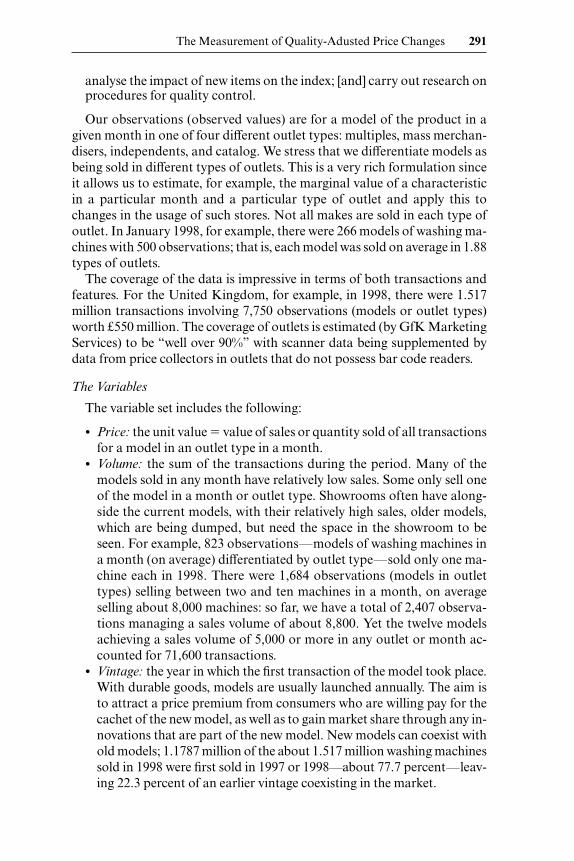
The results for the linear form are given in table 9.2. The coefficients werealmost invariably statistically significant with appropriate signs and magni-tudes. An additional spin speed of one rpm, for example, had a price pre-mium of £0.30. Between December and January, other quality characteris-tics held constant and prices fell from the mean of £405.71 by £25.33, to£380.38—that is, a fall of 6.2 percent. There was some evidence of hetero-skedasticity with the Breusch-Pagan test statistics of 27.7 and 9.0 for the lin-ear and semilog forms respectively, both exceeding the critical value of Chi-squared (3 degrees of freedom) � 7.815. However, the estimator remainsunbiased, and the standard errors were adjusted to be heteroskedastic-consistent using a procedure by White (1980).

The regressions were estimated on a data set that excluded models withsales of thirty or less in any month and a minimal number of models withextreme prices arising from variables not included in the data, such as stain-less steel washing machines. A failing of the dummy variable approach isthat models with only one transaction are given the same importance in theregression as a model with, say, 10,000 transactions. The choice of thirtywas based on some experimentation. The loss in the number of observa-tions was quite severe for washing machines from 7,750 to 3,600, whereasthe loss in terms of the volume of sales was minimal, from 1.517 million to1.482 million. An alternative approach is to use a sales volume weightedleast squares estimator, as considered later.

Exact (and Superlative) Hedonic Indexes

First, it is necessary to decide which quality-related variables are used inthe aggregation in equation (6a) and which for the adjustment in equation


4. With this approach a variable Z is transformed to (Z – 1)/. Since the limit of this as approaches zero is log Z, it is defined to be log Z when � 0. If all variables in a linear func-tional form are transformed in this way and then is estimated (in conjunction with the otherparameters) via a maximum likelihood technique, significance tests can be performed on tocheck for special cases. If � 0, for example, the functional form becomes Cobb-Douglas innature; if � 1 it is linear. A confidence interval on can be used to test whether or not it en-compasses 0 or 1.

5. The Bera-McAleer test involves obtaining predicted values log (z) and (z) from a semi-logarithmic and a linear formulation, respectively. Artificial regressions are then computed us-ing exp{log (z)} and log(z) on the left-hand-side, and the residuals from each of these regres-sions, v1 and v0 , are included in a further set of artificial regressions: log(z) � �0 � �1X1 � �0v1

� ε1; z � �0 � �1X1 � �1v0 � ε2. Using t-tests, if �0 is accepted we choose the log-linear model,and if �1 is accepted we choose the linear model, the test being inconclusive if both are rejectedor both accepted.

Table 9.2 Regression Results for Linear Hedonic Equation for 1998 (dependent variable: price)

Variable Estimated Coefficient Standard Error

C –981.290*** 115.562Months (benchmark: January)

February –0.214244 5.64587March 6.71874 5.37602April 0.220101 5.36765May –1.60710 5.37089June –5.02523 5.2291July –10.9314* 5.2195August –10.6569* 5.2936September –15.6103** 5.2193October –16.2413** 5.2970November –17.9056*** 5.3397December –25.3343*** 5.3068

CharacteristicsHeight (cm) –0.347469 0.291905Depth (cm) 6.12143*** 0.47413Width (cm) 6.26849*** 0.69974Water consumption (liters) –1.14070*** 0.06825Load capacity (kg) –0.287457** 0.096536Spin speed (rpm) 0.304251*** 0.006965Drying capacity—washer/dryer (kg) –0.335703 0.368737Condensor—washer/dryer 35.9352*** 6.2530Energy consumption (kWh per cycle) 0.331592** 0.104301Vintage 4.24294*** 0.90397

Type of machine (benchmark: front loader washing machine)

Top loader 228.876*** 12.125Twin tub –704.998*** 20.251Washer/dryer 64.6312*** 9.1877Washing machine with computer 127.455*** 8.856Washer/dryer with computer 129.682*** 16.406

Installation (benchmark: free-standing)Built-under integrated 238.908*** 10.1389Built-under –61.3298 42.8550Built-in integrated 293.221*** 27.349

Outlet type (benchmark: multiples)Mass merchandisers 23.1155*** 2.9010Independents 31.2458*** 2.5882Catalogs 71.8786*** 3.3023

Makes (benchmark: Bosch)AEG 66.8428*** 6.1338Siemens 46.9125*** 7.2096Hoover –68.0069*** 3.65656Miele 165.895*** 10.316Candy –98.8340*** 6.0759English Electric 7.99810*** 0.82048Ariston –21.9183* 8.5417New Pol –113.529 60.062

(6b). The �t estimates are then derived from monthly hedonic regressionsand multiplied by changes in the sales-weighted change in the mix of qual-ity characteristics to provide an adjustment to average prices ( p�) for use inthe main body of equation (6a).

The � coefficient is required for each K quality-related variable in equa-tion (6b) in each month. The specification of the regression equations esti-mated for this purpose used all variables, to avoid omitted variable bias,with only the relevant �t coefficient being used to generate ppp�. The specifica-tions were therefore similar to the time dummy variable method except thatseparate regressions were estimated for each month.6

A weighted least squares estimator was used, the weights being the vol-ume of sales. The mean R�2 over the twelve monthly hedonic regressions was0.842.7 The coefficients were almost invariably statistically significant and


Table 9.2 (continued)

Variable Estimated Coefficient Standard Error

Beko –134.695*** 10.558Zanussi 5.16116 4.12916Electro 0.7362 11.8086Indesit –68.7762*** 5.4285Neff 109.284*** 16.897Philco –108.286*** 25.939Ignis –22.4469*** 22.9162Creda –67.3200*** 7.4762Tricity/Bendi –58.2687*** 6.1059Hotpoint –32.5816*** 3.9348Servis –76.1764*** 5.7801Asko 164.781** 60.226

Na 3,600Mean of price 405.713Standard error of regression 59.8572Adjusted R2 0.8299Breusch-Pagan 27.7F-statistic (zero slopes) 314.626

aVolume of sales greater than thirty in a month or outlet type.***Statistically significant at the 0.1 percent level for two-tailed t-tests.**Statistically significant at the 1 percent level for two-tailed t-tests.*Statistically significant at the 5 percent level for two-tailed t-tests.

6. It is noted that observations with sales of 30 and less were not used for estimating the in-dividual coefficients, but all the data were used for the average prices, quantities, values, andsales-weighted mix of qualities in formulas.

7. Test statistics here are illustrative, being based on semilog and linear models for the dataas a whole, although they are indicative of the results for individual months (available from theauthors). Estimates for log-log models were not feasible, given the large number of dummyvariables on the right-hand side of the equation.

of reasonable magnitude with the appropriate sign.8 As with the dummyvariable method, the regressions were estimated using the linear and semi-log forms. The coefficients from the linear form were used to derive quality-adjusted prices for use in an arithmetic framework—that is, for Laspeyres,Paasche, and (superlative) Fisher hedonic indexes (equation [4]). The co-efficients from the semilog form were used to calculate base and current pe-riod weighted geometric means and (superlative) Törnqvist exact hedonicindexes given in footnote 1 and available from the authors. It is noted thatthe estimation of semilogarithmic functions as transformed linear regres-sions requires an adjustment to provide minimum variance unbiased esti-mates of parameters of the conditional mean. This involved the standard er-rors, which in any event were very small, although the adjustments wereundertaken (Goldberger 1968).

As explained in section 9.2, the exact hedonic approach has the advan-tage over matching of minimal loss of data. However, the more variables in-cluded in the aggregation in equation (6a), the greater the information loss,as either p�it–1 or p�it becomes unavailable in any period for comparison. In thelimiting case of all variables being included, the method collapses to thematched approach. If we aggregate over makes, or even makes and outlettypes, there is very little loss of data in terms of the number of observationsand volume of sales. Aggregating only over the 21 makes leaves 99.67 per-cent of observations and 99.97 percent of sales volume. Extending the ag-gregation to the 21 makes and 4 outlets, 84 combinations still has little lossof data—99.08 percent of observations and 99.92 percent of sales volume.Any manufacturer operating in a particular outlet type continues to do soon a monthly basis. Extending the aggregation further to 24 spin speeds(i.e., over 2,016 combinations) reduces the coverage to 95.9 percent of ob-servations and 99.6 percent of sales volume.

Matching

The matching procedure used incurred further loss of data: Only 83 per-cent of observations were used, although the missing ones were models inoutlets that were being discarded with low sales, the volume of sales used inthe matching being 97.8 percent.

The extent of the matching is illustrated for washing machines in 1998 intable 9.3. There were for example, 429 matched comparisons of a particularmodel in a specific outlet type in February 1998. These were selected from500 and 488 observations available in February and January 1998, respec-tively. In total there were 6,020 matched comparisons for 1998, which com-pares with 7,750 available in 1998 or, more fairly, 7,750 – 500 � 7,256 to ex-clude the January figures because the matched comparisons are over elevenmonthly comparisons as opposed to twelve months’ data.


8. Results are available from the authors.

This difference of 1,236 observations is price data that exist in either pe-riod t or period t � 1 but do not have a counterpart to enable a compari-son.9 Since they are models just born or about to die, they should have lowsales, and thus their omission should not unduly affect the index.10 The to-tal sales volume of matched comparisons was 1.3605 million, comparedwith 1.3906 million (unmatched but excluding January)—a difference ofabout 30,000 sales or about 2 percent of sales. From table 9.3 the monthlyvariation can be deduced. The worst loss of information was in the Marchto February comparisons: from (111.4 � 134.0)/2 � 122.7 thousand to118.6 thousand—a loss of 3.3 percent. For the September to October andOctober to November comparisons the losses were less than 1 percent. Aunit value index is given by

(7) � � � � �,

which is a weighted measure of price changes not adjusted for changes in thequality mix. It is included in the analysis for comparison.

∑pt�1xt�1��

∑xt�1

∑ ptxt�∑xt


Table 9.3 Data on Matching for Washing Machines, 1998

Number of Observations Volume of Sales (thousands)

Matched Unmatched Matched Unmatched Matched

January 500 126.2February 488 429 111.4 115.1March 605 425 134.0 118.6April 625 510 113.3 120.7May 647 527 112.5 111.3June 711 555 137.1 122.5July 744 620 116.3 124.9August 711 627 123.0 118.3September 717 606 150.4 135.1October 695 602 129.2 138.5November 643 566 124.8 125.8December 664 553 138.6 129.8

Note: Matched comparisons are between each month and the preceding one for chained in-dexes. There were, for example, 429 matched comparisons between February and January 1998taken from 488 observations (model in a specific outlet type) in February and 500 in January1998. Similarly, there were 425 matched comparisons between March and February 1998. Al-though the number of matched observations will not exceed those unmatched, the volume ofsales may do so.

9. If, for example, the matched item had sales in period t of 100 and in period t � 1 of 50,and a new model was launched in period t � 1 with sales of 10, the matched volume would be150/2 � 75 and the unmatched 60 in period t � 1.

10. The data are transactions over the month, so recently born or dead models may onlyhave been available for part of the month in question and have relatively low sales.

9.4 Results on the Three Methods for Scanner Data

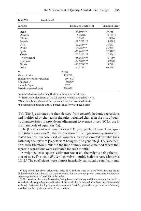
Table 9.4 and figure 9.1 provide results using the matched approach forseveral different formulas.

First, the Laspeyres and Paasche provide outer upper and lower bounds,respectively, to the superlative Fisher index, the extent of the substitutionbeing about 1.35 percent over the year, as consumers substituted away frommachines with relatively high price increases. Note that because these in-dexes are chained on a monthly basis, they are different from those thatarise from their fixed-base index counterparts. They allow the basket to beupdated each month, the substitution in each month being compoundedover the year. Second, figure 9.1 and table 9.4 show the unit value index, de-fined by index equation (7), to be unaffected by changes in the quality mixof models. Although the index shows only a slight overall fall in prices over


Table 9.4 Matched Quality-Adjusted Price Indexes by Formulas

Laspeyres Paasche Fisher Unit Values

January 100 100 100 100February 99.49 99.02 99.25 98.96March 99.52 98.77 99.15 100.61April 98.82 98.08 98.45 101.86May 97.91 97.05 97.48 102.04June 96.46 95.13 95.79 100.09July 95.78 94.21 94.99 101.86August 94.97 92.89 93.92 101.28September 94.24 91.95 93.09 100.28October 94.06 91.71 92.88 101.67November 93.39 90.70 92.03 99.89December 92.06 89.34 90.69 98.93

Fig. 9.1 Washing machines: Alternative formulas

the year of about 1 percent, and increases in other months compared withJanuary 1998, quality-adjusted price changes have fallen by just under 10percent over the year. The superlative matched index effectively adjusts forchanges in the quality mix of purchases being based on computationalmatching as opposed to statistical models. Finally, not reported here butavailable from the authors, the results for the superlative Törnqvist index infootnote 1 are similar to those for the superlative Fisher, the Törnqvist inDecember being 90.711, compared to Fisher’s 90.69. The geometric baseand current-period weighted indexes can be seen in footnote 1 to be ex-pected to be upper and lower inner bounds, respectively, on the superlativeindex because they incorporate some substitution effect (Shapiro andWilcox 1997)—again, results are available from the authors. All of this is aspredicted by economic theory. These indexes are the results of matchedcomputations with different weighting systems. The matching, however,loses 2 percent of the data by sales volume. We consider below exact (andsuperlative) hedonic indexes, which lose only 0.4 percent of sales volume.

Figure 9.2 and table 9.5 provide results for different approaches to meas-uring quality-adjusted price indexes using an arithmetic formulation. Theestimates from a linear model using the time dummy variable approachshow a fall of only 6.0 percent, falling, in December, outside the Laspeyresand (what would be) Paasche bounds of the matched and exact approaches.In section 9.3 we found the hedonic regression to have a relatively high R�2

with signs and values of the coefficients being as expected on a priorigrounds. The linear formulation was supported by a Box-Cox test, al-though the results from a semilog formulation are very similar, the indexfalling to 93.85—by 6.15 percent. By conventional standards, these esti-mates are quite acceptable. The difference between the results from otherapproaches is more likely to be a result of the absence of a weighting systemfor the time dummy variable approach. If prices of more popular models arefalling faster than those of unpopular ones, the weighted matched and ex-act approaches will take this into account, whereas the time dummy vari-able method will not. The concern here is with the time dummy variable ap-proach as it is usually employed. However, a sales-weighted least squaresestimator should in principle bring these estimates closer to the exact hedo-nic and matched results, although in practice the ordinary least squares andweighted least squares results were quite similar, a fall of 6.0 percent and 5.5percent, respectively (and for semilog 6.0 percent and 5.7 percent, respec-tively). The results from the exact (and superlative) hedonic approach andmatched estimates are not too dissimilar, a difference of about 2.0 and 1.7percentage points for Laspeyres and Fisher over the year. In this case study,the loss of data for the matching, at about 2 percent by volume, was rela-tively low, giving confidence to the matched results.

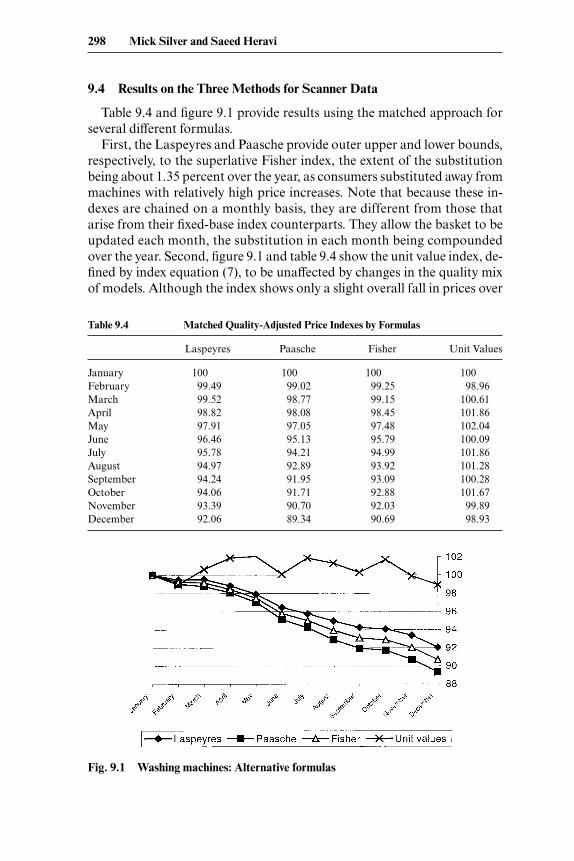
Finally, figure 9.3 shows the results for the exact (superlative) hedonic ap-proach at different levels of aggregation for Fisher indexes. As we expand


Fig

. 9.2

Qua

lity-

adju

sted

pri

ce in

dexe

s us

ing

arit

hmet

ic m

eans

the weighted price changes in the body of the formula in equation (6a) frommakes to makes within each outlet type, and then further by spin speed, theexact (superlative) hedonic index approaches the matched index.

In summary, this part of the paper uses scanner data to show how to mea-sure quality-adjusted price changes using scanner data. It casts doubt onthe use of the time dummy variable approach. It also argues for a matchedapproach as a special case of the theoretically based exact hedonic ap-proach, the matched approach being based on computational matching and


Table 9.5 Quality-Adjusted Price Indexes Based on Arithmetic Means

Exact Hedonic by Makeand Store Type Matched

Time Dummy Variable:Laspeyres Fisher Linear Laspeyres Fisher

January 100 100 100 100 100February 101.04 99.93 99.95 99.50 99.25March 101.26 100.23 101.59 99.52 99.15April 100.99 99.86 100.05 98.82 98.45May 100.25 99.11 99.62 97.91 97.48June 98.41 97.27 98.81 96.46 95.79July 98.19 97.02 97.41 95.78 94.99August 97.10 95.61 97.47 94.97 93.92September 96.96 95.24 96.30 94.24 93.09October 97.05 95.23 96.15 94.06 92.88November 96.14 94.18 95.76 93.39 92.03December 94.12 92.42 93.99 92.06 90.69

Fig. 9.3 Exact hedonic indexes at different levels of aggregation

not being subject to the ideosyncrasies of the econometric estimation of he-donic indexes (Griliches 1990; Triplett 1990). Caution is, however, advisedwhen the loss of data in matching is severe. In such a case an empirical in-vestigation into the trade-off between including variables in the aggregationand the resulting loss of data is advised.

9.5 Quality Adjustment and Consumer Price Index Practice:An Experiment

9.5.1 Alternative Methods

The above account concerned the measurement of quality-adjusted pricechanges using scanner data. However, the problems of quality adjustmentfor the practical compilations of CPIs by statistical offices are quite differ-ent. In general, display prices are recorded by price collectors on a monthlybasis for matched product varieties in a sample of individual stores. Whena variety is missing in a month, the replacement may be of a different qual-ity, and “like” may no longer be compared with “like.” Its quality-adjustedprice change has to be imputed by the statistical office. There is no problemof quality adjustment when varieties are matched. It is only when one is un-available and its price change has to be imputed that there is a problem. Thepurpose of this experiment is to attempt to replicate the practices used bystatistical offices in CPI compilation in order that the effects of differentquality adjustment techniques can be simulated.

It should be noted that this is not a trivial matter. Moulton, LaFleur, andMoses (1999) examined the extent to which price collectors were faced withunavailable varieties of TVs in the U.S. CPI. Between 1993 and 1997, 10,553prices on TVs were used, of which 1,614 (15 percent) were replacements, ofwhich, in turn, 680 (42 percent) were judged to be not directly comparable.Canadian experience for TVs over an almost identical period found 750 ofthe 10,050 (7.5 percent) to be replacements, of which 572 (76 percent) werejudged to be not directly comparable. For international price comparisonsthe problem is much more severe (Feenstra and Diewert 2000).

We should stress that sections 9.2–9.4 were concerned with how best tomeasure quality-adjusted price changes using scanner data. Here, the useof scanner data is to simulate CPI practices to help judge the veracity of al-ternative quality adjustment procedures that might be employed to sup-plement matched models procedures. A number of well-documented op-tions are available and are outlined in Turvey (1989); Reinsdorf, Liegey,and Stewart (1995); Moulton and Moses (1997); Armknecht, Lane, andStewart (1997); Armknecht and Maitland-Smith (1999); and Moulton,LaFleur, and Moses (1999), although the terminology differs; these op-tions include


• Imputation. Where no information is available to allow reasonable es-timates to be made of the effect on price of a quality change, the pricechange in the elementary aggregate group as a whole, to which the va-riety belongs, is assumed to be the same as that for the variety.

• Direct comparison. If another variety is directly comparable, that is, ifit is so similar it can be assumed to have the same base price, its pricereplaces the missing price. Any difference in price level between thenew and old is assumed to be due to price changes and not qualitydifferences.

• Direct quality adjustment. Where there is a substantial difference in thequality of the missing and replacement varieties, estimates of the qual-ity differences are made to enable quality-adjusted price comparisonsto be made.

For illustration, consider a product variety with a price of £100 in Janu-ary. In October, a replacement version with a widget attached is priced at£115. The direct comparison would use the price of an essentially identicalvariety. The direct quality adjustment method requires an estimate of theworth of the widget. For example, if it was found that the widget increasedthe product’s flow of services by 5 percent, the £115 in October could becompared with an adjusted base-period price of £100 (1.05) � £105. Theimputation approach would use the index for the relevant product group. Ifthis was 110.0 in October (January � 100.0), the replacement item wouldhave a revised base-period price of £115/1.10 � £104.55 to compare withthe new price of £115;that is, 115/104.55 × 100 � 110.0, a 10 percent in-crease in price, the residual 5 percent being assumed to be due to qualitydifferences.

Moulton, LaFleur, and Moses (1999) note that the direct or explicit qual-ity adjustment approach can be used with data from manufacturers on thecost of quality changes or coefficients from hedonic regressions as explicitestimates of quality differences. Valuable insights into the validity of suchmethods can be gained by using a number of such methods on actual CPIdata and comparing the results; seminal work in this area includes Lowe(1999) and Moulton, LaFleur, and Moses (1999). The alternative approachadopted here is to attempt to replicate such procedures using scanner data.

9.5.2 The Experiment

The purpose of this experiment is to replicate CPI data collection usingscanner data to provide a means by which different CPI procedures can beemulated. The formulation here is relatively crude, being an initial attemptat the exercise. However, we hope it will be useful for illustrative purposes.The data are the same monthly data on washing machines in 1998 used insections 9.3 and 9.4. We start by taking a January fixed basket of washing


machines comprising all varieties for which there was a transaction in Jan-uary. Our varieties are for a model in one of four outlet types: multiples,mass merchandisers, catalogs, and independents. Since many models areonly sold in chains of particular outlets, the classification is in practicecloser to a given model in a specific chain or even individual outlet, whichis the price observed by a price collector. The unit value of each variety inJanuary is treated as the average display price collected by the price collec-tors. Since the volume of transactions is known for each variety, the Janu-ary sample is taken to be the universe of every transaction of each variety.This January universe is the base-period active sample. We can, of course,subsequently modify this by using different sampling procedures and iden-tify their effects on the index.

If the variety in each outlet type continues to exist over the remainingmonths of the year, matched comparisons are undertaken between the Jan-uary prices and their counterparts in successive months. Consider again forillustration table 9.1, the case of four varieties existing in January, each withrelative expenditures of w1, w2, w5, and w6 and prices of p11, p21, p51, and p61. ALaspeyres price index for February compared with January � 100.0 isstraightforward. In March the prices for varieties 2 and 6 are missing. Eachof these was collected from different outlet types, multiples and mass mer-chandisers in this example. To enable Laspeyres price comparisons to beundertaken in such instances, a range of methods was utilized for the scan-ner data, including the following:

1. Implicit imputation. Price comparisons were only used when Januaryprices could be matched with the month in question. In our example theJanuary to March comparisons were based on varieties 1 and 5 only, theprice changes of varieties 2 and 6 being assumed to be the same as these re-maining varieties. The weights for varieties 1 and 5 would be w1/(w1 � w5)and w5 /(w1 � w5), respectively.

2. Targeted implicit imputation. The price changes of missing varietiesfor a specific make within an outlet type were assumed to be the same as forthe remaining active sample for that make within its outlet type. If we as-sumed varieties 1 and 2 and 5 and 6 are of the same make, then the weightsfor varieties 1 and 5 would be (w1 � w2) /W and (w5 � w6) /W, respectively,where W � (w1 � w2 � w5 � w6 ).

3. Direct comparison. Within each outlet type a search was made for thebest match first, by matching brand, then in turn by type (see earlier section“The Variables”), width, and spin speed. If more than one variety wasfound, the selection was according to the highest value of transactions (ex-penditure). In our example, varieties 3 or 4 and 7 would, respectively, replacevarieties 2 and 6 in March.

4. Explicit hedonic: predicted versus actual. A hedonic regression of the


(log of the) price of model i in period t on its characteristics set ztki was esti-mated for each month, given by

(8) ln pti � �0t � ∑K

k�1

�ktzkit � εit.

Say the price of variety m goes missing in March, period t � 2. The price ofvariety m can be predicted for March if we insert the characteristics of vari-ety m into the estimated regression equation for March and similarly forsuccessive months. The predicted price for this “old” unavailable variety min March and its price comparison with January (period t) are respectivelygiven by

(9) pm,t�2 � exp��0,t�2 �∑�k,t�2zk,m� for �p

p

ˆm

m

,t�

,t

2� � old

The “old” denotes that the comparison is based on a prediction of theprice of the unavailable variety in the current period rather than the (new)replacement variety’s price in the base period. In our example we would es-timate p23, p24, and so on, and p63, p64, and so on, and compare them with p21

and p61, respectively. We would effectively fill in the blanks for varieties 2and 6.

An alternative procedure is to select for each missing m variety a re-placement n variety using the routine described in step (3) above. In thiscase the price of n in period t � 2, for example, is known, and we require apredicted price for n in period t. The predicted price for the “new” varietyand required price comparison are

(10) pn,t � exp��0,t � ∑�k,t zk,n� for �pn

p,t

ˆn

�

,t

2� � new,

that is, the characteristics of variety n are inserted into the right-hand sideof an estimated regression for period t. The price comparisons of equation(9) would be weighted by wm,t , as would those of its replaced price compar-ison in equation (10).

A final alternative is to take the geometric mean of the formulations inequations (9) and (10) on grounds akin to those discussed by Diewert (1997)for similar index number issues.

5. Explicit hedonic: predicted versus predicted. A further approach wasthe use of predicted values for, say, variety n in both periods, for example,pn,t�2 /pn,t. Consider a misspecification problem in the hedonic equation. Forexample, there may be an interaction effect between a brand dummy and acharacteristic—say, a Sony television set and Nicam stereo sound. Posses-sion of both characteristics may be worth 5 percent more on price (from asemilogarithmic form) than their separate individual components (for evi-dence of interaction effects, see Curry, Morgan, and Silver 2001). The use of


pn,t�2 /pn,t would be misleading since the actual price in the numerator wouldincorporate the 5 percent premium, whereas the one predicted from astraightforward semilogarithmic form would not. A more realistic ap-proach to this issue might be to use predicted values for both periods. Westress that in adopting this approach we are substituting for a recorded, ac-tual price an imputation. This is not desirable, but neither would be theform of bias discussed above.

The comparisons using predicted values in both periods are given as

(11) �p

pn,t

ˆn

�

,t

2� for the “new” variety

�p

p

ˆm,

ˆm

t�

,t

2� for the disappearing or “old” variety, or

�� p

p

ˆn,t

ˆn

�

,t

2��

p

p

ˆm,

ˆm

t�

,t

2��0.5

as a (geometric) mean of the two.6. Explicit hedonic: adjustments using coefficients. In this approach, a re-

placement variety was found using the routine in step (3) above and anydifferences between the characteristics of the replacement n in, for example,t � 2 and m in period t ascertained. A predicted price for n in period t, thatis, pn,t, was determined and compared with the actual pn,t�2. However, unlikethe formulation in equation (10), pn,t was estimated by applying the subset ofthe k characteristics that distinguished m from n to their respective marginalvalues in period t estimated from the hedonic regression and adjusting theprice of pm,t . For our illustration, if the nearest replacement for variety 2 wasvariety 3, then the characteristics that differentiate variety 3 from variety 2were identified, and the price in the base period, p31 is estimated by adjust-ing p21 using the appropriate coefficients from the hedonic regression in thatmonth. For example, if variety 2 had an 800 rpm spin speed and variety 3 a1,100 rpm spin speed, other things being equal, the marginal value of the300 rpm differential would be estimated from the hedonic regression, andp21 would be adjusted for comparison with p33. Note that if the z variables inthe characteristic set are orthogonal to each other the results from this ap-proach will be identical to those from equation (10). A similar approach toequation (9) was also undertaken that only used the salient distinguishingcharacteristics and the geometric mean of the two calculated. These sixmethods provide in all twelve different measures of quality-adjusted pricechanges.

9.5.3 The Study

Table 9.6 provides a summary of the data used. In January 1998 there were500 varieties (models in one of the four outlet types—multiples, mass mer-chandisers, catalogs, and independents) of washing machines accounting


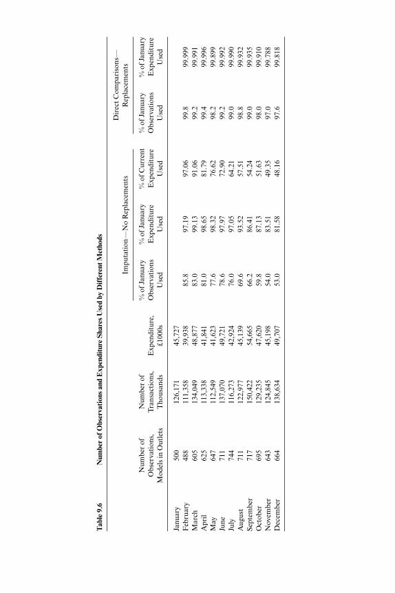
Tab

le 9

.6N

umbe

r of

Obs

erva

tion

s an

d E

xpen

ditu

re S

hare

s U

sed

by D

iffe

rent

Met

hods

Dir

ect C

ompa

riso

ns—

Rep

lace

men

tsIm

puta

tion

—N

o R

epla

cem

ents

Num

ber

ofN

umbe

r of

%

of J

anua

ry%

of J

anua

ry%

of C

urre

nt%

of J

anua

ry%

of J

anua

ryO

bser

vati

ons,

Tra

nsac

tion

s,E

xpen

ditu

re,

Obs

erva

tion

sE

xpen

ditu

reE

xpen

ditu

reO

bser

vati

ons

Exp

endi

ture

Mod

els

in O

utle

tsT

hous

ands

£100

0sU

sed

Use

dU

sed

Use

dU

sed

Janu

ary

500

126,

171

45,7

27F

ebru

ary

488

111,

358

39,9

3885

.897

.19

97.0

699

.899

.999

Mar

ch60

513

4,04

948

,877

83.0

99.1

391

.06

99.2

99.9

91A

pril

625

113,

338

41,8

4181

.098

.65

81.7

999

.499

.996

May

647

112,

549

41,6

2377

.698

.32

76.6

298

.299

.899

June

711

137,

070

49,7

2178

.697

.97

72.9

099

.299

.992

July

744

116,

273

42,9

2476

.097

.05

64.2

199

.099

.990

Aug

ust

711

122,

977

45,1

3969

.693

.52

57.5

198

.899

.932

Sept

embe

r71

715

0,42

254

,665

66.2

86.4

154

.24

99.0

99.9

35O

ctob

er69

512

9,23

547

,620

59.8

87.1

351

.63

98.0

99.9

10N

ovem

ber

643

124,

845

45,1

9854

.083

.51

49.3

597

.099

.788

Dec

embe

r66

413

8,63

449

,707

53.0

81.5

848

.16

97.6

99.8

18

for 126,171 transactions. The distribution was highly skewed, with the top 5percent and 10 percent of varieties (in an outlet type) accounting for 49 per-cent and 66 percent of transactions, respectively, in January. The indexes inthis section are fixed-base January 1998 � 100.0 indexes compiled over theperiod January to December 1998. Unlike the chained indexes considered inprevious sections, they take no account of varieties introduced after Januaryunless they replace a variety that is “missing”—that is, it no longer has anytransactions. The imputation approach does not replace missing varieties.Table 9.6 shows that by December, only 53 percent of the January basket ofvarieties were used for the December/January index, although these ac-counted for 81.6 percent of January expenditure. Varieties with lower salesvalues dropped out more quickly. However, the remaining 0.53 (500) � 265varieties in December only accounted for 48.2 percent of the value of trans-actions in December. The active sample relating to the universe of transac-tions in December had deteriorated, and although they are not part of thiscurrent study, insights into the nature of the deterioration can be ascer-tained from the experiment. For example, this type of experiment could beused to consider the effects of renewing the item selection more frequently.The fall in the coverage of the active sample is mitigated by the introductionof replacements when using direct comparisons. The weights used remain,of course, those in January 1998. However, the sample of information usedin successive months draws on the replacement varieties.

The search procedure outlined above for replacements for direct com-parisons, and used in some of the hedonic methods, had a minimum condi-tion—that the replacement must at least be of the same make in a given out-let type. This can be seen from table 9.6 to have been generally met, thefall-off being negligible. The hedonic approach benefited from use of infor-mation on the whole sample in each month for the estimation of the equa-tions. The estimated regression equations were based on the whole samplein spite of the inclusion of varieties with limited transactions on the groundsthat such varieties were more likely to be the ones going missing. The twelveregressions estimated in each month had a mean R�2 of 0.80, and in each casethe null hypothesis of the individual coefficients being jointly equal to zerowas rejected by an F-test. The average monthly sample size was 558.

9.5.4 The Results

Table 9.7 provides the results. The extent of any bias arising from the im-putation approach is dictated by the ratio of missing price comparisons to thetotal number of comparisons and by the difference between quality-adjustedprice changes of the missing varieties, had they continued to exist, and thoseof other varieties (see the appendix). The bias from the class mean imputa-tion approach should be smaller than the imputation approach, and thesemethods show the choice between the results matters—an approximately 2percentage point difference over the year, for a roughly 10 percent fall.


Tab

le 9

.7L

aspe

yres

Ind

exes

Pre

dict

ed v

ersu

s A

ctua

lA

djus

tmen

t via

Coe

ffici

ents

Pre

dict

ed v

ersu

s P

redi

cted

Tar

gete

dD

irec

tG

eom

etri

cG

eom

etri

cG

eom

etri

cIm

puta

tion

Impu

tati

onC

ompa

riso

nO

ldN

ewM

ean

Old

New

Mea

nO

ldN

ewM

ean

Janu

ary

100.

0010

0.00

100.

0010

0.00

100.

0010

0.00

100.

0010

0.00

100.

0010

0.00

100.

0010

0.00

Feb

ruar

y99

.49

99.5

099

.30

99.7

599

.16

99.4

599

.41

99.3

899

.40

99.4

999

.48

99.4

9M

arch

99.2

999

.29

99.2

699

.35

99.1

799

.25

99.2

399

.20

99.2

299

.27

99.2

999

.28

Apr

il98

.30

98.2

998

.45

98.2

398

.29

98.2

598

.21

98.3

898

.30

98.0

998

.31

98.2

0M

ay97

.06

98.8

997

.30

96.9

597

.10

97.0

296

.94

97.1

897

.06

96.7

597

.09

96.9

2Ju

ne94

.98

94.9

795

.09

95.0

094

.95

94.9

894

.92

95.0

594

.98

94.9

195

.07

94.9

9Ju

ly93

.14

92.9

793

.13

93.4

493

.08

93.2

693

.28

93.1

093

.19

93.4

093

.22

93.3

1A

ugus

t93

.64

92.6

294

.49

94.6

493

.83

94.2

494

.28

94.0

794

.18

94.0

993

.87

93.9

8Se

ptem

ber

93.5

592

.01

94.0

394

.91

92.2

693

.58

93.3

793

.29

93.3

394

.06

93.9

694

.01

Oct

ober

91.8

490

.74

91.7

592

.99

90.4

891

.73

91.4

991

.30

91.4

092

.13

92.1

492

.13

Nov

embe

r91

.52

90.2

091

.47

93.2

689

.94

91.5

990

.85

90.8

390

.84

91.7

592

.17

91.9

6D

ecem

ber

90.8

788

.94

91.8

192

.74

90.0

991

.41

91.2

691

.19

91.2

391

.63

91.6

691

.55

The price fall measured using direct comparisons was found to be smallerthan the class mean result—a fall of 8.2 percent compared with 11.1 per-cent. A priori there is no expectation of the direction of bias from the tar-geted imputation approach (see the appendix), although for direct compar-isons the replacements in varieties are more likely to be priced higher thanthe missing ones, the smaller fall in price thus being expected. However,given that the selection of replacement is not governed by the judicious se-lection of price collectors but by a computational procedure, the extent ofthe difference is smaller than expected.

The use of hedonic adjustment methods provides an explicit basis for thequality adjustments. The results for the predicted versus actual have a smallerfall for the “old” (equation [9]) than “new” (equation [10]) comparison (table9.7). The actual old, disappearing varieties could be argued to be more likelyto be below the hedonic surface as they price to clear the market, whereas theactual new varieties are more likely to be above the hedonic surface as theyprice-skim segments of consumers with higher price elasticities. However, theeffect of both is to increase the price change. The geometric mean of an 8.6percent fall is slightly higher than the other results, as expected.

The above estimates were also undertaken using a subset of the regressioncoefficients applied only to the characteristic differences that took place. Ifthe variables for the characteristics are orthogonal to each other, the resultswill be the same as those for equations (9) and (10) discussed above. The ad-justments are affected by multicollinearity as imprecise estimates of indi-vidual marginal values are utilized for the adjustment. Multicollinearity oc-curs when characteristics are bundled together, and it is not clear whetherthe differences between the results of the two formulations are some mea-sure of this. Nonetheless, the results for the two geometric means are quitesimilar—a fall of 8.8 percent for the adjustment via coefficients.

The final set of estimates is the predicted versus predicted. The old andnew estimates are very close, with a geometric mean and a fall of 8.4 per-cent. This compares with the geometric mean of the predicted versus actualof 8.6 percent, implying that the results, when averaged using the geometricmean, are not subject to serious misspecification error.

Thus, in summary, different hedonic adjustment techniques provide sim-ilar results, although the old and new predicted to actual appear to workbest as a geometric mean. This similarity is encouraging, given the plethoraof such approaches. These results are also similar to those from a computa-tional, direct replacement method, but both imputation approaches lead tolarger falls in prices, a result with no immediate explanation, given the anal-ysis in the appendix.

9.5.5 Further Work

The results are exploratory in the sense that they arise from an experi-mental formulation that is subject to some limitations that cannot be easily


remedied as well as some restrictions that can. A major limitation is that theobservations are for a product variety in a specific outlet type, as opposedto in a specific outlet (in a geographical place). That some models are spe-cific to some outlet chains helps, but we cannot distinguish here between thelocations of the outlets, although in principle this is possible with scannerdata. This in itself may not be problematic for price comparisons, sincethere is still some debate over the validity of using the aggregated unit val-ues over outlets for price comparisons (Balk 1999; Diewert 1990; de Haanand Opperdoes 1998). However, the concept of “missing” prices used hereis not appropriate since a price collector may, for example, find a price miss-ing for a variety in an outlet in Cardiff while other price collectors may findprice quotes for the same variety in different stores or locations. The exper-iment would only treat prices as missing if there were no transactions any-where for the product variety. Scanner data provide a proxy variable on theextent to which each variety is sold in different outlets, and use of this is be-ing considered to develop the experiment.

Further work might also include consideration of the effects of the fol-lowing:

• different sampling schemes for the January selection as opposed to theuse of the universe of transactions

• more frequent item selection (rebasing) on the need for quality adjust-ments

• more frequent item selection (rebasing) on the coverage of the universeof transactions

• variations in the specification and sample used for the hedonic regres-sions

• different selection criteria for replacements• use of different formulas• comparison with hedonic indexes• different rules for deciding when a variety is “missing”• more refined class imputation procedures• missing market innovations• extension to other products

Appendix

Triplett (2001) in a draft OECD manual has been responsible for a detailedanalysis of the implicit bias from imputations, and although the formula-tion here is quite different, there is much that has been usefully applied fromhis analysis. For i � 1 . . . m varieties where Pm,t is the price of variety m in


period t, Pn,t�1 is the price of a replacement variety n in period t � 1, A(h) isa quality adjustment to Pn,t�1 that equates its quality services to Pm,t�1 suchthat the quality-adjusted price P∗

m,t�1 � A(h)Pn,t�1, and Q is the implicit ad-justment that allows the method to work, the arithmetic formulation forone missing variety is given by

(A1) �m

1��

P

P

∗m

m

,t

,

�

t

1� � ∑

m�1

i�1

�P

Pi,t

i,

�

t

1�� (m �

1

1)�∑

m�1

i�1

�P

Pi,t

i,

�

t

1�� Q

(A2) Q � �m

1� �

P

P

∗m

m

,t

,

�

t

1� � �

m(m

1

� 1)� ∑

m�1

i�1

�P

Pi,t

i

�

,t

1�

and for x missing varieties by

(A3) Q � �m

1�∑

x

i�1

�P

P

∗m

m

,t

,

�

t

1� � �

m(m

x

� x)� ∑

m�x

i�1

�P

Pi,t

i

�

,t

1�

The relationships are readily visualized if r1 is defined as the respectivegeometric or arithmetic mean of price changes of varieties that continue tobe recorded and r2 that of quality-adjusted missing varieties, that is, for thearithmetic case where

(A4) r1 � �∑m�x

i�1

�P

Pi,t

i,

�

t

1�� (m � x)

r2 � �∑x

i�1

�P

P

∗i,

i

t

,

�

t

1�� x

then the ratio of arithmetic mean biases from substituting equations (A4) in(A3) is

(A6) Qg � �m

x� (r2 � r1 ),

which equal zero when r1 � r2 . The bias depends on the ratio of missing val-ues and the difference between the mean of price changes for existing vari-eties and the mean of quality-adjusted replacement to missing pricechanges. Note that the bias is small if either (x/m) or the difference betweenr1 and r2 is small. Furthermore, note that the method is reliant on a com-parison between price changes for existing varieties and quality-adjustedprice changes for the replacement/missing comparison. This is more likelyto be justified than a comparison without the quality adjustment. For ex-ample, suppose we had m � 3 varieties, each with a price of 100 in period t.Let the t � 1 prices be 120 for two varieties, but assume the third is miss-ing—that is, x � 1—and is replaced by a variety with a price of 140, 20 ofwhich is due to quality differences. Then the arithmetic bias as given inequation (A6), where x � 1, m � 3 and r2 � [(A(h) � Pn,t�1) /Pm,t ], is


�1

3��140

10

�

0

20� � �

2

1

4

0

0

0

/2�� 0.

Had the bias depended on the unadjusted price of 140 compared with 100,the method would be prone to serious error. In this calculation the directionof the bias is given by (r2 – r1 ) and does not depend on whether quality is im-proving or deteriorating, that is, whether (A(h) � Pn,t�1 or A(h) � Pn,t�1. IfA(h) � Pn,t�1, a quality improvement, it is still possible that r2 � r1 and thatthe bias may be negative, a point stressed by Jack Triplett.

References

Abraham, K., J. Greenless, and B. Moulton. 1998. Working to improve the Con-sumer Price Index. Journal of Economic Perspectives 12 (1): 23–36.

Arguea, N. M., C. Haseo, and G. A. Taylor. 1994. Estimating consumer preferencesusing market data: An application to U.S. automobile demand. Journal of AppliedEconometrics 9:1–18.

Armknecht, P. A., W. F. Lane, and K. J. Stewart. 1997. New products and the U.S.Consumer Price Index. In The economic of new goods. Studies in Income andWealth, vol. 58, ed. T. F. Bresnaham and R. J. Gordon, 375–96. Chicago: Uni-versity of Chicago Press.

Armknecht, P. A., and F. Maitland-Smith. 1999. Price imputation and other tech-niques for dealing with missing observations, seasonality, and quality changes inprice indices. IMF Working Paper no. WP/99/78. Washington, D.C.: Interna-tional Monetary Fund, Statistics Department.

Astin, J. A., and D. J. Sellwood. 1998. Harmonization in the European Union: A re-view of some technical issues. Proceedings of the third meeting of the InternationalWorking Group on Price Indices, ed. B. Balk, 291–308. Research Paper no. 9806.Voorburg, the Netherlands: Statistics Netherlands.

Balk, B. 1999. On the use of unit value indices as consumer price sub-indices. In Pro-ceedings of the fourth International Working Group on Price Indices, ed. W. Lane,112–20. Washington, D.C.: Bureau of Labor Statistics.

Berndt, E. R., Z. Grilches, and N. J. Rappaport. 1995. Econometric estimates ofprice indices for personal computers in the 1990s. Journal of Econometrics68:243–68.

Blow, L., and I. Crawford. 1999. Cost of living indices and revealed preference. Lon-don: The Institute of Fiscal Studies.

Boskin, M. S., chairman. Advisory Commission to Study the Consumer Price In-dex. 1996. Towards a more accurate measure of the cost of living. Interim Reportto the Senate Finance Committee. Washington, D.C.

Boskin, M. S., E. R. Delberger, R. J. Gordon, Z. Griliches, and D. W. Jorgenson.1998. Consumer prices in the Consumer Price Index and the cost of living. Jour-nal of Economic Perspectives 12 (1): 3–26.

Bradley, R., B. Cook, S. G. Leaver, and B. R. Moulton. 1998. An overview of re-search on potential uses of scanner data in the U.S. CPI. Proceedings of the thirdmeeting of the International Working Group on Price Indices, ed. B. Balk, 169–182.Research Paper no. 9806. Statistics Netherlands.


Cameron, J., and A. Collins. 1997. Estimates of hedonic ageing for partner search.Kyklos 50 (3): 409–18.

Cole, R., Y. C. Chen, J. A. Barquin-Stolleman, E. Dulberger, N. Helvacian, and J.H. Hodge. 1986. Quality-adjusted price indexes for computer processors and se-lected peripheral equipment. Survey of Current Business 65 (1): 41–50.

Cunningham, A. 1996. Measurement bias in price indices: An application to theUK’s RPI. Bank of England Working Paper Series, no. 47. London: Bank of En-gland.

Curry, B., P. Morgan, and M. Silver. 2001. Hedonic regressions, misspecifications,and neural networks. Applied Economics 33:659–71.

Dalen, J. 1998. Experiments with Swedish scanner data. Proceedings of the thirdmeeting of the International Working Group on Price Indices, ed. B. Balk, 163–68.Research Paper no. 9806. Voorburg, the Netherlands: Statistics Netherlands.

Diewert, W. E. 1976. Exact and superlative index numbers, Journal of Econometrics4:115–45.

———. 1978. Superlative index numbers and consistency in aggregation. Econo-metrica 46:883–900.

———. 1980. Aggregation problems in the measurement of capital. In The mea-surement of capital, Studies in Income and Wealth, vol. 45, ed. Dan Usher, 433–528. Chicago: University of Chicago Press.

———. 1993. The early history of price index number research. In Essays in indexnumber theory, vol. 1, ed. W. E. Diewert and A. O. Nakamura, 33–65. Amster-dam: North Holland.

———. 1995. Axiomatic and economic approaches to elementary price indices.Discussion Paper no. 95-01. Vancouver, Canada: University of British Columbia,Department of Economics.

———. 1996. Sources of bias in consumer price indices. Discussion Paper no. DP-96-04. University of New South Wales, School of Economics.

———. 1997. Alternative strategies for aggregating prices in the CPI: Comment.Federal Reserve Bank of St Louis Review 79 (3): 113–25.

Feenstra, R. C. 1995. Exact hedonic price indices. Review of Economics and Statis-tics 77:634–54.

Feenstra, R. C., and E. W. Diewert. 2000. Imputation and price indices: Theory andevidence from the International Price Program. BLS Working Paper no. 335.Washington, D.C.: Bureau of Labor Statistics, Office of Prices and Living Con-ditions.

Fixler, D., and K. Zieschang. 1992. Incorporating ancillary measures of processesand quality change into a superlative productivity index. Journal of ProductivityAnalysis 2:245–67.

Forsyth, F. G., and R. F. Fowler. 1981. The theory and practice of chain price indexnumbers. Journal of the Royal Statistical Society, series A, 144 (2): 224–47.

Gandal, N. 1994. Hedonic price indices for spreadsheets and empirical test for net-work externalities. RAND Journal of Economics 25 (1): 160–70.

———. 1995. Competing compatibility standards and network externalities in thePC market. Review of Economics and Statistics 77:599–608.

Goldberger, A. A. 1968. The interpretation and estimation of Cobb-Douglas func-tions. Econometrica 35 (3–4): 464–72.

Gordon, R. L. 1990. The measurement of durable goods prices. Chicago: Universityof Chicago Press.

Griliches, Z. 1990. Hedonic price indices and the measurement of capital and pro-ductivity: Some historical reflections. In Fifty years of economic measurement:The Jubilee Conference of Research in Income and Wealth, Studies in Income and


Wealth, vol. 54, ed. E. R. Berndt and J. E. Triplett, 185–206. Chicago: Universityof Chicago Press.

Haan, J. de, and E. Opperdoes. 1998. Estimation of the coffee price index usingscanner data: The choice of the micro index. Proceedings of the third meeting ofthe International Working Group on Price Indices, ed. B. Balk, 191–202. ResearchPaper no. 9806. Voorburg, the Netherlands: Statistics Netherlands.

Hausman, J. R. 1997. Valuation of new goods under perfect and imperfect condi-tions. In The economics of new goods, Studies in Income and Wealth vol. 58, ed. T. Bresnahan and R. J. Gordon, 209–48. Chicago: University of Chicago Press.

Hawkes, W., and R. Smith. 1999. Improving consumer price measurements throughthe use of scanner data and market segmentation. In Proceedings of the Measure-ment of Inflation Conference, ed. M. Silver and D. Fenwick, 283–99. Cardiff,Wales: Cardiff Business School.

Hicks, J. R. 1940. The valuation of the social income. Economica 7:105–24.Hoffmann, J. 1998. Problems of inflation measurement in Germany. Economic Re-

search Group of Deutsche Bundesbank Discussion Paper no. 1/98. Frankfurt:Deutsche Bundesbank.

Ioannidis, C., and M. Silver. 1999. Estimating hedonic indices: An application toU.K. television sets. Zeitschrift fur Nationalokonomie (Journal of Economics) 69(1): 71–94.

Kmietowicz, Z. W., and M. S. Silver. 1980. New products and the Index of Indus-trial Production. Journal of Development Studies 16 (4): 463–67.

Kokoski, M., K. Waehrer, and P. Rozaklis. 1999. Using hedonic methods for qual-ity adjustment in the CPI: The consumer audio products component. BLS Work-ing Paper. Washington, D.C.: Bureau of Labor Statistics, Division of Price andIndex Number Research. Available at [http://www.bls.gov/cpi/cpiaudio.htm].

Konüs, A. A. 1939 (1924). The problem of the true index of the cost-of-living.Econometrica 7 (1): 10–29. First published in Russian.

Lerner, J. 1995. Pricing and financial resources: An analysis of the disk drive indus-try, 1980–88. The Review of Economics and Statistics 77:585–98.

Lowe, R. 1999. Televisions: Quality changes and scanner data. In Proceedings of thefourth meeting of the International Working Group on Price Indices, ed. W. Lane,5–20. Washington, D. C.: Bureau of Labor Statistics.

McFadden, D. 1983. Econometric models of probabilistic choice. In Structural anal-ysis of discrete data with econometric applications, ed. Charles F. Manski andDaniel McFadden, 198–272. Cambridge: MIT Press.

Mills, E. S., and R. Simenauer. 1996. New hedonic estimates of regional constantquality house prices. Journal of Urban Economics 39 (2): 209–15.

Moulton, B., T. J. LaFleur, and K. E. Moses. 1999. Research on improved qualityadjustments in the CPI: The case of televisions. In Proceedings of the fourth meet-ing of the International Working Group on Price Indices, ed. W. Lane, 77–99. Wash-ington, D.C.: Bureau of Labor Statistics.

Moulton, B., and K. E. Moses. 1997. Addressing the quality change issue in theConsumer Price Index. Brookings Papers on Economic Activity, issue no. 1:305–49.

Murray, J., and N. Sarantis. 1999. User cost, forward-looking behaviour, and the de-mand for cars in the U.K. Journal of Economics and Business 51 (3): 237–58.

Nelson, R. A., T. L. Tanguay, and C. D. Patterson. 1994. A quality-adjusted priceindex for personal computers. Journal of Business and Economics Statistics 12 (1):23–31.

Rasmussen, D. W., and T. W. Zuehlke. 1990. On the choice of functional form forhedonic price functions. Applied Economics 22 (4): 431–38.


Reinsdorf, M. 1996. Constructing basic components for the U.S. CPI from scannerdata: A test using data on coffee. Working Paper no. 277. Washington, D.C.: Bu-reau of Labor Statistics.

———. 1998. Divisia indices and the representative consumer problem. In Pro-ceedings of the fourth meeting of the International Working Group on Price Indices,ed. W. Lane, 210–235. Washington, D.C.: Bureau of Labor Statistics.

Reinsdorf, M., P. Liegey, and K. Stewart. 1995. New ways of handling qualitychange in the U.S. Consumer Price Index. Working Paper no. 276. Washington,D.C.: Bureau of Labor Statistics.

Rosen, S. 1974. Hedonic prices and implicit markets: Product differentiation andpure competition. Journal of Political Economy 82:34–49.

Saglio, A. 1995. Comparative changes in average price and a price index: Two casestudies. In Proceedings of the first meeting of the International Working Group onPrice Indices, ed. L. M. Duchare. Ottawa: Statistics Canada. Available at [http://www4.statcan.ca/secure/english/ottawagroup/toc1.htm].

Shapiro, M. D., and D. W. Wilcox. 1997. Alternative strategies for aggregating pricesin the CPI. Federal Reserve Bank Review 79 (3): 113–26.

Silver, M, 1995. Elementary aggregates, micro-indices, and scanner data: Some is-sues in the compilation of consumer prices. Review of Income and Wealth 41:427–38.

———. 1999. An evaluation of the use of hedonic regressions for basic componentsof consumer price indices. Review of Income and Wealth 45 (1): 41–56.

Stewart, K. G., and J. C. H. Jones. 1998. Hedonic and demand analysis: The implicitdemand for player attributes. Economic Inquiry 36 (2): 192–202.

Szulc, B. J. 1983. Linking price index numbers. In Price level measurement, ed. W. E.Diewert and C. Montmarquette, 537–66. Ottawa: Statistics Canada.

Triplett, J. E. 1987. Hedonic functions and hedonic indices. In The new Palgravesdictionary of economics. 630–34. Bastingstoke, England: Palgrave Macmillan.

———. 1990. Hedonic methods in statistical agency environments: An intellectualbiopsy. In Fifty years of economic measurement: The Jubilee Conference on Re-search in Income and Wealth, Studies in Income and Wealth, vol. 56, ed. E. R.Berndt and J. E Triplett, 207–38. Chicago: University of Chicago Press.

———. 2001. Draft of handbook on quality adjustment of price indexes for infor-mation and communication technology products. OECD Directorate for Sciencetechnology and Industry. Paris: Organization for Economic Cooperation and De-velopment.

Turvey, R. 1989. Consumer price indices. Geneva: International Labour Organisa-tion.

———. 1999a. Draft of elementary aggregate indices manual. Available at [http://www.turvey.demon.co.uk]. Revised April.

———. 1999b. Incorporating new models into a CPI: PCs as an example. In Pro-ceedings of the Measurement of Inflation Conference, ed. M. Silver and D. Fen-wick, 505–10. Cardiff, Wales: Cardiff Business School.

White, H. 1980. A heteroskedasticity-consistent covariance matrix and a direct testfor heteroskedasticity. Econometrica 48:721–46.


Documents

Scanner Data and Price Indexes - National Bureau of ... PDF is a selection from a published volume from the National Bureau of Economic Research Volume Title: Scanner Data and Price