Embed Size (px)
Citation preview

Scan Conversion for Straight LinesScan Conversion for Straight Lines Problem:
Given a line y = mx + b, which goes through the two points (x1, y1) and (x2, y2) plot the pixels which are closest to the line. An additional constraint is that the slope of the line m be between 0 and 1. That is to say 0<= m <= 1
Line equations: m = dy / dx (constant slope) b is the y intercept y = mx + b (slope-intercept form)
m = (y2-y1)/(x2-x1) (by endpoints definition) m = (y – y1)/(x – x1) y – y1 = m (x – x1) y = m (x-x1) + y1 (point-slope form)
Problem:
Given a line y = mx + b, which goes through the two points (x1, y1) and (x2, y2) plot the pixels which are closest to the line. An additional constraint is that the slope of the line m be between 0 and 1. That is to say 0<= m <= 1
Line equations: m = dy / dx (constant slope) b is the y intercept y = mx + b (slope-intercept form)
m = (y2-y1)/(x2-x1) (by endpoints definition) m = (y – y1)/(x – x1) y – y1 = m (x – x1) y = m (x-x1) + y1 (point-slope form)

Algorithm of Scan Conversion for Line drawing Algorithm of Scan Conversion for Line drawing
Brute-force method: Observing that the slope of the line is between 0 and 1 leads us to write the
following code.
Draw_line(x1, x2, y1, y2) length = x2 - x1; Notice that here we are relying on the fact that 0 <= m <= 1 m = (y2-y1) / (x2 – x1) b = y1 – m * x1 for i from 0 to length by 1 (Notice: step in x direction, x2 > x1) Set_Pixel (x1 + i, round(m*(x1+i) +b) end for end Draw_line
Note: This code will draw the required line but there are several problems with this implementation,
which are described as follows:

Algorithm of Scan Conversion for Line drawing Algorithm of Scan Conversion for Line drawing
Brute-force method: Problems:
(1) A multiplication m*(x1+1) is performed at each step. This Is a floating point multiply. This method is too slow (2) The variables are floating point variables. This could lead to round-off error. We
can use the fact that 0<=m<=1 to notice that for each unit step in x there is a y step which is <=1
(3) If m > 1 (I.e., |y2 –y1| > |x2-x1|) there will be gaps. In that case should step in y direction.

Algorithm of Scan Conversion for Line drawing Algorithm of Scan Conversion for Line drawing
Digital Differential Analyzer (DDA): Using the above observation we can rewrite the above code:
Draw_line(x1, x2, y1, y2) length = x2 – x1; Notice that here we are relying on the fact that 0 <= m <= 1 m = (y2-y1) / (x2 – x1) y = y1 for i from 0 to length by 1 (Notice: step in x direction, x2 > x1) Set_Pixel (x1 + i, round(y)) y = y + m end for end Draw_line
Note: This implementation replaces a floating point multiply at each step by a floating point addition. The problem of floating point numbers is still there

Algorithm of Scan Conversion for Line drawing Algorithm of Scan Conversion for Line drawing
Bresenham’s Development: Assumptions: 0 <= m <= 1 x1 < x2
Bresenham’s Development: Assumptions: 0 <= m <= 1 x1 < x2
(r+1, q+1)
Pi-1(r,q)
Si(r+1, q)
t
Ti
s

Algorithm of Scan Conversion for Line drawing Algorithm of Scan Conversion for Line drawing
Bresenham’s Development: In the above diagram we see a scenario which will be used to develop Bresenham’s line
drawing algorithm.
Assume that the point P(i-1) has just been correctly set, how do we determine the next point to be set
By examination, if we evaluate the two values s and t, we simply compare their values:
If s < t choose Si else choose Ti
Algorithm of Scan Conversion for Line drawing Algorithm of Scan Conversion for Line drawing
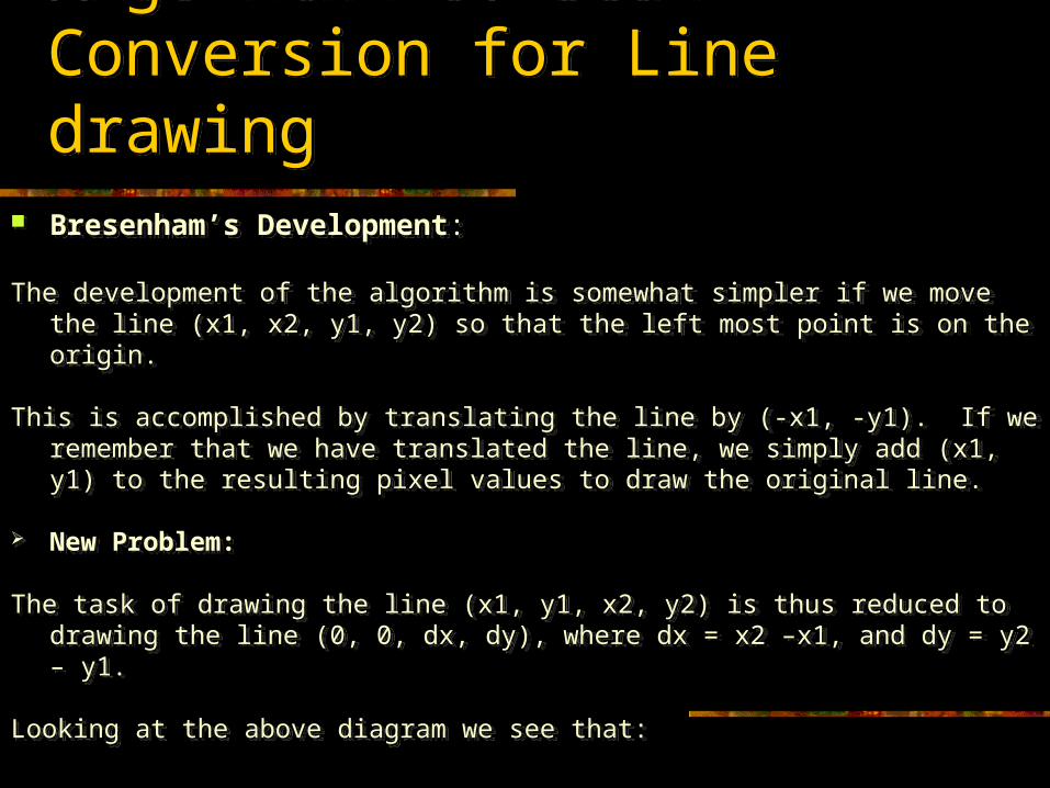
Bresenham’s Development: The development of the algorithm is somewhat simpler if we move the line (x1, x2, y1,
y2) so that the left most point is on the origin.
This is accomplished by translating the line by (-x1, -y1). If we remember that we have translated the line, we simply add (x1, y1) to the resulting pixel values to draw the original line.
New Problem:
The task of drawing the line (x1, y1, x2, y2) is thus reduced to drawing the line (0, 0, dx, dy), where dx = x2 –x1, and dy = y2 – y1.
Looking at the above diagram we see that:

Algorithm of Scan Conversion for Line drawing Algorithm of Scan Conversion for Line drawing
Bresenham’s Development: New Problem:
Looking at the above diagram we see that:
s = m * (r+1) –q, or s = dy/dx * (r+1) –qt = (q+1) - dy/dx * (r+1)
As mentioned earlier the decision whether to choose Ti or Si depends on the comparison of s and t
If s<t choose Si, else choose Ti
This decision can be reformulated as follows:
If s-t < 0 choose Si, else choose T.

Algorithm of Scan Conversion for Line drawing Algorithm of Scan Conversion for Line drawing
Bresenham’s Development: Using the definition of s and t we can compute their difference, namely
s – t = (dy/dx * (r+1) – q ) – (q+1 - dy/dx * (r+1)) = 2* dy/dx * (r+1) – 2q –1
Rearranging this equation, and multiplying by dx yields:
dx(s-t) = 2dy * (r+1) – 2q * dx - dx or = 2 * (r * dy – q * dx) + 2 * dy – dx But: notice that the quantity dx is non-zero positive. This means we can replace
the decision quantity s-t with dx(s-t)Also: notice that this quantity is an integer value

Algorithm of Scan Conversion for Line drawing Algorithm of Scan Conversion for Line drawing
Bresenham’s Development:
Decision Variable
Defining the quantity 2 * (r* dy – q * dx) + 2 * dy – dx as the decision variable D i,We can rewrite in terms of Xi-1 and Yi-1
Di = 2 * (Xi-1 * dy – Yi-1 * dx) + 2 * dy – dx
Subtracting Di from Di+1 will tell us how to compute the next decision variable
Di+1 – Di = 2* (dy ( Xi – Xi-1 ) – dx (Yi – Yi-1))
We call this error variable deltaD. We also know that Xi – Xi-1 = 1, so we have
deltaD = 2dy – 2dx (Yi – Yi-1)
Notice that this gives us two different deltaD’s depending on whether Y i – Yi-1is 1 or 0
The algorithm for drawing lines in the first octant is then described as follows:

Algorithm of Scan Conversion for Line drawing Algorithm of Scan Conversion for Line drawing
Bresenham’s Development: Bresenham’s Algorithm:
Draw_line(x1, x2, y1, y2)Integer dx = x2 –x1Integer dy = y2 – y1
d= 2dy –dxdeltaD1 = 2dydeltaD2 = 2(dy – dx)y = y1
for x from x1 to x2 by incremental step 1 set_pixel(x, y) if d < 0 then d = d + deltaD1 else d = d + deltaD2 y = y + 1 end ifend forend Draw_line

Algorithm of Scan Conversion for Line drawing Algorithm of Scan Conversion for Line drawing
Bresenham’s Development: Property of Bresenham’s Algorithm:
In the discussion above we have made some assumptions: I.e.,The slope of the line is between 0 and 1;The first point of the line is to the left of the second point; If we want to handle the cases in other octants:We can transform any line into the equivalent property as the case that first
octant has.(e.g., swap the two end points; swap the x and y values, etc….)
Property of Bresenham’s Algorithm: Simple integer arithmetic (addition operation). No floating operation, no
multiplication, no rounding function.
Extension to Mid-point algorithm (comparing the intersection point with mid-point)

Scan Converting CirclesScan Converting Circles Brute-force method
Equation of a circle centered at the origin with radius of r: x2 + y2 = r2
If the center is at (xc, yc), we may translate it to the origin, then apply scan conversion.
y = +/- sqrt(r2 – x2)
Not efficient: multiplication and square-root operation non-uniform: large gap at the place of the slope of the circle becoming infinite
Brute-force method
Equation of a circle centered at the origin with radius of r: x2 + y2 = r2
If the center is at (xc, yc), we may translate it to the origin, then apply scan conversion.
y = +/- sqrt(r2 – x2)
Not efficient: multiplication and square-root operation non-uniform: large gap at the place of the slope of the circle becoming infinite
r
yc
xc

Scan Converting CirclesScan Converting Circles Parametric Polar form:
Equation of a circle centered at the origin with radius of r: x = r cos()y = r sin()
If the center is at (xc, yc), we may translate it to the origin, then apply scan conversion.
Using a fixed angular step size, plotting the circle with equally spaced points along the circumference.
For example: The step angle delta() can be set as 1/r (= (2 ) / (2 r))
Not efficient: multiplication and trigonometric operation
Parametric Polar form:
Equation of a circle centered at the origin with radius of r: x = r cos()y = r sin()
If the center is at (xc, yc), we may translate it to the origin, then apply scan conversion.
Using a fixed angular step size, plotting the circle with equally spaced points along the circumference.
For example: The step angle delta() can be set as 1/r (= (2 ) / (2 r))
Not efficient: multiplication and trigonometric operation

Scan Converting CirclesScan Converting Circles Symmetry between octants in a circle:
Eight-way symmetry: we need to compute only one 45 degree sector (octant fromX=0 to x = y) to determine the circle completely.
Map octant I to other seven octants: I: (x,y)II: (y,x)III: (-y, x)IV: (-x, y)V: (-x, -y)VI: (-y, -x)VII: (y, -x)VIII: (x, -y)
Reducing the computation greatly
Symmetry between octants in a circle:
Eight-way symmetry: we need to compute only one 45 degree sector (octant fromX=0 to x = y) to determine the circle completely.
Map octant I to other seven octants: I: (x,y)II: (y,x)III: (-y, x)IV: (-x, y)V: (-x, -y)VI: (-y, -x)VII: (y, -x)VIII: (x, -y)
Reducing the computation greatly
I
II
VIII
VIIVI
V
IV
III
Scan Converting CirclesScan Converting Circles Mid-point circle algorithm:
Move Center (xc, yc) to (0, 0) Calculate the circle sector (octant II), where the slope of the curve varies from 0 to –1 Step in x positive direction, calculating the decision variable (or called decision
parameter) to determine the y position in each x step. Derive the position in other seven octants by symmetry Move the center (0, 0) to (xc, yc)
Mid-point circle algorithm:
Move Center (xc, yc) to (0, 0) Calculate the circle sector (octant II), where the slope of the curve varies from 0 to –1 Step in x positive direction, calculating the decision variable (or called decision
parameter) to determine the y position in each x step. Derive the position in other seven octants by symmetry Move the center (0, 0) to (xc, yc)
Scan Converting CirclesScan Converting Circles Mid-point circle algorithm:
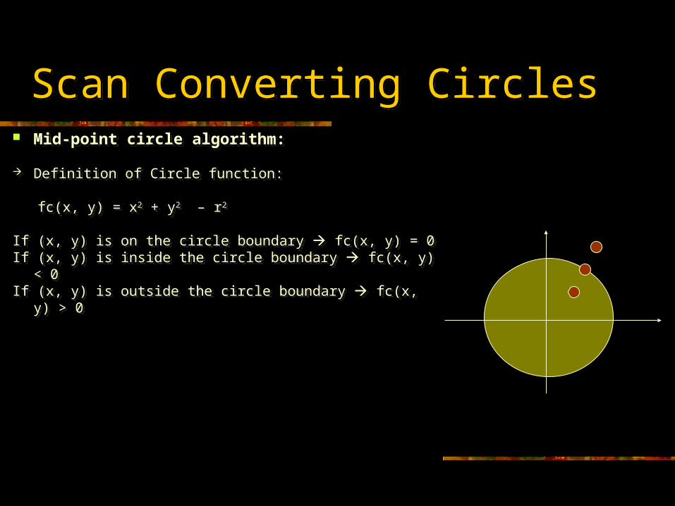
Definition of Circle function:
fc(x, y) = x2 + y2 – r2
If (x, y) is on the circle boundary fc(x, y) = 0If (x, y) is inside the circle boundary fc(x, y) < 0If (x, y) is outside the circle boundary fc(x, y) > 0
Mid-point circle algorithm:
Definition of Circle function:
fc(x, y) = x2 + y2 – r2
If (x, y) is on the circle boundary fc(x, y) = 0If (x, y) is inside the circle boundary fc(x, y) < 0If (x, y) is outside the circle boundary fc(x, y) > 0

Scan Converting CirclesScan Converting Circles Mid-point circle algorithm:
Assume the (x[k], y[k]) is determined, we need to determine the pixel position of(x[k+1], y[k+1]), which is located either at (x[k]+1, y[k]) or at (x[k]+1, y[k]-1)
Definition of Decision Variable P[k]:
The circle function in the midpoint positionP[k] = fc(x[k] + 1, y[k]- ½ ) = (x[k] + 1) 2 + (y[k] – ½ ) 2 – r2
If p[k] < 0 the midpoint is inside the circle pixel on scan line y[k] is closer to the circle boundary (x[k+1], y[k+1]) = (x[k] +1, y[k]) Else the midpoint is on or outside of the circle pixel on scan line y[k] –1 is selected (x[k+1], y[k+1]) = (x[k] +1, y[k] - 1)
Mid-point circle algorithm:
Assume the (x[k], y[k]) is determined, we need to determine the pixel position of(x[k+1], y[k+1]), which is located either at (x[k]+1, y[k]) or at (x[k]+1, y[k]-1)
Definition of Decision Variable P[k]:
The circle function in the midpoint positionP[k] = fc(x[k] + 1, y[k]- ½ ) = (x[k] + 1) 2 + (y[k] – ½ ) 2 – r2
If p[k] < 0 the midpoint is inside the circle pixel on scan line y[k] is closer to the circle boundary (x[k+1], y[k+1]) = (x[k] +1, y[k]) Else the midpoint is on or outside of the circle pixel on scan line y[k] –1 is selected (x[k+1], y[k+1]) = (x[k] +1, y[k] - 1)

Scan Converting CirclesScan Converting Circles Mid-point circle algorithm: Mid-point circle algorithm:
y[k]
y[k] -1
x[k] x[k+1]=x[k] + 1
x[k+2]=x[k] + 2
midpointx2 + y2 – r2 =0
p[k]= fc(….) p[k+1] = fc(…)

Scan Converting CirclesScan Converting Circles Mid-point circle algorithm:
Successive decision variable P[k+1]:
P[k+1] = fc(x[k+1] + 1, y[k+1]- ½ ) = (x[k] + 2)2 + (y[k+1] – ½ )2 – r2
p[k+1] = p[k] + 2(x[k]+1) + (y[k+1]2 – y[k]2 ) – (y[k+1] – y[k]) +1 If p[k] < 0 y[k+1] = y[k] Else y[k+1] = y[k] –1
Incremental calculation of decision variable:If p[k] < 0 p[k+1] – p[k] = 2x[k+1] + 1 = 2x[k] + 3Else p[k+1] – p[k] = 2x[k+1] – 2y[k+1] + 1 = 2x[k] – 2y[k] + 5
Initial starting position at (x[0], y[0]) = (0, r) decision variable p[0] = fc(1, r- ½) = 5/4 - r
Mid-point circle algorithm:
Successive decision variable P[k+1]:
P[k+1] = fc(x[k+1] + 1, y[k+1]- ½ ) = (x[k] + 2)2 + (y[k+1] – ½ )2 – r2
p[k+1] = p[k] + 2(x[k]+1) + (y[k+1]2 – y[k]2 ) – (y[k+1] – y[k]) +1 If p[k] < 0 y[k+1] = y[k] Else y[k+1] = y[k] –1
Incremental calculation of decision variable:If p[k] < 0 p[k+1] – p[k] = 2x[k+1] + 1 = 2x[k] + 3Else p[k+1] – p[k] = 2x[k+1] – 2y[k+1] + 1 = 2x[k] – 2y[k] + 5
Initial starting position at (x[0], y[0]) = (0, r) decision variable p[0] = fc(1, r- ½) = 5/4 - r

Scan Converting CirclesScan Converting Circles Mid-point circle algorithm:
/* Assume the center is at origin (0, 0) */
Input initial position of the starting point, circle center and radius Calculate initial decision variable p[0]
While(x < y) {
if p < 0 {p = p + 2x + 3;} else {p = p + 2x – 2y + 5; y = y –1;}
x = x+1;
Set circle points in the other seven octants;
}
Mid-point circle algorithm:
/* Assume the center is at origin (0, 0) */
Input initial position of the starting point, circle center and radius Calculate initial decision variable p[0]
While(x < y) {
if p < 0 {p = p + 2x + 3;} else {p = p + 2x – 2y + 5; y = y –1;}
x = x+1;
Set circle points in the other seven octants;
}

Scan Converting EllipseScan Converting Ellipse Mid-point ellipse algorithm:
Standard ellipse function at center of (0, 0):
(x/Rx) 2 + (y/Ry) 2 = 1
Ellipse function:
fe(x, y) = Ry2 * x2 + Rx2 * y2 – Rx2 * Ry2
If (x, y) is on the ellipse boundary Fe(x, y) =0If (x, y) is inside the ellipse boundary Fe(x, y) <0If (x, y) is outside the ellipse boundary Fe(x, y) >0
Mid-point ellipse algorithm:
Standard ellipse function at center of (0, 0):
(x/Rx) 2 + (y/Ry) 2 = 1
Ellipse function:
fe(x, y) = Ry2 * x2 + Rx2 * y2 – Rx2 * Ry2
If (x, y) is on the ellipse boundary Fe(x, y) =0If (x, y) is inside the ellipse boundary Fe(x, y) <0If (x, y) is outside the ellipse boundary Fe(x, y) >0

Scan Converting EllipseScan Converting Ellipse Mid-point ellipse algorithm:
Quadrant symmetry and two regions splitting within one quadrant:
Region 1: the magnitude of the slope of the curve < 1 Region 2: the magnitude of the slope of the curve >= 1
If f(x, y) = 0 dy/dx = - (df/dx) / (df/dy) = - (2* Ry2 *x ) / (2* Rx2 * y)
At the boundary between region 1 and region2: dy/dx = -1
So (2* Ry2 *x ) < (2* Rx2 * y) region1(2* Ry2 *x ) >= (2* Rx2 * y) region2
Decision Variable (or called decision parameter):
Mid-point ellipse algorithm:
Quadrant symmetry and two regions splitting within one quadrant:
Region 1: the magnitude of the slope of the curve < 1 Region 2: the magnitude of the slope of the curve >= 1
If f(x, y) = 0 dy/dx = - (df/dx) / (df/dy) = - (2* Ry2 *x ) / (2* Rx2 * y)
At the boundary between region 1 and region2: dy/dx = -1
So (2* Ry2 *x ) < (2* Rx2 * y) region1(2* Ry2 *x ) >= (2* Rx2 * y) region2
Decision Variable (or called decision parameter):
Ry
Rx
Region 1
Region 2
Slope=1
y
x

Scan Converting EllipseScan Converting Ellipse Mid-point ellipse algorithm:
Region 1: (draw region 1 until (2* Ry2 *x ) >= (2* Rx2 * y), increment in x direction)
Decision Variable (or called decision parameter):
P1[k] = fe(x[k] +1, y[k] – ½) = Ry2 (x[k]+1) 2 + Rx2 (y[k]-1/2) 2 - Rx2 Ry2
If p1[k] < 0 y[k+1] = y[k]If p1[k] >= 0 y[k+1] = y[k] –1
P1[k+1] = fe(x[k+1] +1, y[k+1] – ½)
Increment of decision variable: If p1[k] < 0 p1[k+1] – p1[k] = 2 Ry2 * x[k+1] + Ry2 If p1[k] >= 0 p1[k+1] – p1[k] = 2 Ry2 * x[k+1] + Ry2 – 2 Rx2 * y[k+1]
Initial point: (x[0], y[0]) = (0, Ry), Initial decision parameter: p1[0] = Ry2 – Rx2 * Ry + (Rx2 /4)
Mid-point ellipse algorithm:
Region 1: (draw region 1 until (2* Ry2 *x ) >= (2* Rx2 * y), increment in x direction)
Decision Variable (or called decision parameter):
P1[k] = fe(x[k] +1, y[k] – ½) = Ry2 (x[k]+1) 2 + Rx2 (y[k]-1/2) 2 - Rx2 Ry2
If p1[k] < 0 y[k+1] = y[k]If p1[k] >= 0 y[k+1] = y[k] –1
P1[k+1] = fe(x[k+1] +1, y[k+1] – ½)
Increment of decision variable: If p1[k] < 0 p1[k+1] – p1[k] = 2 Ry2 * x[k+1] + Ry2 If p1[k] >= 0 p1[k+1] – p1[k] = 2 Ry2 * x[k+1] + Ry2 – 2 Rx2 * y[k+1]
Initial point: (x[0], y[0]) = (0, Ry), Initial decision parameter: p1[0] = Ry2 – Rx2 * Ry + (Rx2 /4)

Scan Converting EllipseScan Converting Ellipse Mid-point ellipse algorithm:
Region 2: (Draw region 2 until y <=0, increment in –y direction)
Decision Variable (or called decision parameter):
P2[k] = fe(x[k] +1/2, y[k] – 1)
If p2[k] > 0 x[k+1] = x[k], y[k+1] = y[k] –1 (midpoint is outside the ellipse boundary)If p2[k] <= 0 x[k+1] = x[k] +1, y[k+1] = y[k] –1 (midpoint is inside the ellipse boundary)
P2[k+1] = fe(x[k+1] +1/2, y[k+1] – 1)
Increment of decision variable: If p2[k] > 0 p2[k+1] – p2[k] = -2 Rx2 * y[k+1] + Rx2 If p2[k] <= 0 p2[k+1] – p2[k] = 2 Ry2 * x[k+1] + Rx2 – 2 Rx2 * y[k+1]
Initial point: (x[0], y[0]) = last point calculated in region 1 Initial decision parameter: p2[0] = Ry2 * (x[0] + ½) 2 – Rx2 * (y[0] –1) 2 – Rx2 *Ry2
Mid-point ellipse algorithm:
Region 2: (Draw region 2 until y <=0, increment in –y direction)
Decision Variable (or called decision parameter):
P2[k] = fe(x[k] +1/2, y[k] – 1)
If p2[k] > 0 x[k+1] = x[k], y[k+1] = y[k] –1 (midpoint is outside the ellipse boundary)If p2[k] <= 0 x[k+1] = x[k] +1, y[k+1] = y[k] –1 (midpoint is inside the ellipse boundary)
P2[k+1] = fe(x[k+1] +1/2, y[k+1] – 1)
Increment of decision variable: If p2[k] > 0 p2[k+1] – p2[k] = -2 Rx2 * y[k+1] + Rx2 If p2[k] <= 0 p2[k+1] – p2[k] = 2 Ry2 * x[k+1] + Rx2 – 2 Rx2 * y[k+1]
Initial point: (x[0], y[0]) = last point calculated in region 1 Initial decision parameter: p2[0] = Ry2 * (x[0] + ½) 2 – Rx2 * (y[0] –1) 2 – Rx2 *Ry2

Scan Converting Other CurvesScan Converting Other Curves Other curves:
Conics (circle, ellipse, parabolas, hyperbolas: Ax2 + By2 + Cxy + Dx + Ey + F=0) trigonometric (e.g., periodical symmetry or repeating) exponential functions probability distributions (e.g., symmetry along the mean) general polynomial and spline curves y = a[0] + a[1] x + ….+ a[n-1] xn-1 + a[n] x n
Quadratic: n=2Cubic polynomial: n = 3Quartic: n =4Straight line: n = 1
E.g., Spline curves: formed by cubic polynomial pieces on a set of discrete points,Which is constrained by a certain smooth and continuous conditions
Applications:
E.g., object surface modeling; Animation path design data and function graphing and visualization
Other curves:
Conics (circle, ellipse, parabolas, hyperbolas: Ax2 + By2 + Cxy + Dx + Ey + F=0) trigonometric (e.g., periodical symmetry or repeating) exponential functions probability distributions (e.g., symmetry along the mean) general polynomial and spline curves y = a[0] + a[1] x + ….+ a[n-1] xn-1 + a[n] x n
Quadratic: n=2Cubic polynomial: n = 3Quartic: n =4Straight line: n = 1
E.g., Spline curves: formed by cubic polynomial pieces on a set of discrete points,Which is constrained by a certain smooth and continuous conditions
Applications:
E.g., object surface modeling; Animation path design data and function graphing and visualization
Scan Converting Other CurvesScan Converting Other Curves Function representation:
explicit y = f(x) parametric representation: x = f(); y = f() implicit f(x, y) = 0
Drawing methods: explicit: direct drawing (brute-force) or Incremental method (DDA, mid-point, Bresenham) parametric: direct drawing (brute-force) or incremental method (DDA, mid-point, Bresenham) implicit: f(x, y) = 0: Incremental method similar to the mid-point method
For function of y = f(x):If the slope had magnitude <= 1, drawing in the x incremental directionIf the slope had magnitude > 1, drawing in the y incremental direction
Taking advantage of the symmetry property, if any Curve functions: example in OpenGL (curve and surface evaluator)
Discrete data set: Approximation/curve-fitting and interpolation(passing through control points) Piece-wise line segment representation for curves and discrete data set
Function representation:
explicit y = f(x) parametric representation: x = f(); y = f() implicit f(x, y) = 0
Drawing methods: explicit: direct drawing (brute-force) or Incremental method (DDA, mid-point, Bresenham) parametric: direct drawing (brute-force) or incremental method (DDA, mid-point, Bresenham) implicit: f(x, y) = 0: Incremental method similar to the mid-point method
For function of y = f(x):If the slope had magnitude <= 1, drawing in the x incremental directionIf the slope had magnitude > 1, drawing in the y incremental direction
Taking advantage of the symmetry property, if any Curve functions: example in OpenGL (curve and surface evaluator)
Discrete data set: Approximation/curve-fitting and interpolation(passing through control points) Piece-wise line segment representation for curves and discrete data set
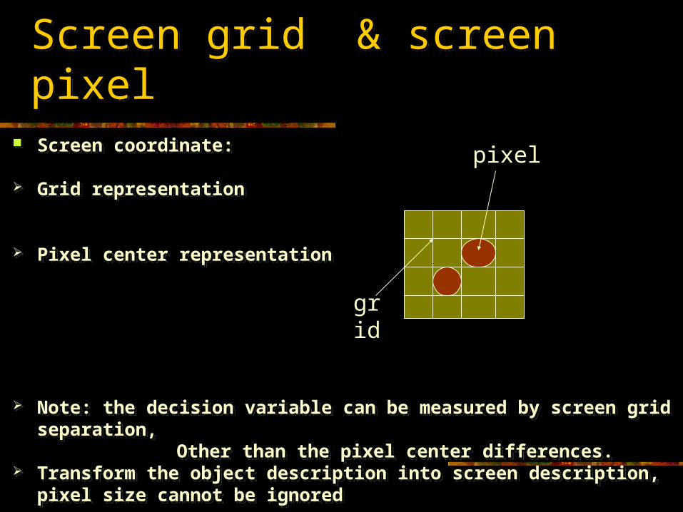
Screen grid & screen pixelScreen grid & screen pixel Screen coordinate:
Grid representation
Pixel center representation
Note: the decision variable can be measured by screen grid separation, Other than the pixel center differences. Transform the object description into screen description, pixel size
cannot be ignored
Screen coordinate:
Grid representation
Pixel center representation
Note: the decision variable can be measured by screen grid separation, Other than the pixel center differences. Transform the object description into screen description, pixel size
cannot be ignored
grid
pixel

Issues to be consideredIssues to be considered Aliasing
Jagged or stairstep appearance due to the raster algorithm
The sampling process digitizes coordinate points on an object to discrete integer pixel positions.
Low-frequency sampling (undersampling)
Antialiasing
Reducing the aliasing effect, improving the undersampling process.
Aliasing
Jagged or stairstep appearance due to the raster algorithm
The sampling process digitizes coordinate points on an object to discrete integer pixel positions.
Low-frequency sampling (undersampling)
Antialiasing
Reducing the aliasing effect, improving the undersampling process.
![PYTHON OBJECT MODEL · Object Oriented Programming 13 r = Rectangle(x1,y1,x2,y2) [constructor] Create a new rectangle rfrom four integers: x1, y1, x2, y2 Our domain is the two-dimensional](https://img.pdfslide.us/doc/110x75/5f61df18d5c516736030a6b4/python-object-model-object-oriented-programming-13-r-rectanglex1y1x2y2-constructor.jpg)


![Section 1 1 Outline.doc · Web viewDistance formula: ([x2 – x1]2 + [y2 – y1]2 . Midpoint of segment with endpoints (x1, y1) and (x2, y2) is ([x1+x2]/2, [y1+y2]/2) Five Minute](https://img.pdfslide.us/doc/110x75/6097fb3540141924900c4198/section-1-1-outlinedoc-web-view-distance-formula-x2-a-x12-y2-a-y12.jpg)
![Audio Content Analysis - Laboratory Course · 2013. 5. 15. · 4 5 function[y1,y2] =my_function(x1,x2) 6 7 y1=x2; 8 y2=x1; EinführungTermin 1Termin 2Termin 3Termin 4 ... 16 thisValue=my_function(thisFrame);](https://img.pdfslide.us/doc/110x75/6097fb3240141924900c4187/audio-content-analysis-laboratory-2013-5-15-4-5-functiony1y2-myfunctionx1x2.jpg)

![IT DESCRIZIONE - PULIZIA - CARATTERISTICHE TECNICHE EN ... · 2 [cm] x1 80 x2 10 y1 10 y2 10 z 60 y2 x1 x2 z y1 rimozione dalla paletta - scoop removal - pellet deplacement schaufel](https://img.pdfslide.us/doc/110x75/5e48b074eda53c60a3544345/it-descrizione-pulizia-caratteristiche-tecniche-en-2-cm-x1-80-x2-10-y1.jpg)