Embed Size (px)
Citation preview
HAL Id: hal-01244663https://hal.inria.fr/hal-01244663
Submitted on 16 Dec 2015
HAL is a multi-disciplinary open accessarchive for the deposit and dissemination of sci-entific research documents, whether they are pub-lished or not. The documents may come fromteaching and research institutions in France orabroad, or from public or private research centers.
L’archive ouverte pluridisciplinaire HAL, estdestinée au dépôt et à la diffusion de documentsscientifiques de niveau recherche, publiés ou non,émanant des établissements d’enseignement et derecherche français ou étrangers, des laboratoirespublics ou privés.
Scaling Out Link Prediction with SNAPLEAnne-Marie Kermarrec, François Taïani, Juan Manuel Tirado Martin
To cite this version:Anne-Marie Kermarrec, François Taïani, Juan Manuel Tirado Martin. Scaling Out Link Predic-tion with SNAPLE. 16th Annual ACM/IFIP/USENIX Middleware Conference, Dec 2015, Vancouver,Canada. pp.12, �10.1145/2814576.2814810�. �hal-01244663�
Scaling Out Link Prediction with SNAPLE:1 Billion Edges and Beyond
Anne-Marie KermarrecINRIA Rennes, France
Francois TaianiU. of Rennes 1 - IRISA - ESIR
Rennes, [email protected]
Juan M. Tirado∗
University of CambridgeCambridge UK
ABSTRACTA growing number of organizations are seeking to analyzeextra large graphs in a timely and resource-efficient manner.With some graphs containing well over a billion elements,these organizations are turning to distributed graph-computing platforms that can scale out easily in existingdata-centers and clouds. Unfortunately such platformsusually impose programming models that can be ill suitedto typical graph computations, fundamentally underminingtheir potential benefits.
In this paper, we consider how the emblematic problemof link-prediction can be implemented efficiently in gather-apply-scatter (GAS) platforms, a popular distributed graph-computation model. Our proposal, called Snaple, exploitsa novel highly-localized vertex scoring technique, andminimizes the cost of data flow while maintaining predictionquality. When used within GraphLab, Snaple can scale tovery large graphs that a standard implementation of linkprediction on GraphLab cannot handle. More precisely, weshow that Snaple can process a graph containing 1.4 billionsedges on a 256 cores cluster in less than three minutes,with no penalty in the quality of predictions. This resultcorresponds to an over-linear speedup of 30 against a 20-corestandalone machine running a non-distributed state-of-the-art solution.
Keywordslink prediction, graph processing, parallelism, distribution,scalability
1. INTRODUCTIONGraph computing is today emerging as a critical service
for many large-scale on-line applications. Companies suchas Twitter, Facebook, and Linked-In are capturing, storing,and analyzing increasingly large amounts of connected data
∗The work presented was performed while Juan was withInria.
stored as graphs. As the size of these graphs increases, thesecompanies are moving away from standalone one-machinedeployments [12] and are instead looking for distributedsolutions [27, 25] that can harvest the resources of multiplemachines to process these graphs in parallel. Distributionunfortunately comes with an extra complexity, which canconsiderably hamper a solution’s scalability if not properlymanaged. To work around this challenge, distributed graphprocessing engines1 offer optimized programming models(gather-apply-scatter, bulk synchronous processing [43])that limit the propagation of data to well-defined pointsof the execution and the graph. Fitting an existing graphalgorithm to these models, while controlling the networkingcosts this creates, is unfortunately a difficult task thatremains today more a craft than a science.
In this paper, we focus on the particular problem oflink-prediction [22] in large graphs, an emblematic graphanalysis task that appears in numerous applications (contentrecommendations, advertising, social mining, forensics).Implementing link prediction on a distributed graph engineraises two critical challenges: (1) traditional link predictionapproaches are ill-fitted to the programming models ofgraph processing engines; (2) because of this bad fitcommunication costs can be difficult to keep under control,reducing the benefits of distribution.
More precisely, the link prediction problem considers agraphG in which some edges are missing, and tries to predictthese missing edges. To be able to scale, most practicalsolutions search for missing edges in the vicinity of individualvertices, using bounded graph traversal techniques such asbounded random walks, or d-hops neighborhood traversal.
Unfortunately, these graph traversal techniques requireslarge amounts of information to be propagated betweenvertices, and do not lend themselves to the highly localizedmodels offered by distributed graph engines, such as theBulk Synchronous Processing (BSP) model of Pregel [27], orthe Gather Apply Scatter (GAS) model of GraphLab [25].In both cases, a naive application of traversal techniquesrequires vertex information to be replicated to maintainlocality, and can lead to high communication and memorycosts. This is particularly true of graphs in which thelikelihood of two vertices being neighbors can be computedeasily, but which require large amounts of information to beshared between vertices, such as in social graphs with largeuser profiles.
In this paper, we propose a highly scalable approach tolink-prediction that can be implemented efficiently within
1distributed graph engines for short

the Gather Apply Scatter (GAS) model. The resultingsystem, called Snaple, relies on a scoring framework ofpotential edges that eschews large data flows along graphedges. Instead, Snaple combines and aggregates similarityscores along the paths of the original graph, and thusavoids explicit and costly graph traversal operations. Wedemonstrate the benefits of Snaple with a prototype basedon Graphlab [25], which we evaluate using real datasetsdeployed on top of a testbed with 32 nodes and 256cores. Our experiments show that Snaple’s performancegoes well beyond that of a standard GAS implementation,and is able to process a graph containing 1.4 billionsedges in 2min57s on our testbed, when a naive GraphLabversion fails due to resource exhaustion. We obtain theseresults with no penalty in prediction quality comparedto a traditional approach. Snaple further demonstrateslinear or over-linear speedups in computation time againsta single machine deployment running a state-of-the-art non-distributed solution while improving predictions.
In the following we first describe link-prediction in moredetail, and introduce the Gather Scatter Apply (GAS)programming model (Section 2). In Section 3, we presentthe principles of Snaple, our link prediction framework. Wethen detail how Snaple can be implemented efficiently on aGAS engine in Section 4. Section 5 presents an exhaustiveevaluation of our approach. Finally, Section 6 discussesrelated work, and Section 7 concludes.
2. BACKGROUND AND PROBLEM
2.1 Link-prediction.Link prediction [22] seeks to predict missing edges from
a graph G. Edges might be missing because the graph isevolving over time (users create new social links), or becauseG only captures a part of a wider ground truth. Predictededges can be used to recommend new users (social graphs),new items (bipartite graph), or uncover missing information(social mining).
Formally, link prediction considers two graphs2 G =(V,E) and G′ = (V,E′) so that G contains less informationthan G′ in the form of missing edges: E ( E′. For instanceG and G′ might represent the same social graph captured atdifferent points in time, or G might represent an incompletesnapshot of a larger graph represented by G′ (an interactionnetwork, a set of related topics, etc.). The goal of linkprediction is then to predict which are the edges of G′ thatG lacks, i.e. to determine E′ \ E.
Link prediction strategies fall into unsupervised and su-pervised approaches. The typical approach for unsupervisedlink prediction is sketched in Algorithm 1. The algorithmexecutes a parallelizable loop that iterates through allvertices of G (lines 1-3). Each iteration hinges on the scoringfunction score(u, z) (line 2) which reflects how likely the edge(u, z) is to appear in G′. In this basic version, the algorithmscores all vertices z that are not already in u’s neighborhood(noted ΓG(u) = {v ∈ V |(u, v) ∈ E}), and returns the kvertices with the highest scores as predicted neighbors for u(operator argtopk).
The function score(u, z) may only use topological proper-
2For brevity’s sake, we consider directed graphs in our ex-planations, but the same principles carry over to undirectedgraphs.
Algorithm 1 Unsupervised top k link-prediction
Require: k,score1: for u ∈ V do2: predictionu ← argtopk
z∈V \ΓG(u)
(score(u, z)
)3: end for
ties, such as the connectivity-based metrics proposed in theseminal work of Liben-Nowell and Kleinberg [22] (e.g. thenumber of common neighbors between u and z, |ΓG(u) ∩ΓG(z)|). This score may also exploit vertex content, i.e.the additional application-dependent knowledge attached tovertices [7, 16, 31, 32, 39], such as user profiles, tags, ordocuments. In many domains, pure topological metricstend to be the main drivers of link generation, and aretherefore almost always present in the prediction process.Scoring functions using only topological metrics are alsomore generic as they do not rely on information that isexternal to the graph (tags, content, user profiles, etc.) andmight not be available in all data sets.
Supervised approaches build upon unsupervised strategiesand leverage machine-learning algorithms to produce opti-mized scoring functions [23, 38]. Supervised approaches tendto perform better, but at the cost of an important learningeffort, as they must often scan the whole graph to build anaccurate classification model. In this paper, we thereforefocus on unsupervised approaches, but the key ideas wepresent can be extended to supervised schemes.
2.2 Scaling link predictionWhile research on link prediction originally sought to
maximize the quality of predicted edges, with little consider-ation for computation costs, its practical relevance for socialnetworks and recommendation services has put it at theforefront of current system research. One critical challengefaced by current implementations is the fast growing size ofthe graphs they must process [12, 21].
A first strategy to scale Algorithm 1 is to improvethe performance of individual iterations. A frequentoptimization limits the search for missing edges to thevicinity of individual vertices. If one notes ΓKG (u) the K-hop neighborhood of u in G, defined recursively as
Γ1G(u) = ΓG(u)
ΓKG (u) = ΓK−1G (u) ∪ {z ∈ V |∃v ∈ ΓK−1
G (u) : (v, z) ∈ E}(1)
this optimization will only consider the vertices of ΓKG (u) \ΓG(u) at line 2 as potential new neighbors in G′ (Equation 2below), instead of the much larger set V \ ΓG(u). K isgenerally small (2 or 3). We use K = 2 in this work.
predictionu ← argtopk
z∈ΓKG
(u)\ΓG(u)
(score(u, z)
)(2)
This optimization works well because social graphs, andfield graphs in general, tend to present high clusteringcoefficients. As a result, most of the edges to be predictedin G′ will connect vertices only separated by a few hopsin G [44]. Other optimizations on standalone machinesleverage specialized data structures and memory layout toexploits data locality and minimize computing costs [20, 33].
A second strategy seeks to scale Algorithm 1 horizontallyby deploying it onto a distributed infrastructure. That isthe case of Twitter for instance, who recently moved their
Who-to-Follow service to a distributed solution, from aninitial single machine deployment [12]. This transition canleverage a growing number of graph processing engines [5, 6,12, 15, 17, 26, 27, 34], which aim to facilitate the realizationof scalable graph processing tasks. These engines do soby implementing highly parallelizable programming modelssuch as Bulk Synchronous Processing (BSP) [17, 27, 34, 43],or Gather, Apply, Scatter (GAS) [25] .
2.3 The GAS modelIn this work, we focus particularly on the GAS model,
which can be seen as a refinement of map-reduce and BSPfor graphs. Its reference implementation, GraphLab [11, 25],is particularly scalable, and was found to perform best in arecent comparison of modern graph engines across a numberof typical graph computing tasks [13].
More precisely, a GAS program assumes every vertexu ∈ V and every edge (u, v) ∈ E of a graph G = (V,E)is associated with some mutable data, noted Du and D(u,v).A GAS program consists of a sequence of GAS super-steps(or steps). Each step comprises three conceptual phases thatexecute in parallel at each vertex and manipulate these data.(Our notation follows closely that of [11].)
1. The gather phase is similar to a map-and-reduce step.This phase collects the data associated with a vertexu’s neighbors ΓG(u) and with u’s out-going3 edges{u}×ΓG(u). It maps this data through a user-providedgather() function; and aggregates the result using ageneral sum() function defined by the user.
Σ← sumv∈ΓG(u)
{gather(Du, D(u,v), Dv)
}(3)
2. In the apply phase, the result of the gather phase, Σ, isused to update the current data of node u, Du, usinga user-defined apply function.
D′u ← apply(Σ, Du
)(4)
3. Finally the scatter phase uses Σ and the new value ofDu to propagate information within u’s neighborhoodusing a scatter function provided by the user.
∀v ∈ Γ−1G (u) : D′(v,u) ← scatter
(Σ, D′u, D(v,u)
)(5)
2.4 Link prediction in the GAS modelThe GAS model facilitates the scheduling and paral-
lelization of vertex operations while increasing contentlocality. GAS engines, however, can require some substantialeffort to adapt existing graph algorithms, for two reasons.First, graph traversals, a primitive strategy of many graphalgorithms, are difficult to express in the GAS paradigmwithout adding substantial complexity and overhead. Thisis because the accesses and updates of a GAS step are limitedto adjacent vertices and edges.
The second difficulty pertains to the limited access totopological information offered by the GAS paradigm. Inthe GAS model, vertices drive and organize the computation(principally in the gather and scatter phases), but arenot expected to be an object of computation per se, in
3We present here the case in which the gather phase workson out-going edges and the scatter phase on incoming edges,but the GAS model can also use edges in the reversedirection, or even treat all edges symmetrically.
...
...
...
c
bd
e f
a a
...
...
...
N0 N1 N2
c : ΓG(c)d : ΓG(d)e : ΓG(e)
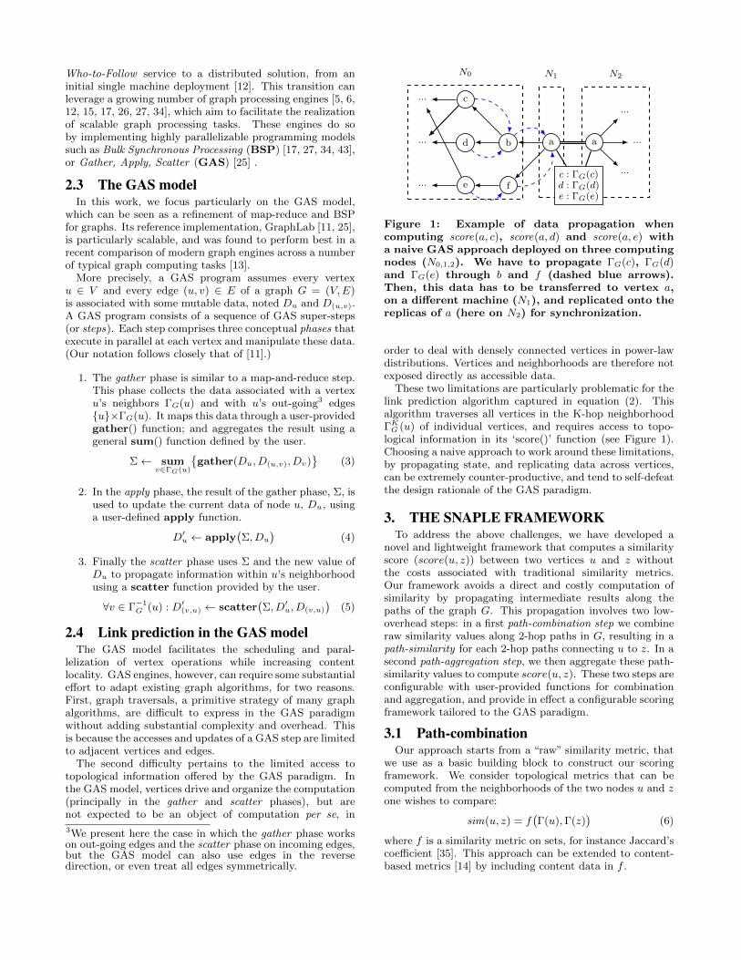
Figure 1: Example of data propagation whencomputing score(a, c), score(a, d) and score(a, e) witha naive GAS approach deployed on three computingnodes (N0,1,2). We have to propagate ΓG(c), ΓG(d)and ΓG(e) through b and f (dashed blue arrows).Then, this data has to be transferred to vertex a,on a different machine (N1), and replicated onto thereplicas of a (here on N2) for synchronization.
order to deal with densely connected vertices in power-lawdistributions. Vertices and neighborhoods are therefore notexposed directly as accessible data.
These two limitations are particularly problematic for thelink prediction algorithm captured in equation (2). Thisalgorithm traverses all vertices in the K-hop neighborhoodΓKG (u) of individual vertices, and requires access to topo-logical information in its ‘score()’ function (see Figure 1).Choosing a naive approach to work around these limitations,by propagating state, and replicating data across vertices,can be extremely counter-productive, and tend to self-defeatthe design rationale of the GAS paradigm.
3. THE SNAPLE FRAMEWORKTo address the above challenges, we have developed a
novel and lightweight framework that computes a similarityscore (score(u, z)) between two vertices u and z withoutthe costs associated with traditional similarity metrics.Our framework avoids a direct and costly computation ofsimilarity by propagating intermediate results along thepaths of the graph G. This propagation involves two low-overhead steps: in a first path-combination step we combineraw similarity values along 2-hop paths in G, resulting in apath-similarity for each 2-hop paths connecting u to z. In asecond path-aggregation step, we then aggregate these path-similarity values to compute score(u, z). These two steps areconfigurable with user-provided functions for combinationand aggregation, and provide in effect a configurable scoringframework tailored to the GAS paradigm.
3.1 Path-combinationOur approach starts from a “raw” similarity metric, that
we use as a basic building block to construct our scoringframework. We consider topological metrics that can becomputed from the neighborhoods of the two nodes u and zone wishes to compare:
sim(u, z) = f(Γ(u),Γ(z)
)(6)
where f is a similarity metric on sets, for instance Jaccard’scoefficient [35]. This approach can be extended to content-based metrics [14] by including content data in f .
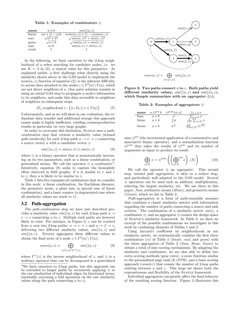
Table 1: Examples of combinators ⊗
name a⊗ b sim?v(u, z)
linear αa+ (1− α)b αsim(u, v) + (1− α)sim(v, z)
eucl√a2 + b2
√sim(u, v)2 + sim(v, z)2
geom√a× b
√sim(u, v)× sim(v, z)
sum a+b sim(u, v) + sim(v, z)count 1 1
In the following, we limit ourselves to the 2-hop neigh-borhood of u when searching for candidate nodes, i.e. weuse K = 2 in (2), a typical value for this parameter. Asexplained earlier, a first challenge when directly using thesimilarity shown above in the GAS model to implement thescore(u, z) function of equation (2), is the inherent difficultyto access data attached to the nodes z ∈ Γ2(u)\Γ(u), whichare not direct neighbors of u. One naive solution consists inusing an initial GAS step to propagate a node’s informationto its neighbors, and make this data accessible to neighborsof neighbors in subsequent steps.
D′u.neighborhood ←{
(v,Dv)∣∣ v ∈ Γ(u)
}(7)
Unfortunately, and as we will show in our evaluation, the re-dundant data transfer and additional storage this approachcauses make it highly inefficient, yielding counterproductiveresults in particular on very large graphs.
In order to overcome this limitation, Snaple uses a path-combination step that returns a similarity value (termedpath-similarity) for each 2-hop path u → v → z connectinga source vertex u with a candidate vertex z:
sim?v(u, z) = sim(u, v)⊗ sim(v, z) (8)
where ⊗ is a binary operator that is monotonically increas-ing on its two parameters, such as a linear combination, orgeneralized means. We call the operator ⊗ a combinator4.Intuitively, equation (8) seeks to capture the homophilyoften observed in field graphs: if u is similar to v and vto z, then u is likely to be similar to z.
Table 1 lists five examples of combinators that we considerin this work: a linear combination, the Euclidean distance,the geometric mean, a plain sum (a special case of linearcombination), and a basic counter (a degenerated case whereall similarity values are stuck to 1).
3.2 Path-aggregationThe path-combination step we have just described pro-
vides a similarity value sim?v(u, z) for each 2-hop path u→
v → z connecting u to z. Multiple such paths are howeverlikely to exist. For instance, in Figure 2, z can be reachedfrom u over two 2-hop paths: u → v → z and u → f → z,delivering two different similarity values, sim?
v(u, z) andsim?
f (u, z). Snaple aggregates these different values to
obtain the final score of a node z ∈ Γ2(u) \ Γ(u):
score(u, z) =⊕
v∈Γ(u)∩Γ-1(z)
sim?v(u, z) (9)
where Γ-1(z) is the inverse neighborhood of z, and ⊕ is amultiary operator that can be decomposed in a generalized4We limit ourselves to 2-hop paths, but this approach canbe extended to longer paths by recursively applying ⊗ tothe raw similarities of individual edges (in functional terms,essentially executing a fold operation on the raw similarityvalues along the path connecting u to z).
u v
x
y
zf
sim(u, v)
sim(v, x)
sim(v, y)
sim(v, z)
sim(u, f)
sim(f, z)
score(u, z) =⊕
w∈{v,f}sim?
w(u, z)
Figure 2: Two paths connect u to z. Both paths yielddifferent similarity values, sim?
v(u, z) and sim?f (u, z),
which Snaple summarizes with an aggregator (⊕).
Table 2: Examples of aggregators ⊕
name a⊕pre b ⊕post(σ, n) ⊕x∈XxSum a+ b σ
∑x∈X x
Mean a+ b 1nσ 1
|X|∑x∈X x
Geom a× b σ1n (
∏x∈X x)
1|X|
sum ⊕pre (the incremental application of a commutative andassociative binary operator), and a normalization function⊕post that takes the results of ⊕pre and its number ofarguments as input to produce its result:⊕
x∈X
x = ⊕post
((⊕x∈X
prex
), |X|
)(10)
We call the operator ⊕ an aggregator. This secondstep, termed path aggregation, is akin to a reduce step,and particularly well adapted to the GAS model. Several⊕ operators can be used such as addition, multiplication,selecting the largest similarity, etc. We use three in thispaper, Sum, arithmetic means (Mean), and geometric means(Geom), which we list in Table 2.
Path-aggregation is a form of path-ensemble measurethat combines a classic similarity metrics with informationregarding the number of paths connecting a source and sinkvertices. The combination of a similarity metric sim(), acombinator ⊗, and an aggregator ⊕ creates the design spaceof Snaple’s similarity framework. In Table 3, we show anexcerpt of the possible combinations we investigate in thiswork by combining elements of Tables 1 and 2.
Using Jaccard’s coefficient on neighborhoods as oursimilarity metric, we systematically combine the first threecombinators (⊕) of Table 1 (linear, eucl, and geom) withthe three aggregators of Table 2 (Sum, Mean, Geom) toobtain a total of nine scoring mechanisms. By adapting thesimilarity and combinator, we are also able to define twoextra scoring methods (gray rows): a score function similarto the personalized page rank [4] (PPR), and a basic scoringapproach (counter) that counts the number of 2-hop pathsexisting between u and z. This large set shows both theexpressiveness and flexibility of the Snaple framework.
Individual aggregators can greatly affect the final behaviorof the resulting scoring function. Figure 3 illustrates this
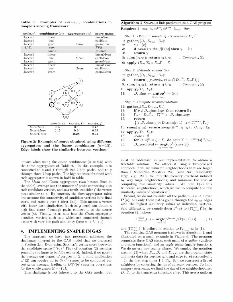
Table 3: Examples of score(u, z) combinations inSnaple’s scoring framework
sim(u, v) combinator (⊗) aggregator (⊕) score nameJaccard linear
Sum
linearSumJaccard eucl euclSumJaccard geom geomSum1/|Γv | sum PPR
– count counterJaccard linear
MeanlinearMean
Jaccard eucl euclMeanJaccard geom geomMeanJaccard linear
GeomlinearGeom
Jaccard eucl euclGeomJaccard geom geomGeom
a
b
c
d
e
f
g
h
0.5
0.1
0.2
0.1
0.3
0.20.3
0.2
0.2
0
0
score(a, e) score(a, f) score(a, g)linearSum 0.3 0.6 0.75linearMean 0.15 0.3 0.25linearGeom 0 0.28 0.24
Figure 3: Example of scores obtained using differentaggregators and the linear combinator (α=0.5).Edge labels show the similarity between vertices.
impact when using the linear combinator (α = 0.5) withthe three aggregators of Table 2. In this example, a isconnected to e and f through two 2-hop paths, and to gthrough three 2-hop paths. The highest score obtained witheach aggregator is shown in bold in table.
The Mean and Geom aggregators (two bottom lines inthe table), average out the number of paths connecting a toeach candidate vertices, and as a result, consider f the vertexmost similar to a. By contrast, the Sum aggregator takesinto account the connectivity of candidate vertices in its finalscore, and rates g over f (first line). This means a vertexwith lower path-similarities (such as g here) can obtain ahigh final score if enough paths connect it to the sourcevertex (a). Finally, let us note how the Geom aggregatorpenalizes vertices such as e which are connected throughpaths with very low path-similarity (here a → h → e).
4. IMPLEMENTING SNAPLE IN GASThe approach we have just presented addresses the
challenges inherent to the GAS model that we discussedin Section 2.4. Even using Snaple’s vertex score however,the candidate space Γ2(u) \ Γ(u) of equation (2) remainsgenerally too large to be fully explored. Indeed, if we note nthe average out-degree of vertices in G, a blind applicationof (2) can require up to O(n2) scores to be computed pervertex on average, leading to O(|V |n2) scoring operationsfor the whole graph G = (V,E).
This challenge is not inherent to the GAS model, but
Algorithm 2 Snaple’s link-prediction as a GAS program
Require: k, sim, ⊗, ⊕pre, ⊕post, klocal, thrΓ
. Step 1: Obtain a sample of u’s neighbors Du.Γ
1: gather1(Du, D(u,v), Dv):2: γ ← {v}3: if rand() > thrΓ/|Γ(u)| then γ ← ∅ ;4: return γ
5: sum1(γ1,γ2): return γ1 ∪ γ2 . Computing Σ1
6: apply1(Du, Σ1): Du.Γ← Σ1
. Step 2: Estimate similarities
7: gather2(Du, D(u,v), Dv):
8: return{(v, sim(u, v) ≡ f(Du.Γ , Dv.Γ )
)}9: sum2(γ1,γ2): return γ1 ∪ γ2 . Computing Σ2
10: apply2(Du, Σ2):
11: Du.sims← argtopklocal
(v,sv)∈Σ2
(sv)
. Step 3: Compute recommendations
12: gather3(Du, D(u,v), Dv):13: if v 6∈ Du.sims.keys then return ∅ ;14: Γu ← Du.Γu ; Γmaxv ← Dv.sims.keys15: return{
(z,Du.sims[v]⊗Dv.sims[z], 1)∣∣ z ∈ Γmaxv \ Γu
}16: sum3(γ1,γ2): return merge(⊕pre, γ1, γ2) . Comp. Σ3
17: apply3(Du, Σ3):18: score ← ∅19: for (z, spre
z , nz) ∈ Σ3 do score[z]← ⊕post(sprez , nz)
20: Du.predicted← argtopk
z∈score.keys
(score[z]
)
must be addressed in our implementation to obtain atractable solution. We attack it using a two-prongedapproach: first, we truncate neighborhoods that are largerthan a truncation threshold thrΓ (with thrΓ reasonablylarge, e.g. 200), to limit the memory overhead inducedby very large neighborhoods, and minimize the cost ofcomputing raw similarity values. We note Γ(u) thistruncated neighborhood, which we use to compute the rawsimilarity values of equation (6).
Second, we do not consider all the paths u→ v → z overΓ2(u), but only those paths going through the klocal edgeswith the highest similarity values at individual vertices.
Said differently, we sample down Γ2(u) to(Γmaxklocal
)2(u) in
equation (2), where
Γmaxklocal(u) = argtopklocal
v∈Γ(u)
f(Γ(u), Γ(z)
)(11)
and (Γmaxklocal)2 is defined in relation to Γklocal as in (1).
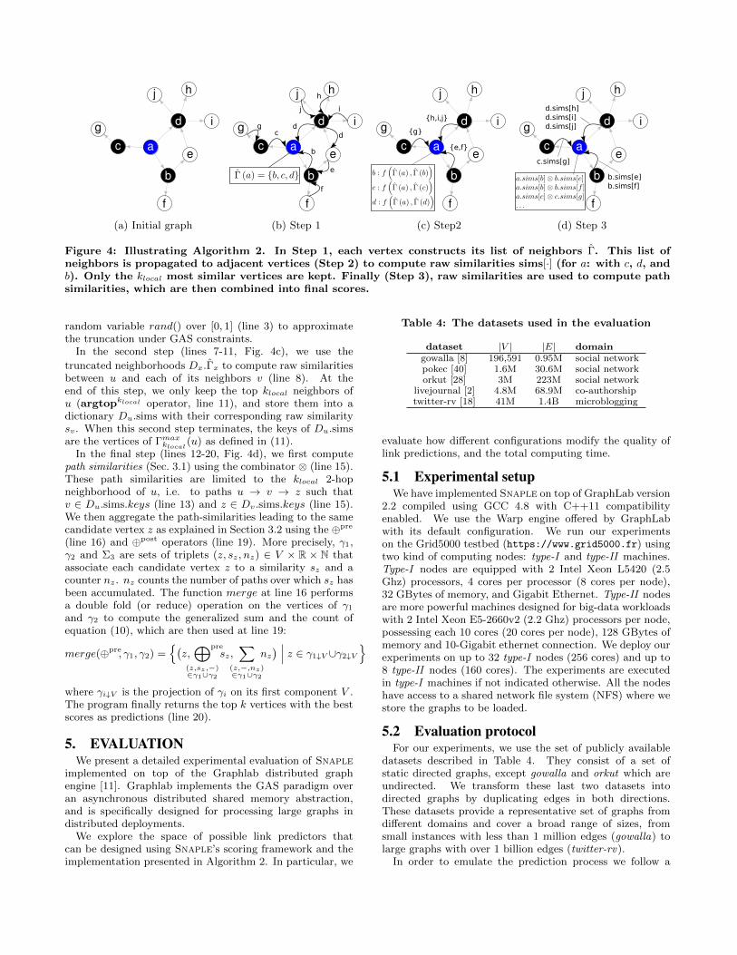
The resulting GAS program is shown in Algorithm 2, andillustrated on a small example in Figure 4. The programcomprises three GAS steps, each made of a gather (gatherand sum functions), and an apply phase (apply function).We do no use any scatter phase. We employ the notationused in [25] where Du, Dv and D(u,v) are the program stateand meta-data for vertices u, v and edge (u, v) respectively.
In the first step (lines 1-6, Fig. 4b), we construct a list ofneighbors by collecting the ids of adjacent vertices. To limitmemory overheads, we limit the size of the neighborhood setDu.Γu to the truncation threshold thrΓ. This uses a uniform
(a) Initial graph
cd
b
f
e
d
i
h
j
g
(b) Step 1
{g}
{h,i,j}
{e,f}
(c) Step2
c.sims[g]
d.sims[h]d.sims[i]d.sims[j]
b.sims[e]b.sims[f]
(d) Step 3
Figure 4: Illustrating Algorithm 2. In Step 1, each vertex constructs its list of neighbors Γ. This list ofneighbors is propagated to adjacent vertices (Step 2) to compute raw similarities sims[·] (for a: with c, d, andb). Only the klocal most similar vertices are kept. Finally (Step 3), raw similarities are used to compute pathsimilarities, which are then combined into final scores.
random variable rand() over [0, 1] (line 3) to approximatethe truncation under GAS constraints.
In the second step (lines 7-11, Fig. 4c), we use the
truncated neighborhoods Dx.Γx to compute raw similaritiesbetween u and each of its neighbors v (line 8). At theend of this step, we only keep the top klocal neighbors ofu (argtopklocal operator, line 11), and store them into adictionary Du.sims with their corresponding raw similaritysv. When this second step terminates, the keys of Du.simsare the vertices of Γmaxklocal
(u) as defined in (11).In the final step (lines 12-20, Fig. 4d), we first compute
path similarities (Sec. 3.1) using the combinator ⊗ (line 15).These path similarities are limited to the klocal 2-hopneighborhood of u, i.e. to paths u → v → z such thatv ∈ Du.sims.keys (line 13) and z ∈ Dv.sims.keys (line 15).We then aggregate the path-similarities leading to the samecandidate vertex z as explained in Section 3.2 using the ⊕pre
(line 16) and ⊕post operators (line 19). More precisely, γ1,γ2 and Σ3 are sets of triplets (z, sz, nz) ∈ V × R × N thatassociate each candidate vertex z to a similarity sz and acounter nz. nz counts the number of paths over which sz hasbeen accumulated. The function merge at line 16 performsa double fold (or reduce) operation on the vertices of γ1
and γ2 to compute the generalized sum and the count ofequation (10), which are then used at line 19:
merge(⊕pre, γ1, γ2) ={(z,⊕pre
(z,sz ,−)∈γ1∪γ2
sz,∑
(z,−,nz)∈γ1∪γ2
nz) ∣∣∣ z ∈ γ1↓V ∪γ2↓V
}where γi↓V is the projection of γi on its first component V .The program finally returns the top k vertices with the bestscores as predictions (line 20).
5. EVALUATIONWe present a detailed experimental evaluation of Snaple
implemented on top of the Graphlab distributed graphengine [11]. Graphlab implements the GAS paradigm overan asynchronous distributed shared memory abstraction,and is specifically designed for processing large graphs indistributed deployments.
We explore the space of possible link predictors thatcan be designed using Snaple’s scoring framework and theimplementation presented in Algorithm 2. In particular, we
Table 4: The datasets used in the evaluation
dataset |V | |E| domaingowalla [8] 196,591 0.95M social networkpokec [40] 1.6M 30.6M social networkorkut [28] 3M 223M social network
livejournal [2] 4.8M 68.9M co-authorshiptwitter-rv [18] 41M 1.4B microblogging
evaluate how different configurations modify the quality oflink predictions, and the total computing time.
5.1 Experimental setupWe have implemented Snaple on top of GraphLab version
2.2 compiled using GCC 4.8 with C++11 compatibilityenabled. We use the Warp engine offered by GraphLabwith its default configuration. We run our experimentson the Grid5000 testbed (https://www.grid5000.fr) usingtwo kind of computing nodes: type-I and type-II machines.Type-I nodes are equipped with 2 Intel Xeon L5420 (2.5Ghz) processors, 4 cores per processor (8 cores per node),32 GBytes of memory, and Gigabit Ethernet. Type-II nodesare more powerful machines designed for big-data workloadswith 2 Intel Xeon E5-2660v2 (2.2 Ghz) processors per node,possessing each 10 cores (20 cores per node), 128 GBytes ofmemory and 10-Gigabit ethernet connection. We deploy ourexperiments on up to 32 type-I nodes (256 cores) and up to8 type-II nodes (160 cores). The experiments are executedin type-I machines if not indicated otherwise. All the nodeshave access to a shared network file system (NFS) where westore the graphs to be loaded.
5.2 Evaluation protocolFor our experiments, we use the set of publicly available
datasets described in Table 4. They consist of a set ofstatic directed graphs, except gowalla and orkut which areundirected. We transform these last two datasets intodirected graphs by duplicating edges in both directions.These datasets provide a representative set of graphs fromdifferent domains and cover a broad range of sizes, fromsmall instances with less than 1 million edges (gowalla) tolarge graphs with over 1 billion edges (twitter-rv).
In order to emulate the prediction process we follow a
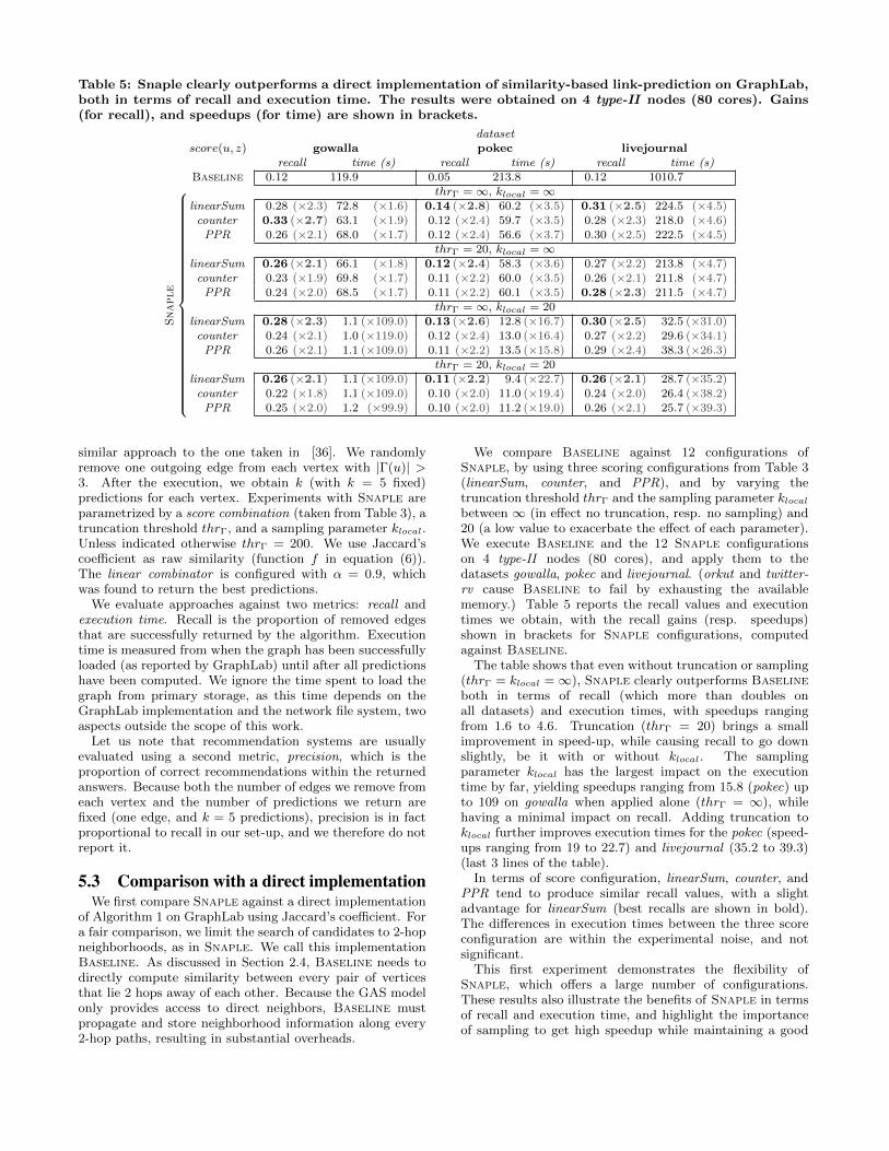
Table 5: Snaple clearly outperforms a direct implementation of similarity-based link-prediction on GraphLab,both in terms of recall and execution time. The results were obtained on 4 type-II nodes (80 cores). Gains(for recall), and speedups (for time) are shown in brackets.
datasetscore(u, z) gowalla pokec livejournal
recall time (s) recall time (s) recall time (s)Baseline 0.12 119.9 0.05 213.8 0.12 1010.7
Snaple
︷︸︸
︷ thrΓ =∞, klocal =∞linearSum 0.28 (×2.3) 72.8 (×1.6) 0.14 (×2.8) 60.2 (×3.5) 0.31 (×2.5) 224.5 (×4.5)counter 0.33 (×2.7) 63.1 (×1.9) 0.12 (×2.4) 59.7 (×3.5) 0.28 (×2.3) 218.0 (×4.6)PPR 0.26 (×2.1) 68.0 (×1.7) 0.12 (×2.4) 56.6 (×3.7) 0.30 (×2.5) 222.5 (×4.5)
thrΓ = 20, klocal =∞linearSum 0.26 (×2.1) 66.1 (×1.8) 0.12 (×2.4) 58.3 (×3.6) 0.27 (×2.2) 213.8 (×4.7)counter 0.23 (×1.9) 69.8 (×1.7) 0.11 (×2.2) 60.0 (×3.5) 0.26 (×2.1) 211.8 (×4.7)PPR 0.24 (×2.0) 68.5 (×1.7) 0.11 (×2.2) 60.1 (×3.5) 0.28 (×2.3) 211.5 (×4.7)
thrΓ =∞, klocal = 20linearSum 0.28 (×2.3) 1.1 (×109.0) 0.13 (×2.6) 12.8 (×16.7) 0.30 (×2.5) 32.5 (×31.0)counter 0.24 (×2.1) 1.0 (×119.0) 0.12 (×2.4) 13.0 (×16.4) 0.27 (×2.2) 29.6 (×34.1)PPR 0.26 (×2.1) 1.1 (×109.0) 0.11 (×2.2) 13.5 (×15.8) 0.29 (×2.4) 38.3 (×26.3)
thrΓ = 20, klocal = 20linearSum 0.26 (×2.1) 1.1 (×109.0) 0.11 (×2.2) 9.4 (×22.7) 0.26 (×2.1) 28.7 (×35.2)counter 0.22 (×1.8) 1.1 (×109.0) 0.10 (×2.0) 11.0 (×19.4) 0.24 (×2.0) 26.4 (×38.2)PPR 0.25 (×2.0) 1.2 (×99.9) 0.10 (×2.0) 11.2 (×19.0) 0.26 (×2.1) 25.7 (×39.3)
similar approach to the one taken in [36]. We randomlyremove one outgoing edge from each vertex with |Γ(u)| >3. After the execution, we obtain k (with k = 5 fixed)predictions for each vertex. Experiments with Snaple areparametrized by a score combination (taken from Table 3), atruncation threshold thrΓ, and a sampling parameter klocal.Unless indicated otherwise thrΓ = 200. We use Jaccard’scoefficient as raw similarity (function f in equation (6)).The linear combinator is configured with α = 0.9, whichwas found to return the best predictions.
We evaluate approaches against two metrics: recall andexecution time. Recall is the proportion of removed edgesthat are successfully returned by the algorithm. Executiontime is measured from when the graph has been successfullyloaded (as reported by GraphLab) until after all predictionshave been computed. We ignore the time spent to load thegraph from primary storage, as this time depends on theGraphLab implementation and the network file system, twoaspects outside the scope of this work.
Let us note that recommendation systems are usuallyevaluated using a second metric, precision, which is theproportion of correct recommendations within the returnedanswers. Because both the number of edges we remove fromeach vertex and the number of predictions we return arefixed (one edge, and k = 5 predictions), precision is in factproportional to recall in our set-up, and we therefore do notreport it.
5.3 Comparison with a direct implementationWe first compare Snaple against a direct implementation
of Algorithm 1 on GraphLab using Jaccard’s coefficient. Fora fair comparison, we limit the search of candidates to 2-hopneighborhoods, as in Snaple. We call this implementationBaseline. As discussed in Section 2.4, Baseline needs todirectly compute similarity between every pair of verticesthat lie 2 hops away of each other. Because the GAS modelonly provides access to direct neighbors, Baseline mustpropagate and store neighborhood information along every2-hop paths, resulting in substantial overheads.
We compare Baseline against 12 configurations ofSnaple, by using three scoring configurations from Table 3(linearSum, counter, and PPR), and by varying thetruncation threshold thrΓ and the sampling parameter klocalbetween ∞ (in effect no truncation, resp. no sampling) and20 (a low value to exacerbate the effect of each parameter).We execute Baseline and the 12 Snaple configurationson 4 type-II nodes (80 cores), and apply them to thedatasets gowalla, pokec and livejournal. (orkut and twitter-rv cause Baseline to fail by exhausting the availablememory.) Table 5 reports the recall values and executiontimes we obtain, with the recall gains (resp. speedups)shown in brackets for Snaple configurations, computedagainst Baseline.
The table shows that even without truncation or sampling(thrΓ = klocal =∞), Snaple clearly outperforms Baselineboth in terms of recall (which more than doubles onall datasets) and execution times, with speedups rangingfrom 1.6 to 4.6. Truncation (thrΓ = 20) brings a smallimprovement in speed-up, while causing recall to go downslightly, be it with or without klocal. The samplingparameter klocal has the largest impact on the executiontime by far, yielding speedups ranging from 15.8 (pokec) upto 109 on gowalla when applied alone (thrΓ = ∞), whilehaving a minimal impact on recall. Adding truncation toklocal further improves execution times for the pokec (speed-ups ranging from 19 to 22.7) and livejournal (35.2 to 39.3)(last 3 lines of the table).
In terms of score configuration, linearSum, counter, andPPR tend to produce similar recall values, with a slightadvantage for linearSum (best recalls are shown in bold).The differences in execution times between the three scoreconfiguration are within the experimental noise, and notsignificant.
This first experiment demonstrates the flexibility ofSnaple, which offers a large number of configurations.These results also illustrate the benefits of Snaple in termsof recall and execution time, and highlight the importanceof sampling to get high speedup while maintaining a good
●
●●
0
250
500
750
68 223 1400Edges in millions
Sec
onds
cores ● 64 128 256
(a) klocal = 40 and type-I
●
●
250
500
750
68 223 1400Edges in millions
Sec
onds
cores ● 64 128 256
(b) klocal = 80 and type-I
●
●
●
100
200
300
400
68 223 1400Edges in millions
Sec
onds
cores ● 80 160
(c) klocal = 40 and type-II
●
●
●
200
400
600
800
68 223 1400Edges in millions
Sec
onds
cores ● 80 160
(d) klocal = 80 and type-II
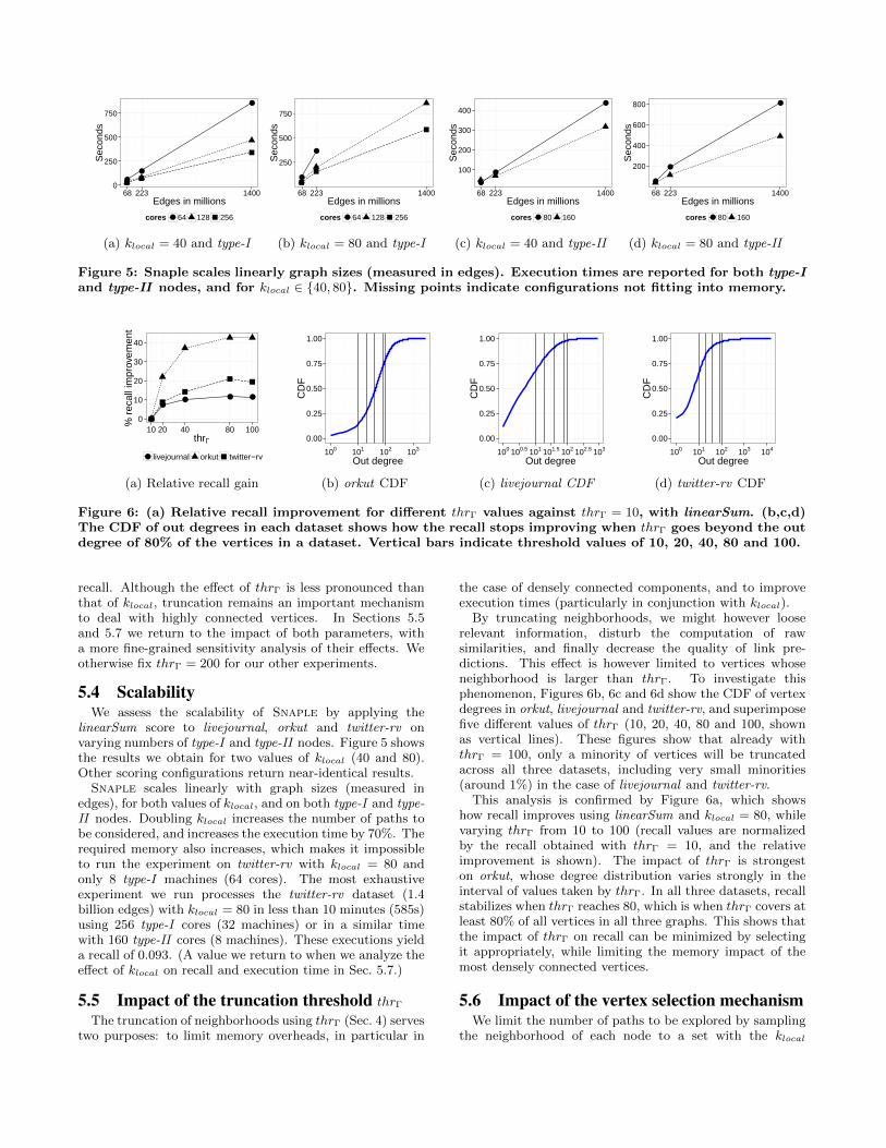
Figure 5: Snaple scales linearly graph sizes (measured in edges). Execution times are reported for both type-Iand type-II nodes, and for klocal ∈ {40, 80}. Missing points indicate configurations not fitting into memory.
●
●●
● ●
0
10
20
30
40
10 20 40 80 100thrΓ
% r
ecal
l im
prov
emen
t
● livejournal orkut twitter−rv
(a) Relative recall gain
0.00
0.25
0.50
0.75
1.00
100 101 102 103
Out degree
CD
F
(b) orkut CDF
0.00
0.25
0.50
0.75
1.00
100 100.5 101 101.5 102 102.5 103
Out degreeC
DF
(c) livejournal CDF
0.00
0.25
0.50
0.75
1.00
100 101 102 103 104
Out degree
CD
F
(d) twitter-rv CDF
Figure 6: (a) Relative recall improvement for different thrΓ values against thrΓ = 10, with linearSum. (b,c,d)The CDF of out degrees in each dataset shows how the recall stops improving when thrΓ goes beyond the outdegree of 80% of the vertices in a dataset. Vertical bars indicate threshold values of 10, 20, 40, 80 and 100.
recall. Although the effect of thrΓ is less pronounced thanthat of klocal, truncation remains an important mechanismto deal with highly connected vertices. In Sections 5.5and 5.7 we return to the impact of both parameters, witha more fine-grained sensitivity analysis of their effects. Weotherwise fix thrΓ = 200 for our other experiments.
5.4 ScalabilityWe assess the scalability of Snaple by applying the
linearSum score to livejournal, orkut and twitter-rv onvarying numbers of type-I and type-II nodes. Figure 5 showsthe results we obtain for two values of klocal (40 and 80).Other scoring configurations return near-identical results.Snaple scales linearly with graph sizes (measured in
edges), for both values of klocal, and on both type-I and type-II nodes. Doubling klocal increases the number of paths tobe considered, and increases the execution time by 70%. Therequired memory also increases, which makes it impossibleto run the experiment on twitter-rv with klocal = 80 andonly 8 type-I machines (64 cores). The most exhaustiveexperiment we run processes the twitter-rv dataset (1.4billion edges) with klocal = 80 in less than 10 minutes (585s)using 256 type-I cores (32 machines) or in a similar timewith 160 type-II cores (8 machines). These executions yielda recall of 0.093. (A value we return to when we analyze theeffect of klocal on recall and execution time in Sec. 5.7.)
5.5 Impact of the truncation threshold thrΓ
The truncation of neighborhoods using thrΓ (Sec. 4) servestwo purposes: to limit memory overheads, in particular in
the case of densely connected components, and to improveexecution times (particularly in conjunction with klocal).
By truncating neighborhoods, we might however looserelevant information, disturb the computation of rawsimilarities, and finally decrease the quality of link pre-dictions. This effect is however limited to vertices whoseneighborhood is larger than thrΓ. To investigate thisphenomenon, Figures 6b, 6c and 6d show the CDF of vertexdegrees in orkut, livejournal and twitter-rv, and superimposefive different values of thrΓ (10, 20, 40, 80 and 100, shownas vertical lines). These figures show that already withthrΓ = 100, only a minority of vertices will be truncatedacross all three datasets, including very small minorities(around 1%) in the case of livejournal and twitter-rv.
This analysis is confirmed by Figure 6a, which showshow recall improves using linearSum and klocal = 80, whilevarying thrΓ from 10 to 100 (recall values are normalizedby the recall obtained with thrΓ = 10, and the relativeimprovement is shown). The impact of thrΓ is strongeston orkut, whose degree distribution varies strongly in theinterval of values taken by thrΓ. In all three datasets, recallstabilizes when thrΓ reaches 80, which is when thrΓ covers atleast 80% of all vertices in all three graphs. This shows thatthe impact of thrΓ on recall can be minimized by selectingit appropriately, while limiting the memory impact of themost densely connected vertices.
5.6 Impact of the vertex selection mechanismWe limit the number of paths to be explored by sampling
the neighborhood of each node to a set with the klocal
●
●●
● ●
●
●● ● ●
●
●● ● ●
counter linearSum PPR
0.10
0.15
0.20
0.25
0.30
5 10 20 40 80 5 10 20 40 80 5 10 20 40 80klocal
Rec
all
● Γklocal
max Γklocal
min Γklocal
rnd
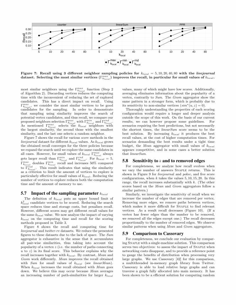
Figure 7: Recall using 3 different neighbor sampling policies for klocal = 5, 10, 20, 40, 80 with the livejournaldataset. Selecting the most similar vertices (Γmaxklocal
) improves the recall, in particular for small values of klocal.
most similar neighbors using the Γmaxklocalfunction (Step 2
of Algorithm 2). Discarding vertices reduces the computingtime with the inconvenient of reducing the set of exploredcandidates. This has a direct impact on recall. UsingΓmaxklocal
, we consider the most similar vertices to be goodcandidates for the sampling. In order to demonstratethat sampling using similarity improves the search ofpotential vertex candidates, and thus recall, we compare ourproposed neighbors selection Γmaxklocal
with Γminklocaland Γrndklocal
.As mentioned Γmaxklocal
selects the klocal neighbors withthe largest similarity, the second those with the smallestsimilarity, and the last one selects a random neighbor.
Figure 7 shows the recall for various score methods in thelivejournal dataset for different klocal values. As klocal growsthe obtained recall converges for the three policies becausewe expand the search until we explore the same candidates inall cases. However, for small values of klocal Γmaxklocal
always
gets larger recall than Γminklocaland Γrndklocal
. For klocal = 5,
Γmaxklocaldoubles Γminklocal
recall and increases 50% compared
to Γrndklocal. This result indicates that using the similarity
as a criterion to limit the amount of vertices to explore isparticularly effective for small values of klocal. Reducing thenumber of vertices to explore reduces both the computationtime and the amount of memory to use.
5.7 Impact of the sampling parameter klocal
The definition of klocal puts an upper bound limit ofk2local candidate vertices to be scored. Reducing the search
space reduces time and storage costs, but penalizes recall.However, different scores may get different recall values forthe same klocal value. We now analyze the impact of varyingklocal on the computing time and recall for the scoringmethods proposed in Table 3.
Figure 8 shows the recall and computing time forlivejournal and twitter-rv datasets. We reduce the presentedfigures to these datasets due to the lack of space. The Sumaggregator is exhaustive in the sense that it accumulatesall pair-wise similarities, thus taking into account thepopularity of a vertex z (i.e. the number of paths connectingu to z) in its final score. This behavior explains why therecall increases together with klocal. By contrast, Mean andGeom work differently. Mean improves the recall obtainedwith Sum for small values of klocal (see linearMean).When klocal increases the recall obtained with Mean goesdown. We believe this may occur because Mean averagesan increasing number of path-similarities for larger klocal
values, many of which might have low scores. Additionally,averaging eliminates information about the popularity of avertex, contrarily to Sum. The Geom aggregator show thesame pattern in a stronger form, which is probably due toits sensitivity to non-similar vertices (sim?(u, z) = 0).
Thoroughly understanding the properties of each scoringconfiguration would require a longer and deeper analysisoutside the scope of this work. On the basis of our currentresults, we can however propose some guidelines. Forscenarios requiring the best predictions, but not necessarilythe shortest times, the linearSum score seems to be thebest solution. By increasing klocal it produces the bestrecall values, at the cost of higher computation times. Forscenarios demanding the best results under a tight timebudget, the Mean aggregator with small values of klocalappears competitive, and in some cases a better solutionthat linearSum.
5.8 Sensitivity to k and to removed edgesFor completeness, we analyze how recall evolves when
we vary the number of answers Snaple returns. This isshown in Figure 9 for livejournal and pokec, and five scoreconfigurations, when k takes the values 5, 10, 15, 20. In thisrange, the recall increases substantially with k. (The otherscores based on the Mean and Geom aggregators follow asimilar pattern.)
Similarly, we investigate the sensitivity of recall when weincrease the number of edges that are removed per vertex.Removing more edges, we remove paths between vertices,which makes it more difficult for Snaple to find relevantvertices. As a result recall decreases (Figure 10). (If avertex has fewer edges than the number to be removed,we removed all the edges except one.) The recall decreasesproportionally to the number of removed edges. We observesimilar patterns when using Mean and Geom aggregators.
5.9 Comparison to CassovaryFor completeness, we conclude our evaluation by compar-
ing Snaple with a single-machine solution. This comparisonserves two objectives: to assess the impact of Snaple whennetworking costs disappear, and to provide a reference pointto gauge the benefits of distribution when processing verylarge graphs. We use Cassovary [42] for this comparison,a multithreaded in-memory graph library from Twitter.Cassovary is able to load relative large graphs and cantraverse a graph fully allocated into main memory. It hasbeen shown to be a efficient solution for computing random

●
●
●
●●
0.225
0.250
0.275
0.300
0.325
15 20 25 30 35 40Seconds
Rec
all
● countereuclSum
geomSumlinearSum
PPR
●
●
●
●●
0.05
0.06
0.07
0.08
0.09
200 300 400 500 600Seconds
Rec
all
● countereuclSum
geomSumlinearSum
PPR
(a) Sum aggregator for livejournal (left) and twitter-rv (right)
●
●
●
●●
0.19
0.20
0.21
0.22
0.23
15 20 25 30 35 40Seconds
Rec
all
● euclMeangeomMean
linearMean
●
●
●
●
●0.04
0.05
0.06
200 300 400 500 600Seconds
Rec
all
● euclMeangeomMean
linearMean
(b) Mean aggregator for livejournal (left) and twitter-rv (right)
●
●
● ●
0.100
0.125
0.150
0.175
15 20 25 30 35 40Seconds
Rec
all
● euclGeomgeomGeom
linearGeom
●
●
●
●
●
0.02
0.03
0.04
0.05
0.06
200 300 400 500 600Seconds
Rec
all
● euclGeomgeomGeom
linearGeom
(c) Geom aggregator for livejournal (left) and twitter-rv (right)
Figure 8: Comparison of computing time againstrecall for different scoring configurations on 256cores. Each point corresponds to a different value ofklocal = 5, 10, 20, 40, 80. The sum aggregator gets thehighest recall, improving as klocal grows.
walks [19, 24]. It is also used in production by Twitter [12].In a first attempt, we implemented the solution described
by Algorithm 1 (with the 2-hop optimization). However,neither the recall nor computing time were competitive.We therefore moved on to a multithreaded version of thepersonalized page rank (PPR) [30] approximation based onrandom walks [37] to improve on these results. For eachvertex we run w random walks of depth d. d = 2 reaches theneighbors of a vertex ; d = 3 its neighbors of neighbors andso on. Once the random walks terminates, the k most visitedvertices not included into Γ(v) are returned as predictions.Increasing w and d, we force the algorithm to explore a largernumber of vertices in a similar way we do when varyingklocal. We modify w and d configurations in order to findthe largest recall in the shortest time.
Figure 11 compares the recall and computing time forCassovary running on a type-II machine when varying w and
●
●
●
●
0.30
0.35
0.40
0.45
5 10 15 20k
Rec
all
● countereuclSum
geomSumlinearSum
PPR
(a) livejournal
●
●
●
●
0.125
0.150
0.175
0.200
0.225
5 10 15 20k
Rec
all
● countereuclSum
geomSumlinearSum
PPR
(b) pokec
Figure 9: Evolution of recall when increasing thenumber of recommended links k with klocal = 80.
●
●
●
●
●
0.21
0.24
0.27
0.30
1 2 3 4 5Removed edges vertex
Rec
all
● countereuclSum
geomSumlinearSum
PPR
(a) livejournal
●
●
●●
●
0.08
0.10
0.12
0.14
1 2 3 4 5Removed edges vertex
Rec
all
● countereuclSum
geomSumlinearSum
PPR
(b) pokec
Figure 10: Evolution of recall when increasing thenumber of removed edges per vertex with klocal = 80.
●
●
●
w = 100
0.05
0.10
0.15
0.20
0.25
50 100 150 200 250Seconds
Rec
all
● PPR d=10PPR d=3
PPR d=4PPR d=5
(a) livejournal
●
●w = 1000
0.02
0.03
0.04
0.05
0.06
2000 4000 6000Seconds
Rec
all
● PPR d=10PPR d=3
PPR d=4PPR d=5
(b) twitter-rv
Figure 11: Recall and computing time using a stand-alone link-prediction solution on top of Cassovaryusing random walks to emulate PPR. Both solutionsare run on a type-II machine with w = 10, 100, 1000.
d on the livejournal and twitter-rv datasets. We observe thatincreasing d does not necessarily improve recall, with d = 3yielding recall values very close to that of larger values of d.By contrast, larger values of w tend to yield better recallvalue, but they also significantly increase the computingtime. In the case of twitter-rv, we run an extra configurationwith d = 3 and w = 10000 getting 0.06 recall in 90 minutes.Unfortunately, we had to stop other configurations withlarger d values and w = 10000 as they took too long tocomplete.
Snaple is designed to run on a distributed environment
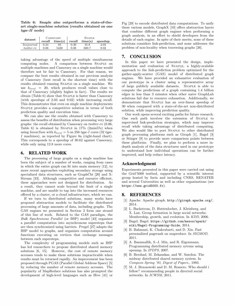
Table 6: Snaple also outperforms a state-of-the-art single-machine solution (results obtained on onetype-II node)
datasetCassovary Snaple
recall time(s) recall time(s) speeduplivejournal 0.24 93 0.30 45.8 2.03twitter-rv 0.06 5420 0.08 600.7 9.02
taking advantage of the speed of multiple simultaneouscomputing nodes. A comparison between Snaple onmultiple machines and Cassovary on a single machine wouldtherefore not be fair to Cassovary. For that reason, wecompare the best results obtained in our previous analysisof Cassovary (best recall in the shortest time) with theresults obtained running Snaple on a single machine. Weuse klocal = 20, which produces recall values close tothat of Cassovary (slightly higher in fact). The results weobtain (Table 6) show that Snaple is faster than Cassovary(with speedups of 2.03 and 9.02) while increasing recall.This demonstrates that even on single machine deploymentsSnaple provides a competitive solution in terms of bothprediction quality and execution time.
We can also use the results obtained with Cassovary toassess the benefits of distribution when processing very largegraphs: the recall obtained by Cassovary on twitter-rv (0.06,Table 6) is obtained by Snaple in 177s (2min57s) whenusing linearSum with klocal = 5 on 256 type-I cores (32 type-I machines), as reported by Figure 8a (right-hand chart).This corresponds to a speedup of 30.62 against Cassovary,while only using 12.8 more cores.
6. RELATED WORKThe processing of large graphs on a single machine has
been the subject of a number of works, ranging from casesin which the entire graph can fit into main memory [12], tomore recent approaches exploiting secondary storage usingspecialized data structures, such as GraphChi [20] and X-Stream [33]. Although competitive and resource efficient,these approaches were not designed for distribution. Asa result, they cannot scale beyond the limit of a singlemachine, and are unable to tap into the increased resourcesoffered by a cluster, or a cloud infrastructure, which we can.
If we turn to distributed solutions, many works haveproposed abstraction models to facilitate the distributedprocessing of large amounts of data, including graphs. TheGAS engines we presented in Section 2 form one strandof this line of work. Related to the GAS paradigm, theBulk Synchronous Parallel (or BSP) model [43] organizesa parallel computation into asynchronous supersteps thatare then synchronized using barriers. Pregel [27] adapts theBSP model to graphs, and organizes computation aroundfunctions executing on vertices that exchange messagesbetween each supersteps.
The complexity of programming models such as BSPhas led researchers to propose distributed shared memorysolutions [6, 15]. However, the cost of remote memoryaccesses tends to make these solutions impracticable whenresults must be returned rapidly. An improvement has beenproposed through PGAS (Parallel Global Address Space) [5]by reducing the number of remote memory accesses. Thepopularity of MapReduce solutions has also prompted thedevelopment of high-level languages such as Hive [41] or
Pig [29] to encode distributed data computations. To unifythese various models, GraphX [10] offers abstraction layersthat combine different graph engines when performing agraph analysis, in an effort to shield developers from thedetails of each engine. In spite of their merits, none of thesesolutions considers link-prediction, and none addresses theproblem of non-locality when traversing graphs [26].
7. CONCLUSIONIn this paper we have presented the design, imple-
mentation and evaluation of Snaple, a highly-scalableapproach to the link-prediction problem optimized for thegather-apply-scatter (GAS) model of distributed graphengines. We have provided an exhaustive evaluation ofour prototype in a cluster using a representative arrayof large publicly available datasets. Snaple is able tocompute the predictions of a graph containing 1.4 billionedges in less than 3 minutes when other naive GraphLabsolutions fail due to resource exhaustion. Additionally, wedemonstrate that Snaple has an over-linear speedup of30 when compared with a state-of-the-art non-distributedsolution, while improving prediction quality.
Our work opens several exciting paths for future research.One such path involves the extension of Snaple tosupervised link-prediction strategies, which may improverecall while taking advantage of distributed computing.We also would like to port Snaple to other distributedgraph processing platforms such as Giraph [1], Bagel [3]or Stinger [9] to provide more comparison points betweenthese platforms. Finally, we plan to perform a more in-depth analysis of the data structures used in our prototypeto understand how individual operations can be furtherimproved, and help reduce latency.
AcknowledgmentExperiments presented in this paper were carried out usingthe Grid’5000 testbed, supported by a scientific interestgroup hosted by Inria and including CNRS, RENATERand several Universities as well as other organizations (seehttps://www.grid5000.fr).
8. REFERENCES[1] Apache. Apache giraph. http://giraph.apache.org/,
2014.
[2] L. Backstrom, D. Huttenlocher, J. Kleinberg, andX. Lan. Group formation in large social networks:Membership, growth, and evolution. In KDD, 2006.
[3] Bagel. Bagel. https://github.com/mesos/spark/wiki/Bagel-Programming-Guide, 2014.
[4] B. Bahmani, K. Chakrabarti, and D. Xin. Fastpersonalized pagerank on mapreduce. In SIGMOD,2011.
[5] A. Basumallik, S.-J. Min, and R. Eigenmann.Programming distributed memory sytems usingopenmp. In IPDPS, 2007.
[6] B. Bershad, M. Zekauskas, and W. Sawdon. Themidway distributed shared memory system. InCompcon Spring ’93, Digest of Papers., 1993.
[7] M. J. Brzozowski and D. M. Romero. Who should ifollow? recommending people in directed socialnetworks. In ICWSM, 2011.
[8] E. Cho, S. A. Myers, and J. Leskovec. Friendship andmobility: User movement in location-based socialnetworks. In KDD, 2011.
[9] D. Ediger, R. McColl, E. J. Riedy, and D. A. Bader.Stinger: High performance data structure forstreaming graphs. In HPEC, 2012.
[10] J. Gonzalez, R. Xin, A. Dave, D. Crankshaw,M. Franklin, and I. Stoica. Graphx: Graph processingin a distributed dataflow framework. In OSDI, 2014.
[11] J. E. Gonzalez, Y. Low, H. Gu, D. Bickson, andC. Guestrin. Powergraph: Distributed graph-parallelcomputation on natural graphs. In OSDI, 2012.
[12] P. Gupta, A. Goel, J. Lin, A. Sharma, D. Wang, andR. Zadeh. WTF: the who to follow service at twitter.In WWW, pages 505–514, 2013.
[13] M. Han, K. Daudjee, K. Ammar, M. T. Ozsu,X. Wang, and T. Jin. An experimental comparison ofpregel-like graph processing systems. Proceedings ofthe VLDB Endowment, 7(12), 2014.
[14] M. Hasan and M. Zaki. A survey of link prediction insocial networks. In C. C. Aggarwal, editor, SocialNetwork Data Analytics, pages 243–275. Springer US,2011.
[15] K. L. Johnson, M. F. Kaashoek, and D. A. Wallach.Crl: High-performance all-software distributed sharedmemory. SIGOPS Oper. Syst. Rev., 1995.
[16] A.-M. Kermarrec, F. Taıani, and J. M. Tirado. Cheapand cheerful: Trading speed and quality for scalablesocial-recommenders. In DAIS, 2015.
[17] Z. Khayyat, K. Awara, A. Alonazi, H. Jamjoom,D. Williams, and P. Kalnis. Mizan: a system fordynamic load balancing in large-scale graphprocessing. In Eurosys, 2013.
[18] H. Kwak, C. Lee, H. Park, and S. Moon. What istwitter, a social network or a news media? In WWW,2010.
[19] A. Kyrola. Drunkardmob: Billions of random walks onjust a pc. In RecSys, 2013.
[20] A. Kyrola, G. Blelloch, and C. Guestrin. Graphchi:Large-scale graph computation on just a pc. In OSDI,2012.
[21] R. Lempel and S. Moran. The stochastic approach forlink-structure analysis (salsa) and the tkc effect.Comput. Netw., 33(1-6):387–401, June 2000.
[22] D. Liben-Nowell and J. Kleinberg. The link predictionproblem for social networks. In CIKM, 2003.
[23] R. N. Lichtenwalter, J. T. Lussier, and N. V. Chawla.New perspectives and methods in link prediction. InKDD, 2010.
[24] P. A. Lofgren, S. Banerjee, A. Goel, and C. Seshadhri.Fast-ppr: Scaling personalized pagerank estimation forlarge graphs. In KDD, 2014.
[25] Y. Low, D. Bickson, J. Gonzalez, C. Guestrin,A. Kyrola, and J. M. Hellerstein. Distributedgraphlab: A framework for machine learning and datamining in the cloud. Proc. VLDB Endow., 2012.
[26] A. Lumsdaine, D. Gregor, B. Hendrickson, and J. W.Berry. Challenges in parallel graph processing. ParallelProcessing Letters, 17(1):5–20, 2007.
[27] G. Malewicz, M. H. Austern, A. J. Bik, J. C. Dehnert,I. Horn, N. Leiser, and G. Czajkowski. Pregel: A
system for large-scale graph processing. In SIGMOD,2010.
[28] A. Mislove, M. Marcon, K. P. Gummadi, P. Druschel,and B. Bhattacharjee. Measurement and Analysis ofOnline Social Networks. In IMC, 2007.
[29] C. Olston, B. Reed, U. Srivastava, R. Kumar, andA. Tomkins. Pig latin: A not-so-foreign language fordata processing. In Proceedings of the 2008 ACMSIGMOD International Conference on Management ofData, SIGMOD ’08, pages 1099–1110, 2008.
[30] L. Page, S. Brin, R. Motwani, and T. Winograd. Thepagerank citation ranking: Bringing order to the web.Technical Report 1999-66, Stanford InfoLab,November 1999.
[31] R. Parimi and D. Caragea. Predicting friendship linksin social networks using a topic modeling approach. InPAKDD, 2011.
[32] M. Rowe, M. Stankovic, and H. Alani. Who will followwhom? exploiting semantics for link prediction inattention-information networks. In ISWC, 2012.
[33] A. Roy, I. Mihailovic, and W. Zwaenepoel. X-stream:Edge-centric graph processing using streamingpartitions. In SOSP, 2013.
[34] S. Salihoglu and J. Widom. Gps: A graph processingsystem. In SSDBM, page 22. ACM, 2013.
[35] G. Salton and M. J. McGill. Introduction to ModernInformation Retrieval. McGraw-Hill, 1986.
[36] P. Sarkar and A. W. Moore. Fast nearest-neighborsearch in disk-resident graphs. In KDD, 2010.
[37] T. Sarlos, A. A. Benczur, K. Csalogany, D. Fogaras,and B. Racz. To randomize or not to randomize:Space optimal summaries for hyperlink analysis. InWWW, 2006.
[38] S. Scellato, A. Noulas, and C. Mascolo. Exploitingplace features in link prediction on location-basedsocial networks. In KDD, 2011.
[39] R. Schifanella, A. Barrat, C. Cattuto, B. Markines,and F. Menczer. Folks in folksonomies: social linkprediction from shared metadata. In WSDM, 2010.
[40] L. Takac and M. Zabovsky. Data analysis in publicsocial networks. In Int. Science Conf. and Int.Workshop Present Day Trends of Innovation, 2012.
[41] A. Thusoo, J. S. Sarma, N. Jain, Z. Shao, P. Chakka,S. Anthony, H. Liu, P. Wyckoff, and R. Murthy. Hive:A warehousing solution over a map-reduce framework.Proc. VLDB Endow., 2(2):1626–1629, Aug. 2009.
[42] Twitter. Cassovary.https://github.com/twitter/cassovary, 2014.
[43] L. G. Valiant. A bridging model for parallelcomputation. Commun. ACM, 1990.
[44] D. Yin, L. Hong, and B. D. Davison. Structural linkanalysis and prediction in microblogs. In CIKM, 2011.