HAL Id: hal-02398469https://hal-centralesupelec.archives-ouvertes.fr/hal-02398469

Submitted on 2 Mar 2020

HAL is a multi-disciplinary open accessarchive for the deposit and dissemination of sci-entific research documents, whether they are pub-lished or not. The documents may come fromteaching and research institutions in France orabroad, or from public or private research centers.

L’archive ouverte pluridisciplinaire HAL, estdestinée au dépôt et à la diffusion de documentsscientifiques de niveau recherche, publiés ou non,émanant des établissements d’enseignement et derecherche français ou étrangers, des laboratoirespublics ou privés.

Scaling of heated plane jets with moderate radiativeheat transfer in coupled DNS

J. M. Armengol, Ronan Vicquelin, Axel Coussement, R. G. Santos, OlivierGicquel

To cite this version:J. M. Armengol, Ronan Vicquelin, Axel Coussement, R. G. Santos, Olivier Gicquel. Scaling ofheated plane jets with moderate radiative heat transfer in coupled DNS. International Journal ofHeat and Mass Transfer, Elsevier, 2019, 139, pp.456-474. 10.1016/j.ijheatmasstransfer.2019.05.025.hal-02398469

Scaling of heated plane jets with moderate radiative heat transfer in coupled DNS

J.M. Armengola,c,∗, R. Vicquelina, A. Coussementb, R.G. Santosc, O. Gicquela

aLaboratoire EM2C, CNRS, CentraleSupelec, Universite Paris-Saclay, Gif-sur-Yvette, FrancebAero-Thermo-Mechanics Laboratory, Ecole Polytechnique de Bruxelles, Universite Libre de Bruxelles, Bruxelles, Belgium

cFaculty of Mechanical Engineering, University of Campinas (UNICAMP), Campinas-SP, Brazil5

Abstract

The effects of thermal radiation in a heated jet of water vapor are studied with a direct numerical simulation coupled

to a Monte-Carlo solver. The adequacy of the numerical setup is first demonstrated in the uncoupled isothermal

and heated turbulent plane jets with comparisons to experimental and numerical data. Radiative energy transfer is

then accounted for with spectral dependency of the radiative properties described by the Correlated-k (ck) method.10

Between the direct impact through modification of the temperature field by the additional radiative transfer and the

indirect one where the varied flow density changes the turbulent mixing, the present study is able to clearly identify

the second one in the jet developed region by considering conditions where effects of thermal radiation are moderate.

When using standard jet scaling laws, the different studied cases without radiation and with small-to-moderate

radiative heat transfer yield different profiles even when thermal radiation becomes locally negligible. By deriving15

another scaling law for the decay of the temperature profile, self-similarity is obtained for the different turbulent

jets. The results of the study allow for distinguishing whether thermal radiation modifies the nature of heat transfer

mechanisms in the jet developed region or not while removing the indirect effects of modified density.

Keywords: Turbulent jet; Scaling; Direct Numerical Simulation; Thermal radiation; Monte-Carlo

method20

1. Introduction

Free shear flows compound an important branch of turbulent flows, its fundamental understanding is necessary to

comprehend and to predict the transport processes in many industrial applications such as combustion, propulsion and

environmental flows. Greats efforts have been made to describe the dynamics of these flows at the developed region

where turbulent statistics are assumed independent of initial conditions and present universal similarity solutions25

[1–4].

Early similarity solutions of the velocity field based on local velocity and length scales for constant-density free

shear flows are derived in the work of Townsend [2]. Following this work, self-similarity on a constant density

plane jet was reported in the experimental studies of Bradbury [5] and Heskestad [6] using hot-wire anemometry.

They collected data of mean velocity, turbulent intensities and shear stresses fields, as well as the turbulent kinetic30

energy balance in the developed region. Further experimental work was conducted by Gutmark and Wygnanski [7]

applying conditional sampling techniques in order to provide data obtained exclusively within the turbulent zone.

Despite some scatter among these experimental works ([5–7]), data of the velocity field was found to be self-similar

in the developed region when scaled using the classical parameters of Townsend [2]. More recent experimental works

∗Corresponding authorEmail address: jan@fem.unicamp.br (J.M. Armengol)

Preprint submitted to International Journal of Heat and Mass Transfer February 29, 2020

performed by Deo et al. [8, 9] underline the influence of the Reynolds number and the nozzle-exit geometric profile35

on self-similar solution of a plane jet. Accurate data of the constant-density plane jet has also been provided by

numerical investigations including the work of Le Ribault et al. [10] using Large Eddy Simulations (LES) and Stanley

et al. [11] through Direct Numerical Simulations (DNS). Both works obtained similarity profiles for mean velocity

and Reynolds stresses. Proceeding with these studies, Klein et al. [12] numerically investigated the influence of the

Reynolds number and the inflow conditions in a constant-density plane jet using DNS. A recent study of Sadeghi et40

al. [13] proposes new scaling laws for the higher moments in constant-density temporally evolving plane jet which

were derived using Lie symmetry analysis.

For the constant-density round jets, the numerical work of Bogey and Bailly [14] report reference solutions in the

self-preserving region including the turbulence and energy budgets. Further similarity analysis in round jets include

the theoretical and experimental work of Sadeghi et al. [15] who derived a similarity law for the turbulent energy45

structure function; and the work of Thiesset et al. [16] who discussed the similarity of the mean kinetic energy

dissipation rate, and pointed out that assuming local isotropy and complete self-similarity, as well as considering

only production and advection in the energy budget, the virtual origin in one configuration should be the same

independently of the flow quantity under consideration.

Variable-density free shear flows, as opposed to the constant-density ones, have received less attention despite its50

broad engineering importance associated with the mixing process. For the case of free jets, initial density differences

are typically imposed by jet gas composition or by heating the jet fluid. The work of Chen and Rodi [17] showed

that when jet and ambient densities differ significantly self-similarity is not achieved. Nevertheless, for a sufficient

distance downstream, density gradients across the flow decreases and thus the solution asymptotically approaches

self-similarity if scaled by an effective radius which compensates the effects of density as explained in the work of55

Thring and Newby [18]. Richards and Pitts [19] experimentally investigated variable-density axisymmetric jets with

density ratio between 0.138 and 1.552. They analyzed data from downstream distances at which the local density

ratio of the jet to ambient fluid approached unity achieving to characterize the self-similar solution of both mean and

fluctuations values of a passive scalar field. Experimental works of Jenkins and Goldschmidt [20], Davies et al. [21]

and Antonia et al. [22] addressed the variable-density plane jet considering slightly heated jets with density ratios60

between 0.8 and 0.9, i.e., temperature is considered as a passive scalar causing little effects on the evolution of the

flow field. They found similarity profiles of temperature using the classical scaling law since density gradients were

low. All these authors [20–22] found that the spreading rate based on temperature is larger than the one based on

velocity. The stability of variable-density plane jets has been experimentally studied by Yu et al. [23] for density

ratio between 0.73 and 1, and Raynal et al. [24] within a range for the density ratio of 0.14 - 1. They found that the65

oscillating regime disappears above a critical value of the density ratio which increases with the Reynolds number.

The interaction of turbulent flows and thermal radiation has been reviewed in detail in the studies of Coelho

[25], and Modest and Haworth [26]. Several works have quantified turbulence effects on radiation (the so-called TRI)

through uncoupled computations and a priori analysis in a variety of configurations such as turbulent diffusion jet

flames [27], homogeneous isotropic turbulence [28–31], and temporally evolving jet [32]. Coupled simulations solving70

both fluid dynamics and radiation allow for capturing these interactions, as well as radiation effects on turbulence,

although additional modeling can be necessary depending on the turbulence description. Early coupled simulations

2

using Reynolds average Navier-Stokes (RANS) include the studies of diffusion jet flames of Tesse et al. [33] who

pointed out the important role of soot particles in global radiative loss; and the work of Li and Modest [34] in which

was found that TRI reduces the total drop in flame peak temperature caused by radiative heat losses. Additionally, a75

recent RANS coupled simulation in a high-pressure gas turbine combustion chamber was reported by Ren et al. [35].

In the coupled LES framework, Gupta et al. [36] characterized contributions of subfilter-scale fluctuations to TRI in

a diffusion flame; Ghosh et al. [37] observed that radiation counteract the effects of compressibility in a nonreactive

supersonic channel flow; and Poitou et al. [38] showed how radiation can change the flame brush structure. Still in

the LES formulation, coupled simulations in complex geometries of combustion chambers include the works of Jones80

and Paul [39], Berger et al. [40], and Koren et al. [41]. Several coupled DNS works, for which all interactions are fully

captured, have been performed on different systems: statistically 1-dimensional premixed [42, 43] and nonpremixed

[44] flames; natural convection in a differentially heated cubical cavity [45]; and nonreactive channel flow [46, 47];

leading to an understanding of the mechanisms in which radiation modifies turbulence, and a direct quantification

of TRI.85

Given the complexity of combustion systems, it is desirable to simplify the problem by considering non-reactive

free shear flows to understand the isolated impact of radiation in a more canonical configuration without wall

interactions. With the exception of the LES study of Ghosh et al. [48], most coupled works addressing free shear

flows problems correspond however to combustion systems. The effects of thermal radiation in nonreactive turbulent

jets deserves then further investigation. As far as we know, the present set of simulations are the first DNS of a free90

shear flow to be fully coupled with a spectral radiative heat transfer solver.

Radiative heat transfer can modify the jet scaling laws in two ways: first, a different nature and balance of the

different heat transfer mechanisms, and secondly a variation in density due to the modified temperature field. In

order to fully characterize the first phenomenon of high interest, it is necessary to establish scaling laws that can

distinguish both mechanisms. The present study aims then at analyzing the scaling laws of turbulent heated jets95

without radiation and with moderate radiative transfer to consider mainly the second mechanism. The results will

indeed show that moderate radiation effects can change the classical jet scaling laws in the developed region although

thermal radiation can be locally negligible in this region. Without any adaptation of the jet scaling laws for variable

density, one wrongly concludes about the modified balance of heat transfers in the studied case. The paper considers

then another set of scaling laws and derives a new one for the mean temperature field in particular to make cases100

without radiation and with small-to-moderate radiative effects self-similar. These results allow for a future clear

identification of changes in the nature of heat transfer mechanisms due to radiation whether its magnitude is small,

moderate or large.

In the considered case, a heated water vapor mixture discharges into a parallel low-speed coflow of cold water

vapor. The numerical study is carried out with state-of-the-art fidelity to be as representative as possible of an actual105

jet in a participating medium. The turbulent jet is described by a DNS coupled to a reciprocal Monte-Carlo method

to solve the radiative transfer equation. The spectral dependency of the radiative properties is accounted for with

an accurate ck method.

The studied configuration and the adopted numerical methodology are described in §2. A detailed validation

of the isothermal and heated plane jets without radiation is then presented in §3. Finally, results of the heated jet110

3

coupled with thermal radiation are analyzed in §4 using both the classical adimensionalization and a new scaling for

the mean temperature decay.

2. Models and numerical approaches

2.1. Physical case: the plane jet

The present work studies the radiative transfer in a heated turbulent plane jet of water vapor discharging into115

a parallel low speed coflow of cold water vapor. The principal direction of the mean flow is x, the cross-stream

coordinate is y, and z is the spanwise coordinate for which all the statistics are homogeneous. There is statistical

symmetry about the plane y = 0. The flow statistics are stationary and two-dimensional. Figure 1 shows a schematic

representation in which the jet mixes with the surrounding slow coflow, which creates turbulence and increases the

jet thickness.120

zx

y

dDUc

Initial zone Fully turbulent jet flow

y1/2Heated Jet U1 T1

Cold CoflowU2 T2

DUc/2

Figure 1: Schematic representation of the turbulent structures of a heated plane jet identified by the Q-criterion.

At the inlet boundary, the jet width opening is set to δ = 0.05 m. Computations are performed in a domain

extension of 13.5δ×10δ×3δ in x, y and z directions, respectively, while mean results are computed in a 10δ×10δ×3δ

box. The jet has an initial mean velocity U1 = 4.176 m/s and the mean coflow velocity is set to U2 = U1/10. The jet

temperature is fixed to T1 = 860 K, while the temperature in the coflow is T2 = 380 K, this temperature range has

been chosen based on typical values found in a steam turbine [49]. All simulations are carried out at atmospheric125

pressure (1 atm).

The corresponding Reynolds number based on the width opening δ is

Re =ρ(T1)∆U0δ

µ(T1)= 1500, (1)

where ∆U0 = U1 − U2. This Reynolds number is moderate compared with previous DNS studies of the turbulent

plane jet. For example, Klein et al. [12] investigated the influence of the Reynolds number in the range of 1000 to

6000, and Stanley et al. [11] simulated the plane jet using a Reynolds number of 3000. In our study, the Reynolds130

number is kept moderate in order to afford the computational cost of a coupled simulation with thermal radiation

4

while featuring a fully turbulent flow as seen in Fig. 1. The half width of the jet y1/2(x) displayed in Fig. 1 is a mean

quantity useful to describe the jet spreading rate. It is defined as the distance from the jet centerline at which the

mean velocity corrected by the coflow velocity is half of the value at the jet centerline. In the isothermal turbulent

plane jet, the local Reynolds number based on y1/2 and the jet centerline velocity grows downstream in the fully135

turbulent region as x1/2.

Experimental studies of the plane jet show that mean turbulent fields can be divided into two distinct regions

along the x direction [1]. The first region is the initial zone located in the vicinity of the nozzle. In this region the

jet is surrounded by a mixing layer on top and bottom, and turbulence penetrates inwards toward the centerline of

the jet. Until the growth of these mixing layers does not reach the jet centerline, there is a region called potential140

core, unaffected by the turbulence from these shear layers. In the potential core, the injected hot mixture remains

uniform. The length of the initial zone is strongly affected by the inlet conditions as reported by experimental [9]

and numerical [12] studies. In the second region, called fully turbulent, turbulence has penetrated into the centerline

of the jet and the mean streamwise velocity profile has a rounded shape. In this region, the mean fields of the

isothermal plane jet become self-similar.145

2.2. Flow simulation

2.2.1. Governing equations

The governing equations used to describe the dynamics of the plane jet are the Navier-Stokes equations for a

compressible fluid. These are the continuity equation, the momentum and energy transport equations, respectively:

∂ρ

∂t+∂ (ρui)

∂xi= 0, (2)

∂ρuj∂t

+∂ (ρuiuj)

∂xi= − ∂p

∂xj+∂τij∂xi

, (3)

∂ρet∂t

+∂ (ρetui)

∂xi= −∂(puj)

∂xj+∂(τijui)

∂xj+

∂

∂xi

(λ∂T

∂xi

)+ Prad, (4)

where ρ, t, uj , p, τij , et, λ and T denote density, time, instantaneous velocity, pressure, stress tensor, total energy,150

thermal conductivity and temperature, respectively. The mixture is homogeneous and made of pure water vapor.

Prad is the radiative power further discussed in § 2.2.3. Assuming Newtonian fluid, the stress tensor τi,j is defined as

τij = µ

((∂ui∂xj

+∂uj∂xi

)− 2

3δij∂uk∂xk

), (5)

where µ is the dynamic viscosity and δij is the Kronecker delta operator. The energy transport is defined based

on the total energy et, which accounts for the sum of internal and kinetic energies: et = 12uiui + e, where e is the

internal energy. The enthalpy is denoted by h = e + rT where r = R/W and R is the universal gas constant. W155

stands for the molar weight of the mixture which is here pure water vapor.

The ideal gas equation is used to compute the pressure as

p = ρrT. (6)

5

Computation of the transport properties of water vapor is based on the data of Lemmon et al. [50]. Heat capacity

at constant pressure is assumed constant since it varies less than 6.4% in the considered temperature range, while µ

and λ vary around 163 % and 205%, respectively [50]. A polynomial regression of order two is then carried out in160

order to approximate the dynamic viscosity µ and thermal conductivity λ as follows

µ(T ) = a0 + a1

(T

Tref

)+ a2

(T

Tref

)2

, and λ(T ) = b0 + b1

(T

Tref

)+ b2

(T

Tref

)2

, (7)

where T is in Kelvin, Tref is a reference temperature Tref = 400 K, a0 = −5.9340 × 10−6Pa · s, a1 = 1.9303 ×

10−5Pa · s and a2 = −7.4821 × 10−7Pa · s, b0 = 5.0855 × 10−3W/(m · K), b1 = 1.5698 × 10−2W/(m · K) and

b2 = 8.5830× 10−3W/(m ·K).

2.2.2. Numerical techniques165

The governing equations are numerically solved on a structured mesh using a 4th-order centered finite-difference

scheme for the spatial derivatives and an explicit 4th-order Runge-Kutta method for the time integration, an overview

of such methods can be found in the work of Kennedy and Carpenter [51]. In addition, an implicit filter of 8th-order

proposed in the work of Gaitonde and Visbal [52] is used for stability purposes.

Boundary conditions treatment. Boundary conditions are treated with the 3D Navier-Stokes Characteristic170

Boundary Conditions method as described in the work of Coussement et al. [53]. Specifications of the boundary

conditions and the computation domain are presented in Fig. 2. In the outflow boundaries, atmospheric pressure is

enforced with a partially reflecting characteristic boundary condition.

Ly

Lx

Lzy

z x

Figure 2: Schematic representation of boundary conditions in a snapshot of turbulent eddies identified by the Q-criterion coloured by

temperature.

6

The inlet mean streamwise velocity profile Uin that defines the jet is specified by the hyperbolic function:

Uin(y) =U1 + U2

2+U1 − U2

2tanh

(δ/2− |y|

2θ

), (8)

where θ is the shear layer momentum thickness set to θ = 0.07δ. Those values are similar to a previous work of a175

DNS plane jet [11]. Low values of the shear layer momentum thickness promote the jet growth but required more

mesh refinement to well describe the velocity gradients in the jet edge.

The Reynolds averaging and the time Favre averaging operations for any variable φ are here defined as 〈φ〉 and

φ, while φ′ and φ′′ denote their respective fluctuating parts. Then, the Favre averaged velocity profile at the inlet

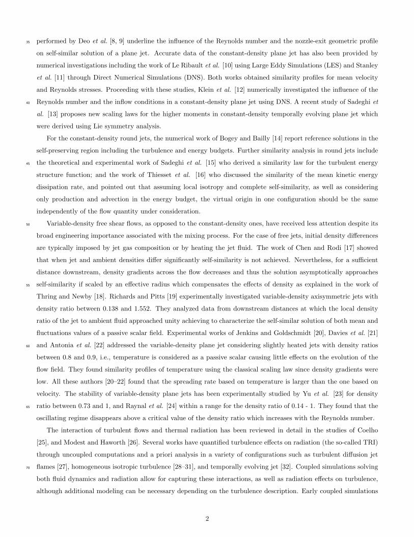
section is shown in Fig. 3a where Ue denotes the Favre average velocity excess Ue = u − U2, and ∆ Uc is180

the Favre average velocity excess at the jet centerline ∆ Uc = Uc − U2.

The inlet temperature profile that defines the heated jet is

Tin(y) =T1 + T2

2+T1 − T2

2tanh

(δ/2− |y|

2θ

). (9)

The inlet profile of the Favre average excess temperature defined as Te = T − T2 adimensionalized by the

Favre average excess temperature at the jet centerline ∆Tc = Tc − T2 is presented in Fig. 3b. Similarly, the

mean density profile at the inlet is shown in Fig. 3c.185

Synthetic turbulence generated using a Passot Pouquet model [54] is combined with the mean inlet velocity profile

at the jet region. This technique promotes turbulent instabilities and reduces the initial region of the jet. The Passot

Pouquet model defines the turbulent kinetic energy spectrum E(K) as

E(K) = A

(KKe

)4

exp

[−2

(KKe

)2], (10)

where K is the wavenumber, Ke is the wavenumber associated with the largest turbulent scales, A is an independent

variable of K defined by A = 16n3

u′2

Ke

√2/π, u′ stands for the characteristic turbulent velocity and n is the number of190

dimensions (here n = 3). Defining the auto-correlation integral scale Lc as

Lc =2βn

3Ke

√2/π with β =

2 if n = 2

π/2 if n = 3, (11)

the turbulent kinetic energy spectrum is defined by fixing the auto-correlation integral scale Lc and the turbulent

velocity u′. In the present work, these values are set to Lc = δ/2 and u′ = U1/20. Velocity fluctuations have its

maximum value at the jet centerline while are set to zero at the coflow following an hyperbolic profile analogous to

the ones of the inlet streamwise velocity and the inlet temperature. The resultant inlet averaged root-mean-square195

(rms) velocity fluctuations are shown in Fig. 3d.

Computational mesh. The grid is non-uniform in the x and y directions while it is uniform in the spanwise

direction. Computations are performed in a domain extension of 13.5δ×10δ×3δ in x, y and z directions, respectively,

while a domain extension of 10δ × 10δ × 3δ is considered to compute the statistics of the flow. The spanwise box

size is determined from an estimation of the integral length scale based on the work of Klein et al. [12]. The flow200

solution is computed using a structured grid with 566×469×149 nodes, in the x, y and z directions, respectively,

which corresponds to approximately 39.5× 106 nodes.

7

(a) (b)

(c) (d)

Figure 3: Cross-section profiles of mean (a) streamwise velocity, (b) temperature, (c) density, and (d) Reynolds stresses profiles at the

inlet boundary.

The grid spacings relevant for direct numerical simulation can be anticipated from the known behavior of turbulent

plane jets. Indeed, from scaling laws of decaying centerline profiles of temperature and velocity [20], it is possible to

estimate Tc(x) and Uc(x) for the present inlet values. Assuming constant atmospheric pressure, ρ can be estimated205

from Eq. 6, and the dynamic viscosity µ can be computed from Eq. 7. Estimating the dimensionless turbulent

kinetic energy dissipation ε∗ from previous DNS results [11], ε can be scaled for the present simulation. Then, the

grid spacing along x-axis is set to be locally maximum twice the local Kolmogorov scale η ≡(

(µ/ρ)3

ε

)1/4

. The grid

spacing along y-axis is such that the inner region of the jet (y < y1/2(x)) is as much refined as in the x direction.

Finally, the grid spacing along z-axis is uniform and equal to ∆z = δ/50, which is a close value to the ∆x and ∆y210

averages.

The Acoustic Speed Reduction method. The DNS results are here obtained by solving the compress-

ible Navier-Stokes equations through a fully-explicit formulation. Such formulation has a strong benefit for high-

performance computing since no implicit linear system needs to be solved.

When using an explicit formulation, the time step is limited by the Courant-Friedrichs-Lewy (CFL) condition215

expressed for the Courant number C

dt < Ccritmin

(∆xi|ui + c|

,∆xi|ui − c|

), (12)

8

and by the Fourier number (Fo) condition

dt < Focritmin

(∆x2

i

µ/ρ

), (13)

where ∆xi is the characteristic cell size on each i direction, c is the speed of sound, and Ccrit and Focrit are the

critical stability values for the retained numerical schemes, respectively. In the present work, the CFL condition is

more restrictive than the Fo condition. For the studied jet characterized by a low Mach number (Ma = 5.89× 10−3),220

compressible effects are negligible. In such cases, explicit numerical formulations have a notorious tendency to be

poorly efficient in terms of computational cost because of the difference between convective and sound velocities. In

this context, the so called pseudo-compressibility or artificial compressibility methods try to reduce the gap between

convective and sound velocities with artificial manipulation of the governing equations. Choi and Merkle [55] classified

the artificial compressibility methods in (1) pre-conditioning methods in which the time derivatives in the governing225

equations are multiplied by a matrix which scales the eigenvalues of the system to the same order of magnitude [55–

59], and (2) perturbation methods in which specific terms in the governing equations are manipulated in order to

replace physical acoustic waves by pseudo-acoustic modes [60–63]. The present work takes advantage of such a

perturbation method called Acoustic Speed Reduction (ASR) presented by Wang et al. [62]. The method enlarges

the allowed time step by artificially reducing the sound velocity and increasing the Mach number while keeping230

compressible effects negligible. Consequently, the computational resources needed to achieve statistical convergence

are strongly reduced. In practice, the ASR method modifies Eq. (4) by adding two new terms Sconv and Sdiff:

∂ρet∂t

+∂ (ρetui)

∂xi= −∂(puj)

∂xj+∂(τijui)

∂xj+

∂

∂xi

(λ∂T

∂xi

)+ Prad + Sconv + Sdiff, (14)

where

Sconv =

(1− 1

α2

)γp

γ − 1

∂uj∂xj

and Sdiff = −(

1− 1

α2

)[τi,j

∂ui∂xj

+∂

∂xj

(λ∂T

∂xj

)+ Prad

]. (15)

The ASR method reduces the speed of sound by an adjustable factor α accelerating the convergence of the

solution by this same factor. In the present study, the value of the factor α is set to α = 8. Such value equalizes the235

Courant-Friedrichs-Lewy and the Fourier conditions within the same order of magnitude for the current simulation.

2.2.3. Radiation simulation

A Monte Carlo Method is used in order to compute the radiative heat transfer in a participating medium. This

method consists on tracing the history of a statistically meaningful random sample of photons from their points

of emission to their points of absorption, a general description of this method applied to radiative heat transfer in240

participating medium can be found in [64]. An efficient Monte-Carlo method described in Ref. [65] is used. The

retained approach is based on an Emission-based Reciprocity Monte-Carlo method (ERM) [66] and a randomized

Quasi Monte Carlo (QMC) [67] relying on low-discrepancy Sobol sequences [68] that replace the pseudo-random

number generator to accelerate the calculation. The spectral optical properties for H2O are modelled by means of

the correlated-k (ck) narrow band model [69, 70]. The present ck model is based on updated parameters of Riviere245

and Soufiani [71].

9

The quantity of interest that is the radiative power at node i is computed from the reprocity principle as the sum

of the exchanged power P exchi,j between i and all the other cells j, i.e.,

Prad =∑j

P exchij , (16)

where P exchij is given by

P exchij =

∫ν

(κν(Ti) [Iν (Tj)− Iν (Ti)]

∫4π

Aij,νdΩ

)dν. (17)

Aij,ν accounts for all the paths between emission from the node i and absorption in any point of the cell j, after250

transmission, scattering and possible wall reflections along the paths, further details of the Monte-Carlo formulation

can be found in [66].

The Monte-Carlo method is used in this work to take advantage of its capabilities to solve the RTE with detailed

spectral radiative properties with a relatively low additional computational cost when compared with deterministic

methods such as the Discrete Ordinates Method (DOM). Also, the use of the Monte-Carlo allows for controlling the255

computation error determined as the standard deviation of the Monte-Carlo statistical estimate.

Because the computational cost of the Monte-Carlo method remains large, the grid to compute the radiative

solution fields is based on a coarser mesh than the DNS one: one out of two points is considered in each direction.

Then, the radiative solution is computed in 282 × 235 × 75 grid nodes in the x, y and z directions, respectively,

which corresponds to approximately 5×106 nodes. In order to assess the loss in accuracy embedded in considering a260

coarser mesh for the radiative solver, radiative power fields have been computed using the aforementioned DNS mesh

and the coarser mesh for a given instantaneous temperature field. Then, a comparison of the instantaneous radiative

power downstream evolution along the jet centerline for both meshes is presented in Fig. 4a, while cross-section

profiles of instantaneous radiative power at x = 10δ computed on both meshes are shown in Fig. 4b.

(a) (b)

Figure 4: Radiative power results comparison between the coarse and DNS meshes for the radiative computations. (a) Downstream

evolution of the radiative power and (b) Cross-section profiles of radiative power at x = 10δ

From the results presented in Fig. 4, it can be seen that despite some relative difference between both meshes are265

observed, the coarse mesh is able to correctly capture the trends and magnitude of the radiative power. Radiative

computations on the DNS fine mesh increases by a factor of 8 the required computational time when compared with

10

the coarse mesh. In spite of the slight degradation on accuracy, the coarser mesh is then retained in order to keep

feasible coupled DNS computations in terms of amount of CPU time and memory requirements.

Periodic boundary conditions are set in the spanwise direction: if a ray gets off the domain, for example at the270

point (x, y, Lz), it will get in at the point (x, y, 0) with the same propagation direction. All other boundaries are

treated as black-surfaces at the local temperature of the boundary node.

An additional advantage of ERM is to allow the Monte-Carlo convergence to be locally controlled. All the present

simulations are considered converged when a local error lower than 5 % of the radiative power is achieved. The error

is characterized in terms of statistical standard deviation of the estimated quantity of interest. In regions where the275

mean radiative power is close to 0 and so the relative error is difficult to converge, an absolute value of the error of

2000 W/m3 is considered to achieve convergence. This value corresponds to approximately 0.5% of the maximum

value in magnitude of the radiative power in the domain. Finally, if these two criteria are not accomplished at a

specific grid point, a maximum of 2.5× 103 rays are considered.

The radiation computation is updated every 58 iterations of the fluid flow solver. This coupling period is chosen280

keeping the coupling error below 5 % based on the Euclidean norm of the difference between the radiative power in

an iteration i, set as a reference (P irad), with respect to the radiative power after N iterations (P i+Nrad ), that is

||P i+Nrad − Pirad||2 =

√∑~xεD

(P i+Nrad (~x)− P irad(~x)

)2, (18)

where D is the computational domain. The coupling error below 5 % is chosen since the radiative solution is

considered converged when a local error lower than 5 % of the radiative power is achieved.

3. Separate validation of numerical setups in uncoupled simulations285

Results of an isothermal jet at 610 K and of the uncoupled heated jet described in §2.1 without including radiation

are first compared with experimental and numerical data available in the literature in order to validate the numerical

set up of the fluid flow solver.

In order to accelerate convergence of statistical values, all mean quantities have been averaged in the spanwise

direction. In addition, the symmetry plane about y = 0 is used to double the averaging samples.290

3.1. Results of the isothermal plane jet

The statistics are obtained by averaging the data over approximately τ = 2.4 s of physical time. This time

corresponds to approximately 11 flow time units defined as in the work of Stanley et al. [11] as τ(U1+U2)/(2Lx) = 11,

where Lx is the domain size in the x direction Lx = 10δ.

In the developed region of plane jets, the jet half-width y1/2(x) has a linear relationship with the streamwise295

coordinate [1],

y1/2

δ= K1,u

(xδ

+K2,u

), (19)

while the mean streamwise velocity excess at the jet centerline ∆Uc = uy=0 − U2 is found to vary as x−1/2,

(∆U0

∆Uc

)2

= C1,u

(xδ

+ C2,u

), (20)

11

where ∆U0 = U1−U2. The slope coefficients, K1,u and C1,u, in the fully developed region are known to be universal

in an incompressible jet; that is to say that, for large Reynolds number, they are independent of the jet conditions.

Similarly, properly scaled non-dimensional profiles become self-similar in the same region.300

Figure 5a presents the results of the growth of the jet half-width y1/2(x). Similarly, the adimensionalized mean

excess velocity decay(

∆U0

∆Uc

)2

along the jet centerline is presented in Fig. 5b. In both figures, the linear regression in

the developed region and the experimental results from the work of Thomas and Chu [72] are also shown for the sake

of comparison. Figure 5 shows that both the jet half-width and the mean velocity decay have a linear dependence

on x/δ beyond x = 8δ, which is the same value reported by Stanley et al. [11]. Hence, the coefficients for the linear305

fitting shown in Fig. 5 are computed using values in the range 8δ < x < 10δ.

(a) (b)

Figure 5: Comparison of the present isothermal plane jet results with the experimental work of Thomas and Chu [72]: downstream

evolution of (a) spread rate and (b) velocity decay. Additionally, fitted lines for y1/2 and(

∆U0∆Uc

)2are also included being K1,u = 0.088

and K2,u = 0.721; and C1,u = 0.146 and C2,u = 1.181.

The present results of the linear fitting coefficients in the self-similar zone are summarized in Table 1 along with

some experimental [7, 20, 72, 73] and DNS [11] results. The results of the virtual origins (K2,u and C2,u ) differ among

the referred works since they have a strong dependence on the inflow conditions [12, 74]. On the other hand, the

predicted slope coefficients (K1,u and C1,u ) compare generally well with previous results, although C1,u is somewhat310

lower.

Table 1: Comparison of the jet growth rate and the centerline velocity decay rate at the self-similar region between the current results

and some experimental and numerical reference values.

K1,u K2,u C1,u C2,u

Jenkins & Goldschmidt [20] 0.088 -4.5 0.160 4.0

Gutmark & Wygnanski [7] 0.100 -2.00 0.189 -4.72

Goldschmidt & Young [73] 0.0875 -8.75 0.150 -1.25

Thomas & Chu [72] 0.110 0.14 0.220 -1.19

Stanley et al. [11] 0.092 2.63 0.201 1.23

This work 0.088 0.721 0.146 1.181

Mean profiles of the excess streamwise velocity (Ue = u − U2) and the cross-stream velocity v adimen-

sionalized by ∆Uc = Uc − U2 against y/y1/2 become self-similar, that is, they collapse onto a single curve as

long as the jet is developed. Fig. 6a and 6b show that velocity profiles at x = 10δ are in good agreement with

12

self-similar profiles from experimental [7] and numerical [11] studies. The beginning of the developed zone associated315

with the self-similarity of streamwise velocity profiles is considered to begin at x = 8δ where profiles of streamwise

velocity collapse onto almost the same curve, as shown in Fig. 7. This is the same value reported by Le Ribault et

al. [10]. Likewise, the numerical study of Stanley et al. [11] obtained similar values, they found that the streamwise

velocity profiles collapse around x = 10δ. Nevertheless, experimental studies report much larger values, for example,

Gutmark and Wygnanski [7] estimate that self-similarity begins beyond x = 40δ while Bradbury [5] reports a value320

of x = 30δ. As mentioned earlier, inlet boundary conditions have a strong influence on the length of the jet potential

core. Therefore, the injection of artificial turbulence in the inlet boundary can modify the beginning of the self-

similar region. Despite the short considered domain length (10δ) in the streamwise direction which is limited; the

good agreement of velocity profiles with previous self-similar data, and the linear growth of the jet half-width and

the velocity decay indicate that the numerical domain between x = 8δ and x = 10δ is inside the developed region of325

the jet where self-similarity applies quite satisfactorily.

(a) (b)

Figure 6: Self-similar profiles of (a) streamwise and (b) cross-stream velocities of the isothermal plane jet at x = 10δ.

13

Figure 7: Cross-section profiles of streamwise velocity at several distances for the isothermal jet.

Reynolds stresses in the developed turbulent zone are also expected to become self-similar when adimensionalized

by ∆Uc and plotted against y/y1/2. Figure 8 compares the Reynolds stresses results at x = 10δ with experimental

data of Thomas and Prakash [75], Ramaprian and Chandrasekhara [76] and Bradbury [5] as well as numerical results

of Stanley at al. [11]. Predicted Reynolds stresses profiles are satisfactory although one can notice the spread of the330

reported profiles in the literature.

The general definition of turbulent kinetic energy for a variable density flow is a Favre average of the mass-

weighted fluctuations u′′i , i.e, k = 12u′′2i = 1

2 〈ρu′′2i 〉/〈ρ〉. Following the work of Chassaing et al. [77] or Huang et

al. [78], the transport equation of the turbulent kinetic energy is expressed as

1

2

∂〈ρu′′2i 〉∂t

+∂

∂xj

(1

2〈ρu′′2i 〉uj

)︸ ︷︷ ︸

Advection, 〈ρ〉 DkDt

= −〈ρu′′i u′′j 〉∂ui∂xj︸ ︷︷ ︸

Production, P

− 〈τi,j∂u′′i∂xj〉︸ ︷︷ ︸

Viscous dissipation, ε

(21)

− ∂ (〈P 〉〈u′′i 〉)∂xi

− ∂〈P ′u′′i 〉∂xi

+∂〈τi,ju′′i 〉∂xj

− ∂

∂xj〈ρu′′j

u′′2i2〉︸ ︷︷ ︸

Diffusion terms, O · T

+ 〈P ∂u′′i

∂xi〉.︸ ︷︷ ︸

Pressure-Dilatation, Π

, (22)

where the different diffusive fluxes (pressure diffusion, viscous diffusion and turbulent diffusion) have been gathered335

in the quantity denoted as T . Since velocity and Reynolds stresses profiles adimensionalized by ∆Uc are self-similar

and independent of Re in the developed region for the isothermal jet, so are the different terms in the transport

equation for turbulent kinetic energy profiles when they are adimensionalized by the scaling factor y1/2/(∆Uc3〈ρ〉).

The dimensionless transport equation of the turbulent kinetic energy is then expressed as:

Dk∗

Dt+ O · T ∗ = P∗ − ε∗ + Π∗, (23)

where ∗ denotes adimensionalized quantities. The budget of the turbulent kinetic energy in the self-similiar zone is340

presented in Fig. 9a, while Figs. 9b to 9e show the results of each term in the turbulent kinetic energy equation

compared with experimental data of Terashima et al. [79] and numerical results of Stanley et al. [11]. The profiles

are obtained by averaging the scaled simulation fields in the range 9δ < x < 10δ. The pressure-dilatation term (Π∗)

14

(a) (b)

(c) (d)

Figure 8: Self-similar Reynolds stresses profiles of the isothermal plane jet in the (a) x direction, (b) z direction, (c) y direction; and (d)

shear stress at x = 10δ.

has a negligible contribution; in consequence, it is not included in Fig. 9. All trends in the budget are well captured

and compare reasonably good with experimental results, even improving the results from past numerical simulations.345

The two main terms in the energy budget are production and dissipation. Viscous dissipation is almost constant

in the core of the jet (y < y1/2) while production has a strong peak around y = 0.8y1/2 in agreement with the

Reynolds stresses presented in Fig. 8. The turbulent kinetic energy generated at the peak of production is advected

to the jet centerline through entrainment velocity while turbulent diffusion spread the turbulent kinetic energy to

both the jet centerline and the jet edge. At the center of the jet, turbulent fluctuations are maintained solely through350

advection and turbulent diffusion. The low value of the unbalance among all terms (—Unbalance, in Fig. 9a) points

out that the simulation is capturing all the physical mechanism in which turbulence is produced, dissipated and

transported.

Figure 10 presents the one-dimensional autospectrum along the homogeneous spanwise direction of the streamwise

velocity fluctuations, Eu(K), at x = 10δ in the jet centerline, which is adimensionalized by the streamwise velocity355

fluctuations u′′u′′ at the jet centerline and the jet half width y1/2. The one-dimensional autospectrum is plotted

against two different horizontal axis: at the bottom one, wavenumbers are scaled by the length of large turbulent

motions; while in the top horizontal axis, wavenumbers are scaled by the characteristic length of the smallest eddies

η ≡(

(µ/ρ)3

ε

)1/4

. Moreover, the one-dimensional autospectrum from Stanley et al. [11] is also plotted for the sake

15

(a)

(b) (c)

(d) (e)

Figure 9: (a) Budget of dimensionless turbulent kinetic energy of the isothermal plane in the developed region. Components of the

turbulent kinetic energy budget: (b) production, (c) turbulent diffusion, (d) advection and (e) dissipation compared with experimental

data of Terashima et al. [79] and numerical results of Stanley et al. [11].

of comparison. Stanley et al. [11] reported results of the autospectrum in time of the streamwise velocity on the360

centreline of the jet at x = 10δ, their results are here plotted in terms of the wavenumber by invoking the Taylor

hypothesis. Applying here such an hypothesis results in a spatial spectrum along the streamwise direction, which is

homogeneous in the developed region when appropriately scaled, but not isotropic. Then, a disagreement is found in

the large scale motions due to its high correlation along the streamwise direction. However, the present results are in

very good agreement with [11] at higher wavenumbers (say (K/2π)y1/2 > 4) since all fluctuations are isotropic in this365

region. Furthermore, the present DNS simulation even improves the resolution at the dissipative region comparing

with the spectrum in [11]. When looking at the top horizontal axis in Fig. 10, the dive of the profile occurs at a

location close to the expected wavenumber when compared to reference dissipative spectra presented, for example,

in [4]. The presented spectra together with the low value of the unbalance term in Fig. 9a demonstrate that the

dissipation can be attributed to the physical viscous dissipation, rather than to the numerical dissipation introduced370

by the retained discretization scheme or filtering.

3.2. Results of the uncoupled heated plane jet

Mean results of the uncoupled heated jet are computed by averaging the data over approximately τ = 2.4 s of

physical time, which is equivalent to 11 flow time units. In the case of the uncoupled studied heated jet described in

§2.1, one is interested in the turbulent mixing of the temperature field. Additionally, the associated variable density375

field can modify the turbulent transfer of momentum and make the temperature mixing deviate from the behavior

of a passive scalar in a turbulent jet. In this subsection, the solution of the heated jet is compared with reported

experimental data of the slightly heated plane jet and numerical data of the evolution of a passive scalar field in a

plane jet.

16

Figure 10: One-dimensional autospectra along the homogeneous spanwise direction of the centerline longitudinal velocity fluctuations at

x = 10δ adimensionalized by the streamwise velocity fluctuations u′′u′′ at the jet centerline and the jet half width y1/2 for the present

work (dashed black line). Results from Stanley et al. [11] (solid blue line). Bottom horizontal axis: wavenumbers scaled by the length of

large turbulent motions. Top horizontal axis: wavenumbers scaled by the characteristic length of the smallest eddies.

Figure 11 describes key features of the downstream evolution of mean temperature and compares them with380

numerical results of Stanley et al. [11] who analyzed the evolution of a passive scalar field using a unity Schmidt

number, and with experimental results of a heated plane jet of Browne et al. [80] who set an initial excess temperature

of ∆T0 = T1 − T2 = 25 K. Similar to the jet half-width based on the mean streamwise velocity y1/2, the half-width

based on temperature y1/2,T is the distance from the center of the jet where the corrected temperature Te = T−T2

is half the corrected temperature at the jet center ∆Tc = Ty=0 − T2. In Figure 11a, results of the evolution of385

the half-width of the jet based on temperature are compared with the numerical results of Stanley et al. [11] and the

experimental data of Browne et al. [80]. The results of the current heated jet show a slow initial developing when

compared with the data of Browne et al. [80] and Stanley et al. [11] in which the half-width linear growth appears

beyond x = 4δ and x = 6δ, respectively; while for the present results linear growth is shown beyond x = 7δ. As for

the results of the velocity fields in the isothermal plane jet, the strong dependence of the initial developing zone on390

the inflow conditions explains the scatter among the different works, while the slope of the downstream evolution of

y1/2,T compares well with previous works. Figure 11b shows the temperature decay in the jet centerline in which

∆T0 = T1 − T2 and ∆Tc = Ty=0 − T2. The results of the temperature decay are in good agreement with the

mean scalar decay of Stanley et al. [11]. Results of the temperature decay of Browne et al. [80] have a faster initial

developing, probably due to the inflow conditions, while the decay rate is greater than the decay predicted by both395

the current numerical results and the simulation of Stanley et al. [11].

In Figure 12a, the Favre averaged temperature corrected by the coflow temperature Te = T−T2 adimension-

17

(a) (b)

Figure 11: Downstream evolution of mean temperature field: (a) jet spread based on temperature and (b) temperature decay along the

jet centerline.

alized by ∆Tc = Ty=0 − T2 is plotted against y/y1/2,T at x = 10δ and compared with experimental results from

Davies et al. [21] who set an initial excess temperature of ∆T0 = 14.6 K, the study of Jenkins and Goldschmidt [20]

that fixed this value to ∆T0 = 20.7 K, and the experimental results of Antonia et al. [22] with an excess temperature400

at the inlet section of ∆T0 = 25 K; while the excess temperature in the current simulation is ∆T0 = T1−T2 = 480 K.

Despite the ∆T0 disparity among the present work and the values found in the literature, the dimensionless tem-

perature profile is in good agreement with experimental results. Additionally, Figure 12b compares the downstream

evolution of the temperature fluctuations along the jet centerline with experimental results of Browne et al. [80] and

the growth of the centerline scalar fluctuations of Stanley et al. [11]. Results from Browne et al. [80] have a faster405

initial developing and higher fluctuations intensity, this may explain the results of the temperature decay presented

in Fig. 11b. The current results of temperature fluctuations have the same tendency as previous data, which is a

strong growth of the fluctuations at the end of the initial developing zone followed by a slow decay downstream.

(a) (b)

Figure 12: (a) Dimensionless Favre averaged temperature profiles of the heated plane jet without including radiation at x = 10δ compared

with experimental results of Davies et al. [21], Jenkins and Goldschmidt [20], and Antonia et al. [22]. (b) Downstream evolution of

temperature fluctuations at the jet centerline compared with experimental data of Browne et al. [80] and numerical results of Stanley et

al. [11].

Integrating the x-momentum boundary-layer equation with respect to y, the momentum flow rate per unit span,

defined as∫ +∞−∞ 〈ρu

2〉dy, is constant along the streamwise direction of the plane jet. Due to the presence of a coflow410

18

stream, this quantity is infinite and is here replaced by

Mx =

∫ +∞

−∞

(〈ρu2〉 − ρ2U

22

)dy, (24)

Results of the momentum flow rate adimensionalized by its value at the initial cross-section are presented in

Fig. 13 for both the isothermal and the heated jets. Additionally, an horizontal dashed line corresponding to the

ideal behaviour of the jet is included in Fig. 13. As expected, the momentum flow rate is almost constant along the

streamwise direction for both cases, i.e., Mx deviations from the ideal plane jet are less than 1.3%.415

Figure 13: Evolution of momentum flow rate per unit span along x direction.

As detailed in the work of Foysi et al. [81], the conservation of momentum flux in the developed region yields that

the ratio between 〈ρc〉∆Uc2y1/2 and ρ0∆U20 δ is constant, where 〈ρc〉 is the mean density at the jet centerline and

ρ0 is the jet density at the exit nozzle. An equivalent jet opening rε = δ (ρ0/〈ρc〉) is defined, where the exit nozzle

density is considered as the bulk average ρ0 = 1δ

∫δρ|x=0

dy. As reported in the work of Richards and Pitts [19], rε

can be interpreted physically as the width opening of a hypothetical jet of density 〈ρc〉 with the same initial mass420

and momentum fluxes as the jet under consideration. Then, the conservation of momentum flux can be written as

∆Uc2y1/2

∆U20 rε

∼ constant, (25)

As shown in Fig. 14, the velocity decays of the heated and isothermal jets almost collapse on the same curve when

(∆U0/Uc)2is plotted against x/rε (Fig. 14b), while these curves have a clearly different slope when plotted against

x/δ (Fig. 14a). Note, that the scaled velocity decay of the heated jet in Fig. 14b has values beyond x = 10rε since

rε < δ.425

(a) (b)

Figure 14: Centerline velocity decay against (a) x/δ and (b) x/rε.

19

4. Results of the heated plane jet coupled with radiative energy transfer

In this section, the effects of radiation on mean quantities and its fluctuations are analyzed by comparing the

heated jet without radiation (NR) and including radiation (R). The statistics are obtained by averaging the data

over approximately τ = 1 s of physical time. This time corresponds to approximately 4.6 flow time units defined

as τ(U1 + U2)/(2Lx) = 4.6, where Lx is the domain size in the x direction Lx = 10δ. For the same amount of430

physical time, the computational resources to compute the coupled jet are approximately 3.5 times greater than the

uncoupled simulation.

4.1. Velocity field

Radiation effects on velocity are indirectly caused by changes in density due to the modified temperature field.

As shown in Fig. 15a, the inclusion of radiation has a negligible effect on the scaled mean velocity profiles at x = 10δ.435

Moreover, the downstream centerline velocity decay presented in Fig. 15b shows that, when scaled by rε, radiation

does not modify the velocity decay since the slightly changes in density are compensated by rε.

(a) (b)

Figure 15: Comparisons between the radiative (R) and the non-radiative (NR) cases of (a) the cross-section streamwise velocity profiles

at x = 10δ and (b) the downstream velocity decay along the jet centerline scaled by rε.

Reynolds stresses are slightly modified by thermal radiation. Figure 16 shows cross-sections profiles of normal

and shear Reynolds stresses at x = 10δ for the radiative and non-radiative cases.

(a) (b) (c) (d)

Figure 16: Comparisons of the dimensionless Reynolds stresses profiles at x = 10δ in the (a) streamwise, (b) cross-stream and (c) spanwise

directions, and (d) Reynolds shear stress profiles between the radiative (R) and the non-radiative (NR) cases.

In accordance with previous coupled DNS studies [37, 46–48], weak radiation effects on first and second moment440

orders of velocity are observed in non-reactive flows. Radiation effects on velocity are indirectly caused by changes

in density, while effects on temperature are directly caused by the radiative power field.

20

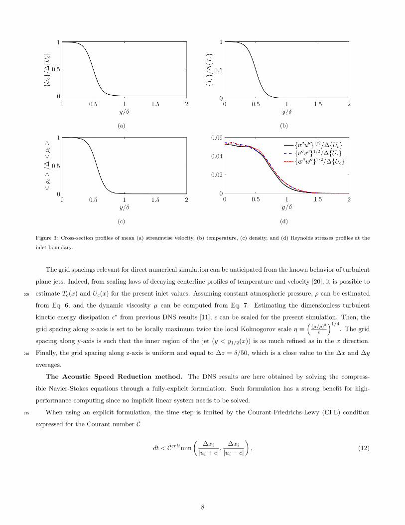
4.2. Radiative power field

A slice of the instantaneous radiative power at z = 0 is presented in Fig. 17a, while Fig. 17b shows the averaged

radiative power 〈Prad〉. Radiative power is a balance between the power lost by emission and the power gained due445

to absorption, thus regions with negative values of Prad are cooling down by the effect of radiation, while regions

with positive values are heating up due to radiation. As expected, Fig. 17 shows that the centerline of the jet, which

is the hottest region of the flow, loses heat by radiation. On the other hand, thermal radiation energy is further

absorbed at colder regions of the jet, tending to a null radiative power as the distance to the jet centerline increases.

In Fig. 17b, in which radiative power averaged over time is shown, the emission dominated region has been delimited450

from the absorption dominated region by a solid black line corresponding to the isoline of Prad = 0.

(a) (b)

Figure 17: (a) Instantaneous radiative power field at z = 0. (b) Mean exchanged radiative power field, a solid black line delimits the

emission dominated region from the absorption dominated region.

.

The initial zone in which the jet develops is the most affected region by radiation due to the large temperature

gradients. Then, radiative power at the jet centerline tends to zero downstream. Regarding a cross-section profile of

the jet, a large radiative power is emitted in the centerline, then radiative power tends to zero in the jet edge while

an absorption dominated zone is developed at the outer region of the jet. In the developed region the temperature455

and its gradients are lower and the heat transport by radiation decreases significantly.

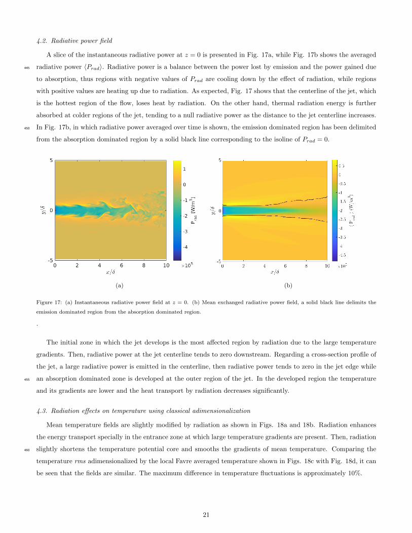
4.3. Radiation effects on temperature using classical adimensionalization

Mean temperature fields are slightly modified by radiation as shown in Figs. 18a and 18b. Radiation enhances

the energy transport specially in the entrance zone at which large temperature gradients are present. Then, radiation

slightly shortens the temperature potential core and smooths the gradients of mean temperature. Comparing the460

temperature rms adimensionalized by the local Favre averaged temperature shown in Figs. 18c with Fig. 18d, it can

be seen that the fields are similar. The maximum difference in temperature fluctuations is approximately 10%.

21

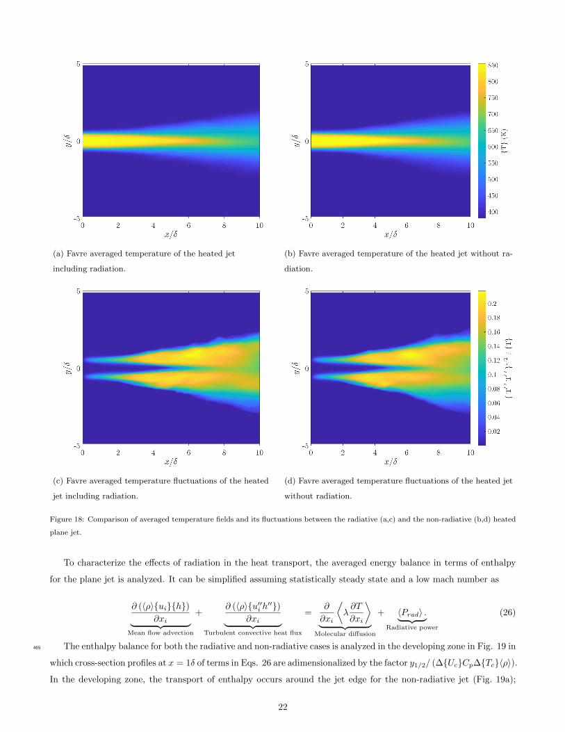
(a) Favre averaged temperature of the heated jet

including radiation.

(b) Favre averaged temperature of the heated jet without ra-

diation.

(c) Favre averaged temperature fluctuations of the heated

jet including radiation.

(d) Favre averaged temperature fluctuations of the heated jet

without radiation.

Figure 18: Comparison of averaged temperature fields and its fluctuations between the radiative (a,c) and the non-radiative (b,d) heated

plane jet.

To characterize the effects of radiation in the heat transport, the averaged energy balance in terms of enthalpy

for the plane jet is analyzed. It can be simplified assuming statistically steady state and a low mach number as

∂ (〈ρ〉uih)∂xi︸ ︷︷ ︸

Mean flow advection

+∂ (〈ρ〉u′′i h′′)

∂xi︸ ︷︷ ︸Turbulent convective heat flux

=∂

∂xi

⟨λ∂T

∂xi

⟩︸ ︷︷ ︸

Molecular diffusion

+ 〈Prad〉 .︸ ︷︷ ︸Radiative power

(26)

The enthalpy balance for both the radiative and non-radiative cases is analyzed in the developing zone in Fig. 19 in465

which cross-section profiles at x = 1δ of terms in Eqs. 26 are adimensionalized by the factor y1/2/ (∆UcCp∆Tc〈ρ〉).

In the developing zone, the transport of enthalpy occurs around the jet edge for the non-radiative jet (Fig. 19a);

22

while in the radiative jet, showed in Fig. 19b, a significant enthalpy transport occurs in the jet core due to radiation

and it is compensated by mean flow advection. Mean flow advection and turbulent convective heat flux have opposite

effects. However, because turbulence has not yet penetrated in the jet centerline in the developing zone, turbulent470

convective heat flux has null effects in the jet core.

(a) (b)

Figure 19: Cross-section profiles of the enthalpy budget main terms at x = δ for (a) the non-radiative and (b) the radiative jets.

Figure 20 shows an analysis of the enthalpy balances in the developed region (x=10δ). Again, all terms of the

balances have been adimensionalized by the factor y1/2/ (∆UcCp∆Tc〈ρ〉). It can be seen that the mean flow

advection and the turbulent convective heat flux term strongly dominate the enthalpy balance in the studied case.

The radiation term in the balance of Eq. 26 has a negligible contribution at the developed zone but it is significant475

in the developing zone. This situation is produced due to the lower temperature gradients involved in the developed

zone and the increased turbulent fluctuations in the developed zone which enhance the turbulent convective heat flux.

(a) (b)

Figure 20: Cross-section profiles of the enthalpy budget main terms at x = 10δ for (a) the non-radiative and (b) the radiative jets.

Mean temperature decay which provides a measure of the overall cooling of the jet is shown in Fig. 21a where

∆T0 = T1−T2 and ∆Tc = Ty=0−T2. Surprisingly, despite the fact that radiation has no effects on the developed

zone, as shown in Fig. 20, the mean temperature at the jet centerline decays faster in the radiative case than in the480

non-radiative case. In Figure 20 fitted lines are added in the region 8 < x/δ < 10. Figure 21b shows that the jet

half-with based on temperature for the radiative case is slightly larger than for the non-radiative case. Temperature

profiles of the uncoupled and coupled heated jets, shown in Fig. 21c, collapse almost in the same curve when the y

coordinate is adimensionalized by y1/2,T .

23

(a) Downstream temperature decay along the jet centerline. (b) Downstream jet spread based on temperature.

(c) Cross-section profile of mean excess temperature adimen-

sionalized by the mean excess centerline temperature at x =

10δ .

Figure 21: Comparison of mean temperature-related quantities between the radiative (R) and the non-radiative (NR) jets. Fitted

lines(

∆T0∆Tc

)2= Q1,T

(xδ

+Q2,T

)are defined by Q1,T = 0.3697 and Q2,T = −2.9090 for the NR case; and Q1,T = 0.4517 and

Q2,T = −3.2460 for the R case.

Figure 22a shows the root-mean-square of temperature fluctuations along the jet centerline adimensionalized485

by the local Favre average excess temperature. While for the non-radiative jet, temperature fluctuations start to

develop beyond x = 4δ, in the radiative case, temperature fluctuations start further downstream and its intensity

remains slightly lower than in the non-radiative jet. Dimensionless cross-section profiles of temperature fluctuations

at x = 10δ are presented in Fig. 22b. Temperature fluctuations almost collapse onto the same curves with classical

adimensionalization although slightly different trends can be observed.490

(a) Downstream evolution of dimensionless temperature fluc-

tuations along the jet centerline.(b) Cross-section profile of dimensionless temperature fluctu-

ations at x = 10δ.

Figure 22: Comparison of temperature fluctuations-related quantities between the radiative and the non-radiative plane jet.

24

4.4. A novel adimensionalization for the mean temperature field to correct variable density effects

As observed in Fig. 21a, the classical adimensionalization fails to give the same slope for the temperature decay

between radiative and non-radiative cases despite the negligible contribution of radiation in the developed region.

In this section, a novel adimensionalization based on approximate conservation of the convective heat flux is derived

in order to collapse the temperature decay of different heated jets even though developing conditions are different.495

This assumption is exact for negligible coflow and radiative effects. It allows here to correct variable density effects

for the investigated case with moderate radiative transfer. This adimensionalization can then be used to distinguish

whether radiation changes the dynamic mechanisms in the developed region or not.

Conservation of the convective heat flux in a free jet can be expressed by the equation

∂

∂x

∫ +∞

−∞〈ρ〉u∆Tedy = 0, (27)

For the new scaling, temperature and density fields are assumed self-similar in the form ∆Te = ∆TcfT (η)500

and 〈ρ〉 = 〈ρc〉fρ(η). Considering a strong jet with minor co-flow effects, velocity self-similarity is expressed in the

form u = Ucfu(η). Note that ∆Tc, 〈ρc〉 and Uc are respectively temperature, density and velocity scales

that depend only on downstream position, while fT (η), fρ(η) and fu(η) are distribution functions depending on the

dimensionless coordinate η = y/y1/2,T . The choice of a unique length scale, in this case y1/2,T , implies that self-

similarity on temperature, density and velocity can be described with the same local length scale, which is consistent505

since the jet growths are proportional among them. Then, Eq. 27 can be written as

〈ρc〉Uc∆Tcy1/2,T

∫ +∞

−∞fT (η)fρ(η)fu(η)dη = constant, (28)

which implies that the product 〈ρc〉Uc∆Tcy1/2,T is independent of x in the self-similar region. Then, in this

region, the convective heat flux conservation can be expressed as

〈ρc〉Uc∆Tcy1/2,T

ρ0 u0∆T0δ= constant. (29)

where u0 = 1δ

∫δUin(y)dy is analogous to ρ0 defined in §3.2

Similar to the derivation of the scaling for the velocity decay in the jet centerline [81], it is possible to deduce a510

scaling for the temperature decay. Defining an equivalent heat jet opening characterizing thermal transfer, rε,T , as

rε,T =δ2

y1/2,T

(ρ0

〈ρc〉

)2(u0

Uc

)2

, (30)

the convective heat flux conservation presented in Eq. (29) can be expressed as

(∆Tc∆T0

)2 y1/2,T

rε,T= constant. (31)

Then, similar to Eqs. (19) and (20), the temperature decay (∆T0/∆Tc)2in the self-similar region has a linear

relationship with the streamwise coordinate in the form

(∆T0

∆Tc

)2

= Q1,T

(x

rε,T+Q2,T

), (32)

25

assuming self-preserving temperature, density and velocity distributions; the temperature decay of heated jets has a515

universal behavior in the self-similar region when adimensionalized by the equivalent heat jet opening introduced in

Eq. (30).

4.5. Radiation effects on temperature using the new scaling

Figure 23 shows again the centerline temperature decay and temperature profiles of the uncoupled and coupled jets

but this time using the equivalent heat jet opening based on the convective heat flux conservation to scale the results.520

Additionally, the linear regressions of the centerline temperature decay in the developed region (8δ < x < 10δ) is

shown in Fig. 23a. In contrast with Fig. 21a, it can be observed that in Fig. 23a the temperature decays of the

radiative and the non-radiative jets collapse into almost the same curve presenting nearly the same slope when the x-

coordinate is scaled by rε,T . Figure 23b shows the collapse of temperature profiles for the radiative and non-radiative

jets at the same x = 9rε,T which actually corresponds to x = 9.76δ for the non-radiative jet and to x = 9.15δ for the525

radiative jet, although the classical scaling was already collapsing mean temperature profiles onto almost the same

curve.

(a) Scaled downstream temperature decay along the jet cen-

terline.

(b) Cross-section profile of mean excess temperature adi-

mensionalized by the mean excess centerline temperature at

x = 9rε,T .

Figure 23: Comparison of mean temperature-related quantities between the radiative (R) and the non-radiative (NR) jets scaled using

rε,T . Fitted lines(

∆T0∆Tc

)2= Q1,T

(x

rε,T+Q2,T

)are defined by Q1,T = 0.2505 and Q2,T = 1.0962 for the NR case; and Q1,T = 0.2513

and Q2,T = 1.6099 for the R case.

In order to quantitatively compare the behavior of the temperature decay between the radiative and non-radiative

jets, results of the linear fitting coefficients in the self-similar zone (beyond x = 7δ) for both the new scaling (using

rε,T in Eq. 32) and the classical scaling (using δ instead of rε,T in Eq. 32) are summarized in Table 2.530

On the one hand, values of Q2,T differ between R and NR cases for both scalings due to the inclusion of the

radiative heat exchange which affects the developing zone. On the other hand, while Q1,T coefficients are significantly

different (22.2%) when comparing R and NR cases using the classical scaling, they have a small difference (0.32 %)

using the new scaling based on the equivalent heat jet opening.

Temperature fluctuations along the jet centerline for the radiative and non-radiative jets are shown in Fig. 24a535

adimensionalized using rε,T . The intensity of the temperature fluctuations is first slightly lower for the radiative case

at the developing region in which radiation has a significant impact on the flow. However, once in the developed region,

the intensity of temperature fluctuations at the jet centerline collapses almost into the same value. Additionally,

26

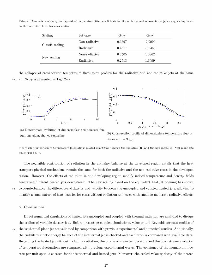
Table 2: Comparison of decay and spread of temperature fitted coefficients for the radiative and non-radiative jets using scaling based

on the convective heat flux conservation.

Scaling Jet case Q1,T Q2,T

Classic scalingNon-radiative 0.3697 -2.9090

Radiative 0.4517 -3.2460

New scalingNon-radiative 0.2505 1.0962

Radiative 0.2513 1.6099

the collapse of cross-section temperature fluctuation profiles for the radiative and non-radiative jets at the same

x = 9rε,T is presented in Fig. 24b.540

(a) Downstream evolution of dimensionless temperature fluc-

tuations along the jet centerline.(b) Cross-section profile of dimensionless temperature fluctu-

ations at x = 9rε,T .

Figure 24: Comparison of temperature fluctuations-related quantities between the radiative (R) and the non-radiative (NR) plane jets

scaled using rε,T .

The negligible contribution of radiation in the enthalpy balance at the developed region entails that the heat

transport physical mechanisms remain the same for both the radiative and the non-radiative cases in the developed

region. However, the effects of radiation in the developing region modify indeed temperature and density fields

generating different heated jets downstream. The new scaling based on the equivalent heat jet opening has shown

to counterbalance the differences of density and velocity between the uncoupled and coupled heated jets, allowing to545

identify a same nature of heat transfer for cases without radiation and cases with small-to-moderate radiative effects.

5. Conclusions

Direct numerical simulations of heated jets uncoupled and coupled with thermal radiation are analyzed to discuss

the scaling of variable density jets. Before presenting coupled simulations, velocity and Reynolds stresses profiles of

the isothermal plane jet are validated by comparison with previous experimental and numerical studies. Additionally,550

the turbulent kinetic energy balance of the isothermal jet is checked and each term is compared with available data.

Regarding the heated jet without including radiation, the profile of mean temperature and the downstream evolution

of temperature fluctuations are compared with previous experimental works. The constancy of the momentum flow

rate per unit span is checked for the isothermal and heated jets. Moreover, the scaled velocity decay of the heated

27

and isothermal jets collapses almost onto the same curve. These uncoupled results demonstrate the adequacy of the555

DNS numerical setup. The inlet velocity profile is here combined with artificial turbulence to shorten the domain

with a quick destabilization of the potential core to yield a reduced computational time. Despite the limited extent of

the present domain; the obtained profiles of first and second order moments of velocity fields beyond x = 8δ compare

quite well with previous self-similar profiles, and besides, linearity in the velocity decay rate and the jet half-width

growth is observed in the region 8δ ≤ x ≤ 10δ.560

In the coupled case with radiation, an analysis of the enthalpy balance at the initial zone shows that radiation

has a major contribution of heat transport modifying temperature and density fields. On the other hand, a negligible

radiative contribution is found in the developed region. Thus, for both uncoupled and coupled heated jets, the

nature of heat transfer remain the same, which is here the turbulent heat transport. However, despite this minor

contribution of radiation in the developed region, the classical jet scaling law fails to give the same temperature565

decay slope between the radiative and non-radiative cases. This could wrongly lead to conclude on a modified

balance of heat transport mechanisms in the studied case. In fact, thermal radiation can have two kind of effects

on the temperature profile: a direct one from radiative energy transfer and an indirect one due to the modified flow

density.

The proposed equivalent heat jet opening deduced from the convective heat flux conservation equation has shown570

to compensate density differences to collapse both radiative and non-radiative jets profiles onto the same temperature

decay rate in the developed region. This scaling accounts for the indirect effects of variable density in cases with

radiation. It allows for distinguishing whether radiation modifies the heat transfer mechanisms in the developed

region or not. In the studied case, it is now clearly identified that is does not.

The present results achieved with DNS coupled to a ck model and Monte-Carlo to describe radiation may serve575

as a reference case to compare simplified approaches such as LES for the turbulence model, or Weighted Sum of Gray

Gases (WSGG) and its modern variants for modeling radiative properties combined with deterministic approaches

to solve the RTE like DOM.

Further investigations with larger impact of radiation will be carried out in the future and will benefit from the

derived scaling law to discriminate strong radiative impact from indirect effects on the modification of the density580

field.

Acknowledgments

The authors wish to thank CAPES (Brazilian Federal Agency for Support and Evaluation of Graduate Education

within the Ministry of Education of Brazil) and Centrale Recherche S.A. for the financial support. This work

was performed using HPC resources from the Mesocentre computing center of CentraleSupelec and Ecole Normale585

Superieure Paris-Saclay supported by CNRS and Region Ile-de-France (http://mesocentre.centralesupelec.fr/). It

was also granted access to the HPC resources of CINES under the allocation 2018-A0042B10159 made by GENCI.

References

[1] N. Rajaratnam, Turbulent jets., Elsevier Scientific, New York, 1976.

[2] A. A. Townsend, The structure of turbulent shear flow, Cambridge university press, 1980.590

28

[3] G. N. Abramovich, The theory of turbulent jets, M.I.T. Press, 1963.

[4] S. B. Pope, Turbulent flows, IOP Publishing, 2001.

[5] L. Bradbury, The structure of a self-preserving turbulent plane jet, Journal of Fluid Mechanics 23 (01) (1965) 31–64.

[6] G. Heskestad, Hot-wire measurements in a plane turbulent jet, Journal of Applied Mechanics 32 (4) (1965) 721–734.

[7] E. Gutmark, I. Wygnanski, The planar turbulent jet, Journal of Fluid Mechanics 73 (03) (1976) 465–495.595

[8] R. C. Deo, J. Mi, G. J. Nathan, The influence of reynolds number on a plane jet, Physics of Fluids 20 (7) (2008) 075108.

[9] R. C. Deo, J. Mi, G. J. Nathan, The influence of nozzle-exit geometric profile on statistical properties of a turbulent plane jet,

Experimental Thermal and Fluid Science 32 (2) (2007) 545–559.

[10] C. Le Ribault, S. Sarkar, S. Stanley, Large eddy simulation of a plane jet, Physics of Fluids 11 (10) (1999) 3069–3083.

[11] S. Stanley, S. Sarkar, J. Mellado, A study of the flow-field evolution and mixing in a planar turbulent jet using direct numerical600

simulation, Journal of Fluid Mechanics 450 (2002) 377–407.

[12] M. Klein, A. Sadiki, J. Janicka, Investigation of the influence of the reynolds number on a plane jet using direct numerical simulation,

International Journal of Heat and Fluid Flow 24 (6) (2003) 785–794.

[13] H. Sadeghi, M. Oberlack, M. Gauding, On new scaling laws in a temporally evolving turbulent plane jet using lie symmetry analysis

and direct numerical simulation, Journal of Fluid Mechanics 854 (2018) 233–260.605

[14] C. Bogey, C. Bailly, Turbulence and energy budget in a self-preserving round jet: direct evaluation using large eddy simulation,

Journal of Fluid Mechanics 627 (2009) 129–160.

[15] H. Sadeghi, P. Lavoie, A. Pollard, Equilibrium similarity solution of the turbulent transport equation along the centreline of a round

jet, Journal of Fluid Mechanics 772 (2015) 740–755.

[16] F. Thiesset, R. Antonia, L. Djenidi, Consequences of self-preservation on the axis of a turbulent round jet, Journal of Fluid Mechanics610

748.

[17] C. J. Chen, W. Rodi, Vertical turbulent buoyant jets: a review of experimental data, Nasa STI/Recon Technical Report A 80 (1980)

–.

[18] M. Thring, M. Newby, Combustion length of enclosed turbulent jet flames, Symposium (International) on Combustion (1953)

789–796.615

[19] C. D. Richards, W. M. Pitts, Global density effects on the self-preservation behaviour of turbulent free jets, Journal of Fluid

Mechanics 254 (1993) 417–435.

[20] P. Jenkins, V. Goldschmidt, Mean temperature and velocity in a plane turbulent jet, Journal of Fluids Engineering 95 (4) (1973)

581–584.

[21] A. Davies, J. Keffer, W. Baines, Spread of a heated plane turbulent jet, The physics of fluids 18 (7) (1975) 770–775.620

[22] R. Antonia, L. Browne, A. Chambers, S. Rajagopalan, Budget of the temperature variance in a turbulent plane jet, International

Journal of Heat and Mass Transfer 26 (1) (1983) 41–48.

[23] M.-H. Yu, P. A. Monkewitz, Oscillations in the near field of a heated two-dimensional jet, Journal of fluid mechanics 255 (1993)

323–347.

[24] L. Raynal, J.-L. Harion, M. Favre-Marinet, G. Binder, The oscillatory instability of plane variable-density jets, Physics of Fluids625

8 (4) (1996) 993–1006.

[25] P. J. Coelho, Numerical simulation of the interaction between turbulence and radiation in reactive flows, Progress in Energy and

Combustion Science 33 (4) (2007) 311–383.

[26] M. F. Modest, D. C. Haworth, Radiative Heat Transfer in Turbulent Combustion Systems: Theory and Applications, Springer, 2016.

[27] P. Coelho, Detailed numerical simulation of radiative transfer in a nonluminous turbulent jet diffusion flame, Combustion and flame630

136 (4) (2004) 481–492.

[28] F. Kritzstein, A. Soufiani, Infrared gas radiation from a homogeneously turbulent medium, International journal of heat and mass

transfer 36 (7) (1993) 1749–1762.

[29] C. B. da Silva, I. Malico, P. J. Coelho, Radiation statistics in homogeneous isotropic turbulence, New Journal of Physics 11 (9)

(2009) 093001.635

[30] M. Roger, C. B. Da Silva, P. J. Coelho, Analysis of the turbulence–radiation interactions for large eddy simulations of turbulent

flows, International Journal of Heat and Mass Transfer 52 (9-10) (2009) 2243–2254.

[31] M. Roger, P. J. Coelho, C. B. da Silva, The influence of the non-resolved scales of thermal radiation in large eddy simulation of

29

turbulent flows: A fundamental study, International Journal of Heat and Mass Transfer 53 (13-14) (2010) 2897–2907.

[32] M. Roger, P. Coelho, C. Da Silva, Relevance of the subgrid-scales for large eddy simulations of turbulence–radiation interactions in640

a turbulent plane jet, Journal of Quantitative Spectroscopy and Radiative Transfer 112 (7) (2011) 1250–1256.

[33] L. Tesse, F. Dupoirieux, J. Taine, Monte carlo modeling of radiative transfer in a turbulent sooty flame, International journal of

heat and mass transfer 47 (3) (2004) 555–572.

[34] G. Li, M. F. Modest, Importance of turbulence-radiation interactions in turbulent diffusion jet flames, Journal of heat transfer

125 (5) (2003) 831–838.645

[35] T. Ren, M. F. Modest, S. Roy, Monte carlo simulation for radiative transfer in a high-pressure industrial gas turbine combustion

chamber, Journal of Engineering for Gas Turbines and Power 140 (5) (2018) 051503.

[36] A. Gupta, D. Haworth, M. Modest, Turbulence-radiation interactions in large-eddy simulations of luminous and nonluminous

nonpremixed flames, Proceedings of the Combustion Institute 34 (1) (2013) 1281–1288.

[37] S. Ghosh, R. Friedrich, M. Pfitzner, C. Stemmer, B. Cuenot, M. El Hafi, Effects of radiative heat transfer on the structure of650

turbulent supersonic channel flow, Journal of Fluid Mechanics 677 (2011) 417–444.

[38] D. Poitou, J. Amaya, M. El Hafi, B. Cuenot, Analysis of the interaction between turbulent combustion and thermal radiation using

unsteady coupled LES/DOM simulations, Combustion and Flame 159 (4) (2012) 1605–1618.

[39] W. Jones, M. Paul, Combination of DOM with LES in a gas turbine combustor, International journal of engineering science 43 (5-6)

(2005) 379–397.655

[40] S. Berger, S. Richard, F. Duchaine, G. Staffelbach, L. Gicquel, On the sensitivity of a helicopter combustor wall temperature to

convective and radiative thermal loads, Applied Thermal Engineering 103 (2016) 1450–1459.

[41] C. Koren, R. Vicquelin, O. Gicquel, Multiphysics simulation combining large-eddy simulation, wall heat conduction and radiative

energy transfer to predict wall temperature induced by a confined premixed swirling flame, Flow, Turbulence and Combustion 101 (1)

(2018) 77–102.660

[42] Y. Wu, D. Haworth, M. Modest, B. Cuenot, Direct numerical simulation of turbulence/radiation interaction in premixed combustion

systems, Proceedings of the Combustion Institute 30 (1) (2005) 639–646.

[43] Y. Wu, M. F. Modest, D. C. Haworth, A high-order photon monte carlo method for radiative transfer in direct numerical simulation,

Journal of Computational Physics 223 (2) (2007) 898–922.

[44] K. Deshmukh, M. Modest, D. Haworth, Direct numerical simulation of turbulence–radiation interactions in a statistically one-665

dimensional nonpremixed system, Journal of Quantitative spectroscopy and Radiative transfer 109 (14) (2008) 2391–2400.

[45] L. Soucasse, P. Riviere, A. Soufiani, Natural convection in a differentially heated cubical cavity under the effects of wall and molecular

gas radiation at rayleigh numbers up to 3× 109, International Journal of Heat and Fluid Flow 61 (2016) 510–530.

[46] Y. Zhang, R. Vicquelin, O. Gicquel, J. Taine, Physical study of radiation effects on the boundary layer structure in a turbulent

channel flow, International Journal of Heat and Mass Transfer 61 (2013) 654–666.670

[47] R. Vicquelin, Y. Zhang, O. Gicquel, J. Taine, Effects of radiation in turbulent channel flow: analysis of coupled direct numerical

simulations, Journal of Fluid Mechanics 753 (2014) 360–401.

[48] S. Ghosh, R. Friedrich, Effects of radiative heat transfer on the turbulence structure in inert and reacting mixing layers, Physics of

Fluids 27 (5) (2015) 055107.

[49] R. Kehlhofer, F. Hannemann, B. Rukes, F. Stirnimann, Combined-cycle gas & steam turbine power plants, Pennwell Books, 2009.675

[50] E. Lemmon, M. McLinden, D. Friend, Thermophysical properties of fluid systems, NIST chemistry webbook, NIST standard reference

database 69.

[51] C. A. Kennedy, M. H. Carpenter, Several new numerical methods for compressible shear-layer simulations, Applied Numerical

Mathematics 14 (4) (1994) 397–433.

[52] D. V. Gaitonde, M. R. Visbal, Further development of a navier stokes solution procedure based on higher-order formulas, AIAA680

Press (1999) 99–0557.

[53] A. Coussement, O. Gicquel, J. Caudal, B. Fiorina, G. Degrez, Three-dimensional boundary conditions for numerical simulations of

reactive compressible flows with complex thermochemistry, Journal of computational physics 231 (17) (2012) 5571–5611.

[54] T. Passot, A. Pouquet, Numerical simulation of compressible homogeneous flows in the turbulent regime, Journal of Fluid Mechanics

181 (1987) 441–466.685

[55] Y.-H. Choi, C. L. Merkle, The application of preconditioning in viscous flows, Journal of Computational Physics 105 (2) (1993)

30

207–223.

[56] D. L. Darmofal, P. Schmid, The importance of eigenvectors for local preconditioners of the euler equations, Journal of Computational

Physics 127 (2) (1996) 346–362.

[57] B. Van Leer, W.-T. Lee, P. L. Roe, Characteristic time-stepping or local preconditioning of the euler equations, in: 10th American690

Institute of Aeronautics and Astronautics, 1991.

[58] C. Liu, Z. Liu, High order finite difference and multigrid methods for spatially evolving instability in a planar channel, Journal of

Computational Physics 106 (1) (1993) 92–100.

[59] E. Turkel, Preconditioned methods for solving the incompressible and low speed compressible equations, Journal of computational

physics 72 (2) (1987) 277–298.695

[60] P. O’Rourke, F. Bracco, Two scaling transformations for the numerical computation of multidimensional unsteady laminar flames,

Journal of Computational Physics 33 (2) (1979) 185–203.

[61] J. Ramshaw, P. O’Rourke, L. Stein, Pressure gradient scaling method for fluid flow with nearly uniform pressure, Journal of

Computational Physics 58 (3) (1985) 361–376.

[62] Y. Wang, A. Trouve, Artificial acoustic stiffness reduction in fully compressible, direct numerical simulation of combustion, Com-700

bustion Theory and Modelling 8 (3) (2004) 633–660.

[63] M. Salinas-Vazquez, W. Vicente, E. Barrios, E. Martınez, A. Palacio, A. Rodrıguez, A low-mach number method for the numerical

simulation of complex flows, Applied Mathematical Modelling 37 (22) (2013) 9132–9146.

[64] M. F. Modest, Radiative heat transfer, Academic press, 2013.

[65] L. Palluotto, N. Dumont, P. Rodrigues, C. Koren, R. Vicquelin, O. Gicquel, Comparison of monte carlo methods efficiency to705

solve radiative energy transfer in high fidelity unsteady 3d simulations, in: ASME Turbo Expo 2017: Turbomachinery Technical

Conference and Exposition, American Society of Mechanical Engineers, 2017.

[66] L. Tesse, F. Dupoirieux, B. Zamuner, J. Taine, Radiative transfer in real gases using reciprocal and forward monte carlo methods

and a correlated-k approach, International Journal of Heat and Mass Transfer 45 (13) (2002) 2797–2814.

[67] L. Christiane, Monte Carlo and Quasi-Monte Carlo Sampling, Springer, 2008.710

[68] S. Joe, F. Y. Kuo, Constructing sobol sequences with better two-dimensional projections, SIAM Journal on Scientific Computing

30 (5) (2008) 2635–2654.

[69] R. M. Goody, Y. L. Yung, Atmospheric radiation: theoretical basis, Oxford university press, 1995.

[70] J. Taine, A. Soufiani, Gas IR radiative properties: from spectroscopic data to approximate models, Advances in heat transfer 33

(1999) 295–414.715

[71] P. Riviere, A. Soufiani, Updated band model parameters for H2O, CO2, CH4 and CO radiation at high temperature, International

Journal of Heat and Mass Transfer 55 (13-14) (2012) 3349–3358.

[72] F. Thomas, H. Chu, An experimental investigation of the transition of a planar jet: Subharmonic suppression and upstream feedback,

Physics of Fluids A: Fluid Dynamics (1989-1993) 1 (9) (1989) 1566–1587.

[73] V. Goldschmidt, M. Young, Energy spectrum and turbulent scales in a plane air jet.720

[74] S. Stanley, S. Sarkar, Influence of nozzle conditions and discrete forcing on turbulent planar jets, AIAA journal 38 (9) (2000)

1615–1623.

[75] F. Thomas, K. Prakash, An experimental investigation of the natural transition of an untuned planar jet, Physics of Fluids A: Fluid

Dynamics (1989-1993) 3 (1) (1991) 90–105.

[76] B. Ramaprian, M. Chandrasekhara, LDA measurements in plane turbulent jets, Journal of Fluids Engineering 107 (2) (1985) 264–271.725

[77] P. Chassaing, R. Antonia, F. Anselmet, L. Joly, S. Sarkar, Variable density fluid turbulence, Vol. 69, Springer Science & Business

Media, 2013.

[78] P. Huang, G. Coleman, P. Bradshaw, Compressible turbulent channel flows: Dns results and modelling, Journal of Fluid Mechanics

305 (1995) 185–218.

[79] O. Terashima, Y. Sakai, K. Nagata, Simultaneous measurement of velocity and pressure in a plane jet, Experiments in fluids 53 (4)730

(2012) 1149–1164.

[80] L. Browne, R. Antonia, S. Rajagopalan, A. Chambers, Interaction region of a two-dimensional turbulent plane jet in still air, in:

Structure of complex turbulent shear flow, Springer, 1983, pp. 411–419.

[81] H. Foysi, J. P. Mellado, S. Sarkar, Large-eddy simulation of variable-density round and plane jets, International Journal of Heat and

31

Fluid Flow 31 (3) (2010) 307–314.735

32