Scaling and Dimensionalityin Statistical Physics

Hans FogedbyAarhus University

Lecture at the Niels Bohr Institute, April 26, 2006

There are more things in heaven and earth,Horatio,Than are dreamt of in your philosophy.

Hamlet

Hamlet Horatio

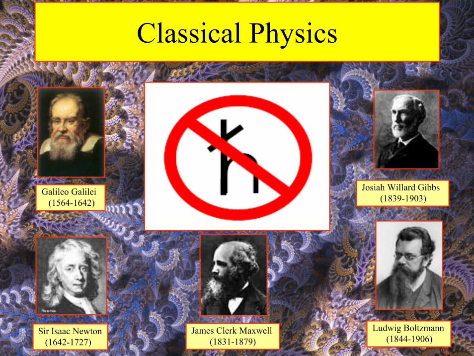
Sir Isaac Newton(1642-1727)

Galileo Galilei(1564-1642)

James Clerk Maxwell(1831-1879)

Josiah Willard Gibbs(1839-1903)

Ludwig Boltzmann(1844-1906)

Classical Physics

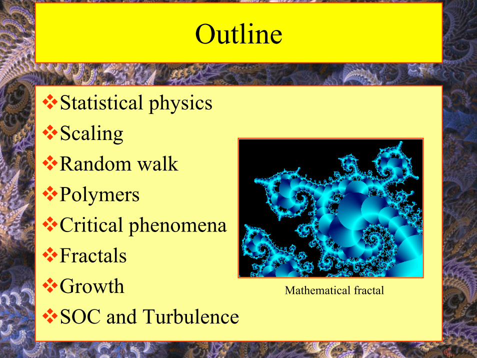
Outline

Statistical physicsScalingRandom walkPolymersCritical phenomenaFractalsGrowthSOC and Turbulence

Mathematical fractal

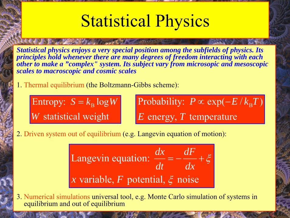
Statistical PhysicsStatistical physics enjoys a very special position among the subfields of physics. Itsprinciples hold whenever there are many degrees of freedom interacting with eachother to make a ”complex" system. Its subject vary from microsopic and mesoscopicscales to macroscopic and cosmic scales

1. Thermal equilibrium (the Boltzmann-Gibbs scheme):

2. Driven system out of equilibrium (e.g. Langevin equation of motion):

3. Numerical simulations universal tool, e.g. Monte Carlo simulation of systems in equilibrium and out of equilibrium

BEntropy: logstatistical weight

S k WW

= BProbability: exp( / ) energy, temperature

P E k TE T

∝ −

Langevin equation:

variable, potential, noise

dx dFdt dx

x F

ξ

ξ

= − +

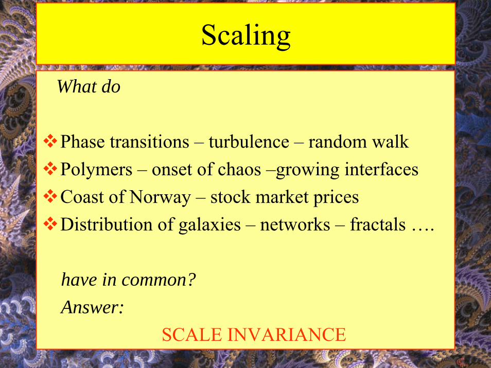
ScalingWhat do

Phase transitions – turbulence – random walkPolymers – onset of chaos –growing interfaces Coast of Norway – stock market pricesDistribution of galaxies – networks – fractals ….

have in common?Answer:

SCALE INVARIANCE

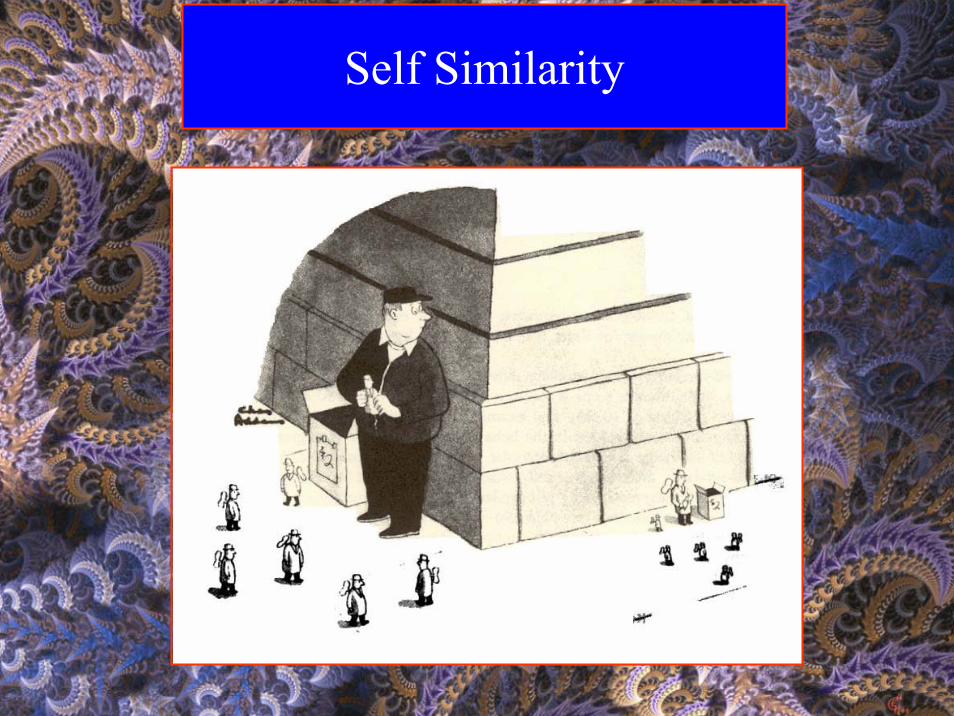
Self Similarity

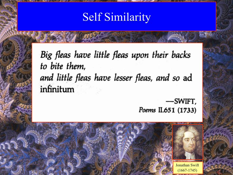
Self Similarity

Jonathan Swift(1667-1745)

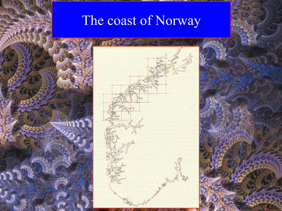
The coast of Norway

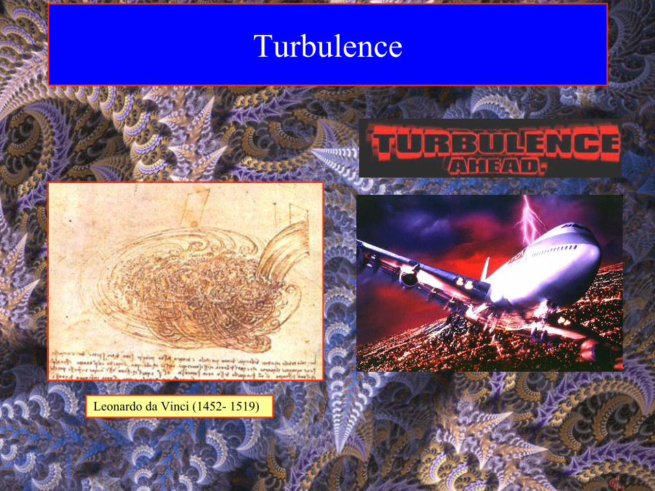
Turbulence

Leonardo da Vinci (1452- 1519)

Polymers

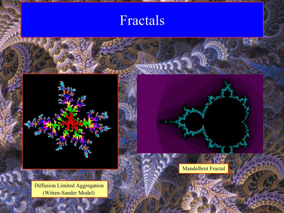
Fractals

Mandelbrot Fractal

Diffusion Limited Aggregation(Witten-Sander Model)

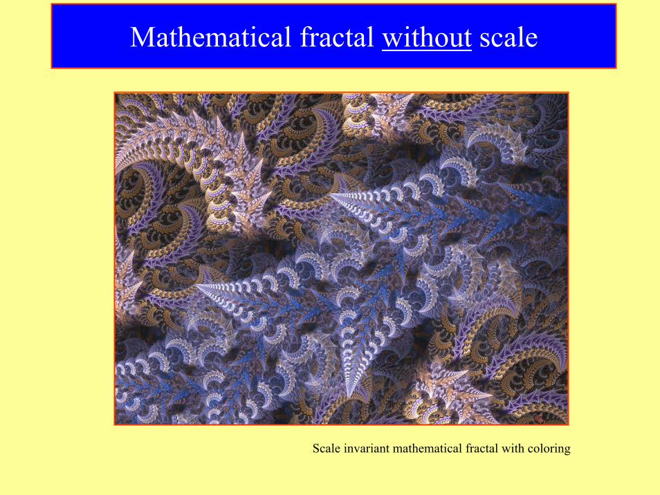
Mathematical fractal without scale

Scale invariant mathematical fractal with coloring

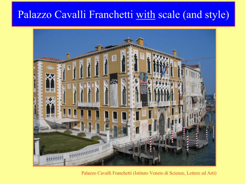
Palazzo Cavalli Franchetti with scale (and style)

Palazzo Cavalli Franchetti (Istituto Veneto di Scienze, Lettere ed Arti)

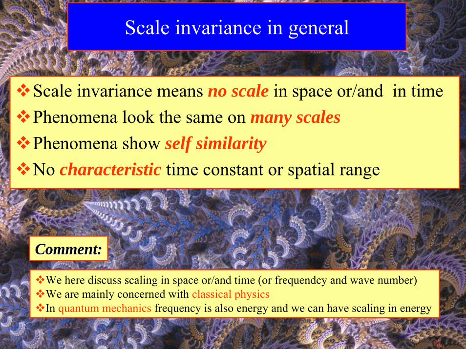
Scale invariance in general

Scale invariance means no scale in space or/and in timePhenomena look the same on many scalesPhenomena show self similarityNo characteristic time constant or spatial range

CommentComment::

We here discuss scaling in space or/and time (or frequendcy and wave number)We are mainly concerned with classical physicsIn quantum mechanics frequency is also energy and we can have scaling in energy

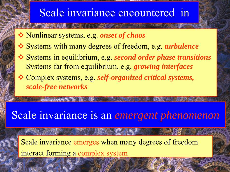
Scale invariance encountered in

Nonlinear systems, e.g. onset of chaosSystems with many degrees of freedom, e.g. turbulenceSystems in equilibrium, e.g. second order phase transitions Systems far from equilibrium, e.g. growing interfacesComplex systems, e.g. self-organized critical systems, scale-free networks

Scale invariance is an emergent phenomenon

Scale invariance emerges when many degrees of freedominteract forming a complex system

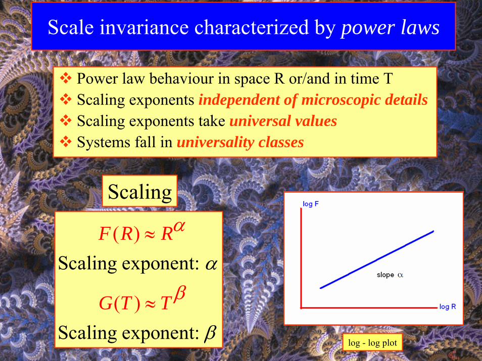
Power law behaviour in space R or/and in time TScaling exponents independent of microscopic detailsScaling exponents take universal valuesSystems fall in universality classes

Scaling exponent

( )

(

:

Scaling expone t

)n :

F R R

G T T

αβ

β

α≈

≈

Scale invariance characterized by power laws

log - log plot

Scaling

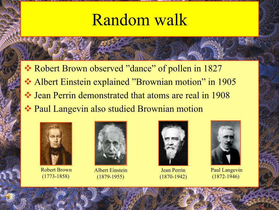
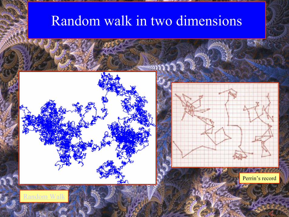
Random walk

Robert Brown observed ”dance” of pollen in 1827Albert Einstein explained ”Brownian motion” in 1905Jean Perrin demonstrated that atoms are real in 1908Paul Langevin also studied Brownian motion

Robert Brown (1773-1858)

Albert Einstein(1879-1955)

Jean Perrin(1870-1942)

Paul Langevin(1872-1946)

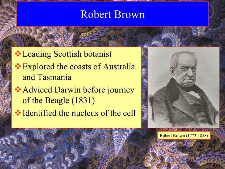
Robert Brown

Leading Scottish botanistExplored the coasts of Australiaand TasmaniaAdviced Darwin before journeyof the Beagle (1831)Identified the nucleus of the cell

Robert Brown (1773-1858)

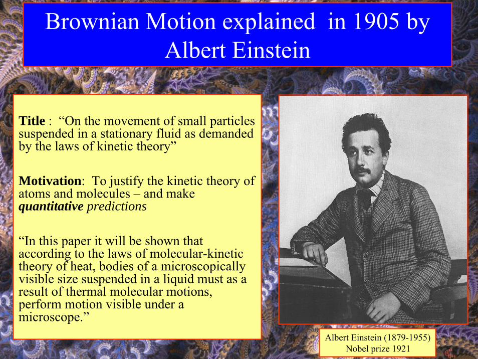
Brownian Motion explained in 1905 by Albert Einstein

Title : “On the movement of small particles suspended in a stationary fluid as demanded by the laws of kinetic theory”

Motivation: To justify the kinetic theory of atoms and molecules – and make quantitative predictions

“In this paper it will be shown that according to the laws of molecular-kinetic theory of heat, bodies of a microscopically visible size suspended in a liquid must as a result of thermal molecular motions, perform motion visible under a microscope.”

Albert Einstein (1879-1955)Nobel prize 1921

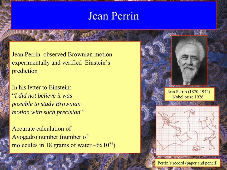
Jean Perrin

Jean Perrin observed Brownian motion experimentally and verified Einstein’sprediction

In his letter to Einstein:“I did not believe it waspossible to study Brownian motion with such precision”

Accurate calculation ofAvogadro number (number ofmolecules in 18 grams of water ~6x1023)

Jean Perrin (1870-1942)Nobel prize 1926

Perrin’s record (paper and pencil)

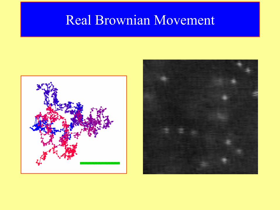
Real Brownian Movement

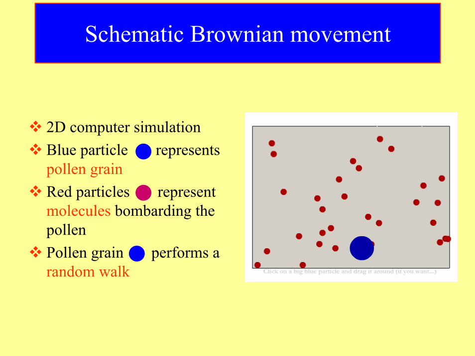
Schematic Brownian movement

2D computer simulationBlue particle representspollen grainRed particles representmolecules bombarding thepollenPollen grain performs a random walk

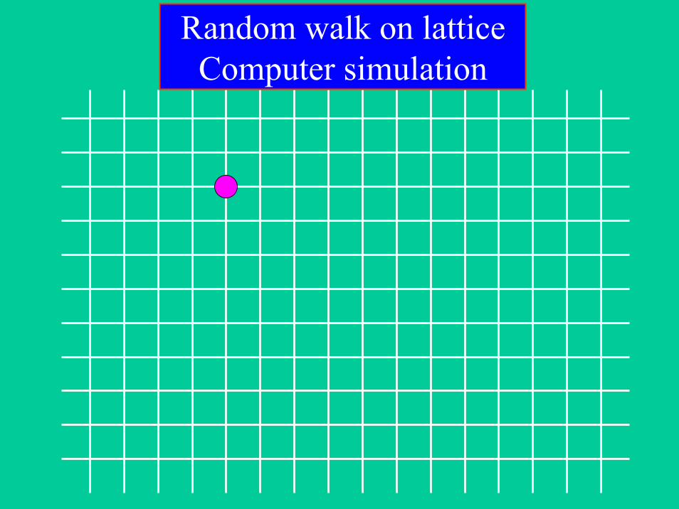
Random walk on latticeComputer simulation

Random walk in two dimensions

Perrin’s record

Random Walk

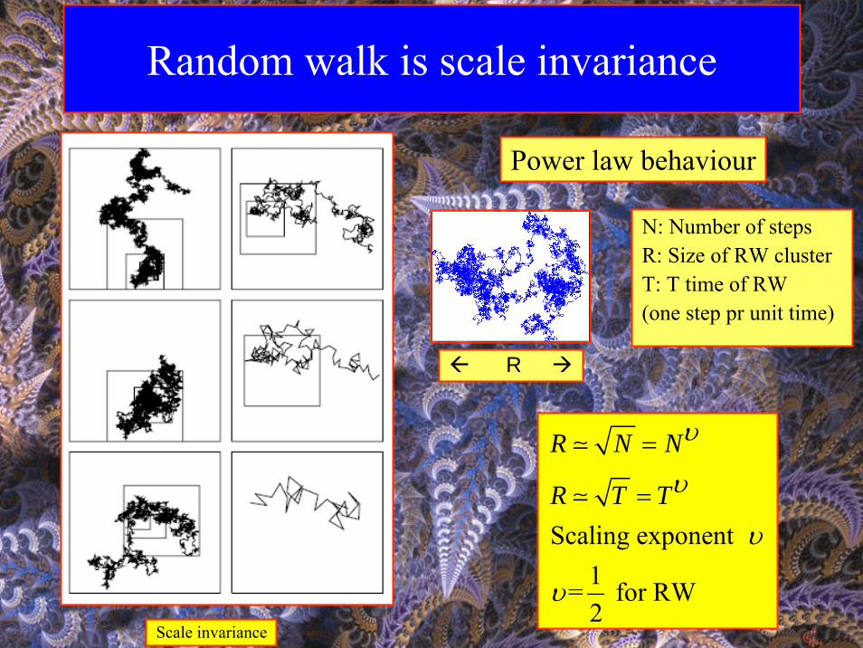
Random walk is scale invariance

N: Number of steps R: Size of RW clusterT: T time of RW (one step pr unit time)

Scale invariance

Power law behaviour

R

Scaling exponent

1 = for RW2

R N N

R T T

υ

υ

υ

υ

=

=

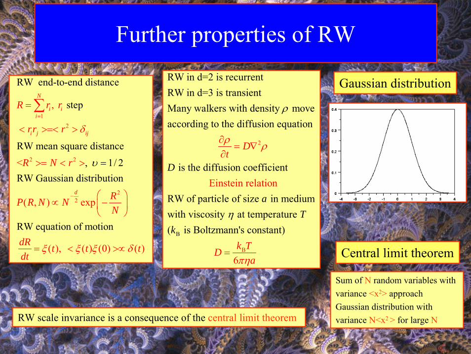
Further properties of RW

12

2 2

22

RW end-to-end distance

step

RW mean square distance , 1/ 2 RW Gaussian distribution

RW equation of motion

,

<

( , ) exp

( ), ( )

N

i ii

i j ij

d

R r r

rr r

R N r

RP R N NN

dR t tdt

ξ

υ

δ

ξ

=

−

=

< >=< >

>= < >

⎛ ⎞∝ −⎜ ⎟

⎝ ⎠

= <

=

∑

(0) ( ) tξ δ>∝

2

RW in d=2 is recurrent RW in d=3 is transientMany walkers with density move according to the diffusion equation

is the diffusion coeff

Eiicient

nstei

Dt

D

ρ

ρ

ρ∂= ∇

∂

B

B

RW of particle of size in medium with viscosity at temperature ( is Boltzmann's constant)

n relation

6

k Tk

a

aT

D

η

πη=

Gaussian distribution

Central limit theorem

Sum of N random variables withvariance <x2> approach Gaussian distribution withvariance N<x2 > for large NRW scale invariance is a consequence of the central limit theorem

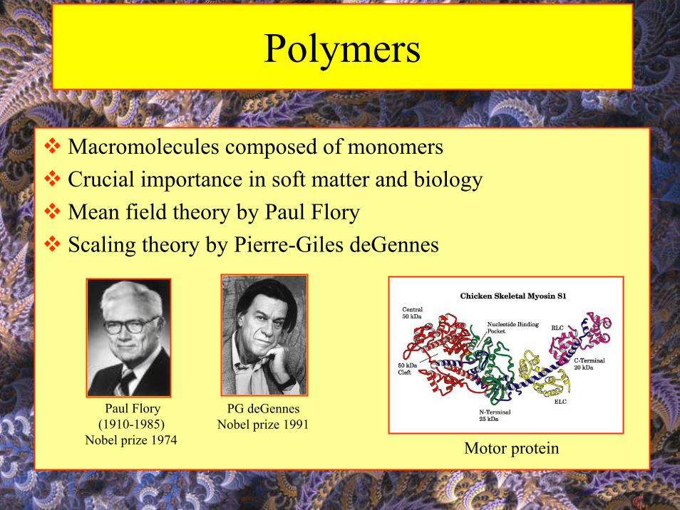
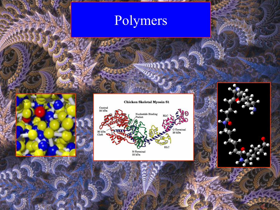
Polymers

Macromolecules composed of monomersCrucial importance in soft matter and biologyMean field theory by Paul FloryScaling theory by Pierre-Giles deGennes

Paul Flory(1910-1985)

Nobel prize 1974

PG deGennesNobel prize 1991

Motor protein

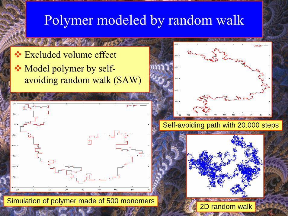
Polymer modeled by random walk

Excluded volume effectModel polymer by self-avoiding random walk (SAW)

Simulation of polymer made of 500 monomers

Self-avoiding path with 20.000 steps

2D random walk

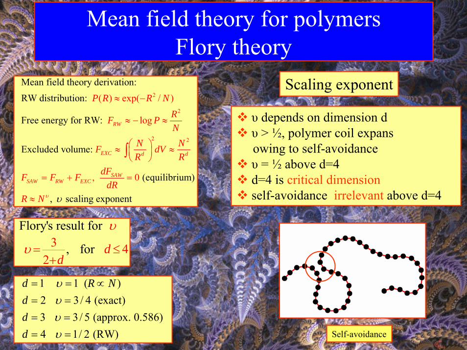
Mean field theory for polymersFlory theory

2

2

2 2

Mean field theory derivation: RW distribution:

Free energy for RW:

Excluded volume:

(equilib

( ) exp( / )

log

, 0 rium)

, sca

RW

EXC d d

SAWSAW RW EXC

P R R NRF PN

N NF dVR R

dFF F FdR

R Nυ υ

≈ −

≈ − ≈

⎛ ⎞≈ ≈⎜ ⎟⎝ ⎠

= + =

≈

∫

ling exponent

Flory's result for

, for 3 4 2

dd

υ

υ = ≤+

1 1 ( ) 2 3 / 4 (exact) 3 3 / 5 (approx. 0.586) 4 1/ 2 (RW)

d R Nddd

υυυυ

= = ∝= == == =

υ depends on dimension dυ > ½, polymer coil expansowing to self-avoidanceυ = ½ above d=4d=4 is critical dimensionself-avoidance irrelevant above d=4

Scaling exponent

Self-avoidance

Critical phenomena

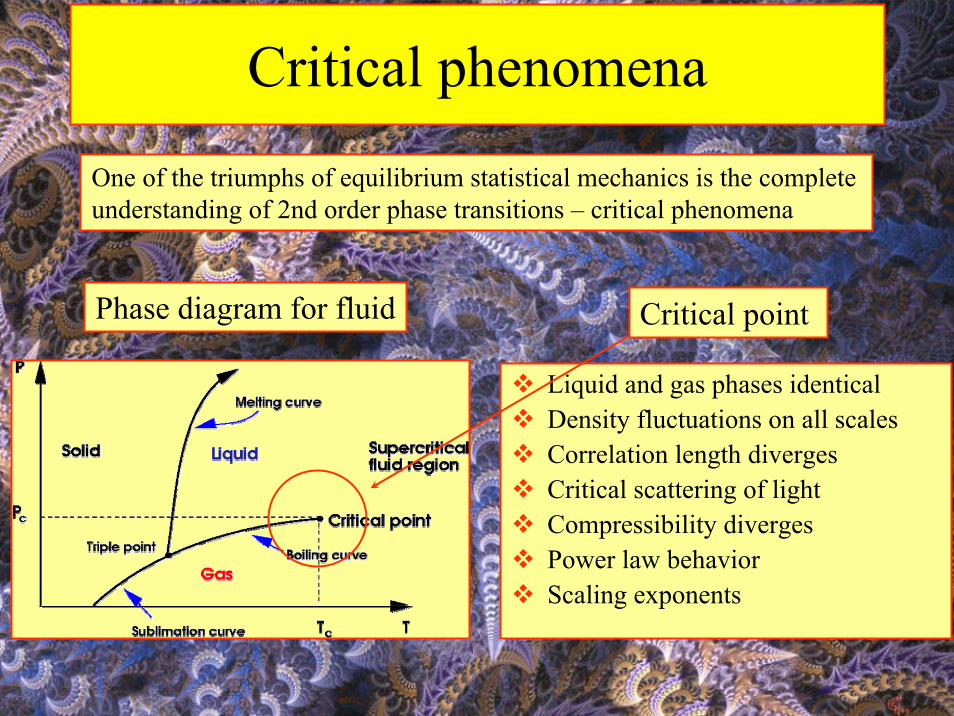
Liquid and gas phases identicalDensity fluctuations on all scalesCorrelation length divergesCritical scattering of light Compressibility divergesPower law behaviorScaling exponents

Critical point Phase diagram for fluid

One of the triumphs of equilibrium statistical mechanics is the completeunderstanding of 2nd order phase transitions – critical phenomena

Basic properties (fluid)

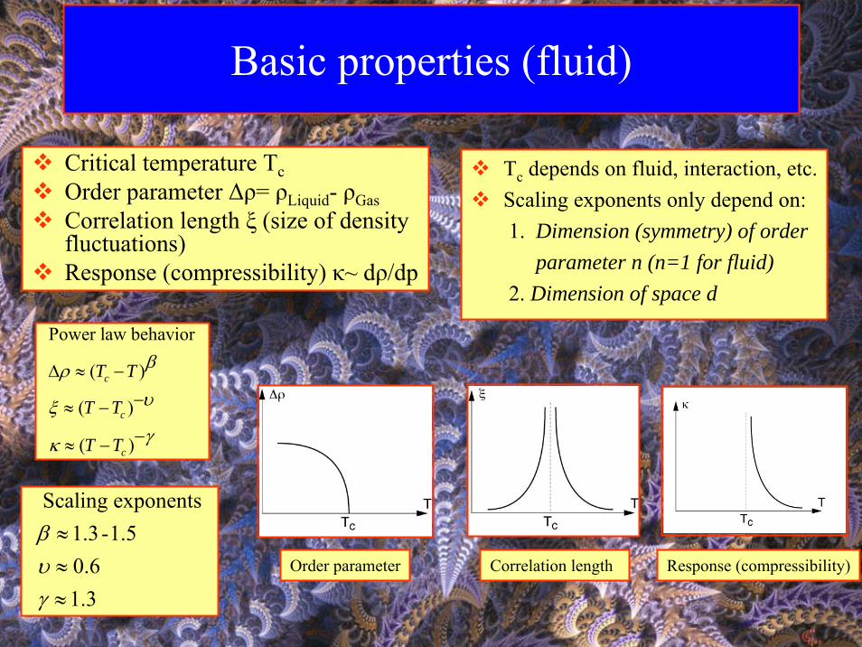
Critical temperature TcOrder parameter Δρ= ρLiquid- ρGasCorrelation length ξ (size of densityfluctuations)Response (compressibility) κ~ dρ/dp

Power law behavior

( )

( )

( )

c

c

c

T T

T T

T T

βρυξγκ

Δ ≈ −

−≈ −

−≈ −

Scaling exponents 1.3-1.5 0.6 1.3

βυγ

≈≈≈

Tc depends on fluid, interaction, etc.Scaling exponents only depend on: 1. Dimension (symmetry) of order

parameter n (n=1 for fluid)2. Dimension of space d

Order parameter Correlation length Response (compressibility)

Ising Model

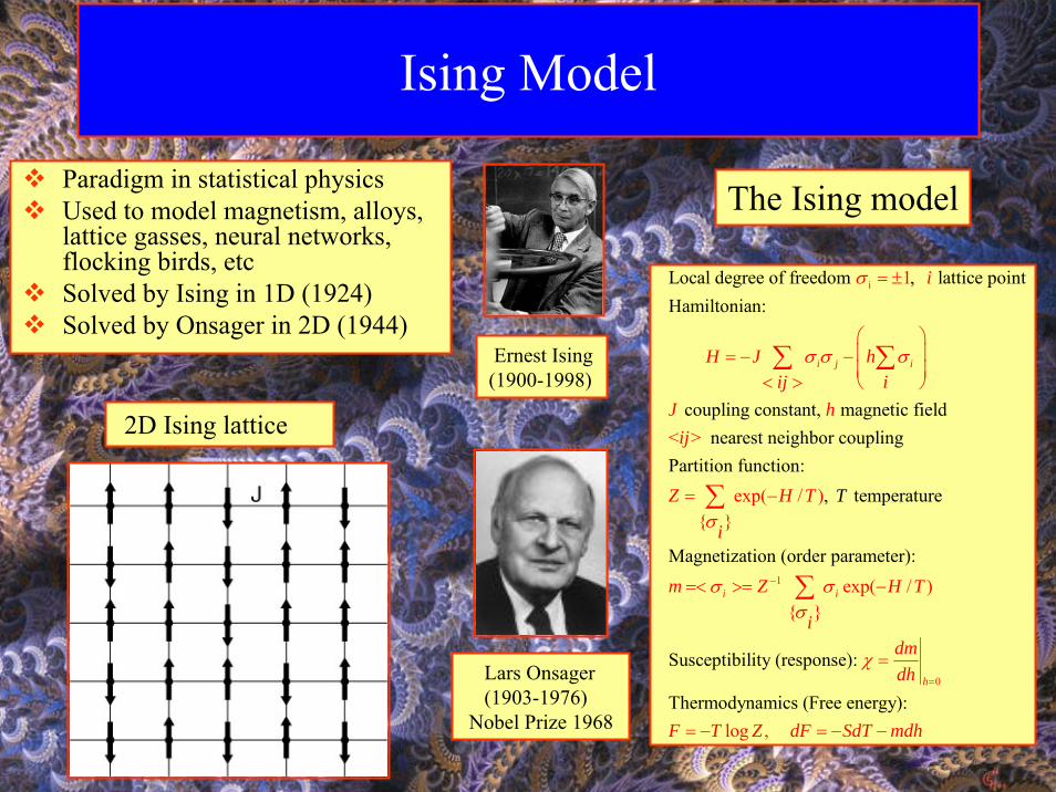
Paradigm in statistical physicsUsed to model magnetism, alloys, lattice gasses, neural networks, flocking birds, etcSolved by Ising in 1D (1924)Solved by Onsager in 2D (1944)

i Local degree of freedom , lattice point Hamiltonian:

coupling constant, magnetic field nearest neighbor coupl

1

< > ing Partition funct

i j i

i

H J hij i

J hij

σ

σ σ σ

= ±

⎛ ⎞⎜ ⎟= − −⎜ ⎟< > ⎝ ⎠

∑ ∑

1

0

ion: , temperature

Magnetization (order parameter):

Susceptibility (response):

Thermodynamics (Free energy):

exp( / ){ }

exp( / ){ }

log ,

i i

h

Z H T

i

m Z H T

idmdh

F T Z d

T

F SdT

σ

σ σσ

χ

−

=

= −

=< >= −

=

= − = − −

∑

∑

mdh

Ernest Ising(1900-1998)

Lars Onsager(1903-1976)

Nobel Prize 1968

The Ising model

2D Ising lattice

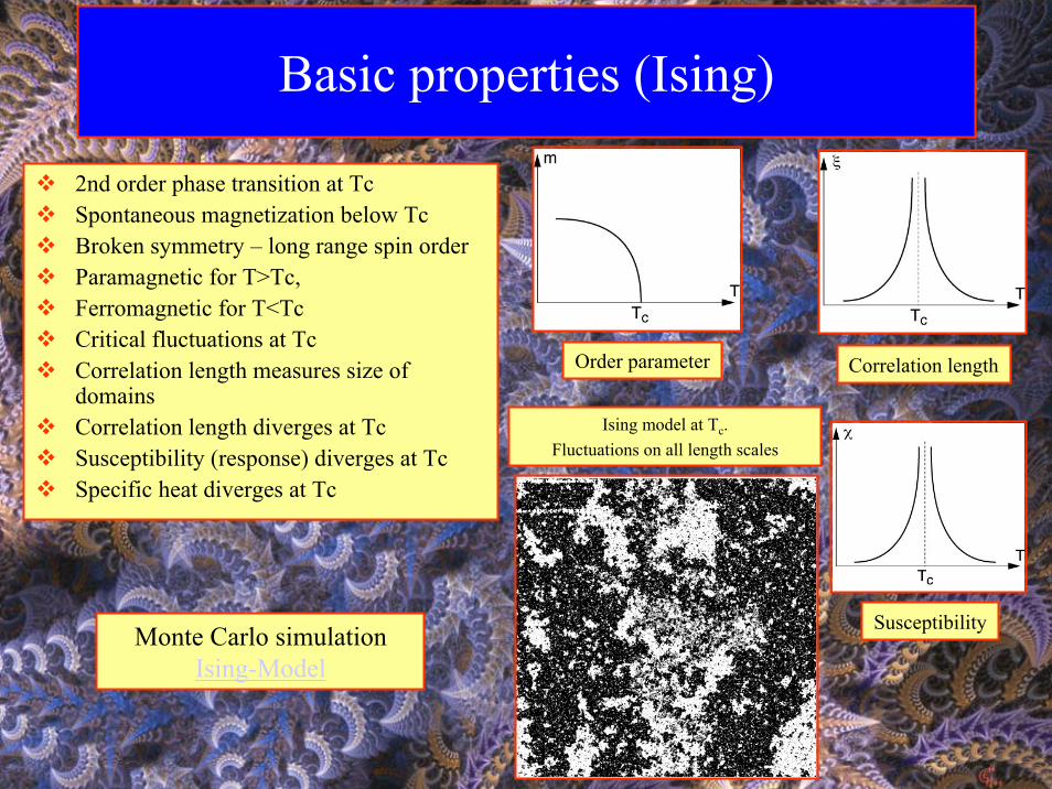
Basic properties (Ising)

2nd order phase transition at TcSpontaneous magnetization below TcBroken symmetry – long range spin orderParamagnetic for T>Tc,Ferromagnetic for T<TcCritical fluctuations at TcCorrelation length measures size ofdomainsCorrelation length diverges at TcSusceptibility (response) diverges at TcSpecific heat diverges at Tc

Monte Carlo simulation Ising-Model

Order parameter Correlation length

Susceptibility

Ising model at Tc. Fluctuations on all length scales

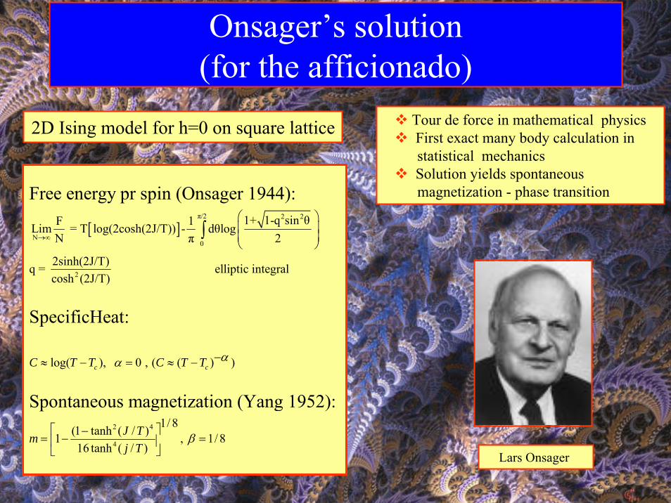
Onsager’s solution(for the afficionado)

[ ]π/2 2 2

N0

2

1+ 1-q sin θF 1 Lim = T log(2cosh(2J/T)) - dθlog N π 2

2sinh(2J/T) q = elliptic integralcosh (2J/T)

log(

Free energy pr spin (Onsager 1944):

SpecificHeat:

C T

→∞

⎛ ⎞⎜ ⎟⎜ ⎟⎝ ⎠

≈ −

∫

2 4

4

), 0 , ( ( ) )

1/ 8(1 tanh ( / ) 1 , 1/ 8

16 tanh ( / )

Spontaneous magnetization (Yang 1952):

c cT C T T

J Tmj T

αα

β

−= ≈ −

⎡ ⎤−= − =⎢ ⎥⎣ ⎦

2D Ising model for h=0 on square lattice

Lars Onsager

Tour de force in mathematical physicsFirst exact many body calculation in statistical mechanicsSolution yields spontaneousmagnetization - phase transition

Brief history of critical phenomena

Second order phase transitions (critical phenomena) ubiquitousMean field theory (MFT) developed early for fluids and magnetsMFT codified by Landau (1937), MFT scaling exponentsExact solution by Onsager of 2D Ising model (1944)Experiments and high-T expansions yield exponents (1960 - 70)Exponents disagree with MFT exponentsUniversality and scaling laws (Widom, Fisher, Josephson)Kadanoff construction (1967)Renormalization group (RG) ideas by Wilson 1963 - 1971RG calculation, critical phenomena ”in the bag” 1971 (Wilson)RG ε-expansion (ε=4 - d) 1972 (Wilson and Fisher)Scaling and RG methods and ideas pervade modern theoretical physics, statistical physics and ”complexity theory”

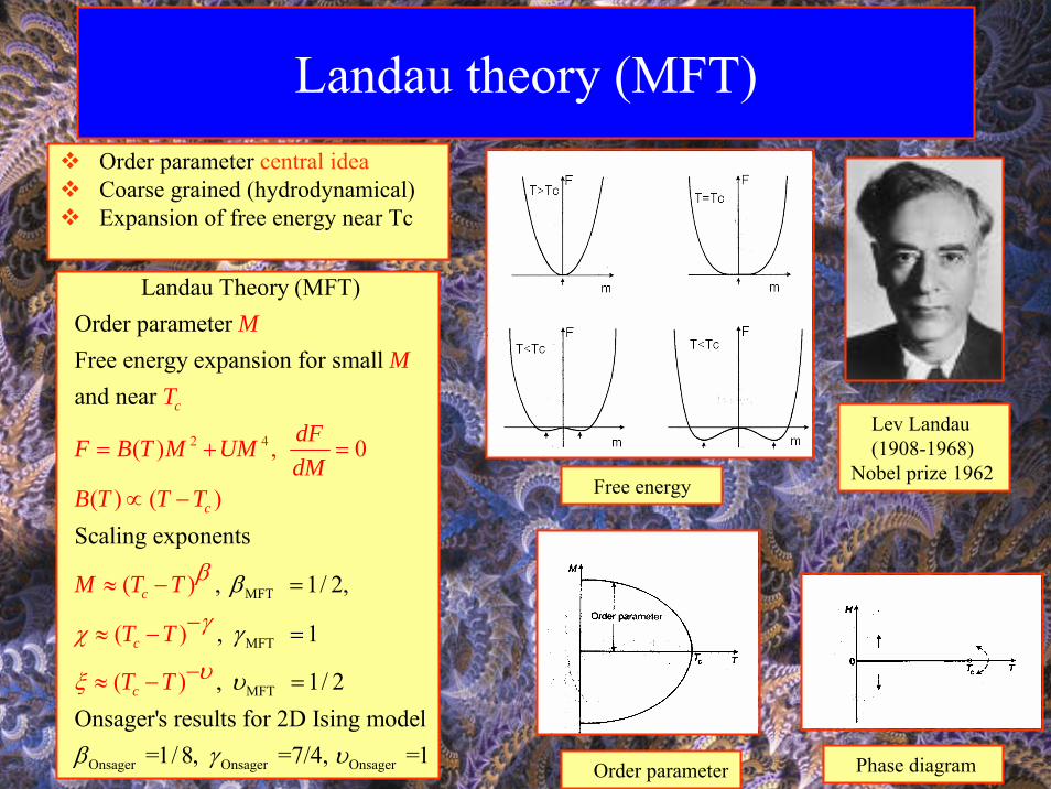
Landau theory (MFT)Order parameter central ideaCoarse grained (hydrodynamical) Expansion of free energy near Tc

MFT

MF

2 4

T

Landau Theory (MFT) Order parameter Free energy expansion for small and near

Scaling exponents

, 1

( )

/ 2,

,

, 0

( ) ( )

( )

(

) 1

c

c

c

c

MM

TdFF B T M UMdM

B T T T

M T T

T T

β

γ

β

γχ

ξ

= + =

∝ −

≈

− =

−

−≈

=

MFT

Onsager Onsager Onsager

, 1/ 2 Onsager's results for 2D Ising model

(

=1/ 8, =7/4 =

)

, 1

cT T υ

β γ υ

υ−− =≈

Free energy

Order parameter

Lev Landau(1908-1968)

Nobel prize 1962

Phase diagram

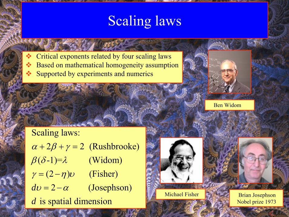
Scaling laws

Critical exponents related by four scaling lawsBased on mathematical homogeneity assumptionSupported by experiments and numerics

Scaling laws: 2 2 (Rushbrooke)

( -1)= (Widom) (2 ) (Fisher) 2 (Josephson)

is spatial dimensiondd

α β γβ δ λγ η υυ α

+ + =

= −= −

Ben Widom

Michael Fisher Brian JosephsonNobel prize 1973

Kadanoff construction I

c

* *

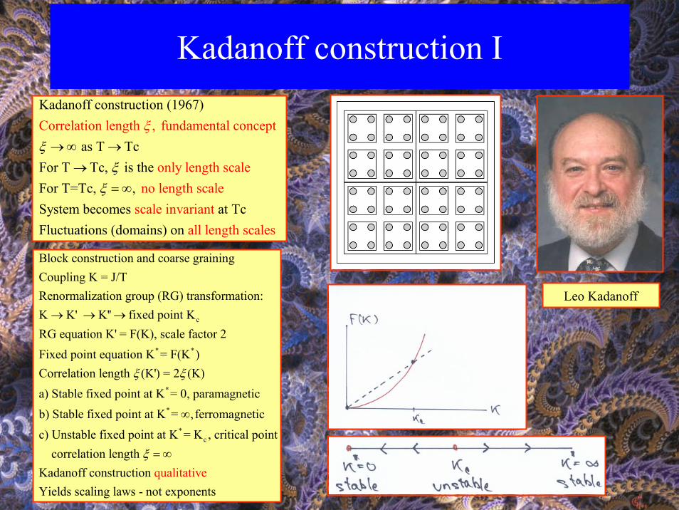
Block construction and coarse graining Coupling K = J/T Renormalization group (RG) transformation: K K' K'' fixed point K RG equation K' = F(K), scale factor 2 Fixed point equation K = F(K ) Corre

→ → →

*

*

*c

lation length (K') = 2 (K) a) Stable fixed point at K = 0, paramagnetic b) Stable fixed point at K = , ferromagnetic c) Unstable fixed point at K = K , critical point correlation length Kada

ξ ξ

ξ

∞

= ∞noff construction

Yields scaling laws - notqualit

exponative

ents

Kadanoff construction (1967)

as T Tc For T Tc, is the For T=Tc,

Correlation length , fundamental concept

only length scaleno length s,

System becomcale

scale invaries an at Tc Flu

t ctuati

ξξ

ξ

ξ→∞ →

→=∞

allons le (doma ngth sins cal) on es

Leo Kadanoff

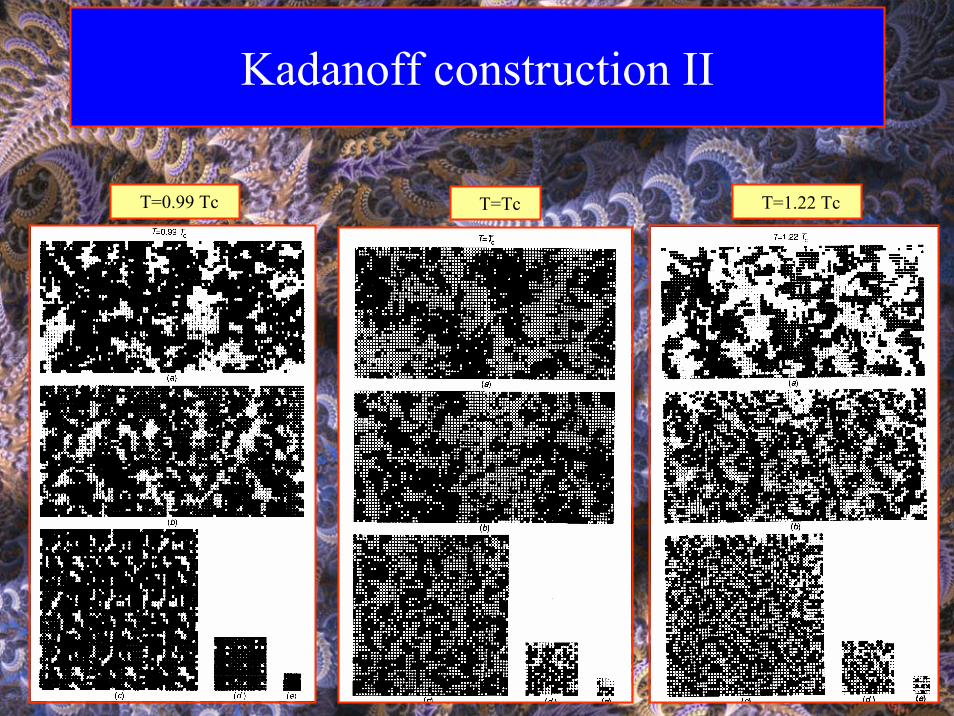
Kadanoff construction II

T=0.99 Tc T=Tc T=1.22 Tc

The Renormalization Group

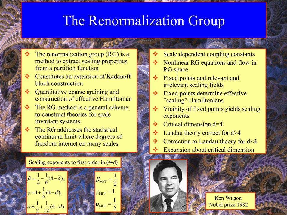
1 1 (4 ), 2 6

11 (4 ),6

1 1 (4 )2 12

d

d

d

β

γ

υ

= − −

= + −

= + −

,,The renormalization group (RG) is a method to extract scaling propertiesfrom a partition functionConstitutes an extension of Kadanoffbloch constructionQuantitative coarse graining and construction of effective HamiltonianThe RG method is a general schemeto construct theories for scaleinvariant systemsThe RG addresses the statisticalcontinuum limit where degrees offreedom interact on many scales

Scale dependent coupling constantsNonlinear RG equations and flow in RG spaceFixed points and relevant and irrelevant scaling fieldsFixed points determine effective”scaling” HamiltoniansVicinity of fixed points yields scalingexponentsCritical dimension d=4Landau theory correct for d>4Correction to Landau theory for d<4Expansion about critical dimension

Scaling exponents to first order in (4-d)

Ken WilsonNobel prize 1982

MFT

MFT

MFT

12

112

β

γ

υ

=

=

=

”Poor man”s RG I

,0 1/

,0 1/ ,1/ 1/

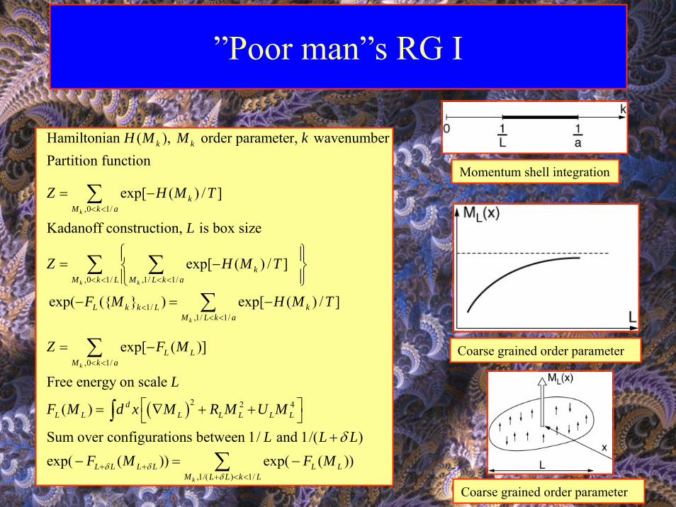
Hamiltonian ( ), order parameter, wavenumber Partition function

exp[ ( ) / ]

Kadanoff construction, is box size

exp[ ( ) / ]

exp(

k

k k

k k

kM k a

kM k L M L k a

H M M k

Z H M T

L

Z H M T

< <

< < < <

= −

⎧ ⎫⎪ ⎪= −⎨ ⎬⎪ ⎪⎩ ⎭

−

∑

∑ ∑

( )

1/,1/ 1/

,0 1/

2 2 4

({ } ) exp[ ( ) / ]

exp[ ( )]

Free energy on scale

( )

Sum over configurations between 1/ and 1/( ) exp( ( ))

k

k

L k k L kM L k a

L LM k a

dL L L L L L L

L L L L

F M H M T

Z F M

L

F M d x M R M U M

L L LF Mδ δ

δ

<< <

< <

+ +

= −

= −

⎡ ⎤= ∇ + +⎣ ⎦+

− =

∑

∑

∫

,1/( ) 1/exp( ( ))

k

L LM L L k L

F Mδ+ < <

−∑

Coarse grained order parameter

Momentum shell integration

Coarse grained order parameter

”Poor man”s RG II

1

2

2 3

2 2

2 / 2 1

31

9 (

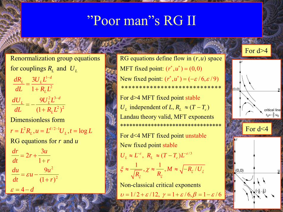
Renormalization group equations for couplings and

D1 )

,imensionless form

RG equations for and

, log

3 21

dL L

Ld

L L

L

d

L L

L L

dR U LdL R L

d

R U

r

U U LdL R L

r L R u L U t L

dr u

u

u

rdt rd

−

−

−

=+

= −+

= = =

= ++

2

2

9(1 )

4

uudt r

d

ε

ε

= −+

= −

( , ) (0,0)(

RG equations define flow in ( , ) space MFT fixed point: New fixed point: ****************************

For d>4 MFT fixed point independent of , (

, ) ( / 6, / 9)

stable)L L c

r ur u

r u

U L R T T

ε ε

∗ ∗

∗ ∗

≈ −

=

= −

/ 3

unstabl

Landau theory valid, MFT exponents*********************************

For d<4 MFT fixed point New fixed point

Non-classical critic

e stable

, ( )1 1

al expo

, , /

n

L L cU L R T T L

M R URR

ε ε

ξ ξξξ

ξ χ

− −≈ ≈ −

≈ ≈ ≈ −

1/ 2 /12, en

1 / 6,ts

1 / 6 υ ε γ ε β ε= + = + = −

For d>4

For d<4

Fractals

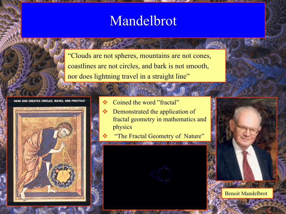
Mandelbrot and Nature"Clouds are not spheres, mountains are not cones,coastlines are not circles, and bark is not smooth,nor does lightning travel in a straight line.“

Mandelbrot 1983

New geometrical description of scale invariant objectsin natural sciences and mathematics

Fractals characterized by non integer dimension

Early history of self similarity

Leibnitz: Recursive self similarityWeierstrass function, ”Monster function”Hilbert and Peano, ”Monster curves”Koch’s curveCantor’s fractal setsPoincare, Klein, Fatou, Julia, Mandelbrot: Iterated functions in the complex planeRichardson: The length of a coast line

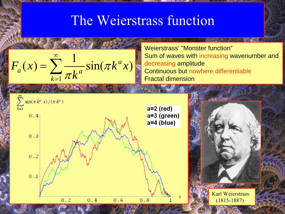
The Weierstrass function

Karl Weierstrass(1815-1887)

1

1( ) sin( )aa a

k

F x k xk

ππ

∞

=

= ∑Weierstrass’ ”Monster function”Sum of waves with increasing wavenumber and decreasing amplitudeContinuous but nowhere differentiableFractal dimension

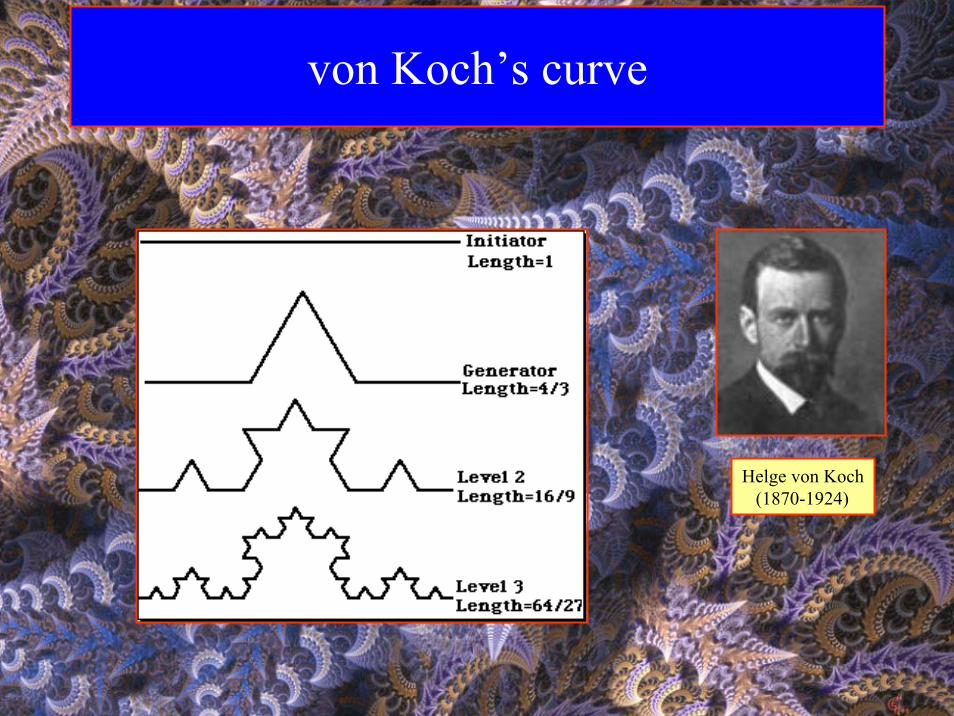
von Koch’s curve

Helge von Koch(1870-1924)

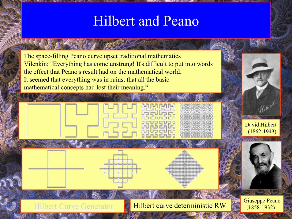
Hilbert and Peano

Hilbert Curve Generator

The space-filling Peano curve upset traditional mathematicsVilenkin: "Everything has come unstrung! It's difficult to put into words the effect that Peano's result had on the mathematical world. It seemed that everything was in ruins, that all the basic mathematical concepts had lost their meaning.“

Hilbert curve deterministic RW

David Hilbert(1862-1943)

Giuseppe Peano(1858-1932)

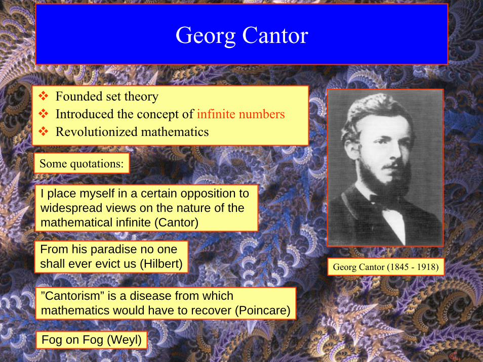
Georg Cantor

Georg Cantor (1845 - 1918)

Founded set theoryIntroduced the concept of infinite numbersRevolutionized mathematics

I place myself in a certain opposition to widespread views on the nature of themathematical infinite (Cantor)

From his paradise no oneshall ever evict us (Hilbert)

”Cantorism” is a disease from whichmathematics would have to recover (Poincare)

Fog on Fog (Weyl)

Some quotations:

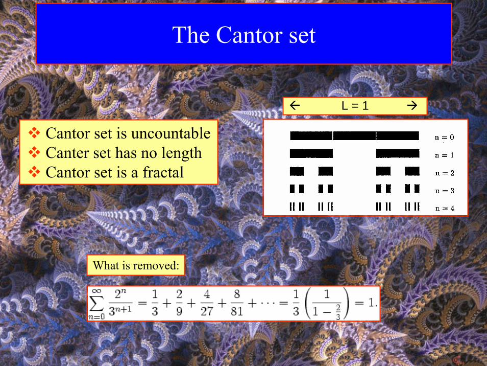
The Cantor set

Cantor set is uncountableCanter set has no lengthCantor set is a fractal

What is removed:

L = 1

Julia sets

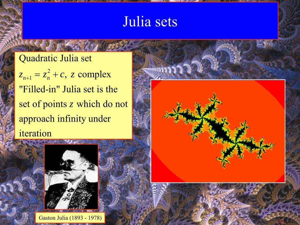
21

Quadratic Julia set , complex "Filled-in" Julia set is the set of points which do not approach infinity under iteration

n nz z c z

z

+ = +

Gaston Julia (1893 - 1978)

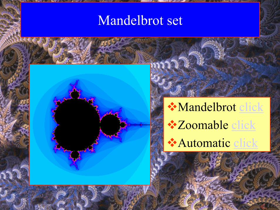
Mandelbrot set

Mandelbrot clickZoomable clickAutomatic click

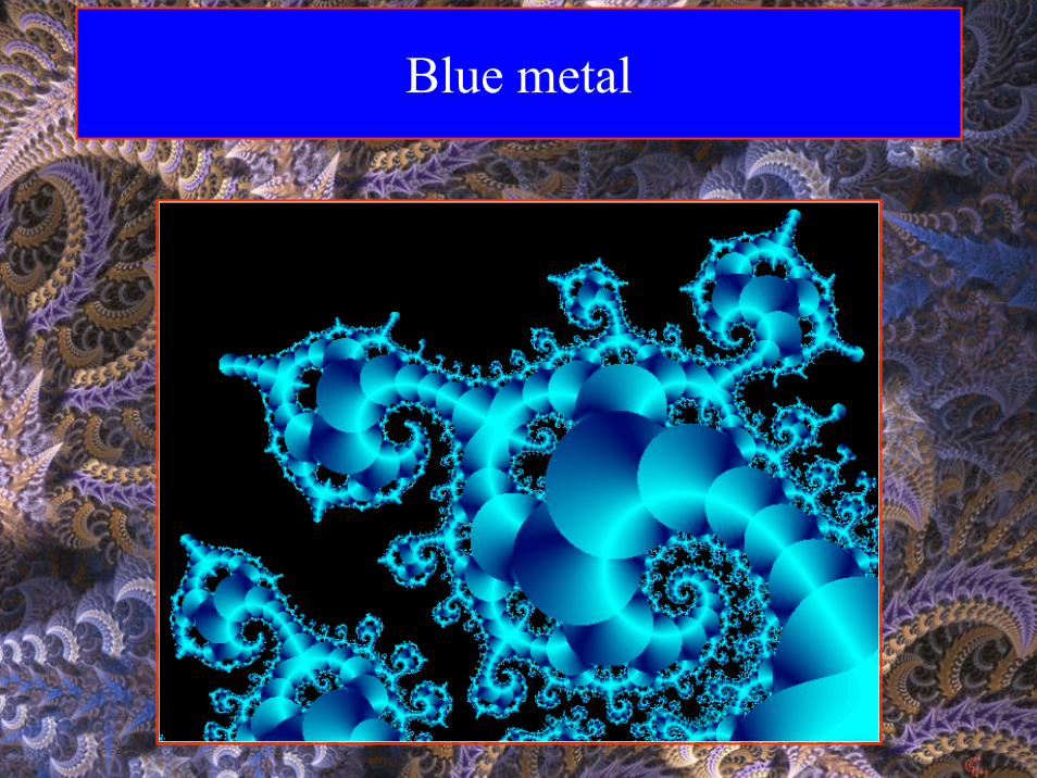
Blue metal

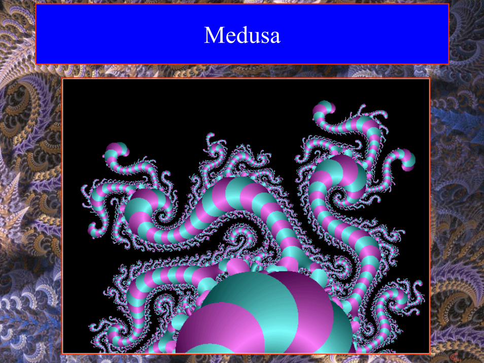
Medusa

Grapes

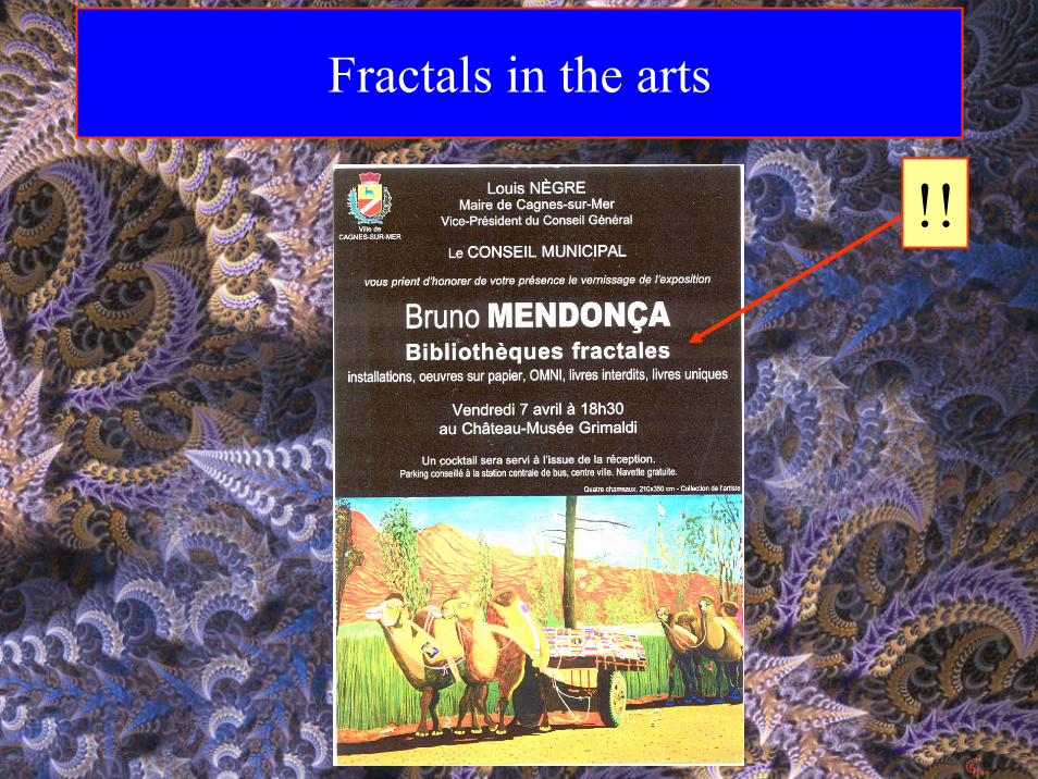
Fractals in the arts

!!

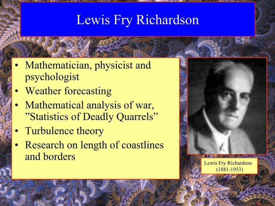
Lewis Fry Richardson

• Mathematician, physicist and psychologist

• Weather forecasting• Mathematical analysis of war,

”Statistics of Deadly Quarrels”• Turbulence theory• Research on length of coastlines

and bordersLewis Fry Richardson

(1881-1953)

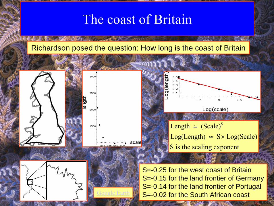
The coast of Britain

Richardson posed the question: How long is the coast of Britain

SLength (Scale)Log(Length) S Log(Scale)S is the scaling exponent

×

S=-0.25 for the west coast of BritainS=-0.15 for the land frontier of GermanyS=-0.14 for the land frontier of PortugalS=-0.02 for the South African coastGoogle Earth

Mandelbrot

“Clouds are not spheres, mountains are not cones,coastlines are not circles, and bark is not smooth,nor does lightning travel in a straight line”

Benoit Mandelbrot

Coined the word ”fractal” Demonstrated the application offractal geometry in mathematics and physics“The Fractal Geometry of Nature”

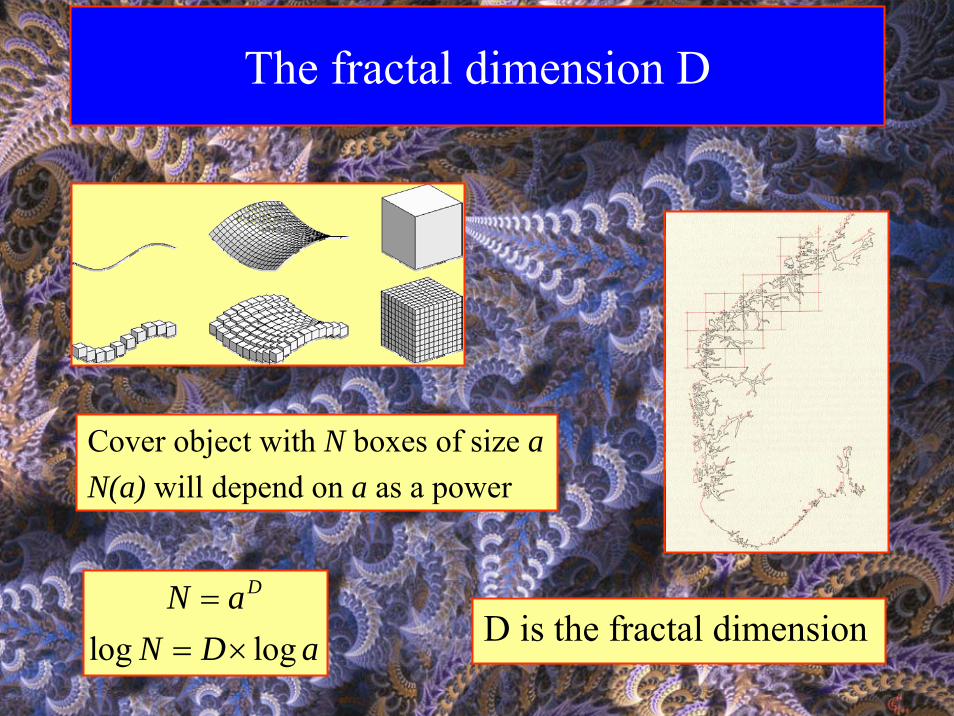
The fractal dimension D

Cover object with N boxes of size aN(a) will depend on a as a power

log log

DN aN D a

== × D is the fractal dimension

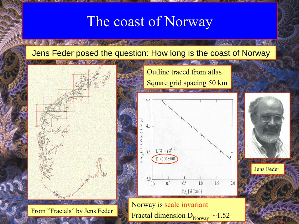
The coast of Norway

Jens Feder posed the question: How long is the coast of Norway

Outline traced from atlasSquare grid spacing 50 km

From ”Fractals” by Jens FederNorway is scale invariantFractal dimension DNorway ~1.52

Jens Feder

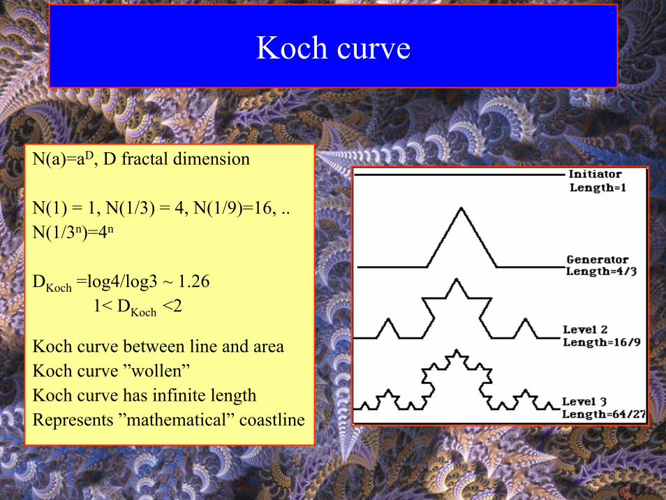
Koch curve

N(a)=aD, D fractal dimension

N(1) = 1, N(1/3) = 4, N(1/9)=16, ..N(1/3n)=4n

DKoch =log4/log3 ~ 1.261< DKoch <2

Koch curve between line and areaKoch curve ”wollen”Koch curve has infinite lengthRepresents ”mathematical” coastline

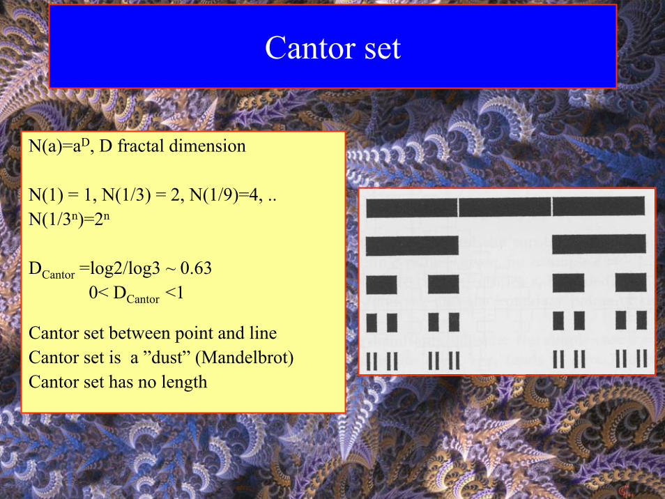
Cantor set

N(a)=aD, D fractal dimension

N(1) = 1, N(1/3) = 2, N(1/9)=4, ..N(1/3n)=2n

DCantor =log2/log3 ~ 0.630< DCantor <1

Cantor set between point and lineCantor set is a ”dust” (Mandelbrot)Cantor set has no length

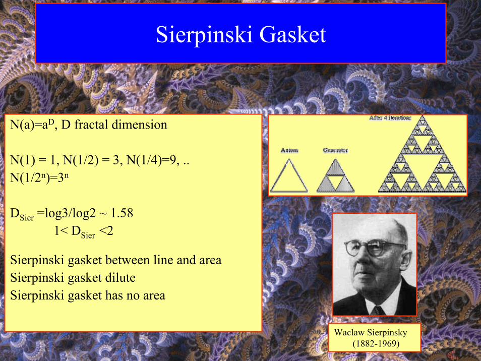
Sierpinski Gasket

N(a)=aD, D fractal dimension

N(1) = 1, N(1/2) = 3, N(1/4)=9, ..N(1/2n)=3n

DSier =log3/log2 ~ 1.581< DSier <2

Sierpinski gasket between line and areaSierpinski gasket diluteSierpinski gasket has no area

Waclaw Sierpinsky(1882-1969)

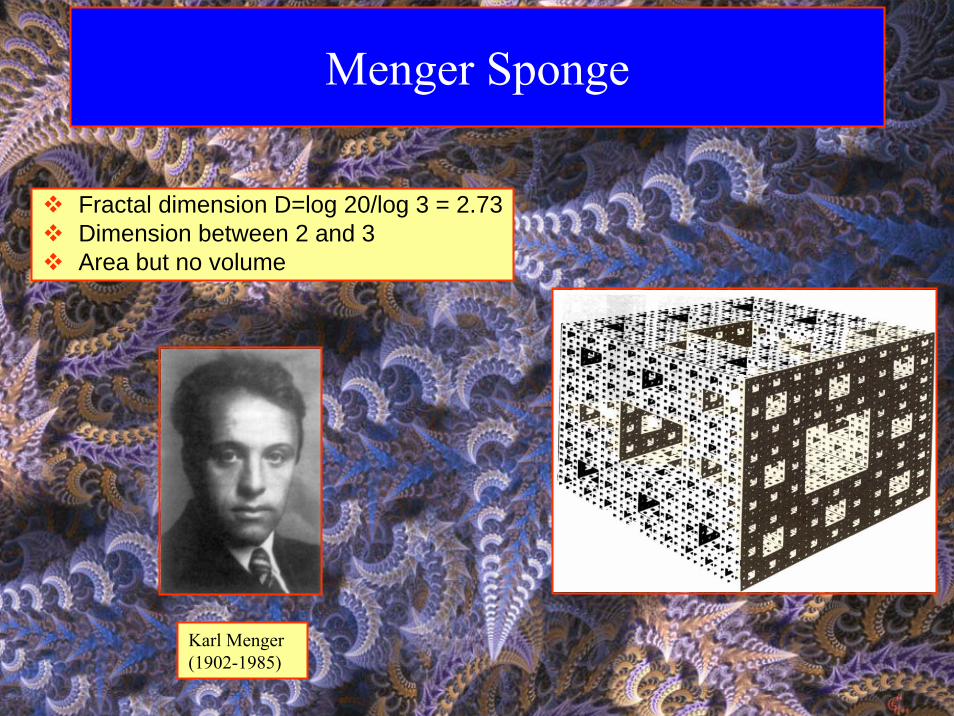
Menger Sponge

Fractal dimension D=log 20/log 3 = 2.73Dimension between 2 and 3Area but no volume

Karl Menger(1902-1985)

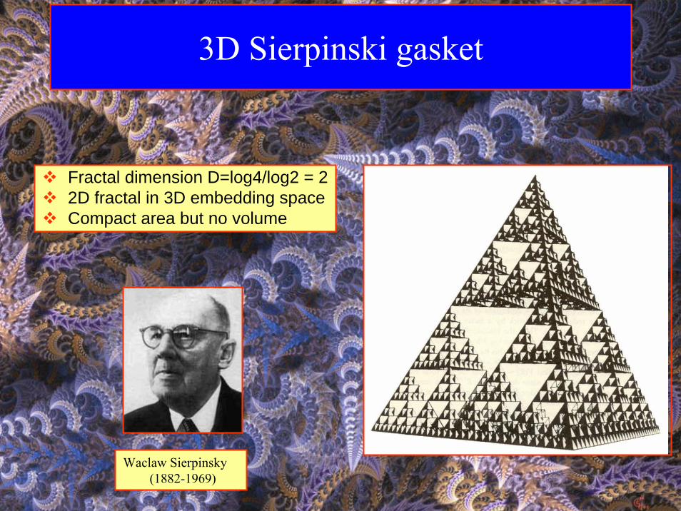
3D Sierpinski gasket

Fractal dimension D=log4/log2 = 22D fractal in 3D embedding spaceCompact area but no volume

Waclaw Sierpinsky(1882-1969)

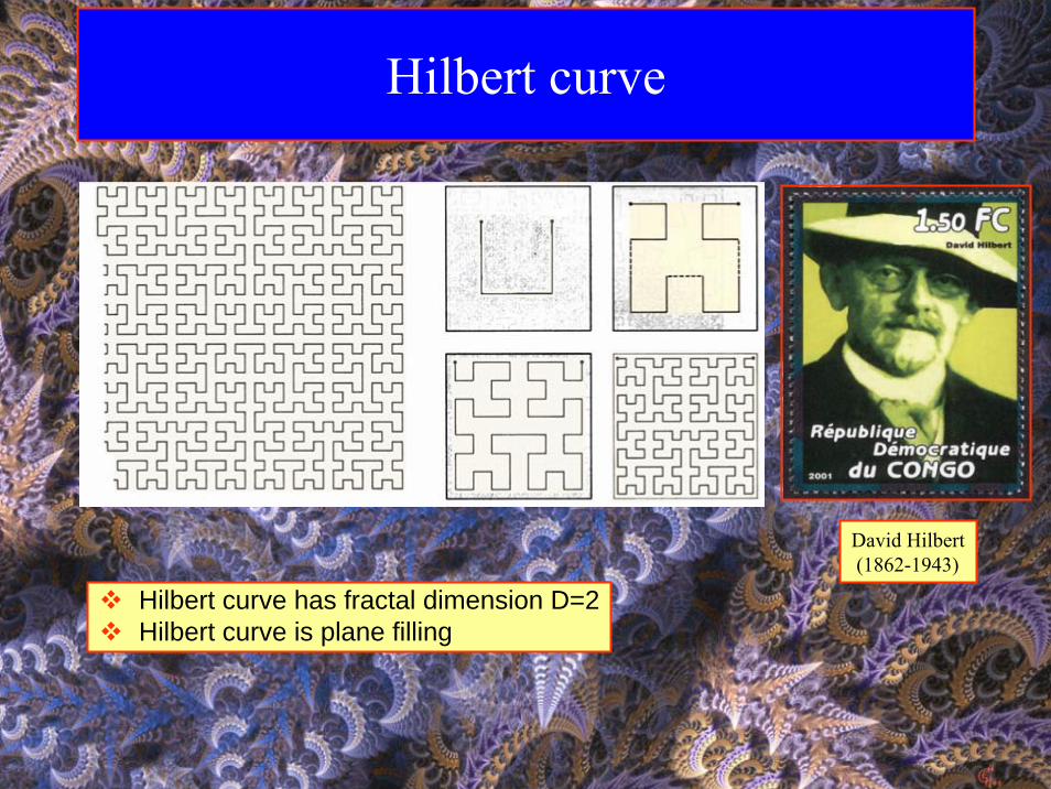
Hilbert curve

Hilbert curve has fractal dimension D=2Hilbert curve is plane filling

David Hilbert(1862-1943)

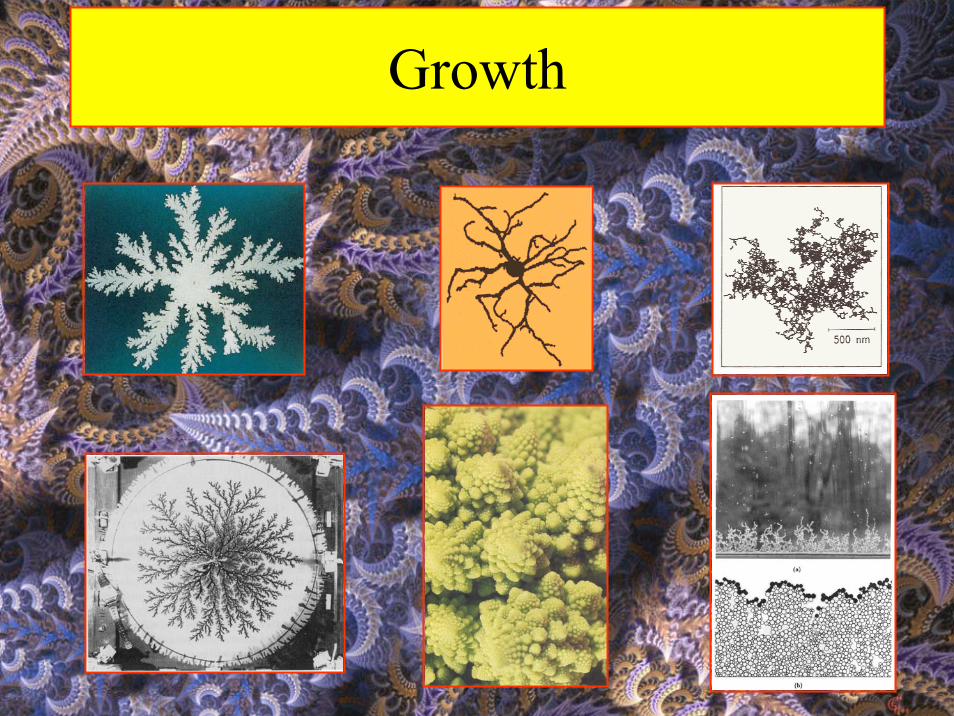
Growth

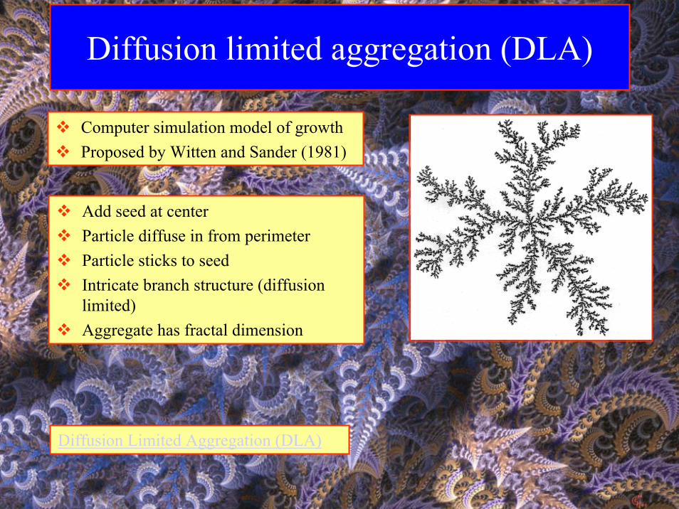
Diffusion Limited Aggregation (DLA)

Computer simulation model of growthProposed by Witten and Sander (1981)

Add seed at centerParticle diffuse in from perimeterParticle sticks to seedIntricate branch structure (diffusion limited)Aggregate has fractal dimension

Diffusion limited aggregation (DLA)

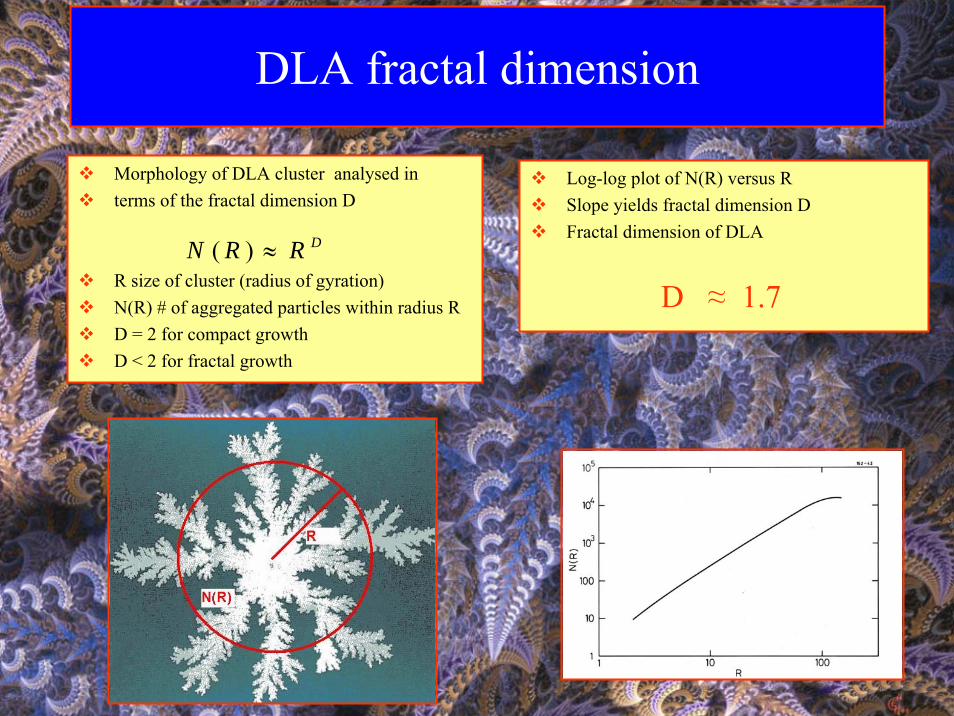
DLA fractal dimension

Log-log plot of N(R) versus RSlope yields fractal dimension DFractal dimension of DLA

D ≈ 1.7

Morphology of DLA cluster analysed in terms of the fractal dimension D

R size of cluster (radius of gyration)N(R) # of aggregated particles within radius RD = 2 for compact growthD < 2 for fractal growth

( ) DN R R≈

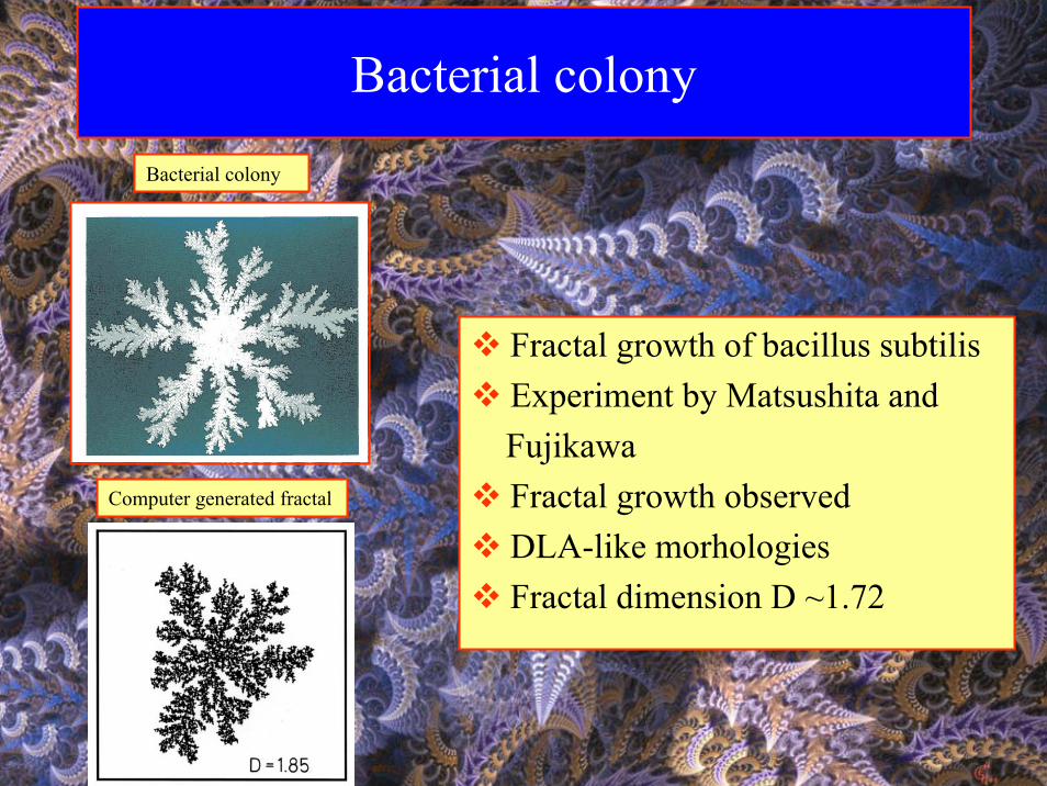
Bacterial colony

Fractal growth of bacillus subtilisExperiment by Matsushita and FujikawaFractal growth observedDLA-like morhologiesFractal dimension D ~1.72

Bacterial colony

Computer generated fractal

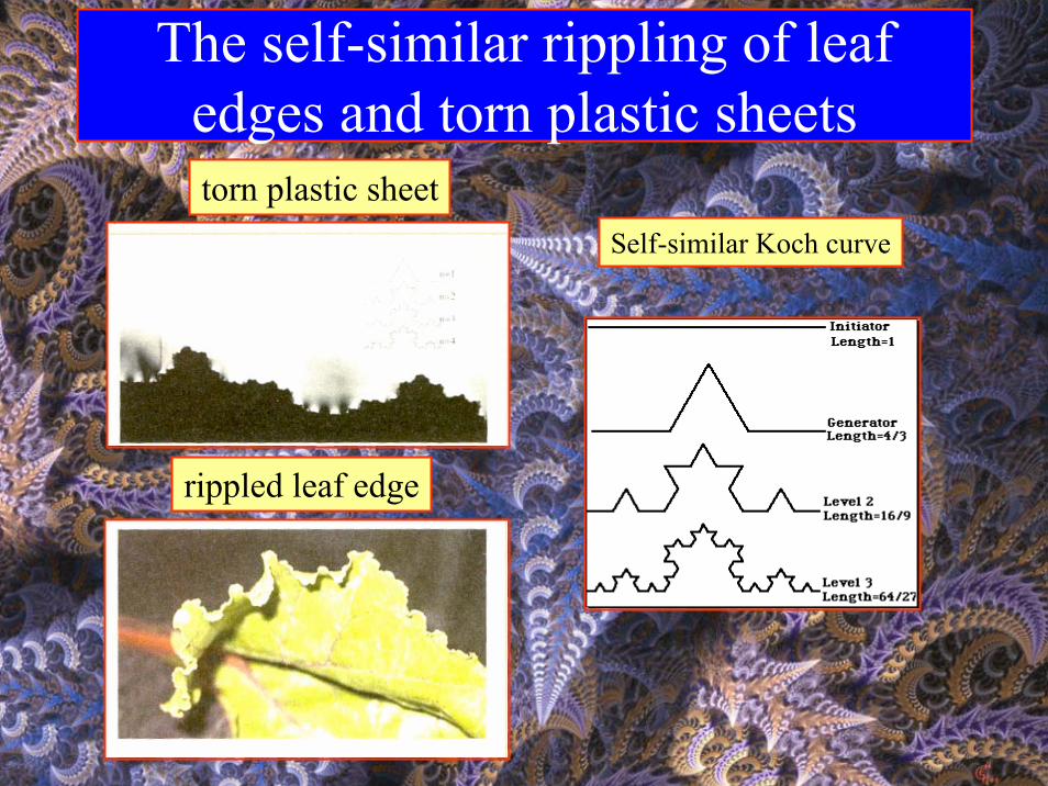
The self-similar rippling of leafedges and torn plastic sheets

Self-similar Koch curve

torn plastic sheet

rippled leaf edge

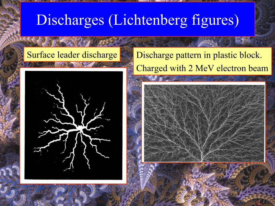
Discharges (Lichtenberg figures)

Surface leader discharge Discharge pattern in plastic block. Charged with 2 MeV electron beam

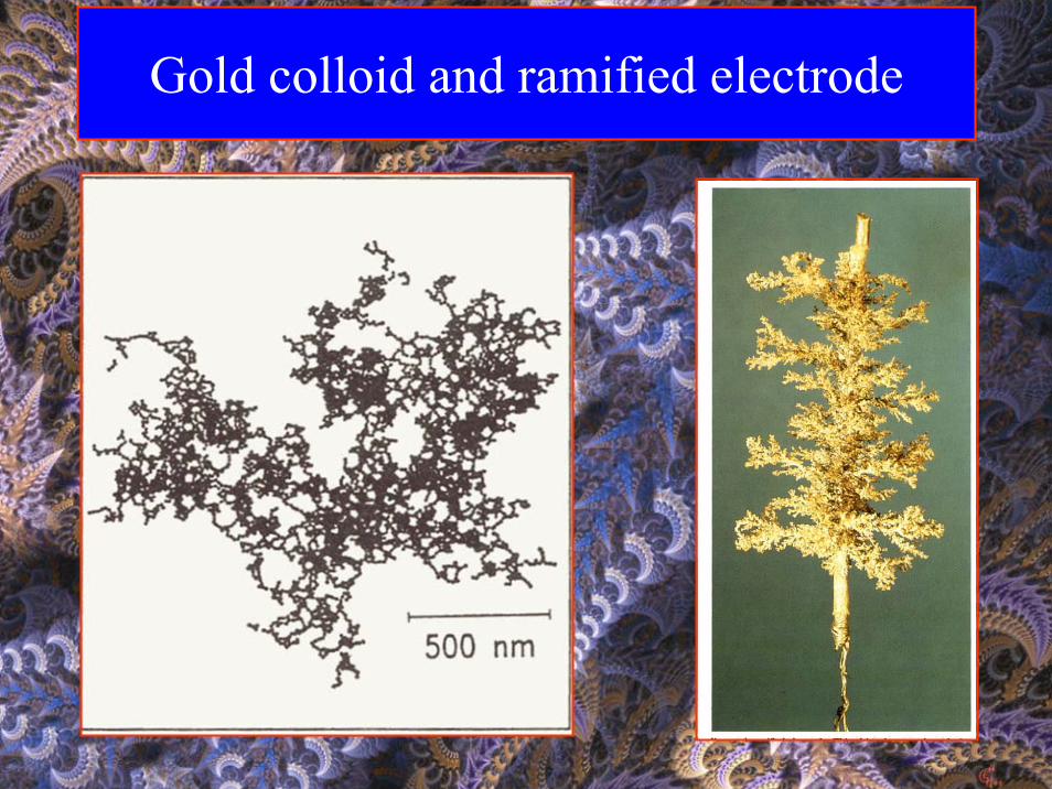
Gold colloid and ramified electrode

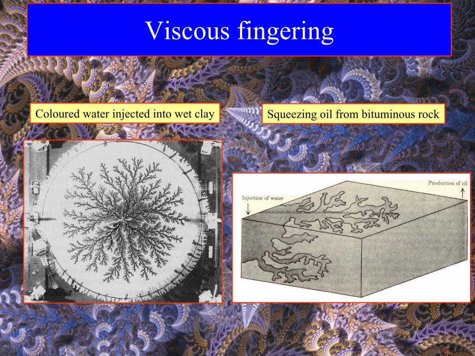
Viscous fingering

Coloured water injected into wet clay Squeezing oil from bituminous rock

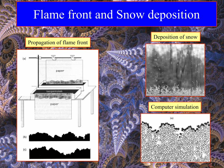
Flame front and Snow deposition

Propagation of flame frontDeposition of snow

Computer simulation

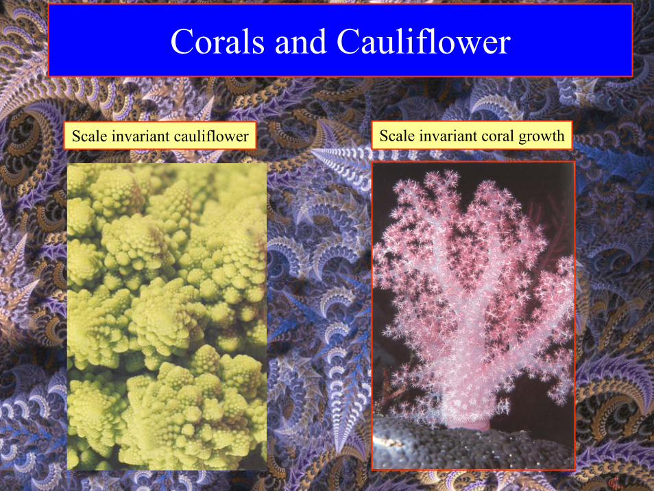
Corals and Cauliflower

Scale invariant cauliflower Scale invariant coral growth

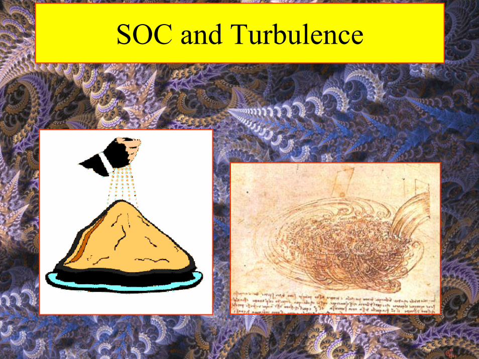
SOC and Turbulence

Self-Organized Criticality (SOC I)

One of the founders and most influential contributors to the study of complex systems. Per Bak made many contributions to science, but the best known was a general theory ofself-organization, which he called, "self-organized criticality". His ideas and discoverieshave had an influence over how people think about a broad range of phenomena, from physics to biology, neurosciences, cosmology, earth sciences, economics and beyond.

Per Bak (1947-2002)

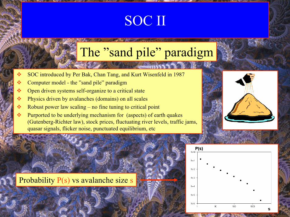
SOC II

SOC introduced by Per Bak, Chan Tang, and Kurt Wisenfeld in 1987Computer model - the ”sand pile” paradigmOpen driven systems self-organize to a critical statePhysics driven by avalanches (domains) on all scalesRobust power law scaling – no fine tuning to critical pointPurported to be underlying mechanism for (aspects) of earth quakes(Gutenberg-Richter law), stock prices, fluctuating river levels, traffic jams, quasar signals, flicker noise, punctuated equilibrium, etc

The ”sand pile” paradigm

Probability P(s) vs avalanche size s

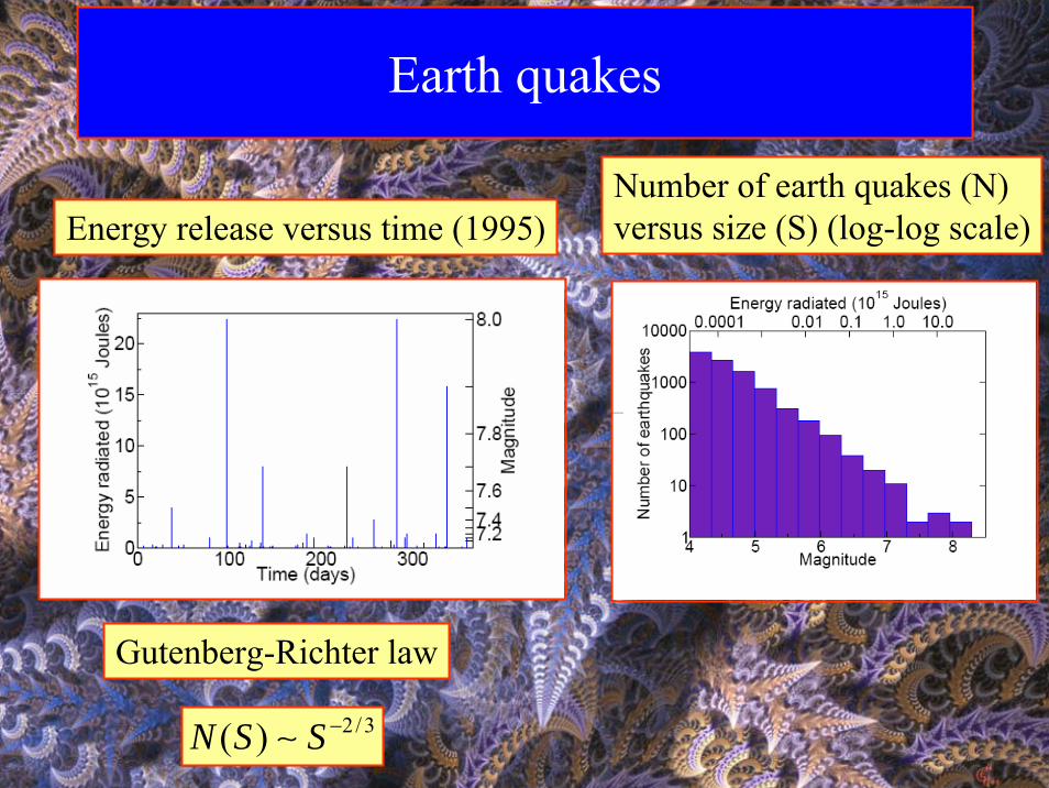
Earth quakes

Energy release versus time (1995)Number of earth quakes (N)versus size (S) (log-log scale)

Gutenberg-Richter law

2/3( )N S S −∼

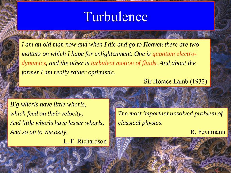
Turbulence

I am an old man now and when I die and go to Heaven there are two matters on which I hope for enlightenment. One is quantum electro-dynamics, and the other is turbulent motion of fluids. And about the former I am really rather optimistic.

Sir Horace Lamb (1932)

Big whorls have little whorls, which feed on their velocity, And little whorls have lesser whorls, And so on to viscosity.

L. F. Richardson

The most important unsolved problem ofclassical physics.

R. Feynmann

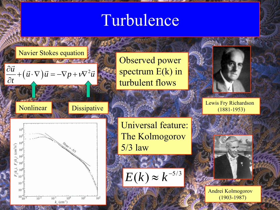
Turbulence

( ) 2u u u p ut

ν∂+ ⋅∇ = −∇ + ∇

∂

Andrei Kolmogorov(1903-1987)

Lewis Fry Richardson(1881-1953)

3/5)( −≈ kkE

Navier Stokes equation

Universal feature:The Kolmogorov5/3 law

Observed power spectrum E(k) in turbulent flows

Nonlinear Dissipative

The end