1

SCALE UP VS. SCALE OUT IN CLOUD STORAGE AND GRAPH PROCESSING SYSTEMSWenting Wang

Le Xu

Indranil Gupta

Department of Computer Science, University of Illinois, Urbana Champaign

2

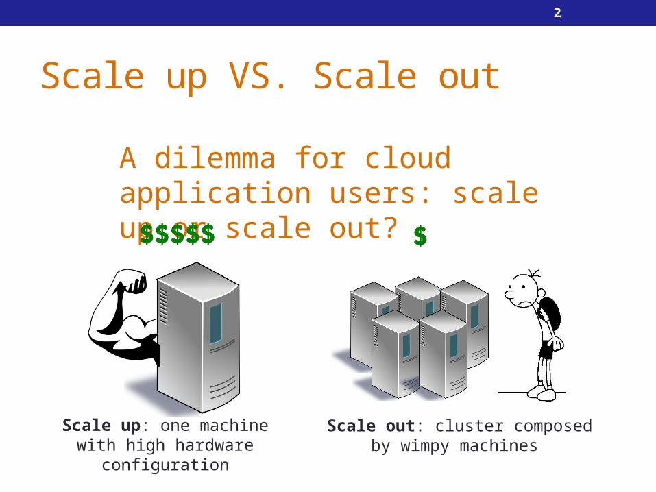
Scale up VS. Scale out

A dilemma for cloud application users: scale up or scale out?

Scale up: one machine with high hardware configuration

Scale out: cluster composed by wimpy machines

3

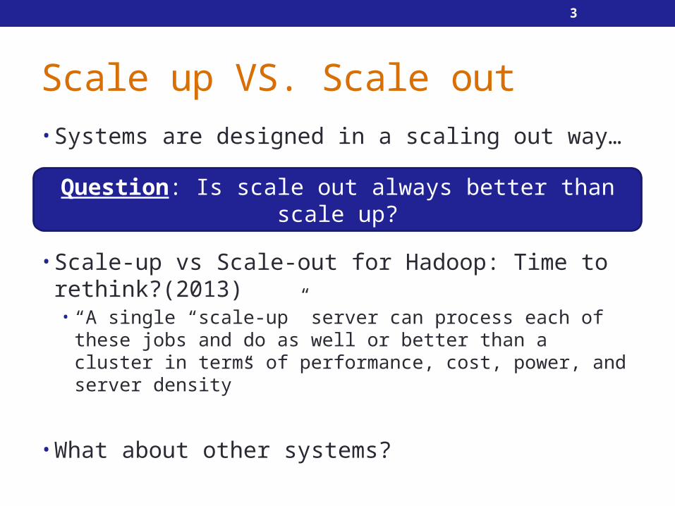
Scale up VS. Scale out• Systems are designed in a scaling out way…

• Scale-up vs Scale-out for Hadoop: Time to rethink?(2013)• “A single “scale-up” server can process each of these jobs and do

as well or better than a cluster in terms of performance, cost, power, and server density”

• What about other systems?

Question: Is scale out always better than scale up?

4

Contributions• Set up pricing models using public cloud pricing scheme

• Linear Square fit on CPU, Memory and Storage• Estimation for arbitrary configuration

• Provide deployment guidance for users with dollar budget caps or minimum throughput requirements in homogeneous environment• Apache Cassandra, the most popular open-source distributed key-

value store• GraphLab, a popular open-source distributed graph processing

system

5

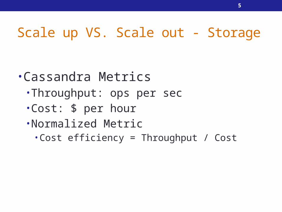
Scale up VS. Scale out - Storage

• Cassandra Metrics• Throughput: ops per sec• Cost: $ per hour• Normalized Metric

• Cost efficiency = Throughput / Cost

6

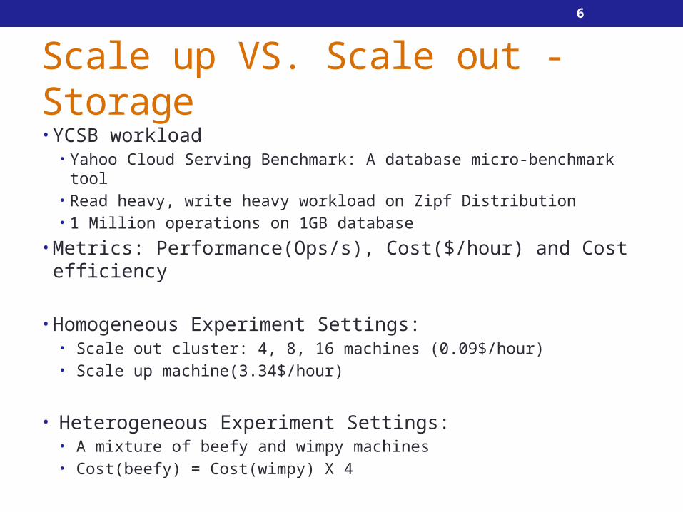
Scale up VS. Scale out - Storage• YCSB workload

• Yahoo Cloud Serving Benchmark: A database micro-benchmark tool• Read heavy, write heavy workload on Zipf Distribution• 1 Million operations on 1GB database

• Metrics: Performance(Ops/s), Cost($/hour) and Cost efficiency

• Homogeneous Experiment Settings: • Scale out cluster: 4, 8, 16 machines (0.09$/hour)• Scale up machine(3.34$/hour)

• Heterogeneous Experiment Settings: • A mixture of beefy and wimpy machines• Cost(beefy) = Cost(wimpy) X 4

7

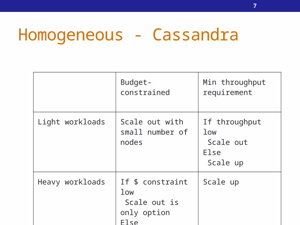
Homogeneous - Cassandra

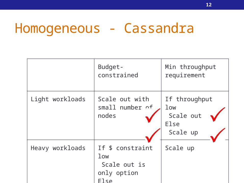
Budget-constrained Min throughput requirement

Light workloads Scale out withsmall number of nodes

If throughput low Scale outElse Scale up

Heavy workloads If $ constraint low Scale out is only option Else Scale up

Scale up

8

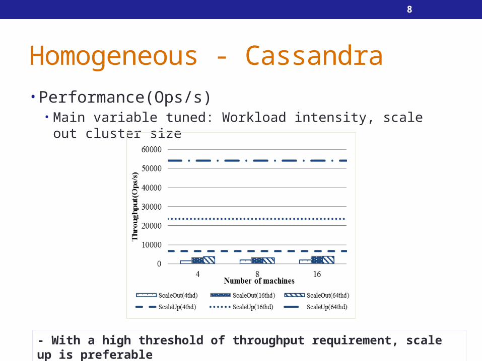
Homogeneous - Cassandra• Performance(Ops/s)

• Main variable tuned: Workload intensity, scale out cluster size

- With a high threshold of throughput requirement, scale up is preferable

9

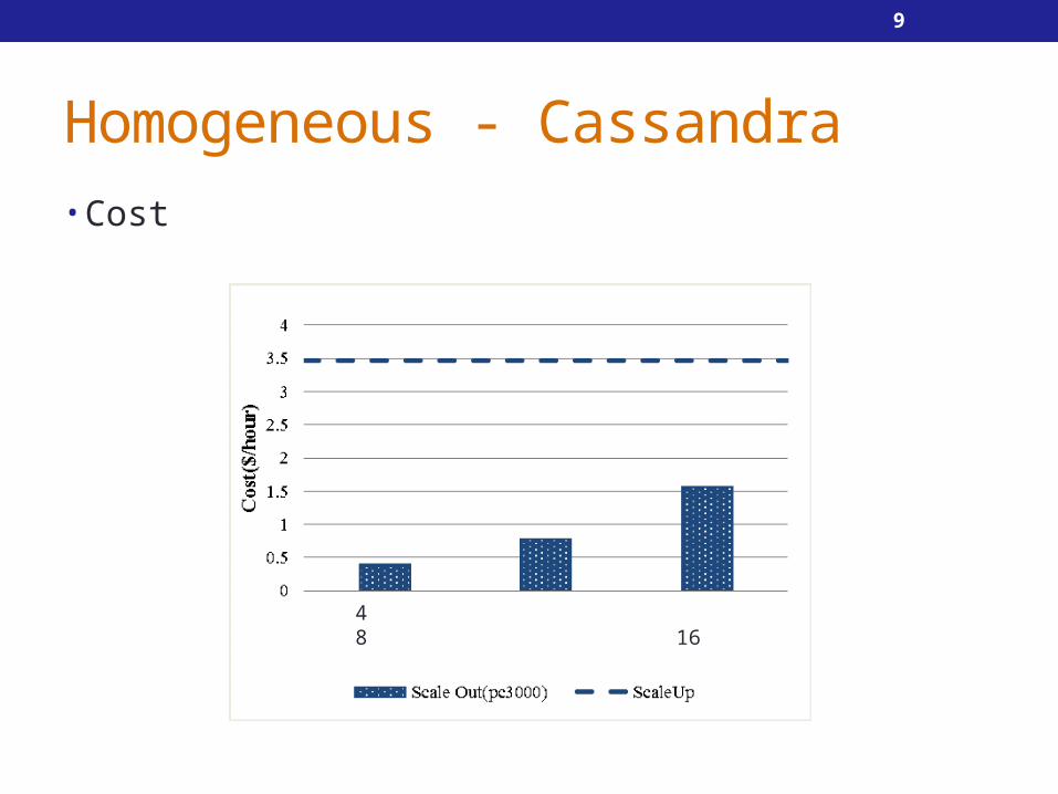
Homogeneous - Cassandra• Cost

4 8 16

10

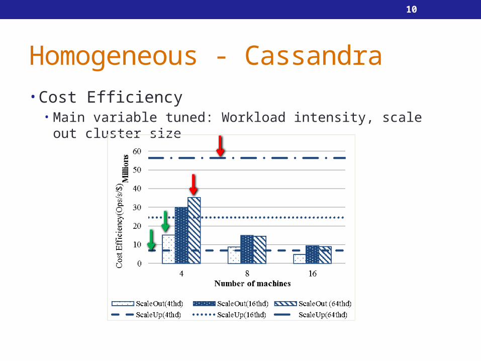
Homogeneous - Cassandra• Cost Efficiency

• Main variable tuned: Workload intensity, scale out cluster size

11

Homogeneous - Cassandra

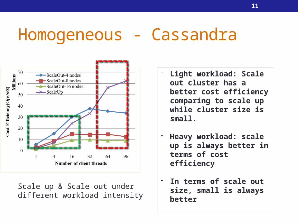
Scale up & Scale out under different workload intensity

- Light workload: Scale out cluster has a better cost efficiency comparing to scale up while cluster size is small.

- Heavy workload: scale up is always better in terms of cost efficiency

- In terms of scale out size, small is always better

12

Homogeneous - Cassandra

Budget-constrained Min throughput requirement

Light workloads Scale out withsmall number of nodes

If throughput low Scale outElse Scale up

Heavy workloads If $ constraint low Scale out is only option Else Scale up

Scale up

13

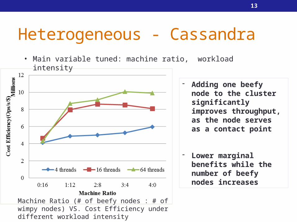
Heterogeneous - Cassandra

Machine Ratio (# of beefy nodes : # of wimpy nodes) VS. Cost Efficiency under different workload intensity

• Main variable tuned: machine ratio, workload intensity

- Adding one beefy node to the cluster significantly improves throughput, as the node serves as a contact point

- Lower marginal benefits while the number of beefy nodes increases

14

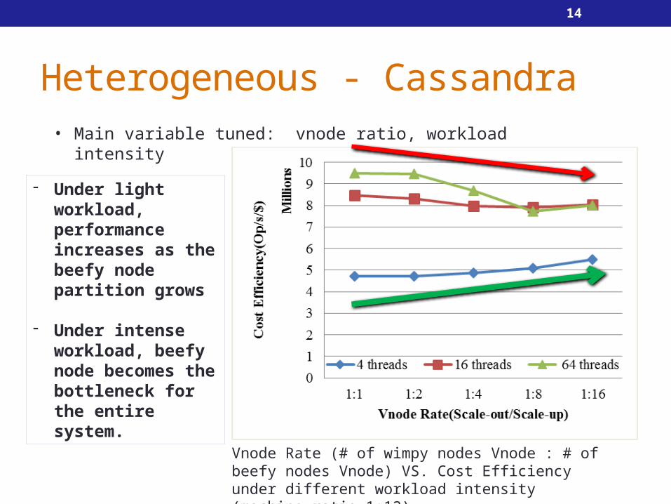
Heterogeneous - Cassandra

Vnode Rate (# of wimpy nodes Vnode : # of beefy nodes Vnode) VS. Cost Efficiency under different workload intensity (machine ratio 1:12)

• Main variable tuned: vnode ratio, workload intensity

- Under light workload, performance increases as the beefy node partition grows

- Under intense workload, beefy node becomes the bottleneck for the entire system.

15

Scale up VS. Scale out - GraphLab

• GraphLab Metrics• Throughput: MB per sec• Cost: Total $ for a workload

• since batch processing system• Normalized metric

• Cost efficiency = Throughput / Cost

16

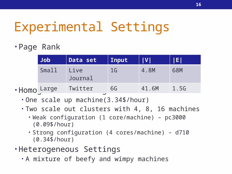
Experimental Settings• Page Rank

• Homogeneous Settings• One scale up machine(3.34$/hour)• Two scale out clusters with 4, 8, 16 machines

• Weak configuration (1 core/machine) – pc3000 (0.09$/hour)• Strong configuration (4 cores/machine) – d710 (0.34$/hour)

• Heterogeneous Settings• A mixture of beefy and wimpy machines

Job Data set Input |V| |E|

Small Live Journal 1G 4.8M 68M

Large Twitter 6G 41.6M 1.5G

17

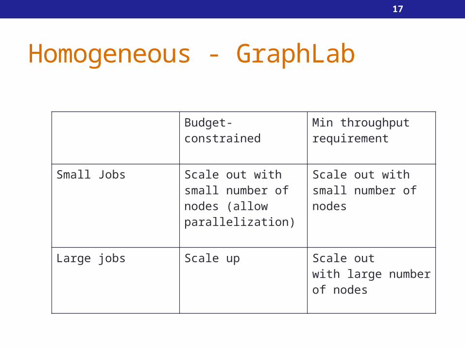
Homogeneous - GraphLab

Budget-constrained Min throughput requirement

Small Jobs Scale out withsmall number of nodes (allow parallelization)

Scale out withsmall number of nodes

Large jobs Scale up Scale outwith large number of nodes

18

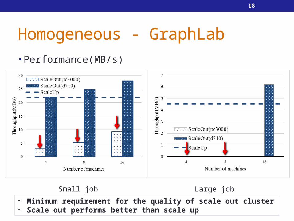
Homogeneous - GraphLab• Performance(MB/s)

Small job Large job

- Minimum requirement for the quality of scale out cluster- Scale out performs better than scale up

19

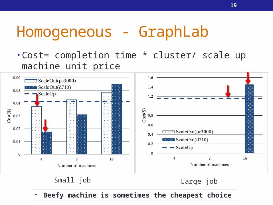
Homogeneous - GraphLab• Cost= completion time * cluster/ scale up machine unit

price

Small job Large job

- Beefy machine is sometimes the cheapest choice

20

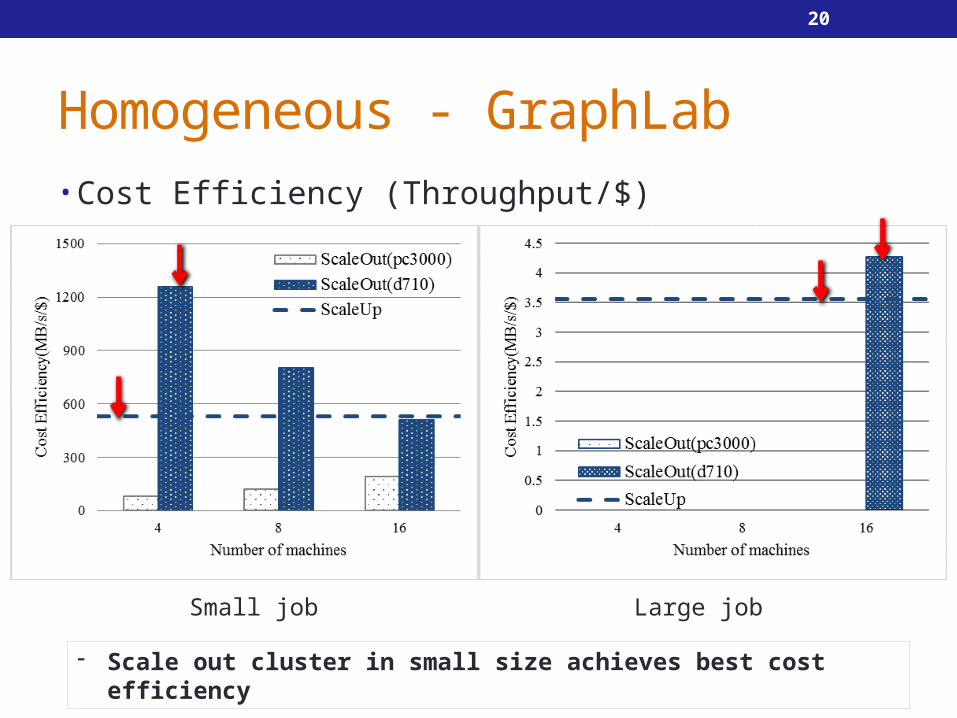
Homogeneous - GraphLab• Cost Efficiency (Throughput/$)

Small job Large job

- Scale out cluster in small size achieves best cost efficiency

21

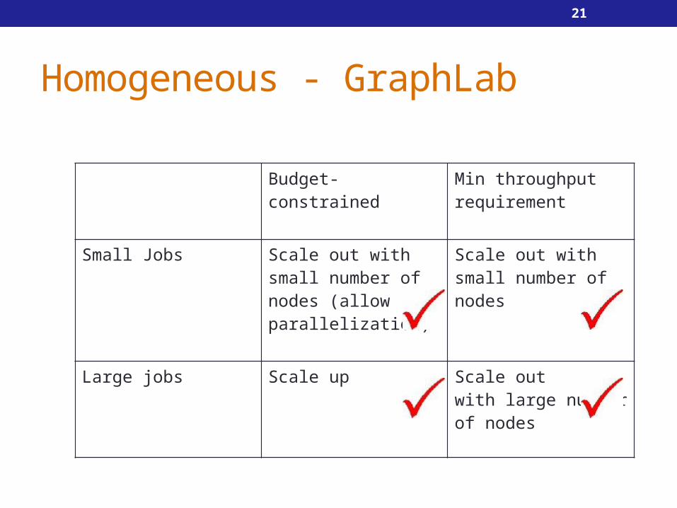
Homogeneous - GraphLab

Budget-constrained Min throughput requirement

Small Jobs Scale out withsmall number of nodes (allow parallelization)

Scale out withsmall number of nodes

Large jobs Scale up Scale outwith large number of nodes

22

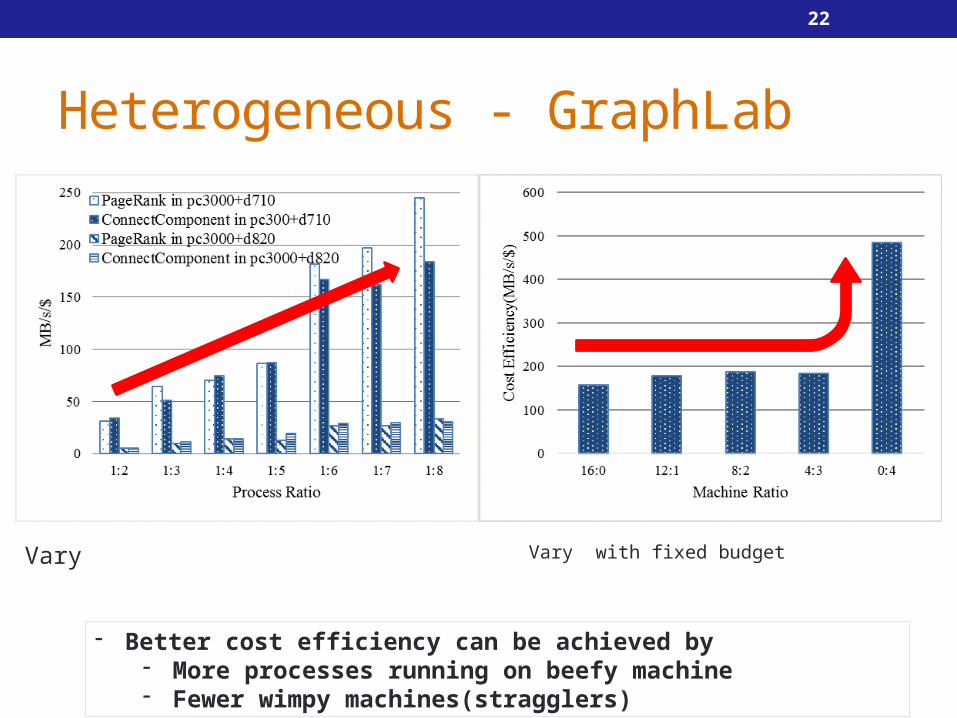
Heterogeneous - GraphLab

Vary Vary with fixed budget

- Better cost efficiency can be achieved by- More processes running on beefy machine- Fewer wimpy machines(stragglers)

23

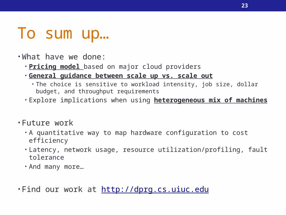
To sum up…• What have we done:

• Pricing model based on major cloud providers• General guidance between scale up vs. scale out

• The choice is sensitive to workload intensity, job size, dollar budget, and throughput requirements

• Explore implications when using heterogeneous mix of machines

• Future work• A quantitative way to map hardware configuration to cost efficiency• Latency, network usage, resource utilization/profiling, fault

tolerance• And many more…

• Find our work at http://dprg.cs.uiuc.edu

24

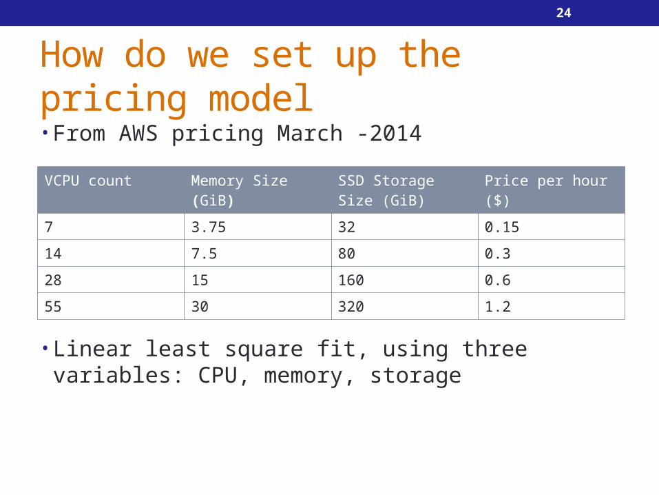
How do we set up the pricing model• From AWS pricing March -2014

• Linear least square fit, using three variables: CPU, memory, storage

VCPU count Memory Size (GiB) SSD Storage Size (GiB)

Price per hour ($)

7 3.75 32 0.15

14 7.5 80 0.3

28 15 160 0.6

55 30 320 1.2

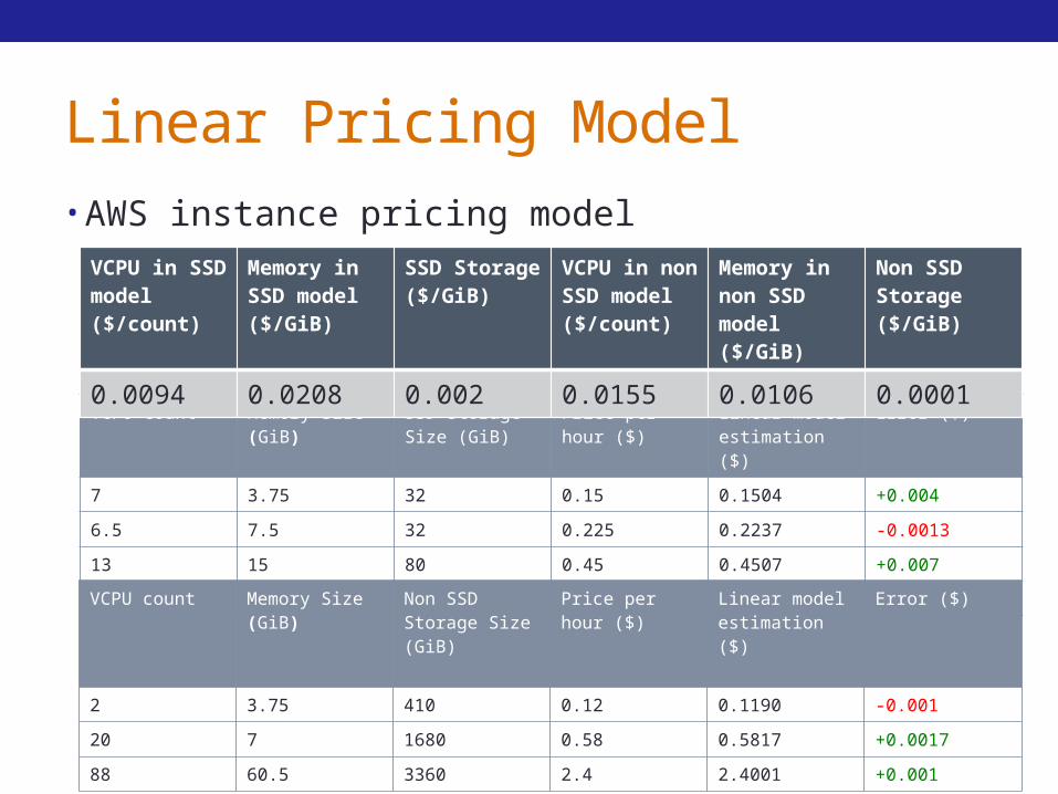
Linear Pricing Model• AWS instance pricing model

VCPU count Memory Size (GiB)

SSD Storage Size (GiB)

Price per hour ($)

Linear model estimation ($)

Error ($)

7 3.75 32 0.15 0.1504 +0.004

6.5 7.5 32 0.225 0.2237 -0.0013

13 15 80 0.45 0.4507 +0.007

108 60 640 2.4 2.3940 -0.006

VCPU count Memory Size (GiB)

Non SSD Storage Size (GiB)

Price per hour ($)

Linear model estimation ($)

Error ($)

2 3.75 410 0.12 0.1190 -0.001

20 7 1680 0.58 0.5817 +0.0017

88 60.5 3360 2.4 2.4001 +0.001

VCPU in SSD model ($/count)

Memory in SSD model ($/GiB)

SSD Storage ($/GiB)

VCPU in non SSD model ($/count)

Memory in non SSD model ($/GiB)

Non SSD Storage ($/GiB)

0.0094 0.0208 0.002 0.0155 0.0106 0.0001

26

Contribution of our work• Setting up pricing model• Storage (Cassandra)

• Homogeneous: Scale out using a small cluster only when there is a dollar budget cap and low throughput requirements, scale up in any other cases.

• Heterogeneous: beefy node is preferable, assigning larger data partition to the beefy node without overwhelms it.

• Graph processing• GraphLab performance and cost efficiency under homogeneous

environment• GraphLab performance and cost efficiency under heterogeneous

environment