SCALE - University of Michigandanbrown/papers/scale_chapter.pdf · CHAPTER FOUR SCALE ... how to automate scale change and simultaneously represent data at ... graphic models that

CHAPTER FOUR

SCALE

Nina Lam, Louisiana State University David Catts, U.S. Geological Survey

Dale Quattrochi, NASA–Global Hydrology and Climate Center Daniel Brown, University of Michigan

Robert McMaster, University of Minnesota

4.1 INTRODUCTION This research priority calls attention to the multidisciplinary issues related to scale in the spatial as well as spatiotemporal domains. The objective of this chapter is to clarify and assess what scale and scale effects are, and through recognizing the fundamental existence of scale effects, determine how one can realistically approach and mitigate them. Primary issues therefore center on gaining a better understanding of how to effectively and efficiently measure and charac-terize scale; how to use scale information in judging the fitness of data for a particular use; how to automate scale change and simultaneously represent data at multiple scales; how scale and change in scale affect information content, analysis, and conclusions about patterns and processes.

The issue of scale is not new, nor is it a concern restricted to geographic information scientists. Scale variations have long been known to constrain the detail with which information can be observed, represented, analyzed, and communicated. Changing the scale of data without first understanding the effects of such action can result in the representation of processes or patterns that are different from those intended. For example, research has shown that reducing the resolution of a raster land cover map (going to larger cells) can increase the dominance of the contiguous classes, but decrease the amount of small and scattered classes (like wetlands in some locations) in the representation (Turner et al., 1989). The spatial scaling problem presents one of the major impediments, both conceptually and methodologically, to advancing all sciences that use geographic information. Likewise, temporal scaling, a separate but related issue,

2 The Research Agenda of Consortium for Geographic Information Science

is not well understood and thus difficult to formalize. In an information era, massive amount of geographic data are collected from various sources, often at different scales. Before these data can be integrated for problem solving, funda-mental issues must be addressed.

Recent work on the scaling behavior of various phenomena and processes (e.g., research in global change, ecological modeling, and environmental health) has shown that many processes do not scale linearly. The implication is that in order to characterize a pattern or process at a scale other than the scale of observation, some knowledge of how that pattern or process changes with scale is needed so that the scaling process can be adjusted accordingly. Attempts to describe scaling behavior by fractals or self-affine models, which mathematically relate complexity and scale, have been made. However, because the fractal model and its realizations have been interpreted and used differently by different researchers (e.g., strict versus statistical self-similarity), the results from applying the fractal model are inconsistent and the approach receives mixed review (Lam and De Cola, 1993). Multifractals have shown some promise for characterizing the scaling behavior of some phenomena, but it is more likely that fractals will offer only a partial model (Pecknold, et al., 1997). Alternative models such as the multi-resolution based wavelet approach are needed to understand the impacts that changes in scale have on the information content of databases (e.g., Mallat, 1989). Examining the sensitivity of processes and analytical models to scale will help scientists validate hypotheses and reduce model uncertainties, which in turn will improve geographic theory-building.

Despite a longstanding recognition of the implications of scale on geo-graphic inference and decision making, many questions remain unanswered. The transition from analog (e.g., maps) to digital representations of geographic infor-mation forces users of those data to formally deal with these conceptual, technical, and analytical questions in new ways. It is easy to demonstrate by isolated examples that scale poses constraints and limitations on geographic information, spatial analysis, and models of the real world. The challenge is to articulate the condi-tions under which scale-imposed constraints are systematic and to develop geo-graphic models that compensate or standardize scale-based variation. Mishandling or misunderstanding scale can bias inference and reasoning and ultimately affect decision-making processes. New types of analyses, for example the Geographical Analysis Machine (GAM) proposed by Openshaw et al. (1987) and the spatial Scan statistic by Kulldorff (1997), offer methods that explore scale effects more easily and may be less sensitive to scale than traditional quantitative techniques.

The widespread adoption of geographic information science has made the scale problem more acute and the need to develop solutions to cope with the scale effects more pressing. Geographic information systems (GISs) facilitate data inte-gration regardless of scale differences. Common problems are when we try to use coarse aggregate data (e.g., statewide or countywide data) and to compare those data with less coarse or disaggregate data (e.g. data defined by census tract or by individual survey). The capability to process and present geographic information “up” and “down” from local, regional, to global scales has been advocated as a

Scale 3

solution to understanding the global systems of both natural (e.g., global climate change) and societal (e.g., global economy) processes and the relationships between the two. Fundamental scale questions will benefit from coordinated research efforts among geographic information scientists with various interests and domain experts. Information systems of the future can sensitize users to the implications of scale dependence and provide scale management tools once we develop useful models of scale behavior, an improved understanding of the effects of scale, novel methods for describing the scale of data, and intelligent automation methods for changing scale.

In the following, we first clarify the scope of scale by describing its various definitions and meanings used in related fields. A widespread adoption of stan-dardized terminology is necessary for better communications between researchers within and among various fields and disciplines. We will then illustrate some concrete examples of how scale might affect our understanding of geographical pheno-mena and hence our decision making in a number of application areas, including cartography, environmental policy, global land-cover change, and environmental health. Emphasis is placed on what researchers/decision makers have done to cope with the scale problem. This is followed by a brief synopsis of what is left to be done and the research challenge lies ahead.

4.2 MEANING AND SCOPE OF THE SCALE ISSUE The term “scale” has been used in different manners under different contexts, making the comparison and communication among researchers and research results across subfields and disciplines more difficult. Typically, when an issue of scale is involved in a scientific paper or study, an explanation of the term is often provided at the beginning of the paper to avoid confusion in subsequent reading. While it may be counterproductive to uncover exhaustively the various meanings of sale, it is important to clarify what we mean and what the scope is when we are referring to the issue of scale in geographic information science.

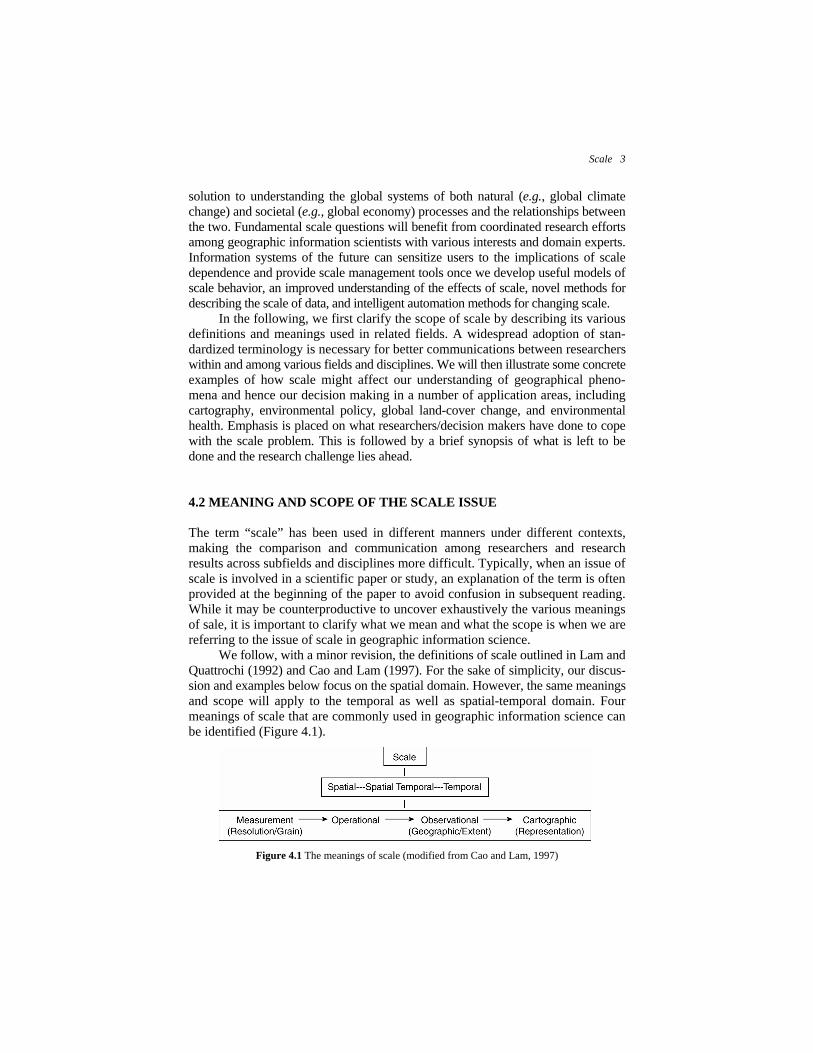
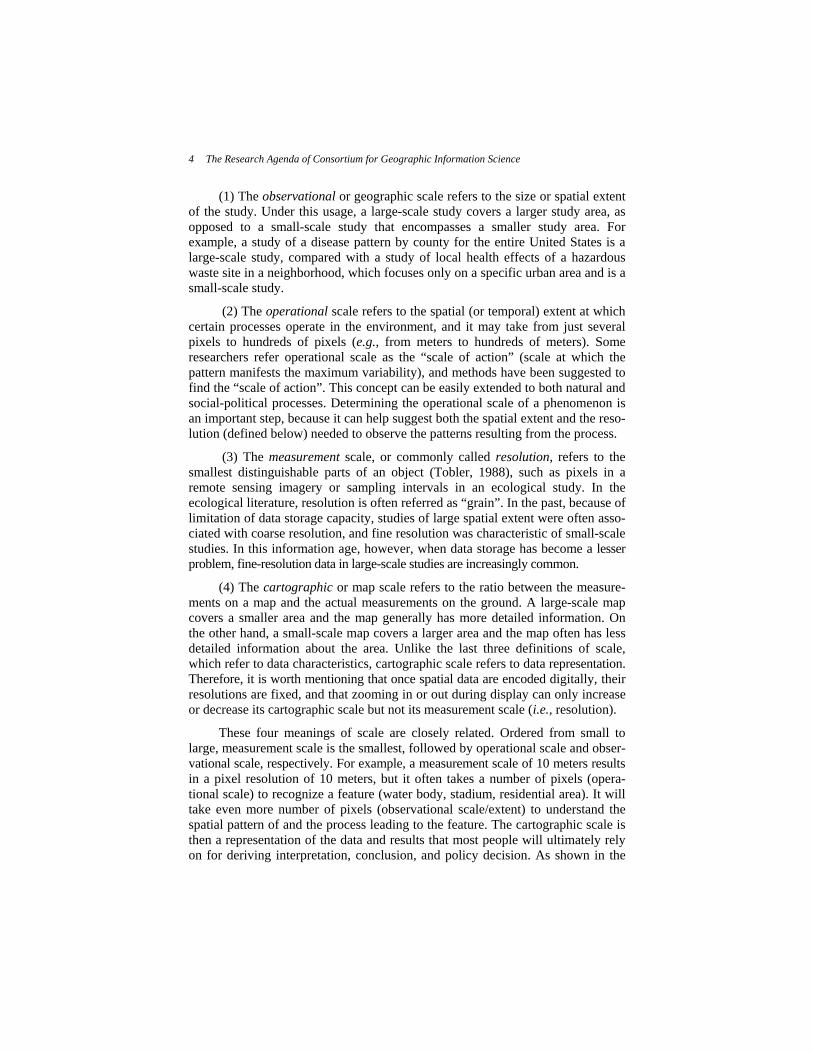
We follow, with a minor revision, the definitions of scale outlined in Lam and Quattrochi (1992) and Cao and Lam (1997). For the sake of simplicity, our discus-sion and examples below focus on the spatial domain. However, the same meanings and scope will apply to the temporal as well as spatial-temporal domain. Four meanings of scale that are commonly used in geographic information science can be identified (Figure 4.1).

Figure 4.1 The meanings of scale (modified from Cao and Lam, 1997)


(1) The observational or geographic scale refers to the size or spatial extent of the study. Under this usage, a large-scale study covers a larger study area, as opposed to a small-scale study that encompasses a smaller study area. For example, a study of a disease pattern by county for the entire United States is a large-scale study, compared with a study of local health effects of a hazardous waste site in a neighborhood, which focuses only on a specific urban area and is a small-scale study.

(2) The operational scale refers to the spatial (or temporal) extent at which certain processes operate in the environment, and it may take from just several pixels to hundreds of pixels (e.g., from meters to hundreds of meters). Some researchers refer operational scale as the “scale of action” (scale at which the pattern manifests the maximum variability), and methods have been suggested to find the “scale of action”. This concept can be easily extended to both natural and social-political processes. Determining the operational scale of a phenomenon is an important step, because it can help suggest both the spatial extent and the reso-lution (defined below) needed to observe the patterns resulting from the process.

(3) The measurement scale, or commonly called resolution, refers to the smallest distinguishable parts of an object (Tobler, 1988), such as pixels in a remote sensing imagery or sampling intervals in an ecological study. In the ecological literature, resolution is often referred as “grain”. In the past, because of limitation of data storage capacity, studies of large spatial extent were often asso-ciated with coarse resolution, and fine resolution was characteristic of small-scale studies. In this information age, however, when data storage has become a lesser problem, fine-resolution data in large-scale studies are increasingly common.

(4) The cartographic or map scale refers to the ratio between the measure-ments on a map and the actual measurements on the ground. A large-scale map covers a smaller area and the map generally has more detailed information. On the other hand, a small-scale map covers a larger area and the map often has less detailed information about the area. Unlike the last three definitions of scale, which refer to data characteristics, cartographic scale refers to data representation. Therefore, it is worth mentioning that once spatial data are encoded digitally, their resolutions are fixed, and that zooming in or out during display can only increase or decrease its cartographic scale but not its measurement scale (i.e., resolution).

These four meanings of scale are closely related. Ordered from small to large, measurement scale is the smallest, followed by operational scale and obser-vational scale, respectively. For example, a measurement scale of 10 meters results in a pixel resolution of 10 meters, but it often takes a number of pixels (opera-tional scale) to recognize a feature (water body, stadium, residential area). It will take even more number of pixels (observational scale/extent) to understand the spatial pattern of and the process leading to the feature. The cartographic scale is then a representation of the data and results that most people will ultimately rely on for deriving interpretation, conclusion, and policy decision. As shown in the

Scale 5

next section, decisions on cartographic scale and generalization are very much based on the data characteristics themselves, such as spatial and thematic resolution.

In defining the meanings and scope of scale, it is important to note not only that consistent terminology must be developed, but also researchers must adopt them widely. The “science of scales” will not progress until some fundamental building blocks, in this case lexical meanings of scale, have been laid out and agreed upon. 4.3 SCALE IN SELECTED APPLICATION AREAS 4.3.1 Cartography and Cartographic Generalization There are five scale-related ingredients that affect the decisions made in carto-graphic design and presentation: cartographic scale, measurement scale (resolu-tion), data model (representation), phenomena, and temporal scale. Each of these elements has unique characteristics and graphic resolutions, and all of these elements interact to challenge the graphic abstraction in cartography. 4.3.1.1 Cartographic Scale Map scale is often neglected in many day-to-day maps. We encounter maps each day and unfortunately many of these do not have any reference of map scale. In some cases, the scale is purposefully distorted to promote a particular point of view (Monmonier, 1991), and the reader more often presumes the consistency of scale. The effective use of perspective views in cartography is an example that complicates the conventional design notion of adhering to uniform map scales.

The overall purpose of selecting a map scale is to provide map integrity, either by specifying the “exact proportions” for measurement or by maintaining relative geospatial relationships of geophysical features. Other cartographic elements of integrity are the use of an appropriate projection and datum, and providing reference information and some notations about the date and source of the reference materials used in the map design. By providing a “coverage diagram” or “source statement”, the map designer can exactly specify the source material used in various areas of the map compilation.

The determining factors in selecting an appropriate map scale are geo-graphical extent and final map size (Robinson, et al., 1995). The output media available may also predetermine the scale of a map. By selecting one of the various digital output options available to cartography, we are no longer restricted by the artistic possibilities of the paper and pen but by the size and resolution of the digital media. Paper printers vary in resolution generally from 72 dots per inch (DPI) to 1200 DPI. Film recorders approach 1,200–2,400 DPI in resolution. The effective design of Internet maps is a more difficult challenge as screen reso-lutions and color qualities vary. In each design case, the resolutions and colors of


the targeted media place technological restrictions on the size, colors, and overall quality of the map. These graphic restrictions place limits on what scale and content can be presented effectively.

There are various examples that illustrate how paper size or ease of measure-ment conventions predetermines the map scale. For example, the USDA Forest Service uses a scale of 1:126,720 for general reference maps of National Forests, and this proportion results in one inch of map distance equaling exactly 2 miles. The U.S. Geological Survey (USGS) produces over 25,000 1:24,000-scale maps of the United States, and all but a selected number are composed and revised at this standard series scale of 1 inch equaling 2,000 feet. In each case, the conven-tions of using a standardized map scale alter the symbol density and our percep-tions of a feature’s importance (Figure 4.2).

Figure 4.2 Standardized scale series complicate the design for sparse and congested

symbolization. Shown here are comparative graphic areas of feature content for a fixed scale map series (USGS 1:24,000 Freemason Island, LA (left) and Central Park, NY.)

4.3.1.2 Measurement Scale (Resolution) It is generally accepted that data compilation should occur at a finer resolution than the final map. The detail of compiled features is then selected, prioritized, and generalized as the map is compiled and assembled. Feature selection and con-tent generalization are integrated into the cartographic process, and the term “cartographic license” is used to denote the composition and balancing of various cartographic components such as content, color, and symbols of the map.

The integration of geographic information systems throughout our society has provided the means for all of us to be portrayers of geospatial data. This ability to select and integrate data of disparate resolution and source expands the meaning of “cartographic license” beyond one of strictly map composition. The data sources used in the design may vary in map scale, source, content density, and resolution. It is the map design process that strives to balance the variety of these data characteristics in a meaningful and truthful way. GIS and the associated technologies allow all of us to “slam” data sets together to produce a result that

nlam

importance (Figure

Scale 7

may appear truthful or promotes integrity. The technological abilities of GIS underscore the warning of mismatched scales, as data of varying scales can be merged, warped, and conflated to present an intended message.

The determining factor in cartographic design is, “what is the purpose of the map?” From a content perspective, unimproved dirt roads may seem unimportant for a regional transportation map, but these access routes are extremely important at any scale when the map purpose is to show the potential impact of these access routes on undeveloped or roadless areas. In a hydrologic example, removing the lowest Strahler stream order class might reduce the graphic density of the drainage pattern. In a realistic situation, the subsurface geology of the area might produce perennial streams on one side of a ridge that flow year round, and these isolated streams become an important water source to be represented throughout a wider range of map scale. The geophysical relationships between data themes and within the entire context of the map’s purpose need to be established for better map design.

4.3.1.3 Scale of the Data Model (Representation) The integrity of the data resolution, and its scaleable characteristics, can be rede-fined by the data model used in storing, processing, and representing features. For example, the exact ground coordinate values can be truncated further by GIS systems that use disparate data precision to store the data internally; therefore the GIS data model and not the data itself further redefine the resolution of the data.

Changing scales of the data representation requires cartographic generaliza-tion. The challenge of the map design is to balance the map content to what is the threshold of sufficient information. If there is not enough space for the most important information, we find ways to redesign and repackage the map symbol-ogy, or we change the size of the design parameters. In representing distinct occurrences of phenomena across various scales, we use “representative patterns” of symbols to define the collective occurrence.

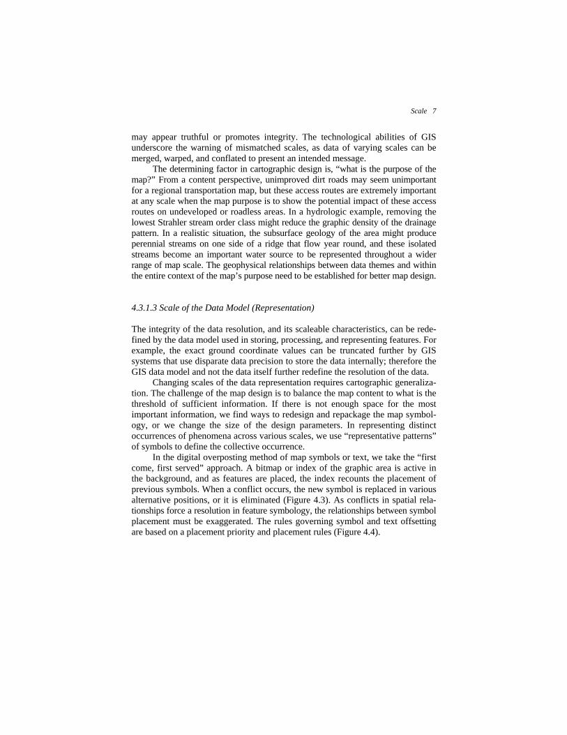
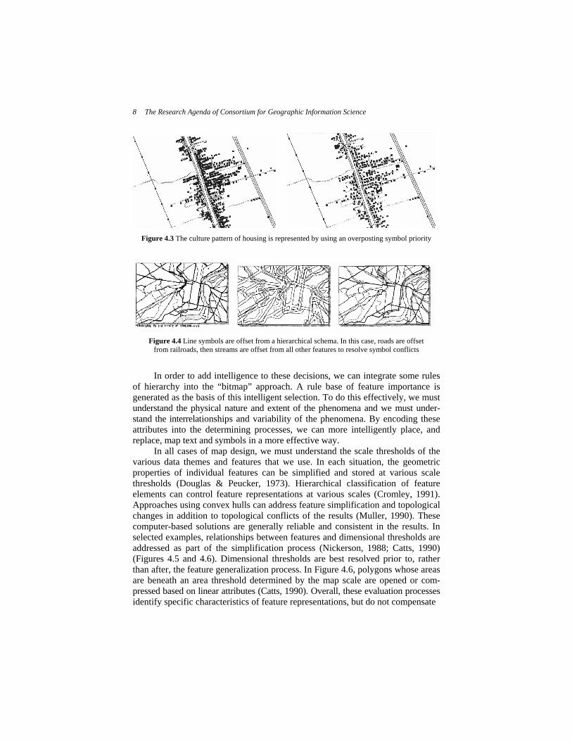
In the digital overposting method of map symbols or text, we take the “first come, first served” approach. A bitmap or index of the graphic area is active in the background, and as features are placed, the index recounts the placement of previous symbols. When a conflict occurs, the new symbol is replaced in various alternative positions, or it is eliminated (Figure 4.3). As conflicts in spatial rela-tionships force a resolution in feature symbology, the relationships between symbol placement must be exaggerated. The rules governing symbol and text offsetting are based on a placement priority and placement rules (Figure 4.4).


Figure 4.3 The culture pattern of housing is represented by using an overposting symbol priority

Figure 4.4 Line symbols are offset from a hierarchical schema. In this case, roads are offset

from railroads, then streams are offset from all other features to resolve symbol conflicts

In order to add intelligence to these decisions, we can integrate some rules of hierarchy into the “bitmap” approach. A rule base of feature importance is generated as the basis of this intelligent selection. To do this effectively, we must understand the physical nature and extent of the phenomena and we must under-stand the interrelationships and variability of the phenomena. By encoding these attributes into the determining processes, we can more intelligently place, and replace, map text and symbols in a more effective way.

In all cases of map design, we must understand the scale thresholds of the various data themes and features that we use. In each situation, the geometric properties of individual features can be simplified and stored at various scale thresholds (Douglas & Peucker, 1973). Hierarchical classification of feature elements can control feature representations at various scales (Cromley, 1991). Approaches using convex hulls can address feature simplification and topological changes in addition to topological conflicts of the results (Muller, 1990). These computer-based solutions are generally reliable and consistent in the results. In selected examples, relationships between features and dimensional thresholds are addressed as part of the simplification process (Nickerson, 1988; Catts, 1990) (Figures 4.5 and 4.6). Dimensional thresholds are best resolved prior to, rather than after, the feature generalization process. In Figure 4.6, polygons whose areas are beneath an area threshold determined by the map scale are opened or com-pressed based on linear attributes (Catts, 1990). Overall, these evaluation processes identify specific characteristics of feature representations, but do not compensate

Scale 9

Figure 4.5 The dimensional characteristics and transitions of area hydrography

are resolved by using a minimum threshold (from Nickerson, 1988)

Figure 4.6 Small area hydrographic features are eliminated, and the linear network is resolved to maintain topological feature relationships before feature simplification (from Catts, 1990)

for variety and interrelationships for determining dimensional thresholds of features than govern our asystematic and artistic decisions in map composition.

In order to effectively portray map content across scales, the two schools of thought are that map features can be represented as distinct and static repre-sentations of scale-specific content (example: scale series of 1:24,000; 1:100,000, 1:250,000), or that spatial features can be intelligently analyzed to generate the selection interactively in the generalization process. In selected examples, these approaches are integrated into a unique process of scaleable representations and


functions within the data structure itself (Buttenfield, 1984), such as the Geographic Data Files (GDF) developed in Europe (Figure 4.7).

Figure 4.7 Geographic data files contain multiple representations of features

for use at various scale thresholds (ERTICO, 1997)

As part of Project 615, the Forest Service is developing feature generali-

zation techniques that allow for multiscale representations of its geographic data (Rodriguez, 1998). This activity addresses a comprehensive feature and symbol generalization for both the Forest Service 1:24,000 and 1:126,720 scaled series from a single geographic database. The complexity of addressing both feature simplification and symbol resolution will provide an integrated solution and knowledge base for developing multiscale representations from a single data source.

4.3.1.4 Scale and Dimensional Thresholds of Phenomena What the feature scaling process presents to cartographic design are dimensional changes of the symbolized features. A simple example is that a cased-road might become a single line as the scale decreases, but clusters of polygons may interact in various ways. A collection of swampy areas may be distinctly mapped at a large scale, and as scale decreases these individual polygon areas might combine to become a “swampy area” in a larger sense (Figure 4.8). Eventually, these fea-tures may shift to another dimensional representation or disappear from the map.

Figure 4.8 As the scale decreases, the symbolization of swampy areas shift in dimension

from unique areas, to selectively aggregate areas, to point symbols in a pattern

nlam

1997)

Scale 11

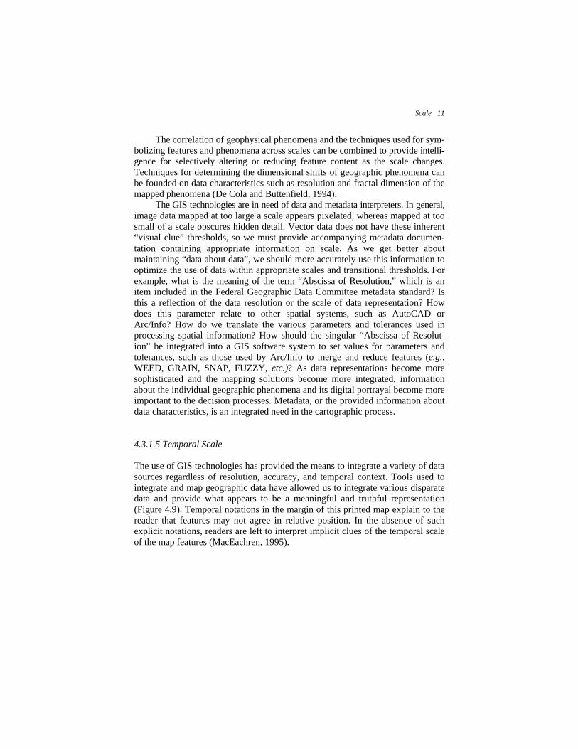
The correlation of geophysical phenomena and the techniques used for sym-bolizing features and phenomena across scales can be combined to provide intelli-gence for selectively altering or reducing feature content as the scale changes. Techniques for determining the dimensional shifts of geographic phenomena can be founded on data characteristics such as resolution and fractal dimension of the mapped phenomena (De Cola and Buttenfield, 1994).

The GIS technologies are in need of data and metadata interpreters. In general, image data mapped at too large a scale appears pixelated, whereas mapped at too small of a scale obscures hidden detail. Vector data does not have these inherent “visual clue” thresholds, so we must provide accompanying metadata documen-tation containing appropriate information on scale. As we get better about maintaining “data about data”, we should more accurately use this information to optimize the use of data within appropriate scales and transitional thresholds. For example, what is the meaning of the term “Abscissa of Resolution,” which is an item included in the Federal Geographic Data Committee metadata standard? Is this a reflection of the data resolution or the scale of data representation? How does this parameter relate to other spatial systems, such as AutoCAD or Arc/Info? How do we translate the various parameters and tolerances used in processing spatial information? How should the singular “Abscissa of Resolut-ion” be integrated into a GIS software system to set values for parameters and tolerances, such as those used by Arc/Info to merge and reduce features (e.g., WEED, GRAIN, SNAP, FUZZY, etc.)? As data representations become more sophisticated and the mapping solutions become more integrated, information about the individual geographic phenomena and its digital portrayal become more important to the decision processes. Metadata, or the provided information about data characteristics, is an integrated need in the cartographic process.

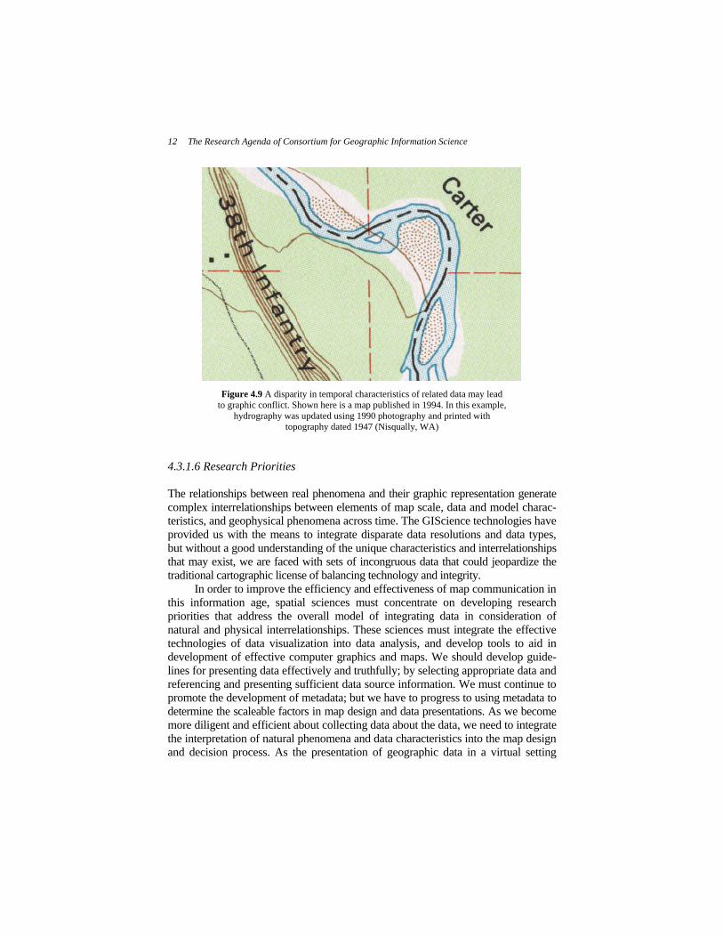
4.3.1.5 Temporal Scale The use of GIS technologies has provided the means to integrate a variety of data sources regardless of resolution, accuracy, and temporal context. Tools used to integrate and map geographic data have allowed us to integrate various disparate data and provide what appears to be a meaningful and truthful representation (Figure 4.9). Temporal notations in the margin of this printed map explain to the reader that features may not agree in relative position. In the absence of such explicit notations, readers are left to interpret implicit clues of the temporal scale of the map features (MacEachren, 1995).


Figure 4.9 A disparity in temporal characteristics of related data may lead

to graphic conflict. Shown here is a map published in 1994. In this example, hydrography was updated using 1990 photography and printed with

topography dated 1947 (Nisqually, WA) 4.3.1.6 Research Priorities The relationships between real phenomena and their graphic representation generate complex interrelationships between elements of map scale, data and model charac-teristics, and geophysical phenomena across time. The GIScience technologies have provided us with the means to integrate disparate data resolutions and data types, but without a good understanding of the unique characteristics and interrelationships that may exist, we are faced with sets of incongruous data that could jeopardize the traditional cartographic license of balancing technology and integrity.

In order to improve the efficiency and effectiveness of map communication in this information age, spatial sciences must concentrate on developing research priorities that address the overall model of integrating data in consideration of natural and physical interrelationships. These sciences must integrate the effective technologies of data visualization into data analysis, and develop tools to aid in development of effective computer graphics and maps. We should develop guide-lines for presenting data effectively and truthfully; by selecting appropriate data and referencing and presenting sufficient data source information. We must continue to promote the development of metadata; but we have to progress to using metadata to determine the scaleable factors in map design and data presentations. As we become more diligent and efficient about collecting data about the data, we need to integrate the interpretation of natural phenomena and data characteristics into the map design and decision process. As the presentation of geographic data in a virtual setting

Scale 13

become more sophisticated, we need to develop visual clues to the varieties of scale and temporal characteristics of the data. We should develop knowledge of the dimensional thresholds of natural phenomena and the graphic abstractions with which they are represented. Multiple representations of features across scale and symbology thresholds should be promoted. Overall, we must promote the integrity of geographic data visualization in the variety of new cartographic technologies and products that are available to society.

4.3.2 Environmental Policy and Decision Making The Earth’s surface environmental properties are characterized in a manner that ultimately, gives the appearance of spatial pattern. Because of the structure of these environmental properties, however, the scale (geographical and operational) at which these properties can be identified, observed, or measured is limited by the resolution of the measurement technology. One primary aim in geographical analysis is to identify and describe the pattern or scale of variation in spatial phenomena at the level of resolution of interest. This level of resolution can vary immensely depending upon what the objectives are for observation or measure-ment, as well as what the overall characteristics are of the spatial object or objects under study (i.e., the operational scale). For example, in analyzing an environ-mental property such as soils, the data resolution (i.e., measurement scale) can range from a soil core sample, a soil series, a field plot, an agricultural field, a county, state or other municipal boundary, including a country, or even the entire globe. At any of these levels, there is likely to be one or more spatial resolutions at which most of the variation occurs (Oliver, 2001). To detect this spatial variability, the level of observation must relate to the spatial (or even temporal) scale at which most of this variation becomes evident (i.e., operational scale). It is important to note as a caveat, however, that what is observed as pattern or spatially correlated variation at one resolution can appear as “noise” or uncor-related variation at another (Oliver, 2001).

As most environmental properties vary continuously over the Earth’s surface, the areas involved in their studies or analyses are large. Information about such properties is either directly derived, or extrapolated from, smaller areas or sampling locations that are separated by much larger areas. Consequently, specific or detailed information can be sparsely distributed, where there may be relatively large intervening spaces about which nothing is known. This is problematic to users of environmental information because they usually want to know what the properties are like everywhere; i.e., from a generalized per-spective. Thus, there is a need to be able to predict either “real” or “inferred” values of environmental properties at unsampled places, but this is difficult in most cases because of the complex nature of spatial variation (Oliver, 2001).

Despite the seemingly inherent complexity of variation in environmental or landscape properties, such as soil moisture distribution or urban sprawl, one


theoretical tenet of geographical analysis is that the values of a spatial pheno-menon that are in close proximity to one another are usually more similar than those that are further apart; i.e., the Tobler’s Law of geography (Tobler, 1970). This relationship between distance (or proximity) and the characteristics of spatial phenomena provides the association that is required to discern the pattern, arrangement, or orientation of these phenomena. Such information can be used to guide sampling intensity or intervals, and to provide clues about the factors and causal processes of spatial variability. The patterns observed through such spatial analysis or interpretation may also form the basis for suggesting the need for different forms of management of the environment (e.g., process-response attributes, cause-effect interactions, land-cover/land-use impacts). Thus, the nature of the environment poses questions such as:

• At what spatial scale should the properties be studied or investigated? • What kind of sampling scheme for observation should be used? • How many samples should be taken? • What sampling interval should be used? • How should values be predicted or inferred at intervening places?

As a result of the wide range of spatial scales (extent and resolution) over which environmental properties can vary, there is an obvious need to consider what the level of scale of interest is at the start of an investigation. Moreover, the detection of spatial variation in environmental phenomena requires adequate sam-pling that is representative, as well as the identification of an appropriate method of estimation or prediction through spatial analysis methodology given the objec-tives of the investigation.

Consideration of scale (geographic extent and operational scale), spatial varia-bility, and resolution can be a confounding and even overbearing problem, however, when attempting to collect, manipulate, analyze, or interpret data for environmental decision-making. This has a number of causes, but perhaps two of the most impor-tant issues are a misunderstanding of the meaning of scale and the explosion of data that are available at different spatial scales (both resolution and extent). As discussed in the beginning of this chapter, there has been much recent discussion of what the definitions of scale and scale concepts are from a mostly quasi-theoretical or aca-demic perspective. However, there has been perhaps a less than compelling focus on the necessity for considering scale implications and their overall importance to environ-mental public policy or environmental decision-making. This is not to say that indivi-duals involved with making sound decisions on a host of environmental issues are not aware of the scale issue and its relation to spatial variability. They have a broad understanding of scale, and in many cases, have a good tacit spatial knowledge. However, as noted by Quattrochi (1993), this tacit perception or understanding of scale causes confusion when inferred or implied spatial concepts are applied with-out due thought to what actually is meant by “scale”. In short, with such things as the very high-resolution remote-sensing data available today, in conjunction with

Scale 15

widespread adoption of geographic information science and technologies, the proverbial “trees” can literally be separated from the “forest” with pinpoint accuracy, without due thought to why this is necessary within the purview of environmental decision-making. The abundance of available spatial data from a plethora of sources with different resolutions, in concert with the increased sophistication of analytical tools (e.g., GISs, image processing software), contributes to the scale problem.

Scale and the interpretation of scale (i.e., what “scale” means and how perceived notions of “scale” are applied by policy and decision-makers or the general public) are central to the measurement of urban functions. Usually, the “functionality” of urban areas is observed at broad geographical scales (as well as coarse resolutions) with a focus on deriving a general rule and functional attributes for the entire urban area. As a result of this coarseness, these definitions or measure-ments of functionality are limited in usefulness for describing or initiating detailed physical or environmental planning policy (Mesev and Longley, 2001). On the contrary, at a very fine scale of analysis (higher resolution and smaller geographical extent), the physical structure of urban attributes allows for the discrimination of discrete characteristics, such as streets and buildings, that provides a spatial perspec-tive of the activity space requirements necessary for urban living. Such information may be of utility for detailed site analysis and planning, but it does not contribute to a broader indication of the overall pattern, arrangement, or orientation of the varia-bility of individual structures or parcels as related to overall urban spatial compo-sition. Consequently, environmental policy or decision-makers could operate at either inappropriate scales or make decisions based on assumptions drawn from using either too coarse or too fine scales. These relationships can be illustrated as follows.

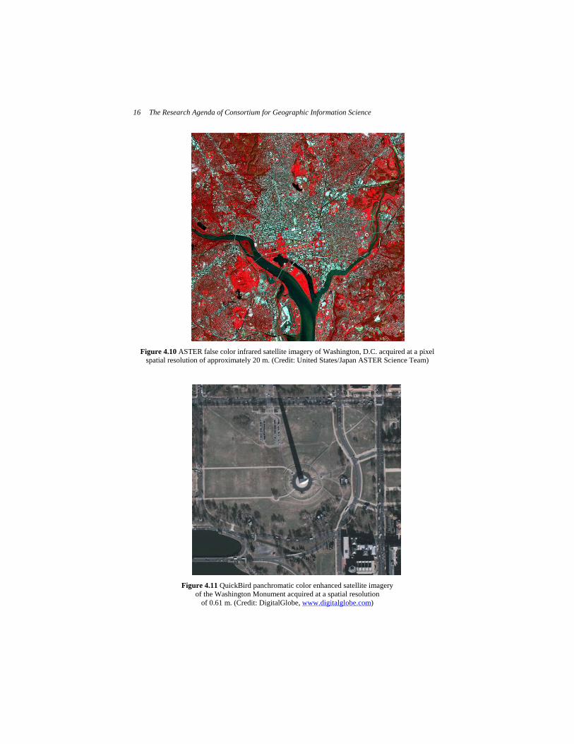
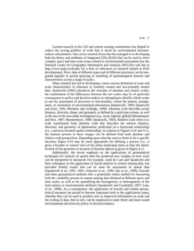
Figure 4.10 is a false color infrared satellite image of Washington, D.C. obtained from the Advanced Spaceborne Thermal Emission and Reflection Radio-meter (ASTER). The ASTER instrument is flown onboard the National Aeronautics and Space Administration (NASA) Terra spacecraft (see the Terra/ASTER web site at http://terra.nasa.gov/About/ASTER/about_aster.html for more information). The area of this image covers 14 km x 13.7 km with a pixel spatial resolution of approximately 20 m. At this spatial resolution, it is possible to discern both coarse and fine patterns or features inherent to the urban structure and fabric of the Washington, D.C. area, such as forest extent, built up areas, residential areas, parks, roadways, streets and clusters of buildings. Figure 4.11 is an image of the Washington Monument acquired by the QuickBird commercial remote sensing satellite (www.digitalglobe.com). This is a natural color image obtained at 0.61 m spatial resolution. It is obvious that the very high spatial resolution of Figure 4.11 is useful, but for a much different set of urban planning or environmental assessment needs than the moderate resolution provided in Figure 4.10. That is, the “trees” (identification or measurement of discrete surfaces) are entirely evident in Figure 4.11, as opposed to the “forest” (identification of general urban patterns of land covers) that is seen from the perspective of Figure 4.10. The urban planner or environmental policy or decision-maker is thus, faced with the quintessential spatial question of which scale to use for analysis of environmental characteristics or processes?


Figure 4.10 ASTER false color infrared satellite imagery of Washington, D.C. acquired at a pixel

spatial resolution of approximately 20 m. (Credit: United States/Japan ASTER Science Team)

Figure 4.11 QuickBird panchromatic color enhanced satellite imagery of the Washington Monument acquired at a spatial resolution

of 0.61 m. (Credit: DigitalGlobe, www.digitalglobe.com)

Scale 17

Current research in the GIS and remote sensing communities has helped to reduce the vexing problem of scale that is faced by environmental decision-makers and planners. One active research focus that has emerged is in developing both the theory and attributes of integrated GISs (IGIS) that can be used to solve complex space and time scale issues related to environmental assessment (see the National Center for Geographic Information and Analysis (NCGIA) web site at http://www.ncgia.ucsb.edu/ for a host of references to research related to IGIS development). Here, data of different types and of different structures can be inte-grated together to permit querying or modeling of spatiotemporal features and characteristics across a range of scales.

Other research has led to developing a more concise definition of scale and scale characteristics in reference to remotely sensed and non-remotely sensed data. Quattrochi (1993) introduces the concepts of absolute and relative scales, the examination of the differences between the two scales may be of particular consequence to policy and decision-makers in attempting to identify which scales to use for assessment of processes or functionality, versus the pattern, arrange-ment, or orientation of environmental phenomena (Quattrochi, 1993; Quattrochi and Goel, 1995; Montello and Golledge, 1998). Absolute scale describes actual distance, direction, shape, and geometry as defined by a grid-type system, as well as the size of the area under investigation (e.g., local, regional, global) (Meentemeyer and Box, 1987; Meentemeyer, 1989; Quattrochi, 1993). Relative scale refers to a scale transformed from absolute scale that describes the relative distance, direction, and geometry of phenomena, predicated on a functional relationship (i.e., a process-oriented spatial relationship). In relation to Figures 4.10 and 4.11, the features present in these images can be defined from both absolute and relative scale perspectives. Depending upon what the need or desire is for a specific decision, Figure 4.10 may be more appropriate for defining a process (i.e., it gives a broader or coarser view of the urban landscape) more so than the identi-fication of the geometry or location of discrete objects as given in Figure 4.11.

Additionally, the recent emphasis on the applications of geostatistical techniques for analysis of spatial data has produced new insights on how scale can be interpreted or measured. For example, work by Lam and Quattrochi and their colleagues on the application of fractal analysis to remote sensing data, has provided fruitful results that can be used for assessment of spatial data (Quattrochi et al., 1997, 2001; Emerson et al., 1999; Qiu et al., 1999). Fractals and other geostatistical methods offer a potentially robust method for measuring both the variability present in remote sensing data obtained at different space and time scales, as well as for quantifying the homogeneity or heterogeneity of the land surface or environmental attributes (Quattrochi and Goodchild, 1997; Lam, et al., 1998). As a consequence, the application of fractals and similar geosta-tistical measures are poised to become important tools in the applications arena, whereby they can be used to produce new or improved information on scale and the scaling of data, that in turn, can be employed to make better and more sound environmental decisions by policy or decision-makers.


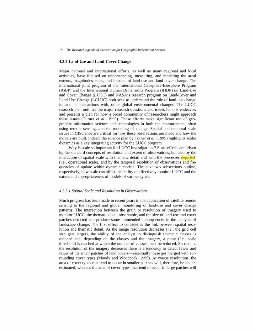
4.3.3 Land-Use and Land-Cover Change Major national and international efforts, as well as many regional and local activities, have focused on understanding, measuring, and modeling the areal extents, magnitudes, rates, and impacts of land-use and land cover change. The international joint program of the International Geosphere-Biosphere Program (IGBP) and the International Human Dimensions Program (IHDP) on Land-Use and Cover Change (LUCC) and NASA’s research program on Land-Cover and Land-Use Change (LCLUC) both seek to understand the role of land-use change in, and its interactions with, other global environmental changes. The LUCC research plan outlines the major research questions and issues for this endeavor, and presents a plan for how a broad community of researchers might approach these issues (Turner et al., 1995). These efforts make significant use of geo-graphic information science and technologies in both the measurement, often using remote sensing, and the modeling of change. Spatial and temporal scale issues in GIScience are critical for how these observations are made and how the models are built. Indeed, the science plan by Turner et al. (1995) highlights scalar dynamics as a key integrating activity for the LUCC program

Why is scale so important for LUCC investigations? Scale effects are driven by the standard concepts of resolution and extent of observations, but also by the interaction of spatial scale with thematic detail and with the processes depicted(i.e., operational scale), and by the temporal resolution of observations and fre-quencies of update within dynamic models. The next two subsections outline, respectively, how scale can affect the ability to effectively monitor LUCC and the nature and appropriateness of models of various types.

4.3.3.1 Spatial Scale and Resolution in Observations Much progress has been made in recent years in the application of satellite remote sensing to the regional and global monitoring of land-use and cover change patterns. The interaction between the grain or resolution of imagery used to monitor LUCC, the thematic detail observable, and the size of land-use and cover patches detected can produce some unintended consequences in the analysis of landscape change. The first effect to consider is the link between spatial reso-lution and thematic detail. As the image resolution decreases (i.e., the grid cell size gets larger), the ability of the analyst to distinguish thematic classes is reduced and, depending on the classes and the imagery, a point (i.e., scale threshold) is reached at which the number of classes must be reduced. Second, as the resolution of the imagery decreases there is a tendency to detect fewer and fewer of the small patches of land covers—essentially these get merged with sur-rounding cover types (Moody and Woodcock, 1995). At coarse resolutions, the area of cover types that tend to occur in smaller patches will, therefore, be under-estimated, whereas the area of cover types that tend to occur in large patches will

nlam

depicted

Scale 19

be overestimated. The interactions are complicated by the influence that differences in the spectral characteristics and definitions of the various cover types have on their detectability, but the general pattern of resolution effects tends to hold.

These scale impacts have affected some very important scientific and policy debates that center on LUCC. A famous example of the effects image resolution can have on LUCC analysis concerns the rate of deforestation in the Brazilian Amazon, which holds about 30 percent of the world’s tropical forests and has critical importance to estimates of both the global carbon budget and rates of biodiversity loss. Early estimates of deforestation between 1978 and 1988, made using the Advanced Very High Resolution Radiometer (AVHRR) meteorological satellite sensor with a resolution of 1 km, were compared with an updated analysis, made using Landsat Multispectral Scanner (MSS) imagery with a resolution of 60 m (Skole and Tucker, 1993). The results indicated that the coarser resolution imagery overestimated the area deforested by about 50 percent. Because models of carbon cycling and estimates of biodiversity loss both require estimates of LUCC rates, attempts to reconcile the global carbon budget and estimate biodiversity loss were affected by these scale and resolution effects.

Studies of urbanization and urban sprawl must contend with complex interactions between the scale of the phenomena, the resolution of the data used to study them, and the definitions of thematic classes represented. The fine-grained nature of the urban fabric reduces the effectiveness of Landsat-class (e.g., resolution of 20–50 m) satellite imagery in studies of urbanization, especially at the fringes of urban areas where most of the change is taking place (though, see the discussion in section 4.3.2 about the relative merits of coarse and fine resolution imagery for urban environments). The thematic classes used in LUCC studies involve land use, land cover, or both. The class “urban” refers to a land use, but it is composed of fine-grained pattern of land covers. A coarse-resolution image (i.e., coarser than the grain of the urban landscape) sees only a mixture of land covers in urban areas and that mixture must be interpreted as a land-use class. The ability to interpret detailed land-use classes is limited by the ability to map land cover mixtures to land use (Cihlar and Jansen, 2001). That ability is affected, in non-linear ways, by resolution.

Although urbanization studies have been supported by satellite remote sensing, other sources of information have been at least as useful. At the most detailed, LUCC studies in urban settings use aerial photography, and now high-resolution satellite imagery, because of the ability to detect individual structures and land-parcel level changes. Aerial photographs are often used in conjunction with detailed cadastral (tax parcel) records in a GIS. Another very important source of spatial information for urbanization studies is derived from censuses of population and housing. These data are usually provided for areas on the grounds that correspond to enumeration districts. In the U.S., enumeration districts take the form of census blocks, which are aggregated to form block groups and census tracts. Some planning-oriented analyses further combine census units into planning districts or traffic analysis zones. The resolution of the data in the case of areally


aggregated data is determined by the level at which the data are summarized. Significant work on the modifiable areal unit problem tells us that attempts to characterize urban land use or urban land-use change using census-type data are affected by the size, shape, and position of the spatial units by which those data are aggregated. Different results (i.e., patterns, rates, and policies) can be obtained using data based on different zoning systems.

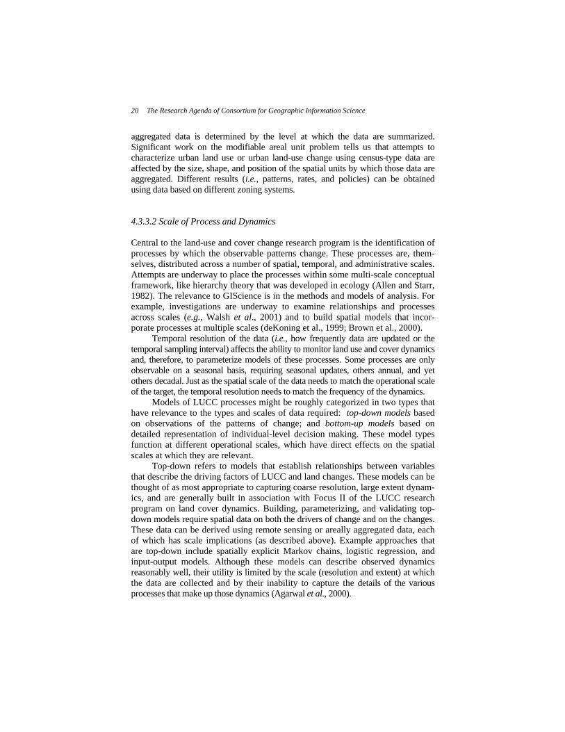
4.3.3.2 Scale of Process and Dynamics Central to the land-use and cover change research program is the identification of processes by which the observable patterns change. These processes are, them-selves, distributed across a number of spatial, temporal, and administrative scales. Attempts are underway to place the processes within some multi-scale conceptual framework, like hierarchy theory that was developed in ecology (Allen and Starr, 1982). The relevance to GIScience is in the methods and models of analysis. For example, investigations are underway to examine relationships and processes across scales (e.g., Walsh et al., 2001) and to build spatial models that incor-porate processes at multiple scales (deKoning et al., 1999; Brown et al., 2000).

Temporal resolution of the data (i.e., how frequently data are updated or the temporal sampling interval) affects the ability to monitor land use and cover dynamics and, therefore, to parameterize models of these processes. Some processes are only observable on a seasonal basis, requiring seasonal updates, others annual, and yet others decadal. Just as the spatial scale of the data needs to match the operational scale of the target, the temporal resolution needs to match the frequency of the dynamics.

Models of LUCC processes might be roughly categorized in two types that have relevance to the types and scales of data required: top-down models based on observations of the patterns of change; and bottom-up models based on detailed representation of individual-level decision making. These model types function at different operational scales, which have direct effects on the spatial scales at which they are relevant.

Top-down refers to models that establish relationships between variables that describe the driving factors of LUCC and land changes. These models can be thought of as most appropriate to capturing coarse resolution, large extent dynam-ics, and are generally built in association with Focus II of the LUCC research program on land cover dynamics. Building, parameterizing, and validating top-down models require spatial data on both the drivers of change and on the changes. These data can be derived using remote sensing or areally aggregated data, each of which has scale implications (as described above). Example approaches that are top-down include spatially explicit Markov chains, logistic regression, and input-output models. Although these models can describe observed dynamics reasonably well, their utility is limited by the scale (resolution and extent) at which the data are collected and by their inability to capture the details of the various processes that make up those dynamics (Agarwal et al., 2000).

Scale 21

Bottom-up refers to models that attempt to describe the important elemental components of the land-use change process, and build land-use and cover change descriptions up from these finer scale depictions. They are most commonly associated with work on Focus I of the LUCC research program on land-use dynamics. Although these models can be scaled to describe large areas, they require significant data and computational power to do so. Most bottom-up models to date cover relatively small extents. They rely on disaggregate data on individual-level decision making, where the individuals can be persons, house-holds, parcels, and units of government. These data might include landscape per-ception of people, household wealth and means of livelihood, and farmers’ evaluations of risk, etc. Cellular automata and agent-based models are examples of modeling approaches that address bottom-up dynamics. These models may offer a stronger platform for cross-scale integration, because the models can include processes at a variety of scales that impinge on agent behavior and can include agents that operate at a variety of scales.

Important scaling challenges involve the selection of appropriate models (i.e., top-down vs. bottom-up) for particular questions, settings, and scales. Furthermore, because processes and patterns operate at a variety of scales, integration of the top-down and bottom-up dynamics with data on fine-scale behavior (i.e., individual and collective human perceptions, behaviors, and decision making processes) and coarse-scale outcomes (i.e., changes in land-use and cover patterns) is important to the LUCC effort.

4.3.4 Environmental and Public Health The study of the environment in relation to health is inherently a geographical problem. As with other geographical problems, scale is a main factor contributing to the uncertainties of the analysis, hence our understanding of and decision-making about environmental and public health phenomena. This is especially true for those health risk assessment studies that involve the use of small areas. Small-area ecological studies in environmental health refer to studies that require data defined in fine spatial scale, such as census tracts, census blocks, and zip code districts. They typically involve data from disparate sources when intensive data pro-cessing and analysis is a characteristic. Therefore, they are amenable to GIS technology.

Small-area ecological studies explore the statistical connections between the frequency of a disease and the level of exposure to a particular agent in popu-lation groups rather than individuals (English, 1992). Disparate data sources, such as vital records, hospital discharges, disease registries, census, and estimates of exposure, are typically utilized in order to uncover relationships that most believe to occur and be detectable only at a finer scale (smaller spatial extent and finer spatial resolution). Historically, these types of geographical studies have provided important clues to the etiology of disease, as marked by the infamous example of the discovery of the cause of cholera in London by Dr. John Snow in 1890


(Elliott et al., 1992). Unlike case-control studies, small-area ecological studies seldom lead to definite conclusions about the causes of disease. However, ecological studies are especially suited to forming and refining hypotheses about etiology, which in turn could provide useful guidelines for case-control studies.

Although using small areas is almost a norm in environmental and public health studies, it is worthwhile to note that geographical studies at an inter-national scale have been successful in identifying broad relationships because they exploit large differences in both the frequency of the disease and the prevalence of exposure. The relationship between lack of sunlight and rickets is a good example (English, 1992). Using small areas to study rickets will unlikely reveal the relationship, as rates of disease and environmental exposures are likely to be homogeneous in a small geographical area. The large spatial extent (i.e., large geographical scale) thus plays an important role in uncovering the cause of this disease. As discussed below, this example also points to the need for study using a multi-scale approach, so that patterns and relationships can be determined with higher degree of certainty.

In general, small-area studies focus on four areas of inquiry: geographical correlation, mapping and visualization, the analysis of disease risk around a putative point source, and the assessment of spatial clustering. We provide below an example in each area of inquiry to illustrate how scale affects our under-standing of the phenomena and how policy making about the phenomena are subsequently impacted.

4.3.4.1 Geographical Correlation In a geographical correlation study of leukemia in Wisconsin, Cleek (1979) pointed out that correlations are more easily affected than regression coefficients by changes in data resolution and aggregation. As the individuals are aggregated into county level, socioeconomic measures are generalized. The coefficient of variation (standard deviation/mean) for mortality rates from leukemia was 7.0 percent comparing states at the national level and 20.9 percent comparing counties within the state of Wisconsin. Similarly the coefficient of variation of mortality rates for cancer of the nasopharynx is 188.9 percent for Wisconsin at the county level and 24.4 percent for the United States at the state level. Colon cancer, however, has higher state-level variation (25.8 percent) than county-level variation (17.3 percent). Cleek suggested using regression coefficients in report-ing and treating correlation coefficients with care (Meade and Earickson, 2000).

This study demonstrates that patterns of association are different at different spatial resolutions and spatial extents, and it is an error to infer an association from one level of scale to another. Especially in environmental and public health studies where the public is sensitive to those issues, caution must be taken in reporting and communicating the results to the public, and policy making based on these results will need to consider the various results at multiple scales.

Scale 23

Cleek’s study further shows that not all the variables respond the same way as spatial resolution decreases, such as colon cancer in the study, where higher aggregation level (i.e., coarser spatial resolution) does not necessary result in smoother distribution (or lower variation). The interaction between resolution, spatial extent, analysis method, and the phenomenon itself is complex, and strategies must be developed to systematically uncover such interaction.

4.3.4.2 Disease Mapping Mapping disease patterns is an effective means of summarizing and commu-nicating potential relationships. The production of cancer maps for many countries testifies to the appeal of this approach. A well-known example is the Chinese atlas of cancer mortality published in 1981, which showed distinct regional variation in cancer mortality for many cancer sites (The Atlas of Cancer Mortality in the People’s Republic of China, 1981; Lam, 1986). In the atlas, the sex-specific mortality rates of the nine most common cancers by county, based on data collected in 1973–75, were generalized and shown in the form of choropleth maps. There are many issues related to the mapping method itself, here we focus on the issues related to scale. In the case of esophagus cancer, the second most common cancer in China, the county-level map for male (Figure 4.12) shows distinct clustering in the central part of China. Clusters of high rates were also observed in remote counties located in the northern and northwestern part of China. However, when the mortality rates were aggregated and mapped at the provincial level (Figure 4.13), the spatial pattern becomes more generalized, and the clustering in the remote counties disappears in the provincial map. These counties could be important clues for studying the etiology of the disease.

In a related study that compares cancer mortality patterns at the provincial level for the entire country and a small region at the commune level (of finer resolution), Lam (1990) showed that the spatial autocorrelation statistics com-puted for the two map patterns were quite different. The spatial autocorrelation statistic computed for the esophagus cancer for male at the provincial level was found to be not significant at the 0.05 significance level. But when mapped at the commune level (on average, a county has about 30 communes), the spatial autocorrelation statistic indicates that the pattern is positively autocorrelated at the 0.05 significance level, implying the existence of a clustered pattern.

In an attempt to detect at which range of scales the relationship are alike and at what scale the patterns change, the fractal and variogram techniques were introduced to analyze the cancer mortality patterns in China (Lam et al., 1993). Variogram plots of three cancer patterns (esophageal, stomach, and liver) for the Taihu Region in China show that esophageal and liver cancers have the same self-similar scale ranges (roughly between 6 and 150 km), and they are larger than that of stomach cancer (roughly up to 100 km). These self-similar scale ranges were determined based on the portion of the curves that remain linear


Figure 4.12 Esophagus cancer mortality (1973–75) for male by county. Shaded counties are those that have high and significant mortality rates

(data source: The Atlas of Cancer Mortality in China, 1981)

Figure 4.13 Esophagus cancer mortality (1973–75) for male by province. Shaded provinces are those that have high and significant mortality rates

(data source: The Atlas of Cancer Mortality in China, 1981)

Scale 25

(Figure 4.14). These self-similar scale ranges could suggest that, if the communes are aggregated to a distance greater than the scale ranges, the map patterns could look very different that could lead to a different interpretation of the underlying processes. It was also speculated that whatever the underlying controlling factors (e.g., climate, topography, water source), they are likely to operate in ranges of scales similar to that of the cancer patterns.

Figure 4.14 Variogram plots of esophageal, stomach, and liver cancer mortality patterns for the

Taihu Region, China. The bars on each curve indicate the portion of the curves that remain linear, or in fractal terminology, the range of scales that are self-similar (from Lam et al., 1993)

4.3.4.3 Risk Assessment around a Source A common question in this area of inquiry is: do certain facilities or industrial sites (e.g., hazardous waste treatment plants) pose an adverse effect on the health of people living close by? This question has been asked over and over again. However, uncertainties involved in this type of health risk assessment studies are high, of which scale contributes an important part. Conflicting results can be generated from various factors, including definitions of data in different spatial and time scales. Consequently, conclusive statements on the impacts of hazardous industrial sites on human health are often lacking.

For example, the famous controversy on whether significant increase in leukemia incidence is related to nearby nuclear installation in England during the late 1980s has generated numerous studies and a disparity of results (Forman et al., 1987; Gardner, 1989). The techniques used in these studies varied: some used incidence while others used mortality; some used rates and compared observed with expected numbers while others used Poisson probabilities; some used existing administrative boundaries while others used circles of arbitrary


sizes drawn around a presumed source. Disease clusters can be easily made to appear or disappear, because of these various ways of data manipulations (Glass et al., 1968; Openshaw et al., 1988).

In a study of the health effects of a hazardous waste site on its nearby population in Louisiana, arbitrary circles of 1-mile and 2-mile radii were drawn around the waste site (Lam 2001). If the 1-mile proximity zone is used, then the region is found to have significantly elevated rates in certain cancers. But if the 2-mile proximity zone is used, then the results are reversed, and the cancer rates defined within the 2-mile wide circle are significantly lower. The dilemma is clear: which results should one adopt for reporting to the public and for deriving policies?

4.3.4.4 General Cluster Detection Detecting clusters of disease when there is no suspected source is a central, but probably most controversial, research problem in geographical epidemiology. There are many methods and models to detect spatial, temporal, and spatio-temporal clusters. The goal is to identify clusters of areas that are significant and merit further investigation, and at the same time, avoid unnecessary costly epidemiologic (e.g. case-control) studies if the clusters are found to be spurious (Marshall, 1991).

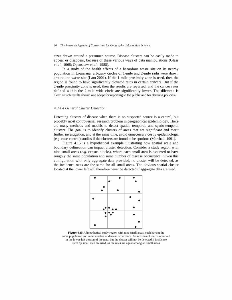
Figure 4.15 is a hypothetical example illustrating how spatial scale and boundary delineation can impact cluster detection. Consider a study region with nine small areas (e.g. census blocks), where each small area is assumed to have roughly the same population and same number of disease occurrence. Given this configuration with only aggregate data provided, no cluster will be detected, as the incidence rates are the same for all small areas. The obvious spatial cluster located at the lower left will therefore never be detected if aggregate data are used.

Figure 4.15 A hypothetical study region with nine small areas, each having the

same population and same number of disease occurrence. An obvious cluster is observed in the lower-left portion of the map, but the cluster will not be detected if incidence

rates by small area are used, as the rates are equal among all small areas

Scale 27

4.3.4.5 Strategies for Mitigating the Scale Effects As mentioned earlier, scale effects exist and can never be eliminated. Strategies must be developed to mitigate or reduce the scale effects. Two approaches to miti-gating the scale effects in health applications can be identified. First, emphasis is placed on developing techniques to detect at which range of scales the relationships are alike and at which other range of scales do things appear and act differently. Variogram, correlogram, and fractal analysis are some of the spatial techniques that have been proposed to detect the range of scales that yield the most information (i.e., scale of actions) (Lam, et al., 1996; Cao and Lam, 1997; Tate and Atkinson, 2001).

The other approach, which receives increasing attention from researchers, is to employ multi-scale analysis so that scale effects can be examined and uncer-tainties due to scale can be reduced. The Centers for Disease Control and Preven-tion (CDC, 1990) called for a systematic approach to investigating health outcomes. In response to the CDC call, Schneider et al. (1993) studied cancer clusters in New Jersey using data at multiple geographical scales. They concluded that analysis of cancer incidence data and cancer clusters at multiple geographic scales provides confidence of the results, alleviates fears of the general public, and prevents costly and unwarranted epidemiologic studies. Ozdenerol (2000) studied infant low birth weight in a typical American city (Baton Rouge, Louisiana) using data aggregated at three spatial scales–census tracts, block groups, and blocks. The results showed that spatial clustering existed in the same general location (inner city neighborhood) for all three scales. This type of multi-scale analysis provides more confidence on the findings. Lam (2001) proposed the use of an integrated spatial analysis frame-work to reduce uncertainties associated with health risk assessment studies, and scale analysis is a key component of the proposed framework. 4.4 RESEARCH PRIORITIES Issues of scale affect nearly every GIS application and involve questions of scale cognition, the scale or range of scales at which phenomena can be easily recognized, optimal digital representations, technology and methodology of data observation, generalization, and information communication. These are very dif-ferent types of questions, and have been addressed quite abundantly in different subfields and disciplines, including geography (Hudson, 1992), remote sensing (Quattrochi and Goodchild, 1997; Tate and Atkinson, 2001), cartography (Buttenfield and McMaster, 1991), spatial statistics (Wong and Amrhein, 1996), hydrology (Sivapalan and Kalma, 1995), and ecology (Ehleringer and Field, 1993).

Effective research in the area of scale will require interdisciplinary efforts of geographers, geostatisticians, cartographers, remote sensing specialists, domain experts, cognitive scientists, and computer scientists. Scale research in many insti-tutes, agencies, and in the private sector began in an ad hoc fashion. Motivated both by practical needs as well as theoretical development, recent attention is focused on

nlam

The


formalizing the study of scale, on developing theory, and on exploring robust methods for information representation, analysis, and communication across multiple scales.

It has become clear that global and regional processes have implications for local places and that individual and local decisions collectively have global and regional implications. Therefore, scientific information about global and regional patterns and processes must be understood on a local level and vice versa. As the policy-making and scientific communities come to terms with these relationships, systematic understanding about spatial and temporal variations in scale gain impor-tance. Geographical information plays an ever larger role as we move to an increas-ingly automated information economy. Our understanding of scale and the manage-ment of data at various scales must keep pace. Ultimately data and information must inform and must produce better decisions.

Based on the discussion above, a number of research priorities on scale can be outlined as follows.

• Definitions of scale concepts. There has been much confusion and misuse of the term “scale.” A summary of the meanings and scope of scale is provided in Section 4.2. However, more thorough work is needed to help clarify all connotations of scale in a multidisciplinary context. A good understanding of the conceptual relationship between these connotations should benefit the geographic information users in conjunction with other standardization efforts in geographic information use.

• Systematized bases for scale-related decision making. Basic research on the effects of scale on information content will yield practical infor-mation for the many users of geographical information. We need to ask, for example, if we lose a significant portion of our explanatory power when we represent global population trends by country as compared with representations at the level of primary divisions within countries. In an increasing array of management and policy settings, decisions about the appropriate scales of analysis are made every day. Identification of critical scales and of scale-invariant data sets or modeling procedures can make those decisions explicit and better informed.

• Practical guidance on data integration and use. Often, data at sub-optimal or disparate scales are the best available. Using imperfect data that are available is in many cases preferable to using no data at all, but there are implications for the validity of results. For the user community, creation of knowledge about scale provides principles to improve a data set’s fitness for use and guidelines by which to discount model results when necessary. For example, we already know that analysis using aggre-gate data cannot be used to impute the behavior of individuals (called the ecological fallacy). A better understanding of the problem of conflation (the procedure of merging the positions of corresponding features in different data layers) will enable the fusing of data sets, produced at different scales

Scale 29

or produced at the same scale but from different sources. Conflation currently poses a serious impediment in the map overlay process, a critical component of GIS. A better understanding of conflation is also necessary for the integration of data sets produced by different agencies.

• New methods for quantifying and compensating for the effects of scale in statistical and process models. Scientists and land managers apply a variety of analytical tools to answer geographic questions. Many existing methods do not allow the user to adjust or compensate for the effects of the data scale on the analysis results. Methods that are sensitive to scale will allow the inclusion of scale correctives, much like the correctives that compensate for inflation of the significance of statistical relationship in the presence of spatial autocorrelation.

• Intelligent automated generalization methods. GIS tools can be expanded to provide users with methods for intelligently changing the scale of their data. Basic research is still needed to understand how scale changes are perceived, and this in turn can inform interface design. Intelligent gener-alization will permit the encoding of raw observations in digital form to derive more responsive, application-specific representations.

• Improved understanding of cognitive issues of scale. Many scale ques-tions involve human cognition (i.e., how humans perceive the world and information representing it). This issue is explicit especially during human-computer interaction and must be dealt with technically during interface development. It ultimately affects a chain of decisions. Basic research lays a foundation for answering how humans perceive scale changes and its relationship with the conceptual and technical questions about the proper use of spatial and temporal scales in geographic information processing.

4.4.1 Potential Projects From the above broader research priorities, a number of potential projects are suggested:

• Develop more consistent definitions of scale and its associated attributes that can be uniformly understood or perceived across multiple disci-plines. The challenge here is how to make the “standardized” lexicon be adopted and utilized multidisciplinarily.

• Encourage the development of a scale analysis module to be included in major environmental analytical and measurement methods, so that sensitivity analysis, robustness testing, and the effects of scale on the analytical findings can be assessed.


• It is important to point out that many existing scale studies rely heavily on the resampling methods to generate multiscale data for analysis, and as such, the findings on the scale effects may not really be due to the scale effects, but rather they may be an artifact attributable to the use of different resampling methods (Weigel, 1996). The effects of resam-pling methods on the scale studies are an aspect requiring further research.

• More work needs to be done to identify, develop, and compare efficient spatial/geostatistical techniques for assessing and characterizing the scale effects. This includes refinement of existing techniques, such as fractals, spatial autocorrelation, Shannon index, geographical variance, and local variance, as well as exploration of new techniques such as wavelet analysis, local fractals, and multifractals (Mallat, 1989; Pecknold et al., 1997; Hou, 1998; Myint, 2001; Zhao, 2001). The indices derived from these techniques, if sufficiently discriminatory and information-rich, could be included as part of the metadata.

• Identify the ranges of scale over which an encoded attribute classi-fication scheme is valid. A project of this type will help build a better understanding of the linkages between the scale of a spatial repre-sentation and the appropriate corresponding attribute detail. For example, land cover data represented as 30-meter pixels should include more thematic detail (i.e., more number and types of classes) in the land cover classification than similar data represented as 1-kilometer pixels. Studies of these relationships in specific settings and for specific data sets will need to be performed with the aim of building theoretical bases for understanding these relationships more generally.

• Identify the optimal scales of analysis for common data sets, appli-cations, and needs, and critical scales at which the content or structure of phenomena change suddenly (e.g., in vegetation or population). This work will involve the application of sensitivity analyses and spatial statistical tools for describing those sensitivities. Ultimately the goal is to allow users of geographic data to determine the appropriate scales prior to data collection or analysis.

• Develop methods for cost-benefit analysis comparing the use of pregeneralized data (e.g., soil polygons) versus automated generalization of raw data (e.g., soil data from collection points). “Cost” could refer to data collection costs and/or to computational cycles; “benefits” can similarly serve as a metaphor for data validity; each will depend on the needs of the particular application. As automated generalization methods become readily available (many are now in commercial GIS packages), users may wish to access data in the rawest form possible as opposed to

Scale 31

using data generalized for a specific purpose. Research of this type would have implications for data collection and archival agencies as well as users.

• Develop improved methods for data generalization. A well researched, yet still unsolved, problem associated with spatial generalization is the creation of multiple versions of databases. Research in cartographic generalization has taken several directions including algorithmic design and testing, the design of models and conceptual frameworks, the appli-cation of expert systems, and the modeling of cartographic features. Thus far, most of the work in generalization has focused on what is termed “cartographic” generalization, which involves the graphical considerations associated with scale change. A second, less researched, area is in “model” generalization, by which generalization operators (simplification, smoothing, aggregation, agglomeration, and others) are applied to an original digital landscape model (DLM) in order to create secondary representations of the database, called digital cartographic models (DCM). These terms, DLM and DCM, are taken from the European cartographic literature, where a significant amount of work has been completed in this area.

• Develop improved methods for incorporating knowledge about scale into metadata. We need to model descriptive data about data sets (i.e., metadata) to assess the consequences of downloading data at a finer resolution than is needed for a particular GIS application. The question is to determine if the choice of appropriate scale can be made on the basis of metadata alone. With the expansion of global computer networks and the use of those networks for geographic data transmission, efficient modes of communicating data content are needed. We need to determine which modes are most appropriate for representing scale and to evaluate their relative effectiveness. The provision of information about scale aids in the education of users on how to assess appropriate scales for a given appli-cation. Scale is clearly a fundamental component of any metadata report.

• Design and develop a multi-scale database. We still lack the database management tools and associated functions needed to effectively and efficiently store multi-scale data, perform multi-scale analysis, and intelligently change scale. This project should be aimed at the develop-ment of a software product that would be useful in GIS applications.


4.5 REFERENCES Agarwal, C., G.L. Green, Grove, M., Evans T. and Schweik, C., 2000, A Review

and Assessment of Land-Use Change Models: Dynamics of Space, Time, and Human Choice, Bloomington, IN: CIPEC, Indiana University.

Allen, T.F.H. and Starr, T.B., 1982, Hierarchy: Perspectives for Ecological Complexity, Chicago: University of Chicago Press.

The Atlas of Cancer Mortality in the People’s Republic of China, 1979.Beijing: China Map Press.

Brown, D.G., Pijanowski, B.C. and Duh, J.D., 2000, Modeling the relationships between land-use and land-cover on private lands in the upper Midwest, USA. Journal of Environmental Management, 59: 247–163.

Buttenfield, B., 1984, Line Structure in Graphic and Geographic Space, Unpublished Ph. D. Dissertation, University of Washington.

Buttenfield, B.P. and McMaster, R.B. (eds.), 1991, Map Generalization: Making Rules for Knowledge Representation, New York: Longmont Scientific and Technical.

Cao, C.Y. and Lam, N.S.-N., 1997, Understanding the scale and resolution effects in remote sensing and GIS. In Quattrochi, D.A. and Goodchild, M.F. (eds.), Scale in Remote Sensing and GIS, Boca Raton, FL: CRC/Lewis Publishers, pp. 57–72.

Catts, D., 1990, Generalization of GIS digital maps. Papers and Proceedings of Applied Geography Conference, Binghamton, NY: Applied Geography Conference, Inc.

Centers for Disease Control and Prevention, 1990, Guidelines for investigating cluster of health events. Morbidity and Mortality Weekly Report, 39: 1–23.

Cihlar, J. and Jansen, L.J.M., 2001, From land cover to land use: A methodology for efficient land use mapping over large areas. The Professional Geographer, 53(2): 275–289.

Cleek, R.K., 1979, Cancer and the Environment. The Effect of Scale. Social Science and Medicine, 13D: 241–247.

Cromley, R.G., 1991, Hierarchical methods of line simplification. Cartography and Geographic Information System, 18: 125–131.

De Cola, L. and Buttenfield, B., 1994, Multiscale mapping for the NSDI: Data modeling and representation. Proceedings of GIS/LIS annual conference.

De Koning, G.H.J., Veldkamp, A. and Fresco, L.O., 1999, Exploring changes in Ecuadorian land use for food production and their effects on natural resources. Journal of Environmental Management, 57: 221–237.

Douglas, D. and Peucker, T., 1973, Algorithms for the reduction of the number of points required to represent a digitized line or its caricature. Canadian Geographer, 10(3): 112–122.

nlam

Proceedings

nlam

Buttenfield,

Scale 33

Ehleringer, J.R. and Field, C.B. (eds.), 1993, Scaling Physiological Processes, Leaf to Globe. New York: Academic Press.

Elliot, P., Cuzick, J., English, D. and Stern, R. (eds.), 1992, Geographical and Environmental Epidemiology: Methods for Small-Area Studies, Oxford: Oxford University Press.

Emerson, C.W., Lam, N.S.-N. and Quattrochi, D.A., 1999, Multi-scale fractal analysis of image texture and pattern. Photogrammetric Engineering and Remote Sensing, 65(1): 51–61.

English, D., 1992, Geographical epidemiology and ecological studies. In Elliot, P., Cuzick, J., English, D. and Stern, R. (eds.), Geographical and Environmental Epidemiology: Methods for Small-Area Studies, Oxford, UK: Oxford University Press, pp. 3–13.

ERITO, 1997 (last update), http://www.ertico.com/links/gdf/gdfintro/gdfincon.htm.

Forman, D., Cook-Mozaffari, P., Darby, S. and others, 1987, Cancer near nuclear installations. Nature, 329: 499–505.

Gardner, M.J., 1989, Review of reported increases of childhood cancer rates in the vicinity of nuclear installations in the UK. Journal of Royal Statistical Society A, 152: 307–325.

Glass, A.G., Hill, J.A. and. Miller, R.W., 1968, Significance of leukemia clusters. Journal of Pediatrics, 73: 101–107.

Hou, R.-R., 1998, A Local-Level Approach in Detecting Scale Effects on Landscape Indices, Baton Rouge, Louisiana: Louisiana State University. M.S. Thesis.

Hudson, J., 1992, Scale in space and time. In Abler, R.F., Markus, M.G. and Olson, J.M. (eds.), Geography’s Inner Worlds: Pervasive Themes in Contemporary Amer-ican Geography, New Brunswick, NJ: Rutgers University Press, pp. 280–300.

Kulldorff, M., 1997, A spatial scan statistic. Communications in Statistics: Theory and Methods, 26: 1,481–1,496.

Lam, N.S.-N., 1986, Geographical patterns of cancer mortality in China. Social Science and Medicine, 23(3): 241–247.

Lam, N.S.-N., 1990, The role of geographical scale in analyzing cancer mortality patterns in China. Paper presented at the 1990 IGU Regional Conference on Asian Pacific Countries, Beijing, China.

Lam, N.S.-N., 2001, Spatial analysis for reducing uncertainties in human health risk assessment. Acta Geographica Sinica, 56(2): 239–247. (In Chinese with English abstract).

Lam, N.S.-N., Qiu, H.L., Zhao, R. and Jiang, N., 1993, A fractal analysis of cancer mortality patterns in China. In. Lam, N.S.-N and De Cola, L. (eds.), Fractals in Geography, Englewood Cliffs, NJ: Prentice Hall, pp. 247–261.


Lam, N.S.-N. and Quattrochi, D.A., 1992, On the issues of scale, resolution, and fractal analysis in the mapping sciences. The Professional Geographer, 44(1): 88–98.

Lam, N.S.-N. and De Cola, L. (eds.), 1993, Fractals in Geography, Englewood Cliffs, NJ: Prentice Hall.

Lam, N.S.-N., Fan, M. and Liu, K.B., 1996, Use of space-filling curves in generating a national rural sampling frame for HIV/AIDS research. The Professional Geographer, 48(3): 321–332.

Lam, N.S-N., Quattrochi, D.A., Qiu, H.-L. and Zhao, W., 1998, Environmental assessment and monitoring with image characterization and modeling system using multiscale remote sensing data. Applied Geographic Studies, 2(2): 77–93.

MacEachren, A., 1995, How Maps Work, New York: The Guilford Press.

Mallat, S.G., 1989, A theory for multi-resolution signal decomposition: the wavelet representation. IEEE Transactions on Pattern Analysis and Machine Intelligence, 11: 674–93.

Marshall, R.J., 1991, A review of methods for the statistical analysis of spatial patterns of disease. Journal of Royal Statistical Society A, 154, Part 3: 421–441.

Meade, M.S. and Earickson, R.J., 2000, Medical Geography, New York: The Guilford Press.

Meentemeyer, V., 1989, Geographic perspectives of space, time, and scale. Landscape Ecology, 3(3/4): 88–98.

Meentemeyer, V. and. Box, E.O., 1987, Scale effects in landscape studies. In Turner, M.G. (ed.), Landscape Heterogeneity and Disturbance, New York: Springer-Verlag, pp. 15–34.

Muller, J., 1990, The removal of spatial conflicts in line generalization. Cartography and Geographic Information Systems, 17: 141–149.

Monmonier, M., 1991, How to Lie With Maps. Chicago: University of Chicago Press.

Montello, D.R. and Golledge, R.G., 1998, Summary Report: Scale and Detail in the Cognition of Geographic Information, NCGIA Report of Specialist Meeting held under the auspices of Project Varenius, May 14–16, 1998. University of California at Santa Barbara, 65 pp.

Moody, A. and Woodcock, C.E., 1995, The influence of scale and the spatial characteristics of landscapes on land-cover mapping using remote sensing. Landscape Ecology, 10(6): 363–379.

nlam

Maling, D., 1989, Measurements from Maps, Oxford, England: Pergamon Press.

nlam

McMaster, R. and Mark, D., 1991, The Design of a Graphical User Interface for Knowledge Acquisition in Cartographic Generalization. Proceedings of GIS/LIS, vol. 1.

Scale 35

Myint, S.W., 2001, Wavelet Analysis and Classification of Urban Environment Using High-Resolution Multispectral Image Data, Ph.D. Dissertation, Louisiana State University.

Nickerson, B., 1988, Automated cartographic generalization for linear features. Cartographica, 25(3): 15–66.

Oliver, M.A., 2001, Determining the spatial scale of variation in environmental properties using the variogram. In Tate, N.J. and Atkinson, P.M. (eds.), Modelling Scale in Geographical Information Science, Chichester, UK: John Wiley & Sons, pp. 193–220.

Openshaw, S., Charlatan, M., Wymer, C. and Craft, A., 1987, A Mark 1 geographic analysis machine for the automated analysis of point data sets. International Journal of Geographic Information Systems, 1(4): 335–358.

Openshaw, S., Craft, A.W., Charlton, M.G. and Birch, J.M., 1988, Investigation of leukemia clusters by use of a geographical analysis machine. Lancet Feb. 6: 272–273.

Ozdenerol, E., 2000, A Spatial Inquiry of Infant Low Birth Weight and Cancer Mortality in East Baton Rouge Parish, Louisiana. Ph.D. Dissertation, Louisiana State University.

Pecknold, S., Lovejoy, S., Schertzer, D. and Hooge, C., 1997, Multifractals and resolution dependence of remotely sensed data: GSI to GIS. In Quattrochi, D.A. and Goodchild, M.F. (eds.), Scale in Remote Sensing and GIS, Boca Raton, FL: CRC/Lewis Publishers, pp. 361–394.

Quattrochi, D.A., 1993, The need for a lexicon of scale terms in integration ofremote sensing data with geographic information systems. Journal of Geography, 92(5): 206–212.

Quattrochi, D.A. and Goodchild, M.F. (eds.), 1997, Scaling in Remote Sensing and GIS, Boca Raton, FL: CRC/Lewis Publishers, Inc.

Quattrochi, D.A. and Goel, N.S., 1995, Spatial and temporal scaling of thermal infrared remote sensing data. Remote Sensing Reviews, 12: 255–286.

Quattrochi, D.A., Emerson, C.W., Lam, N.S-N. and Qiu, H-L., 2001, Fractal characterization of multitemporal remote sensing data. In Tate, N.J. and Atkinson, P.M. (eds.), Modelling Scale in Geographical Information Science, John Wiley & Sons: Chichester, UK, pp 13–34.

Qiu, H-L., Lam, N.S-N., Quattrochi, D.A. and Gamon, J.A., 1999, Fractal characterization of hyperspectral imagery. Photogrammetric Engineering and Remote Sensing, 65(1): 63–71.

Robinson, A., Morrison, J., Muehrcke, P., Kimerling, A.J. and Guptill, S.C., 1995, Elements of Cartography, 6th edition, New York: Wiley.

nlam

Ph.D. Dissertation, Louisiana State University.

nlam

of


Rodriguez, A., 1998–99, USFS GSTC Salt Lake, Utah, personal commun.

Sivapalan, M. and Kalma, J.D., 1995, Scale problems in hydrology: Contributions of the Robertson workshop. Hydrological Processes, 9(3/4): 243–250.

Skole, D.L. and Tucker, C.J., 1993, Tropical deforestation and habitat fragmen-tation in the Amazon: Satellite data from 1978 to 1988. Science, 260: 1,905–1,910.

Schneider, D., Greenberg, M.R., Donaldson, M.H. and Choi, D., 1993, Cancer clusters: The importance of monitoring multiple geographical scales. Social Science and Medicine, 37(6): 753–759.

Tate, N.J. and Atkinson, P.M. (eds.), 2001, Modelling Scale in Geographical Information Science, Chichester, UK: John Wiley & Sons.

Tobler, W. 1970, A computer movie simulating urban growth in the Detroit region. Economic Geography, 46 (Supplement): 234–240.

Tobler, W. 1988, Resolution, resampling and all that. In Mounsey, H. and Tomlinson, R. (eds.), Databases for Global Science, London: Taylor & Francis, pp. 129–137.

Turner, B.L., Skole, D., Sanderson, S., Fischer, G., Fresco, L. and Leemans, R., 1995, Land-Use and Land-Cover Change Science/Research Plan, Joint publi-cation of the International Geosphere-Biosphere Programme (Report No. 35) and the Human Dimensions of Global Environmental Change Programme (Report No. 7), Stockholm: Royal Swedish Academy of Sciences.

Turner, M.G., O’Neill, R.V., Gardner, R.H. and Milne, B.T., 1989, Effects of changing spatial scale on the analysis of landscape pattern. Landscape Ecology, 3: 153–162.

Walsh, S.J., Crawford, T.W., Welsh, W.F. and Crews-Meyer, K.A., 2001. A multi-scale analysis of LULC and NDVI variation in Nang Rong District, Northeast Thailand. Agriculture Ecosystems and Environment, 85(1-3): 47–64.

Weigel, S.J., 1996, Scale, Resolution and Resampling: Representation and Analysis of Remotely Sensed Landscapes Across Scale in Geographic Infor-mation Systems, Ph. D. Dissertation, Louisiana State University.

Wong, D. and Amrhein, C. (eds.), 1996, The Modifiable Areal Unit Problem. Special issue of Geographic Information Systems 3: 2–3.

Zhao, W., 2001, Multiscale Analysis for Characterization of Remotely Sensed Images, Ph.D. Dissertation, Louisiana State University.

nlam

Snyder, J.P., 1987, Map Projections—A Working Manual. USGS Professional Paper 1395, pages 22–23. Snyder, J.P., 1989, An Album of Map Projections. USGS Professional Paper 1453.

nlam

Wellge, H., 1884, Butte-City, Montana, J.J. Stoner, Madison, Wisconsin. Wilford, J.N., 1981, The Map Makers, A. A. Knopf, New York.

Documents

SCALE - University of Michigandanbrown/papers/scale_chapter.pdf · CHAPTER FOUR SCALE ... how to automate scale change and simultaneously represent data at ... graphic models that