Scale space vector fields for symmetry detection

Scale space vector fields for symmetry detection

Andrew D.J. Cross, Edwin R. Hancock*

Department of Computer Science, University of York, York, Y01 5DD, UK

Received 10 July 1997; received in revised form 10 March 1998; accepted 5 May 1998

Abstract

This paper describes a vectorial representation that can be used to assess the symmetry of objects in 2D images. The method exploits thecalculus of vector fields. Commencing from the gradient field extracted from filtered grey-scale images we construct a vector potential. Ourimage representation is based on the distribution of tangential gradient vectors residing on the image plane. By embedding the image plane inan augmented 3-dimensional space, we compute the vector potential by performing volume integration over the distribution of edge tangents.The associated vector field is computed by taking the curl of the vector potential. The auxiliary spatial dimension provides a natural scale-space sampling of the generating edge-tangent distribution; as the height above the image plane is increased, so the volume over whichaveraging is effected also increases. We extract edge and symmetry lines through a topographic analysis of the vector-field at various heightsabove the image plane. Symmetry axes are lines of where the curl of the vector potential vanishes; at edges the divergence of the vectorpotential vanishes.q 1999 Elsevier Science B.V. All rights reserved.

Keywords:Vector fields; Symmetry detection; Continuous symmetry; Canny edge-map

1. Introduction

Symmetry is an important way of assessing the shape ofboth 2D and 3D objects. Several alternative ways of locatingaxes and points of symmetry have been suggested in theliterature. Broadly speaking, these can be divided intothose that aim to analyse the properties of pre-segmentedshapes [1–5] and those that aim to characterize shape as acontinuous attribute [6–10]. Examples of the segmentalanalysis of symmetry include Friedberg’s moment-basedmethod [11], the use of spline-based representations byCham and Cipolla [2], Ponce’s idea of exploiting ribbons[3], and the skeletal analysis of binary shapes by Wright etal. [5]. The basic practical limitation of such methods is theavailability of reliable segmental entities prior to symmetryanalysis. It is for this reason that the early analysis of con-tinuous symmetry proves an attractive alternative. Forinstance Zabrodsky et al. have characterized the foldingsymmetries of 2D shapes using point-sets [8–10]. Reisfeldet al. generate a continuous symmetry measure from theorientation distribution for edgels and textons [6,7,12].

We make two observations concerning the existing workon continuous symmetry characterization. Firstly, the input

image representation is a sparse pre-segmentation, e.g.points of curvature, edgels or textons. Secondly, existingwork shares the common feature of using only a scalarrepresentation to assess symmetry structure. Our standpointin this paper is that a vectorial representation of the unseg-mented image data offers a more elegant way of assessingthe axial symmetries of planar shapes. This is a natural wayin which to proceed since the edge tangent vectors asso-ciated with the boundaries of regular 2D shapes exhibitchiral symmetry. At points of symmetry there is a cancella-tion of diametrically placed vectors. To exploit this prop-erty, we appeal to the mathematical concept of vectorpotential. The potential is found by volume averaging theedge tangent vectors. Individual vectors are weighted bytheir inverse distance from the sampling position. Asso-ciated with the potential is a vector field which is computedby taking its curl. The motivation underpinning this paper isthat although vector calculus has been widely exploited inthe analysis of scalar image representations, there has beenlittle effort devoted to the analysis of vector-field represen-tations of early visual feature formation.

Our aim in this paper is to develop vectorial theory ofcontour symmetry in 2D images. Although several authorshave exploited electrostatic field analogies in the analysis ofshape, these are less ambitious than the work reported heresince they are electrostatic in origin [13,14]. For instance,

0262-8856/99/$ - see front matterq 1999 Elsevier Science B.V. All rights reservedPII: S0262-8856(98)00133-4

* Corresponding author.E-mail address:[email protected] (E.R. Hancock)

Image and Vision Computing 17 (1999) 337–345

Wu and Levine have used charge distributions to segmentvolumetric objects into shape primitives [14]. The work ofAbdel-Hamid et al. [13] aims to find symmetry axes byseeding a charge distribution along a binary boundary con-tour and computing the lines of equipotential in the resultingelectric field. Our work differs from this related work in twoimportant respects. Firstly, we do not require a pre-segmen-ted surface or boundary from which to seed the generatingdistribution. Instead, we seed our field from the raw imagegradient. Secondly, the resulting vector field is generated bytaking the curl of the vector potential rather than the gradi-ent of a scalar potential. The resulting vector field has amuch richer differential structure which allows us to extractboth source lines (edges) and symmetry lines. Moreover, thechirality of the curl operator means that the resulting vectorfield has a mathematical structure that is better suited to theassessment of axial symmetry than the gradient of a scalarpotential.

Our basic idea is to regard edge tangent-vectors as a rawfeature distribution residing in the image plane. Thesevectors are computed by taking the cross-product of theimage gradient with the normal to the image plane. Inorder to compute the vector field we augment the 2Dimage space with an auxiliary vertical dimension. Foreach point in the resulting volume we compute the vectorpotential by integrating over the edge tangent distributionresiding on the embedded image plane. Following thedefinition of vector potential, the edge-tangent distributionis weighted by the inverse distance between the relevantsampling point in the augmented image volume and thepoints on the original image plane. The vector field is thecurl of the resulting vector potential. The auxiliary dimen-sion plays an important role in our image representation. Asthe height of the sampling plane above the image isincreased, the effective integrating volume increases. Thiscan be regarded as performing a role analogous to scale-space filtering [15–18]. The greater the height at which thevector-potential is sampled, the greater the smoothing effecton the original image.

We use the vertically sampled vector potential to extract arepresentation of the raw tangent-vector field. We are inter-ested in characterizing both edge and symmetry lines. Edgesare lines of maximum local vector potential since they cor-respond to the points where mutually aligned edge tangentsmaximally re-enforce one another. Symmetry lines corre-spond to the local minima of vector potential. Specifically,they represent contours where there is maximum cancella-tion of the vector potential associated with symmetricallyplaced edge-tangent vectors. An analysis of the associatedvector field reveals that field lines make tangential contactwith the sampling plane at the locations of edges. Symmetryaxes connect locations where the field lines are perpendicu-lar to the sampling plane. In terms of the differential struc-ture of the vector potential, symmetry points arecharacterized by zero curl whereas edge points are charac-terized by zero divergence. For reasons of computational

expediency we localize edge and symmetry lines byperforming a topographic analysis of the vector potential.The edges are crest lines while the symmetry lines are valleylines.

The outline of this paper is as follows. In Section 2 wedetail the basic image representation and describe how it isexploited to compute a vector potential from the raw imagegradient. Section 3 describes our analysis of the resultingvector field. Practical details of implementation are furn-ished in Section 4. In Section 5 we present an experimentalevaluation. Finally, Section 6 provides some conclusionsand outlines our future plans.

2. Vector field

Our starting point is to compute the Canny edge map [19].We commence by convolving the raw imageI with aGaussian kernel of widthj. The kernel takes the followingform

Gj(x, y) ¼1

2pjexp ¹

x2 þ y2

2j2

� �(1)

With the filtered image to hand, the Canny edge map isrecovered by computing the gradient

E¼ =Gj p I (2)

In order to compute a vector field representation of the edgemap, we will need to introduce an auxiliaryz dimension tothe originalx–y coordinate system of the plane image. Inthis augmented coordinate system, the components of theedge map are confined to the image plane. In other words,the edge vector at the point (x,y,0) on the input image planeis given by

E(x,y, 0) ¼

]Gj p I (x,y)]x

]Gj p I (x,y)]y

0

0BBBBB@

1CCCCCA (3)

For an ideal step-edge, the resulting image gradient will bedirected along the boundary normal. In order to pursue ourvectorial analysis of symmetry we would like to interpretthe raw edge responses as elementary tangents which flowaround the boundaries and give rise to a vector potential. Inparticular we would like to explore configurations in whichclosed boundary edges give rise to edge-tangent loops ortraces. In other words, we would like to organize the ele-mentary image gradients so that they are tangential to theboundaries of physical objects. Accordingly, we redirect theedge vectors so that they are tangential to the original planarshape by computing the cross-product with the normal to theimage planez¼ (0,0, 1)T. The elementary tangent vector atthe point (x,y,0) on the input image plane is defined to be

j(x, y,0) ¼ z ∧ =Gj p I (x,y) (4)

338 A.D.J. Cross, E.R. Hancock / Image and Vision Computing 17 (1999) 337–345

To be more explicit, the components of this elementarytangent are given by the vector

j(x,y, 0) ¼

¹]Gj p I (x,y)

]y

]Gj p I (x,y)]x0

0BBBBB@

1CCCCCA (5)

The vector potential associated with a field of elementarytangent vectors is found by integrating over volume andweighting the contributing vectors according to inverse dis-tance. In other words, the vector potential at the pointr ¼ (x, y,z)T in the augmented space in which the originalimage plane is embedded is

A(x,y, z) ¼

∫V9

j(r9)lr ¹ r9l

dV9 (6)

wherer9 ¼ (x9,y9, z9)T. Since the contributing edge tangentsare distributed only on the image plane, the volume integralreduces to an area integral over the image plane. As a result,the components of the vector potential are as follows

A(x,y, z)

¼

¹

∫∫ ]Gj p I (x9, y9)]y9

1��(x¹ x9)2 þ (y¹ y9)2 þ z2

p dx9 dy9

∫∫ ]Gj p I (x9, y9)]x9

1��(x¹ x9)2 þ (y¹ y9)2 þ z2

p dx9 dy9

0

0BBBBBBBB@

1CCCCCCCCAð7Þ

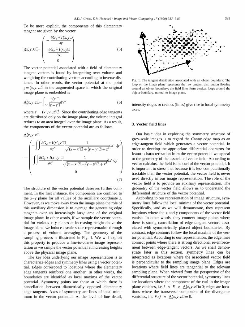
The structure of the vector potential deserves further com-ment. In the first instance, the components are confined tothe x–y plane for all values of the auxiliary coordinatez.However, as we move away from the image plane the role ofthis auxiliary dimension is to average the generating edgetangents over an increasingly large area of the originalimage plane. In other words, if we sample the vector poten-tial for variousx–y planes at increasing height above theimage plane, we induce a scale-space representation througha process of volume averaging. The geometry of thesampling process is illustrated in Fig. 1. We will exploitthis property to produce a fine-to-coarse image represen-tation as we sample the vector potential at increasing heightsabove the physical image plane.

The key idea underlying our image representation is tocharacterize edges and symmetry lines using a vector poten-tial. Edges correspond to locations where the elementaryedge tangents reinforce one another. In other words, theboundaries are identified as local maxima of the vectorpotential. Symmetry points are those at which there iscancellation between diametrically opposed elementaryedge tangents. Axes of symmetry are lines of local mini-mum in the vector potential. At the level of fine detail,

intensity ridges or ravines (lines) give rise to local symmetryaxes.

3. Vector field lines

Our basic idea in exploring the symmetry structure ofgrey-scale images is to regard the Canny edge map as anedge-tangent field which generates a vector potential. Inorder to develop the appropriate differential operators forfeature characterization from the vector potential we appealto the geometry of the associated vector field. According tovector calculus, the field is the curl of the vector potential. Itis important to stress that because it is less computationallytractable than the vector potential, the vector field is neverused directly in our image representation. The role of thevector field is to provide an auxiliary representation. Thegeometry of the vector field allows us to understand thedifferential structure of the vector potential.

According to our representation of image structure, sym-metry lines follow the local minima of the vector potential.Specifically, and as we will demonstrate, they representlocations where thex andy components of the vector fieldvanish. In other words, they connect image points wherethere is strong cancellation of edge tangent vectors asso-ciated with symmetrically placed object boundaries. Bycontrast, edge contours follow the local maxima of the vec-tor potential. According to our representation, the edge linesconnect points where there is strong directional re-enforce-ment between edge-tangent vectors. As we shall demon-strate later in this section, symmetry lines can beinterpreted as locations where the associated vector fieldis perpendicular to the sampling image plane. Edges arelocations where field lines are tangential to the relevantsampling plane. When viewed from the perspective of thedifferential structure of the vector potential, symmetry linesare locations where the component of the curl in the imageplane vanishes, i.e.z ∧ = ∧ A(x, y,z) ¼ 0; edges are loca-tions where the transverse component of the divergencevanishes, i.e.=:(z ∧ A(x, y,z)) ¼ 0.

Fig. 1. The tangent distribution associated with an object boundary: Theloop on the image plane represents the raw tangent distribution flowingaround an object boundary; the field lines form vertical loops around theobject-boundary, normal to image plane.

339A.D.J. Cross, E.R. Hancock / Image and Vision Computing 17 (1999) 337–345

3.1. The vector field

Although, we do not use it directly in our image repre-sentations, the natural extension of the development of thevector potential is to compute the associated vector field.Again, according to vector calculus this quantity is obtainedby computing the curl of the vector potential

B(x,y,z) ¼ = ∧ A(x,y,z) (8)

With the planar edge-tangent field described in the previoussection, the components of the vector field are related to thefiltered image gradient in the following way

Unfortunately, searching for scale-space edges or symmetrylines by directly exploring the differential geometry of thevector field is not a feasible computational proposition.Instead, we confine our attention to searching efficientlyfor local extrema of the vector potential on individual planesof fixed heightzabove the input image. As mentioned in thepreamble to this section, we represent the structure presentin the original image gradient field by identifying lines ofboth maximum and minimum vector potential. In practice,we characterize these lines by seeking ridges and ravines inthe topographic representation of the vector potential. Werealise this process by fitting a second-order polynomialprism surface to the magnitudes of the vector potential ina local image window. The prism surface is oriented alongthe direction of the vector potential. The maxima andminima are marked by testing for convexity or concavityof the fitted surface. This fitting procedure is similar to thatadopted by Spacek in his gradient-based edge detector [20].

3.2. Edge lines

Before we proceed to experiment with our new symmetrydetector, we will provide some analysis of the properties ofthe underlying image representation. The simplest case is toconsider the properties of edge lines. The localizationprocess is effected by identifying points for which thetransverse derivative of the vector potential is zero. Inother words we compute the derivatives of the vector poten-tial in the direction which is perpendicular toA(x, y,z) and

which lies in thex–y plane. The condition for edge lines is

=:(z ∧ A(x, y,z)) ¼ 0 (10)

Using standard identities from vector calculus, the requiredderivatives are related to the curl of the vector potential inthe following manner

=:(z ∧ A(x, y,z)) ¼ A(x, y,z):= ∧ z¹ z:(= ∧ A(x,y, z))(11)

Sincez is a constant vector, i.e.= ∧ z¼ 0, it follows that

=:(z ∧ A(x, y,z)) ¼ ¹ z:(= ∧ A(x,y,z)) (12)

Edge lines simply connect points for where thez-componentof the vector field vanishes, i.e.

z:B(x,y, x) ¼ 0 (13)

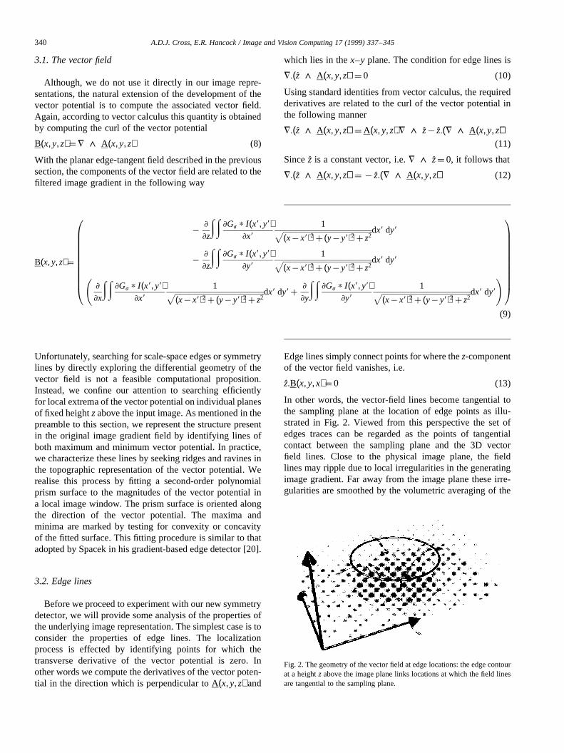
In other words, the vector-field lines become tangential tothe sampling plane at the location of edge points as illu-strated in Fig. 2. Viewed from this perspective the set ofedges traces can be regarded as the points of tangentialcontact between the sampling plane and the 3D vectorfield lines. Close to the physical image plane, the fieldlines may ripple due to local irregularities in the generatingimage gradient. Far away from the image plane these irre-gularities are smoothed by the volumetric averaging of the

B(x, y,z) ¼

¹]

]z

∫∫ ]Gj p I (x9,y9)]x9

1��(x¹ x9)2 þ (y¹ y9)2 þ z2

p dx9 dy9

¹]

]z

∫∫ ]Gj p I (x9, y9)]y9

1��(x¹ x9)2 þ (y¹ y9)2 þ z2

p dx9 dy9

]

]x

∫∫ ]Gj p I (x9, y9)]x9

1��(x¹ x9)2 þ (y¹ y9)2 þ z2

p dx9 dy9 þ]

]y

∫∫ ]Gj p I (x9, y9)]y9

1��(x¹ x9)2 þ (y¹ y9)2 þ z2

p dx9 dy9

!

0BBBBBBBBBB@

1CCCCCCCCCCA(9)

Fig. 2. The geometry of the vector field at edge locations: the edge contourat a heightz above the image plane links locations at which the field linesare tangential to the sampling plane.


vector potential. Noisy tangent fields are smoothed withincreasing height above the image plane.

In terms of the gradient of the original image, the edgelines satisfy the following condition

]

]x

∫∫ ]Gj p I (x9,y9)]x9

1��(x¹ x9)2 þ (y¹ y9)2 þ z2

p dx9 dy9 þ

(14)

]

]y

∫∫ ]Gj p I (x9,y9)]y9

1��(x¹ x9)2 þ (y¹ y9)2 þ z2

p dx9 dy9 ¼ 0

This condition can be viewed as an averaging of theLaplacian operator over a scale dictated by the samplingheight z. Moreover, our definition of an edge clearly hasan intimate relationship with the zero-crossings of theLaplacian operator.

3.3. Symmetry lines

This geometric analysis of the vector field can beextended to symmetry lines. Symmetry points occurwhere there is local cancellation of the vector potentialdue to a balanced edge-tangent flow around an objectboundary. At such points the vector field lines are ortho-gonal to the sampling plane. To understand the implicationof this statement in terms of differential operators, we notethat the condition for orthogonality of the vector field linesis

z ∧ B(x,y,z) ¼ 0 (15)

Using the definition of the vector field in terms of thevector potential and exploiting the identities of vectorcalculus

z ∧ = ∧ A(x,y,z) ¼ =(z:A(x,y,z))

þ = ∧ (z ∧ A(x,y, z)) ¹ (z:=)A(x,y,z) ð16Þ

SinceA(x, y,z) is confined to the image planez:A(x, y,z) ¼ 0and hence=(z:A(x, y,z)) ¼ 0. By direct substitution, it is astraightforward matter to show that

z ∧ = ∧ A(x,y,z) ¼

¹]

]zAx(x,y,z)

¹]

]zAy(x,y,z)

0

0BBBBB@

1CCCCCA (17)

whereAx(x, y,z) andAy(x, y,z) are thex andy componentsof the vector potentialA(x, y,z). In terms of the image

gradient

z ∧ = ∧ A(x,y, z)

¼

¹]

]z

∫∫]Gj p I (x9, y9)

]x9

1��(x¹ x9)2 þ (y¹ y9)2 þ z2

p dx9 dy9

¹]

]z

∫∫]Gj p I (x9, y9)

]y9

1��(x¹ x9)2 þ (y¹ y9)2 þ z2

p dx9 dy9

0

0BBBBBBBB@

1CCCCCCCCAð18Þ

In other words, the vectorz ∧ = ∧ A(x, y, z) is null alonglines for which the vertical derivative of tangent density iszero. We have therefore demonstrated that the symmetrylines are orthogonal to the sampling planes.

4. Implementation

In this section we will describe how the symmetry detec-tion process presented in this paper can be implemented inan efficient way. There are two aspects that deserve specialcomment. In the first instance we consider howx–y compo-nents of the vector potential can be efficiently computed.Key to our implementation is the fact that the volume inte-grals appearing in the definition of the vector potential (Eq.(7)) can be replaced by spatial-convolutions with a height-dependent filter. Specifically, we invoke the Fourier dualitybetween convolution in the spatial domain and multiplica-tion in the frequency domain. In this way the discretizedversion of the vector potential can be computed using justthree 2D Fourier transforms and a pair of frequency-domainconvolutions. The second implementational requirement isa means of localizing edge and symmetry features. For rea-sons of simplicity, we realise this process by searching forridges and ravines in the magnitude of the vector potential.Following Haralick and Laffrey [21] the required topo-graphic features are localized by fitting quadric patches.

4.1. Field computation

Our basic goal is to compute the vector potential at agiven height above the image plane. The two dimensionalintegrals appearing in the definition of vector potential canbe discretized to give the followingx andy components

Ax(x,y,z) ¼ ¹∑x9

∑y9

]Gj p I (x9,y9)]y9

31��

(x¹ x9)2 þ (y¹ y9)2 þ z2p ð19Þ

Ay(x,y,z) ¼∑x9

∑y9

]Gj p I (x9,y9)]x9

31��

(x¹ x9)2 þ (y¹ y9)2 þ z2p ð20Þ


The double summation can be replaced by a convolutionwith a composite filter. For instance, thex-component ofthe vector potential is as follows

Ax(x,y,z) ¼ ¹ (Vx(j,z) p I )(x,y) (21)

We exploit the commutative properties of convolution tocompute the composite filterVx(j,z). The filter is foundby convolving the appropriate directional derivative of theGaussian with the inverse Euclidean distance operator, i.e.

Vx(j, z)(x, y) ¼∑x9

∑y9

]Gj(x9, y9)]y9

1��(x¹ x9)2 þ (y¹ y9)2 þ z2

p(22)

For practical reasons, we would like to realise the computa-tion of the components of the vector potential using fastFourier transforms. Our basic strategy is to exploit the Four-ier duality between convolution in the spatial domain andmultiplication in the frequency domain. Schematically, weutilize the identity

Ax ¼ F ¹ 1 F [Vx(j,z)] 3 F [I ]� �

(23)

to compute each of the components of the vector potential inturn. In this way the vector potential can be obtained usingthree separate Fourier transform operations. The first ofthese involves computing the Fourier transform of the rawimageF [I ]. Two separate weighted spatial frequency dis-tributions are then constructed by multiplying the compo-nents of the image Fourier transform with the Fourierrepresentation for each of the composite filters in turn, i.e.we computeF [Ax(j, z)] and F [Ay(j,z)]. Finally, the twospatial components of the vector potential are obtained byinverse Fourier transformation of the two weighted fre-quency distributions. When this process is implementedusing fast Fourier transforms, then the time complexity isof the order(N ln(N))2 whereN is the image dimension. Infact, we have implemented the algorithm on an SGI Indyworkstation where it is capable of processing 2563 256pixel images at the rate of 25 frames per second. Finally, it isimportant to stress that our Fourier implementation is basedon a doubly toroidal image representation where there iswrap-around in thex andy directions of the pixel lattice.

4.2. Ridge and valley extraction

Once the magnitude of the vector potential is to hand, weneed to find the ridges and valleys in order to locate the edgeand symmetry features. Although the literature aboundswith many sophisticated algorithms for the analysis of topo-graphic image structure, we adopt a very simple procedurewhich has many features in common with the classical non-maximum suppression operator employed in the thinning ofdirectional edge-features [19].

We commence by fitting a local quadratic prism surfaceto the magnitude of the vector potential in each 33 3 imageneighbourhood. The direction of the prism returns a local

estimate for the orientation of the associated image feature.The curvature of the prism is indicative of the feature type.In the case of edge features the surface is convex while forsymmetry features it is concave. In the case of edge-featureswe use non-maximum suppression to test for localdirectional consistency of the detected ridges in the magni-tude of the vector potential. An analogous non-minimumsuppression test is applied to mark directionally consistentsymmetry features.

We acknowledge that this topographic analysis is crudeand leaves considerable scope for further improvement. Forinstance, we have not directly used the directional informa-tion in the vector potential, choosing instead to fit prismsurfaces to the magnitude alone. Moreover, we haveconsidered only parabolic lines (those for which Gaussiancurvature is zero and the mean curvature is non-zero). It isclear that the differential structure is much richer. Forinstance, the saddle-points of the magnitude are associatedwith corners in the grey-scale image. Suffice it to say thatthe implementation presented here has been primarily aimedat demonstrating some of the potential of our new represen-tation. We are currently refining both the differential analy-sis and the numerical realisation. Further results will bereported in due course.

5. Experiments

In this section we present an experimental evaluation ofour new feature characterization technique. We commenceby showing some examples for synthetic data. The aim hereis to illustrate some of the characteristics of the vectorpotential in simple situations. Our real-world evaluation ofthe method is more ambitious. The bulk of this experimen-tation is conducted using low-quality imagery delivered byan SGI IndyCam.

5.1. Artificial imagery

Before we proceed to experiment with real-world data,we pause to illustrate some of the properties of our vectorpotential on synthetic data. Fig. 3(a) shows a noisecorrupted letter ‘‘A’’. In Fig. 3(b) we show the locatededges in blue with the symmetry lines in red. The internalsymmetry lines fall roughly along the medial axis of thefigure. It is also important to note that there are alsosymmetry lines external to the figure. For instance, thereare three axes associated with the triangle enclosed by theupper half of the letter ‘‘A’’. These three axes intersect at apoint. There are also a number of lines associated with thetoroidal wrap-around used in our Fourier implementation ofthe convolution operations.

In Fig. 3(c), we turn our attention to the topography of themagnitude of the vector potential. Here we plot the value oflA(x,y, z)l. The figure illustrates the ridge-like character ofthe edges and the ravine-like character of symmetry axes.


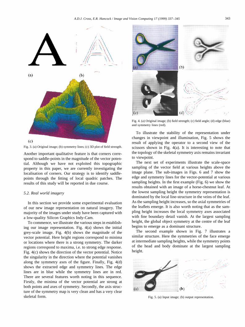
Another important qualitative feature is that corners corre-spond to saddle-points in the magnitude of the vector poten-tial. Although we have not exploited this topographicproperty in this paper, we are currently investigating thelocalisation of corners. Our strategy is to identify saddle-points through the fitting of local quadric patches. Theresults of this study will be reported in due course.

5.2. Real world imagery

In this section we provide some experimental evaluationof our new image representation on natural imagery. Themajority of the images under study have been captured witha low-quality Silicon Graphics Indy-Cam.

To commence, we illustrate the various steps in establish-ing our image representation. Fig. 4(a) shows the initialgrey-scale image. Fig. 4(b) shows the magnitude of thevector potential. Here bright regions correspond to minimaor locations where there is a strong symmetry. The darkerregions correspond to maxima, i.e. to strong edge response.Fig. 4(c) shows the direction of the vector potential. Noticethe singularity in the direction where the potential vanishesalong the symmetry axes of the figure. Finally, Fig. 4(d)shows the extracted edge and symmetry lines. The edgelines are in blue while the symmetry lines are in red.There are several features worth noting in this sequence.Firstly, the minima of the vector potential are strong atboth points and axes of symmetry. Secondly, the axis struc-ture of the symmetry map is very clean and has a very clearskeletal form.

To illustrate the stability of the representation underchanges in viewpoint and illumination, Fig. 5 shows theresult of applying the operator to a second view of thescissors shown in Fig. 4(a). It is interesting to note thatthe topology of the skeletal symmetry axis remains invariantto viewpoint.

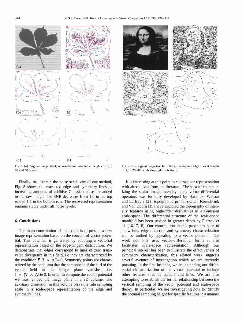
The next set of experiments illustrate the scale-spacesampling of the vector field at various heights above theimage plane. The sub-images in Figs. 6 and 7 show theedge and symmetry lines for the vector-potential at varioussampling heights. In the first example (Fig. 6) we show theresults obtained with an image of a horse-chestnut leaf. Atthe lowest sampling height the symmetry representation isdominated by the local line-structure in the veins of the leaf.As the sampling height increases, so the axial symmetries ofthe leaflets emerge. It is also worth noting that as the sam-pling height increases the local symmetry axes associatedwith fine boundary detail vanish. At the largest samplingheight, the global object symmetry at the centre of the leafbegins to emerge as a dominant structure.

The second example shown in Fig. 7 illustrates asimilar structure. Here the symmetries of the face emergeat intermediate sampling heights, while the symmetry pointsof the head and body dominate at the largest samplingheight.

Fig. 3. (a) Original image; (b) symmetry lines; (c) 3D plot of field strength.

Fig. 4. (a) Original image; (b) field strength; (c) field angle; (d) edge (blue)and symmetry lines (red).

Fig. 5. (a) Input image; (b) output representation.


Finally, to illustrate the noise sensitivity of our method,Fig. 8 shows the extracted edge and symmetry lines asincreasing amounts of additive Gaussian noise are addedto the raw image. The SNR decreases from 1:0 in the toprow to 1:1 in the bottom row. The recovered representationremains stable under all noise levels.

6. Conclusions

The main contribution of this paper is to present a newimage representation based on the concept of vector poten-tial. This potential is generated by adopting a vectorialrepresentation based on the edge-tangent distribution. Wedemonstrate that edges correspond to lines of zero trans-verse divergence in this field, i.e they are characterized bythe condition=:(z ∧ A) ¼ 0. Symmetry points are charac-terized by the condition that the component of the curl of thevector field in the image plane vanishes, i.e.z ∧ (= ∧ A) ¼ 0. In order to compute the vector potentialwe must embed the image plane in a 3D volume. Theauxiliary dimension in this volume plays the role samplingscale in a scale-space representation of the edge andsymmetry lines.

It is interesting at this point to contrast our representationwith alternatives from the literature. The idea of character-izing the scalar image intensity using vector-differentialoperators was formally developed by Haralick, Watsonand Laffrey’s [21] topographic primal sketch. Koenderinkand Van Doorn [15] have explored the topography of inten-sity features using high-order derivatives in a Gaussianscale-space. The differential structure of the scale-spacemanifold has been studied in greater depth by Florack etal. [16,17,18]. Our contribution in this paper has been toshow how edge detection and symmetry characterizationcan be unified by appealing to a vector potential. Thework not only uses vector-differential forms it alsofacilitates scale-space representation. Although ourprincipal interest has been to illustrate the effectiveness ofsymmetry characterization, this related work suggestsseveral avenues of investigation which we are currentlypursuing. In the first instance, we are extending our differ-ential characterization of the vector potential to includeother features such as corners and lines. We are alsoattempting to establish the formal relationship between thevertical sampling of the vector potential and scale-spacetheory. In particular, we are investigating how to identifythe optimal sampling height for specific features in a manner

Fig. 6. (a) Original image; (b–f) representation sampled at heights of 1, 5,10 and 40 pixels.

Fig. 7. The original image (top left), the symmetry and edge lines at heightsof 1, 5, 20, 40 pixels (top right to bottom).


analogous to the scale-space analysis recently presented byLindeberg [22].

References

[1] M. Brady, H. Asada, Smoothed local symmetries and their implemen-tation, Int. J. Robotics Res. 3 (1994) 36–61.

[2] T.-J. Cham, R. Cipolla, Skewed symmetry detection through localskewed symmetries, Image and Vision Computing 13 (1995) 439–450.

[3] J. Ponce, On characterising ribbons and finding skewed symmetries,Computer Vision, Graphics and Image Processing 52 (1990) 328–340.

[4] L. Van Gool, T. Moons, D. Ungureanu, A. Oosterlinck, Thecharacterisation and detection of skewed symmetry, Computer Vision,Graphics and Image Processing 61 (1995) 138–150.

[5] M.W. Wright, R. Cipolla, P.J. Giblin, Skeletonization using anextended Euclidean distance transform, Image and Vision Computing13 (1995) 367–376.

[6] D. Reisfeld, H. Wolfson, Y. Yeshurun, Generalized symmetry: a con-text free attentional operator, in: S. Impedovo, (Ed.), Progress inImage Analysis and Processing III, World Scientific, 1994, pp.565–590.

[7] D. Reisfeld, H. Wolfson, Y. Yeshurun, Detection of interest pointsusing symmetry, in: Proceedings Third International Conference onComputer Vision, 1990, pp. 62–65.

[8] H. Zabrodsky, S. Peleg, D. Avnir, Symmetry as a continuous feature,IEEE PAMI 17 (1995) 1154–1166.

[9] H. Zabrodsky, S. Peleg, D. Avnir, The completion of occluded shapesusing symmetry, in: IEEE Conference on Computer Vision and Pat-tern Recognition, 1993, pp. 678–679.

[10] H. Zabrodsky, S. Peleg, D. Avnir, Symmetry on fuzzy data, in: Pro-ceedings of the 12th International Conference on Pattern Recognition,1994, pp. 499–504.

[11] S.A. Friedberg, Finding axes of skewed symmetry, Computer Vision,Graphics and Image Processing 36 (1986) 138–155.

[12] D. Reisfeld, H. Wolfson, Y. Yeshurun, Context-free attentional opera-tors: the generalised symmetry transform, International Journal ofComputer Vision 14 (1995) 119–130.

[13] G.H. Abdel-Hamid, Y-H. Yang, Multi-resolution skeletonization: anelectrostatic field-based approach, Proceedings International Confer-ence on Image Processing 1 (1994) 949–953.

[14] K. Wu, M.D. Levine, 3D part segmentation: a new physics-basedapproach, in: IEEE International Symposium on Computer Vision,1995, pp. 311–316.

[15] J. Koenderink, A.J. Van Doorn, Generic neighborhood operators,IEEE PAMI 14 (1992) 597–605.

[16] B. TerHaarRomeny, L. Florack, J. Koenderink, B. Viergever, Scalespace—its natural operators and differential invariants, Lecture Notesin Computer Science 511 (1991) 239–255.

[17] L. Florack, B. TerHaarRomeny, B. Viergever, J. Koenderink, TheGaussian scale-space paradigm and the multi-scale local jet, Interna-tional Journal of Computer Vision 18 (1996) 61–75.

[18] L. Florack, B. TerHaarRomeny, J. Koenderink, B. Viergever, Scaleand the differential structure of images, Image and Vision Computing10 (1992) 376–388.

[19] J.F. Canny, A computational approach to edge detection, IEEE PAMI8 (1985) 679–698.

[20] L.A. Spacek, Edge detection and motion detection, Image and VisionComputing 4 (1986) 43–56.

[21] R.M. Haralick, L.T. Watson, T.J. Laffrey, The topographic primalsketch, International Journal of Robotics Research 2 (1983) 50–72.

[22] T. Lindeberg, Edge detection and ridge detection with automatic scaleselection, in: IEEE Computer Society Computer Vision and PatternRecognition Conference, 1996, pp. 465–470.

Fig. 8. The effect of adding additive Gaussian noise. Top row SNR¼ 1:0,second row SNR¼ 1:0.5, bottom row SNR¼ 1:1.


Documents

Scale space vector fields for symmetry detection