Scale, Selection, and Sorting in International

Migration:Lectures 1 and 2

Gordon H. HansonUC San Diego and NBER

2

Questions confronting current migration research What explains the scale of international migration?

Flows are small (despite large wage differences)

Which individuals select themselves into migration? In most source countries, migrants are positively selected by skill

How do migrants sort themselves across destinations? There is positive sorting of migrants across destinations

3

Scale of international migration

Fraction of World population comprised of international migrants

2.0%

2.2%

2.4%

2.6%

2.8%

3.0%

1980 1985 1990 1995 2000 2005

UN Migration Report, 2005

4

Gains to international migration

Table 2: Estimates of the wage ratios of observably equivalent workers (male, urban, 35 years old) comparing late arrivers working in the US vs. their country of birth

Column I II III IV V VI

Specification Category Category Category Mincer

Schooling 9-12 5-8 13-16

Geom. Avg. 9-

12

Raw wage ratios, no controls

Annual dollar gain in column I

Average 4.36 4.86 4.15 4.06 7.27 $14,999

Median 3.93 3.87 3.05 3.44 6.2 $15,339

Clemens, Montenego and Pritchett (2008)

5

Income gain to US legal immigrants (Rosenzweig, 2007)

6

Positive selection of emigrants is nearly universal

Afghanistan

AlbaniaAlgeria

Angola

ArgentinaArmenia

Australia

Austria

AzerbaijanBahamas, TheBahrain

Bangladesh

Barbados

Belarus

Belgium

Benin

Bhutan

Bolivia

Bosnia and Herzegovina

Botswana

Brazil

Brunei

Bulgaria

Burkina Faso

Burundi

Cambodia

Cameroon

Canada

Cape Verde

Central African Republic

Chad ChileChina

Colombia

Comoros

Congo, Dem. Rep.Congo, Rep.

Costa Rica

Cote d'Ivoire

Croatia

Cuba CyprusCzech Republic

DenmarkDjibouti

Dominican RepublicEast TimorEcuador

Egypt

El Salvador

Equatorial Guinea

Eritrea Estonia

Ethiopia

Fiji

Finland

France

Gabon

Gambia, The

Georgia

GermanyGhana

GreeceGuatemala

Guinea

Guinea-Bissau

Guyana

Haiti

Honduras

Hong Kong

HungaryIceland

India

Indonesia

Iran

Iraq

Ireland

Israel

Italy

Jamaica

Japan

Jordan

KazakhstanKenya

Korea

Kuwait

Kyrgyzstan

Lao PDR

Latvia

Lebanon

Lesotho

LiberiaLibya

Lithuania Luxembourg

Macao, China

Macedonia

MadagascarMalawi

Malaysia

Mali

MaltaMauritania

Mauritius

Mexico

Moldova

Mongolia

Morocco

Mozambique

Myanmar

NamibiaNepal

NetherlandsNew Zealand

Nicaragua

Niger

Nigeria

Norway

Oman

Pakistan

PanamaPapua New Guinea

Paraguay Peru

Philippines

Poland

Portugal

Qatar

Romania

RussiaRwanda

Saudi Arabia

SenegalSerbia

Sierra Leone

Singapore

Slovakia

Slovenia

Solomon Islands

Somalia

South Africa

Spain

Sri Lanka

Sudan

Suriname

Swaziland

SwedenSwitzerlandSyrian Arab Republic

Taiwan

TajikistanTanzania

ThailandTogo

Trinidad and Tobago

Tunisia

Turkey

Turkmenistan

UK

US

Uganda

Ukraine

United Arab Emirates

Uruguay

UzbekistanVenezuela, RB

Vietnam

West Bank and Gaza

Zambia

Zimbabwe

0.2

.4.6

.8S

hare

of m

ore

educ

ated

am

ong

mig

rant

s

0 .2 .4 .6 .8Share of more educated among population

Selection of migrants, 2000

7

Positive sorting of emigrants across OECD destinations

Share of OECD immigrants by destination region and education, 2000

  Education level  Destination All Primary Secondary TertiaryNorth America 0.514 0.352 0.540 0.655

Europe 0.384 0.560 0.349 0.236

All OECD     0.355 0.292 0.353

8

Literature

Migrant scale & selection Borjas; Chiquiar & Hanson; McKenzie & Rapoport; Mayda

Rosenzweig; Grogger & Hanson; Belot & Hatton; Brücker & Defoort

Brain drain Adams; Ozden & Schiff; Beine, Docquier & Rapoport

Docquier, Lohest & Marfouk; Desai, McHale & Kapur

Sorting of migrants Borjas, Bronars & Trejo; Dahl; Grogger & Hanson

9

(I) Scale

10

Model

Wage is fn. of education (primary (j=1), secondary (j=2), tertiary (j=3)), for person i from source s in destination h

Migration costs (fixed and skill-specific components)

Utility (with α > 0 and an iid extreme value RV)

j jhish hW exp( )

j jshish shC f g

jish

jish

jih

jish )CW(U

jish

11

Scale equation

Log odds of migrating from source s to destination h

Scale of migration should rise as rises (the level difference in destination-source wages)

jshsh

js

jhj

s

jsh gf)WW(

EEln

is the population share of education group j in s that migrates to h

is the population share of education group j in s that remains in s

jshE

jsE

js

jh WW

12

(II) Selection

13

Selection equation

Difference scale equation between high skill (j=3) and low skill (j=1) groups to obtain selection equation:

On left-hand side Difference in log odds of emigrating between high-skill and low-skill

groups (positive value indicates positive selection)

On right-hand side: (1) difference in skill-related wage differences between destin. and

source countries, (2) difference in migration costs for high and low-skilled migrants, (3) common migration costs (fsh) disappear

3 13 3 1 1 3 1sh shh s h s sh sh3 1

s s

E Eln ln [(W W ) (W W )] (g g )

E E

14

Estimating equations

Scale equation (assume fsh and gjsh are function of xsh)

Selection equation (assume gjsh is function of xsh)

Coefficient on wages in scale and selection equations is the same

jj jj 3sh

s sh shh shjs

Eln (W W ) x I( j 3) x

E

'x)]WW()WW[(EEln

EEln j

shsh1s

3s

1h

3h1

s

3s

1sh

3sh

15

Data on migrant stocks

Emigration: Beine, Docquier, and Rapoport (2006) Counts of emigrants in 15 OECD destination countries from 192

source countries by education level for 2000

Population: Age 25 and older

Immigrants: those born outside country of current residence

Education groups: Primary (0-8 years of schooling), Secondary (9-12 years of schooling), Tertiary (13+ years of schooling)

16

Earnings data

Measuring skill related wage differences in 1990s Sources

Luxembourg Income Survey, WDI combined with WIDER

Measure difference in wages between high-skilled and low-skilled as difference in earnings at 80th and 20th percentiles

For WDI/WIDER, assume lny ~ N(μ,σ), such that E(y)=exp(μ+σ2/2) Given gini, G, variance in log income is:

and α quantile of y is (for Zα, the α quantile of N(0,1)):

1 G 122

2y exp( Z / 2)

17

Controls for migration costs

Language Anglophone destination, common language in source and destin.

Geography Log distance, contiguity, longitude difference

History Colonial relationships

Immigration policy Share of asylees and refugees in destination country immigration Visa waivers, Schengen signatories by source-destination

18

Legal status of US immigrants, 2005

Legal Permanent Resident Aliens

10.5 million (28%)

Unauthorized Migrants 11.1 million (30%)

Temporary Legal Residents 1.3 million (3%)

Refugee Arrivals 2.6 million (7%)

Naturalized Citizens 11.5 million (31%)

19

US legal immigrants by entry status

P E R S O N S O B T A IN IN G G R E E N C A R D S : 2002-2006

Im m ediate relatives of U.S . c itiz ens

44%

E m ploym ent-bas ed preferenc es

16%

R efugees and As ylees12%

D ivers ity5%

O ther4%

F am ily-s pons ored preferenc es

19%

20

Foreign student flows (Rosenzweig, 2006)

21

US legal immigration (Rosenzweig, 2006)

22

Estimating equations

Scale equation (assume fsh and gjsh are function of xsh)

Selection equation (assume gjsh is function of xsh)

Coefficient on wages in scale and selection equations is the same

jj jj 3sh

s sh shh shjs

Eln (W W ) x I( j 3) x

E

'x)]WW()WW[(EEln

EEln j

shsh1s

3s

1h

3h1

s

3s

1sh

3sh

23

Results for scale and selection regressions (clustered standard errors in

parentheses, other regressors not shown)

js

jh WW

)WW()WW( 1s

3s

1h

3h

  Scale Selection

0.018

(0.029)

0.072

(0.013)

Observations 2786 1393

R2 0.44 0.47

Clusters 15 15

In the selection regression, fixed migration costs are differenced away, while in the scale regression they are not

In theory, coefficient estimates should be identical

24

What happens if migration costs are proportional to wages, as in Borjas (1987)?

Let wages, costs be as before but assume log utility

Further, assume migration costs are proportional to wages, such that

)exp()CW(U jish

jish

jih

jish

j jshish hC W

25

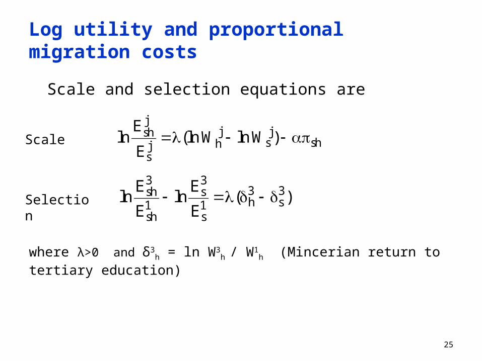
Log utility and proportional migration costs Scale and selection equations are

jj jsh

s shhjs

Eln (ln W ln W )

E

3 33 3sh sh s1 1

sh s

E Eln ln ( )

E E

Scale

Selection

where λ>0 and δ3h = ln W3

h / W1h (Mincerian return to tertiary education)

26

Theory: The Borjas View of Negative Selection

lnW

Ss*

US Wage

Mx Wage

27

Linear utility versus log utility (clustered standard errors in parentheses, other regressors not shown)

js

jh WW

)WW()WW( 1s

3s

1h

3h

js

jh WlnWln

)( 1s

3h

Linear utility Log utility

Wages Scale Selection   Wages Scale Selection

0.018 -0.435

(0.029) (0.087)

0.072 -1.307

(0.013) (0.186)

Observations 2786 1393 Observations 2786 1393

R-squared 0.44 0.47 R-squared 0.29 0.17

Clusters 15 15   Clusters 15 15

In theory, all wage coefficients should be positive

28

Log utility model predicts negative selection

ARM

AUS

AUT

AZE

BEL

BFA

BGD

BGR

BHS

BLR

BOL BRA

BWA

CAF

CANCHE

CHL

CHN

CMRCOL

CRI

CZEDEU

DNK

DOM

ECUEGY

ESPEST

ETH

FINFRAGBR

GEO

GHA

GINGMB

GRC

GTMGUY

HKG

HND

HRV

HUN

IDN

IRLISR

ITA

JAM

JOR

JPN

KAZ

KGZ

KOR

LSO

LTU

LUXLVA

MDA

MDG

MEX

MKD

MLI

MUS

MYS

NGA NIC

NLDNOR

NPL

NZLPAK

PAN

PERPHL

POL

PRT

PRY

ROM

RUS

SEN

SGP

SLV

SVKSVNSWE

SWZ

THA

TJK

TKM

TTO

TUR

UGA

UKR USA

UZB

VEN

VNM

ZAF

ZMB

ZWE

.51

1.5

22.

53

log

inco

me

80th

- 2

0th

pctil

es

-4 -2 0 2 4log income 20th pctile

neg. selection of mig. to US

neg. selection of mig. to Ger.

29

While linear utility model predicts negative selection

ARM

AUS

AUT

AZE

BEL

BFABGD

BGR

BHS

BLRBOL

BRABWA

CAF

CAN

CHE

CHL

CHNCMR

COLCRI

CZE

DEU

DNK

DOMECUEGY

ESP

EST

ETH

FIN

FRAGBR

GEOGHAGINGMB

GRC

GTMGUY

HKG

HND

HRVHUN

IDN

IRLISR

ITA

JAMJOR

JPN

KAZ

KGZ

KOR

LSO

LTU

LUX

LVA

MDAMDG

MEX

MKD

MLI

MUSMYS

NGA

NIC

NLD

NOR

NPL

NZL

PAK

PANPERPHL

POL

PRT

PRYROM

RUS

SEN

SGP

SLVSVK

SVN

SWE

SWZTHA

TJK

TKM

TTOTUR

UGA

UKR

USA

UZB

VEN

VNM

ZAF

ZMB

ZWE

05

1015

2025

inco

me

80th

- 20

th p

ctile

s, 0

00s

US

D

0 5 10 15 20income 20th pctile, 000s USD

pos. selection of mig. to US

pos. selection of mig. to Ger.

30

Data strongly support positive selection of emigrants

Afghanistan

AlbaniaAlgeria

Angola

Argentina

Armenia

Australia

Austria

Azerbaijan

Bahamas, The

BahrainBangladesh

Barbados

BelarusBelgium

Benin

Bhutan

Bolivia

Bosnia and Herzegovina

BotswanaBrazil

Brunei

Bulgaria

Burkina Faso

Burundi

CambodiaCameroon

Canada

Cape Verde

Central African Republic

Chad

ChileChina

Colombia

ComorosCongo, Dem. Rep.

Congo, Rep.

Costa RicaCote d'Ivoire

CroatiaCuba Cyprus

Czech RepublicDenmark

Djibouti

Dominican RepublicEast Timor

Ecuador

Egypt

El Salvador

Equatorial Guinea

Eritrea

EstoniaEthiopia

Fiji

Finland

France

Gabon

Gambia, The

Georgia

Germany

Ghana

Greece

Guatemala

Guinea

Guinea-Bissau

GuyanaHaiti

HondurasHong Kong

HungaryIceland

India

Indonesia

IranIraq

Ireland

IsraelItaly

Jamaica

Japan

Jordan

Kazakhstan

Kenya

KoreaKuwait

Kyrgyzstan

Lao PDR

Latvia

Lebanon

Lesotho

Liberia

Libya

LithuaniaLuxembourg

Macao, China

Macedonia

Madagascar

Malawi

MalaysiaMali

Malta

Mauritania

Mauritius

Mexico

Moldova

Mongolia

Morocco

Mozambique

MyanmarNamibiaNepal

Netherlands

New ZealandNicaragua

Niger

NigeriaNorway

Oman

PakistanPanama

Papua New Guinea

ParaguayPeru

PhilippinesPolandPortugal

Qatar

Romania

Russia

Rwanda

Saudi Arabia

SenegalSerbia

Sierra Leone

Singapore SlovakiaSlovenia

Solomon Islands

Somalia

South Africa

Spain

Sri Lanka

Sudan

Suriname

Swaziland

Sweden

SwitzerlandSyrian Arab Republic

Taiwan

Tajikistan

Tanzania

Thailand

Togo

Trinidad and Tobago

Tunisia

Turkey

Turkmenistan

UK

US

Uganda

Ukraine

United Arab Emirates

Uruguay

Uzbekistan

Venezuela, RB

Vietnam

West Bank and Gaza

ZambiaZimbabwe

-8-6

-4-2

02

Log

odds

of e

mig

ratio

n fo

r ter

tiary

edu

cate

d

-8 -6 -4 -2 0 2Log odds of emigration for primary educated

31

Why negative selection fails: productivity differences International wage differences

Suppose in Nigeria Tertiary educated earn $5,000 a year, while primary educated earn

$1,000 (meaning return to extra year of education is 20%)

while in the US Tertiary educated earn $40,000 a year, while primary educated earn

$20,000 (meaning return to extra year of education is 8%)

Predicted pattern of migrant selection Proportional-cost model predicts negative selection: δN – δUS > 0

Fixed-cost model predicts positive selection: WTUS- WT

N > WPUS- WP

N

Because of large differences in US-Nigerian raw labor productivity, gain to migration is higher for tertiary educated

32

Positive selection versus negative selection Condition for migrants to be positively selected by skill

Ignoring migration costs, condition becomes

13 31sh sh

1 3 1 3s s s h

gW 1W (W W )

31sh

1 3s h

WW

Ratio of return to skill in source relative to destination (>1)

Ratio of labor productivity in destination relative to source (>1)

33

Estimating fixed migration costs

Scale equation with source-destination fixed effects is an alternative way to write the selection equation

Estimate equation with a full set of source-destination dummies

Divide dummy coefficients by –α to estimate fixed costs fsh

To capture skill specific migration costs, include controls for costs (xsh) interacted with dummy for skill group

jj jjsh

s sh j shh shjs

Eln (W W ) f x

E

34

Estimated fixed migration costs, selected countries (000s of 2000 USD, relative to US-Mexico migration costs)

Destination

Source Australia Canada France Germany UK US

China 80.3 56.8 90.8 88.6 87.7 55.6Guatemala 105.8 45.0 83.8 80.1 96.9 8.9Jamaica 76.8 -1.7 67.2 51.0 -9.3 -3.0Mexico 117.0 59.6 90.5 82.5 90.6 0.0Poland 45.6 26.4 27.9 5.2 42.9 29.8

Turkey 63.2 68.0 40.1 7.9 53.3 60.4

Vietnam 39.6 31.0 38.5 45.5 61.8 21.0

35

(III) Sorting

36

Sorting equation

Collect terms with source country subscripts in selection equation (ie, add source fixed effects), which yields:

Only requires data on wages in destination

Common coefficient on wages in scale, selection, sorting eqs.

s1sh

3sh

1h

3h1

sh

3sh )gg()WW(

EEln

)WW()E/Eln( 1s

3s

1s

3ss

37

Estimating equations

Scale equation (assume fsh and gjsh are function of xsh)

Selection equation (assume gjsh is function of xsh)

Sorting equation (assume gjsh is function of xsh)

jj jj 3sh

s sh shh shjs

Eln (W W ) x I( j 3) x

E

'x)]WW()WW[(EEln

EEln j

shsh1s

3s

1h

3h1

s

3s

1sh

3sh

shssh1h

3h1

sh

3sh x)WW(

EEln

38

Earnings and Taxes

Earnings data from household surveys in rich countries Luxembourg Income Survey

Adjusting for tax treatment across OECD destinations

Low-wage tax rate (67% of average production worker wage)

High-wage tax rate (167% of average production worker wage)

Tax rate includes income taxes net of benefits (as tallied by OECD) plus both sides of the payroll tax

Rates are averaged over 1996-2000

39

LIS data on wage levels and differences (000s USD)Tax treatment Pre Pre Pre Post Post Post

Percentile 20th 80th Diff. 20th 80th Diff.

Australia 17.31 34.96 17.66 14.04 23.73 9.69

Austria 16.62 30.89 14.27 10.15 16.11 5.96

Canada 16.48 39.78 23.30 11.93 25.63 13.69

Denmark 27.68 54.49 26.81 16.26 26.06 9.80

France 13.62 30.36 16.74 7.86 14.50 6.64

Germany 24.84 48.08 23.24 13.29 21.32 8.03

Ireland 16.23 31.36 15.13 12.23 17.49 5.26

Netherlands 27.99 47.38 19.38 16.88 26.44 9.56

Norway 23.08 49.99 26.92 15.16 27.84 12.68

Spain 12.14 26.05 13.91 8.05 15.37 7.33

Sweden 18.81 37.75 18.93 9.75 16.92 7.17

US 24.30 64.67 40.37 17.22 40.98 23.76

UK 22.44 48.60 26.16 16.50 31.97 15.47

40

Regression results (other regressors suppressed)Table 4: Regression results from linear-utility model Equation: Scale Selection Sorting Sorting Sorting Sorting Wage data source: WDI/

WIDER WDI/

WIDER WDI/

WIDER WDI/

WIDER LIS LIS

Variable (1) (2) (3) (4) (5) (6) j

sj

h WW 0.018

(0.029) )WW()WW( 1

s3s

1h

3h 0.072

(0.013) )WW( 1

h3h , pre-tax 0.060 0.026

(0.026) (0.013) )WW( 1

h3h , post-tax 0.103 0.048

(0.045) (0.022) Observations 2786 1393 1393 1393 1214 1214 R-squared 0.44 0.47 0.61 0.61 0.63 0.63 Clusters 15 15 15 15 13 13

similarity of coefficients pre vs. post tax

41

Additional regressorsEquation: Selection Sorting Sorting Wage data source: WDI WDI LIS Variable (2) (4) (6) Anglophone dest. 0.567 0.636 0.678 (0.183) (0.256) (0.241) Common language 1.268 0.352 0.332 (0.248) (0.139) (0.124) Contiguous -0.384 -1.007 -1.097 (0.373) (0.237) (0.240) Longitude diff. -0.009 0.004 0.005 (0.003) (0.002) (0.003) Log distance 0.676 -0.259 -0.279 (0.131) (0.097) (0.111) LT colonial rel. -0.711 -0.445 -0.550 (0.193) (0.161) (0.137) ST colonial rel. -0.395 -0.187 -0.224 (0.431) (0.257) (0.276) Visa waiver -0.299 0.364 0.471 (0.135) (0.172) (0.203) Schengen sig. 0.402 0.403 0.507 (0.166) (0.252) (0.304) Asylee share -2.512 -3.635 -4.007 (0.818) (0.709) (0.810) Observations 1393 1393 1214 R-squared 0.47 0.61 0.63

42

Decomposing the immigrant skill gap

Why do some destinations get more skilled migrants?

Redefine key variables to write sorting regression as:

By properties of OLS, we have

Differencing between US, destination h yields immigrant skill gap decomposition

sh 0 1 sh 2 h s shy x W

h 0 1 h 2 h hˆ ˆ ˆ ˆy x W

US h 1 US h 2 US h US hˆ ˆ ˆ ˆy y x x W W

43

Skill gaps among destination countriesMean Skill Levels among Immigrants, by Destination Country

DestinationMean log skill share

Mean share

tertiary educated

Mean share

primary educated

Immigrant skills gap

USA 2.01 0.58 0.11 0.00Ireland 1.39 0.53 0.14 0.62Canada 1.30 0.68 0.22 0.71Australia 1.29 0.56 0.18 0.72Norway 1.15 0.37 0.13 0.86New Zealand 0.71 0.48 0.25 1.30United Kingdom 0.40 0.41 0.28 1.61Sweden 0.28 0.36 0.27 1.73Spain -0.03 0.25 0.25 2.04France -0.10 0.40 0.44 2.11Germany -0.31 0.37 0.49 2.32Denmark -0.51 0.27 0.42 2.52Austria -0.54 0.25 0.39 2.55Netherland -0.54 0.26 0.44 2.55Finland -0.75 0.26 0.51 2.76

44

Explaining the immigrant skill gap

Destination Wage diff. Share asylee Share explained ResidualAustralia 0.84 -0.07 0.78 0.22Austria 0.36 0.39 0.98 0.02Canada 0.99 -0.13 0.76 0.24Denmark 0.28 0.36 0.87 0.13Finland 0.38 0.09 0.68 0.32France 0.44 0.22 0.96 0.04Germany 0.44 0.05 0.76 0.24Ireland 1.52 0.83 1.95 -0.95Netherland 0.32 0.55 1.10 -0.10New Zealand 0.64 -0.26 0.32 0.68Norway 0.53 0.40 1.64 -0.64Spain 0.50 -0.06 0.74 0.26Sweden 0.55 0.36 1.27 -0.27UK 0.35 0.22 0.58 0.42

Mean 0.58 0.21 0.96 0.04

Share of immigrant skill gap explained by variables in sorting regression (other regressors not shown)

45

Concluding remarks Dominant features of international migration are small scale,

positive selection and positive sorting A simple model of income maximization can go a long way in

accounting for these outcomes

Wage differences contribute to positive selection and why educated migrants choose Anglophone countries over continental Europe

Methodological issues Bilateral migration costs (broadly defined) appear to be large

Not controlling for unobserved bilateral migration costs yields inconsistent estimates of how wages affect migration

Models with log utility and proportional costs fail to explain scale or skill composition of emigration

Seemingly crude measures of absolute skill-based wage differences perform surprisingly well

46

Extra slides

47

Results for proportional migration costs (Borjas)Table 5: Regression results from log-utility model Equation: Scale Selection Sorting Sorting Sorting Sorting Wage data source: WDI/

WIDER WDI/

WIDER WDI/

WIDER WDI/

WIDER LIS LIS

Variable (1) (2) (3) (4) (5) (6) j

sjh WlnWln -0.435

(0.087) )( 1

s3h -1.307

(0.186) 3h , pre-tax 3.929 5.338

(0.767) (0.886) 3h , post-tax 3.342 4.146

(0.761) (1.297) Observations 2786 1393 1393 1393 1214 1214 R-squared 0.29 0.17 0.40 0.38 0.43 0.38 Clusters 15 15 15 15 13 13

48

Robustness checks

Measure wages adjusting for PPP

Use Freeman Oosterndorp measure of wages

Drop destination countries one by one to test IIA

Control for university quality, lagged migrant stock

Redefine high skilled as secondary or tertiary educated